Circumstellar Medium Interaction in SN 2018lab, A Low-Luminosity II-P Supernova observed with TESS

Abstract

We present photometric and spectroscopic data of SN 2018lab, a low luminosity type IIP supernova (LLSN) with a V-band peak luminosity of $-15.1\pm 0.1$ mag. SN 2018lab was discovered by the Distance Less Than 40 Mpc (DLT40) SNe survey only 0.73 days post-explosion, as determined by observations from the Transiting Exoplanet Survey Satellite (TESS). TESS observations of SN 2018lab yield a densely sampled, fast-rising, early time light curve likely powered by circumstellar medium (CSM) interaction. The blue-shifted, broadened flash feature in the earliest spectra ($<$2 days) of SN 2018lab provide further evidence for ejecta-CSM interaction. The early emission features in the spectra of SN 2018lab are well described by models of a red supergiant progenitor with an extended envelope and close-in CSM. As one of the few LLSNe with observed flash features, SN 2018lab highlights the need for more early spectra to explain the diversity of flash feature morphology in type II SNe.

1 Introduction

Type IIP/IIL supernovae (SNe II) are the result of core-collapse in stars $>$8 M_⊙, and are defined by the appearance of hydrogen in their spectra (Filippenko, 1997; Smartt et al., 2009). SNe II have proven to be a continuous population smoothly spanning a significant photometric, $-19.0\lesssim M_{\mathrm{V}}\lesssim-13.0$ mag at peak, and spectroscopic diversity (Anderson et al., 2014; Sanders et al., 2015; Valenti et al., 2016; Gutiérrez et al., 2017). The extrema of the SNe II distribution have been the subject of intense study. SNe II with peak magnitudes $M_{V}\geq-15.5$ are referred to as Low Luminosity (LL) SNe (Pastorello et al., 2004). The plateau luminosities of SNe II correlate with their photospheric expansion velocities (Hamuy & Pinto, 2002; Pejcha & Prieto, 2015). In line with this relation, LLSNe have the lowest expansion speeds ($\sim 1300-2500$ km s^-1 at 50 days post-explosion, Pastorello et al., 2004; Spiro et al., 2014) of all SNe II. LLSNe also have smaller ejecta kinetic energies ($\sim 0.1-0.5\times 10^{51}$ ergs, Pumo et al., 2017) and lower nickel masses ($\leq 10^{-2}$ M_⊙, Turatto et al., 1998; Pastorello et al., 2004; Spiro et al., 2014) than typical SNe II (Pastorello et al., 2004).

The progenitors of LLSNe are unclear, despite their similarities to more luminous SNe II. The controversy surrounding the progenitors of LLSNe began with the discovery and subsequent progenitor modeling of SN 1997D (Turatto et al., 1998; Benetti et al., 2001). The characteristics of SN 1997D were well-explained by models of both the core collapse of a $>$20 M_⊙ star with a large amount of fallback (Turatto et al., 1998; Zampieri et al., 1998) and of a star near the mass limit for undergoing core-collapse (8-10 M_⊙, Chugai & Utrobin, 2000). In the time since, studies have supported both high (Zampieri et al., 2003, $>$20 M_⊙) and low-mass (Pignata, 2013; Pumo et al., 2017; Lisakov et al., 2017, 2018; Kozyreva et al., 2022, 8-10 M_⊙) red supergiant (RSG) progenitor models. Models with less massive (8-10 M_⊙) progenitors have become popular in recent years as archival pre-explosion Hubble Space Telescope (HST) images have placed upper limits on the progenitor masses of numerous LLSNe (Van Dyk et al., 2003, 2012; Maund & Smartt, 2005; Li et al., 2006; Smartt et al., 2009; Fraser et al., 2011; Maund et al., 2014).

Electron-capture (EC) SNe, the result of O-Ne-Mg core collapse in super-Asymptotic Giant Branch (AGB) stars, have also been used to explain the properties of some LLSNe (Hosseinzadeh et al., 2018; Valerin et al., 2022). Some models predict that ECSNe can appear nearly identical to low luminosity core collapse (CC) SNe (Nomoto, 1984; Kitaura et al., 2006; Poelarends et al., 2008) and their progenitors lie in the same mass range (super-AGB stars 8-10 M_⊙, Kitaura et al., 2006) as low mass RSGs which undergo core-collapse. Reliably distinguishing between the ECSNe and low luminosity CCSNe populations remains a challenge (Zhang et al., 2020; Hiramatsu et al., 2021a; Callis et al., 2021).

All massive stars are expected to lose mass, however the properties of mass loss (e.g. density, radial extent, physical location) vary for different progenitors (Smith, 2014). Therefore, the extent of ejecta-CSM interaction is a possible indicator of whether an LLSN is from an electon-capture or core-collapse. Super-AGB stars readily produce large CSM envelopes as a result of their thermal pulsation phase. RSGs often have nearby CSM as well, though often much less than super-AGB stars, due to late stage episodic and eruptive mass loss. Indicators of ejecta-CSM interaction are sometimes only visible in the hours and days immediately following a SN explosion, before the SN ejecta has completely overtaken any CSM. Ejecta-CSM interaction can result in increased luminosity within the first weeks following explosion, observed as a bump or fast rise in the early light curve (Anderson et al., 2014; González-Gaitán et al., 2015; Valenti et al., 2016; Morozova et al., 2017, 2018; Förster et al., 2018; Hiramatsu et al., 2021b). More dense and substantial CSM will result in a larger – and possibly longer – excess luminosity and a greater effect on the early light curve. LLSNe with pronounced early time light curve bumps, like SN 2016bkv (Hosseinzadeh et al., 2018), may have super-AGB progenitors.

Narrow emission lines observed in the spectra of SNe in the days following explosion can be used to indicate the composition, density, and velocity of the CSM surrounding the progenitor (Gal-Yam et al., 2014). These narrow lines, often referred to as “flash” spectroscopy, are the result of recombination of CSM ionized by the shock-breakout flash (Khazov et al., 2016) or very early ejecta-CSM interaction (Smith et al., 2015; Shivvers et al., 2015) which ends when the CSM is entirely swept up by the expanding ejecta.

Narrow lines from ionized CSM have been detected in the hours following explosion in some instances (Niemela et al., 1985; Benetti et al., 1994; Quimby et al., 2007; Gal-Yam et al., 2014). When these spectral features are detected, they can provide insight into the composition and mass-loss history of the progenitor (Groh et al., 2014; Yaron et al., 2017; Davies & Dessart, 2019). To date the only LLSN that clearly exhibits narrow early time flash features is SN 2016bkv (Hosseinzadeh et al., 2018).

A few SNe have shown signs of broadened, blue-shifted features rather than narrow ones in the days following explosion (Soumagnac et al., 2020; Bruch et al., 2021; Hosseinzadeh et al., 2022). These broad features, hereafter referred to as broad-lined flash features, are produced when the outer layers of SN ejecta interact with low density CSM. The substantial CSM surrounding a super-AGB progenitor is likely to produce narrow lines at $\sim$5 days which can persist for up to a week, whereas CSM surrounding a RSG progenitor produces flash features which are typically expected to broaden and fade by $\sim$5 days post-explosion (Hiramatsu et al., 2021a). We must emphasize that the prolonged existence of narrow-lined flash features in and of itself does not distinguish super-AGB progenitors from RSG progenitors. Some SNe with RSG progenitors exhibit narrow-lined flash features that remain visible for over a week (SN 1998S, Leonard et al. 2000, Fassia et al. 2001; SN 2020tlf, Jacobson-Galán et al. 2022) and while the suggested ECSN SN 2018zd has long-lived narrow-lined flash features (Hiramatsu et al., 2021a), SN 2018zd might be a CCSN with a RSG progenitor (Zhang et al., 2020; Callis et al., 2021). However, no LLSN with narrow-lined flash features has a confirmed RSG progenitor. So in LLSNe, short-lived, early-time, broadened, blue-shifted flash features could be an indicator of a RSG progenitor rather than a super-AGB one, assuming there is no extreme long-term mass loss around the RSG.

In this work, we present spectroscopic and photometric data for SN 2018lab, a LLSN which displays clear signs of CSM interaction: a fast rising light curve and a broad-lined flash feature in the early spectra ($<$2 days). In Section 2 the discovery and classification of SN 2018lab is reviewed. In Section 3 the observations and data reduction are outlined. In Section 4 the photometric evolution is discussed. In Section 5 we present the spectroscopic evolution. These results are summarized in Section 6.

2 Discovery and Classification

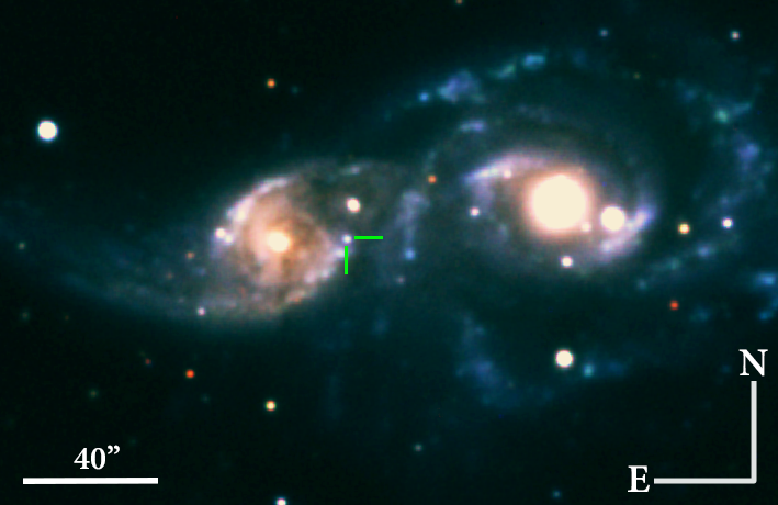
Figure 1: Composite $g,r,i$ image of SN 2018lab (indicated by green tick marks) in IC 2163 (left) obtained by Las Cumbres Observatory on 2019 January 10. NGC 2207 is on the right.

SN 2018lab, also known as DLT18ar, was first discovered, at RA(2000) = $06\overset{\mathrm{h}}{\phantom{.}}16\overset{\mathrm{m}}{\phantom{.}}26\overset{\mathrm{s}}{.}520$ and Dec(2000) = $-21\overset{\circ}{\phantom{.}}22\overset{\prime}{\phantom{.}}32\overset{\prime\prime}{.}38$, by the Distance Less Than 40 Mpc Survey (DLT40, for survey details see Tartaglia et al., 2018) on 2018-12-29 at 03:01:26 UTC (58481.126 MJD; Sand et al., 2018).

The redshift of SN 2018lab is $z_{\mathrm{18lab}}=0.0089$, measured using the host H$\alpha$ in the first spectrum (1.6 days after explosion). SN 2018lab is located between the interacting galaxies IC 2163 and NGC 2207 (see Figure 1). IC 2163 and NGC 2207 are a well-studied pair of interacting, grazing galaxies (Elmegreen et al., 1995b, a, 2001, 2006; Struck et al., 2005) that frequently produce SNe, notably SN 1975A (Kirshner et al., 1976; Arnett, 1982), SN 2003H (Filippenko et al., 2003; Lyman et al., 2014), SN 2010jp (Smith et al., 2012; Corgan et al., 2022), SN 2013ai (Davis et al., 2021), and SPIRITS 14buu, 15c and 17lb (Jencson et al., 2017, 2019). IC 2163 has a redshift $z=0.0090$ (de Vaucouleurs et al., 1991) and NGC 2207 has a redshift $z=0.0092$ (Springob et al., 2005). The measured redshift to SN 2018lab is most consistent with that of IC 2163, which is quoted as the host galaxy throughout this work.

IC 2163 was in the Transiting Exoplanet Survey Satellite (TESS; Ricker et al., 2015) footprint when SN 2018lab exploded. TESS observations of SN 2018lab yield an explosion date of MJD 58480.4$\pm$0.1, as published in Vallely et al. (2021, see their Eq. 2 and Table 1). This explosion time is 0.24 days after the last DLT40 non-detection and 0.73 days before DLT40’s discovery of SN 2018lab, as seen in Figure 2. We adopt the TESS-derived explosion epoch throughout this work. Spectroscopic classification done on 2018-12-31 at 06:42:29 UTC, 2 days after the explosion, confirmed that the object was an SN II (Razza et al., 2018).

3 Observations and Data Reduction

3.1 Follow-up Photometry and Spectroscopy

3.1.1 Photometry

SN 2018lab was observed by TESS during the mission’s Sector 6 operations, from 2018-12-15 18:36:03.542 to 2019-01-06 12:36:19.181 UTC. The TESS lightcurve of SN 2018lab was previously published in Vallely et al. (2021). In Figure 2, the TESS photometry, both unbinned and rolling 6-hr medians, is plotted.

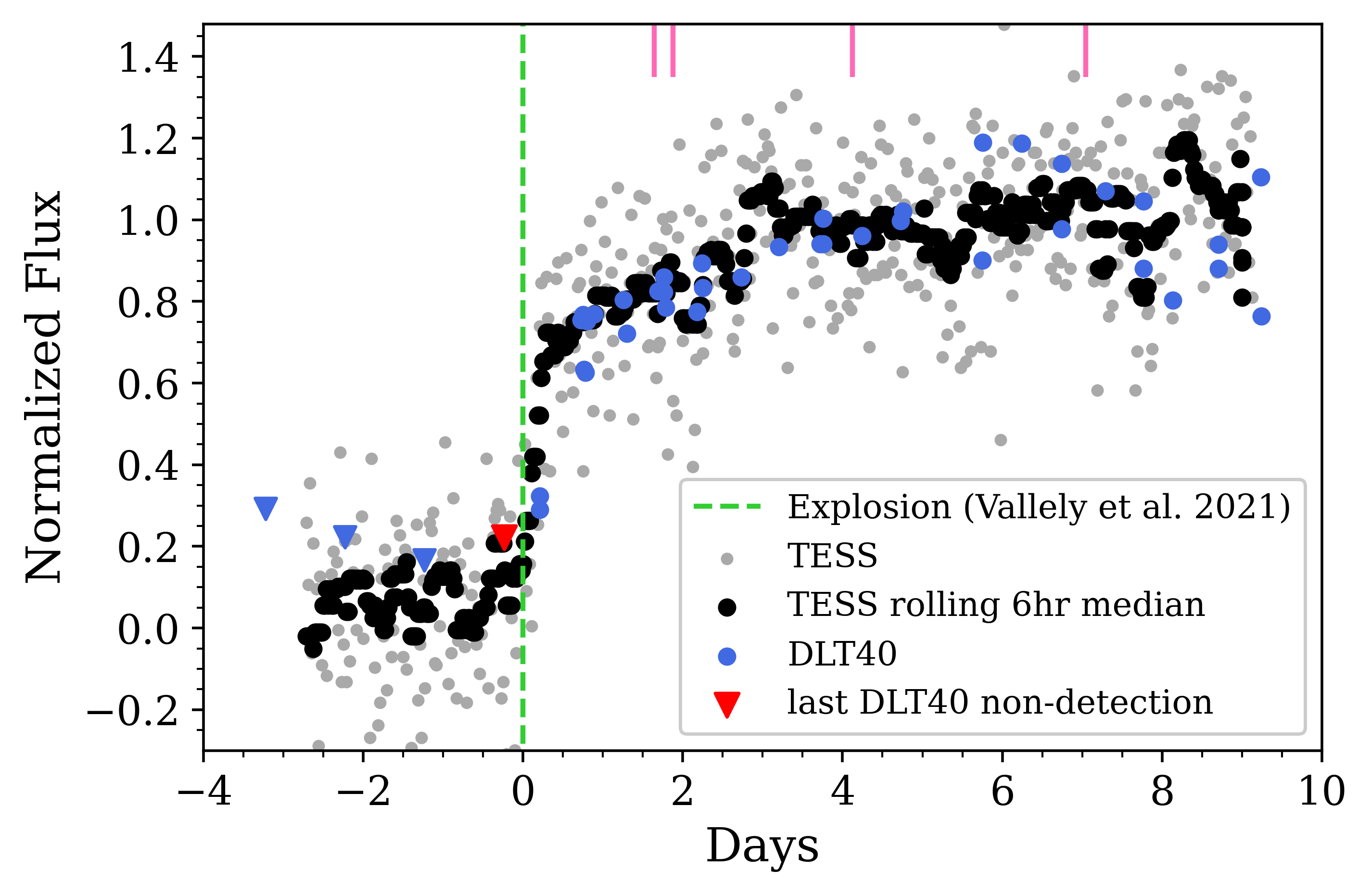
Figure 2: TESS-band SN 2018lab light curve (gray and black) and r-band corrected DLT40 (blue and red) data. Times of spectral epochs are marked in pink ticks at the top. The explosion time as reported in Vallely et al. (2021) is marked by the green dashed line. This value is extremely well constrained by both TESS and DLT40 observations (see Figure 3 for zoomed in version). The light curves are normalized to the median value of the data 3–8 days after explosion.

Following the discovery of SN 2018lab by the DLT40 survey, continued monitoring was done by two of DLT40’s discovery telescopes, the PROMPT5 0.4m telescope at the Cerro Tololo Inter-American Observatory and the PROMPT-MO 0.4m telescope at the Meckering Observatory in Australia. Observations taken by these telescopes are calibrated to the SDSS r band, as described in Tartaglia et al. (2018), and are shown in Figure 2.

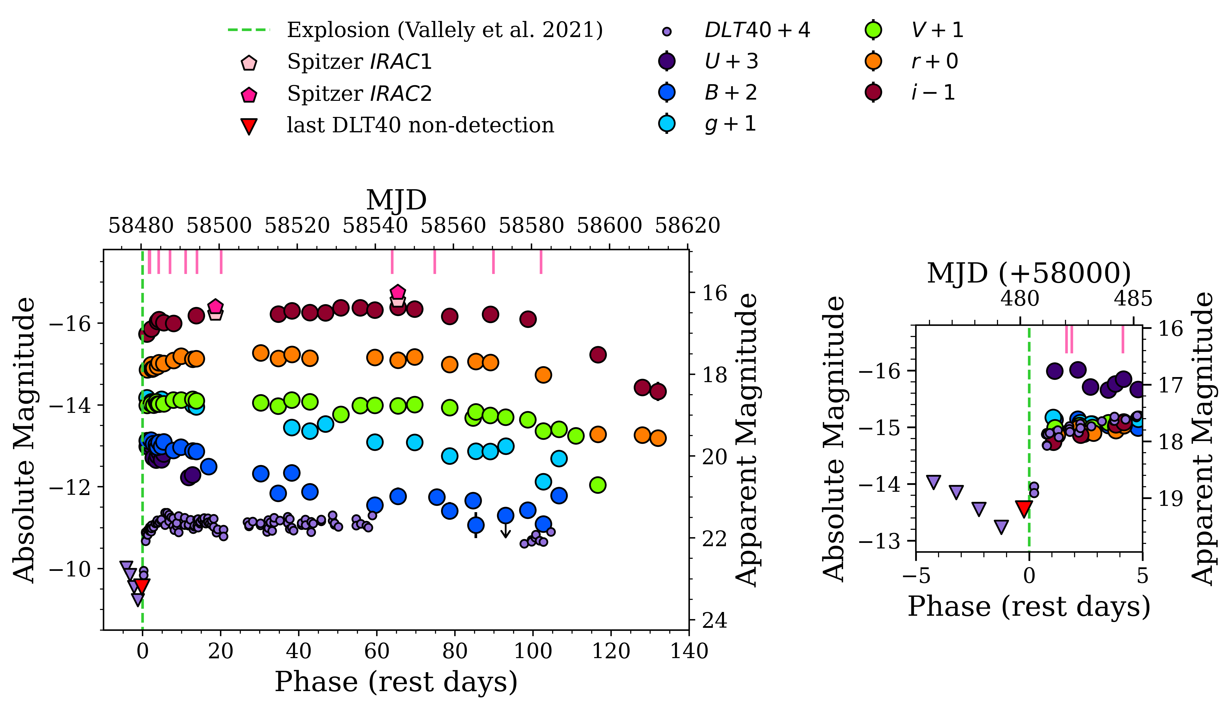
Figure 3: SN 2018lab light curves from DLT40, Las Cumbres Observatory, and Spitzer/IRAC. Left: light curves with offsets. Right: zoom in of the light curve in the first 5 days after explosion without offsets. Spectroscopic epochs are shown as pink lines along the upper x-axis.

Additional UBVgri photometry of SN 2018lab was obtained using the Sinistro cameras on Las Cumbres Observatory’s robotic 1m telescopes (Brown et al., 2013), located at the Siding Spring Observatory, the South African Astronomical Observatory, and the Cerro Tololo Inter-American Observatory. These are shown in Figure 3

The photometric data from Las Cumbres Observatory was reduced using lcogtsnpipe (Valenti et al., 2016), a PyRAF-based image reduction pipeline. Given the complexity of the host, UBVgri reference images were obtained with Las Cumbres Observatory on 2021 August 25, $>$900 days after explosion, when the SN was no longer bright enough to be detectable. These reference frames were subtracted from the science images. Aperture photometry was then extracted from the difference images using lcogtsnpipe. Apparent magnitudes were calibrated to the APASS (BVgri) catalog and Landolt (U) standard fields observed on the same nights with the same telescopes.

Infrared photometry of SN 2018lab was also obtained with images from the Infrared Array Camera (IRAC, Fazio et al., 2004) on board the Spitzer Space Telescope (Werner et al., 2004; Gehrz et al., 2007). The host system was imaged several times between 2014–2019 in the IRAC1 ($3.6$ $\mu$m) and IRAC2 ($4.5$ $\mu$m) imaging bands by the SPitzer InfraRed Intensive Transients Survey (SPIRITS; PI M. Kasliwal; PIDs 10136, 11063, 13053, 14089). The “postbasic calibrated data”-level images were downloaded from the Spitzer Heritage Archive and processed through an automated image subtraction pipeline (for survey and pipeline details, see Kasliwal et al., 2017; Jencson et al., 2019). For reference images, we used the Super Mosaics, consisting of stacks of images obtained on 2005 February 2. Aperture photometry was performed on the difference images adopting the appropriate aperture corrections and Vega-system zeropoint fluxes from the IRAC instrument handbook and following the method for a robust estimate of the photometric uncertainties as described in Jencson (2020). These data are presented in Figure 3.

3.1.2 Spectroscopy

We present 12 optical spectra of SN 2018lab ranging from less than 48 hours to over 300 days after explosion. Of the 12 spectra presented in this work, 11 were obtained as a result of a high-cadence spectroscopic follow up campaign using the Robert Stobie Spectrograph (RSS) on the Southern African Large Telescope (SALT, Smith et al., 2006) using a 1.50” slit width, the FLOYDS instruments (Brown et al., 2013) on the Las Cumbres Observatory’s 2m Faulkes Telescopes North and South (FTN/FTS) with the set up described in Brown et al. (2013) with a 2” slit width, the Low Resolution Imaging Spectrometer (LRIS, Oke et al., 1995) on Keck I using a 1.5” slit width, and one of the Multi-Object Double Spectrographs (MODS1, Pogge et al., 2010) on LBT in the 1.0” segmented longslit configuration. The LBT spectrum from 308 days post-explosion is discussed in Section 5.4. We also include in our analysis the classification spectrum from 1.9 days post-explosion (Razza et al., 2018) taken as part of the Public European Southern Observatory (ESO) Spectroscopic Survey for Transient Objects (ePESSTO, Smartt et al., 2015) using the ESO Faint Object Spectrograph and Camera (EF0SC2) on the ESO New Technology Telescope (ESO-NTT) using a 1” slit width with the Grism#13 described in Smartt et al. (2015). All spectra are logged in Table 1.

Date	JD	Epoch (day)	Telescope	Instrument	Exposure (s)
2018-12-30	2458482.5411	1.6	SALT	RSS	1994.0
2018-12-30	2458482.7795	1.9	ESO-NTT	EFOSC2	600.0
2019-01-01	2458485.0255	4.1	FTS 2m	FLOYDS	3600.0
2019-01-04	2458487.9443	7.0	FTN 2m	FLOYDS	3600.0
2019-01-08	2458491.9115	11.0	FTN 2m	FLOYDS	3600.0
2019-01-11	2458494.8412	13.9	Keck I	LRIS+LRISBLUE	600.0
2019-01-17	2458500.9915	20.1	FTS 2m	FLOYDS	3600.0
2019-03-02	2458544.8102	63.9	FTN 2m	FLOYDS	3600.0
2019-03-13	2458555.7320	74.8	FTN 2m	FLOYDS	3600.0
2019-03-28	2458570.7291	89.8	FTN 2m	FLOYDS	3600.0
2019-04-09	2458582.9357	102.0	FTS 2m	FLOYDS	3600.0
2019-11-01	2458788.9488	308.0	LBT-SX	MODS1R	600.0

Table 1: Log of Spectroscopic Observations

3.2 Distance

We assume a distance modulus of 32.75$\pm{0.4}$ mag, based on the distance of 35.5 Mpc to IC2163/NGC2207 (Theureau et al., 2007). This distance is a mean of the JHK Tully-Fisher distances and was used in Jencson et al. (2017). This is consistent with the widely used distance to IC2163/NGC2207 of 35$\pm{2.5}$ Mpc (Elmegreen et al., 2017; Kaufman et al., 2016) and the measured distance to NGC 2207, using SN Ia 1975A, of 39.6$\pm{5.5}$ Mpc (Arnett, 1982). A recent paper on SN 2010jp (Corgan et al., 2022), which is in the vicinity of IC2163/NGC2207, uses a distance of 24.5 Mpc. However, Corgan et al. (2022) also suggests that the host galaxy of SN 2010jp is a foreground dwarf galaxy, not IC 2163 or NGC 2207, which accounts for the difference in distances.

Figure 4: Extinction corrected $B-V$ color for SN 2018lab compared with other SNe with similar light curve properties. The adopted $E(B-V)_{tot}=0.22$ is consistent with the color evolution of these similar SNe. Data shown for SN 2009ib (Takáts et al., 2015), SN 2009N (Takáts et al., 2014), SN 2005cs (Brown et al., 2007; Tsvetkov et al., 2006; Pastorello et al., 2009; Faran et al., 2014), SN 2003bl (Galbany et al., 2016), SN 2003E (Galbany et al., 2016), SN 2003bl (Anderson et al., 2014), and SN 2003E (Anderson et al., 2014).

3.3 Extinction

The equivalent widths of Na ID absorption lines correlate with interstellar dust extinction (Richmond et al., 1994; Munari & Zwitter, 1997). To estimate the extinction along the line of sight, the Na ID features in the Keck LRIS spectrum, which has a high signal-to-noise and resolving power $R=715$, were analyzed. The equivalent widths of both the $z=0$ (Milky Way) and the $z=0.0089$ (host) features were measured by fitting and integrating Gaussian line profiles. The equivalent widths were then converted to $E(B-V)$ using Eq 9. of Poznanski et al. (2012) with an additional normalization factor of 0.86 from Schlafly et al. (2010). This method gives a Milky Way extinction, $E(B-V)_{\mathrm{MW}}=0.058_{-0.0095}^{+0.012}$ mag, which is roughly consistent with the value from Schlafly & Finkbeiner (2011) of $0.0748\pm{0.0006}$ mag. We adopt the latter value. The equivalent width of the host Na ID doublet was close to 2 Å. The relation between the Na ID equivalent width and dust extinction given in Poznanski et al. (2012) saturates at an equivalent width of $\sim$0.2Å, so alternative methods of measuring SN 2018lab’s host extinction are required.

The diffuse interstellar band (DIB) absorption feature used in Phillips et al. (2013) can also be used to determine extinction, however the DIB was not visible in any of the SN 2018lab spectra. This was also the case for the KI $\lambda$7699 line, which is effective at determining the host extinction as well (Munari & Zwitter, 1997).

Host extinction is instead determined by comparing the color evolution of SN 2018lab to other SNe IIP with similar peak magnitudes and light curve shapes (light curve properties are described in Section 4), namely SN 2009ib (Takáts et al., 2015), SN 2009N (Takáts et al., 2014), SN 2003bl (Galbany et al., 2016; Anderson et al., 2014), and SN 2003E (Galbany et al., 2016; Anderson et al., 2014). This analysis gives a $E(B-V)_{\mathrm{host}}$ of about 0.15 (see Figure 4). Using this value, the dereddened spectra of 2018lab matches the continuum slope of other extinction corrected LLSNe. Given the location of SN 2018lab in a dusty spiral arm of a star forming galaxy, this level of local host galaxy reddening is not surprising. There is likely significant uncertainty in this value, however the scatter in $B$$-$$V$ color makes it difficult to make a better estimation of the host extinction (Figure 4). We note that SN 2018lab exhibits evidence of CSM interaction, which can make a SN appear slightly more blue and may cause the extinction to be underestimated using this method. The combined Milky Way and host extinction gives a $E(B-V)_{\mathrm{tot}}=0.22$ mag, which we adopt as the total extinction to the supernova.

4 Photometric Evolution

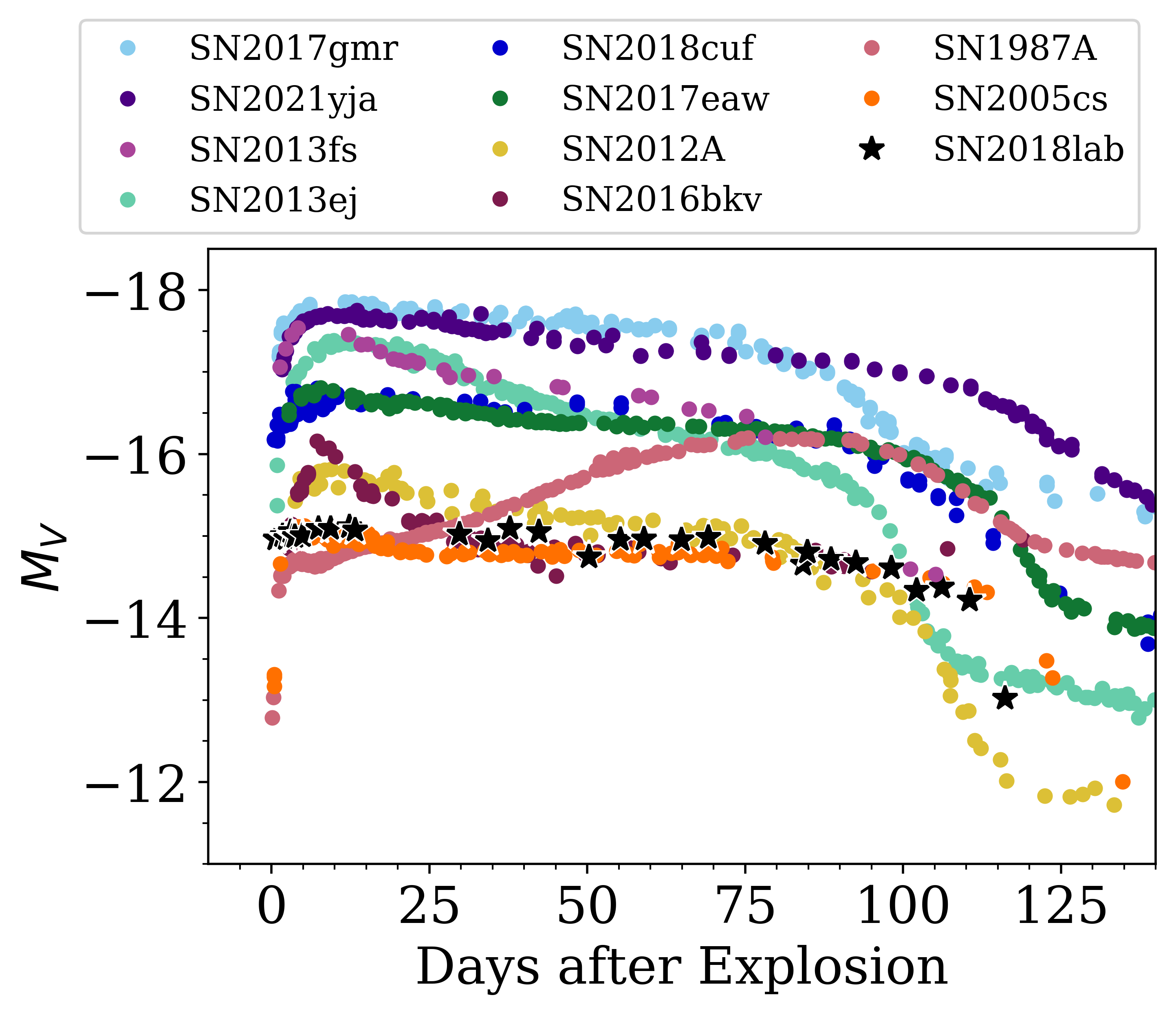
Figure 5: Absolute V-band light curve of SN 2018lab compared with other SNe II: SN 2017gmr (Andrews et al., 2019), SN 2021yja (Hosseinzadeh et al., 2022), SN 2013fs (Rubin et al., 2016; Valenti et al., 2016; Bullivant et al., 2018), SN 2013ej (Yuan et al., 2016; Huang et al., 2015; de Jaeger et al., 2019), SN 2018cuf (Dong et al., 2021), SN 2017eaw (Tsvetkov et al., 2018; Szalai et al., 2019), SN 2012A (Tomasella et al., 2013; de Jaeger et al., 2019), SN 2016bkv (Hosseinzadeh et al., 2018; Nakaoka et al., 2018), SN 1987A (Menzies et al., 1987; Catchpole et al., 1987; Suntzeff et al., 1988; Catchpole et al., 1988), and SN 2005cs (Brown et al., 2007; Tsvetkov et al., 2006; Pastorello et al., 2009; Faran et al., 2014). SN 2018lab has a peak V-band magnitude of $-$15.1 mag which is consistent with the luminosity of SN 2005cs, a notable LLSN.

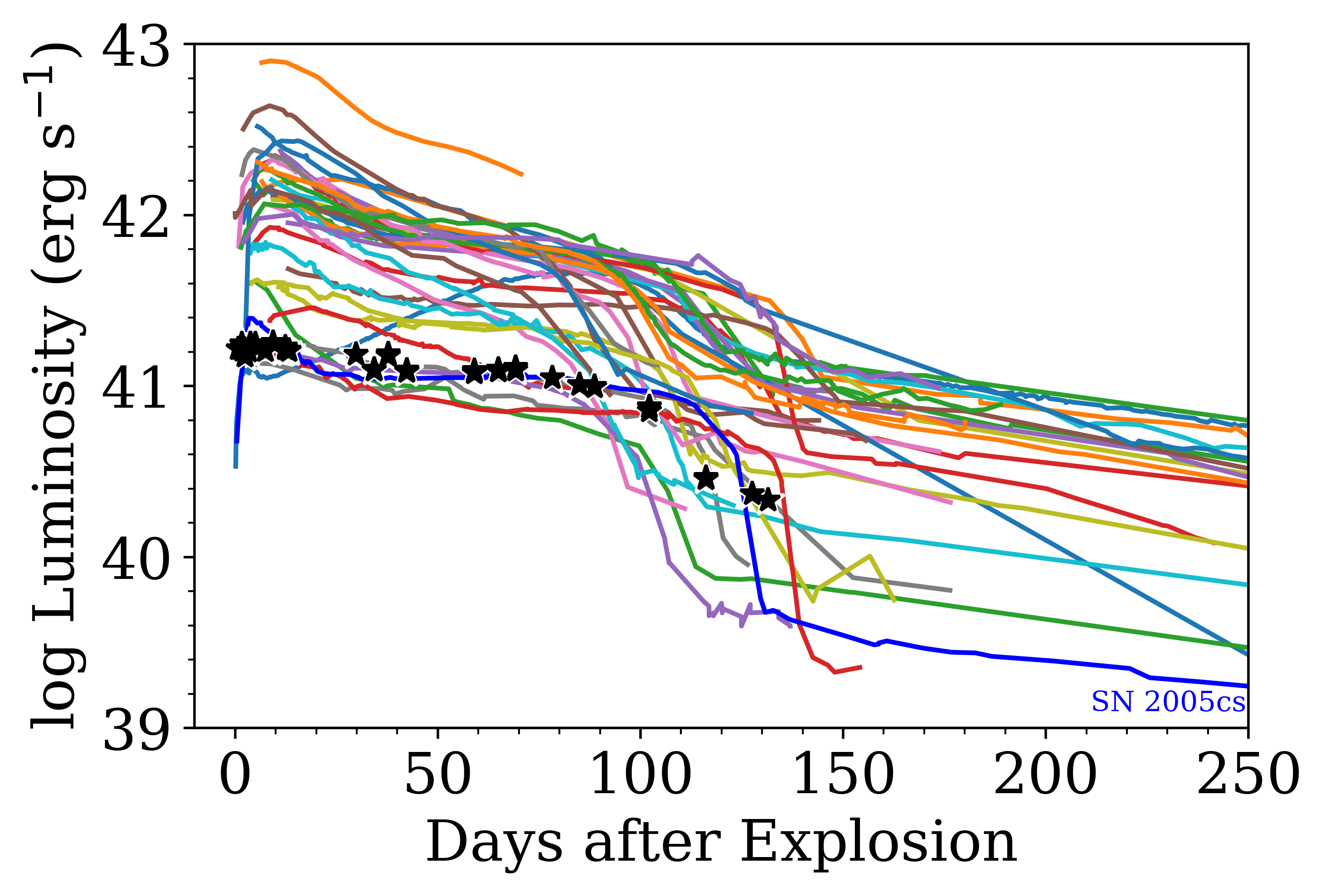
Figure 6: Bolometric light curve of SN 2018lab compared with other SNe II presented in Valenti et al. (2016). SN 2018lab has a peak luminosity of 10^41.2±0.1 erg s^-1. While SN 2018lab has a flatter and shorter plateau than SN 2005cs (blue), these features are not atypical for a LLSN.

In the V-band, SN 2018lab peaks at $-15.1\pm 0.1$ mag, consistent with the observed brightness of the archetype LLSN SN 2005cs (see Figure 5). Compared to SN 2005cs, the bolometric light curve of SN 2018lab remains fairly flat at the start of the plateau phase and has a shorter plateau duration. However, given a SN 2018lab peak luminosity of 10^41.2±0.1 erg s^-1, it fits well into the LLSN subclass, as shown in Figure 6.

The V-band decline rate of SN 2018lab in the 50 days following maximum brightness, denoted $s_{50}$, was measured according to the protocol outlined in Valenti et al. (2016). SN 2018lab has an extremely flat plateau phase, with a $s_{50}=0.13\pm 0.05$ mag/50 days. There are very few light curve points at the end of the plateau making it difficult to fit the transition to the nickel tail, and therefore we are unable to estimate a reliable ⁵⁶Ni mass. The last few points of the r band light curve have a slope of $<0.01$ mag/day, indicating that they may lie on the nickel tail. In order to get a rough estimate of the plateau length, we use the average time between the last point on the V band plateau and the first point on the tail in the r band to determine the plateau length $t_{PT}=113\pm 3$ days.

Vallely et al. (2021) models the light curves of 20 CCSNe observed by TESS including SN 2018lab (denoted as DLT18ar in their work) using a curved power-law (see their Eqn. 2). This method effectively reproduces the shape of SN 2018lab’s early light curve, and they find a rise time of $t_{\mathrm{rise}}=8.3\pm 0.21$ days, which is among the fastest in their sample of 20 SNe. Additionally, SN 2018lab was the lowest luminosity SN in the sample by almost 2 magnitudes, with a peak luminosity of $-15.48\pm 0.29$ mag in the TESS band.

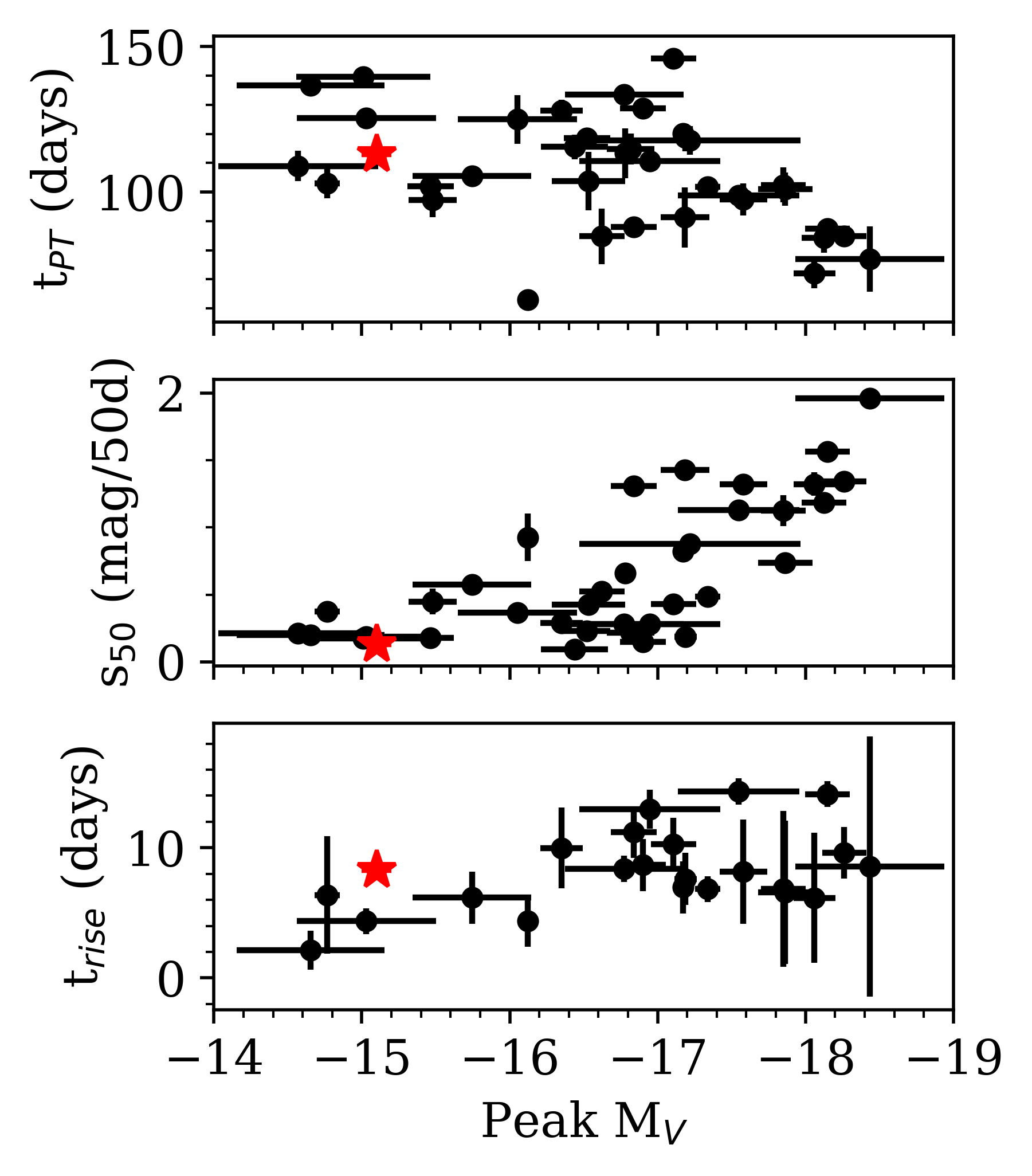
Figure 7: Comparison of the light curve properties of SN 2018lab to SNe in Valenti et al. (2016). Top: SN 2018lab has a plateau length, $t_{PT}$, in agreement with other SNe II. Middle: In the 50 days following peak magnitude, the slope of SN 2018lab’s light curve remains very flat, as is common in LLSNe. Bottom: Similar to other LLSNe, SN 2018lab rises to peak light quickly. Error bars on the SN 2018lab measurements are smaller than the marker.

The light curve properties of SN 2018lab (see Table 2) are in line with other LLSNe (see Figure 7). The peak V-band luminosities of LLSNe, including SN 2018lab, are less than a typical CCSNe by a factor of 10 (Pastorello et al., 2004). The typical plateau time of SNe II, including LLSNe, is 80-140 days (Valenti et al., 2016), in agreement with SN 2018lab’s $t_{PT}$. The peak luminosity and the decline rate of SNe II are related to one other, with LLSNe having much flatter plateaus (i.e. lower $s_{50}$ values) than more luminous SNe II (Anderson et al., 2014). The $s_{50}$ values for SNe II are $\lesssim$3 mag/50 days. Like other LLSNe, the $s_{50}$ of SN 2018lab lies on the low end of the $s_{50}$ continuum for SNe II. The rise times of SNe II are fast ($<$20 days) compared to other types of SNe; the rise times of LLSNe are on the faster end of the SNe II distribution with $t_{rise}\lesssim 10$ days (Valenti et al., 2016). The values of $s_{50}$, $t_{PT}$, and $t_{rise}$ for SN 2018lab are similar to other LLSNe in Valenti et al. (2016).

Table 2: SN 2018lab Parameters

Last Non-Detection	JD 2458480.6624
Discovery	JD 2458481.626
Explosion Epoch	JD 2458480.9 $\pm$ 0.1
Redshift $z$	0.0089 $\pm$ 0.0001
Distance (modulus $\mu$)	35.5 Mpc (32.75 mag)
$E(B-V)_{\mathrm{tot}}$	0.22 mag
$M_{\mathrm{TESS}}$ at peak4	$-15.48$ $\pm$ 0.29 mag
$t_{rise}$4	8.3 $\pm$ 0.21 days
$s_{50}$	0.13 $\pm$ 0.05 mag/50 days
$t_{PT}$	113 $\pm$ 3 days

4.1 Shock Cooling Model

The rising light curves of SNe II are in part powered by shock cooling—energy added to the stellar envelope by the core-collapse shock wave. To determine the effect of shock cooling on the rising light curve of SN 2018lab, the light curve is fit using the Light Curve Fitting package (Hosseinzadeh & Gomez, 2020) which employs the analytic method for modeling early SNe II light curves powered by shock cooling described in Sapir & Waxman (2017).

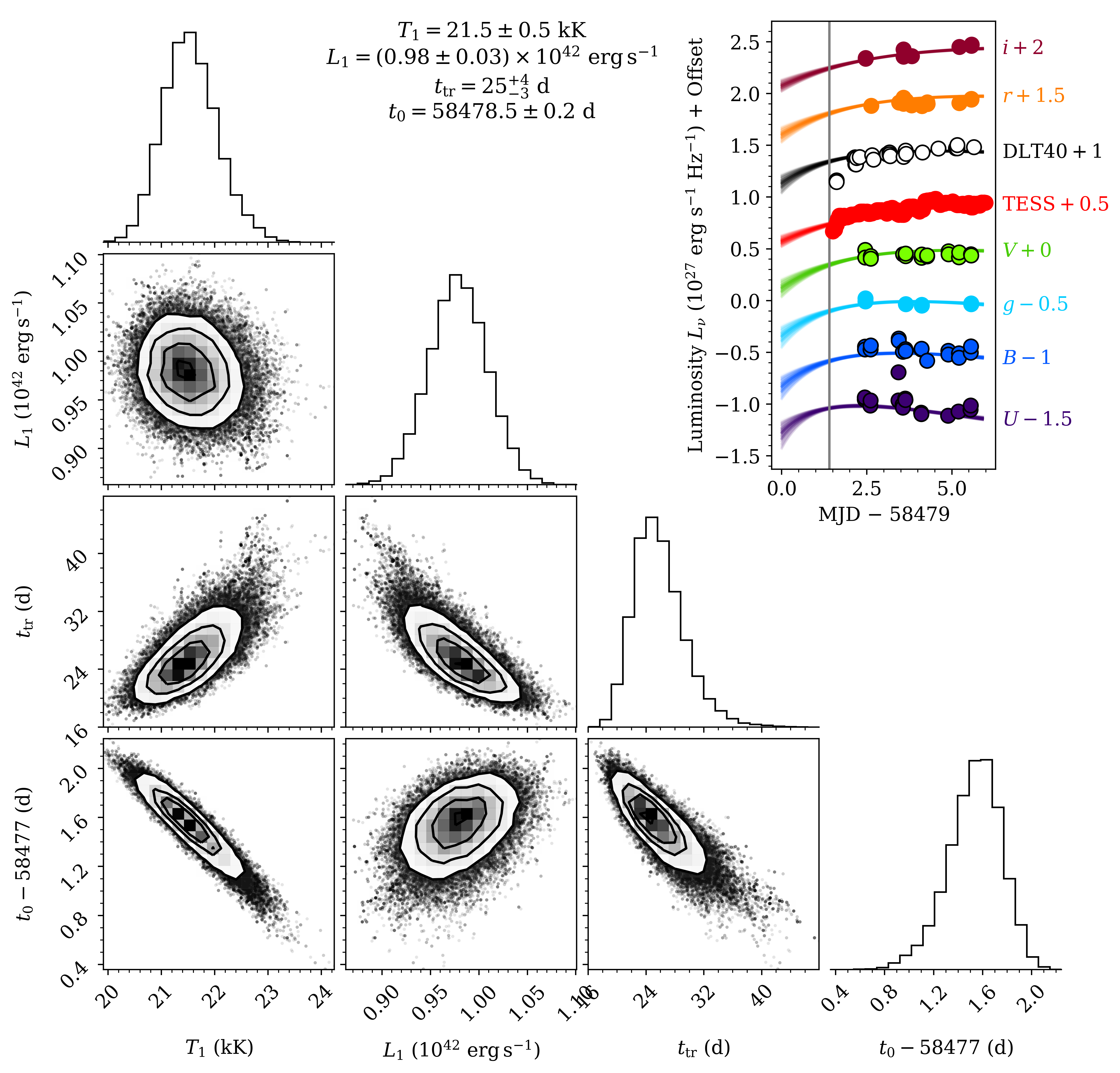
Figure 8: Posterior distributions of and correlations between the temperature 1 day after explosion ($T_{1}$), the total luminosity $\sim$1 day after explosion ($L_{1}$), the time at which the envelope becomes transparent ($t_{tr}$), and the explosion time ($t_{0}$). The 1$\sigma$ credible intervals, centered about the median, are given at the top. The top right panel shows 100 randomly drawn fits from the MCMC compared to the multiband light curve. The fit predicts an explosion time significantly ($>1$ day) before the explosion epoch (vertical grey line) constrained by TESS observations (Vallely et al., 2021) and DLT40 non-detections. The fit fails to describe SN 2018lab’s fast rising light curve (see the TESS and DLT40 light curves). This may indicate the presence of ejecta-CSM interaction, which is not accounted for in this model.

Degeneracies between the Sapir & Waxman model parameters makes it difficult to fit them independently in the case of SN 2018lab. Therefore, we use the version of the Sapir & Waxman model used in Hosseinzadeh et al. (2018) which utilizes scaling parameters: the temperature 1 day after explosion ($T_{1}$), the total luminosity $\sim$1 day after explosion ($L_{1}$), the time at which the envelope becomes transparent ($t_{tr}$), and the explosion time ($t_{0}$). This version of the model, with a polytropic index n=1.5 for a RSG progenitor density profile, was fit to the multiband light curve of SN 2018lab up to MJD 58485 (4.6 days after explosion). This was done with a Markov Chain Monte Carlo (MCMC) routine and flat priors for all parameters. The model gives the total luminosity and blackbody temperature as a function of time for each set of parameters. This is then converted to observed fluxes for each photometry point. Figure 8 shows the results of the MCMC, including the light curve fits, posterior distributions, and the 1$\sigma$ credible intervals centered on the medians.

The best fit models have difficulty reproducing the fast rise, completely missing the DLT40 and TESS rise points. The best fit explosion time is MJD 58478.5$\pm 0.2$, $>$1 day before the highly constrained explosion time estimated from the TESS data (MJD 58480.4$\pm$0.1, Vallely et al., 2021) and before two DLT40 non-detections. Further, the model fails to fit the rising light curve when the explosion time is fixed to be within the error of the TESS explosion epoch. Due to the failure of the model to accurately fit the steep rise in the light curve, we do not consider these models to be a good fit, but they are included here for completeness.

The failure of the shock cooling model to accurately predict the steep rise may be evidence of ejecta-CSM interaction, which is not accounted for in the Sapir & Waxman model. A steep rise can occur when the CSM is optically thick enough that shock breakout does not occur on the edge of the stellar envelope but rather outside of it, within the CSM. The gradual density gradient of the CSM means this shock breakout occurs at a lower density than for a bare RSG, allowing the shocked material to cool and expand faster, resulting in early excess flux, and therefore a steeper rise than would be expected for a SN without CSM (Morozova et al., 2017; Tinyanont et al., 2022). This explanation is bolstered by the presence of broad-lined flash features in the early spectra ($<2$ days post-explosion), to be discussed in Section 5.1.

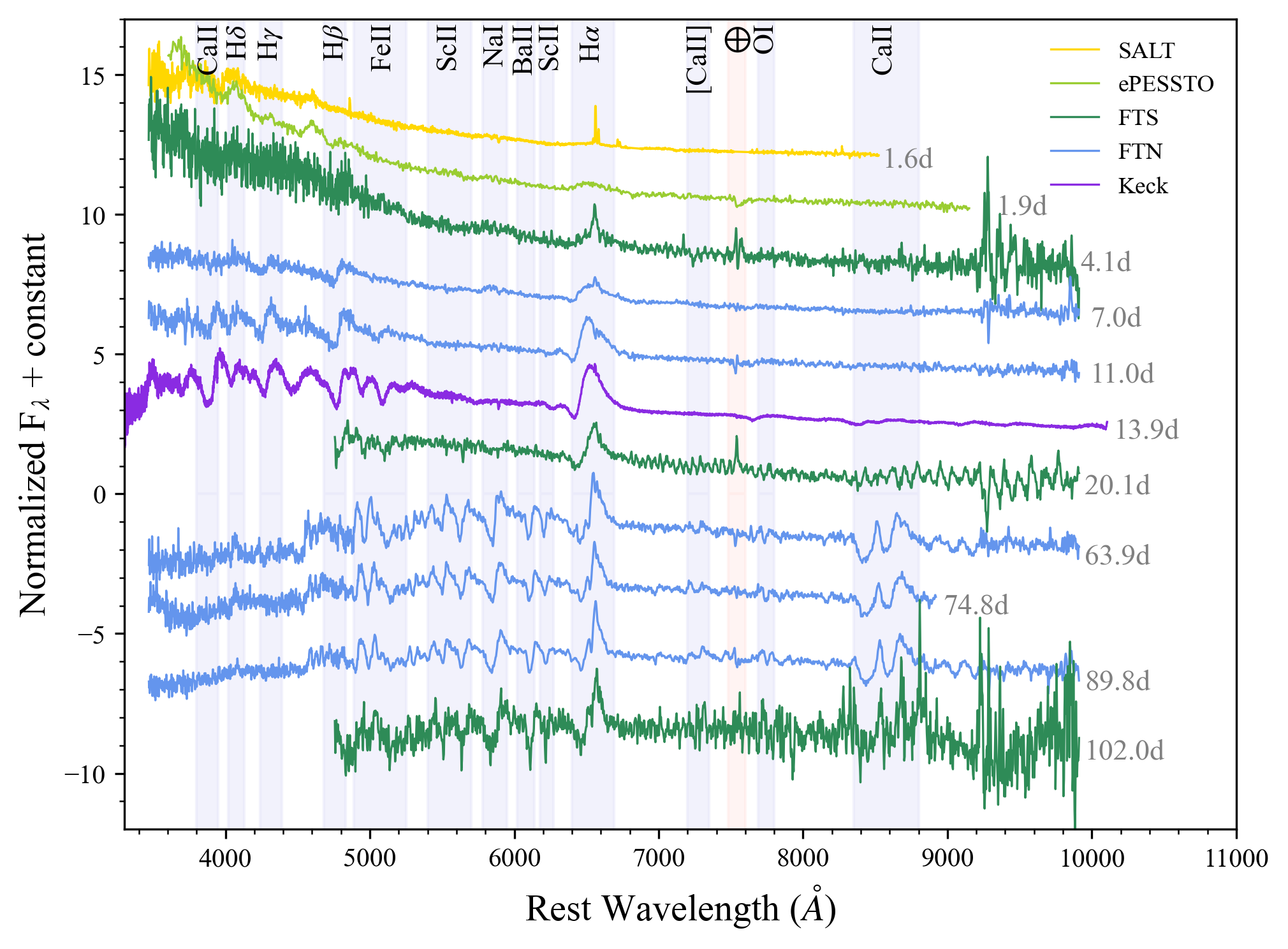
Figure 9: Spectroscopic evolution of SN 2018lab, corrected for $E(B-V)_{\mathrm{tot}}=0.22$. The early spectra ($\leq$7 days) of SN 2018lab are dominated by blue continua and H and He I emission lines. At 11 days, Ca II H&K and Fe II lines begin to appear. At later times ($>$50 days), more metal lines begin to appear: O I, Ca II infrared triplet, [Ca II], and Na ID. Strong Sc II and Ba II lines also emerge during this epoch. All of these spectral features and the timing of their emergence are typical of LLSNe (Pastorello et al., 2004; Spiro et al., 2014; Gutiérrez et al., 2017).

5 Spectral Evolution

The spectra $<$105 days post explosion of SN 2018lab are presented in Figure 9. Based on the 2D spectra, we attribute the narrow lines, particularly near H$\alpha$, to host contamination. While there could be narrow lines from the SN, we are unable to identify them given the nearby H II region.

The spectral evolution of SN 2018lab is similar to that of other LLSNe presented in previous papers (e.g. Benetti et al., 2001; Pastorello et al., 2004, 2009; Spiro et al., 2014; Takáts et al., 2014; Lisakov et al., 2017; Valerin et al., 2022). The first 4 spectra ($\leq$7 days) exhibit a blue continuum and the slow emergence of Balmer lines and He I $\lambda$5876, as is typical of all SNe II. These early lines have P Cygni profiles with very shallow absorption components. In the 11 day spectrum, the Ca II H&K ($\lambda$3934, $\lambda$3968) and the Fe II multiplet 42 ($\lambda$4924, $\lambda$5018, $\lambda$5169) lines become visible while He I $\lambda$5876 disappears. In the second half of the plateau ($>$50 days), the O I $\lambda$7774, Ca II infrared triplet ($\lambda$8498, $\lambda$8542, $\lambda$8662), [Ca II] ($\lambda$7291, $\lambda$7324), and Na ID ($\lambda$5890, $\lambda$5896) lines appear and strengthen. Further, this epoch also exhibits the characteristic strong Sc II and Ba II lines seen in LLSNe (Pastorello et al., 2004; Spiro et al., 2014; Gutiérrez et al., 2017).

There are a few notable features in the spectral evolution of SN 2018lab worth further discussion: the broad-lined flash feature in the early spectra, the appearance of an additional absorption component on the blue side of H$\alpha$, and the evolution of the H$\alpha$ profile in the second half of the plateau phase. These features are discussed in sections 5.1, 5.2, and 5.3 respectively.

5.1 Flash Spectroscopy

SN 2018lab does not exhibit narrow high-ionization lines in the early ($<$2 days) spectra. Instead, early spectra of SN 2018lab show a broad feature from 4500 to 4750 Å (see Figure 10). This feature peaks near the N V $\lambda$4604 line. The feature is most clear in the spectrum 1.9 days post-explosion though it is also present in the first spectrum of SN 2018lab (1.6 days post-explosion). The SN 2018lab spectrum from 4.1 days post-explosion has low signal-to-noise in the relevant wavelength range and we are unable to discern if the earlier broad feature remains. Only one LLSNe has exhibited narrow high-ionization lines, SN 2016bkv (Hosseinzadeh et al., 2018). In the spectra of SN 2016bkv, broad-lined flash features first appear in the spectra taken 4 days post-explosion in a shape similar to those seen in SN 2018lab, and the narrow lines become prominent a day later.

An early broad feature near 4600 Å, sometimes referred to as a “ledge” feature (Andrews et al., 2019; Soumagnac et al., 2020; Hosseinzadeh et al., 2022), has been observed in the early spectra of other SNe II (see Figure 10 and 11). Very few LLSNe have spectra $<$5 days following explosion. However of those that do—SN 2002gd (Spiro et al., 2014), SN 2005cs (Pastorello et al., 2006), SN 2010id (Gal-Yam et al., 2011), SN 2016bkv (Hosseinzadeh et al., 2018), and SN 2020cxd (Valerin et al., 2022)—the majority (SN 2005cs, SN 2010id, SN 2016bkv) appear to have a feature similar to what we observe for SN 2018lab (see Figure 10). The cause of this feature has been explained in three ways. In the spectra of SN 2005cs, Pastorello et al. (2006, their Fig. 5) interprets this feature as high velocity (HV) H$\beta$. There is no indication of a HV feature blueward of H$\alpha$ in SN 2018lab at early times, so we disfavor this explanation. An alternative explanation is provided for SN 2010id by Gal-Yam et al. (2011, their Fig. 2), which suggests that this feature is broad, blue-shifted He II $\lambda$4686. This analysis has been used to explain similar features in more typical SNe II as well, as seen in Quimby et al. (2007, their Fig. 10), Bullivant et al. (2018, their Fig. 20), and Andrews et al. (2019, their Fig. 18). The other interpretation is that the feature is the blend of several ionized features from the CSM (Dessart et al., 2017). This is the explanation used by Hosseinzadeh et al. (2018, their Fig. 2) to explain the shape of the feature in the spectra of SN 2016bkv, and has also explained similar features in more typical SNe II, as seen in Soumagnac et al. (2020, their Fig. 7), Bruch et al. (2021, their Fig. 5), and Hosseinzadeh et al. (2022, their Fig. 11). SN 2018lab’s early broad feature is somewhat double peaked indicating that there may be more than one line contributing to the feature. Therefore we posit that this feature is likely the blend of several ionized features from the CSM: N V, N III, C III, O III, and He II, rather than just blue-shifted He II (see Figure 10).

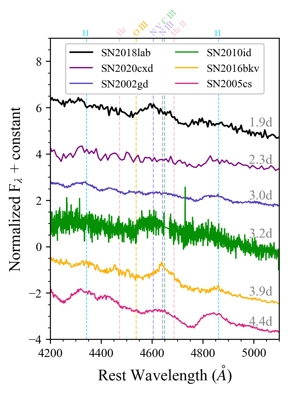
Figure 10: Comparison of the broad early feature seen in SN 2018lab with other LLSNe which have spectra $<$5 days post-explosion: SN 2002gd (Spiro et al., 2014), SN 2005cs (Pastorello et al., 2006, 2009), SN 2010id (Gal-Yam et al., 2011), SN 2016bkv (Hosseinzadeh et al., 2018), and SN 2020cxd (Valerin et al., 2022). Of these LLSNe, 4 (SN 2005cs, SN 2010id, SN 2016bkv, and SN 2018lab) out of the 6 have a strong broad early spectral feature near 4600 Å, though the shape, strength, and interpretation of this feature varies. It is likely that more LLSNe also exhibit similar features however a larger sample of early time ($<$5 days) spectra is needed to constrain the frequency at which this feature occurs. All spectra are extinction corrected.

The morphology of SN 2018lab’s ledge feature adds to the significant diversity observed in the early spectra of SNe II (see Figure 11). Symmetric narrow-lined flash features, like those seen in SN 2017ahn (Tartaglia et al., 2021) and SN 2020pni (Terreran et al., 2022) are produced via non-coherent scattering of thermal electrons. In contrast, bulk motions produce broad lines which can blend together and produce a broad asymmetric feature (Dessart et al., 2009). When observed, both narrow- and broad-lined flash features can be used as a probe of the properties of the progenitor and the extent of the CSM.

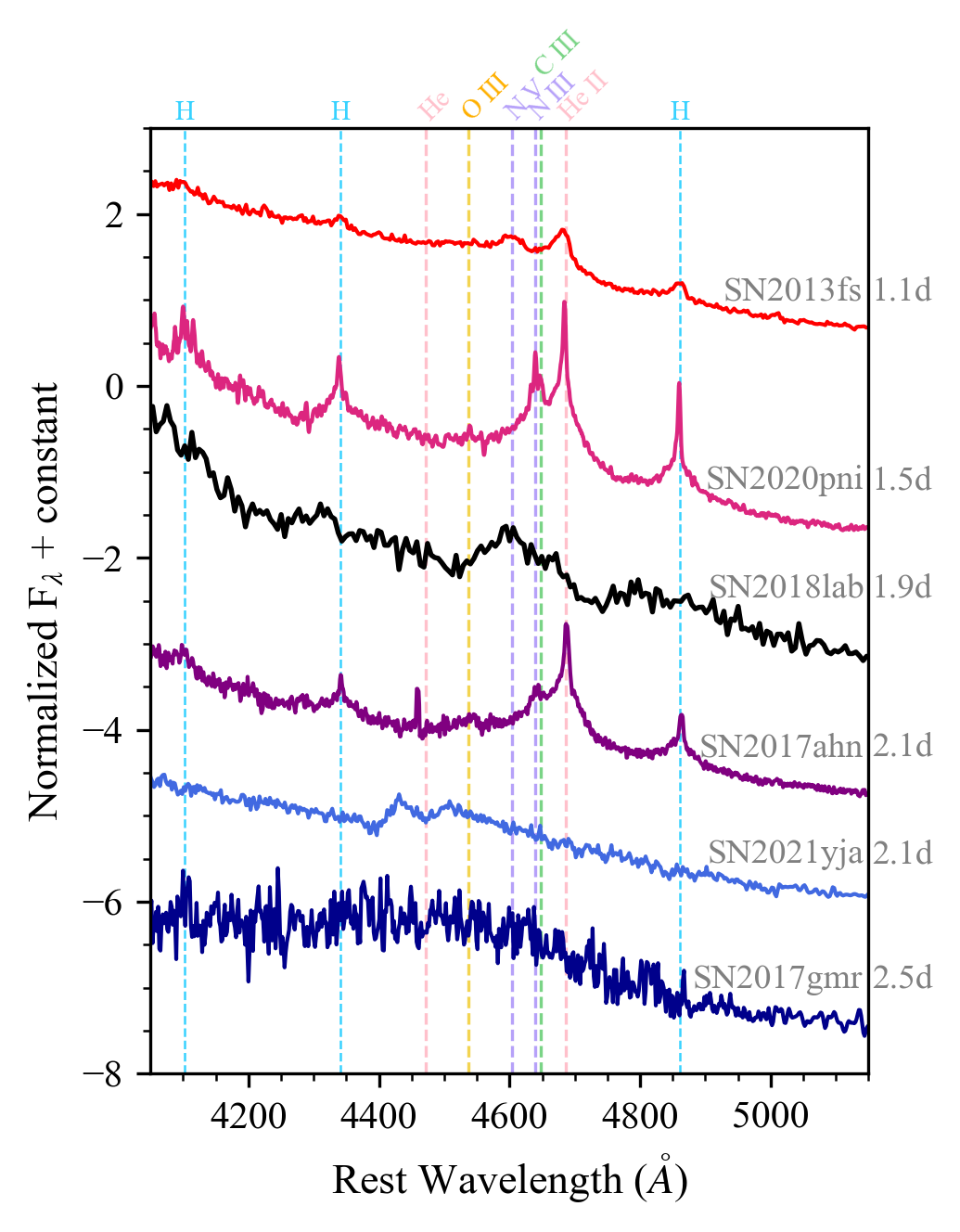
Figure 11: The 1.9 day spectrum of SN 2018lab compared to early time spectra of SN 2013fs (Bullivant et al., 2018), SN 2020pni (Terreran et al., 2022), SN 2017ahn (Tartaglia et al., 2021), SN 2021yja (Hosseinzadeh et al., 2022), and SN 2017gmr (Andrews et al., 2019). SN 2020pni and SN 2017ahn exhibit clear narrow-lined flash features; where as SN 2013fs, SN 2021yja, and SN 2017gmr all have broader early spectral features. The morphology of the feature in the spectra of SN 2018lab further highlights the significant diversity of flash spectroscopy observed in SNe II. All spectra have been corrected for extinction.

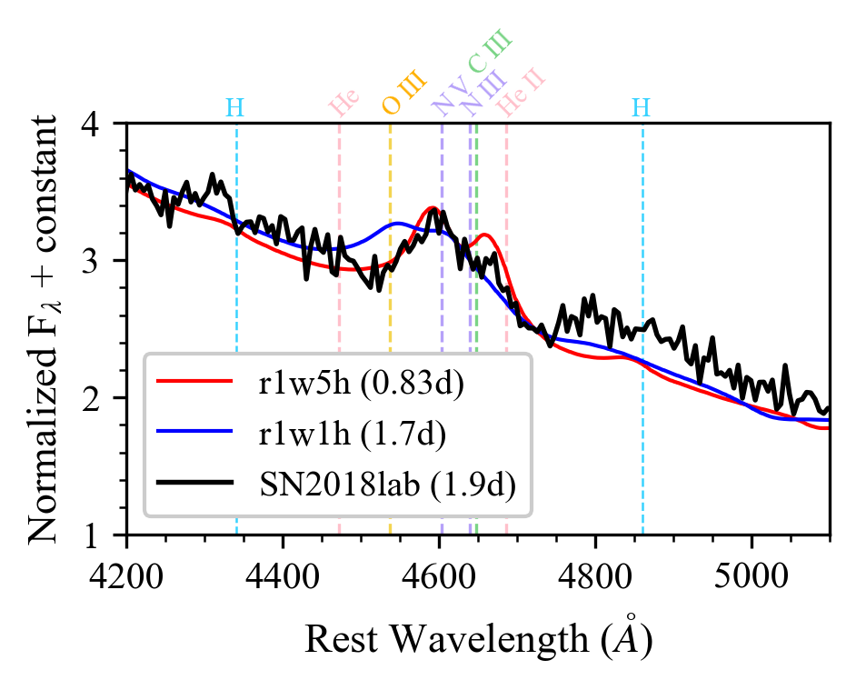
Figure 12: The early broad feature (4500-4750 Å) in the 1.9 day spectrum of SN 2018lab is compared to the Dessart et al. (2017) models that most closely resemble the spectra, r1w1h and r1w5h, which are both RSGs with extended atmospheres. The closest analogue to the SN 2018lab data is the the r1w5h model at 0.83 days. r1w1h and r1w5h are scaled by 70% to better fit the flux of the feature and have been convolved to the resolution of the observed spectrum (14 Å, Smartt et al., 2015).

As shown in Figure 12, the broad early spectral feature in the 1.9 day spectrum of SN 2018lab closely resembles the Dessart et al. (2017) r1w1h and r1w5h models, both of which have RSG progenitors with extended atmospheres and CSM. The correspondence with the r1w5h model is especially striking. The Dessart et al. (2017) r1w1 and r2w1 models also display ledge features, however these features are blue-shifted with respect to the observed SN 2018lab feature and are therefore not included in Figure 12.

Both the r1w1h and r1w5h models display narrow-lined flash features which appear immediately following explosion ($<$4 hrs) and quickly evolve into a broad spectral feature. These models focus on the first $\sim$15 days after explosion and only extend out to $1.5\times 10^{15}$ cm. Both r1w1h and r1w5h assume a progenitor star with a radius $R_{*}=501R_{\odot}$ and a wind mass loss rate of $10^{-6}$ and $5\times 10^{-3}$ $M_{\odot}\ \mathrm{yr}^{-1}$, respectively. Both have extended atmospheres, with scale heights of $H_{\rho}=0.3R_{*}$ for r1w1h and $H_{\rho}=0.1R_{*}$ for r1w5h. A moderate amount of energy deposited into an RSG envelope in late-stage nuclear burning can cause envelope expansion and mass ejection (Smith & Arnett, 2014; Morozova et al., 2020). Just like dense CSM, an extended envelope can produce excess luminosity in SNe light curves (Morozova et al., 2020). The shape of SN 2018lab’s early broad feature is qualitatively reproduced by the r1w1h and r1w5h models. Note that these models assume a much more energetic explosion ($1.35\times 10^{51}$ ergs) and a much more massive progenitor (ejecta mass of 12.52 $M_{\odot}$) than is typical for LLSNe, therefore the CSM around SN 2018lab is unlikely to have identical properties to the modeled CSM. However, the similarity of the observed ledge feature to that of the r1w1h and r1w5h models could indicate that the feature may be caused by an extended envelope of an RSG progenitor and CSM interaction.

The ledge feature seen in the SN 2018lab data is most similar to r1w5h at 0.83 days. The similarity to the r1w5h model suggests the presence of a higher density CSM than assumed by the r1w1h model, but still low enough to prevent the appearance of narrow-lined flash features more than a few hours after explosion. The early broad-lined flash features in the spectra of SN 2016bkv are also similar to the shape of the r1w5h model at 0.83 days. However, this spectral feature in SN 2016bkv appears 4 days post-explosion, substantially after the model epoch, which may suggest a much larger and denser CSM than described by the model (Hiramatsu et al., 2021a). In SN 2018lab, the features are present much earlier, indicating a progenitor with an extended envelope similar to that described by the r1w5h model with less dense CSM than SN 2016bkv.

5.2 Cachito Features

“Cachito” features (Gutiérrez et al., 2017) are small absorption features blueward of H$\alpha$ which are common in the optical spectra of SNe II (e.g. Bostroem et al., 2019, 2020; Dong et al., 2021). There are two main types of Cachito features, the kind which arise earlier ($<$40 days) in the spectral evolution and those which emerge later ($>$40 days). Both types of Cachito feature appear on the blue side of H$\alpha$ in the spectra of SN 2018lab, and are distinct (see Figure 13). Gutiérrez et al. (2017) found that, among SNe that exhibit Cachito features at $<$40 days post-explosion, in 60% of cases the feature results from Si II $\lambda 6355$ and the remaining cases are likely due to high velocity (HV) H$\alpha$. In SNe with Cachito features that emerge at $>$40 days, this feature may occur when X-rays from the SN shock ionize and excite the outer unshocked ejecta and HV H absorption forms (see Chugai et al., 2007).

The early Cachito feature, denoted as A in Figure 13, appears in the 11 and 13.9 day spectra at $13000-14000$ km s^-1 with respect to rest H$\alpha$. If the ‘A’ Cachito feature is due to Si II $\lambda 6355$ it should have a velocity similar to other metal lines in the spectrum (Gutiérrez et al., 2017). The measured velocity of the shallow ‘A’ Cachito feature in the 13.9 day spectrum of SN 2018lab is 4500 km s^-1 in the Si II $\lambda 6355$ rest frame. This velocity is similar to the velocity of Fe II $\lambda 5018$ and $\lambda 5169$ in the same epoch. We determine that the Cachito feature in the 11 and 13.9 day spectra of SN 2018lab is likely the result of Si II $\lambda 6355$.

The late Cachito feature, denoted as B in Figure 13, appears in the spectra from 50-90 days post explosion. While Ba II $\lambda 6497$ is visible in this region during the relevant epochs, a velocity analysis indicates that the ‘B’ Cachito feature in SN 2018lab is not associated with Si II $\lambda 6355$ or Ba II $\lambda 6497$. If the ‘B’ Cachito is related to HV H, its velocity should be similar to that of H$\alpha$ at earlier phases and a companion feature may be visible blueward of H$\beta$, though this is rare in the LLSNe subclass (Gutiérrez et al., 2017). The velocity relative to H$\alpha$ of the ‘B’ Cachito feature, $\sim$7500 km s^-1, is consistent with the velocity of H$\alpha$ in the 7 and 11 day spectra. This indicates that the Cachito feature in the 50-90 day spectra of SN 2018lab is likely the result of HV H. The numerous metal lines and low signal-to-noise on the blue end of the spectra make it difficult to discern if there is a counterpart HV feature near H$\beta$. This HV H feature is likely to be related to SN ejecta and RSG wind interaction (Gutiérrez et al., 2017) and may be further evidence for CSM surrounding the progenitor.

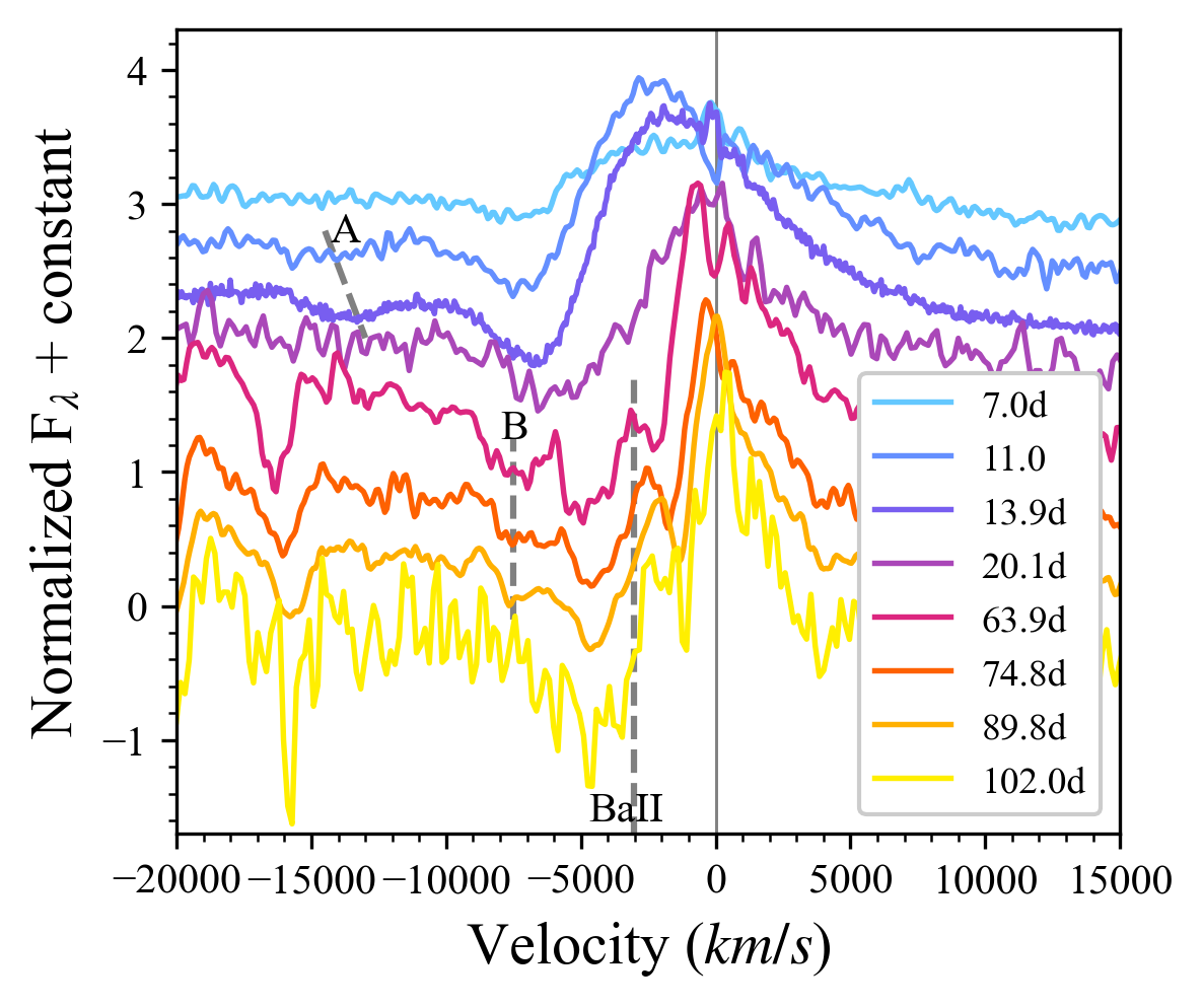
Figure 13: Evolution of H$\alpha$ starting at 7 days post-explosion. The spectra exhibit both A (10-15 days) and B (50-90 days) Cachito features (dotted lines). These features are likely due to Si II $\lambda 6355$ and HV H respectively. At $>50$ days the existence of a complex H$\alpha$ profile becomes evident. This is attributed to the presence of Ba II $\lambda 6497$ (rest-frame denoted with green dashed line).

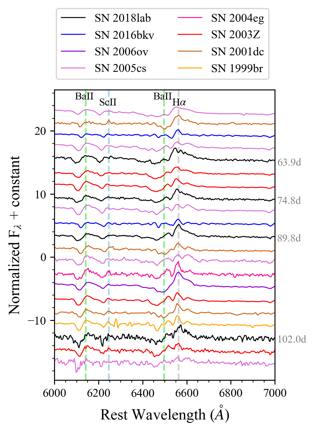
Figure 14: Spectra from the later half of the plateau phase of other notable LLSNe compared to SN 2018lab. Many LLSNe have strong Ba II and Sc II lines during this phase of evolution which yields a complex H$\alpha$ profile. Data taken from Pastorello et al. (2004, SN 1999br and SN 2001dc), Pastorello et al. (2009, SN 2005cs), Spiro et al. (2014, SN 2003Z, SN 2004eg, and SN 2006ov), Hosseinzadeh et al. (2018, SN 2016bkv). All spectra are corrected for extinction.

5.3 Complex H$\alpha$ Profile

The H$\alpha$ in SN 2018lab exhibits a clear P Cyngi profile beginning at the start of the plateau phase. In the spectra taken $7-20$ days post-explosion, the H$\alpha$ velocity is $6000-8000$ km s^-1. This is similar to the H$\alpha$ velocities observed for SN 2005cs at the same epochs (Pastorello et al., 2009). CSM interaction will decelerate SN ejecta, with high density CSM resulting in ejecta speeds $\sim$1000 km s^-1 slower than low density CSM in models of typical SNe II (Dessart et al., 2017). However, lower expansion speeds are characteristic of LLSNe and we are unable to set limits on the density of the CSM from this measurement alone.

The H$\alpha$ profile of SN 2018lab becomes complex starting in the 63.9 day spectrum, in the second half of the plateau phase (see Figure 13). This complex H$\alpha$ profile is not uncommon in LLSNe (see Figure 14) and has previously been described as the result of the combination of H$\alpha$ and Ba II $\lambda 6497$ (Benetti et al., 2001; Pastorello et al., 2009; Takáts et al., 2014; Lisakov et al., 2017; Valerin et al., 2022). The strength of Ba II lines in LLSNe is a temperature effect, rather than a relative overabundance. The low temperatures of LLSNe ejecta result in small Ba III/Ba II ratios and therefore strong Ba II lines (Turatto et al., 1998). The presence of exceptionally strong Ba II lines, particularly Ba II $\lambda 6142$, is a hallmark of the $\sim$80-100 day spectra of LLSNe (Pastorello et al., 2004; Spiro et al., 2014; Gutiérrez et al., 2017; Lisakov et al., 2018) and is also present in the spectra of SN 2018lab (see Figure 9).

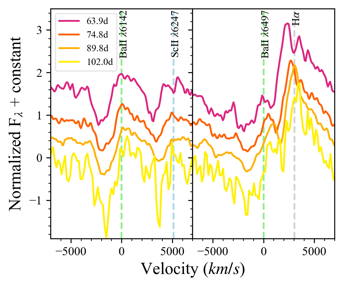
Figure 15: Evolution of the BaII $\lambda 6142$ and $\lambda 6497$ during the second half of the plateau phase ($\sim 50-100$ days). BaII $\lambda 6142$ has $v$(BaII)$\approx 2000$ km s^-1. BaII $\lambda 6497$ is likely to be evolving similarly to BaII $\lambda 6142$, therefore it is very difficult to determine the velocity of H$\alpha$ during these epochs. The relevant spectral lines (dotted) are at rest.

The velocity evolution of Ba II $\lambda 6142$ and $\lambda 6497$ is shown in Figure 15. The $v$(Ba II) of Ba II $\lambda 6142$, the strongest line in the Ba II multiplet which includes Ba II $\lambda 6497$, is $\sim 2000-1500$ km s^-1 for the $64-102$ day spectra of SN 2018lab. As expected, there is a clear absorption feature centered at $\sim 2000$ km s^-1 in the frame of Ba II $\lambda 6497$ as well. However, the profile of this region makes it difficult to determine the velocity of both Ba II $\lambda 6497$ and H$\alpha$ in the epochs where Ba II $\lambda 6497$ is present.

Higher signal-to-noise spectra of LLSNe within the crucial second half of the plateau phase are required in order to better understand the structure of the region surrounding H$\alpha$. Both SYNOW (Pastorello et al., 2004; Takáts et al., 2014) and CMFGEN (Lisakov et al., 2017, 2018) based models of LLSNe spectra fail to adequately replicate the H$\alpha$ profile. Barium (Ba) is an s-process element and is not included in current models. Detailed modeling, which includes Ba II, of the H$\alpha$ region in LLSNe is needed to facilitate a better understanding of the role of metals on the spectral evolution of LLSNe.

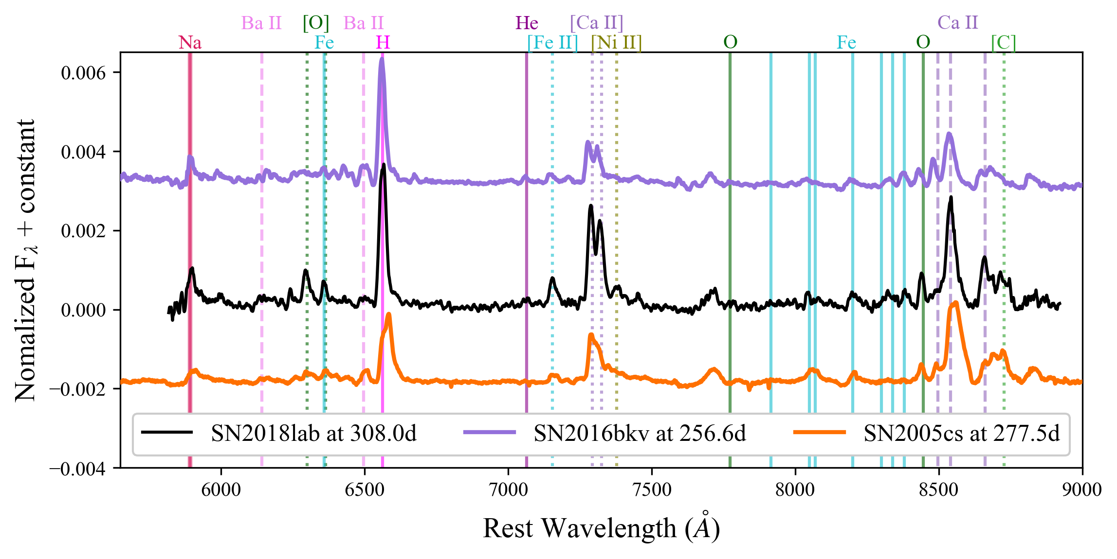
Figure 16: Late-time spectrum of SN 2018lab taken 308 days post explosion compared late time spectra of SN 2005cs (Pastorello et al., 2009) and SN 2016bkv (Hosseinzadeh et al., 2018). The spectrum of SN 2018lab is smoothed using a 10 pixel wide box kernel. All spectra are normalized to the total flux over the wavelength range of the observed SN 2018lab spectrum. While there are many similarities among all three spectra, [C I] $\lambda 8727$ is only present in the nebular spectra of SN 2005cs and SN 2018lab.

5.4 Nebular Spectra

Once SN ejecta are predominately transparent to optical light, several clues to the progenitor emerge in the nebular spectra. We obtained a nebular spectrum of SN 2018lab at 308 days post explosion. In Figure 16, the nebular spectrum of SN 2018lab is compared to similar spectral epochs of SN 2005cs (Pastorello et al., 2009), which has a confirmed low mass RSG progenitor, and SN 2016bkv (Hosseinzadeh et al., 2018), which has been suggested as a possible ECSN. The SN 2018lab spectrum presented in this figure has been smoothed using a 10 pixel wide box kernel to reduce the appearance of noise. While its nebular spectrum has many of the same features exhibited in both SN 2016bkv and SN 2005cs, SN 2018lab’s strong [C I] $\lambda 8727$ feature is only present in the nebular spectrum of SN 2005cs. The importance of this is explained below.

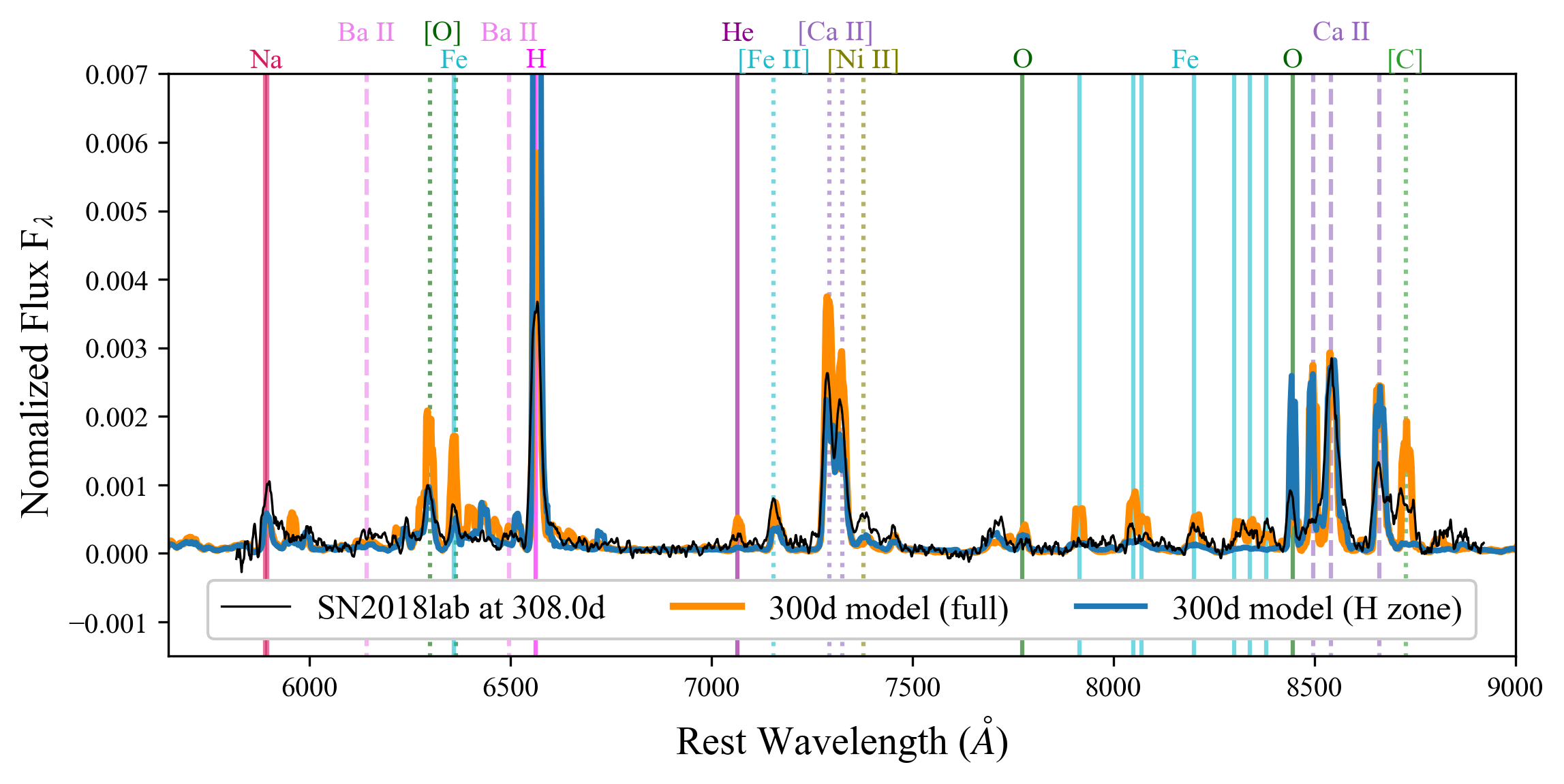
Figure 17: Late-time spectrum of SN 2018lab taken 308 days post explosion compared to the 9 M_⊙ Jerkstrand et al. (2018) models. Both the models and the spectrum are normalized to the total flux over the wavelength range of the observed spectrum to highlight line ratio differences. The full model, orange, is the expected spectrum for a iron CCSN. The hydrogen-zone model, blue, Jerkstrand et al. (2018) should be similar to the nebular spectrum expected of a ECSN. The late-time spectrum of SN 2018lab is similar to that of the iron core collapse model. In particular, [C I] $\lambda$8727 is present in the spectrum of SN 2018lab and is not included in the ECSNe model.

In Figure 17, the nebular spectrum of SN 2018lab is compared to the 300 day nebular spectra models for a 9 M_⊙ RSG progenitor presented in Jerkstrand et al. (2018). Since we are unable to determine the nickel mass of SN 2018lab and therefore can not correct for the nickel luminosity at this phase, these models and the spectrum are all normalized to the total flux over the wavelength range of the observed spectrum. The “pure hydrogen-zone” model presented in Jerkstrand et al. (2018) describes the signatures of a progenitor made up of only material from the hydrogen envelope (see their figure 2). While the H-zone model is not a electron-capture model, they expect a ECSN to resemble this model. The full Fe core-collapse model is distinctive from the H-zone model, particularly notable is the lack of He I $\lambda 7065$, Fe I $\lambda 7900-8500$, and [C I] $\lambda 8727$ in the H-zone model.

SN 2018lab clearly exhibits [C I] $\lambda 8727$ and several Fe I $\lambda 7900-8500$ lines. There is also some evidence of He I $\lambda 7065$. The appearance of these lines, though weaker than indicated by the model, strongly suggests the existence of He and O zones in the progenitor star at the time of collapse. This stellar composition indicates that SN 2018lab is likely to be the result of iron core-collapse in a red supergiant. Pre-explosion HST images of the IC 2163/NGC 2207 are unable to offer robust confirmation of this progenitor hypothesis. Given the distance to the host galaxy, the environment surrounding the SN, and the likelihood of a low mass progenitor star, further HST images of the site of SN 2018lab are required to shed light on the progenitor of SN 2018lab and the progenitors of LLSNe in general.

6 Summary & Conclusions

We present comprehensive photometric and spectroscopic observations of SN 2018lab. The early light curve of SN 2018lab is one of the best sampled SNe II to date due to the 30 minute cadence TESS light curve. The TESS light curve combined with extensive photometric and spectroscopic follow up places tight constraints on the early evolution and explosion epoch of SN 2018lab (see also the recent extensive follow-up campaign of the TESS-observed SN 2019esa; Andrews et al., 2022).

SN 2018lab is among the rare class of LLSNe with observational evidence of short-lived CSM interaction. First, the rising light curve can not be fit with an analytic model of shock cooling (Sapir & Waxman, 2017), indicating that the fast rise is likely the result of excess luminosity due to ejecta-CSM interaction, which is not accounted for in the model. Second, the flash spectroscopy in the first couple days following explosion reveals the presence of CSM around the progenitor star. In particular, the broad, ledge-shaped spectral feature at $\sim$4500–4750Å in the +1.9d spectrum of SN 2018lab is analogous to models of ejecta interaction of a RSG with an extended envelope and encompassed by close-in CSM (Dessart et al., 2017). While we do not explicitly rule out a super-AGB or high mass ($>20M_{\odot}$) RSG progenitor, the light curve shape and spectral evolution of SN 2018lab are similar to typical LLSNe, including SN 2005cs which has an identified low mass (10$\pm$3 M_⊙) RSG progenitor (Li et al., 2006). Further, the nebular spectrum of SN 2018lab displays many of the features expected to appear in the late-time spectra of iron CCSNe, adding to the likelihood of a RSG progenitor. Given the distance to the host and the nearby H II region, the pre-explosion HST images of SN 2018lab alone do not set strong enough limits to determine the progenitor of SN 2018lab. Additional post-explosion HST images taken after the SN light has sufficiently faded are required to set the robust constraints on the progenitor of SN 2018lab necessary to test the progenitor pathway suggested in this work.

Currently, there is no indication that the progenitor of SN 2018lab is not a RSG, suggesting that late stage mass loss may be common in LLSNe progenitors regardless if they are RSGs or super-AGBs. Evidence of CSM interaction alone is not enough to determine whether or not a LLSN is the result of electron-capture or core-collapse. Some work has been done to determine the characteristics which distinguish electron-capture from core-collapse processes, including line ratios in nebular spectra and progenitor identification (Hiramatsu et al., 2021a), but this is still in its early phases and uncertain. In order to truly understand the progenitor pathways of LLSNe, more spectra and photometry of these objects are urgently needed, not only following explosion but also during the nebular phase.

SN 2018lab is one of the few LLSNe with observed flash features. The increase in SNe II spectra taken in the hours and days following the explosion has uncovered the diverse morphology in broad early spectral features. Further early observations of SNe II, including the least luminous tails of the SNe II distribution, will shed light on the extent and mechanics of late stage mass loss in RSGs.

Acknowlegdements

We thank Luc Dessart for providing his model spectra. Time domain research by the University of Arizona team and D.J.S. is supported by NASA grant 80NSSC22K0167, NSF grants AST-1821987, 1813466, 1908972, & 2108032, and by the Heising-Simons Foundation under grant #2020-1864. J.E.A. is supported by the international Gemini Observatory, a program of NSF’s NOIRLab, which is managed by the Association of Universities for Research in Astronomy (AURA) under a cooperative agreement with the National Science Foundation, on behalf of the Gemini partnership of Argentina, Brazil, Canada, Chile, the Republic of Korea, and the United States of America. Research by Y.D., N.M., and S.V. is supported by NSF grants AST-1813176 and AST-2008108. K.A.B. acknowledges support from the DIRAC Institute in the Department of Astronomy at the University of Washington. The DIRAC Institute is supported through generous gifts from the Charles and Lisa Simonyi Fund for Arts and Sciences, and the Washington Research Foundation. The SALT data reported here were taken as part of Rutgers University program 2018-1-MLT-006 (PI: S. W. Jha). This research has made use of the NASA/IPAC Extragalactic Database (NED), which is funded by the National Aeronautics and Space Administration and operated by the California Institute of Technology. This research has also made use of the Spanish Virtual Observatory https://svo.cab.inta-csic.es) project funded by MCIN/AEI/10.13039/501100011033/ through grant PID2020112949GBI00 and the Weizmann Interactive Supernova Data Repository (WISeREP) (https://wiserep.weizmann.ac.il, Yaron & Gal-Yam, 2012). Based in part on data acquired at the Siding Spring Observatory 2.3 m, we acknowledge the traditional owners of the land on which the SSO stands, the Gamilaraay people, and pay our respects to elders past and present.

References

- Anderson et al. (2014) Anderson, J. P., González-Gaitán, S., Hamuy, M., et al. 2014, ApJ, 786, 67, doi: 10.1088/0004-637X/786/1/67
- Andrews et al. (2019) Andrews, J. E., Sand, D. J., Valenti, S., et al. 2019, ApJ, 885, 43, doi: 10.3847/1538-4357/ab43e3
- Andrews et al. (2022) Andrews, J. E., Pearson, J., Lundquist, M. J., et al. 2022, arXiv e-prints, arXiv:2205.12279. https://arxiv.org/abs/2205.12279
- Arnett (1982) Arnett, W. D. 1982, ApJ, 254, 1, doi: 10.1086/159698
- Astropy Collaboration et al. (2013) Astropy Collaboration, Robitaille, T. P., Tollerud, E. J., et al. 2013, A&A, 558, A33, doi: 10.1051/0004-6361/201322068
- Astropy Collaboration et al. (2018) Astropy Collaboration, Price-Whelan, A. M., Sipőcz, B. M., et al. 2018, AJ, 156, 123, doi: 10.3847/1538-3881/aabc4f
- Becker (2015) Becker, A. 2015, HOTPANTS: High Order Transform of PSF ANd Template Subtraction. http://ascl.net/1504.004
- Benetti et al. (1994) Benetti, S., Patat, F., Turatto, M., et al. 1994, A&A, 285, L13
- Benetti et al. (2001) Benetti, S., Turatto, M., Balberg, S., et al. 2001, MNRAS, 322, 361, doi: 10.1046/j.1365-8711.2001.04122.x
- Bostroem et al. (2019) Bostroem, K. A., Valenti, S., Horesh, A., et al. 2019, MNRAS, 485, 5120, doi: 10.1093/mnras/stz570
- Bostroem et al. (2020) Bostroem, K. A., Valenti, S., Sand, D. J., et al. 2020, ApJ, 895, 31, doi: 10.3847/1538-4357/ab8945
- Brown et al. (2007) Brown, P. J., Dessart, L., Holland, S. T., et al. 2007, ApJ, 659, 1488, doi: 10.1086/511968
- Brown et al. (2013) Brown, T. M., Baliber, N., Bianco, F. B., et al. 2013, PASP, 125, 1031, doi: 10.1086/673168
- Bruch et al. (2021) Bruch, R. J., Gal-Yam, A., Schulze, S., et al. 2021, ApJ, 912, 46, doi: 10.3847/1538-4357/abef05
- Bullivant et al. (2018) Bullivant, C., Smith, N., Williams, G. G., et al. 2018, MNRAS, 476, 1497, doi: 10.1093/mnras/sty045
- Callis et al. (2021) Callis, E., Fraser, M., Pastorello, A., et al. 2021, arXiv e-prints, arXiv:2109.12943. https://arxiv.org/abs/2109.12943
- Catchpole et al. (1987) Catchpole, R. M., Menzies, J. W., Monk, A. S., et al. 1987, MNRAS, 229, 15P, doi: 10.1093/mnras/229.1.15P
- Catchpole et al. (1988) Catchpole, R. M., Whitelock, P. A., Feast, M. W., et al. 1988, MNRAS, 231, 75P, doi: 10.1093/mnras/231.1.75P
- Chugai et al. (2007) Chugai, N. N., Chevalier, R. A., & Utrobin, V. P. 2007, ApJ, 662, 1136, doi: 10.1086/518160
- Chugai & Utrobin (2000) Chugai, N. N., & Utrobin, V. P. 2000, A&A, 354, 557. https://arxiv.org/abs/astro-ph/9906190
- Corgan et al. (2022) Corgan, A., Smith, N., Andrews, J., Filippenko, A. V., & Van Dyk, S. D. 2022, MNRAS, 510, 1, doi: 10.1093/mnras/stab2892
- Crawford et al. (2010) Crawford, S. M., Still, M., Schellart, P., et al. 2010, in Society of Photo-Optical Instrumentation Engineers (SPIE) Conference Series, Vol. 7737, Observatory Operations: Strategies, Processes, and Systems III, ed. D. R. Silva, A. B. Peck, & B. T. Soifer, 773725, doi: 10.1117/12.857000
- Davies & Dessart (2019) Davies, B., & Dessart, L. 2019, MNRAS, 483, 887, doi: 10.1093/mnras/sty3138
- Davis et al. (2021) Davis, S., Pessi, P. J., Fraser, M., et al. 2021, ApJ, 909, 145, doi: 10.3847/1538-4357/abdd36
- de Jaeger et al. (2019) de Jaeger, T., Zheng, W., Stahl, B. E., et al. 2019, MNRAS, 490, 2799, doi: 10.1093/mnras/stz2714
- de Vaucouleurs et al. (1991) de Vaucouleurs, G., de Vaucouleurs, A., Corwin, Herold G., J., et al. 1991, Third Reference Catalogue of Bright Galaxies (Springer), doi: 10.1007/978-1-4757-4363-0
- Dessart et al. (2009) Dessart, L., Hillier, D. J., Gezari, S., Basa, S., & Matheson, T. 2009, MNRAS, 394, 21, doi: 10.1111/j.1365-2966.2008.14042.x
- Dessart et al. (2017) Dessart, L., John Hillier, D., & Audit, E. 2017, A&A, 605, A83, doi: 10.1051/0004-6361/201730942
- Dong et al. (2021) Dong, Y., Valenti, S., Bostroem, K. A., et al. 2021, ApJ, 906, 56, doi: 10.3847/1538-4357/abc417
- Elmegreen et al. (1995a) Elmegreen, B. G., Sundin, M., Kaufman, M., Brinks, E., & Elmegreen, D. M. 1995a, ApJ, 453, 139, doi: 10.1086/176375
- Elmegreen et al. (2017) Elmegreen, D. M., Elmegreen, B. G., Kaufman, M., et al. 2017, ApJ, 841, 43, doi: 10.3847/1538-4357/aa6ba5
- Elmegreen et al. (2006) —. 2006, ApJ, 642, 158, doi: 10.1086/500966
- Elmegreen et al. (1995b) Elmegreen, D. M., Kaufman, M., Brinks, E., Elmegreen, B. G., & Sundin, M. 1995b, ApJ, 453, 100, doi: 10.1086/176374
- Elmegreen et al. (2001) Elmegreen, D. M., Kaufman, M., Elmegreen, B. G., et al. 2001, AJ, 121, 182, doi: 10.1086/318036
- Faran et al. (2014) Faran, T., Poznanski, D., Filippenko, A. V., et al. 2014, MNRAS, 442, 844, doi: 10.1093/mnras/stu955
- Fassia et al. (2001) Fassia, A., Meikle, W. P. S., Chugai, N., et al. 2001, MNRAS, 325, 907, doi: 10.1046/j.1365-8711.2001.04282.x
- Fazio et al. (2004) Fazio, G. G., Hora, J. L., Allen, L. E., et al. 2004, ApJS, 154, 10, doi: 10.1086/422843
- Filippenko (1997) Filippenko, A. V. 1997, ARA&A, 35, 309, doi: 10.1146/annurev.astro.35.1.309
- Filippenko et al. (2003) Filippenko, A. V., Chornock, R., Swift, B., et al. 2003, IAU Circ., 8159, 2
- Foreman-Mackey (2016) Foreman-Mackey, D. 2016, The Journal of Open Source Software, 1, 24, doi: 10.21105/joss.00024
- Foreman-Mackey et al. (2013) Foreman-Mackey, D., Hogg, D. W., Lang, D., & Goodman, J. 2013, PASP, 125, 306, doi: 10.1086/670067
- Förster et al. (2018) Förster, F., Moriya, T. J., Maureira, J. C., et al. 2018, Nature Astronomy, 2, 808, doi: 10.1038/s41550-018-0563-4
- Fraser et al. (2011) Fraser, M., Ergon, M., Eldridge, J. J., et al. 2011, MNRAS, 417, 1417, doi: 10.1111/j.1365-2966.2011.19370.x
- Gal-Yam et al. (2011) Gal-Yam, A., Kasliwal, M. M., Arcavi, I., et al. 2011, ApJ, 736, 159, doi: 10.1088/0004-637X/736/2/159
- Gal-Yam et al. (2014) Gal-Yam, A., Arcavi, I., Ofek, E. O., et al. 2014, Nature, 509, 471, doi: 10.1038/nature13304
- Galbany et al. (2016) Galbany, L., Hamuy, M., Phillips, M. M., et al. 2016, AJ, 151, 33, doi: 10.3847/0004-6256/151/2/33
- Gehrz et al. (2007) Gehrz, R. D., Roellig, T. L., Werner, M. W., et al. 2007, Review of Scientific Instruments, 78, 011302, doi: 10.1063/1.2431313
- González-Gaitán et al. (2015) González-Gaitán, S., Tominaga, N., Molina, J., et al. 2015, MNRAS, 451, 2212, doi: 10.1093/mnras/stv1097
- Groh et al. (2014) Groh, J. H., Meynet, G., Ekström, S., & Georgy, C. 2014, A&A, 564, A30, doi: 10.1051/0004-6361/201322573
- Gutiérrez et al. (2017) Gutiérrez, C. P., Anderson, J. P., Hamuy, M., et al. 2017, ApJ, 850, 89, doi: 10.3847/1538-4357/aa8f52
- Hamuy & Pinto (2002) Hamuy, M., & Pinto, P. A. 2002, ApJ, 566, L63, doi: 10.1086/339676
- Harris et al. (2020) Harris, C. R., Millman, K. J., van der Walt, S. J., et al. 2020, Nature, 585, 357, doi: 10.1038/s41586-020-2649-2
- Hiramatsu et al. (2021a) Hiramatsu, D., Howell, D. A., Van Dyk, S. D., et al. 2021a, Nature Astronomy, 5, 903, doi: 10.1038/s41550-021-01384-2
- Hiramatsu et al. (2021b) Hiramatsu, D., Howell, D. A., Moriya, T. J., et al. 2021b, ApJ, 913, 55, doi: 10.3847/1538-4357/abf6d6
- Hosseinzadeh & Gomez (2020) Hosseinzadeh, G., & Gomez, S. 2020, Light Curve Fitting, v0.2.0, Zenodo, Zenodo, doi: 10.5281/zenodo.4312178
- Hosseinzadeh et al. (2018) Hosseinzadeh, G., Valenti, S., McCully, C., et al. 2018, ApJ, 861, 63, doi: 10.3847/1538-4357/aac5f6
- Hosseinzadeh et al. (2022) Hosseinzadeh, G., Kilpatrick, C. D., Dong, Y., et al. 2022, arXiv e-prints, arXiv:2203.08155. https://arxiv.org/abs/2203.08155
- Huang et al. (2015) Huang, F., Wang, X., Zhang, J., et al. 2015, ApJ, 807, 59, doi: 10.1088/0004-637X/807/1/59
- Hunter (2007) Hunter, J. D. 2007, Computing in Science and Engineering, 9, 90, doi: 10.1109/MCSE.2007.55
- Jacobson-Galán et al. (2022) Jacobson-Galán, W. V., Dessart, L., Jones, D. O., et al. 2022, ApJ, 924, 15, doi: 10.3847/1538-4357/ac3f3a
- Jencson (2020) Jencson, J. E. 2020, PhD thesis, California Institute of Technology
- Jencson et al. (2017) Jencson, J. E., Kasliwal, M. M., Johansson, J., et al. 2017, ApJ, 837, 167, doi: 10.3847/1538-4357/aa618f
- Jencson et al. (2019) Jencson, J. E., Kasliwal, M. M., Adams, S. M., et al. 2019, ApJ, 886, 40, doi: 10.3847/1538-4357/ab4a01
- Jerkstrand et al. (2018) Jerkstrand, A., Ertl, T., Janka, H. T., et al. 2018, MNRAS, 475, 277, doi: 10.1093/mnras/stx2877
- Kasliwal et al. (2017) Kasliwal, M. M., Bally, J., Masci, F., et al. 2017, ApJ, 839, 88, doi: 10.3847/1538-4357/aa6978
- Kaufman et al. (2016) Kaufman, M., Elmegreen, B. G., Struck, C., et al. 2016, ApJ, 831, 161, doi: 10.3847/0004-637X/831/2/161
- Khazov et al. (2016) Khazov, D., Yaron, O., Gal-Yam, A., et al. 2016, ApJ, 818, 3, doi: 10.3847/0004-637X/818/1/3
- Kirshner et al. (1976) Kirshner, R. P., Arp, H. C., & Dunlap, J. R. 1976, ApJ, 207, 44, doi: 10.1086/154465
- Kitaura et al. (2006) Kitaura, F. S., Janka, H. T., & Hillebrandt, W. 2006, A&A, 450, 345, doi: 10.1051/0004-6361:20054703
- Kozyreva et al. (2022) Kozyreva, A., Janka, H.-T., Kresse, D., Taubenberger, S., & Baklanov, P. 2022, MNRAS, 514, 4173, doi: 10.1093/mnras/stac1518
- Leonard et al. (2000) Leonard, D. C., Filippenko, A. V., Barth, A. J., & Matheson, T. 2000, ApJ, 536, 239, doi: 10.1086/308910
- Li et al. (2006) Li, W., Van Dyk, S. D., Filippenko, A. V., et al. 2006, ApJ, 641, 1060, doi: 10.1086/499916
- Lisakov et al. (2017) Lisakov, S. M., Dessart, L., Hillier, D. J., Waldman, R., & Livne, E. 2017, MNRAS, 466, 34, doi: 10.1093/mnras/stw3035
- Lisakov et al. (2018) —. 2018, MNRAS, 473, 3863, doi: 10.1093/mnras/stx2521
- Lyman et al. (2014) Lyman, J. D., Levan, A. J., Church, R. P., Davies, M. B., & Tanvir, N. R. 2014, MNRAS, 444, 2157, doi: 10.1093/mnras/stu1574
- Maund et al. (2014) Maund, J. R., Reilly, E., & Mattila, S. 2014, MNRAS, 438, 938, doi: 10.1093/mnras/stt2131
- Maund & Smartt (2005) Maund, J. R., & Smartt, S. J. 2005, MNRAS, 360, 288, doi: 10.1111/j.1365-2966.2005.09034.x
- Menzies et al. (1987) Menzies, J. W., Catchpole, R. M., van Vuuren, G., et al. 1987, MNRAS, 227, 39P, doi: 10.1093/mnras/227.1.39P
- Morozova et al. (2020) Morozova, V., Piro, A. L., Fuller, J., & Van Dyk, S. D. 2020, ApJ, 891, L32, doi: 10.3847/2041-8213/ab77c8
- Morozova et al. (2017) Morozova, V., Piro, A. L., & Valenti, S. 2017, ApJ, 838, 28, doi: 10.3847/1538-4357/aa6251
- Morozova et al. (2018) —. 2018, ApJ, 858, 15, doi: 10.3847/1538-4357/aab9a6
- Munari & Zwitter (1997) Munari, U., & Zwitter, T. 1997, A&A, 318, 269
- Nakaoka et al. (2018) Nakaoka, T., Kawabata, K. S., Maeda, K., et al. 2018, ApJ, 859, 78, doi: 10.3847/1538-4357/aabee7
- Niemela et al. (1985) Niemela, V. S., Ruiz, M. T., & Phillips, M. M. 1985, ApJ, 289, 52, doi: 10.1086/162863
- Nomoto (1984) Nomoto, K. 1984, ApJ, 277, 791, doi: 10.1086/161749
- Oke et al. (1995) Oke, J. B., Cohen, J. G., Carr, M., et al. 1995, PASP, 107, 375, doi: 10.1086/133562
- Pastorello et al. (2004) Pastorello, A., Zampieri, L., Turatto, M., et al. 2004, MNRAS, 347, 74, doi: 10.1111/j.1365-2966.2004.07173.x
- Pastorello et al. (2006) Pastorello, A., Sauer, D., Taubenberger, S., et al. 2006, MNRAS, 370, 1752, doi: 10.1111/j.1365-2966.2006.10587.x
- Pastorello et al. (2009) Pastorello, A., Valenti, S., Zampieri, L., et al. 2009, MNRAS, 394, 2266, doi: 10.1111/j.1365-2966.2009.14505.x
- Pejcha & Prieto (2015) Pejcha, O., & Prieto, J. L. 2015, ApJ, 806, 225, doi: 10.1088/0004-637X/806/2/225
- Phillips et al. (2013) Phillips, M. M., Simon, J. D., Morrell, N., et al. 2013, ApJ, 779, 38, doi: 10.1088/0004-637X/779/1/38
- Pignata (2013) Pignata, G. 2013, in Massive Stars: From alpha to Omega, 176
- Poelarends et al. (2008) Poelarends, A. J. T., Herwig, F., Langer, N., & Heger, A. 2008, ApJ, 675, 614, doi: 10.1086/520872
- Pogge et al. (2010) Pogge, R. W., Atwood, B., Brewer, D. F., et al. 2010, in Society of Photo-Optical Instrumentation Engineers (SPIE) Conference Series, Vol. 7735, Ground-based and Airborne Instrumentation for Astronomy III, ed. I. S. McLean, S. K. Ramsay, & H. Takami, 77350A, doi: 10.1117/12.857215
- Poznanski et al. (2012) Poznanski, D., Prochaska, J. X., & Bloom, J. S. 2012, MNRAS, 426, 1465, doi: 10.1111/j.1365-2966.2012.21796.x
- Pumo et al. (2017) Pumo, M. L., Zampieri, L., Spiro, S., et al. 2017, MNRAS, 464, 3013, doi: 10.1093/mnras/stw2625
- Quimby et al. (2007) Quimby, R. M., Wheeler, J. C., Höflich, P., et al. 2007, ApJ, 666, 1093, doi: 10.1086/520532
- Razza et al. (2018) Razza, A., Pineda, J., Gromadzki, M., & Yaron, O. 2018, Transient Name Server Classification Report, 2018-2015, 1
- Richmond et al. (1994) Richmond, M. W., Treffers, R. R., Filippenko, A. V., et al. 1994, AJ, 107, 1022, doi: 10.1086/116915
- Ricker et al. (2015) Ricker, G. R., Winn, J. N., Vanderspek, R., et al. 2015, Journal of Astronomical Telescopes, Instruments, and Systems, 1, 014003, doi: 10.1117/1.JATIS.1.1.014003
- Rubin et al. (2016) Rubin, A., Gal-Yam, A., De Cia, A., et al. 2016, ApJ, 820, 33, doi: 10.3847/0004-637X/820/1/33
- Sand et al. (2018) Sand, D. J., Valenti, S., Lundquist, M., Amaro, R., & Wyatt, S. 2018, Transient Name Server Discovery Report, 2018-2000, 1
- Sanders et al. (2015) Sanders, N. E., Soderberg, A. M., Gezari, S., et al. 2015, ApJ, 799, 208, doi: 10.1088/0004-637X/799/2/208
- Sapir & Waxman (2017) Sapir, N., & Waxman, E. 2017, ApJ, 838, 130, doi: 10.3847/1538-4357/aa64df
- Schlafly & Finkbeiner (2011) Schlafly, E. F., & Finkbeiner, D. P. 2011, ApJ, 737, 103, doi: 10.1088/0004-637X/737/2/103
- Schlafly et al. (2010) Schlafly, E. F., Finkbeiner, D. P., Schlegel, D. J., et al. 2010, ApJ, 725, 1175, doi: 10.1088/0004-637X/725/1/1175
- Shivvers et al. (2015) Shivvers, I., Groh, J. H., Mauerhan, J. C., et al. 2015, ApJ, 806, 213, doi: 10.1088/0004-637X/806/2/213
- Smartt et al. (2009) Smartt, S. J., Eldridge, J. J., Crockett, R. M., & Maund, J. R. 2009, MNRAS, 395, 1409, doi: 10.1111/j.1365-2966.2009.14506.x
- Smartt et al. (2015) Smartt, S. J., Valenti, S., Fraser, M., et al. 2015, A&A, 579, A40, doi: 10.1051/0004-6361/201425237
- Smith et al. (2006) Smith, M. P., Nordsieck, K. H., Burgh, E. B., et al. 2006, in Society of Photo-Optical Instrumentation Engineers (SPIE) Conference Series, Vol. 6269, Society of Photo-Optical Instrumentation Engineers (SPIE) Conference Series, ed. I. S. McLean & M. Iye, 62692A, doi: 10.1117/12.672415
- Smith (2014) Smith, N. 2014, ARA&A, 52, 487, doi: 10.1146/annurev-astro-081913-040025
- Smith & Arnett (2014) Smith, N., & Arnett, W. D. 2014, ApJ, 785, 82, doi: 10.1088/0004-637X/785/2/82
- Smith et al. (2012) Smith, N., Cenko, S. B., Butler, N., et al. 2012, MNRAS, 420, 1135, doi: 10.1111/j.1365-2966.2011.20104.x
- Smith et al. (2015) Smith, N., Mauerhan, J. C., Cenko, S. B., et al. 2015, MNRAS, 449, 1876, doi: 10.1093/mnras/stv354
- Soumagnac et al. (2020) Soumagnac, M. T., Ganot, N., Irani, I., et al. 2020, ApJ, 902, 6, doi: 10.3847/1538-4357/abb247
- Spiro et al. (2014) Spiro, S., Pastorello, A., Pumo, M. L., et al. 2014, MNRAS, 439, 2873, doi: 10.1093/mnras/stu156
- Springob et al. (2005) Springob, C. M., Haynes, M. P., Giovanelli, R., & Kent, B. R. 2005, ApJS, 160, 149, doi: 10.1086/431550
- Struck et al. (2005) Struck, C., Kaufman, M., Brinks, E., et al. 2005, MNRAS, 364, 69, doi: 10.1111/j.1365-2966.2005.09539.x
- Suntzeff et al. (1988) Suntzeff, N. B., Hamuy, M., Martin, G., Gomez, A., & Gonzalez, R. 1988, AJ, 96, 1864, doi: 10.1086/114933
- Szalai et al. (2019) Szalai, T., Vinkó, J., Könyves-Tóth, R., et al. 2019, ApJ, 876, 19, doi: 10.3847/1538-4357/ab12d0
- Takáts et al. (2014) Takáts, K., Pumo, M. L., Elias-Rosa, N., et al. 2014, MNRAS, 438, 368, doi: 10.1093/mnras/stt2203
- Takáts et al. (2015) Takáts, K., Pignata, G., Pumo, M. L., et al. 2015, MNRAS, 450, 3137, doi: 10.1093/mnras/stv857
- Tartaglia et al. (2018) Tartaglia, L., Sand, D. J., Valenti, S., et al. 2018, ApJ, 853, 62, doi: 10.3847/1538-4357/aaa014
- Tartaglia et al. (2021) Tartaglia, L., Sand, D. J., Groh, J. H., et al. 2021, ApJ, 907, 52, doi: 10.3847/1538-4357/abca8a
- Terreran et al. (2022) Terreran, G., Jacobson-Galán, W. V., Groh, J. H., et al. 2022, ApJ, 926, 20, doi: 10.3847/1538-4357/ac3820
- Theureau et al. (2007) Theureau, G., Hanski, M. O., Coudreau, N., Hallet, N., & Martin, J. M. 2007, A&A, 465, 71, doi: 10.1051/0004-6361:20066187
- Tinyanont et al. (2022) Tinyanont, S., Ridden-Harper, R., Foley, R. J., et al. 2022, MNRAS, 512, 2777, doi: 10.1093/mnras/stab2887
- Tomasella et al. (2013) Tomasella, L., Cappellaro, E., Fraser, M., et al. 2013, MNRAS, 434, 1636, doi: 10.1093/mnras/stt1130
- Tsvetkov et al. (2006) Tsvetkov, D. Y., Volnova, A. A., Shulga, A. P., et al. 2006, A&A, 460, 769, doi: 10.1051/0004-6361:20065704
- Tsvetkov et al. (2018) Tsvetkov, D. Y., Shugarov, S. Y., Volkov, I. M., et al. 2018, Astronomy Letters, 44, 315, doi: 10.1134/S1063773718050043
- Turatto et al. (1998) Turatto, M., Mazzali, P. A., Young, T. R., et al. 1998, ApJ, 498, L129, doi: 10.1086/311324
- Valenti et al. (2014) Valenti, S., Sand, D., Pastorello, A., et al. 2014, MNRAS, 438, L101, doi: 10.1093/mnrasl/slt171
- Valenti et al. (2016) Valenti, S., Howell, D. A., Stritzinger, M. D., et al. 2016, MNRAS, 459, 3939, doi: 10.1093/mnras/stw870
- Valerin et al. (2022) Valerin, G., Pumo, M. L., Pastorello, A., et al. 2022, MNRAS, 513, 4983, doi: 10.1093/mnras/stac1182
- Vallely et al. (2021) Vallely, P. J., Kochanek, C. S., Stanek, K. Z., Fausnaugh, M., & Shappee, B. J. 2021, MNRAS, 500, 5639, doi: 10.1093/mnras/staa3675
- Van Dyk et al. (2003) Van Dyk, S. D., Li, W., & Filippenko, A. V. 2003, PASP, 115, 1, doi: 10.1086/345748
- Van Dyk et al. (2012) Van Dyk, S. D., Davidge, T. J., Elias-Rosa, N., et al. 2012, AJ, 143, 19, doi: 10.1088/0004-6256/143/1/19
- Virtanen et al. (2020) Virtanen, P., Gommers, R., Oliphant, T. E., et al. 2020, Nature Methods, 17, 261, doi: 10.1038/s41592-019-0686-2
- Werner et al. (2004) Werner, M. W., Roellig, T. L., Low, F. J., et al. 2004, ApJS, 154, 1, doi: 10.1086/422992
- Yaron & Gal-Yam (2012) Yaron, O., & Gal-Yam, A. 2012, PASP, 124, 668, doi: 10.1086/666656
- Yaron et al. (2017) Yaron, O., Perley, D. A., Gal-Yam, A., et al. 2017, Nature Physics, 13, 510, doi: 10.1038/nphys4025
- Yuan et al. (2016) Yuan, F., Jerkstrand, A., Valenti, S., et al. 2016, MNRAS, 461, 2003, doi: 10.1093/mnras/stw1419
- Zampieri et al. (1998) Zampieri, L., Colpi, M., Shapiro, S. L., & Wasserman, I. 1998, ApJ, 505, 876, doi: 10.1086/306192
- Zampieri et al. (2003) Zampieri, L., Pastorello, A., Turatto, M., et al. 2003, MNRAS, 338, 711, doi: 10.1046/j.1365-8711.2003.06082.x
- Zhang et al. (2020) Zhang, J., Wang, X., József, V., et al. 2020, MNRAS, 498, 84, doi: 10.1093/mnras/staa2273