Bayesian parameter estimation
for targeted anisotropic gravitational-wave background

Abstract

Extended sources of the stochastic gravitational backgrounds have been conventionally searched on the spherical-harmonics bases. The analysis during the previous observing runs by the ground-based gravitational-wave detectors, such as LIGO and Virgo, have yielded the constraints on the angular power spectrum $C_{\ell}$, yet it lacks the capability of estimating other parameters such as a spectral index. In this paper, we introduce an alternative Bayesian formalism to search for such stochastic signals with a particular distribution of anisotropies on the sky. This approach provides a Bayesian posterior of model parameters and also enables selection tests among different signal models. While the conventional analysis fixes the highest angular scale a priori, here we show a more systematic and quantitative way to determine the cutoff scale based on a Bayes factor, which depends on the amplitude and the angular scale of observed signals. Also, we analyze the third observing runs of LIGO and Virgo for the population of millisecond pulsars and obtain the 95 % constraints of the signal amplitude, $\epsilon<2.7\times 10^{-8}$.

I Introduction

Since the dawn of gravitational wave (GW) astronomy [1], a series of Gravitational Wave Transient Catalog (GWTC) published by the LIGO Scientific, Virgo and KAGRA Collaboration (LVK) [2, 3, 4, 5] have confirmed 90 GW signals in total from compact binary coalescences (CBCs) in the Universe. In upcoming observing runs by ground-based GW detectors, the detector network will be expanding with the Advanced Laser Interferometer Gravitational-wave Observatory (LIGO) [6] and Virgo [7] as well as KAGRA [8] and LIGO-India [9]. Additionally, the next generation of ground-based detectors such as the Einstein Telescope (ET) [10, 11, 12, 13] and the Cosmic Explorer (CE) [14] have been proposed to further increase the sensitivity to various types of GW sources.

A stochastic gravitational-wave background (SGWB) is the incoherent superposition of GWs emitted from many sources that are too faint to be resolved individually (see e.g., [15] for the detailed review). It is composed mainly of astrophysical sources such as binary black holes and binary neutron stars [16, 17, 18, 19, 20], supernovae [21, 22, 23, 24, 25], or ultralight bosons corotating around a black hole (BH) [26, 27, 28, 29, 30, 31]. Alternatively, cosmological sources can contribute to the SGWB, which include signals emitted during an inflationary era [32, 33, 34, 35, 36, 37, 38, 39, 40], phase transitions in the early Universe [41, 42, 43], and primordial BHs [44, 45, 46, 47]. These theoretical models, in general, predict a characteristic background amplitude, spectral shape or angular distribution [48, 49, 50, 51, 52, 53, 54, 55, 56, 57, 58, 59]. Therefore, one can not only detect but also, in principle, distinguish the different models by comparing these signatures in observed signals.

In contrast with established detections of CBCs, SGWBs have not yet been detected and hence it is one of the next milestones in the future observing runs. Conventional searches for a SGWB are mainly categorized into two types: isotropic [60, 61, 62, 63] and directional searches [64, 65, 66, 67, 68]. While the former assumes isotropic energy distribution of GWs over the sky and estimates the overall amplitude of the SGWB, the latter targets for its anisotropic distribution. Regarding the directional searches, two different methodologies have been adopted depending on signal models to pursue, e.g., using radiometer analyses [69, 70, 71] for pointlike sources or the spherical-harmonics decomposition (SHD) analysis [72] for extended sources.

Inspired by the SHD analysis approach, our work presented in this paper describes a Bayesian parameter estimation formalism targeted for an anisotropic distribution of GW energy. In the literature, similar targeted searches for different anisotropic sources have been introduced [73, 74], both of which construct the maximum-likelihood estimator of an overall amplitude of the GW energy density and provide its upper limit. Unlike these methods or the conventional SHD method which produces an estimator for each spherical-harmonics mode of the energy distribution, our formalism described here assumes an anisotropy model as known and infers other model parameters, e.g., an energy spectrum or an overall amplitude, through stochastic sampling. This can be seen as the extension of a parameter estimation for an isotropic background [75, 76] by adding higher spherical-harmonics modes in a signal model. As will be discussed in the rest of the paper, this also allows us to perform a selection across different anisotropy models and to optimize a spatial cutoff scale in the signal model.

This paper is structured as follows. First, Sec. II provides an overview of the conventional SHD analysis. Second, in Sec. III we describe our parameter estimation formalism based on the Bayesian framework. Following the procedure of data simulation and signal injection described in Sec. IV, from Sec. V to Sec. VII we show the results of various studies to assess the parameter inference consistency, the model selection and the optimization of the spatial cutoff scale. Subsequently, in Sec. VIII we analyze the real data from the third observing run (O3) by the Advanced LIGO and Virgo based on a population of millisecond pulsars (MSPs). Finally, in Sec. IX we discuss future prospects on the precision of parameter estimation and the constraints on model parameters by simulating several planned future detectors.

II Anisotropic stochastic gravitational wave background

The anisotropy of the SGWB can be expressed in terms of the dimensionless energy density $\Omega_{\mathrm{gw}}$ [77, 78, 15]

$$\Omega_{\mathrm{gw}}(f,\hat{\Omega})\equiv\frac{f}{\rho_{c}}\frac{\,\mathrm{d}^{3}\rho_{\mathrm{gw}}}{\,\mathrm{d}f\,\mathrm{d}^{2}\hat{\Omega}},$$ (1)

where $\,\mathrm{d}^{3}\rho_{\mathrm{gw}}$ is the GW energy per unit frequency $f$ and solid angle $\hat{\Omega}$, $\rho_{c}$ is the critical energy density required to have a spatially flat universe and $H_{0}$ is the Hubble constant. Assuming that $\Omega_{\mathrm{gw}}$ can be factorized into frequency and sky-direction dependent terms, i.e. $H(f)$ and $\mathcal{P}(\hat{\Omega})$ respectively, the above equation reads

$$\Omega_{\mathrm{gw}}(f,\hat{\Omega})=\frac{2\pi^{2}}{3H_{0}^{2}}f^{3}H(f)\mathcal{P}(\hat{\Omega}).$$ (2)

This assumption has been shown [78, 79] to hold across the frequency range in which LVK stochastic searches are most sensitive. Most of the literature adopts a power-law form for the frequency spectrum $H(f)=(f/f_{\mathrm{ref}})^{\alpha-3}$, for example, $\alpha=2/3$ as predicted for a CBC background [80]. This spectral model is used to perform a broadband search where one constructs sky maps by integrating different detector outputs over a broad range of frequencies.

For the sky-position dependent term $\mathcal{P}(\hat{\Omega})$, we apply the SHD,

$$\mathcal{P}(\hat{\Omega})=\sum_{\ell,m}\mathcal{P}_{\ell m}Y_{\ell m}(\hat{\Omega}),$$ (3)

where $Y_{\ell m}(\hat{\Omega})$ is a spherical-harmonics function evaluated at the sky position $\hat{\Omega}$. One uses the SHD to search for extended sources with a large angular scale. We first construct the dirty map $X_{\nu}$, which is essentially a cross-correlation between different detector outputs, and its covariance matrix $\Gamma_{\mu\nu}$ projected onto spherical-harmonics bases. We then produce a clean map as a nonbiased estimator of $\mathcal{P}_{\ell m}$, deconvolving the dirty map by the covariance matrix

$$\hat{\mathcal{P}}_{\mu}=\sum_{\nu}(\Gamma^{-1})_{\mu\nu}X_{\nu}.$$ (4)

Here $\mu,\nu$ subscripts represent a spherical-harmonics mode, i.e. $\mu\equiv(\ell,m)$, and $\Gamma^{-1}$ is the inverted covariance matrix.

To constrain anisotropies of a SGWB, we introduce the following estimator of the angular power spectrum

$$\hat{C_{\ell}}=\left(\frac{2\pi^{2}f^{3}_{\mathrm{ref}}}{3H_{0}^{2}}\right)^{2}\frac{1}{2\ell+1}\sum_{m}\left[|\hat{\mathcal{P}}_{\ell m}|^{2}-(\Gamma^{-1})_{\ell m,\ell^{\prime}m^{\prime}}\right],$$ (5)

which we compare to theoretical predictions.

III Formalism

III.1 Bayesian inference

Bayesian inference has been employed to estimate model parameters in the context of GW astronomy, such as signals from CBCs [81, 82, 83] and an isotropic GW background [75, 76]. The cross spectral density (CSD) at the frequency $f$ and the timestamp $t$ between outputs of the two detectors is defined as

$$C(f,t)\equiv\frac{2}{\tau}\tilde{s}_{1}(f,t)\tilde{s}_{2}^{*}(f,t)$$ (6)

where $\tilde{s}(f,t)$ is a short-term Fourier transform of the time series $s(t)$ within an interval $[t-\tau/2,t+\tau/2]$. Let the anisotropic background depend on a set of model parameters $\{\vec{\theta}\}$. In the presence of the anisotropic background, the CSD on a two-dimensional $(f,t)$ pixel map has the mean [72]

$$\langle C(f,t)\rangle=\gamma_{\mu}(f,t)\mathcal{P}_{\mu}(f,\{\vec{\theta}\}),$$ (7)

where $\gamma_{\mu}(f,t)$ denotes the overlap reduction function (ORF) [84] projected onto the spherical-harmonics basis represented by $\mu=(\ell,m)$ [79], and $\mathcal{P}_{\mu}(f,\{\vec{\theta}\})$ is a generic form of a spectral model with the anisotropic distribution. The Greek subscript implies the summation across the spherical-harmonics modes. The covariance of this CSD in the weak-signal approximation reads

$$\langle|C(f,t)|^{2}\rangle-|\langle C(f,t)\rangle|^{2}\approx\frac{P_{1}(f)P_{2}(f)}{\tau\Delta f},$$ (8)

where $P_{i}(f)$ is the power spectral density (PSD) of the $i$th detector and $\Delta f$ is the frequency resolution. Hence, these properties fully specify the Gaussian distribution, which represents the probability of obtaining the observable for a given signal model $\mathcal{M}$ and its relevant parameters, $p(\left\{C_{ft}\right\}\left|\{\vec{\theta}\};\mathcal{M}\right.)$. In the Bayesian context, this is equivalent to the likelihood and one aims to estimate the model parameters based on the posterior distribution

$$p\left(\left.\vec{\{\theta\}}\right|\{C_{f,t}\};\mathcal{M}\right)=\frac{p\left(\left\{C_{ft}\right\}\left|\{\vec{\theta}\};\mathcal{M}\right.\right)p(\vec{\{\theta\}})}{p(\left\{C_{ft}\right\}|\mathcal{M})},$$ (9)

where $p(\vec{\{\theta\}})$ is a prior distribution of the model parameters. Note that $p(\left\{C_{ft}\right\};\mathcal{M})$ in the denominator is called the Bayesian evidence

$$p(\left\{C_{ft}\right\}|\mathcal{M})=\int\bm{\,\mathrm{d}}\vec{\{\theta\}}p\left(\left\{C_{ft}\right\}\left|\{\vec{\theta}\};\mathcal{M}\right.\right)p(\vec{\{\theta\}}),$$ (10)

which is used for a selection test across different hypotheses [see Sec. VI].

III.2 $\mathcal{P}_{\ell m}$-specific Bayesian analysis

We further make several assumptions to simplify Eq. (7); First, we decouple the frequency dependence from the anisotropy of the signal model. Second, the only free parameter relevant to the anisotropy is its overall amplitude $\epsilon$. In other words, the signal model can be factorized as follows

$$\mathcal{P}_{\ell m}(f,\{\vec{\theta}\})=\epsilon\bar{H}(f;\{\vec{\theta^{\prime}}\})\bar{\cal P}_{\ell m},$$ (11)

where $\bar{H}(f;\{\vec{\theta^{\prime}}\})$ and $\bar{\cal P}_{\ell m}$ are normalized such that

$$\bar{H}(f;\{\vec{\theta^{\prime}}\})\equiv\frac{H(f;\{\vec{\theta^{\prime}}\})}{H(f_{\mathrm{ref}};\{\vec{\theta^{\prime}}\})},\qquad\bar{\cal P}_{\ell m}\equiv\frac{\mathcal{P}_{\ell m}}{\mathcal{P}_{00}}$$ (12)

respectively. Although one can relax these assumptions and consider a signal model with a more generic form, $\mathcal{P}_{\ell m}(f,\{\vec{\theta}\})$, in this paper we strict ourselves to this simplified case to perform $\mathcal{P}_{\ell m}$-specific Bayesian analysis so that $\mathcal{M}\rightarrow\bar{\cal P}_{\ell m}$, and leave its generalization as future work. Lastly, we set the cutoff on spatial scale characterized by $\ell_{\text{max}}$ and hence the subscript in Eq. (7) implies

$$\gamma_{\mu}(f,t)\mathcal{P}_{\mu}=\sum_{\ell=0}^{\ell_{\text{max}}}\sum^{\ell}_{m=-\ell}\gamma_{\ell m}(f,t)\mathcal{P}_{\ell m}.$$ (13)

With these assumptions, the likelihood obeys the Gaussian distribution as below

$$p\left(\left\{C_{ft}\right\}\left|\{\epsilon,\vec{\theta^{\prime}}\};\ell_{\text{max}},\bar{\cal P}_{\ell m}\right.\right)\propto\exp\left\{-\frac{1}{2}\sum_{f,t}\frac{\left|C(f,t)-\epsilon\bar{H}(f;\{\vec{\theta^{\prime}}\})\gamma_{\mu}(f,t)\bar{\cal P}_{\mu}\right|^{2}}{P_{1}(f,t)P_{2}(f,t)}\right\}.$$ (14)

Note that in the case of $\ell_{\text{max}}=0$, this likelihood expression reproduces the one for the isotropic stochastic background analysis [75, 76]. Also for the rest of this paper, the amplitude factor $\epsilon$ is normalized by $(\frac{2\pi}{3H_{0}^{2}}f_{\mathrm{ref}}^{3}\sqrt{4{\pi}})^{-1}$ so that this factor corresponds to $\hat{\Omega}_{0}$ in the isotropic search [60, 61, 62, 63]. Therefore, this formalism serves as a natural extension of parameter inference performed for the isotropic background.

While this formalism yields results dependent on a specific anisotropy modeled by $\bar{\cal P}_{\ell m}$, one can benefit from novel features as summarized below. First, the Bayesian evidence shown in Eq. (10) allows one to perform a model selection test by comparing those between different $\bar{H}(f;\{\vec{\theta^{\prime}}\})$ or $\bar{\cal P}_{\ell m}$ models. Second, the anisotropy model $\bar{\cal P}_{\ell m}$ also depends on the angular scale cutoff one imposes, and this can be optimized similarly by evaluating the Bayesian evidence across different $\ell_{\text{max}}$ values [see Sec. VII]. Third, since Eq. (14) essentially computes the residual in the CSD $C(f,t)$, the likelihood shown in Eq. (14) does not involve the inversion of a covariance matrix $\Gamma_{\mu\nu}$. In other words, this formalism is free from the regularization of an ill-conditioned covariance matrix, which otherwise would suffer from extra complexity just like the conventional SHD analysis [72].

For a given dataset and a signal model to recover, the pipeline stochastically samples over a multidimensional parameter space and iteratively evaluates the likelihood based on Eq. (14) for each sample until the posterior distribution can be sufficiently constructed. Regarding this implementation, we adopt a nested sampling algorithm Dynesty [85], implemented in the Bilby package. [82, 83]

IV Data simulation

The studies we conduct in the subsequent sections simulate a large set of noise data, e.g., the CSD $C(f,t)$, to assess statistical results. Here, we summarize our procedure of this data simulation and describe how it will be used for likelihood evaluation.

IV.1 Simulating noise data products

Given a set of the model parameters $\{\epsilon,\vec{\theta}\}$ and the signal model to recover, $\{\bar{H}(f;\{\vec{\theta^{\prime}}\}),\bar{\cal P}_{\mu}\}$, the full expression of Eq. (14) can be written as

$$2\ln\left[p\left(\left\{C_{ft}\right\}\left|\{\epsilon,\vec{\theta^{\prime}}\};\ell_{\text{max}},\bar{\cal P}_{\ell m}\right.\right)\right]=-\ln\left[(2\pi)^{d}|\Sigma_{CC^{\prime}}|\right]-\sum_{f,t}\left\{\frac{\tau\Delta f|C(f,t)|^{2}}{P_{1}(f,t)P_{2}(f,t)}\right\}+2\epsilon\mathrm{Re}[\bar{\cal P}_{\mu}^{*}X_{\mu}]-\epsilon^{2}\bar{\cal P}_{\mu}^{*}\Gamma_{\mu\nu}\bar{\cal P}_{\nu},$$ (15)

where $X_{\mu},\Gamma_{\mu\nu}$ are defined as

$$X_{\mu} =\sum_{f}\sum_{t}\gamma_{\mu}^{*}(f,t)\frac{\tau\Delta f\bar{H}(f;\{\vec{\theta^{\prime}}\})}{P_{1}(f,t)P_{2}(f,t)}C(f,t)$$ (16)

and

$$\Gamma_{\mu\nu} =\sum_{f}\sum_{t}\gamma_{\mu}^{*}(f,t)\frac{\tau\Delta f\bar{H}^{2}(f;\{\vec{\theta^{\prime}}\})}{P_{1}(f,t)P_{2}(f,t)}\gamma_{\nu}(f,t),$$ (17)

respectively. In the weak signal limit, the covariance matrix of the CSD, $\Sigma_{CC^{\prime}}$, can be approximated as a diagonal matrix whose elements are given by Eq. (8) with its dimension being

$$d=(\mathrm{\#\ of\ frequency\ bins})\times(\mathrm{\#\ of\ time\ segments}).$$ (18)

The likelihood in Eq. (15) is evaluated for a single baseline formed by a detector pair. For a general configuration of multiple baselines represented by $\bm{D}$, assuming uncorrelated noise among the detectors, the joint likelihood is given by a product of individual likelihood values computed for each distinct detector pair $\{IJ\}$

$$\begin{split}p&\left(\left\{C_{f,t}^{\bm{D}}\right\}\left|\{\epsilon,\vec{\theta^{\prime}}\};\ell_{\text{max}},\bar{\cal P}_{\ell m}\right.\right)=\\ &\qquad\qquad\prod_{I}\prod_{I>J}p\left(\left\{C_{f,t}^{IJ}\right\}\left|\{\epsilon,\vec{\theta^{\prime}}\};\ell_{\text{max}},\bar{\cal P}_{\ell m}\right.\right)\end{split}$$ (19)

Since the dirty map and the Fisher matrix need to be constructed based on Eqs. (16) and (17) every time a pipeline draws a parameter sample during its stochastic sampling process, the two-dimensional integration over frequencies and time segments can be a computational bottleneck. Hence, after synthesizing $C(f,t)$ based on the colored Gaussian noise, we precompute and store the time integration part in Eqs. (16) and (17), i.e.

$$X_{\mu} =\sum_{f}\bar{H}(f;\{\vec{\theta^{\prime}}\})\underbrace{\sum_{t}\frac{\tau\Delta f\gamma_{\mu}^{*}(f,t)C(f,t)}{P_{1}(f,t)P_{2}(f,t)}}_{\mathrm{precomputed}}$$ (20)

$$\Gamma_{\mu\nu} =\sum_{f}\bar{H}^{2}(f;\{\vec{\theta^{\prime}}\})\underbrace{\sum_{t}\frac{\tau\Delta f\gamma_{\mu}^{*}(f,t)\gamma_{\nu}(f,t)}{P_{1}(f,t)P_{2}(f,t)}}_{\mathrm{precomputed}},$$ (21)

including other static data products such as $|\Sigma_{CC^{\prime}}|$ and

$$\sum_{f,t}\left\{\frac{\tau\Delta f|C(f,t)|^{2}}{P_{1}(f,t)P_{2}(f,t)}\right\}.$$ (22)

IV.2 Signal injection

Following the pre-computation approach described above, we discuss how Eq. (15) should be modified in the presence of a background signal. Specifically, we consider the background signal which contributes to the CSD such that

$$C(f,t)=C_{n}(f,t)+\epsilon^{\mathrm{inj}}\bar{H}^{\mathrm{inj}}(f;\{\vec{\theta}^{\mathrm{inj}}\})\gamma_{\mu}(f,t)\bar{\cal P}^{\mathrm{inj}}_{\mu},$$ (23)

where $C_{n}(f,t)$ is the noise CSD with zero mean. After substituting Eq. (23) into Eq. (15) with some expansion, the following terms will appear in the likelihood

$$-2\epsilon^{\mathrm{inj}}\mathrm{Re}\left[(\bar{\cal P}^{\mathrm{inj}}_{\mu})^{*}X_{\mu}^{\mathrm{inj}}\right]-\left(\epsilon^{\mathrm{inj}}\right)^{2}(\bar{\cal P}^{\mathrm{inj}}_{\mu})^{*}\Gamma_{\mu\nu}^{\mathrm{inj}}\bar{\cal P}^{\mathrm{inj}}_{\nu}+2\epsilon\epsilon^{\mathrm{inj}}\mathrm{Re}\left[\bar{\cal P}^{*}_{\mu}\Gamma_{\mu\nu}^{(c)}\bar{\cal P}_{\nu}^{\mathrm{inj}}\right],$$ (24)

where $X^{\mathrm{inj}}_{\mu}$ and $\Gamma_{\mu\nu}^{\mathrm{inj}}$ follow the same definition as Eqs. (16) and (17) except replacing $\bar{H}(f;\{\vec{\theta^{\prime}}\})$ and $C(f,t)$ with $\bar{H}^{\mathrm{inj}}(f;\{\vec{\theta}^{\mathrm{inj}}\})$ and $C_{n}(f,t)$, respectively. We note that the last term in Eq. (24) involves the coupled Fisher matrix, which reads

$$\Gamma_{\mu\nu}^{(c)} =\sum_{f}\sum_{t}\gamma_{\mu}^{*}(f,t)\frac{\tau\Delta f\bar{H}\bar{H}^{\mathrm{inj}}}{P_{1}(f,t)P_{2}(f,t)}\gamma_{\nu}(f,t).$$ (25)

As we will describe in the subsequent section, the validity of this injection scheme can be shown by the statistical consistency in the injection recovery, e.g., Fig. 4.

V Statistical studies

In order to assess the statistical consistency of the injection recoveries, we perform injection campaigns using synthesized background signals with a specific anisotropy model, $\bar{{\cal P}}_{\ell m}$. To begin with, we summarize the setup of the injection set, simulated data, and the parameter inference. Finally, the implication from the injection campaigns will be described in Sec. V.3.

V.1 Setup

• Dataset:

  Following the procedure in Sec. IV, we simulate unfolded dataset for a one-year observation divided into 192-second segments with the frequency resolution of $0.25\text{\,}\mathrm{Hz}$ starting from $20\text{\,}\mathrm{Hz}$ to $500\text{\,}\mathrm{Hz}$. The CSD is produced from the cross-correlation between the two LIGO detectors with the projected O4 sensitivity ($\sim$$190\text{\,}\mathrm{M}\mathrm{p}\mathrm{c}$ of the binary inspiral range) shown in [86, 87].

• $\bar{\cal P}_{\ell m}$ model:

  As a toy model, we set $\bar{\cal P}_{\ell m}$ to be a mock Galactic plane shown in Fig. 1. When injecting and recovering this model, we adopt $\ell_{\text{max}}$ value consistent between the injection and recovery, ranging across 3, 5 and 7. We choose the highest $\ell_{\text{max}}=7$ because we find that the spherical-harmonics components above it only have negligible contribution to the total anisotropies. Also, note that the injected anisotropies with these $\ell_{\text{max}}$ values appear to be blurred compared to Fig. 1.

  

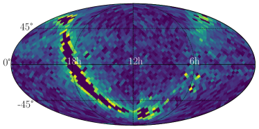
  Figure 1: Distribution of a mock Galactic plane visualized by Mollweide projection with HEALPix [88] pixelization of $n_{\mathrm{side}}=16$. The brighter color represents larger energy density.

• $\bar{H}(f)$ model:

  We assume $\bar{H}(f)$ is a simple power-law (PL) model, i.e.

  $$H_{\rm PL}(f;\alpha)=\left(\frac{f}{f_{\rm ref}}\right)^{\alpha-3}$$ (26)

  where $f_{\mathrm{ref}}=$25\text{\,}\mathrm{Hz}$$ and the “$-3$” in the exponent is added so that $\Omega_{\text{GW}}\propto f^{\alpha}$ [see Eq. (2)].

• Injections and prior distributions:

  Given the $\bar{H}(f)$ model above, the signal model has the two free parameters to infer, $(\epsilon,\alpha)$. In order to obtain a reasonable P-P plot, we adopt the same distributions consistently for both random draws of the injected parameters and the prior distributions of the same set of parameters for recovery as follows; for $\epsilon$, a log-uniform distribution in $10^{-8}$ to $10^{-5}$, and for $\alpha$, a Gaussian distribution with the mean of 5 and the standard deviation of 0.5. While the result of individual injection recoveries is found to be robust against changes in prior distributions, we select the above distributions so that most of the injections can be detected with great significance and their injected parameters are precisely inferred.

V.2 Injection recovery

We follow the injection scheme described in Sec. IV.2 and attempt to recover the injected values of the parameters by constructing the posterior distribution in the multidimensional parameter space. Here, we demonstrate two examples of injection recoveries performed with $\ell_{\text{max}}=7$. In one case, an injection is loud enough to be detected and the parameters are precisely inferred. Figure 2 shows that the both parameters of $(\log_{10}\epsilon,\alpha)$ are inferred to the precision of $0.01$ and the injected values (the red star) are located close to the bulk of the posterior samples, staying inside the 68% level of contours. As will be discussed later, the slight deviation of the injected values from the peak of the posterior distribution can be explained by the statistical error.

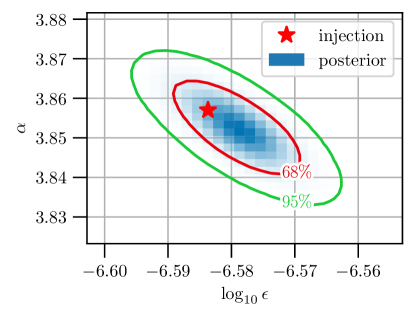
Figure 2: Posterior distribution for one of the detected injections. The injected values are $(\log_{10}\epsilon,\alpha)=(-6.584,3.857)$ and the BF is $\sim 24000$.

In contrast, the other case makes an injection with a smaller amplitude such that the injection is not recovered with sufficient significance and that instead the posterior distribution provides the constraints on the inferred parameters. Figure 3 indicates the excluded region of the two parameters outside the contours. We note that, in order to thoroughly cover the parameter space, the prior distribution for this particular injection recovery is chosen to be a log-uniform distribution from $10^{-13}$ to $10^{-5}$ for $\epsilon$, and a Gaussian distribution with the mean of 0 and the standard deviation of 3.5 for $\alpha$. The analysis with this configuration is performed separately from the setup described in Sec. V.1 for the purpose of demonstrating the parameter constraints.

Figure 3: Posterior distribution for one of the nondetected injections. The injected values are $(\log_{10}\epsilon,\alpha)=(-10.0,-2.5)$ and the BF is $\sim-0.35$.

V.3 Probability-probability plot

We perform 500 injection recoveries using $\bar{\cal P}_{\ell m},\bar{H}(f)$ models and the prior distributions described in Sec. V.1. Given the posterior samples of each recovery, we compute a percentile of the injected parameters with regard to the posterior probability. For example, if the injected values in Fig. 2 sit on the red contour, we would assign 68th percentile for the injection recovery. A collection of these percentiles in turn provides the cumulative fraction at each percentile value in the ascending order among the 500 injections. Eventually, we obtain the recovery database, each of which contains the percentile and the cumulative density. We plot them in Fig. 4, which is referred to as a probability-probability (P-P) plot. Since the posterior distributions without systematic error yield percentiles uniformly distributed between 0 and 1, a trace in the plot is expected to stay close to the diagonal with some statistical fluctuation. Figure 4 shows that the traces for all the three cases of $\ell_{\text{max}}=3,5,7$ stay within the 95% credible error region. This demonstrates the validity of data simulation, injection scheme and posterior construction. Throughout this study, we consistently use the same $\ell_{\text{max}}$ value for both the injection and its recovery. However, the $\ell_{\text{max}}$ value for the recovery can be different from that for the injection and we discuss the potential bias caused by the $\ell_{\text{max}}$ inconsistency in Appendix A.

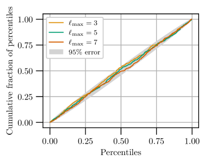
Figure 4: Probability-probability plot for 500 of the injection recoveries. Different colors indicate each value of $\ell_{\text{max}}=3,5,7$. The gray region is the 95% confidence region expected from the Poisson fluctuation.

VI Model selection

It is sometimes challenging to correctly interpret the underlying model from observed data. For instance, a broken power law (BPL) $\bar{H}(f;\{\vec{\theta^{\prime}}\})$ model with similar exponents could easily be mistaken by a simple PL model, especially for low signal-to-noise ratio (SNR). As mentioned in Sec. III.1, this formalism allows us to quantitatively compare the preference across multiple signal models. Here, we will demonstrate this aspect of the pipeline using toy models.

VI.1 Bayes factor

The fundamental tool to distinguish between two models within the Bayesian framework is the odds ratio. Given two models $\mathcal{M}_{1}$ and $\mathcal{M}_{2}$ and the data $D$, it is defined as

$$\mathcal{O}^{\mathcal{M}_{1}}_{\mathcal{M}_{2}}=\frac{p(\mathcal{M}_{1}|D)}{p(\mathcal{M}_{2}|D)}=\frac{p(D|\mathcal{M}_{1})}{p(D|\mathcal{M}_{2})}\frac{\pi(\mathcal{M}_{1})}{\pi(\mathcal{M}_{2})},$$ (27)

where $\pi(\mathcal{M}_{i})$ is the prior probability for model $\mathcal{M}_{i}$, $i=1,2$. Since, in our case, the prior odds for the both models are assumed to be equal, the odds ratio reduces to the BF,

$$\mathcal{B}^{\mathcal{M}_{1}}_{\mathcal{M}_{2}}=\frac{p(D|\mathcal{M}_{1})}{p(D|\mathcal{M}_{2})}.$$ (28)

We assess the statistical significance of a model relative to the other in terms of the BF. The evidence in favor of the model $\mathcal{M}_{1}$ is recognized to be strong around $\mathcal{B}^{\mathcal{M}_{1}}_{\mathcal{M}_{2}}\sim 10$ and decisive from $\sim 100$ [89].

Our tests proceed as follows: First, we synthesize the noise CSD from the cross-correlation between the two LIGO detectors with the projected O4 sensitivity. Then, we inject a signal simulated from a certain model $\mathcal{M}_{1}$ into the synthetic dataset. We recover it both with $\mathcal{M}_{1}$ and another model $\mathcal{M}_{2}$ involving different $\bar{H}(f)$ or $\bar{\cal P}_{\ell m}$ model. Finally, we compute the BF for different sets of injected parameters until we obtain a heatmap showing a distribution of the BF over the parameter space.

VI.2 $\bar{H}(f;\{\vec{\theta^{\prime}}\})$ model selection

The first case of the model selection studies tests under which conditions our pipeline is able to distinguish a BPL $\bar{H}(f;\{\vec{\theta^{\prime}}\})$ from a PL. While we follow the PL model shown in Eq. (26), $\bar{H}_{\rm BPL}(f)$ is defined, prior to the normalization in Eq. (12), as

$$\bar{H}_{\rm BPL}(f)\propto\left\{\begin{array}[]{cc}(f/f_{0})^{\alpha_{1}-3}&\text{if }f<f_{0}\\ (f/f_{0})^{\alpha_{2}-3}&\text{if }f\geq f_{0}\end{array}\right..$$ (29)

We model the BPL case with four free parameters, i.e. three of them from $\bar{H}_{\mathrm{BPL}}(f)$ as well as the overall amplitude parameter, $\epsilon$. An example posterior is shown in Fig. 5. For this analysis, we inject the BPL model with $\alpha_{1}=2/3$ and $f_{0}=100$ Hz fixed, hence exploring the $(\epsilon,\alpha_{2})$ parameter space. We adopt the prior distributions for each parameter as follows; for $\epsilon$, a log-uniform distribution from $10^{-12}$ to $10^{0}$, for $\alpha_{1}$ and $\alpha_{2}$, a Gaussian distribution with the mean of 0 and the standard deviation of 3.5, and for $f_{0}$, a uniform distribution in $20\text{\,}\mathrm{Hz}$ and $500\text{\,}\mathrm{Hz}$. The $\bar{\cal P}_{\ell m}$ model is taken as the the sky distribution of the Galactic plane shown in Fig. 1 with $\ell_{\text{max}}=7$.

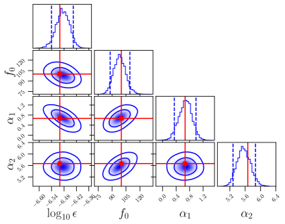
Figure 5: Example posterior of an injection recovery based on the BPL model, with $\ln\mathcal{B}^{\rm BPL}_{\rm PL}=417$. The recovery is consistent with the injection, indicated by the red markers and lines.

The heatmap in Fig. 6 suggests that higher values of $\epsilon$ result in the identification of the correct model with greater significance, transitioning around $\epsilon\sim 10^{-7}-10^{-6}$. The BF tends to increase for higher values of $\alpha_{2}$. Also expectedly, the gap in $\alpha_{2}=2/3$ is observed because this is equal to the fixed value of $\alpha_{1}$, in which case the BPL model becomes completely degenerated with a PL of $\alpha=2/3$, leading to the equal odds between the two models $\mathcal{B}^{\rm BPL}_{\rm PL}\sim 1$.

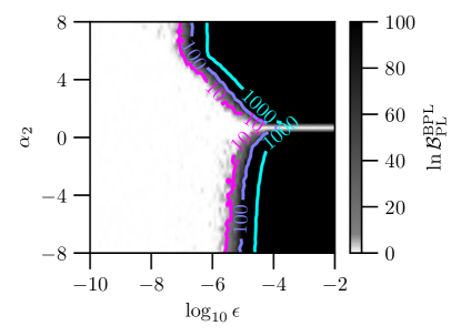
Figure 6: Heatmap showing the BF for the BPL vs PL $\bar{H}(f)$ recovery models across grids of $\epsilon$ and $\alpha_{2}$ values for injected BPL $\bar{H}(f)$ with $f_{0}=100$ Hz, $\alpha_{1}=2/3$.

VI.3 $\bar{\cal P}_{\ell m}$ model selection

Similar to the study summarized above, here we compare two different $\bar{\cal P}_{\ell m}$ models, fixing $\bar{H}(f)$ to be a PL model. We do not introduce any new free parameter in $\bar{\cal P}_{\ell m}$ and explore only the ($\epsilon,\alpha$) parameter space.

To demonstrate the capability of $\bar{\cal P}_{\ell m}$ model selection, we inject a background signal of the Galactic plane $\bar{\cal P}_{\ell m}$ with $\ell_{\text{max}}=7$ and identify the parameter space where one can distinguish it from purely isotropic model, i.e. $\bar{\cal P}_{\ell m}=0$ if $\ell\neq 0$ or $m\neq 0$. We note that given the normalization, an arbitrary $\bar{\cal P}_{\ell m}$ skymap with $\ell=0$ reduces to an isotropic model. We explore different injected values over the $(\epsilon,\alpha)$ parameter space, obtaining the heatmap shown in Fig. 7. The heatmap indicates that the analysis prefers the Galactic plane $\bar{\cal P}_{\ell m}$ model at around $\epsilon=10^{-6}$ in the most conservative case, similar to the previous study. This threshold decreases for high values of $\alpha$, which enhance the signal for high frequencies. Hence, for the darker part of the parameter space, the pipeline is capable of detecting the signature of higher-order spatial modes and distinguishing it from the isotropic background.

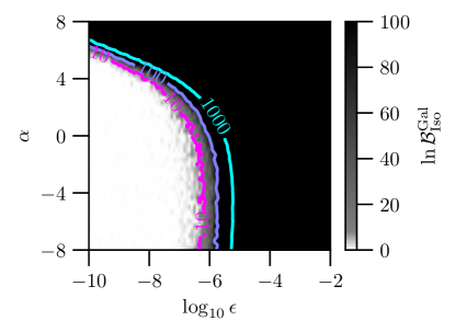
Figure 7: Heatmap showing the BF for the Galactic plane vs isotropic $\bar{\cal P}_{\ell m}$ recovery models across grids of $\epsilon$ and $\alpha$ values for injected Galactic plane $\bar{\cal P}_{\ell m}$ model.

VII $\ell_{\mathrm{max}}$ optimization

As mentioned in Sec. III.2, the likelihood in our formalism involves the angular scale cutoff, $\ell_{\text{max}}$ as a hyperparameter to be tuned. The study in Appendix A suggests the systematic bias in the parameter inference due to potential mismatch in $\ell_{\text{max}}$ value. Also, it has been known that unreasonably high $\ell_{\text{max}}$ causes overfitting to observed data, and thus several approaches have been taken to optimize the $\ell_{\text{max}}$ value. In the conventional SHD analysis [see e.g., [61]], the $\ell_{\text{max}}$ value is chosen in the consideration of the diffraction limit. However, this reasoning can be established only for a two-detector configuration, and also the $\ell_{\text{max}}$ choice depends on the shape of a signal spectrum, e.g., the power-law index of $\bar{H}(f)$. Floden et al. [90] further investigated this in the case of a pointlike source with different signal amplitudes. The authors found that the larger $\ell_{\text{max}}$ yields greater localization of the source, while the smaller $\ell_{\text{max}}$ tends to recover larger SNR. This indicates the potential sweet spot of the $\ell_{\text{max}}$ that compromises between the angular resolution and the signal detection, although the optimal choice potentially depends on the signal amplitude in the data. They also suggested that, for sufficiently loud signals, the $\ell_{\text{max}}$ value can possibly surpass the one predicted from the diffraction limit argument. Yet, their conclusion cannot be directly applied to extended source models, which we consider in this work. Here, we describe a more generic and quantitative method to optimize the choice of $\ell_{\text{max}}$ based on the Bayesian framework.

VII.1 Method

Thrane et al. [72] first discussed the approach to assess the validity of a chosen $\ell_{\text{max}}$ by computing the Bayesian evidence given by

$$p(\left\{C_{ft}\right\}|\ell_{\text{max}})=\int\bm{\,\mathrm{d}}\bar{\cal P}_{\ell m}\ p\left(\left\{C_{ft}\right\}\left|\bar{\cal P}_{\ell m};\ell_{\text{max}}\right.\right)p(\bar{\cal P}_{\ell m}).$$ (30)

Although this approach can be applied, in principle, for arbitrary signal models or amplitudes, the number of marginalized parameters, which scales with $(\ell_{\text{max}}+1)^{2}$, makes it practically unfeasible to evaluate the integration above with sufficient precision within a reasonable timescale. Instead, in the $\bar{\cal P}_{\ell m}$-specific analysis, the Bayesian evidence is computed for a fixed $\bar{\cal P}_{\ell m}$ model as well as $\ell_{\text{max}}$ by marginalizing over only the model parameters, $\{\vec{\theta}\}$, which do not necessarily involve high dimensionality [see Eq. (10)].

Subsequently, we evaluate the odds ratio of a signal hypothesis ($\mathcal{S}$) over the noise hypothesis ($\mathcal{N}$), which reads as a function of $\ell_{\text{max}}$

$$\mathcal{O}^{\mathcal{S}}_{\mathcal{N}}(\ell_{\text{max}}) =\frac{p(\mathcal{S},\ell_{\text{max}}|\{C_{ft}\})}{p(\mathcal{N}|\{C_{ft}\})}$$ (31)

$$=\frac{p(\{C_{ft}\}|\mathcal{S},\ell_{\text{max}})}{p(\{C_{ft}\}|\mathcal{N})}\frac{\pi(\mathcal{S},\ell_{\text{max}})}{\pi(\mathcal{N})}.$$ (32)

Following the methodology in Sec. VI.1, we assign equal prior odds to each signal and noise hypothesis and hence only consider the BF

$$\mathcal{B}^{\mathcal{S}}_{\mathcal{N}}(\ell_{\text{max}})=\frac{p(\{C_{ft}\}|\mathcal{S},\ell_{\text{max}})}{p(\{C_{ft}\}|\mathcal{N})}$$ (33)

as the deciding factor. We note that the evidence for the noise hypothesis is given by the likelihood without any signal component subtracted, i.e. its exponent proportional to Eq. (22). Since the Bayesian evidence quantifies the degree to which the real signal in the data can be described by the recovered signal model, we identify the $\ell_{\text{max}}$ that maximizes $\mathcal{B}^{\mathcal{S}}_{\mathcal{N}}$ as its optimal choice.

VII.2 Results

We conduct a series of simulations using four kinds of the 1-year synthesized data with the projected O4 sensitivity as described in Sec. V.1. Three of them include a signal injection based on the PL $\bar{H}(f)$ ($f_{\mathrm{ref}}=$25\text{\,}\mathrm{Hz}$$ and $\alpha=4$) and the Galactic plane $\bar{\cal P}_{\ell m}$ model shown in Fig. 1 with the injected $\ell_{\text{max}}=7$ and increasing amplitudes of $\epsilon=10^{-8},10^{-7},10^{-6}$. The four datasets are analyzed by recovering the signal model consistent with the injection while varying $\ell_{\text{max}}$ values from 0 to 10 for each dataset. For the parameter estimation, we take $(\epsilon,\alpha)$ as free parameters to infer and set their priors as a log-uniform distribution from $10^{-13}$ to $10^{-5}$ and a Gaussian distribution with the mean of 0 and the standard deviation of 3.5, respectively.

For each dataset and the $\ell_{\text{max}}$ value for recovery, the same analysis is repeated using 10 different realizations of the noise data and the BF is computed each time. Figure 8 shows its mean and 1-sigma error bar as a function of the recovered $\ell_{\text{max}}$. We find that the BF in log scale overall scales with roughly $\epsilon^{2}$ as expected from Eq. (14), and its peak is located at the $\ell_{\text{max}}$ value consistent with the injection ($\ell_{\text{max}}=7$ indicated by the black dashed line) for all the three datasets. The BF for the noninjection dataset, on the other hand, does not indicate any significant detection and show a relatively flat structure across the recovered $\ell_{\text{max}}$ values. Also, we note that the error bars tend to reduce relative to the mean for larger signal amplitudes. This observation implies that the optimal $\ell_{\text{max}}$ is determined by the cutoff scale of the background signal present in data and that its significance increases with the signal amplitude.

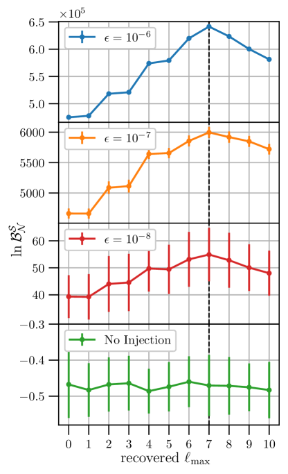
Figure 8: Recovered BFs as a function of recovery $\ell_{\text{max}}$. Different colors represent each magnitude of the background injection, $\epsilon=10^{-6},10^{-7},10^{-8}$ and no injection. The dashed black line at $\ell_{\text{max}}=7$ is the $\ell_{\text{max}}$ used for the injected signal model.

VIII O3 MSP analysis

As an example of astrophysically motivated analyses beyond the toy models we described so far, we adopt a MSP $\bar{\cal P}_{\ell m}$ model and search for the signal model using the publicly available data [91] from O3 of the LVK. We apply the same preprocessing and gating to the O3 timeseries data collected from the two LIGO and Virgo detectors as described in [67], resulting in the CSD with different livetime for each detector pair (i.e. 169 days for HL, 146 days for HV and 153 days for LV baseline respectively). Subsequently, the CSD is folded to one sidereal day using the method in [92], and the static data products are computed by the PyStoch pipeline [93, 94] and stored following the procedure similar to Sec. IV.1.

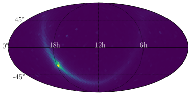
Figure 9: Distribution of the MSP population visualized by Mollweide projection with HEALPix [88] pixelization of $n_{\mathrm{side}}=16$. The brighter color represents larger energy density.

Previously, similar searches for the MSPs were conducted based on the isotropic [95] or targeted [73] analysis. The both searches provide the upper limit on averaged ellipticity of the MSP population and the number of MSPs in the observed frequency band. Regarding the MSP population in our analysis, we adopt the $\bar{\cal P}_{\ell m}$ model developed in [73] using the Gaussian density profile for the pulsar radii, as shown in Fig. 9. Note that the model developed for the sky distribution is in the pixel basis (HEALPix [88] grid) and can be converted to the spherical harmonic basis. The same spectral model follows $\bar{H}(f)=f^{4}p(f|\mu,\sigma)$ where $p(f|\mu,\sigma)$ is a probability density function of the log-Gaussian form with the mean of $\mu$ and the standard deviation of $\sigma$. Unlike [73], we set $\epsilon$ and $\mu$ as free parameters to sample, which obey the priors of a log-uniform distribution from $10^{-15}$ to $10^{-5}$ and a Gaussian distribution with the mean of 6.1 and the standard deviation of 0.2 respectively, while $\sigma$ is fixed to be 0.58. These choices of $\mu$ and $\sigma$ are motivated by the best fit values found in [96].

We analyze the O3 data with different $\ell_{\text{max}}$ values from 0 to 5, evaluating the likelihood without any injection, Eq. (15), which provides the BF and posterior results. The computed BF values do not have any strong dependence on $\ell_{\text{max}}$ values, fluctuating around $-0.2$. Therefore, we do not identify any evidence of the SGWB from the MSP population. Figure 10 shows the posterior result from the analysis with $\ell_{\text{max}}=5$ using the HLV data, which indicates that the posterior of $\mu$ is similar to its prior and hence that we do not obtain its meaningful constraints. We find that the 95% upper limit of the amplitude $\epsilon\leq 2.7\times 10^{-8}$ with the HLV data, being in good agreement with [73]. We also note that the posterior results given by other $\ell_{\text{max}}$ values produce a similar structure and the upper limits on $\epsilon$.

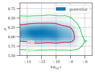
Figure 10: Posterior distribution of $(\epsilon,\mu)$ parameters for the MSP population with $\ell_{\text{max}}=5$ using the HLV data.

IX future prospects

Given the current sensitivity of ground-based GW detectors, it is challenging to detect any kind of anisotropic SGWB at this point. Rather, it would be of our greater interest to assess the future prospect of detectability or constraints on model parameters using projected sensitivity of current and next-generation detectors. Here, we present the results of simulated analyses using three different baseline configurations as follows:

• the two LIGO, Virgo and KAGRA detectors with their design sensitivities (HLVK design)

• the two LIGO, Virgo, KAGRA and LIGO-India detectors with the A+ sensitivities (HLVKI A+)

• the two LIGO, Virgo, KAGRA and LIGO-India detectors with the A+ sensitivities as well as Cosmic Explorer (HLVKI+CE)

For each 1 sidereal-day dataset, we conduct two analyses with and without a background signal injected. The injected signal model follows the PL $\bar{H}(f)$ and the Galactic plane $\bar{\cal P}_{\ell m}$ model with the same injected parameters $(\epsilon,\alpha)=(2.608\times 10^{-6},3.857)$ as the one in Sec. V.2 and $\ell_{\text{max}}=7$. This injected signal is recovered with the consistent signal model using the same prior distribution as the injection recovery in Fig. 2, and the 2D posterior result for each dataset is shown in Fig. 11, where the injected values are indicated by the red star. The inner and outer contours represent the $65\%$ and $95\%$ confidence region, respectively.

We find the BF of these signal recoveries to be roughly $10^{5},10^{7},10^{12}$ for the injection in the “HLVK design”,“HLVKI A+”,“HLVKI+CE” datasets, respectively. Regarding the uncertainty in parameter inference, the “HLVK design” network improves it by a factor of 2 compared to that shown in Fig. 2, where the network configuration contains only the two LIGO detectors with the same design sensitivity. Furthermore, the uncertainties for “HLVKI A+” (“HLVKI+CE”) network decrease by another one (three) order(s) of magnitudes. Nevertheless, we should note that these future configurations would be so sensitive that the energy spectrum of a background signal itself might act as another source of noise background. Since the current formalism does not account for the effect of this additional noise, we regard the results shown in Fig. 11 as highly optimistic and leave more thorough analysis without the weak-signal assumption as future work.

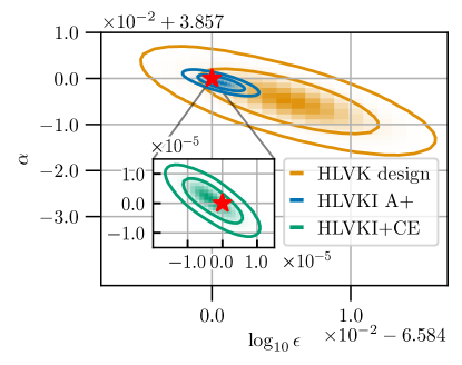
Figure 11: Posterior distribution for the same detected injection as Fig. 2. The inner and outer contour for each distribution represent 1$\sigma~{}(68\%)$ and 2$\sigma~{}(95\%)$ credible region.

On the other hand, the results for the noninjection analysis are presented in Fig. 12. For each dataset, we use the same prior distribution as the signal recovery in Fig. 3 and draw a contour that represents the $95\%$ confidence region. While all the datasets yield similar constraints for $\alpha$, the upper limit of $\epsilon$ becomes more stringent by a half (three) order(s) of magnitudes for “HLVKI A+” (“HLVKI+CE”) compared to Fig. 3. This demonstrates how significantly the constraints on the background amplitudes would improve for next generations of GW detector networks.

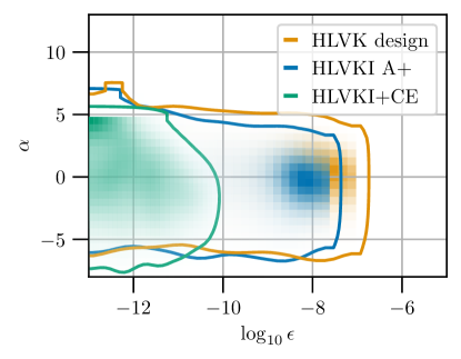
Figure 12: Posterior distribution for dataset using each future detector network without any injection. The contours for each distribution represent 2$\sigma~{}(95\%)$ credible region for parameter constraints.

X Conclusion

In this paper, we introduced a parameter estimation formalism targeted for an anisotropic SGWB from extended sources. Following the Bayesian framework, this formalism provides the posterior distribution of model parameters for a given anisotropy model $\bar{\cal P}_{\ell m}$, which can be seen as an extension from the Bayesian parameter estimation for isotropic SGWB with higher spatial modes in a signal model. We also developed data simulation and signal injection tools on the spherical-harmonics bases, which allow us to conduct injection studies to assess statistical consistency of posterior results. The study we conducted using the Galactic plane model showed validity of the posterior results given by our analysis [see Fig. 4].

Also, this formalism brings additional novelties such as a model selection between different $\bar{\cal P}_{\ell m}$ or $\bar{H}(f)$ models and a systematic method to optimize $\ell_{\text{max}}$ value for given $\bar{\cal P}_{\ell m}$, both of which make use of the comparison of the BF. In particular, we explored the parameter region where our pipeline can distinguish two different signal models in various cases, e.g., PL and BPL $\bar{H}(f)$ models, or isotropic and the Galactic plane $\bar{\cal P}_{\ell m}$ models. We noted that the structure of the distinguishable parameter region was consistent with our expectation. [see Figs. (6,7)] Regarding the $\ell_{\text{max}}$ optimization, we found that, throughout injected signal amplitudes that are loud enough, the recovery $\ell_{\text{max}}$ maximizes the BF when it was matched with the $\ell_{\text{max}}$ value used for the signal injection. [see Fig. 8]

Finally, we conducted an analysis to search for the MSP population using the real data from the LVK’s O3. We didn’t have any strong evidence of such a SGWB signal in the data and placed the constraints on the amplitude $\epsilon\leq 2.7\times 10^{-8}$ (95% upper limit). We also simulated analyses using the projected sensitivities of future GW detector networks. The analyses demonstrated that the upgrade to the A+ sensitivity or the addition of CE improves the precision of parameter estimation by one or three orders of magnitudes, respectively. We also assessed the constraints potentially placed on the same parameters and obtain similar degrees of the improvements. This indicates promising insights into the search for anisotropic SGWBs in the future observations.

Appendix A POTENTIAL BIAS IN ISOTROPIC ANALYSIS

In the injection studies shown in Sec. V, we adopt the same $\ell_{\text{max}}$ for both the injection and its recovery, and verify the statistical consistency in the parameter inference. In reality, however, we do not know the spatial scale of a background signal in nature a priori, and it is possible that one does not recover the signal with a consistent $\ell_{\text{max}}$ value. Especially, isotropic SGWB searches (i.e. $\ell_{\text{max}}=0$ for recovery) always ignore any higher spherical-harmonics mode and hence, for future configurations with greater sensitivities, it is crucial to investigate the potential impact of the $\ell_{\text{max}}$ inconsistency to the parameter inference. Here, we describe the results of an injection study similar to what is shown in Sec. V.3.

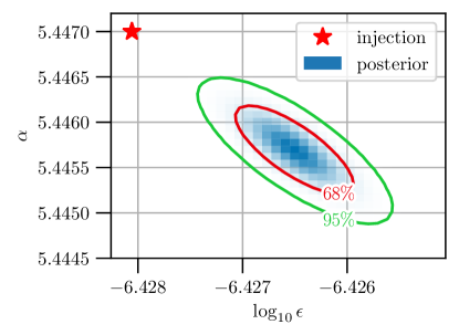
Figure 13: Posterior distribution for one of the detected injections that indicate a strong bias in the signal recovery. The injected values are $(\log_{10}\epsilon,\alpha)=(-6.428,5.447)$ and the BF is $\sim 5.6\times 10^{7}$.

We use the same dataset with injections produced from the same signal model and parameter values of ($\epsilon,\alpha$) as used for Sec. V.3, setting $\ell_{\text{max}}=3$. Each of these injections is recovered with the consistent signal model as well as the same prior distribution except $\ell_{\text{max}}=0$ to simulate an isotropic SGWB analysis. Figure 13 exemplifies a typical bias of the parameter inference seen in one of the 2D posterior results. Given the relatively large BF ($\sim 6\times 10^{7}$) found for the injection shown in Fig. 13, we note that this bias tends to be more noticeable for louder injections.

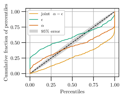
Figure 14: Probability-probability plot for 500 of the injection recoveries using the recovery $\ell_{\text{max}}=0$. Different colors indicate each method of computing the percentile by either 1D marginalized or 2D joint distribution. The gray region is the 95% confidence region expected from the Poisson fluctuation.

In order to assess a statistical picture, a P-P plot for these injection recoveries is produced and shown in Fig. 14. Apart from the percentile computed for the 2D $\alpha-\epsilon$ posterior as explained in Sec. V.3, we also plot percentiles evaluated for each of the 1D marginalized posteriors. Unlike the $\ell_{\text{max}}=3$ case in Fig. 4, all three curves clearly deviate from the $95\%$ error region. Therefore, this result suggests that the parameter inference is systematically biased when the recovery $\ell_{\text{max}}$ is not consistent with the one characterizing a real signal, which will be particularly impactful in the conventional isotropic analysis in the future. Aiming to avoid this bias, we discuss a quantitative approach to optimize the recovery $\ell_{\text{max}}$ in Sec. VII.

References

- Abbott et al. [2016] B. P. Abbott et al. (LIGO Scientific Collaboration and Virgo Collaboration), Phys. Rev. Lett. . 116, 061102 (2016).
- Abbott et al. [2019a] B. Abbott, R. Abbott, T. Abbott, S. Abraham, F. Acernese, K. Ackley, C. Adams, R. Adhikari, V. Adya, C. Affeldt, et al., Physical Review X 9, 031040 (2019a).
- Abbott et al. [2020] R. Abbott et al. (LIGO Scientific Collaboration, and VIRGO Collaboration), (2020), arXiv:2010.14527 [gr-qc] .
- The LIGO Scientific Collaboration et al. [2021a] The LIGO Scientific Collaboration, The Virgo Collaboration, R. Abbott, et al., “Gwtc-2.1: Deep extended catalog of compact binary coalescences observed by ligo and virgo during the first half of the third observing run,” (2021a).
- The LIGO Scientific Collaboration et al. [2021b] The LIGO Scientific Collaboration, The Virgo Collaboration, The KAGRA Collaboration, R. Abbott, et al., “Gwtc-3: Compact binary coalescences observed by ligo and virgo during the second part of the third observing run,” (2021b).
- Aasi et al. [2015] J. Aasi et al. (LIGO Scientific Collaboration), Class. Quant. Grav. 32, 074001 (2015), arXiv:1411.4547 [gr-qc] .
- Acernese et al. [2015] F. Acernese et al. (Virgo Collaboration), Class. Quant. Grav. 32, 024001 (2015), arXiv:1408.3978 [gr-qc] .
- Akutsu et al. [2020] T. Akutsu et al., “Overview of kagra: Detector design and construction history,” (2020).
- Saleem et al. [2021] M. Saleem, J. Rana, V. Gayathri, A. Vijaykumar, S. Goyal, S. Sachdev, J. Suresh, S. Sudhagar, A. Mukherjee, G. Gaur, B. Sathyaprakash, A. Pai, R. X. Adhikari, P. Ajith, and S. Bose, Classical and Quantum Gravity 39, 025004 (2021).
- Punturo et al. [2010a] M. Punturo et al., Classical and Quantum Gravity 27, 194002 (2010a).
- others [2011] S. H. others, Classical and Quantum Gravity 28, 094013 (2011).
- Punturo et al. [2010b] M. Punturo et al., Class. Quantum Gravity 27, 084007 (2010b).
- Maggiore et al. [2020] M. Maggiore, C. V. D. Broeck, N. Bartolo, E. Belgacem, D. Bertacca, M. A. Bizouard, M. Branchesi, S. Clesse, S. Foffa, J. García-Bellido, S. Grimm, J. Harms, T. Hinderer, S. Matarrese, C. Palomba, M. Peloso, A. Ricciardone, and M. Sakellariadou, Journal of Cosmology and Astroparticle Physics 2020, 050 (2020).
- Abbott et al. [2017] B. P. Abbott et al., Classical and Quantum Gravity 34, 044001 (2017).
- Renzini et al. [2022] A. I. Renzini, B. Goncharov, A. C. Jenkins, and P. M. Meyers, “Stochastic gravitational-wave backgrounds: Current detection efforts and future prospects,” (2022).
- Regimbau and Mandic [2008] T. Regimbau and V. Mandic, Class. Quantum Gravity 25, 184018 (2008).
- Regimbau [2022] T. Regimbau, Symmetry 14, 270 (2022).
- Banagiri et al. [2020] S. Banagiri, V. Mandic, C. Scarlata, and K. Z. Yang, Phys. Rev. D 102, 063007 (2020), arXiv:2006.00633 [astro-ph.CO] .
- Payne et al. [2020] E. Payne, S. Banagiri, P. Lasky, and E. Thrane, Phys. Rev. D 102, 102004 (2020), arXiv:2006.11957 [astro-ph.CO] .
- Stiskalek et al. [2020] R. Stiskalek, J. Veitch, and C. Messenger, (2020), 10.1093/mnras/staa3613, arXiv:2003.02919 [astro-ph.HE] .
- Marassi et al. [2009] S. Marassi, R. Schneider, and V. Ferrari, Mon. Not. R. Ast. Soc. 398, 293 (2009).
- Zhu et al. [2010] X.-J. Zhu, E. Howell, and D. Blair, Mon. Not. R. Ast. Soc. 409, L132 (2010).
- Buonanno et al. [2005] A. Buonanno, G. Sigl, G. G. Raffelt, H.-T. Janka, and E. Müller, Phys. Rev. D 72, 084001 (2005).
- Sandick et al. [2006] P. Sandick, K. A. Olive, F. Daigne, and E. Vangioni, Phys. Rev. D 73, 104024 (2006).
- Cavaglià and Modi [2020] M. Cavaglià and A. Modi, Universe 6 (2020), 10.3390/universe6070093.
- Brito et al. [2017a] R. Brito, S. Ghosh, E. Barausse, E. Berti, V. Cardoso, I. Dvorkin, A. Klein, and P. Pani, Phys. Rev. Lett. 119, 131101 (2017a), arXiv:1706.05097 [gr-qc] .
- Brito et al. [2017b] R. Brito, S. Ghosh, E. Barausse, E. Berti, V. Cardoso, I. Dvorkin, A. Klein, and P. Pani, Phys. Rev. D96, 064050 (2017b), arXiv:1706.06311 [gr-qc] .
- Fan and Chen [2018] X.-L. Fan and Y.-B. Chen, Phys. Rev. D98, 044020 (2018), arXiv:1712.00784 [gr-qc] .
- Tsukada et al. [2019] L. Tsukada, T. Callister, A. Matas, and P. Meyers, Phys. Rev. D99, 103015 (2019), arXiv:1812.09622 [astro-ph.HE] .
- Palomba et al. [2019] C. Palomba, S. D’Antonio, P. Astone, S. Frasca, G. Intini, I. La Rosa, P. Leaci, S. Mastrogiovanni, A. L. Miller, F. Muciaccia, et al., Physical Review Letters 123, 171101 (2019).
- Sun et al. [2019] L. Sun, R. Brito, and M. Isi, arXiv preprint arXiv:1909.11267 (2019).
- Bar-Kana [1994] R. Bar-Kana, Phys. Rev. D 50, 1157 (1994).
- Starobinskiǐ [1979] A. A. Starobinskiǐ, Soviet Journal of Experimental and Theoretical Physics Letters 30, 682 (1979).
- Easther et al. [2007] R. Easther, J. T. Giblin, Jr., and E. A. Lim, Physical Review Letters 99, 221301 (2007).
- Barnaby et al. [2012] N. Barnaby, E. Pajer, and M. Peloso, Phys. Rev. D 85, 023525 (2012).
- Cook and Sorbo [2012] J. L. Cook and L. Sorbo, Phys. Rev. D 85, 023534 (2012).
- Lopez and Freese [2015] A. Lopez and K. Freese, JCAP 1501, 037 (2015), arXiv:1305.5855 [astro-ph.HE] .
- Turner [1997] M. S. Turner, Phys. Rev. D 55, 435 (1997).
- Easther and Lim [2006] R. Easther and E. A. Lim, JCAP 4, 010 (2006).
- Crowder et al. [2013] S. G. Crowder, R. Namba, V. Mandic, S. Mukohyama, and M. Peloso, Physics Letters B 726, 66 (2013), arXiv:1212.4165 .
- Von Harling et al. [2020] B. Von Harling, A. Pomarol, O. Pujolàs, and F. Rompineve, JHEP 04, 195 (2020), arXiv:1912.07587 [hep-ph] .
- Dev and Mazumdar [2016] P. S. B. Dev and A. Mazumdar, Phys. Rev. D 93, 104001 (2016), arXiv:1602.04203 [hep-ph] .
- Marzola et al. [2017] L. Marzola, A. Racioppi, and V. Vaskonen, Eur. Phys. J. C 77, 484 (2017), arXiv:1704.01034 [hep-ph] .
- Mandic et al. [2016] V. Mandic, S. Bird, and I. Cholis, Phys. Rev. Lett. 117, 201102 (2016).
- Sasaki et al. [2016] M. Sasaki, T. Suyama, T. Tanaka, and S. Yokoyama, Phys. Rev. Lett. 117, 061101 (2016).
- Wang et al. [2018] S. Wang, Y.-F. Wang, Q.-G. Huang, and T. G. F. Li, Phys. Rev. Lett. 120, 191102 (2018), arXiv:1610.08725 [astro-ph.CO] .
- Miller et al. [2020] A. L. Miller, S. Clesse, F. De Lillo, G. Bruno, A. Depasse, and A. Tanasijczuk, (2020), arXiv:2012.12983 [astro-ph.HE] .
- Contaldi [2017] C. R. Contaldi, Physics Letters B 771, 9 (2017), arXiv:1609.08168 .
- Jenkins et al. [2019a] A. C. Jenkins, O. Richard, M. Sakellariadou, and D. Wysocki, Physical Review Letters 122, 111101 (2019a).
- Jenkins and Sakellariadou [2019] A. C. Jenkins and M. Sakellariadou, Phys. Rev. D 100, 063508 (2019), arXiv:1902.07719 [astro-ph.CO] .
- Jenkins et al. [2019b] A. C. Jenkins, J. D. Romano, and M. Sakellariadou, Phys. Rev. D 100, 083501 (2019b), arXiv:1907.06642 [astro-ph.CO] .
- Bertacca et al. [2020] D. Bertacca, A. Ricciardone, N. Bellomo, A. C. Jenkins, S. Matarrese, A. Raccanelli, T. Regimbau, and M. Sakellariadou, Phys. Rev. D 101, 103513 (2020), arXiv:1909.11627 [astro-ph.CO] .
- Cusin et al. [2017] G. Cusin, C. Pitrou, and J.-P. Uzan, Phys. Rev. D 96, 103019 (2017), arXiv:1704.06184 .
- Cusin et al. [2018a] G. Cusin, C. Pitrou, and J.-P. Uzan, Phys. Rev. D97, 123527 (2018a), arXiv:1711.11345 [astro-ph.CO] .
- Cusin et al. [2018b] G. Cusin, I. Dvorkin, C. Pitrou, and J.-P. Uzan, Phys. Rev. Lett. 120, 231101 (2018b), arXiv:1803.03236 [astro-ph.CO] .
- Cusin et al. [2019] G. Cusin, I. Dvorkin, C. Pitrou, and J.-P. Uzan, Phys. Rev. D 100, 063004 (2019), arXiv:1904.07797 [astro-ph.CO] .
- Pitrou et al. [2020] C. Pitrou, G. Cusin, and J.-P. Uzan, Phys. Rev. D 101, 081301 (2020), arXiv:1910.04645 [astro-ph.CO] .
- Cañas Herrera et al. [2020] G. Cañas Herrera, O. Contigiani, and V. Vardanyan, Phys. Rev. D 102, 043513 (2020), arXiv:1910.08353 [astro-ph.CO] .
- Geller et al. [2018] M. Geller, A. Hook, R. Sundrum, and Y. Tsai, Phys. Rev. Lett. 121, 201303 (2018), arXiv:1803.10780 [hep-ph] .
- Abbott et al. [2009] B. P. Abbott et al. (LIGO Scientific Collaboration and Virgo Collaboration), Nature 460, 990 (2009).
- Abbott et al. [2017a] B. P. Abbott et al. (LIGO Scientific Collaboration and Virgo Collaboration), Physical Review Letters 118, 121101 (2017a), arXiv:1612.02029 [gr-qc] .
- Abbott et al. [2019b] B. Abbott, R. Abbott, T. Abbott, S. Abraham, F. Acernese, K. Ackley, C. Adams, V. Adya, C. Affeldt, M. Agathos, and et al., Physical Review D 100 (2019b), 10.1103/physrevd.100.061101.
- Abbott et al. [2021a] R. Abbott et al., Physical Review D 104 (2021a), 10.1103/physrevd.104.022004.
- Abadie et al. [2011] J. Abadie et al. (LIGO Scientific Collaboration and Virgo Collaboration), Phys. Rev. Lett. 107, 271102 (2011).
- Abbott et al. [2017b] B. P. Abbott et al. (LIGO Scientific Collaboration and Virgo Collaboration), Physical Review Letters 118, 121102 (2017b), arXiv:1612.02030 [gr-qc] .
- Abbott et al. [2019c] B. Abbott, R. Abbott, T. Abbott, S. Abraham, F. Acernese, K. Ackley, C. Adams, R. Adhikari, V. Adya, C. Affeldt, et al., Physical Review D 100, 062001 (2019c).
- Abbott et al. [2021b] R. Abbott et al. (LIGO Scientific Collaboration, Virgo Collaboration, and KAGRA Collaboration), Phys. Rev. D 104, 022005 (2021b).
- asa [2022] Physical Review D 105 (2022), 10.1103/PhysRevD.105.122001.
- Ballmer [2006] S. W. Ballmer, Class. Quantum Gravity 23, S179 (2006).
- Ballmer [2006] S. Ballmer, LIGO interferometer operating at design sensitivity with application to gravitational radiometry, Ph.D. thesis, Massachusetts Institute of Technology (2006).
- Mitra et al. [2008] S. Mitra, S. Dhurandhar, T. Souradeep, A. Lazzarini, V. Mandic, S. Bose, and S. Ballmer, Phys. Rev. D 77, 042002 (2008).
- Thrane et al. [2009] E. Thrane, S. Ballmer, J. D. Romano, S. Mitra, D. Talukder, S. Bose, and V. Mandic, Phys. Rev. D 80, 122002 (2009).
- Agarwal [2022] D. Agarwal, Physical Review D 106 (2022), 10.1103/PhysRevD.106.043019.
- Chung et al. [2022] A. K.-W. Chung, A. C. Jenkins, J. D. Romano, and M. Sakellariadou, “Targeted search for the kinematic dipole of the gravitational-wave background,” (2022).
- Mandic [2012] V. Mandic, Physical Review Letters 109 (2012), 10.1103/PhysRevLett.109.171102.
- Meyers et al. [2020] P. M. Meyers, K. Martinovic, N. Christensen, and M. Sakellariadou, Physical Review D 102 (2020), 10.1103/physrevd.102.102005.
- Allen and Romano [1999] B. Allen and J. D. Romano, Phys. Rev. D 59, 102001 (1999).
- Romano and Cornish [2017] J. D. Romano and N. J. Cornish, Living reviews in relativity 20, 2 (2017).
- Allen and Ottewill [1997] B. Allen and A. C. Ottewill, Phys. Rev. D 56, 545 (1997).
- Sesana et al. [2008] A. Sesana, A. Vecchio, and C. N. Colacino, Monthly Notices of the Royal Astronomical Society 390, 192 (2008).
- Veitch et al. [2015] J. Veitch, V. Raymond, B. Farr, et al., Phys. Rev. D 91, 042003 (2015), arXiv:1409.7215 [gr-qc] .
- Ashton et al. [2019] G. Ashton et al., Astrophys. J. Suppl. 241, 27 (2019), arXiv:1811.02042 [astro-ph.IM] .
- Romero-Shaw et al. [2020] I. M. Romero-Shaw et al., Mon. Not. Roy. Astron. Soc. 499, 3295 (2020), arXiv:2006.00714 [astro-ph.IM] .
- Flanagan [1993] E. E. Flanagan, Phys. Rev. D 48, 2389 (1993).
- Speagle [2020] J. S. Speagle, Monthly Notices of the Royal Astronomical Society 493, 3132 (2020), arXiv:1904.02180 [astro-ph.IM] .
- Abbott et al. [2018] B. Abbott et al. (KAGRA Collabration, LIGO Scientific Collaboration, and VIRGO Collaboration), Living Rev. Rel. 21, 3 (2018), arXiv:1304.0670 [gr-qc] .
- [87] https://dcc.ligo.org/LIGO T2000012/public, “Noise curves used for simulations in the update of the observing scenarios paper,” .
- Gorski et al. [2005] K. M. Gorski, E. Hivon, A. J. Banday, B. D. Wandelt, F. K. Hansen, M. Reinecke, and M. Bartelman, Astrophys. J. 622, 759 (2005), arXiv:astro-ph/0409513 [astro-ph] .
- Kass and Raftery [1995] R. E. Kass and A. E. Raftery, Journal of the American Statistical Association 90, 773 (1995).
- Floden et al. [2022] E. Floden, V. Mandic, A. Matas, and L. Tsukada, “Angular resolution of the search for anisotropic stochastic gravitational-wave background with terrestrial gravitational-wave detectors,” (2022).
- LIGO Scientific Collaboration [2022] V. C. LIGO Scientific Collaboration, “Folded data for first three observing runs of advanced ligo and advanced virgo,” (2022).
- Ain et al. [2015] A. Ain, P. Dalvi, and S. Mitra, Phys. Rev. D 92, 022003 (2015).
- Ain et al. [2018] A. Ain, J. Suresh, and S. Mitra, Phys. Rev. D 98, 024001 (2018), arXiv:1803.08285 [gr-qc] .
- Suresh et al. [2021] J. Suresh, A. Ain, and S. Mitra, Phys. Rev. D 103, 083024 (2021).
- De Lillo et al. [2022] F. De Lillo, J. Suresh, and A. L. Miller, Monthly Notices of the Royal Astronomical Society 513, 1105 (2022), https://academic.oup.com/mnras/article-pdf/513/1/1105/43471376/stac984.pdf .
- Lorimer et al. [2015] D. R. Lorimer, P. Esposito, R. N. Manchester, A. Possenti, A. G. Lyne, M. A. McLaughlin, M. Kramer, G. Hobbs, I. H. Stairs, M. Burgay, R. P. Eatough, M. J. Keith, A. J. Faulkner, N. D'Amico, F. Camilo, A. Corongiu, and F. Crawford, Monthly Notices of the Royal Astronomical Society 450, 2185 (2015).