Polynomial Almost-Complex Curves in $\mathbb{S}^{2,4}$

Abstract

For solutions of the $\mathfrak{g}_{2}$ affine Toda field equations in $\mathbb{C}$ with respect to polynomial $q\in H^{0}(\mathcal{K}_{\mathbb{C}}^{6})$, we study the associated almost-complex curves $\nu_{q}:\mathbb{C}\rightarrow\mathbb{S}^{2,4}$. The asymptotic boundary $\Delta:=\partial_{\infty}(\nu_{q})$ of $\nu_{q}$ is found to be a polygon in $\mathsf{Ein}^{2,3}$ with $\deg q+6$ vertices. The polygon $\Delta$ satisfies an annihilator property, which is related to a $\mathsf{G}_{2}^{\prime}$-invariant discrete metric $d_{3}:\mathsf{Ein}^{2,3}\times\mathsf{Ein}^{2,3}\rightarrow\{0,1,2,3\}$ on $\mathsf{Ein}^{2,3}$. In fact, we show $\mathsf{G}_{2}^{\prime}=\mathsf{Isom}(d_{3})\cap\mathsf{Diff}(\mathsf{Ein}^{2,3})$. The asymptotic boundary defines a map $\alpha:\mathsf{MS}_{k}\rightarrow\mathsf{MP}_{k+6}$ between the equidimensional moduli spaces of holomorphic polynomial sextic differentials of degree $k$ and of annihilator polygons with $k+6$ vertices and is conjectured to be a homeomorphism onto its image. We also discuss the relationship between $\nu_{q}$ the minimal surface $f_{q}:\mathbb{C}\rightarrow\mathsf{G}_{2}^{\prime}/K$, relating these maps to a mutual harmonic lift to $\mathsf{G}_{2}^{\prime}/T$, realized geometrically. Before beginning the geometry, we prove the existence and uniqueness of a complete (real) solution to the $\mathfrak{g}_{2}$ affine Toda field equations in $\mathbb{C}$ associated to polynomial $q\in H^{0}(\mathcal{K}_{\mathbb{C}}^{6})$.

1 Introduction

We first provide a brief overview of the main objects and results. Almost complex curves $\phi:\Sigma\rightarrow(\mathbb{S}^{6},J_{\mathbb{S}^{6}})$ from a Riemann surface $\Sigma$ are now well-studied, though the same is not true for almost-complex curves in $(\hat{\mathbb{S}}^{2,4},J_{\hat{\mathbb{S}}^{2,4}})$. Let $\mathsf{G}_{2}^{\prime}$ denote the split real form of the complex exceptional Lie group $\mathsf{G}_{2}$. In 2010, Baraglia constructed $\rho$-equivariant almost-complex curves $\nu:\widetilde{\Sigma}\rightarrow\hat{\mathbb{S}}^{2,4}$ associated to representations $\rho:\pi_{1}\Sigma\rightarrow\mathsf{G}_{2}^{\prime}$ in the Hitchin component. However, Baraglia does not describe the geometry of the image of such curves, and this geometry has remained unexplored. This paper studies the asymptotic geometry of almost-complex curves $\nu_{q}:\mathbb{C}\rightarrow\hat{\mathbb{S}}^{2,4}$, now in the planar setting.

The curves $\nu_{q}$ are associated to a holomorphic sextic differential $q\in H^{0}(\mathcal{K}^{6}_{\mathbb{C}})$ by solving a $2\times 2$ coupled system of PDE called the $\mathfrak{g}_{2}$ affine Toda (field) equations (with appropriate reality conditions). First, we prove the existence and uniqueness of complete solutions to these equations when $q$ is a polynomial (c.f. Theorem A).

We next show that the asymptotic boundary $\Delta=\partial_{\infty}(\,\nu_{q})$ a polynomial almost-complex curve $\nu_{q}:\mathbb{C}\rightarrow\hat{\mathbb{S}}^{2,4}$ is a polygon in the space $\mathsf{Ein}^{2,3}$, the frontier of $\mathbb{S}^{2,4}$ in $\mathbb{P}(\mathbb{R}^{3,4})$. The polygon $\Delta$ satisfies a condition we call the annihilator property (c.f. Theorem B, Theorem B’). We then give descriptions of $\mathsf{G}_{2}^{\prime}$ as the subgroup of the diffeomorphism group $\mathsf{Diff}(\mathsf{Ein}^{2,3})$ preserving various forms of annihilators (c.f. Theorem C). Moreover, Theorem B allows us to define a map $\alpha:\mathsf{TS}_{k}\rightarrow\mathsf{TP}_{k+6}$ between a vector space of holomorphic polynomial sextic differentials of degree $k$ in $\mathbb{C}$ and a moduli of space of marked annihilator polygons with $k+6$ vertices. The space $\mathsf{TS}_{k}\cong_{\mathbf{Top}}\mathbb{R}^{2(k-1)}$ is a cell of real dimension $2(k-1)$. On the other hand, $\mathsf{TP}_{k+6}$ consists of a disjoint union of cells of dimension $2(k-1)$, along with lower-dimensional strata [24]. Hence, this dimension count invites the question of whether the map $\alpha$ is injective and moreover whether $\alpha$ furnishes a homeomorphism with a component of $\mathsf{TP}_{k+6}$.

Along the way, we discuss the geometric relationship between the minimal surface $f_{q}:\mathbb{C}\rightarrow\mathsf{G}_{2}^{\prime}/K$ in the symmetric space associated to $q$ and the almost-complex complex curve $\nu_{q}$. Each map carries equivalent data, as they each lift to a harmonic map in $\mathsf{G}_{2}^{\prime}/T$, where $T<K$ is a maximal torus.

1.1 Background

Harmonic maps from a Riemann surface $\Sigma$ into $\mathbb{S}^{n},\mathbb{R}\mathbb{P}^{n},\mathbb{C}\mathbb{P}^{n}$ are now classical [9, 22]. Among such target spaces, $\mathbb{S}^{6}$ is exceptional since it carries a canonical almost-complex structure $J_{\mathbb{S}^{6}}$. Any almost-complex curve $\phi:\Sigma\rightarrow(\mathbb{S}^{6},J_{\mathbb{S}^{6}})$ is weakly conformal, harmonic, and still harmonic when regarded as a map into $\mathbb{R}\mathbb{P}^{6}$ or $\mathbb{C}\mathbb{P}^{6}$. Some rich geometry has been discovered by studying these almost-complex curves [7, 8, 13, 25, 31, 62].

Let us now relate $(\mathbb{S}^{6},J_{\mathbb{S}^{6}})$ to the present setting. The almost-complex structure $J_{\mathbb{S}^{6}}$ is invariant under the compact, real form $\mathsf{G}_{2}^{c}$ of $\mathsf{G}_{2}$. We study instead the almost-complex manifold $(\hat{\mathbb{S}}^{2,4},J_{\hat{\mathbb{S}}^{2,4}})$, now invariant under the split real form $\mathsf{G}_{2}^{\prime}$. These Lie groups can be realized as $\mathsf{G}_{2}^{\prime}:=\mathsf{Aut}_{\mathbb{R}-\mathbf{alg}}(\mathbb{O}^{\prime})$ and $\mathsf{G}_{2}^{c}:=\mathsf{Aut}_{\mathbb{R}-\mathbf{alg}}(\mathbb{O})$, where $\mathbb{O}$ and $\mathbb{O}^{\prime}$ are the octonions and split octonions, respectively. Both $\mathbb{O}$ and $\mathbb{O}^{\prime}$ are real algebras (with unit) over 8-dimensional vector spaces and are endowed with various algebraic structures $q,\odot,\times$, all of which are invariant under the relevant real form of $\mathsf{G}_{2}$; see Section 2.1 for details. These algebraic structures on $\mathbb{O}$ and $\mathbb{O}^{\prime}$ lead to the almost-complex structures $J_{\hat{\mathbb{S}}^{2,4}}$ and $J_{\mathbb{S}^{6}}$. For brevity, we describe $\mathbb{O}$ first and note the relevant differences for $\mathbb{O}^{\prime}$. The octonions are equipped with a Euclidean inner product $q_{\mathbb{O}}$. Taking the imaginary octonions by orthogonally splitting $\mathbb{O}=\mathbb{R}\{1_{\mathbb{O}}\}\oplus\mathsf{Im}\,\mathbb{O}$, the space $\mathsf{Im}\,\mathbb{O}$ comes equipped with a cross-product $\times_{\mathbb{O}}:\mathsf{Im}\,\mathbb{O}\times\mathsf{Im}\,\mathbb{O}\rightarrow\mathsf{Im}\,\mathbb{O}$ in the sense that $\times_{\mathbb{O}}$ is skew-symmetric, orthogonal (with respect to $q_{\mathbb{O}}$), and normalized by $q_{\mathbb{O}}(u\times_{\mathbb{O}}v)=q_{\mathbb{O}}(u)q_{\mathbb{O}}(v)-q_{\mathbb{O}}(u,v)^{2}$. Denote $Q_{+}(V,q):=\{x\in V\,|\,q(x)=+1\}$. Since $q_{\mathbb{O}}$ is Euclidean, identify $\mathbb{S}^{6}=Q_{+}(\mathsf{Im}\,\mathbb{O})$. Then $J_{\mathbb{S}^{6}}$ is defined at $x\in\mathbb{S}^{6}$ by identifying $T_{x}\mathbb{S}^{6}\cong[x^{\bot}\subset\mathsf{Im}\,\mathbb{O}]$ and setting $J_{x}(u)=x\times u$. On the other hand, $q_{\mathbb{O}^{\prime}}$ is of split signature (4,4). The pseudosphere $\hat{\mathbb{S}}^{2,4}:=Q_{+}(\mathsf{Im}\,\mathbb{O}^{\prime})$ obtains an almost-complex structure also via $J_{x}(u):=x\times_{\mathbb{O}^{\prime}}u$, now using the cross-product on $\mathsf{Im}\,\mathbb{O}^{\prime}$. We are naturally led to ask about almost-complex curves $\nu:\Sigma\rightarrow\hat{\mathbb{S}}^{2,4}$ from a Riemann surface $\Sigma$.

The same argument as in the $\mathbb{S}^{6}$ case tells us almost-complex curves $\nu:\Sigma\rightarrow\hat{\mathbb{S}}^{2,4}$ are weakly conformal, harmonic, and also harmonic when regarded as maps to $\mathbb{R}\mathbb{P}^{6}$ or $\mathbb{C}\mathbb{P}^{6}$. The pseudo-Riemannian metric $q_{\mathbb{O}^{\prime}}|_{\hat{\mathbb{S}}^{2,4}}$ is of signature $(2,4)$. Hence, the signature of the induced metric on $S=\text{im}\,\nu$ is not a priori prescribed. We study timelike almost-complex curves (negative-definite induced metric) with spacelike second fundamental form. Such almost-complex curves were first discussed by Baraglia in his PhD thesis [4]. However, Baraglia studied equivariant almost-complex curves $\nu_{q}:\widetilde{\Sigma}\rightarrow\hat{\mathbb{S}}^{2,4}$ associated to representations $\rho:\pi_{1}\Sigma\rightarrow\mathsf{G}_{2}^{\prime}$; these almost-complex curves are associated to a holomorphic sextic differential $q\in H^{0}(K_{\Sigma}^{6})$ by solving a $2\times 2$ coupled elliptic system of PDE called the $\mathfrak{g}_{2}$ affine Toda (field) equations. Instead, we focus on almost-complex curves $\nu_{q}:\mathbb{C}\rightarrow\hat{\mathbb{S}}^{2,4}$ associated to these equations for polynomial $q\in H^{0}(\mathcal{K}^{6}_{\mathbb{C}})$, in the planar (i.e., non-compact) setting. We study the asymptotic geometry of such curves.

1.2 Main Results

We now describe the main results of the paper. As noted, we study planar almost-complex curves $\nu_{q}:\mathbb{C}\rightarrow\hat{\mathbb{S}}^{2,4}$ associated to holomorphic sextic differential $q\in H^{0}(\mathcal{K}_{\mathbb{C}}^{6})$ that are polynomial, i.e., $q=\tilde{q}\,dz^{6}$ for $\tilde{q}$ a holomorphic polynomial. To furnish such curves, we must solve the $\mathfrak{g}_{2}$ affine Toda equations associated to $q$ on $\mathbb{C}$. To this end, we prove:

Theorem A: Let $q\in H^{0}(\mathcal{K}_{\mathbb{C}}^{6})$ be a holomorphic polynomial sextic differential. Then there exists a unique complete, real solution to the $\mathfrak{g}_{2}$ affine toda equations for $q$ on the complex plane.

The definition of complete can be found in definition 4.1. Given polynomial $q\in H^{0}(\mathcal{K}_{\mathbb{C}}^{6})$, the unique aforementioned complete solution $\boldsymbol{u}=(u_{1},u_{2})$ to the affine Toda equations provides a unique almost-complex curve $\nu=\nu_{q}:\mathbb{C}\rightarrow\hat{\mathbb{S}}^{2,4}$, up to global $\mathsf{G}_{2}^{\prime}$ isometry. We show that one recovers $q$ from $\nu_{q}$, up to an explicit constant $C$, by $q=C(\nu_{z}\times\nu_{zz})\cdot\nu_{zzz}$. We embed the surface in projective space via $\overline{\nu}:\mathbb{C}\rightarrow\mathbb{S}^{2,4}\hookrightarrow\mathbb{P}\mathsf{Im}\,\mathbb{O}^{\prime}\cong\mathbb{P}(\mathbb{R}^{3,4})$ and show that the asymptotic boundary of $\Sigma=\text{im}\overline{\nu}$ is a polygon $\Delta$ with $\deg q+6$ vertices. Here, we mean polygon in the geometric sense: a piecewise linear curve formed by the (projective) lines connecting adjacent vertices. The polygon $\Delta=(p_{i})_{i=1}^{N}$ is contained in $\mathsf{Ein}^{2,3}:=\{\,[x]\in\mathbb{P}\mathsf{Im}\,\mathbb{O}^{\prime}\;|\;q(x)=0\}$, the space of null lines in $\mathsf{Im}\,\mathbb{O}^{\prime}$. Defining $\mathsf{Ann}(u):=\{l\in\mathbb{P}(\mathsf{Im}\,\mathbb{O}^{\prime})\;|\;l\times_{\mathbb{O}^{\prime}}u=0\}$ as in [3], we find $\Delta$ satisfies the annihilator property: $\mathsf{Ann}(p_{i})=\mathbb{P}(\mathsf{span}_{\mathbb{R}}<p_{i-1},p_{i},p_{i+1}>)$. That is, linear combinations of $p_{i}$ and its neighbors are exactly all the lines in $\mathbb{P}(\mathsf{Im}\,\mathbb{O}^{\prime})$ which annihilate the given line $p_{i}$. To summarize, our second main result is as follows:

Theorem B: Let $q\in H^{0}(\mathcal{K}_{\mathbb{C}}^{6})$ be polynomial, $\nu_{q}:\mathbb{C}\rightarrow\mathbb{S}^{2,4}$ its associated almost-complex curve. Then the boundary at infinity $\Delta=\partial_{\infty}\nu_{q}\subset\mathsf{Ein}^{2,3}$ is an annihilator polygon with $\deg q+6$ vertices.

We now give two reformulations of Theorem B after discussing some structures on $\mathsf{Ein}^{2,3}$. First, as a corollary to the proof (Theorem 16 [3]) that the diagonal action of $\mathsf{G}_{2}^{\prime}$ on $\mathsf{Ein}^{2,3}\times\mathsf{Ein}^{2,3}$ has exactly 4 orbits, we show there is a $\mathsf{G}_{2}^{\prime}$-invariant discrete metric $d_{3}:\mathsf{Ein}^{2,3}\times\mathsf{Ein}^{2,3}\rightarrow\{0,1,2,3\}$ defined by labeling the orbit the pair comes from. $\mathsf{Ein}^{2,3}$ also carries a canonical (2,3,5) distribution $\mathscr{D}$, invariant under $\mathsf{G}_{2}^{\prime}$. That is, $\mathscr{D}$ is maximally non-integrable in the sense that $\mathscr{D}^{1}:=\mathscr{D}+[\mathscr{D},\mathscr{D}]$ is 3-dimensional and $\mathscr{D}^{2}:=\mathscr{D}^{1}+[\mathscr{D}^{1},\mathscr{D}^{1}]$ is 5-dimensional. In fact, $\mathfrak{g}_{2}^{\prime}$ was first described by Cartan as the space of infinitesimal symmetries of $(\mathsf{Ein}^{2,3},\mathscr{D})$ [1]. We refer the reader to [1] for further history of $\mathsf{G}_{2}$, however, we remark $\mathscr{D}$ was only later connected the annihilator as we have defined it (c.f. [55], Appendix C [10]). Both $\mathscr{D},d_{3}$ allow us to give reinterpretations of the annihilator condition.

Theorem B’: Let $(p_{i})_{i=1}^{n}=\Delta\subset\mathsf{Ein}^{2,3}$ be the boundary at infinity of a polynomial almost-complex curve. Ordering the vertices $(p_{i})_{i=1}^{n}$ cyclically,

• $d_{3}(p_{i},p_{i+j})=j$ for $j\in\{0,1,2,3\}$.

• Away from the vertices, $\Delta$ is an integral curve of the (2,3,5) distribution $\mathscr{D}$ on $\mathsf{Ein}^{2,3}$.

Define $d_{\mathsf{graph}}(p_{i},p_{j}):=\min\{i-j,i-(n-j)\}$ as the distance between vertices on $\Delta$ as a graph. Then Theorem B’ says $d_{3}(p_{i},p_{j})=d_{\mathsf{graph}}(p_{i},p_{j})$ for $|j-i|\leq 3$. We currently do not know whether $d_{3}(p_{i},p_{i+j})=3$ when $d_{\mathsf{graph}}(p_{i},p_{j})>3$.

We also prove new results relating $\mathsf{G}_{2}^{\prime}$ to annihilators in various formulations, as we now describe. Denote $\mathsf{Diff}(\mathsf{Ein}^{2,3})$ as the group of diffeomorphisms of $\mathsf{Ein}^{2,3}$. By (Theorem 12 [3]), $\mathsf{Ann}([u])\cong_{\mathbf{Diff}}\mathbb{R}\mathbb{P}^{2}$ is a 2-dimensional submanifold of $\mathsf{Ein}^{2,3}$ for $[u]\in\mathsf{Ein}^{2,3}$. We say $\varphi\in\mathsf{Diff}(\mathsf{Ein}^{2,3})$ preserves annihilator submanifolds when $\varphi(\mathsf{Ann}(x))=\mathsf{Ann}(\varphi(x))$ for $x\in\mathsf{Ein}^{2,3}$. We say $\varphi$ preserves annihilators infinitesimally when $\varphi^{*}\mathscr{D}=\mathscr{D}$. We have one final notion of annihilators. Namely, given $x,y\in\mathsf{Ein}^{2,3}$ such $d_{3}(\,x,y)=1$, or equivalently, $x\times y=0$, we form the projective line $\mathscr{L}_{x,y}:=\mathbb{P}\,(\mathsf{span}_{\mathbb{R}}<x,y>\,)\subset\mathsf{Ein}^{2,3}$, since $x\cdot y=0$. Then we say $\varphi$ preserves annihilator lines when $\varphi(\mathscr{L}_{x,y})=\mathscr{L}_{\varphi(x),\varphi(y)}$ for all $x,y\in\mathsf{Ein}^{2,3}$ with $d_{3}(x,y)=1$. We show that all of these annihilator conditions are equivalent. (Here, recall $\mathsf{G}_{2}^{\prime}:=\mathsf{Aut}_{\mathbb{R}-\mathbf{alg}}(\mathbb{O}^{\prime})$ so that $\psi\in\mathsf{G}_{2}^{\prime}$ induces a diffeomorphism of $\mathsf{Ein}^{2,3}$ that we denote $\psi|_{\mathsf{Ein}^{2,3}}$.)

Theorem C: Let $F:\mathsf{G}_{2}^{\prime}\rightarrow\mathsf{Diff}(\mathsf{Ein}^{2,3})$ denote the map $F(\psi)=\psi|_{\mathsf{Ein}^{2,3}}$. Then $F$ is injective and $\varphi\in\mathsf{Diff}(\mathsf{Ein}^{2,3})$ satisfies $\varphi\in\text{im}F$ if and only if

• [15, 55] $\varphi$ preserves annihilators infinitesimally.

• $\varphi$ preserves annihilator submanifolds.

• $\varphi\in\mathsf{Isom}(d_{3})$.

• $\varphi$ preserves annihilator lines.

Thus, the group $\mathsf{G}_{2}^{\prime}$ is fundamentally linked to annihilators.

We also discuss the relationship between the almost-complex curve $\nu:\mathbb{C}\rightarrow\hat{\mathbb{S}}^{2,4}$ and the harmonic map $f:\mathbb{C}\rightarrow\mathcal{S}_{\mathsf{G}_{2}^{\prime}}$ into the symmetric space $\mathcal{S}_{\mathsf{G}_{2}^{\prime}}=\mathsf{G}_{2}^{\prime}/K$, where $K<\mathsf{G}_{2}^{\prime}$ is a maximal compact subgroup. In particular, the commutativity of the diagram in Figure 2 is established. We explain some of the diagram now. By work of Baraglia, associated to a (real) solution to the $\mathfrak{g}_{2}$ affine Toda is a harmonic lift into $\mathsf{G}_{2}^{\prime}/T$ of the harmonic map into the symmetric space, where $T<K$ is a maximal torus. While Baraglia’s work is done for general split real forms of complex simple Lie groups, we attempt to explain this lift in as concrete and geometric fashion as possible in the $\mathsf{G}_{2}^{\prime}$ setting. To this end, we identify $\mathsf{G}_{2}^{\prime}/K\cong_{\mathbf{Diff}}\mathscr{X}:=\{P\in\mathsf{Gr}_{(3,0)}(\mathsf{Im}\,\mathbb{O}^{\prime})\;|\;P\times P=P\}$ and $\mathsf{G}_{2}^{\prime}/T$ as a space of certain block-decompositions $\mathscr{Y}$ of $\mathsf{Im}\,\mathbb{O}^{\prime}$. Using these geometric descriptions, we explain how an almost-complex curve $\nu$ admits a natural lift $G_{\nu}:\mathbb{C}\rightarrow\mathscr{Y}$. We also realize a “geometric” version of the harmonic map in the symmetric space as $f:\mathbb{C}\rightarrow\mathscr{X}$. We then clarify the naturality of these constructions. The affine Toda frame field $e^{\Omega}$ of the almost-complex curve defines a map $\hat{\mathcal{F}_{\nu}}:\mathbb{C}\rightarrow\mathsf{G}_{2}^{\prime}$ such that the projections $F_{K}:=\pi_{K}\circ\hat{\mathcal{F}_{\nu}}$ and $F_{T}:=\pi_{T}\circ\hat{\mathcal{F}_{\nu}}$ are harmonic, where $\pi_{T}:\mathsf{G}_{2}^{\prime}\rightarrow\mathsf{G}_{2}^{\prime}/T$ and $\pi_{K}:\mathsf{G}_{2}^{\prime}\rightarrow\mathsf{G}_{2}^{\prime}/K$. There is also a natural projection $\pi_{\mathbb{S}^{2,4}}:\mathscr{Y}\rightarrow\mathbb{S}^{2,4}$, where $\mathbb{S}^{2,4}=\{[x]\in\mathbb{P}\mathsf{Im}\,\mathbb{O}^{\prime}\;|\;q(x)>0\}$ is the projective model for the pseudosphere. The almost-complex curve $\nu$ is recovered (projectively) from the lift $G_{\nu}$ by $\nu=\pi_{\mathbb{S}^{2,4}}\circ G_{\nu}$. We show the equivalence of $F_{K},f$ and $F_{T},G_{\nu}$ in a large commutative diagram in Theorem 3.13. Identifying $\mathscr{Y}$ with $\mathsf{G}_{2}^{\prime}/T$, the map $G_{\nu}$ is harmonic and serves as a mutual lift of $\nu$ and $f$.

1.3 Related Work

Theorem A is closely related to recent work of Li & Mochizuki [48] on the existence and uniqueness of complete solutions to the $\mathfrak{sl}_{n}\mathbb{C}$ affine Toda equations on non-compact Riemann surfaces. Also related are the papers [6, 50] on solutions to Hitchin’s equations for cyclic wild Higgs bundles over $\mathbb{C}\mathbb{P}^{1}$. However, the $\mathfrak{g}_{2}$ affine Toda equations are not known to be linearly equivalent to the $\mathfrak{sl}_{n}\mathbb{C}$ affine Toda equations for any $n$. We remark further in Section 2.6.1 why there is no naive equivalence. Conversely, for a compact Riemann surface $\Sigma$ of genus $g>1$, Baraglia proved the existence and uniqueness of (real) solutions to the affine Toda field equations for any complex simple Lie algebra (Theorem 2 [5]).

Theorem B is a natural continuation of a line of work on maps $\phi:=\phi_{q}:\mathbb{C}\rightarrow X$ associated to polynomial holomorphic data $q\in H^{0}(\mathcal{K}_{\mathbb{C}}^{j})$ with polygonal boundary $\Delta:=\partial_{\infty}(\text{im}\,\phi_{q})$ [33, 21, 57, 58]. This theme begins in [33], where Han, Tam, Treibergs, and Wan show that any orientation-preserving harmonic map $\phi:\mathbb{C}\rightarrow H^{2},$ where $H^{2}$ is the hyperbolic plane in the disk model, that is a smooth embedding with polynomial Hopf differential $q_{2}$ has frontier an ideal polygon with $k+2$ vertices on $\partial_{\infty}H^{2}$. Even more closely related are the works [21, 57, 58], in which the geometric maps $\phi:\mathbb{C}\rightarrow X$ associated to polynomial holomorphic differential have asymptotic boundary a linear polygon and the map $\phi$ factors a harmonic map $f:\mathbb{C}\rightarrow\mathcal{S}_{G^{\mathbb{R}}}$ into the symmetric space $\mathcal{S}_{G^{\mathbb{R}}}$ of a split real rank 2 Lie group $G^{\mathbb{R}}$. For $G^{\mathbb{R}}=\mathsf{PSL}_{2}\mathbb{R}\times\mathsf{PSL}_{2}\mathbb{R}$, Tamburelli studied spacelike maximal surfaces in $\mathsf{AdS}_{3}$ associated to polynomial differential $q_{2}\in H^{0}(\mathcal{K}_{\mathbb{C}}^{2})$. For $G^{\mathbb{R}}=\mathsf{SL}_{3}\mathbb{R}$, Dumas and Wolf studied hyperbolic affine spheres $\phi:\mathbb{C}\rightarrow\mathbb{R}\mathbb{P}^{2}$ with polynomial pick differential $q_{3}\in H^{0}(\mathcal{K}_{\mathbb{C}}^{3})$. Most recently, for $G^{\mathbb{R}}=\mathsf{Sp}_{4}\mathbb{R}$, Tamburelli and Wolf studied spacelike maximal surfaces in pseudo-hyperbolic space $\sigma:\mathbb{C}\rightarrow\mathbb{H}^{2,2}$ associated to polynomial quartic differential $q_{4}\in H^{0}(\mathcal{K}_{\mathbb{C}}^{4})$. In each case, the appropriate boundary at infinity $\Delta=\partial_{\infty}S$ of the surface $S=\text{im}\,\phi$ is a linear polygon with $\deg q+j$ vertices, where $q\in H^{0}(\mathcal{K}_{\mathbb{C}}^{j})$ is a holomorphic polynomial $j$-differential. Theorem B extends the polynomial to polygon results to $\mathsf{G}_{2}^{\prime}$, the final split real rank 2 Lie group.

Much of this paper is done using the theory of Higgs bundles. Most critically, we adapt Baraglia’s ideas for studying cyclic $\mathsf{G}_{2}$ Higgs bundles over a compact Riemann surface $\Sigma$. Baraglia uses the holomorphic vector bundle $\mathcal{E}_{\Sigma}=\mathcal{K}_{\Sigma}^{3}\oplus\mathcal{K}_{\Sigma}^{2}\oplus\mathcal{K}_{\Sigma}^{1}\oplus\mathcal{O}\oplus\mathcal{K}_{\Sigma}^{-1}\oplus\mathcal{K}_{\Sigma}^{-2}\oplus\mathcal{K}_{\Sigma}^{-3}$ to form a Higgs bundle $(\mathcal{E},\varphi)$. He reduces the structure group of the bundle $\mathcal{E}$ to $\mathsf{G}_{2}$ by identifying the fibers of $\mathcal{E}$ with $(\mathsf{Im}\,\mathbb{O}^{\prime})^{\mathbb{C}}$ so that that local coordinate transitions for $\mathcal{E}$ are $\mathsf{G}_{2}$ transformations. See Remark 2.8. We use Baraglia’s same identifications in the bundle $\mathcal{E}_{\mathbb{C}}=\bigoplus_{i=3}^{-3}\mathcal{K}^{i}_{\mathbb{C}}$, but now the identification is done once-and-for-all in a single holomorphic coordinate $z=x+iy$ for $\mathbb{C}$. We remark that while we work in the complex plane, the use of the same bundle $\mathcal{E}_{\mathbb{C}}$ allows for the constructions to extend locally to the case of $\mathcal{E}_{\Sigma}$. While the use of Higgs bundles is indispensable to the paper, our focus remains on the almost complex curve $\nu$ and we use the bundle merely to aid in our geometric study of $\nu$.

In Section 2.4 of [4], Baraglia relates minimal surfaces in quadrics $Q_{\pm}(\mathbb{R}^{k,l})$ and $\mathsf{SO}(p,q)$ Higgs bundles, but this relationship is not extended to the case of $\mathsf{G}_{2}<\mathsf{SO}(3,4)$ Higgs bundles and almost-complex curves in $\hat{\mathbb{S}}^{2,4}$. Recent independent work by Nie extended Baraglia’s work, showing correspondences between minimal surfaces in pseudo-hyperbolic spaces, harmonic maps in the $\mathsf{SO}(p,q)$ symmetric space, and cyclic $\mathsf{SO}(p,q)$ Higgs bundles [52]. Nie also handles the case of $\mathsf{G}_{2}^{\prime}$ explicitly and he constructs the map $f$ in $\mathscr{X}=\mathsf{Gr}_{(3,0)}^{\times}\mathsf{Im}\,\mathbb{O}^{\prime}$ from $\nu$ in the same fashion we do, but does not discuss the mutual lift of $f$ and $\nu$ to $\mathsf{G}_{2}^{\prime}/T$. Consequently, we provide these details in Section 3 to give a more comprehensive picture from the perspective of harmonic maps.

1.4 Outline

We begin in Section 2 by providing an introduction to $\mathsf{G}_{2}^{\prime}$ and the split octonions $\mathbb{O}^{\prime}$. The section concludes with the Higgs bundle $(\mathcal{E},\varphi)$ in which we work for most of the paper. Section 3 is logically independent from most of the paper, in which the geometric correspondence between the almost-complex curve $\nu$ and the minimal surface $f$ in the symmetric space is described. Hitchin’s equations for the Higgs bundle are shown to equivalently describe the integrability of the Toda frame $\Omega$ for $\nu$; these equations are then related to certain geometric invariants of the harmonic map sequence of $\nu$, analogous to work of Baraglia [4]. We then prove the existence of a complete solution to Hitchin’s equations in $\mathbb{C}$ in Section 5 for $q\in H^{0}(\mathcal{K}^{6}_{\mathbb{C}})$ polynomial and we prove the uniqueness of a complete solution in Section 4. In the proof of existence, we produce sub and super-solutions $\boldsymbol{u}^{-}$ and $\boldsymbol{u}^{+}$, respectively, to Hitchin’s equations. Denote $\tilde{\boldsymbol{u}}:=\boldsymbol{u}-\boldsymbol{u}^{-}$ as the error term. We prove the precise exponential rate of decay of $\tilde{\boldsymbol{u}}$ in Section 6 in special coordinates called natural coordinates for $q$. We then compute the asymptotic parallel transport along geodesic rays in the flat $|q|^{1/3}$ metric in a natural coordinate in Section 7. We find stable sectors as well as critical angles where the limits along rays change. In Section 8, we prove the main theorem (Theorem 8.28) using the asymptotics of Section 7 to show the asymptotic boundary $\Delta:=\partial_{\infty}\nu_{q}$ polynomial $\nu_{q}$ is an polygon in $\mathsf{Ein}^{2,3}$ with $\deg q+6$ vertices. A (local) comparison of $\Delta$ to the boundary $\Delta_{0}$ of the model surface associated to $q\equiv 1$ shows that $\Delta$ has the annihilator property. We note that Sections 8.1 and 8.2, in which we prove Theorem C (Corollary 8.16) on $\mathsf{G}_{2}^{\prime}$ and its relationship to annihilators, is logically independent of Sections 3-7.

Acknowledgements

We would like to thank Mike Wolf and Andrea Tamburelli for many useful and stimulating conversations about various components of this paper. We thank Jérémy Toulisse and Brian Collier for useful discussions on $\mathfrak{g}_{2}$ Lie theory and $\mathsf{G}_{2}^{\prime}$ geometry. We also thank Franz Pedit for a hosting a trip to University of Massachusetts Amherst to discuss $\mathsf{G}_{2}^{\prime}$ and some results of the paper.

2 Background Material

In this section, we provide an introduction to $\mathsf{G}_{2}$, focused on the (adjoint) split real form $\mathsf{G}_{2}^{\prime}$. The reader can find further exposition on $\mathsf{G}_{2}$ in [27] or [34]. The key object here is the split octonions $\mathbb{O}^{\prime}$, an $\mathbb{R}$-algebra over an 8-dimensional vector space $V$, also endowed with a quadratic form $q$ of split signature $(4,4)$. The group $\mathsf{G}_{2}^{\prime}:=\mathsf{Aut}_{\mathbb{R}-\textbf{alg}}(\mathbb{O}^{\prime})$ is the Lie group of linear automorphisms of $V$ also preserving the algebra product $\odot$. After introducing all the structures on $\mathbb{O}$, we discuss the notion of a complex cross-product basis for $\mathsf{Im}\,\mathbb{O}^{\prime\mathbb{C}}$. We then use such a basis to reduce the structure group of the bundle $\mathcal{E}=\bigoplus_{i=3}^{-3}\mathcal{K}_{\mathbb{C}}^{i}$ to $\mathsf{G}_{2}$. We place compatible real structures $\hat{\tau}_{\mathcal{E}},\hat{\tau}$ on $\mathcal{E},\mathsf{End}(\mathcal{E})$. We then write Hitchin’s equations for a harmonic metric $h\in\mathcal{E}$ and obtain a flat connection $\nabla=\nabla_{\partial,h}+\varphi+\varphi^{*h}$ that preserves $\hat{\tau}_{\mathcal{E}},\hat{\tau}$ and the cross-product $\times$ in $\mathcal{E}$. All of the algebraic structures in $\mathcal{E}$ are defined following Baraglia’s work on cyclic $\mathsf{G}_{2}$ Higgs bundles in Section 3.6 of [4].

2.1 $\mathbb{O}^{\prime}$ and $\mathsf{G}_{2}^{\prime}$

We now provide a brisk tour through the algebraic structures on $\mathbb{O}^{\prime}$.

The split octonions $\mathbb{O}^{\prime}$ are a real algebra over the $8$-dimensional vector space $\mathbb{H}\oplus\mathbb{H}$, where $\mathbb{H}$ denotes the quaternions. For $u=(a,b)\in\mathbb{O}^{\prime}$, the algebra multiplication is

$$(a,b)\odot(c,d):=(ac+db^{*},a^{*}d+cb),$$ (2.1)

where $*$ is quaternionic conjugation given by $x^{*}=x$ for $x\in\mathbb{R}$ and $x^{*}=-x$ for $x\in\mathsf{span}_{\mathbb{R}}<i,j,k>$. While not associative in the strict sense, there is some associativity in $\mathbb{O}^{\prime}$. Indeed, $\mathbb{O}^{\prime}$ is alternative, i.e., the subalgebra generated by any two elements is associative. In particular, the identities $(x^{2})y=x(xy)$ and $(xy)x=x(yx)$ hold for any $x,y\in\mathbb{O}^{\prime}$.

The Moufang identities, true in any associative algebra, are also very useful [27]: for any $u,v,w\in\mathbb{O}^{\prime}$,

$$\begin{cases}(uvu)w&=u(v(uw))\\ (uv)(wu)&=u(vw)u\end{cases}$$ (2.2)

The complex split-octonions $(\mathbb{O}^{\prime})^{\mathbb{C}}=\mathbb{O}^{\prime}\otimes_{\mathbb{R}}\mathbb{C}$ is the complexification of $\mathbb{O}^{\prime}$ and will carry analogous versions of all the structures $\mathbb{O}^{\prime}$ has. We use the shorthand $\mathsf{G}_{2}^{\mathbb{F}}$ for $\mathsf{G}_{2}^{\mathbb{R}}=\mathsf{G}_{2}^{\prime}$ and $\mathsf{G}_{2}=\mathsf{G}_{2}^{\mathbb{C}}$. For now, we use the working definition $\mathsf{G}_{2}^{\mathbb{F}}:=\{\psi\in\mathsf{GL}(\mathsf{Im}\,\mathbb{O}^{\prime})^{\mathbb{F}}\;|\;\psi(x\odot y)=\psi(x)\odot\psi(y)\;\}$, however we note useful equivalent definitions at the end of the section. The group $\mathsf{G}_{2}^{\prime}$ has trivial center (i.e. is the adjoint form) but has $\pi_{1}(\mathsf{G}_{2}^{\prime})=\mathbb{Z}_{2}$, while $\mathsf{G}_{2}^{\mathbb{C}}$ is simply-connected and has trivial center [27].

We now define a particularly useful basis for $\mathbb{O}^{\prime}$. Consider, for abuse of notation, $i=(i,0)$, $j:=(j,0),l:=(0,1)$ in $\mathbb{H}\oplus\mathbb{H}$. Defining the element $k:=i\odot j$, we obtain a vector space basis

$$\mathcal{M}=(1,i,j,k,l,li,lj,lk)=(m_{i})_{i=0}^{7}$$ (2.3)

for $\mathbb{O}^{\prime}$. We will call this basis $\mathcal{M}=(m_{i})_{i=0}^{7}$ the standard multiplication basis for $\mathbb{O}^{\prime}$. The multiplication table for $\mathbb{O}^{\prime}$ in this basis is shown in Figure 1.

We identify a distinguished copy of the quaternions in $\mathbb{O}^{\prime}$ by $\mathbb{H}:=(\mathbb{H},0)$ and then obtain an intrinsic direct sum decomposition $\mathbb{O}^{\prime}=\mathbb{H}\oplus l\mathbb{H}$.

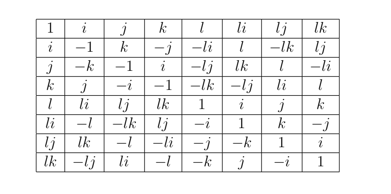
Figure 1: Multiplication table for the split octonions $\mathbb{O}^{\prime}$, from [4].

Using the decomposition $\mathbb{O}^{\prime}=\mathbb{H}\oplus l\mathbb{H}$, the signature (4,4) inner product $q$ is given by

$$q(a+lb,c+ld)\;=\;<a,c>_{\mathbb{H}}-<b,d>_{\mathbb{H}}$$

Write $q(u)=q(u,u)$ for the induced quadratic form. In the basis $\mathcal{M}$, set $u=\sum_{i=0}^{7}c_{i}m_{i}$, we have $q(u)=c_{0}^{2}+c_{1}^{2}+c_{2}^{2}+c_{3}^{2}-c_{4}^{2}-c_{5}^{2}-c_{6}^{2}-c_{7}^{2}$. In particular, the direct sum decomposition $\mathbb{O}^{\prime}=\mathbb{H}\oplus l\mathbb{H}$ is an orthogonal decomposition.

The split-octonions come with a special involution called a conjugation $*:\mathbb{O}^{\prime}\rightarrow\mathbb{O}^{\prime}$ which satisfies $x^{*}=x$ if and only if $x\in\mathbb{R}$. In particular, $\mathbb{O}^{\prime}$ splits orthogonally as $\mathbb{O}^{\prime}=\mathbb{R}\oplus\mathsf{Im}\,\mathbb{O}^{\prime}$, where $\mathsf{Im}\,\mathbb{O}^{\prime}$ is the imaginary split-octonions, the $(-1)$-eigenspace of $*$. The quadratic form $q$ is also given by

$$q(x)=xx^{*}.$$ (2.4)

Just as in the quaternions, $(xy)^{*}=y^{*}x^{*}$ for $x,y\in\mathbb{O}^{\prime}$. Now by definition, any $\varphi\in\mathsf{G}_{2}^{\mathbb{F}}$ satisfies $\varphi(1)=1$. Thus, it is standard to restrict the action of $\mathsf{G}_{2}^{\mathbb{F}}$ to $\mathsf{Im}\,\mathbb{O}^{\prime\mathbb{F}}$, where the representation is now irreducible. Moreover, $\mathfrak{g}_{2}$ admits no irreducible faithful representation on a vector space of dimension less than 7 [27].

The space $\mathsf{Im}\,\mathbb{O}^{\prime}$ is also endowed with a skew-symmetric map $\times:\mathsf{Im}\,\mathbb{O}^{\prime}\times\mathsf{Im}\,\mathbb{O}^{\prime}\rightarrow\mathsf{Im}\,\mathbb{O}^{\prime}$ defined by

$$x\times y:=x\odot y\;-\;q(x,y).$$ (2.5)

We call $\times$ a cross-product due to it satisfying the familar properties of $(\mathbb{R}^{3},\times_{\mathbb{R}^{3}})$. Namely, $\times$ is (i) bilinear, (ii) skew-symmetric, (iii) orthogonal (i.e. $x\times y\;\bot\;x,y$), and (iv) satisfies the normalization

$$q(x\times y)=q(x)q(y)-q(x,y)^{2}.$$ (2.6)

We will use often that (2.5) implies that $uv=u\times v$ when $u,v\in\mathsf{Im}\,\mathbb{O}^{\prime}$ are orthogonal.

Structures on $(\mathbb{O}^{\prime})^{\mathbb{C}}$.

We now define all the same structures on $(\mathbb{O}^{\prime})^{\mathbb{C}}$. The algebra $(\mathbb{O}^{\prime})^{\mathbb{C}}$ is equipped with the $\mathbb{C}$-bilinear extension $q_{\mathbb{C}}$ of the inner product $q$ on $\mathbb{O}^{\prime}$, the $\mathbb{C}$-linear extension of $*$, and the natural extension of $\odot$ to $(\mathbb{O}^{\prime})^{\mathbb{C}}=\mathbb{O}^{\prime}\otimes_{\mathbb{R}}\mathbb{C}$. The cross product on $\mathsf{Im}\,\mathbb{O}^{\prime\mathbb{C}}$ is then defined by the same equation (2.5) as in the real case, now using the multiplication and inner-product on $(\mathbb{O}^{\prime})^{\mathbb{C}}$. The cross-product on $(\mathbb{O}^{\prime})^{\mathbb{C}}$ also satisfies (i)-(iv). Finally, as a complexification of real vector space, $(\mathbb{O}^{\prime})^{\mathbb{C}}$ is equipped with a complex-conjugation $x\mapsto\overline{x}$ . For readability, we will fall back on the more standard notation of $\cdot$ to denote $q_{\mathsf{Im}\,\mathbb{O}^{\prime}}$ or $q_{\mathsf{Im}\,\mathbb{O}^{\prime}}^{\mathbb{C}}$ going forward.

There is one final crucial structure on $\mathbb{O}^{\prime}$: the scalar triple product $\Omega$ given by

$$\Omega(x,y,z)=(x\times y)\cdot z.$$ (2.7)

$\Omega$ is skew-symmetric due to the skew-symmetry of $\times$ and the symmetry of $q$. More surprisingly, $\Omega$ provides a calibration in the sense of Harvey & Lawson [34] and is intimately related to $\mathsf{G}_{2}^{\mathbb{F}}$ geometry. In fact, $\mathsf{G}_{2}^{\prime}$ can be defined in terms of $\Omega$, as we note below.

We will use the following non-trivially equivalent characterizations of $\mathsf{G}_{2}^{\prime}$ as groups of linear transformations [27]:

1. Split-octonion algebra product automorphisms: $\{\psi\in\mathsf{GL}(\mathbb{O}^{\prime})\;|\;\psi(x\odot y)=\psi(x)\odot\psi(y)\}$, transformations which turn out to automatically also preserve $\times,q,*$.

2. Cross-product preserving transformations: $\{\psi\in\mathsf{GL}(\mathsf{Im}\,\mathbb{O}^{\prime})\;|\;\psi(x\times y)=\psi(x)\times\psi(y)\}$.

3. Stabilizing transformations of $\Omega:\{\psi\in\mathsf{GL}(\mathsf{Im}\,\mathbb{O}^{\prime})\;|\;\psi^{*}\Omega=\Omega\}$.

2.2 Some $\mathbb{O}^{\prime}$ Identities

We record the following identities, which we learned the excellent text [27], for future use.

The double cross-product identity holds for any $x,y\in\mathsf{Im}\,\mathbb{O}^{\prime}$.

$$x\times(x\times y)=(x\cdot y)\,x-q(x)\,y.$$ (2.8)

When applied thrice to $x=z+w$, the previous identity gives us the generalized double cross-product identity.

$$z\times(w\times y)+w\times(z\times y)=(z\cdot y)w+(w\cdot y)z-2(z\cdot w)\,y.$$ (2.9)

A very useful corollary to (2.9) occurs in the case that $x,y,z$ are pairwise orthogonal. Indeed, in this case,

$$x\times(y\times z)=-y\times(x\times z).$$ (2.10)

Finally, we note a very useful orthogonality property of the cross product.

Lemma 2.1 (Orthogonality of Cross-Product).

Let $u,v,w\in\mathsf{Im}\,\mathbb{O}^{\prime}$ be pairwise orthogonal. Then $(w\times u)\;\bot(w\times v)$.

2.3 $\hat{\mathbb{S}}^{2,4}$ and its Almost-Complex Structure.

We now define $\hat{\mathbb{S}}^{2,4}:=\{\,x\in\mathsf{Im}\,\mathbb{O}^{\prime}\;|\,q(x)=+1\}$ as the unit sphere in the imaginary split-octonions. The space $\hat{\mathbb{S}}^{2,4}$ is a 2-1 cover of $\mathbb{S}^{2,4}:=\{[x]\in\mathbb{P}\mathsf{Im}\,\mathbb{O}^{\prime}\;|\;q(x)>0\}$ of the space of positive-definite lines. We may use the projective model $\mathbb{S}^{2,4}$ later.

We begin by identifying $T_{x}\hat{\mathbb{S}}^{2,4}\cong[x^{\bot}\subset\mathsf{Im}\,\mathbb{O}^{\prime}]$. Then $q_{\mathbb{O}^{\prime}}$ defines a $\mathsf{G}_{2}^{\prime}$-invariant signature (2,4) pseudo-Riemannian metric on $\hat{\mathbb{S}}^{2,4}$. The natural almost-complex structure $J$ on $\mathsf{Im}\,\mathbb{O}^{\prime}$ comes from the cross-product $\times$. Recall here that an almost-complex structure on a manifold $M$ is a bundle endomorphism $J:TM\lcirclearrowleft$ satisfying $J^{2}=-\text{id}$. Moreover, an almost-complex curve is a map $\phi:(M,J_{M})\rightarrow(X,J_{X})$ satisfying $d\phi\circ J_{M}=J_{X}\circ d\phi$.

We now define $J$. First, take a position vector $w\in\hat{\mathbb{S}}^{2,4}$ and denote $C_{w}:=(v\mapsto w\times v)$ as the cross-product map associated to $w\in\mathsf{Im}\,\mathbb{O}^{\prime}$. The double cross-product identity (2.8) implies $(C_{w}\circ C_{w})|_{w^{\bot}}=-\mathsf{id}_{w^{\bot}}$. Hence, $J$ is given pointwise by $J_{w}:T_{w}\mathbb{S}^{2,4}\rightarrow T_{w}\mathbb{S}^{2,4}$ via $J_{w}:=C_{w}$, or

$$J_{w}(u)=w\times u.$$ (2.11)

The paper [56] asserts that $J_{\hat{\mathbb{S}}^{2,4}}$ is non-integrable and moreover admits no 4-dimensional almost-complex submanifolds, as was the case for the canonical almost-complex structure $J_{\mathbb{S}^{6}}$.

A First Stiefel Model for $\mathsf{G}_{2}^{\prime}$.

We now finish the preliminaries by providing a Stiefel-manifold description of $\mathsf{G}_{2}^{\prime}$, which will be useful in the construction of the almost-complex curve in Section 3. The following idea of finding bases of $\mathsf{Im}\,\mathbb{O}^{\prime}$ from special triplets is not new, but is a particularly convenient way to think about $\mathsf{G}_{2}$ [3, 27, 34, 52]. The following proposition tells us we can think of $\mathsf{G}_{2}^{\prime}$ as the collection of all algebra bases of $\mathbb{O}^{\prime}$ satisfying the same relations as $i,j,l$. To this end, we define:

Definition 2.2.

We call a basis $\mathcal{F}=(f_{i})_{i=1}^{7}$ for $\mathsf{Im}\,\mathbb{O}^{\prime}$ a multiplication basis when $\mathcal{F}=\varphi(\mathcal{M})$ for $\varphi\in\mathsf{G}_{2}$, where $\mathcal{M}$ is the standard multiplication basis (2.3). That is, $\mathcal{F}$ is a multiplication basis when the linear map $\varphi:=(m_{i}\mapsto f_{i})$ preserves the cross-product.

We provide the following proof to provide some feeling for $\mathsf{G}_{2}^{\prime}$. Note that the signs in the subscript refer to the $q_{\mathbb{O}}$-norm of the triplets. Indeed, $q_{\mathsf{Im}\,\mathbb{O}^{\prime}}(x)=-x^{2}$, so for $x\in\mathsf{Im}\,\mathbb{O}^{\prime}$, $x^{2}=\pm 1$ if and only if $q(x)=\mp 1$.

Proposition 2.3 ( $(+,+,-)$ Stiefel Description of $\mathsf{G}_{2}^{\prime}$).

Consider the set

$$V_{(+,+,-)}(\mathsf{Im}\,\mathbb{O}^{\prime}):=\,\{\,(x,y,z)\;|\;\;x,y,z\in\mathsf{Im}\,\mathbb{O}^{\prime},\;x^{2}=y^{2}=-1,\;z^{2}=1,\;\,x\cdot y\,=\,x\cdot z=\,y\cdot z=0,\;z\,\cdot\,(x\times y)=0\;\}$$

of (ordered) orthonormal triplets. Then $\mathsf{G}_{2}^{\prime}$ acts transitively, without fixed points on $V_{(+,+,-)}(\mathsf{Im}\,\mathbb{O}^{\prime})$.

Proof.

Given any triplet $p=(x,y,z)\in V_{(+,+,-)}(\mathsf{Im}\,\mathbb{O}^{\prime})$, one naturally creates an orthonormal (ordered) vector space basis $\mathcal{B}=(b_{i})_{i=1}^{7}$ for $\mathsf{Im}\,\mathbb{O}^{\prime}$ in the same way we get $\mathcal{M}$, (2.3), from $i,j,l$. Namely,

$$\mathcal{B}=(x,y,xy,z,zx,zy,z(xy)).$$ (2.12)

We consider the linear map $\varphi:=m_{i}\mapsto b_{i}$. In particular, $\varphi(i)=x,\varphi(j)=y,\varphi(l)=z$. If we can show $\varphi\in\mathsf{G}_{2}^{\prime}$, then $\mathsf{G}_{2}^{\prime}$ acts transitively on $V_{(+,+,-)}$.

To prove $\varphi\in\mathsf{G}_{2}^{\prime}$, one can use some general identities of $\mathbb{O}^{\prime}$, adapting the argument of Lemma A.8 of [34]. By the orthogonality property $(x\times y)\cdot z=0$, if we define the copy of the quaternions $H:=\mathsf{span}_{\mathbb{R}-\mathsf{alg}}<x,y>$, then $z\in H^{\bot}$. Then the Lemma A.8 of [34] tells us that for $a,b,c,d\in H$,

$$(a+zb)(c+zd)=ac+db^{*}+z(a^{*}d+cb).$$ (2.13)

We will see that this identity implies $\varphi\in\mathsf{G}_{2}^{\prime}$. Now, the fact that $\mathcal{B}$ is a basis implies we have a direct sum decomposition $\mathbb{O}^{\prime}=H\oplus zH$. Then equation (2.13) says that if we take $(a,b)\in H\oplus H$ corresponding to $a+zb$, then the multiplication of $\mathbb{O}^{\prime}$ in this model is given by exactly the formula (2.1). In particular, the map $\varphi$ preserves $\odot$. We conclude that $\mathsf{G}_{2}^{\prime}$ acts transitively on $V_{(+,+,-)}(\mathsf{Im}\,\mathbb{O}^{\prime})$. On the other hand, suppose $\varphi,\psi\in\mathsf{G}_{2}^{\prime}$ act with $\varphi\cdot p=q,\;\psi\cdot p=q$ for $p,q\in V_{(+,+,-)}(\mathsf{Im}\,\mathbb{O}^{\prime})$, then one finds $\psi(\mathcal{B}_{p})=\varphi(\mathcal{B}_{p})=\mathcal{B}_{q}$ for the basis creation process (2.12) since $\varphi$ preserves multiplication. But then $\varphi=\psi$ by linearity. Hence, the action of $\mathsf{G}_{2}^{\prime}$ on $V_{(+,+,-)}$ has no fixed points. ∎

As a corollary to the proof, we learn the following:

Corollary 2.4 ($\mathsf{G}_{2}^{\prime}$ and Multiplication Frames).

The group $\mathsf{G}_{2}^{\prime}$ acts transitively, without fixed points on the space of multiplication frames for $\mathsf{Im}\,\mathbb{O}^{\prime}$.

Corollary 2.5 ($\mathsf{G}_{2}^{\prime}$ and $\hat{\mathbb{S}}^{2,4}$).

$\mathsf{G}_{2}^{\prime}$ acts transitively (and isometrically) on $\hat{\mathbb{S}}^{2,4}$.

2.4 A Complex Cross-Product Basis for $(\mathsf{Im}\,\mathbb{O}^{\prime})^{\mathbb{C}}$

Following Baraglia [4], we will use the following carefully selected basis
$\mathcal{B}=(u_{3},u_{2},u_{1},u_{0},u_{-1},u_{-2},u_{-3})$ for $\mathsf{Im}\,\mathbb{O}^{\prime\mathbb{C}}$. The basis $(u_{i})_{i=3}^{-3}$ will be extremely useful for understanding almost-complex curves in $\mathbb{S}^{2,4}$ in Section 3. The name ‘complex cross-product basis’ is motivated by property (3) of Proposition 2.6.

$$\begin{cases}u_{3}&=\frac{1}{\sqrt{2}}(\,jl+\sqrt{-1}kl).\\ u_{2}&=\frac{1}{\sqrt{2}}(\,j+\sqrt{-1}k).\\ u_{1}&=\frac{1}{\sqrt{2}}(\,l+\sqrt{-1}il).\\ u_{0}&=i.\\ u_{-1}&=\frac{1}{\sqrt{2}}(\,l-\sqrt{-1}il).\\ u_{-2}&=\frac{1}{\sqrt{2}}(\,j-\sqrt{-1}k).\\ u_{-3}&=\frac{1}{\sqrt{2}}(\,jl-\sqrt{-1}kl).\end{cases}$$ (2.14)

Observe that $u_{-i}=\overline{u_{i}}$, where $x\mapsto\overline{x}$ denotes complex conjugation with respect to the standard complex structure on $(\mathbb{O}^{\prime})^{\mathbb{C}}$. We state all of the useful properties of $\mathcal{B}$ we know, of which only (1) is given in [4].

Proposition 2.6 (Properties of Complex Cross-Product Basis).

The basis $\mathcal{B}$ satisfies:

1. The inner-product with respect to $\mathcal{B}$ is given by

   $$q_{\mathbb{C}}(\mathbf{x},\mathbf{y})=\mathbf{x}^{T}\;\begin{pmatrix}&&&&&&-1\\ &&&&&1&\\ &&&&-1&&\\ &&&1&&&\\ &&-1&&&&\\ &1&&&&&\\ -1&&&&&&\end{pmatrix}\;\mathbf{y},$$ (2.15)

2. Define the operator $C_{u_{0}}:\mathsf{Im}\,\mathbb{O}^{\prime\mathbb{C}}\rightarrow\mathsf{Im}\,\mathbb{O}^{\prime\mathbb{C}}$ by $C_{u_{0}}:=(u_{0}\times\,\cdot)$. Then the $\pm\sqrt{-1}$ eigenspaces are given by

   $$\mathbb{E}_{\sqrt{-1}}(C_{u_{0}})=\mathsf{span}_{\mathbb{C}}<u_{3},u_{-2},u_{-1}>\;\;\text{and}\;\;\mathbb{E}_{-\sqrt{-1}}(C_{u_{0}})=\mathsf{span}_{\mathbb{C}}<u_{-3},u_{2},u_{1}>.$$

3. More generally, we have $u_{i}\times u_{j}=C_{ij}u_{i+j}$ for constants $C_{ij}\in\mathbb{C}$, possibly 0, where we set $u_{i}=0$ for $|i|>3$.

4. For constants $C_{ijk}\in\mathbb{C}$, the 3-form $\Omega$ in the basis $\mathcal{B}$ has the form

   $$\Omega=\sum_{i+j+k=0}C_{ijk}\,u_{i}^{*}\wedge u_{j}^{*}\wedge u_{k}^{*}.$$ (2.16)

5. A transformation $D\in\mathsf{GL}(\mathsf{Im}\,\mathbb{O}^{\prime\mathbb{C}})$ of the form $D=\mathsf{diag}(d_{i})_{i=3}^{-3}$ in the basis $\mathcal{B}$ satisfies $D\in\mathsf{G}_{2}^{\mathbb{C}}$ if and only if $d_{i}d_{j}d_{k}=1$ for all pairwise distinct triplets $(i,j,k)$ such that $i+j+k=0$.

Proof.

We sketch the proof. First, using that $q_{\mathsf{Im}\,\mathbb{O}^{\prime}}=\mathsf{diag}(+1,+1,+1,-1,-1,-1,-1)$ in the basis $\mathcal{M}=(m_{i})_{i=1}^{7}$, one can directly compute that (1) is the correct expression for $q_{\mathsf{Im}\,\mathbb{O}^{\prime}}^{\mathbb{C}}$ with respect to $\mathcal{B}$. For example, it is immediately evident that $u_{i}\cdot u_{j}=0$ for $j\notin\{-i,+i\}$.

We can see (2) by direct calculation, using that $C_{u_{0}}$ acts as the standard complex structure $\begin{pmatrix}0&-1\\ 1&0\end{pmatrix}$ on the 2-planes $\mathsf{span}_{\mathbb{R}}<m_{2},m_{3}>,\mathsf{span}_{\mathbb{R}}<m_{4},m_{5}>,\mathsf{span}_{\mathbb{R}}<m_{6},m_{7}>$ in the ordered bases $(m_{2},m_{3}),\,(m_{5},m_{4}),\,(m_{7},m_{6})$, respectively.

(3) is a tedious and direct calculation. In Appendix B we give all the multiplicative relations amongst the basis elements. We remark that since $u_{-i}=\overline{u}_{i}$ and $\overline{xy}=\overline{x}\;\overline{y}$ for $x,y\in(\mathbb{O}^{\prime})^{\mathbb{C}}$, the relation relation $u_{i}\times u_{j}=C_{ijk}u_{k}$ for $C_{ijk}\in\mathbb{C}$ is equivalent to the relation $u_{-i}\times u_{-j}=\overline{C_{ijk}}u_{-k}$.

(5) is an immediate consequence of (4). If $D$ is diagonal, then $D$ preserves $\Omega$ iff it preserves each decomposable tensor $u^{i,j,k}$ and the claim follows. ∎

Remark 2.7.

Later, we use an analogous basis called a ‘real cross-product basis’ in Section 8.3, adapted to the real vector space $\mathsf{Im}\,\mathbb{O}^{\prime}$.

2.5 A Model for $\mathfrak{g}_{2}$.

Recall that $\mathsf{G}_{2}^{\mathbb{F}}=\{\psi\in\mathsf{GL}(\mathsf{Im}\,\mathbb{O}^{\prime\mathbb{F}})\;|\;\psi(u\times v)=u\times v\}$. Consequently, the Lie algebra $\mathfrak{g}_{2}^{\mathbb{F}}$ is the set of transformations infinitesimally preserving the cross-product, i.e., derivations of the cross product:

$$\mathfrak{g}_{2}^{\mathbb{F}}=\{\,A\in\mathsf{End}(\mathsf{Im}\,\mathbb{O}^{\prime\mathbb{C}})\;|\;A(x\times y)=(A\,x)\times y+x\times(Ay)\;\}$$

For symmetry of notation, we later write $\mathfrak{g}_{2}^{\prime}:=\mathfrak{g}_{2}^{\mathbb{R}}$. Fixing the (ordered) basis $\mathcal{B}:=(u_{i})_{i=3}^{-3}$ for $\mathsf{Im}\,\mathbb{O}^{\prime\mathbb{C}}$, we obtain a matrix representation $\Psi$ of $\mathfrak{g}_{2}$ by writing these endomorphisms with respect to $\mathcal{B}$. In short, $\Psi:\mathfrak{g}_{2}\rightarrow\mathfrak{gl}_{7}\mathbb{C}$ by $A\;\stackrel{{\scriptstyle\Psi}}{{\longmapsto}}\;[A]_{\mathcal{B}}$. Going forward, we will conflate $\mathfrak{g}_{2}$ with its image under this representation $\Psi$. When we use a different basis for $\mathsf{Im}\,\mathbb{O}^{\prime\mathbb{C}}$, we will make this clear.

For completeness, we include the full details of $\mathfrak{g}_{2}$ Lie theory in the basis $\mathcal{B}$ in the Appendix. Specifically, Section A.1 contains the root space decomposition, Section A.3 contains our choice of model principal 3-dimensional subalgebra $\mathfrak{s}$ of Kostant [43], and Section A.4 contains the Cartan involution $\sigma$ from [36].

2.6 Cyclic $\mathsf{G}_{2}$ Higgs Bundles

We now form the Higgs bundle $\mathcal{E}$ in which we work for most of the paper. Denote $\mathcal{K}$ as the holomorphic cotangent bundle of $\mathbb{C}$ and we fix the holomorphic vector bundle

$$\mathcal{E}=\mathcal{K}^{3}\oplus\mathcal{K}^{2}\oplus\mathcal{K}\oplus\mathcal{O}\oplus\mathcal{K}^{-1}\oplus\mathcal{K}^{-2}\oplus\mathcal{K}^{-3}.$$ (2.17)

We place an orthogonal structure $E$ on the bundle by taking a coordinate vector $\mathbf{x}=(x_{i})_{i=3}^{-3}$ in the basis $(dz^{i})_{i=3}^{-3}$ and forming the metric

$$E(\mathbf{x},\mathbf{y})=\mathbf{x}^{T}R\,\mathbf{y},$$

where

$$R=\begin{pmatrix}&&&&&&-1\\ &&&&&1&\\ &&&&-1&&\\ &&&1&&&\\ &&-1&&&&\\ &1&&&&&&\\ -1&&&&&&\end{pmatrix}.$$

Then $E$ reduces the structure group of $\mathcal{E}$ to $\mathsf{SO}_{7}\mathbb{C}$. We then further reduce the structure group by identifying our $\mathbb{C}^{7}$ fibers with $\mathsf{Im}\,\mathbb{O}^{\prime\mathbb{C}}$ as follows. Let $(\mathbf{e}_{3},\mathbf{e}_{2},\mathbf{e}_{1},\mathbf{e}_{0},\mathbf{e}_{-1},\mathbf{e}_{-2},\mathbf{e}_{-3})$ be the standard basis of $\mathbb{C}^{7}$, indexed to match the powers of $\mathcal{K}$. We fix once-and-for-all the identification of the fibers of $\mathcal{E}$ with complex split-octonions by identifying $\mathbf{e}_{i}$ with $u_{i}\in\mathcal{B}$ from our complex cross-product basis from Proposition 2.14. By equation (2.15), this identification respects our initial choice of orthogonal structure. That is to say, the $\mathsf{Im}\,\mathbb{O}^{\prime}$ dot-product $q$ in the basis $(u_{i})_{i=3}^{-3}$ is the same as is the dot-product $E$ in the basis $(\mathbf{e}_{i})_{i=3}^{-3}$. This identification $\mathbf{e}_{i}\leftrightarrow u_{i}$ defines a reduction of structure to $\mathsf{G}_{2}$ by considering only frames that preserve the $(\mathsf{Im}\,\mathbb{O}^{\prime})^{\mathbb{C}}$ cross-product.

Remark 2.8.

We emphasize that the identification of fibers of $\mathcal{E}_{\Sigma}:=\bigoplus_{i=3}^{-3}\mathcal{K}_{\Sigma}^{i}$ with $(\mathsf{Im}\,\mathbb{O}^{\prime})^{\mathbb{C}}$ extends to any Riemann surface to give a reduction of structure to $\mathsf{G}_{2}$. Let $(z_{\alpha},U_{\alpha})$ be an atlas for $\Sigma$. Then applying the aforementioned identification $dz_{\alpha}^{i}\leftrightarrow u_{i}$ in the local holomorphic frames $\mathcal{B}_{\alpha}=(dz_{\alpha}^{i})_{i=3}^{-3}$, one finds that the local transitions are in $\mathsf{G}_{2}$, i.e., they respect the cross-product $\times$ on $(\mathsf{Im}\,\mathbb{O}^{\prime})^{\mathbb{C}}$. Indeed, if $z_{\beta}=g_{\alpha\beta}z_{\alpha}$, then set $\zeta:=\frac{\partial g_{\alpha\beta}}{\partial z_{\alpha}}$ and we have $\mathcal{B}_{\beta}=\psi\,\mathcal{B}_{\alpha}$, where

$$\psi=\mathsf{diag}(\zeta^{3},\zeta^{2},\zeta^{1},1,\zeta^{-1},\zeta^{-2},\zeta^{-3}).$$

By Proposition 2.6 part (5), $\psi\in\mathsf{G}_{2}$. Thus, these local identifications yield a globally well-defined bundle map $\times_{\mathcal{E}}:\mathcal{E}\times\mathcal{E}\rightarrow\mathcal{E}$ defined by using any of the local cross products.

The (Kostant) invariants of $\mathfrak{g}_{2}$ are 1 and 5. Thus, the $\mathsf{G}_{2}$ Hitchin component is parametrized by pairs of holomorphic quadratic and sextic differentials $q_{2},q_{6}$. Since we are interested in only cyclic Higgs bundles, we set $q_{2}=0$ and denote $q:=q_{6}$. Following Hitchin [36], our Higgs field is of the form $\varphi=\tilde{e}+qe_{\gamma}$, where $\tilde{e}$ comes from our distinguished principal Kostant 3DS $\mathfrak{s}=\mathsf{span}_{\mathbb{C}}<x,e,\tilde{e}>$ and $e_{\gamma}$ is the (normalized) highest weight vector given by

$$e_{\gamma}=\begin{pmatrix}0&&&&&1&\\ &0&&&&&1\\ &&0&&&&\\ &&&0&&&\\ &&&&0&&\\ &&&&&0&\\ &&&&&&0\\ \end{pmatrix}.$$

Thus, the Higgs field in these coordinates is

$$\varphi =\begin{pmatrix}0&&&&&q&\\ \sqrt{3}&0&&&&&q\\ &\sqrt{5}&0&&&&\\ &&-\sqrt{-6}&0&&&\\ &&&-\sqrt{-6}&0&&\\ &&&&\sqrt{5}&0&\\ &&&&&\sqrt{3}&0\\ \end{pmatrix}.$$ (2.18)

2.6.1 Harmonic Metric & Hitchin’s Equation

We now search for a Hermitian metric $h$ on $\mathcal{E}$ such that the connection $\nabla=\nabla_{\overline{\partial},h}+\varphi+\varphi^{*h}$ flat. The flatness of $\nabla$ is equivalent to the metric $h$ satisfying Hitchin’s equations [36].

$$F_{h}+[\varphi,\varphi^{*h}] =0.$$ (2.19)

$$\nabla_{h,\overline{\partial}}^{0,1}\,\varphi =0.$$ (2.20)

Here, $F_{h}$ is the curvature of the Chern connection $\nabla_{\overline{\partial},h}$. By our construction of the Higgs field, equation (2.20) is equivalent to the holomorphicity of $q$. Due to our interest in cyclic Higgs bundles, we look for a metric $h$ that is diagonal in the standard holomorphic coordinates [4]. Let $r,s>0$ be positive functions. Then in the standard coordinates $(dz^{i})_{i=3}^{-3}$, we search for $h$ of the form

$$h(\mathbf{x},\mathbf{y})=\mathbf{\overline{x}}^{T}\,\mathsf{diag}(r^{-1}s^{-1},r^{-1},s^{-1},1,s,r,rs)\,\mathbf{y}=\mathbf{\overline{x}}^{T}\,H\,\mathbf{y}.$$ (2.21)

Now, the $h$-adjoint of $\varphi$ is given by $\varphi^{*h}=H^{-1}\overline{\varphi}^{T}H$. Thus,

$$\varphi^{*h} =\begin{pmatrix}0&\sqrt{3}\,s&&&&&\\ &0&\sqrt{5}\frac{r}{s}&&&&\\ &&0&\sqrt{-6}s&&&\\ &&&0&\sqrt{-6}s&&\\ &&&&0&\sqrt{5}\frac{r}{s}&\\ \frac{\overline{q}}{r^{2}s}&&&&&0&\sqrt{3}\,s\\ &\frac{\overline{q}}{r^{2}s}&&&&&0\\ \end{pmatrix}.$$ (2.22)

The curvature of the Chern connection is $F_{h}=\overline{\partial}(H^{-1}\partial H)=(\log H)_{z\bar{z}}\;d\bar{z}\wedge dz.$ Writing $\varphi=\widehat{\varphi}\,dz,\varphi^{*h}=\widehat{\varphi^{*h}}d\bar{z}$, Hitchin’s equation (2.19) becomes a pointwise equation

$$(\log H)_{z\bar{z}}d\bar{z}\wedge dz=[\widehat{\varphi},\widehat{\varphi^{*h}}]d\bar{z}\wedge dz.$$ (2.23)

Taking the second and third components along the diagonal, equation (2.19) is equivalent to the following $2\times 2$ coupled system of PDE for $r,s$. We use $\Delta:=\partial_{\bar{z}}\circ\partial_{z}$ going forward.

$$\begin{cases}\Delta\log r&=5\frac{r}{s}-3s-\,\frac{|q|^{2}}{r^{2}s}\\ \Delta\log s&=6s-5\frac{r}{s}.\end{cases}$$ (2.24)

Substituting $u_{1}=\log r+\frac{1}{2}\log s$, $v_{1}=\frac{1}{2}\log s$, the system (2.24) becomes

$$\begin{cases}2\Delta u_{1}&=5e^{(u_{1}-3u_{2})}-2e^{-2u_{1}}\,|q|^{2}.\\ 2\Delta u_{2}&=6e^{2u_{2}}-5e^{(u_{1}-3u_{2})}.\end{cases}$$ (2.25)

Later, it will be useful to have a form of these equations with the constants all equal. Hence, define $c,d>0\in\mathbb{R}$ which uniquely solve the system

$$\begin{cases}5c^{5/6}d^{-1/2}-2c^{-5/3}&=0\\ -5c^{5/6}d^{-1/2}+6d^{1/3}&=0.\end{cases}$$ (2.26)

The exact solution to (2.26) is $d=\frac{5}{6\sqrt{3}},c=(\frac{2}{5})^{2/5}d^{1/5}.$

Define $b=\frac{6d^{1/3}}{2}$. Then $\boldsymbol{w}$ solves (2.27) if and only if $\boldsymbol{u}$ solves (2.25), where $u_{1}=w_{1}+\log(c^{5/6})$ and $u_{2}=w_{2}+\log(d^{1/6})$.

$$\begin{cases}\Delta w_{1}&=b\left(e^{(w_{1}-3w_{2})}-e^{-2w_{1}}\,|q|^{2}\right)\\ \Delta w_{2}&=b\left(e^{2w_{2}}-e^{(w_{1}-3w_{2})}\right).\end{cases}$$ (2.27)

For later purposes, we also re-write the system (2.25) with respect to a different metric $\sigma=\sigma(z)|dz|^{2}$. Given a solution $\boldsymbol{u}$ of (2.25), we define $\boldsymbol{\psi}=(\psi_{1},\psi_{2})$ by

$$\begin{cases}e^{\psi_{1}}\sigma^{5/2}&=e^{u_{1}}\\ e^{\psi_{2}}\sigma^{1/2}&=e^{u_{2}}.\end{cases}$$

A calculation shows that $\boldsymbol{\psi}$ solves the system (2.28):

$$\begin{cases}2\Delta_{\sigma}\psi_{1}&=5e^{\psi_{1}-3\psi_{2}}-2|q|^{2}_{\sigma}\,e^{-2\psi_{1}}+\frac{5}{2}\kappa_{\sigma}\\ 2\Delta_{\sigma}\psi_{2}&=-5e^{\psi_{1}-3\psi_{2}}+6e^{2\psi_{2}}+\frac{1}{2}\kappa_{\sigma}\end{cases},$$ (2.28)

where $|q|^{2}_{\sigma}:=\frac{q\bar{q}}{\sigma^{6}}$ and $\kappa_{\sigma}=\frac{2}{\sigma}\Delta\log\sigma$.

Relation to $\mathfrak{sl}_{6}\mathbb{C}$ affine Toda Equations. We now explain why there is no naive linear equivalence between the $\mathfrak{g}_{2}$ affine Toda equations and the $\mathfrak{sl}_{n}\mathbb{C}$ affine Toda equations. The affine Toda equations for $\mathfrak{sl}_{n}\mathbb{C}$ depend on a holomorphic differential $q\in H^{0}(\mathcal{K}^{n}_{\mathbb{C}})$. While one might expect the $\mathfrak{sl}_{7}\mathbb{C}$ Toda equations to coincide with the $\mathfrak{g}_{2}$ Toda equations, the orders of the differentials do not match. The only natural candidate to compare the $\mathfrak{g}_{2}$ affine Toda equations to is the $\mathfrak{sl}_{6}\mathbb{C}$ affine Toda equations. Now, take $q\in H^{0}(\mathcal{K}^{6}_{\mathbb{C}})$ polynomial. By [48], any complete solution to the $\mathfrak{sl}_{6}\mathbb{C}$ equations is real. It now suffices for us to see the $\mathfrak{sl}_{6}\mathbb{C}$ and $\mathfrak{g}_{2}$ equations are not equivalent away from the zeros of $q$. We therefore discuss the equations in a natural coordinate $w$ for $q$ where $q=dw^{6}$. A real $\mathfrak{sl}_{6}\mathbb{C}$ solution $\boldsymbol{u}=(u_{1},u_{2},u_{3})$ is a solution to (c.f. equation (10) [48])

$$\begin{cases}\Delta u_{1}&=e^{u_{1}-u_{2}}-e^{-2u_{1}}\\ \Delta u_{2}&=e^{u_{2}-u_{3}}-e^{u_{1}-u_{2}}\\ \Delta u_{3}&=e^{2u_{2}}-e^{u_{2}-u_{3}}.\end{cases}$$ (2.29)

On the other hand, for $\mathfrak{g}_{2}$, a real solution is a solution to the system

$$\begin{cases}2\Delta w_{1}&=5e^{w_{1}-3w_{2}}-2e^{-2w_{1}}\\ 2\Delta w_{2}&=6e^{2w_{2}}-5e^{w_{1}-3w_{2}}.\\ \end{cases}$$ (2.30)

We explain now why these equations should not be (naively) linearly equivalent. That is, there do not exist constants $a_{i},b_{i},c_{i}\in\mathbb{R}$ such that for any solution $\boldsymbol{w}=(w_{1},w_{2})$ of (2.30), then $\boldsymbol{u}=(u_{1},u_{2},u_{3})$ solves to (2.29), where $u_{i}=a_{i}w_{1}+b_{i}w_{2}+c_{i}\;(*)$. Suppose, for contradiction, such constants exist. Take $\boldsymbol{w}$ a solution (2.30), and define $\boldsymbol{u}$ as in $(*)$. Then the following system of equations holds:

$$\begin{cases}e^{u_{1}-u_{2}}-e^{-2u_{1}}&=\Delta u_{1}=\frac{5}{2}(a_{1}-b_{1})e^{w_{1}-3w_{2}}-a_{1}\,e^{-2w_{1}}+3b_{1}\,e^{2w_{2}}\\ e^{u_{2}-u_{3}}-e^{u_{1}-u_{2}}&=\Delta u_{2}=\frac{5}{2}(a_{2}-b_{2})e^{w_{1}-3w_{2}}-a_{2}\,e^{-2w_{1}}+3b_{2}\,e^{2w_{2}}\\ e^{2u_{3}}-e^{u_{2}-u_{3}}&=\Delta u_{3}=\frac{5}{2}(a_{3}-b_{3})e^{w_{1}-3w_{2}}-a_{3}\,e^{-2w_{1}}+3b_{3}\,e^{2w_{2}}.\end{cases}$$ (2.31)

We show that there is no way for term-by-term matching to occur on both sides of (2.31). Indeed, if term-by-term matching were to occur, then for $i\in\{1,2,3\}$, we have exactly one of the following: $a_{i}=b_{i},a_{i}=0,$ or $b_{i}=0$. We handle these 3 cases now. The choices for $a_{1},b_{1},c_{1}$ in each case cascade to force choices for $a_{i},b_{i},c_{i}$ for $i>1$ and such choices fail to make $\boldsymbol{u}$ solve (2.29).

Case 1: $a_{1}-b_{1}=0$. Set $a:=a_{1}=b_{1}$ by hypothesis. Then $e^{-2u_{1}}=Ce^{-aw_{1}-aw_{2}}$. But for no choice of $a\in\mathbb{R}$ is $\{-aw_{1}-aw_{2}\}\in\{w_{1}-3w_{2},\,-2w_{1},\,2w_{2}\}$. Hence, the terms cannot match.

Case 2: $a_{1}=0$. Examining the exponents similarly, $u_{1}=-w_{2}+c_{1}$ is forced. To match the term $e^{u_{1}-u_{2}}$ to a term on the right-hand side, one finds $u_{2}=2w_{2}-w_{1}+c_{2}$. But then all 3 terms on the right-hand side of (2.31) for $\Delta u_{2}$ are nonzero, a contradiction to term matching.

Case 3: $b_{1}=0$. Then $u_{1}=a_{1}w_{1}+c_{1}$. To match terms, we must have $-e^{-2u_{1}}=-e^{-2w_{1}}$, so that $a_{1}=1$. But then $e^{u_{1}-u_{2}}=C\,e^{w_{1}-3w_{2}}$, so that $u_{2}=3w_{2}+c_{2}$ is forced. Hence, $a_{2}=0$. This means $e^{u_{2}-u_{3}}=C^{\prime}\,e^{2w_{2}}$, so $u_{3}=w_{3}+c_{3}$ and $a_{3}=0$. We examine the final equation. By the exponents, we must have $e^{2u_{3}}=3b_{3}e^{w_{2}}$ and hence

$$-e^{w_{2}+(c_{2}-c_{3})}=-e^{u_{2}-u_{3}}=-\frac{5}{2}\,e^{w_{1}-3w_{2}},$$

so that the exponents are wrong in the final term. We conclude that there is no obvious linear substitution for which real solutions to (2.30) are also real solutions to (2.29).

2.6.2 Parabolic Structure

We now define a parabolic structure on $\mathcal{E}$. Take a section $s=s_{i}dz^{i}\in\Gamma(\mathbb{C},\mathcal{E})$ that is meromorphic in the usual sense, i.e., each $s_{i}$ is meromorphic. Define $(s_{i})_{\infty}\in\mathbb{Z}$ as the order of $s_{i}$ at $\infty$. We then define a parabolic structure on $\mathcal{E}$ as follows. We define weights $(\alpha_{i})_{i=3}^{-3}:=(-\frac{n}{2},-\frac{n}{3},-\frac{n}{6},0,\frac{n}{6},\frac{n}{3},\frac{n}{2})$. For each meromorphic section $s\in\Gamma(\mathbb{C},\mathcal{E})$, we define the order at infinity by

$$v_{\infty}(s):=\max_{-3\leq i\leq 3}\{(s_{i})_{\infty}+\alpha_{i}\}.$$

We can explain where this definition comes from by noting the asymptotics proven later for the metric $h=\mathsf{diag}(\frac{1}{rs},\frac{1}{r},\frac{1}{s},1,s,r,rs)$ on $\mathcal{E}$ in the standard frame $(dz_{i})_{i=3}^{-3}$. We prove that $r\asymp|q|^{2/3}\asymp|z|^{\frac{2n}{3}}$ and $s\asymp|q|^{\frac{1}{3}}\asymp|z|^{\frac{n}{3}}$, where $q$ is a monic polynomial of degree $n$, by Theorem 5.5, using our sub and super-solutions from Lemmas 5.3, 5.2. We write $f(z)\asymp g(z)$ here to denote asymptotically comparable in the sense that $f(z)\in O(g(z))$ and $g(z)\in O(f(z))$.

In particular, the asymptotics for $r,s$ imply that the canonical section $\sigma_{i}:=dz^{i}\in\Gamma(\mathbb{C},\mathcal{K}_{\mathbb{C}}^{i})$ satisfies that $h(\sigma_{i},\sigma_{i})\asymp|z|^{2\alpha_{i}}$ for the aforementioned constants $\alpha_{i}$. Thus, the metric $h$ respects the parabolic structure in the sense that for any meromorphic section $s\in\Gamma(\mathbb{C},\mathcal{E})$, we have

$$h(s(z),s(z))\asymp(\,|z|^{2\,v_{\infty}(s)}).$$ (2.32)

We can think of the weights $(\alpha_{i})_{i=3}^{-3}$ as being canonically associated to the bundle $(\mathcal{E},\varphi)$ in the sense that there is a unique complete solution (in the sense of definition (4.1)) $h=\mathsf{diag}(h_{i})_{i=3}^{-3}\in\mathsf{G}_{2}$ with $h_{i}\in\mathbb{R}$ to the equation (2.19). Then this solution $h$ satisfies $h_{i}\asymp|z|^{2\alpha_{i}}$.

On the other hand, we have a unique diagonal metric $h$ on $(\mathcal{E},\varphi)$ solving Hitchin’s equations if we instead demand the asymptotic (2.32) instead of the completeness condition (4.1). Indeed, given any two metrics $h_{1}=\mathsf{diag}(\frac{1}{r_{1}s_{1}},\frac{1}{r_{1}},\frac{1}{s_{1}},1,s_{1},r_{1},r_{1}s_{1}),\;h_{2}=\mathsf{diag}(\frac{1}{r_{2}s_{2}},\frac{1}{r_{2}},\frac{1}{s_{2}},1,s_{2},r_{2},r_{2}s_{2})$, then using our same substitution to define $u^{(i)}_{1}:=\log r_{i}+\frac{1}{2}\log s_{i}$, $u_{2}^{(i)}=\frac{1}{2}\log s_{i}$ and $\boldsymbol{u}^{(i)}:=(u^{(i)}_{1},u^{(i)}_{2})$, by hypothesis (2.32), we find that $\boldsymbol{u}^{(1)},\boldsymbol{u}^{(2)}$ are mutually bounded. Hence, by Lemma 4.11, we have $\boldsymbol{u}^{(1)}=\boldsymbol{u}^{(2)}$.

We refer the reader to [28] for further details on parabolic Higgs bundles over $\mathbb{C}\mathbb{P}^{1}$.

2.6.3 Real Forms on $\mathcal{E}$ and $\mathsf{End}(\mathcal{E})$.

Previously, we reduced structure group of $\mathcal{E}$ to $\mathsf{G}_{2}$. We now define a $\nabla$-parallel real structure on $\mathsf{End}(\mathcal{E})$, for $\nabla=\nabla_{\overline{\partial},h}+\varphi+\varphi^{*h}$ the flat connection.

First, we define a compact involution $\hat{\rho}$ on $\mathsf{End}(\mathcal{E})$ as a conjugate of our model compact involution $\rho=(A\mapsto-\overline{A}^{T})$ from A.5. Set

$$\hat{\rho}=H^{-1}\rho H=\text{Ad}_{H^{-1}}\circ\rho.$$ (2.33)

Observe that $\mathsf{Fix}(\hat{\rho})=\mathfrak{u}(H)$, the set of $H$-skew-hermitian matrices. Now, the involution $\hat{\rho}$ commutes with the Hitchin involution $\sigma$. The global split real form is given by $\hat{\tau}=\sigma\hat{\rho}$, or in coordinates,

$$\hat{\tau}(A)=H^{-1}Q\overline{A}QH,$$ (2.34)

where

$$Q=\begin{pmatrix}&&&&&&1\\ &&&&&1&\\ &&&&1&&\\ &&&1&&&\\ &&1&&&&\\ &1&&&&&\\ 1&&&&&&\end{pmatrix}.$$ (2.35)

Writing $\hat{\tau}=\text{Ad}_{H^{-1}}\circ\tau$ shows that $\hat{\tau}$ defines a split real form, where $\tau$ is the model real form from A.5. Hence, $\mathsf{Fix}(\hat{\tau})$ defines a $\mathfrak{g}_{2}^{\prime}$-fibered sub-bundle of endomorphisms. We write $\mathsf{End}(\mathcal{E})^{\mathbb{R}}:=\mathsf{Fix}(\hat{\tau})$.

We now define a real structure $\hat{\tau}_{\mathcal{E}}$ on $\mathcal{E}$ that is compatible with our real structure $\hat{\tau}$ on $\mathsf{End}(\mathcal{E})$. Indeed, $\psi\in\mathsf{End}(\mathcal{E})^{\mathbb{R}}$ will preserve the real sub-bundle $\mathcal{E}^{\mathbb{R}}:=\mathsf{Fix}(\,\hat{\tau}_{\mathcal{E}}\,)$. To this end, define

$$\hat{\tau}_{\mathcal{E}}(\mathbf{x})=H^{-1}Q\,\overline{\mathbf{x}},$$ (2.36)

in the basis $\mathcal{B}$. As a matrix expression, $\hat{\tau}_{\mathcal{E}}$ is given by

$$\hat{\tau}_{\mathcal{E}}(\mathbf{x}):=\begin{pmatrix}&&&&&&\frac{1}{rs}\\ &&&&&\frac{1}{r}&\\ &&&&\frac{1}{s}&&\\ &&&1&&&\\ &&s&&&&\\ &r&&&&&&\\ rs&&&&&&\end{pmatrix}\overline{\mathbf{x}}.$$ (2.37)

We directly exhibit a $\hat{\tau}_{\mathcal{E}}$-real frame for $\mathcal{E}$ in the next section.

As noted by Baraglia [4], $\mathsf{End}(\mathcal{E})^{\mathbb{R}}$ preserves $\mathcal{E}^{\mathbb{R}}$ by a certain ‘multiplicative’ compatibility:

$$\hat{\tau}_{\mathcal{E}}(\,A\mathbf{x}\,)=H^{-1}Q\overline{A\mathbf{x}}=(H^{-1}Q\overline{A}QH)(H^{-1}Q\overline{x})=\hat{\tau}(A)\,\hat{\tau}_{\mathcal{E}}(\mathbf{x}).$$ (2.38)

Indeed, equation (2.38) says that if $\psi\in\mathsf{End}(\mathcal{E})^{\mathbb{R}},\mathbf{x}\in\mathcal{E}^{\mathbb{R}}$, then $\psi\mathbf{x}\in\mathcal{E}^{\mathbb{R}}$.

We now observe by direct calculation that $\hat{\tau}(\varphi+\varphi^{*h})=\varphi+\varphi^{*h}.$ Let $D_{H}$ denote the Chern connection 1-form and we have trivially that $D_{H}$ preserves $h$, so $\hat{\rho}(D_{H})=D_{H}$. Since $D_{H}\in\mathfrak{h}$ point-wise, $\sigma(D_{H})=D_{H}$. Thus, $\hat{\tau}(D_{H})=D_{H}$. We conclude that the connection 1-form of $\nabla$ is preserved by $\hat{\tau}$ and hence $\nabla$ preserves $\mathcal{E}^{\mathbb{R}}$ under parallel transport.

3 The Minimal Surface $f$ $\&$ the Almost-Complex Curve $\nu$

In this section, we discuss a detailed picture of the geometric relationship between the almost-complex curve $\nu$ and the minimal surface in the symmetric space. We proceed in steps towards proving Theorem 3.13, in which we prove the commutativity of the diagram in Figure 2.

In Section 3.1, we review Baraglia’s construction $\nu$ in the Higgs bundle $\mathcal{E}$ ( [4] Sec 3.6). We then discuss the harmonic map sequence of $\nu$ and use it to recover Hitchin’s equations from the almost-complex curve. In Section 3.3, we discuss Toda frames and the $\mathfrak{g}_{2}$ affine Toda Field equations; we show the integrability equations of the Toda frame $e^{\Omega}$ for $\nu$ are equivalently Hitchin’s equations. The Toda frame defines a global lift $\hat{\mathcal{F}}_{\nu}:\mathbb{C}\rightarrow\mathsf{G}_{2}^{\prime}$ of $\nu$. In Section 3.4, we use the harmonic map sequence to define an abstract geometric lift $G_{\nu}$ of $\nu$ to a model space $\mathscr{Y}\cong_{\mathsf{Diff}}\mathsf{G}_{2}^{\prime}/T$. Here, $T$ is a maximal torus in the maximal compact $K<\mathsf{G}_{2}^{\prime}$. We also give a geometric interpretation of the metric $h$ on $\mathcal{E}$ as defining a map $f:\mathbb{C}\rightarrow\mathscr{X}\cong_{\mathsf{Diff}}\mathsf{G}_{2}^{\prime}/K$. Theorem 3.13 shows the compatibility of the maps $f,G_{\nu}$ with the projections $F_{K}:=\pi_{K}\circ\hat{\mathcal{F}}_{\nu}$ and $F_{T}:=\pi_{K}\circ\hat{\mathcal{F}}_{\nu}$, where $\pi_{K}:\mathsf{G}_{2}^{\prime}\rightarrow\mathsf{G}_{2}^{\prime}/K$ and $\pi_{T}:\mathsf{G}_{2}^{\prime}\rightarrow\mathsf{G}_{2}^{\prime}/T$ are natural projections.

3.1 Constructing $\nu$ in the Higgs Bundle.

We now recall how the harmonic metric $h$ in the Higgs bundle $(\mathcal{E},\varphi)$ gives rise to an almost-complex curve $\nu:\mathbb{C}\rightarrow\hat{\mathbb{S}}^{2,4}$ [4]. Surprisingly, $\nu$ arises from the tautological section $\sigma$ of the bundle $\mathcal{E}$.

Let $\sigma:\mathbb{C}\rightarrow\mathcal{E}$ be the tautological section, given by $\sigma(z)=(0,0,0,1,0,0,0)$ in standard coordinates. Recall the fixed identifications of each fiber of $\mathcal{E}$ with $(\mathsf{Im}\,\mathbb{O}^{\prime})^{\mathbb{C}}$ in Section 2.6. We can interpret $\sigma$ as a map $\nu:\mathbb{C}\rightarrow(\mathsf{Im}\,\mathbb{O}^{\prime})^{\mathbb{C}}$. Indeed, the correspondence $\nu\,\leftrightarrow\,\sigma$ is that $\nu(z)\in\mathsf{Im}\,\mathbb{O}^{\prime\mathbb{C}}$ is given by $\nabla$-parallel translation of $\sigma(z)\in\mathcal{E}_{z}$ to $\nu(z)\in\mathcal{E}_{p_{0}}=\mathsf{Im}\,\mathbb{O}^{\prime\mathbb{C}}$, where $p_{0}$ is the origin. Further, the section $\sigma$ obeys reality conditions. That is, since $\sigma\in\Gamma(\mathbb{C},\mathcal{E}^{\mathbb{R}})$ is a $\hat{\tau}_{\mathcal{E}}$-real section, we have $\nu(z)\in\mathsf{Im}\,\mathbb{O}^{\prime}$, identified as $\mathsf{Fix}(\hat{\tau}_{\mathcal{E}})_{p_{0}}$. Thus, we regard $\nu$ as a map $\nu:\mathbb{C}\rightarrow\mathsf{Im}\,\mathbb{O}^{\prime}$. Moreover, $\sigma(z)$ identifies with $u_{0}=i\in\mathsf{Im}\,\mathbb{O}^{\prime}$ in each fiber. In particular, $q_{\mathsf{Im}\,\mathbb{O}^{\prime}}(\sigma)=+1$. As $\nabla$-parallel translation preserves $q_{\mathsf{Im}\,\mathbb{O}^{\prime}}^{\mathbb{C}}$, the map $\nu$ satisfies $q_{\mathsf{Im}\,\mathbb{O}^{\prime}}(\nu(z))=+1$. Hence, we may regard $\nu$ as a map $\nu:\mathbb{C}\rightarrow\hat{\mathbb{S}}^{2,4}$.

We will repeatedly use the correspondence between $u:\mathbb{C}\rightarrow\mathsf{Im}\,\mathbb{O}^{\prime\mathbb{C}}$ and sections of $\mathcal{E}$ by conflating $u$ with $\sigma_{u}\in\Gamma(\mathbb{C},\mathcal{E})$ given by $\nabla$-parallel translation of $u(z)\in\mathcal{E}_{p_{0}}$ to $\sigma_{u}(z)\in\mathcal{E}_{z}$. Moreover, under this correspondence, $d\nu(X)$ corresponds to $\nabla_{X}\sigma$. To see this, write $\nu(z)=c^{i}(z)\mathbf{e}_{i}$ in Einstein summation. Then denote $\widetilde{\mathcal{B}}:=\widetilde{\mathbf{e}}_{i}$ as the $\nabla$-parallel frame obtained by parallel translating $(\mathbf{e}_{i}|_{p_{0}})_{i=3}^{-3}$. Observe that $\sigma_{u}(z)=c^{i}(z)\widetilde{\mathbf{e}}_{i}|_{z}$. Since $\nabla=d$ in the frame $\widetilde{\mathcal{B}}$, the correspondence follows.
We now show that $\nu$ is an almost-complex curve. We recall the connection 1-form $\mathcal{A}$ of the flat connection $\nabla$, which splits into (1,0) and (0,1) parts, $\mathcal{A}=\mathcal{A}^{1,0}+\mathcal{A}^{0,1}$ as follows:

$$\mathcal{A}^{0,1}=\varphi^{*h}=\begin{pmatrix}0&\sqrt{3}\,s&&&&&\\ &0&\sqrt{5}\frac{r}{s}&&&&\\ &&0&\sqrt{-6}s&&&\\ &&&0&\sqrt{-6}s&&\\ &&&&0&\sqrt{5}\frac{r}{s}&\\ \frac{\overline{q}}{r^{2}s}&&&&&0&\sqrt{3}\,s\\ &\frac{\overline{q}}{r^{2}s}&&&&&0\\ \end{pmatrix}\;\;\text{and}$$

$$\mathcal{A}^{1,0}=\begin{pmatrix}-\partial(\log r+\log s)&&&&&q&\\ \sqrt{3}&-\partial\log r&&&&&q\\ &\sqrt{5}&-\partial\log s&&&&\\ &&-\sqrt{-6}&0&&&\\ &&&-\sqrt{-6}&\partial\log s&&\\ &&&&\sqrt{5}&\partial\log r&\\ &&&&&\sqrt{3}&\partial(\log r+\log s)\\ \end{pmatrix}.$$

In the standard coordinate $z=x+\sqrt{-1}y$, we now calculate derivatives of $\nu$ with the above correspondence. Since the coefficients of $\sigma$ are constant in $\mathcal{B}$ coordinates, $\nabla\sigma=\mathcal{A}\sigma$. Hence,

$$\nabla_{\frac{\partial}{\partial z}}\sigma =-\sqrt{-6}u_{-1}.$$ (3.1)

$$\nabla_{\frac{\partial}{\partial\bar{z}}}\sigma= =\sqrt{-6}\,s\,u_{1}.$$ (3.2)

Since $u_{-1},u_{1}$ are isotropic split-octonions, we conclude that $\nu_{z},\nu_{\bar{z}}$ are isotropic. Thus, $\nu$ is weakly conformal. We will compute the induced metric shortly and shortly and see that $\nu$ is conformal.

We now see that $\nu$ is an almost-complex curve since $\nu_{z}$ corresponds to $-\sqrt{-6}u_{-1}:$

$$J_{\hat{\mathbb{S}}^{2,4}}\circ d\nu\left(\frac{\partial}{\partial z}\right)=\nu\times\nu_{z}=\sqrt{-1}\,\nu_{z}=(d\nu\circ J_{\mathbb{R}^{2}})\left(\frac{\partial}{\partial z}\right),$$

where we use that $u_{-1}\in\mathbb{E}_{\sqrt{-1}}(C_{u_{0}})$ by Proposition 2.6.

We can now write down a global $h$-unitary, $\hat{\tau}_{\mathcal{E}}$-real multiplication frame (recall definition 2.2)
$\mathcal{M}_{h}=(w_{1},\,w_{2},\,w_{3},\,w_{4},\,w_{5},\,w_{6},\,w_{7})$. This frame will be convenient to relate $f$ and $\nu$ later.

Recall equation (2.37) describing $\hat{\tau}_{\mathcal{E}}$. By direct calculation, we find the following imaginary split octonions are fixed by $\hat{\tau}_{\mathcal{E}}$. In particular, $\mathcal{E}^{\mathbb{R}}=\mathsf{span}_{\mathbb{R}}(w_{i})_{i=1}^{7}$.

$$\begin{cases}w_{1}&=i=u_{0}.\\ w_{2}&=\,\frac{1}{\sqrt{2}}\,(\,r^{1/2}u_{2}+r^{-1/2}u_{-2}\,)\\ w_{3}&=-\,\frac{\sqrt{-1}}{\sqrt{2}}(\,r^{1/2}u_{2}-r^{-1/2}u_{-2}\,)\\ w_{4}&=\,\frac{1}{\sqrt{2}}\,(\,s^{1/2}u_{1}+s^{-1/2}u_{-1}\,)\\ w_{5}&=\,\frac{\sqrt{-1}}{\sqrt{2}}\,(\,s^{1/2}u_{1}-s^{-1/2}u_{-1}\,)\\ w_{6}&=-\,\frac{1}{\sqrt{2}}\,(\,(rs)^{1/2}u_{3}+(rs)^{-1/2}u_{-3}\,)\\ w_{7}&=\,\frac{\sqrt{-1}}{\sqrt{2}}\,(\,(rs)^{1/2}u_{3}-(rs)^{-1/2}u_{-3}\,)\\ \end{cases}$$ (3.3)

One calculates that $\mathcal{M}_{h}$ is $h$-unitary using the expression (2.21) for $h$. Moreover, $\mathcal{M}_{h}$ is a multiplication frame for $\mathsf{Im}\,\mathbb{O}^{\prime}$. To see this, observe following relations for $\mathcal{M}=(i,\,j,\,k,\,l,\,li,\,lj,\,lk)$:

$$\begin{cases}m_{1}&=i\\ m_{2}&=\,\frac{1}{\sqrt{2}}\,(\,u_{2}+u_{-2}\,)\;=j\\ m_{3}&=-\,\frac{\sqrt{-1}}{\sqrt{2}}(\,u_{2}-u_{-2}\,)=k\\ m_{4}&=\,\frac{1}{\sqrt{2}}\,(\,u_{1}+u_{-1}\,)=l\\ m_{5}&=\,\frac{\sqrt{-1}}{\sqrt{2}}\,(\,u_{1}-u_{-1}\,)=li\\ m_{6}&=-\,\frac{1}{\sqrt{2}}\,(\,u_{3}+u_{-3}\,)=lj\\ m_{7}&=\,\frac{\sqrt{-1}}{\sqrt{2}}\,(\,u_{3}-u_{-3}\,)=lk\end{cases}$$ (3.4)

Now, observe that $H^{-1/2}\mathcal{M}=\mathcal{M}_{h}$, where $H$ is the matrix representative of $h$ from (2.21) in the basis $(u_{i})_{i=3}^{-3}$. For example, set $g:=H^{-1/2}$ and $g\cdot u_{+1}=s^{1/2}u_{+1},\;g\cdot u_{-1}=s^{-1/2}u_{-1}$. Hence, $g\cdot m_{4}=w_{4}$ by the linear relations (3.4), (3.3).

On the other hand, since $H\in\mathsf{G}_{2}$, it follows that

$$H^{-1/2}=\mathsf{diag}(\,(rs)^{1/2},\;r^{1/2},\;s^{1/2},\;1,\;s^{-1/2},\;r^{-1/2},\;(rs)^{-1/2}\,)\in\mathsf{G}_{2}$$

as well by Proposition 2.6 part (5). Hence, $H^{-1/2}\in\mathsf{G}_{2}$ maps the standard multiplication frame $\mathcal{M}=(m_{1},m_{2},m_{3},m_{4},m_{5},m_{6},m_{7})$ to the multiplication frame $\mathcal{M}_{h}=(w_{1},w_{2},w_{3},w_{4},w_{5},w_{6},w_{7})$.

We now compute the real tangent vectors $\nu_{x},\nu_{y}$. In the $\hat{\tau}_{\mathcal{E}}$-real coordinates, $(w_{i})_{i=1}^{7}$ from (3.3):

$$\sigma_{x} =\nabla_{\frac{\partial}{\partial z}}\sigma+\nabla_{\frac{\partial}{\partial\bar{z}}}\sigma=(\varphi_{0}+\varphi^{*h}_{0})\sigma=-\sqrt{-6}\,u_{-1}+\sqrt{-6}\,s\,u_{+1}=\sqrt{12s}\,\;w_{5}$$ (3.5)

$$\sigma_{y} =\sqrt{-1}\left(\nabla_{\frac{\partial}{\partial z}}\sigma-\nabla_{\frac{\partial}{\partial\bar{z}}}\sigma\right)=\sqrt{-1}(\varphi_{0}-\varphi^{*h})\sigma=\sqrt{-1}(-\sqrt{-6}u_{-1}-\sqrt{-6}\,su_{+1})=\sqrt{12s}\,\;w_{4}.$$ (3.6)

Since $q_{\mathsf{Im}\,\mathbb{O}^{\prime}}(w_{4})=-1=q_{\mathsf{Im}\,\mathbb{O}^{\prime}}(w_{5})$ are unit time-like vectors, the pullback metric on $\nu$ is

$$g_{\nu}=-12s\,|dz|^{2}.$$ (3.7)

In particular, since $s>0$ is positive everywhere by definition, $\nu$ is conformal and timelike.

3.2 Harmonic Map Sequence of $\nu$

We now explain how one can recover the harmonic metric $h$ in $\mathcal{E}$ from the almost-complex curve $\nu$. The key to the correspondence is the harmonic map sequence, which we very briefly recall. We include this subsection for two reasons. First, while Baraglia explains the connection between minimal surfaces in quadrics and affine toda equations in Section 2.4 of [4], this construction is never explicitly applied to the almost-complex curve $\nu$. Secondly, we will need the harmonic map sequence to relate $f$ and $\nu$ in the Section 3.4.

Following [4, 7, 8, 9, 22], we define the harmonic map sequence of a harmonic map $\psi:\Sigma\rightarrow\mathbb{C}\mathbb{P}^{n}$ from a Riemann surface $\Sigma$. The harmonic map sequence of $\psi:\Sigma\rightarrow\mathbb{C}\mathbb{P}^{n}$ is defined (in local coordinates) by first taking a local lift $\widetilde{\psi}:U\rightarrow\mathbb{C}^{n+1}$ which satisfies $\mathsf{proj}_{\widetilde{\psi}}\;(\widetilde{\psi}_{\bar{z}})=0$. One then defines

$$\widetilde{\psi_{i+1}}=\mathsf{proj}_{\widetilde{\psi_{i}}^{\bot}}(\;(\widetilde{\psi_{i}})_{z})=(\widetilde{\psi_{i}})_{z}-\frac{<\,(\widetilde{\psi_{i}})_{z},\,\widetilde{\psi_{i}}>\,}{h_{i}}\widetilde{\psi_{i}},$$ (3.8)

where $h_{i}=\;<\widetilde{\psi_{i}},\widetilde{\psi_{i}}>$. As long as $\widetilde{\psi_{i}}\nequiv 0$, the map $\psi_{i}$ into $\mathbb{C}\mathbb{P}^{n}$ can be extended across any zeros and gives a well-defined harmonic map globally by $\psi_{i}=[\widetilde{\psi}_{i}]$ [8]. If $h_{i}$ is not identically zero, the singularities are isolated [9].

We now apply the harmonic map sequence to $\nu$. First, observe that the map $[\nu]:\mathbb{C}\rightarrow\mathbb{S}^{2,4}\hookrightarrow\mathbb{C}\mathbb{P}^{6}$ is harmonic since $\nu_{z\bar{z}}\equiv 0\,(\text{mod}\,\nu)$. We note that since $q_{\mathbb{O}^{\prime}}^{\mathbb{C}}(\nu)=+1$, we have $\nu_{z},\nu_{\bar{z}}\;\bot\nu$, where the orthogonality is with respect to the hermitian metric $<u,v>=q_{\mathbb{O}^{\prime}}^{\mathbb{C}}(u,\overline{v})$. Thus, the current situation special as the harmonic map $[\nu]:\mathbb{C}\rightarrow(\mathsf{Im}\,\mathbb{O}^{\prime})^{\mathbb{C}}$ to which we run the construction comes with a canonical lift $\nu:\mathbb{C}\rightarrow(\mathsf{Im}\,\mathbb{O}^{\prime})^{\mathbb{C}}$ that satisfies $\mathsf{proj}_{\nu}(\nu_{\bar{z}})=0$. We define the (local) harmonic map sequence by setting $\widetilde{\nu}_{0}:=\nu$ and inductively defining the (truncated) sequence $(\widetilde{\nu_{0}},\,\widetilde{\nu_{1}},\,\widetilde{\nu_{2}},\,\widetilde{\nu_{3}})$ via (3.8). In the construction, we must use the hermitian metric $<u,v>\,=q_{\mathbb{O}^{\prime}}^{\mathbb{C}}(u,\overline{v})$. For the truncated sequence $(\widetilde{\nu_{0}},\,\widetilde{\nu_{1}},\,\widetilde{\nu_{2}},\,\widetilde{\nu_{3}})$, we are singularity-free in the sense that $h_{i}<0$ or $h_{i}>0$ for $i\in\{1,2,3\}$ as shown in Proposition 3.1 below. We recall that by $\nabla$-parallel translation, each map $\widetilde{\nu}_{i}:\mathbb{C}\rightarrow\mathsf{Im}\,\mathbb{O}^{\prime\mathbb{C}}$ corresponds uniquely to $\sigma_{i}\in\Gamma(\mathbb{C},\mathcal{E})$. The harmonic sequence of $\nu$ is seen in the bundle $\mathcal{E}$ as follows:

Proposition 3.1 (Harmonic Map Sequence).

The harmonic map sequence of $\nu$ is given by

• $\sigma_{1}=-\sqrt{-6}u_{-1}$ and $q_{\mathbb{C}}(\nu_{1})=0$

• $\sigma_{2}=-\sqrt{-30}u_{-2}$ and $q_{\mathbb{C}}(\nu_{2})=0$.

• $\sigma_{3}=-\sqrt{-30}(qu_{3}+\sqrt{3}u_{-3})$. Hence, $q_{\mathbb{O}^{\prime}}^{\mathbb{C}}(\widetilde{\nu}_{3},\widetilde{\nu}_{3})=60\sqrt{3}\;q.$

Moreover, the invariants $h_{i}$ are given by

• $h_{1}=-6s<0.$

• $h_{2}=30r>0.$

• $h_{3}=-30(\frac{|q|^{2}}{rs}+3rs)<0.$

Proof.

These calculations are straightforward. Since $\sigma=(0,0,0,1,0,0,0)$, we directly compute $\sigma_{1}=\nabla_{\frac{\partial}{\partial z}}\sigma=\mathcal{A}\sigma=\varphi\sigma=-\sqrt{-6}u_{-1}$. Similarly,

$$\sigma_{2}=\mathsf{proj}_{u_{-1}^{\bot}}\left(\nabla_{\frac{\partial}{\partial z}}\sigma_{1}\right)=-\sqrt{-6}\mathsf{proj}_{u_{-1}^{\bot}}\left(\mathcal{A}u_{-1}\right)=\mathsf{proj}_{u_{-1}^{\bot}}\left(-\sqrt{-30}u_{-2}-\sqrt{-6}\frac{\partial s}{\partial z}\,u_{-1}\right)=-\sqrt{-30}u_{-2}.$$

The calculation of $\sigma_{3}$ is similar.

Next, we need that $\hat{\tau}_{\mathcal{E}}$ is the $\nabla$-parallel version of complex conjugation. That is, $\nu_{i}\leftrightarrow\sigma_{i}$ implies that $\overline{\nu}_{i}$ corresponds to $\hat{\tau}_{\mathcal{E}}(\sigma_{i})$. We compute using (2.37) $\hat{\tau}_{\mathcal{E}}(\sigma_{1})=\sqrt{-6}s\,u_{1},\;\hat{\tau}_{\mathcal{E}}(\sigma_{2})=\sqrt{-30}r\,u_{2}$, and $\hat{\tau}_{\mathcal{E}}(\sigma_{3})=\sqrt{30}\left(\frac{\overline{q}}{rs}u_{-3}+\sqrt{3}rs\,u_{3}\right)$. Then since $q_{\mathbb{O}^{\prime}}^{\mathbb{C}}(u_{i},\,u_{-i})=\mathsf{sgn}(i)\in\{-1,+1\}$ by Proposition 2.6 part (1), we get the expressions for each $h_{i}$. ∎

In the general case that $\widetilde{\nu}_{i}$ are defined only locally, the tensors $h_{1}dzd\bar{z}$ and $h_{2}dz^{2}(d\bar{z})^{2}$ are globally defined [4, 9]. Proposition 3.1 says the defining components $r,s$ of the harmonic metric $h$ are recovered from the harmonic sequence invariants $h_{1},h_{2}$.

We now remark on a way to recover $q$, without having to compute the harmonic map sequence. Proposition 3.1 says that $(\widetilde{\nu}_{1}\times\widetilde{\nu}_{2})$ corresponds to $-\sqrt{-6}u_{-1}\times-\sqrt{-30}u_{-2}$, which is $Cu_{-3}$, up to a fixed scalar $C$. By Proposition 2.6 part (1), we find $(\widetilde{\nu}_{1}\times\widetilde{\nu}_{2})\cdot\widetilde{\nu}_{3}=C^{\prime}\,q$, up to a fixed constant $C^{\prime}$. We argue now that, in fact, $(\nu_{z}\times\nu_{zz})\cdot\nu_{zzz}=C^{\prime\prime}\,q$ for some constant $C^{\prime\prime}$. Since $\widetilde{\nu}_{2}=\nu_{zz}+f\,\nu_{z}$ for some function $f$, we see that $\widetilde{\nu}_{2}\times\widetilde{\nu}_{1}=\nu_{zz}\times\nu_{z}$. Moreover, $\widetilde{\nu}_{3}=\nu_{zzz}+w$ for some function $w\in\mathsf{span}_{\mathbb{C}}<\nu_{z},\nu_{zz}>$. In particular, this means $(\widetilde{\nu}_{1}\times\widetilde{\nu}_{2})\cdot\widetilde{\nu}_{3}=(\widetilde{\nu}_{1}\times\widetilde{\nu}_{2})\cdot\nu_{zzz}$. Combining these facts, we have shown that $(\nu_{z}\times\nu_{zz})\cdot\nu_{zzz}=C^{\prime\prime}q(z)$ recovers $q$ up to a fixed constant $C^{\prime\prime}$. Alternatively, using the harmonic map sequence, Prop 3.1 shows $q_{\mathbb{O}^{\prime}}^{\mathbb{C}}(\widetilde{\nu}_{3},\widetilde{\nu}_{3})=C\,q$ recovers the sextic differential, as in ([4] Prop 2.4.1).

Remark 3.2.

In the language of Baraglia (c.f. definition 2.4.1 [4]), $\nu$ is superconformal. The map $\nu$ has isotropy order 2 since $q_{\mathbb{O}^{\prime}}^{\mathbb{C}}(\widetilde{\nu}_{i})=0$ for $i\in\{1,2\}$ and $q_{\mathbb{O}^{\prime}}^{\mathbb{C}}(\widetilde{\nu}_{3})\nequiv 0$. The reader may consult [22] for further discussion of isotropy, focused on the case of “totally isotropic”, or superminimal harmonic maps $\phi:\Sigma\rightarrow\mathbb{C}\mathbb{P}^{n}$.

We can now show that these harmonic maps are linearly full when $q$ is a non-constant polynomial.

Definition 3.3.

[22] A map $f:M\rightarrow\mathbb{R}\mathbb{P}^{n}$ is linearly full when $\text{im}\,f$ is not contained a proper projective subspace of $\mathbb{R}\mathbb{P}^{n}$.

In our case, linear fullness of $\nu$ is equivalent to the nonexistence of a global orthogonal vector $N\in\mathsf{Im}\,\mathbb{O}^{\prime}$ such that $N\,\bot\,\nu(z)$ for all $z\in\mathbb{C}$. We later note in Remark 8.24 that in the case $q$ is constant, $\nu_{q}$ has a timelike global orthogonal line.

Proposition 3.4 (Linear Fullness).

Let $\nu:\mathbb{C}\rightarrow\hat{\mathbb{S}}^{2,4}$ be the almost-complex curve associated to polynomial $q\in H^{0}(\mathcal{K}^{6}_{\mathbb{C}})$. Then $\nu$ is linearly full when $q$ is non-constant.

Proof.

We include $\hat{\mathbb{S}}^{2,4}\hookrightarrow\mathbb{R}\mathbb{P}^{n}\hookrightarrow\mathbb{C}\mathbb{P}^{n}$. Now, we recall some classical theory on harmonic maps in $\mathbb{C}\mathbb{P}^{n}$ (c.f. Lemma 3.3 [8]). Define $V(z):=\mathsf{span}_{\mathbb{C}}<\nu(z),\nu_{i}(z),\overline{\nu_{i}}(z)>$ for $i\in\{1,2,3\}$, where $\nu_{i}$ comes from the harmonic map sequence. On the other hand, consider $W:=\bigcup_{z\in\mathbb{C}}\mathsf{span}_{\mathbb{C}}<\nu(z)>$ the smallest subspace of $\mathbb{C}^{7}$ containing the image of $\nu$ in $\mathbb{C}\mathbb{P}^{6}$. Then $W=V(z)$ for $z\in\mathbb{C}$ except possibly at a set of isolated singularities. Hence, to prove linear fullness, it suffices to see $\dim V(z)=7$ almost everywhere.

By the proof of Proposition 3.1, we see that $\dim V\geq 6$ everywhere. Moreover, $\dim V(z)=6$ if and only if $\nu_{3}(z)$ and $\overline{\nu}_{3}(z)$ are linearly dependent. We now recall that up to a fixed constant, $\sigma_{3}=qu_{3}+\sqrt{3}u_{-3}$ and $\sigma_{-3}=\frac{\overline{q}}{rs}\,u_{-3}+\sqrt{3}rs\,u_{3}$. Thus, $\sigma_{3},\sigma_{-3}$ are linearly dependent exactly when $\sigma_{3}=\zeta\sigma_{-3}$ for some function $\zeta:\mathbb{C}\rightarrow\mathbb{C}$. Equating $\mathsf{Im}\,\mathbb{O}^{\prime\mathbb{C}}$ components, we see $\sigma_{3},\sigma_{-3}$ are linearly dependent only if $q=\zeta\sqrt{3}rs\;(1)$ and $\sqrt{3}=\zeta\frac{\overline{q}}{rs}\;(2)$. These equations (1), (2) imply $\overline{q}=\frac{1}{\zeta}\sqrt{3}rs$, so that $\frac{1}{\zeta}=\overline{\zeta}$. Thus, $|\zeta|^{2}=1$. Hence, if $\sigma_{3}$ and $\sigma_{-3}$ are linearly dependent, then $|q|^{2}=3r^{2}s^{2}$.

Suppose $\nu$ is not linearly full. Then $\dim V=6$ almost everywhere and hence $|q|^{2}=3r^{2}s^{2}$ almost everywhere. Since $|q|^{2}$ is continuous, $|q|^{2}=3r^{2}s^{2}$ identically. We show $q$ is a constant. Substituting $|q|^{2}=3r^{2}s^{2}$ into (2.24), we find $\log(rs)$ is harmonic. Recall that $r,s>0$ and $r=e^{\frac{1}{2}(u_{1}-u_{2})}$ and $s=e^{u_{2}}$. Then our existence and uniqueness theorems 5.5, 4.12 gives us asymptotics for $r,s$. Indeed, the sub, super-solutions tell us $r\sim|q|^{2/3}$ and $s\sim|q|^{1/3}$, where $\sim$ denotes asymptotic up to a constant. Hence, $\log(rs)\sim\log(|q|)$ is a constant by Liouville’s theorem. Thus, $q$ is a constant as well. ∎

We saw earlier that $r,s$ are recovered from $h_{1},h_{2}$. We now note that Hitchin’s equations appear in a new context here for $h_{1},h_{2}$. Indeed, for a harmonic map $\phi:S\rightarrow\mathbb{CP}^{n}$ of isotropy order $\geq i$, we have the equation

$$(\log h_{i})_{z\bar{z}}=\frac{h_{i+1}}{h_{i}}-\frac{h_{i}}{h_{i-1}}.$$ (3.9)

Since $\nu$ has isotropy order 2, we can apply these equations to $h_{1},h_{2}$.

We find that the equations (3.9) for $i\in\{1,2\}$ are Hitchin’s equations (2.24):

$$(\log h_{1})_{z\bar{z}}=(\log s)_{z\bar{z}} =-5\frac{r}{s}+6s=\frac{h_{2}}{h_{1}}-\frac{h_{1}}{h_{0}}.$$ (3.10)

$$(\log h_{2})_{z\bar{z}}=(\log r)_{z\bar{z}} =5\frac{r}{s}-\frac{|q|^{2}}{r^{2}s}-3s=\frac{h_{3}}{h_{2}}-\frac{h_{2}}{h_{1}}.$$ (3.11)

Note that $h_{0}:=+1$ by convention, since $\nu\in Q_{+}(\mathsf{Im}\,\mathbb{O}^{\prime})$. However, this construction still does not directly explain how we obtain the almost-complex curve $\nu$ by solving these equations. To this end, we now give an interpretation of (2.24) as integrability equations for a particular frame field of $\nu$.

3.3 Toda Frames for $\nu$ and for $\mathcal{E}$.

We first relate the affine Toda field equation to the Higgs bundle. Write $h=e^{-2\Omega}$ uniquely for a positive-definite matrix $\Omega\in\mathfrak{h}$, as in [4] Prop 2.2.1. Unraveling Hitchin’s equations as equations for $\Omega$, rather than $h$, we recover the affine Toda field equations for $(\Omega,q)$ [c.f. [5] equation (20)], as originally explained by Baraglia [4]. We clarify here that how to consider $\Omega$ as a frame field for $\nu$ and reinterpret the Toda field equations as integrability conditions.

Start with equation (2.23) concretely in $\mathfrak{g}_{2}$. We use the fixed Chevalley generators $e_{\alpha},t_{\alpha}$ from Section A.1 here, along with the Kostant P3DS $\mathfrak{s}$ from A.3. Recall $\varphi=\widetilde{e}+qe_{\gamma}=\sqrt{3}e_{-\beta}+\sqrt{5}e_{-\alpha}+q\,e_{\gamma}$ and $\varphi^{*h}=\sqrt{3}\,s\,e_{\beta}+\sqrt{5}\frac{r}{s}\,e_{\alpha}+\frac{\overline{q}}{r^{2}s}\,\,e_{-\gamma}$, using that $e_{-\alpha}=\overline{e_{\alpha}}^{T}$. Hence, equation (2.23) becomes

$$(-2\Omega)_{z\bar{z}}=(\log H)_{z\bar{z}}=[\varphi,\varphi^{*h}]=-3s\,t_{\beta}-5\,\frac{r}{s}\,t_{\alpha}+\,\frac{|q|^{2}}{r^{2}s}\,t_{\gamma},$$ (3.12)

using the relation $[e_{\delta},e_{-\delta}]=t_{\delta}$ for $\delta\in\Delta$. Writing $\varphi^{*h}=\text{Ad}_{e^{2\Omega}}(\overline{\varphi}^{T})$, the previous equation becomes:

$$2\Omega_{z\bar{z}}=\sum_{i=1}^{2}k_{i}\,e^{2\alpha_{i}(\Omega)}\,t_{\alpha_{i}}+|q|^{2}e^{-2\gamma(\Omega)}t_{-\gamma},$$ (3.13)

where $\alpha_{1}:=\alpha,\;\alpha_{2}:=\beta$ are the primitive roots for $\Delta$, $k_{1}:=5,\,k_{2}:=3$, and $t_{\sigma}\in\mathfrak{h}$ is the co-root to $\sigma$. Equation (3.13) is the $\mathfrak{g}_{2}$ affine Toda field equation [5, 7]. Note that $\Omega\in\mathsf{span}_{\mathbb{R}}<t_{\alpha},t_{\beta}>$ satisfies $\hat{\rho}(\Omega)=-\Omega$; yet, this reality condition entails that the frame $e^{\Omega}$ is $\hat{\tau}$-real, as we explain shortly.

We now recover the Toda frame $\Omega$ from the almost-complex curve $\nu$, using the harmonic map sequence $(\,\widetilde{\nu}_{0},\,\widetilde{\nu}_{1},\,\widetilde{\nu}_{2},\,\widetilde{\nu}_{3})$. Define $F_{i}:=\frac{\widehat{\nu}_{i}}{|h_{i}|^{1/2}}$, where again $h_{i}=\,q_{\mathsf{Im}\,\mathbb{O}^{\prime}}^{\mathbb{C}}(\widetilde{\nu}_{i},\overline{\widetilde{\nu}_{i}})$. Then define the frame

$$F_{\nu}:=\left(-\frac{1}{\sqrt{2}}\overline{F_{1}\times F_{2}},\;-\sqrt{-1}\;\overline{F_{2}},\;-\sqrt{-1}\;\overline{F}_{1},\;\nu,\;\sqrt{-1}F_{1},\;\sqrt{-1}F_{2},\;-\frac{1}{\sqrt{2}}F_{1}\times F_{2}\right).$$ (3.14)

More precisely, writing $F=(f_{i})_{i=3}^{-3}$ in column-vector form, $F$ is the $\mathbb{C}$-linear transformation $u_{i}\mapsto f_{i}$ for $\mathcal{B}=(u_{i})_{i=3}^{-3}$ the basis (2.14). As before with $\nu$ and $\sigma$, the frame $F$ corresponds to a section $\hat{F}_{\nu}\in\mathsf{Fr}\,(\mathcal{E})$ uniquely. Using Proposition 3.1, one calculates $\hat{F}\in\mathsf{Fr}\,(\mathcal{E})$ is

$$\hat{F_{\nu}}=\left(\sqrt{rs}\,u_{3},\;\sqrt{r}\,u_{2},\;\sqrt{s}\,u_{1},\;u_{0},\;\frac{1}{\sqrt{s}}\,u_{-1},\frac{1}{\sqrt{r}}\,u_{-2},\,\frac{1}{\sqrt{rs}}\,u_{-3}\right)=e^{\Omega}.$$ (3.15)

In particular, $F\in\mathsf{G}_{2}^{\mathbb{C}}$. Hence, the construction (3.14) recovers the Toda frame for $\mathcal{E}$ as a moving frame for $\nu$. We now explain how the Maurer-Cartan integrability equation for $\omega_{\nu}=F^{-1}_{\nu}dF_{\nu}:\mathbb{C}\rightarrow\mathfrak{g}_{2}$ coincides with Hitchin’s equations. The argument is nearly the same as the proof of Proposition 2.3.1 of [4], but is motivated from a different perspective, so we provide it for completeness.

A key object needed here is $\tau:=\exp(\frac{2\pi i}{6}\,x)\in\mathsf{G}_{2}$, where $x=\mathsf{diag}(3,2,1,0,-1,-2,-3)\in\mathfrak{h}$ is a grading element of $\mathfrak{g}_{2}$ with respect to the base $\Pi=\{\alpha,\beta\}$. That is, $[x,e_{\alpha}]=\mathsf{height}(\alpha)\,e_{\alpha}$. It follows that $\text{Ad}_{\tau}(e_{\alpha})=e^{\frac{2\pi i}{6}\,\mathsf{height}(\alpha)\,}e_{\alpha}$. Since the longest root $\gamma=2\alpha+3\beta$ has height 5, we get an eigen-decomposition of $\mathfrak{g}_{2}$ under the action of $\text{Ad}_{\tau}$ into

$$\mathfrak{g}_{2}=\bigoplus_{i=-1}^{4}\mathfrak{g}_{\tau,k},$$ (3.16)

where $\mathfrak{g}_{\tau,k}:=\{X\in\mathfrak{g}_{2}\;|\;\tau(X)=e^{\frac{2\pi i\,k}{6}}\;X\}$. Moreover, $[\mathfrak{g}_{\tau,j},\mathfrak{g}_{\tau,k}]\subseteq\mathfrak{g}_{\tau,j+k}$. We will decompose the Maurer-Cartan equation into $\mathfrak{g}_{\tau,i}$ components. First, we compute $\omega_{\nu}$. In the standard (Higgs) frame $\mathcal{B}$, we have $\mathcal{B}^{-1}d\mathcal{B}=\omega_{\mathcal{B}}=(D_{H}+\varphi)dz+\varphi^{*h}d\bar{z}$. The Maurer-Cartan transformation shows

$$\omega_{\nu}=\left(-\Omega_{z}+\text{Ad}_{e^{-\Omega}}(\varphi)\right)dz+\left(\Omega_{\bar{z}}+\text{Ad}_{e^{-\Omega}}(\varphi^{*h})\right)d\bar{z}.$$ (3.17)

Note that $\mathfrak{g}_{\tau,+1}=\bigoplus_{\sigma\in\{\alpha,\beta,-\gamma\}}\mathfrak{g}_{\sigma}$ and $\mathfrak{g}_{\tau,-1}=\bigoplus_{\sigma\in\{-\alpha,-\beta,+\gamma\}}\mathfrak{g}_{\sigma}$. In particular, one finds $\varphi=\widetilde{e}+qe_{\gamma}\in\mathfrak{g}_{\tau,-1}$ and $\varphi^{*h}\in\mathfrak{g}_{\tau,+1}$. It follows that $\text{Ad}_{e^{-\Omega}}(\varphi)\in\mathfrak{g}_{\tau,-1},\;\text{Ad}_{e^{-\Omega}}(\varphi^{*h})\in\mathfrak{g}_{\tau,+1}$ as well. Now, decompose $\omega_{\nu}=(A_{0}+A_{-1})dz+(B_{0}+B_{+1})d\bar{z}$ with $A_{i},B_{i}\in\mathfrak{g}_{\tau,i}$. Then the equation $d\omega_{\nu}=-\omega_{\nu}\wedge\omega_{\nu}$ decomposes into $\mathfrak{g}_{\tau,-1},\mathfrak{g}_{\tau,0},\mathfrak{g}_{\tau,+1}$ components, respectively, as follows:

$$\begin{cases}\;(A_{-1})_{\bar{z}}+[B_{0},A_{-1}]&=0.\\ \;(A_{0})_{\bar{z}}-(B_{0})_{z}&=[A_{-1},B_{+1}].\\ \;(B_{+1})_{z}+[A_{0},B_{+1}]&=0.\end{cases}$$ (3.18)

Applied explicitly to the components of $\omega_{\nu}$, these equations in order are:

$$\begin{cases}\;\;(\text{Ad}_{e^{-\Omega}}(\varphi)\,)_{\bar{z}}+[\Omega_{\bar{z}},\text{Ad}_{e^{-\Omega}}(\varphi)]=0\\ \;\;-2\Omega_{z\bar{z}}=[\text{Ad}_{e^{-\Omega}}(\varphi),\text{Ad}_{e^{-\Omega}}(\varphi^{*})]=\text{Ad}_{e^{-\Omega}}[\varphi,\varphi^{*}]=[\varphi,\varphi^{*}]\\ \;\;(\text{Ad}_{e^{-\Omega}}(\varphi^{*h})\,)_{z}-[\Omega_{z},\text{Ad}_{e^{-\Omega}}(\varphi^{*})\,]=0.\end{cases}$$ (3.19)

Note that in the frame $\hat{F}_{\nu}=e^{\Omega}$, the hermitian metric $h$ is the identity. Hence, the Chern connection 1-form is the unitary 1-form $D_{H}=(-\partial\Omega+\overline{\partial}\Omega)$ in this frame. It follows that the Maurer-Cartan equations (3.19) are, in order, equivalent to:

$$\begin{cases}\;\;\nabla^{0,1}_{\overline{\partial},h}\varphi=0\\ \;\;F_{H}=[\varphi,\varphi^{*h}]\\ \;\;\ \nabla^{1,0}_{\overline{\partial},h}\varphi^{*h}=0.\end{cases}$$

We conclude that Hitchin’s equations are the integrability equations for the Toda frame $F=e^{\Omega}$. In particular, if we start with $\varphi$ holomorphic, then $\omega_{\nu}$ is integrable when $F_{H}=[\varphi,\varphi^{*h}]$, which is equivalent to equivalent to the $\mathfrak{g}_{2}$ affine Toda field equation (3.13).

Finally, we discuss reality conditions for $\omega_{\nu}$. As $e^{\Omega}$ is $h$-unitary the compact involution $\hat{\rho}$ on $\mathcal{E}$ is in this frame is the standard one $\rho:=A\mapsto-\overline{A}^{T}$. The equation $\rho(-\partial\Omega+\overline{\partial}\Omega)=\partial\Omega+\overline{\partial}\Omega$ follows since $\overline{\Omega}=\Omega$; this is why $\hat{\rho}(\Omega)=-\Omega$ is the correct reality condition. Observe that $\rho(A_{-1})=-B_{+1}$, $\rho(B_{+1})=-A_{-1}$ and also $\sigma(A_{-1})=-A_{-1},\;\sigma(B_{+1})=-B_{+1}$. We conclude that $\hat{\tau}(\omega_{\nu})=\omega_{\nu}$. Thus, $\omega_{\nu}$ defines a unique map $\mathcal{F}_{\nu}:\mathbb{C}\rightarrow\mathsf{G}_{2}^{\prime}$ with $\mathcal{F}_{\nu}^{-1}d\mathcal{F}_{\nu}=\omega_{\nu}$, up to global $\mathsf{G}_{2}^{\prime}$ isometry. Moreover, this construction shows how to avoid Higgs bundles in defining $\nu$. Indeed, we can define $\nu$ associated to $q$ instead by solving equation (3.13) for $(\Omega,q)$ and defining $\nu:=\mathcal{F}_{\nu}(u_{0})$.

We now define a few of the maps in Figure 2 for the main theorem in the section. Since $\sigma|_{\mathfrak{h}}=\text{id}_{\mathfrak{h}}$, it follows that $\mathsf{Fix}(\hat{\tau}|_{\mathfrak{h}})=\mathsf{Fix}(\hat{\rho}|_{\mathfrak{h}})$. Thus, $\mathfrak{t}:=\mathsf{Fix}(\,\hat{\tau}|_{\mathfrak{h}})$ is a maximal abelian subalgebra of $\mathfrak{k}<\mathfrak{g}_{2}^{\prime}$. Let $T<\mathsf{G}_{2}^{\prime}$ be generated by $\exp(\mathfrak{t})$. Then $T$ is a maximal torus in $K$. Let $\pi_{K}:\mathsf{G}_{2}^{\prime}\rightarrow\mathsf{G}_{2}^{\prime}/K$ and $\pi_{T}:\mathsf{G}_{2}^{\prime}\rightarrow\mathsf{G}_{2}^{\prime}/T$ be natural projections. Define $F_{T}=\pi_{T}\circ\mathcal{F}_{\nu}$ and $F_{K}=\pi_{K}\circ\mathcal{F}_{\nu}$. The integrability equations of $\omega_{\nu}$ imply the harmonicity of $F_{T}$( [4] Prop 2.3.1).

3.4 Geometric Correspondence Between $f$ and $\nu$.

In this subsection, we first define geometric model spaces $\mathscr{X},\mathscr{Y}$ and give identifications $\mathsf{G}_{2}^{\prime}/K\cong_{\mathbf{Diff}}\mathscr{X}$ and $\mathsf{G}_{2}^{\prime}/T\cong\mathscr{Y}$. We then define a geometric lift $G_{\nu}$ of $\nu$ to $\mathscr{Y}$. We find that $G_{\nu}$ is indeed a lift of $\nu$ as there is a natural projection $\pi_{\mathbb{S}^{2,4}}:\mathscr{Y}\rightarrow\mathbb{S}^{2,4}$ such that $\pi_{\mathbb{S}^{2,4}}\circ G_{\nu}=\nu$. We also define a geometric version of the map to the symmetric space by $f:\mathbb{C}\rightarrow\mathscr{X}$. The maps $F_{k},f$ and $F_{T},G_{\nu}$ are shown to be equivalent in Theorem 3.13.

We now give three descriptions of the maximal compact in $\mathsf{G}_{2}^{\prime}$, summarizing results across the literature. Here, $\mathsf{SU}(2)$ is regarded as the unit sphere in the quaternions $\mathbb{H}$.

Lemma 3.5 (The Maximal Compact in $\mathsf{G}_{2}^{\prime}$ ).

The following subgroups coincide and define a copy of the maximal compact subgroup $SO(4)\cong K<\mathsf{G}_{2}^{\prime}$:

1. [35] $H_{1}=O(7)\cap\mathsf{G}_{2}^{\prime}$.

2. [61] $H_{2}=\{\psi\in\mathsf{G}_{2}^{\prime}\;|\;\psi(\mathbb{H})\subseteq\mathbb{H}\}=\{\psi\in\mathsf{G}_{2}^{\prime}\;|\;\psi(l\mathbb{H})\subseteq l\mathbb{H}\}$.

3. [10]$H_{3}=\mathsf{im}\,\Psi$ of the group homomorphism $\Psi:\mathsf{SU}(2)\times\mathsf{SU}(2)\rightarrow\mathsf{G}_{2}^{\prime}$ with kernel $\{(+1,+1),(-1,-1)\}$ given in the splitting $\mathbb{O}^{\prime}=\mathbb{H}\oplus l\mathbb{H}$ by

   $$(p,q)\mapsto\Psi_{p,q}:=\;a+lb\mapsto pap^{-1}+l\,(pbq^{-1}).$$

Proof.

By general theory, we know (1) defines a copy of the maximal compact [35]. By (3), we see that $H_{3}\cong(\mathsf{SU}(2)\times\mathsf{SU}(2))/\{\pm(1,1)\}\cong\mathsf{SO}(4)$. Thus, it suffices to see these subgroups are equivalent.

Given $\psi\in H_{2}$, then $\psi$ preserves the orthogonal splitting $\mathbb{H}\oplus l\mathbb{H}$. Let $g_{n}$ denote the standard Euclidean metric on $\mathbb{R}^{n}$. Thus, $\psi$ preserves the metric $q_{\mathsf{Im}\,\mathbb{O}^{\prime}}=g_{3}\oplus-g_{4}$ and preserves the splitting $\mathsf{Im}\mathbb{H}\oplus l\mathbb{H}$, so it preserves $g_{7}=g_{3}\oplus g_{4}$ too. Thus, $H_{2}\subseteq H_{1}$. Conversely, if $\varphi\in H_{1}$, then $\varphi$ preserves the metrics $g_{3}\oplus g_{4}$ and $g_{3}\oplus-g_{4}$, so it must preserve the space $l\mathbb{H}$. But $\varphi\in\mathsf{G}_{2}^{\prime}$ preserves $l\mathbb{H}$ if and only if it preserves $\mathbb{H}=[\,(l\mathbb{H})^{\bot}\subset\mathbb{O}^{\prime}]$.

By a direct calculation using the multiplication formula (2.1) for $\mathbb{O}^{\prime}$, one finds that $\Psi_{p,q}\in\mathsf{G}_{2}^{\prime}$. A separate direct calculation shows that $\Psi$ is a group homomorphism. If $(p,q)\in\ker\Psi$, then one first finds $p$ commutes with all of $\mathbb{H}$ so that $p\in\mathbb{R}$. Hence, $p=\pm 1$. Then one find that $q=\pm 1$ accordingly, with the signs matching. Hence, $H_{3}\cong\mathsf{SO}(4)$.

Let $F:\mathsf{G}_{2}^{\prime}\rightarrow V_{(+,+,-)}$ be the coordinate map $\varphi\mapsto(\varphi(i),\varphi(j),\varphi(l))$ as in Proposition 2.3. We show that $H_{2},H_{3}$ correspond to the same triplets under $F$. First, observe that $H_{2}$ corresponds to the set of triplets $V_{\mathsf{Im}\,\mathbb{H}}:=\{(x,y,z)\in V_{(+,+,-)}\;|\;x,y\in\mathsf{Im}\mathbb{H},\;z\in l\mathbb{H}\}.$ Now, also by definition, it is clear that $F(H_{3})\subset V_{\mathsf{Im}\,\mathbb{H}}$. Conversely, take any such triplet $(x_{0},y_{0},z_{0})\in V_{\mathsf{Im}\,\mathbb{H}}$. Then we unpack the 2-1 map $\mathsf{SU}(2)\rightarrow\mathsf{SO}(3)=\mathsf{Aut}_{\mathbb{R}-\mathsf{alg}}(\mathbb{H})$ by $p\mapsto(q\mapsto pqp^{-1})$ to complete the proof. Indeed, we can find $p\in\mathsf{SU}(2)$ such that $pip^{-1}=x_{0},pjp^{-1}=y_{0}$. Then we may write $z_{0}=lpq^{-1}$ for a (unique) element $q\in\mathbb{H}$ because $z_{0},lp\in l\mathbb{H}$. Hence, $F(\Psi_{p,q})=(x_{0},y_{0},z_{0})$. We conclude that $F(H_{3})=V_{\mathsf{Im}\mathbb{H}}=F(H_{2}).$ ∎

As a corollary, we can describe points in the symmetric space geometrically.

Corollary 3.6 (The Geometry of $\mathcal{S}(G_{2}^{\prime})$).

Let $\mathcal{S}_{\mathsf{G}_{2}^{\prime}}:=\mathsf{G}_{2}^{\prime}/K$ be the $\mathsf{G}_{2}^{\prime}$ symmetric space. Then

$$\mathcal{S}_{\mathsf{G}_{2}^{\prime}}\cong_{\mathbf{Diff}}\mathscr{X}:=\mathsf{Gr}_{3,0}^{\times}(\mathsf{Im}\,\mathbb{O}^{\prime})=\{\,P\in\mathsf{Gr}_{3,0}(\mathsf{Im}\,\mathbb{O}^{\prime})\,|\,P\times P=P\}$$

under the $\mathsf{G}_{2}^{\prime}$-equivariant map $\beta_{\mathscr{X}}:gK\mapsto g\cdot\mathsf{Im}\mathbb{H}$.

Proof.

We can use an Orbit-Stabilizer argument. $\mathsf{G}_{2}^{\prime}$ acts on $\mathscr{X}$ since it preserves $\times$. By Lemma 3.5, $\mathsf{Stab}(\mathsf{Im}\,\mathbb{H})=K$. Now, given $P\in\mathscr{X}$, write $P=\mathsf{span}_{\mathbb{R}}<x,y,x\times y>$ for $x,y\in\hat{\mathbb{S}}^{2,4}$ that are orthogonal. We extend $(x,y)$ to $(x,y,z)\in V_{(+,+,-)}(\mathsf{Im}\,\mathbb{O}^{\prime})$ from Proposition 2.3. By the same Proposition, take $\varphi\in\mathsf{G}_{2}^{\prime}$ such that $\varphi\cdot(i,j,k)=(x,y,z)$. Hence, $\varphi(P)=\mathsf{Im}\,\mathbb{H}$. We conclude that $\beta_{\mathscr{X}}$ is a bijection. Since $\beta_{\mathscr{X}}$ is clearly $\mathsf{G}_{2}^{\prime}$ equivariant, the Equivariant Rank Theorem finishes the job. ∎

The previous lemma gives a geometric model for $\mathcal{S}_{\mathsf{G}_{2}^{\prime}}$. On the other hand, it does not geometrically explain how the metric $h$ in the bundle, which is Euclidean on $\mathcal{E}^{\mathbb{R}}$, defines a map to $\mathscr{X}$. We can explain this point with the use of the following lemma. Here, we denote the model space of Euclidean inner products on $\mathbb{R}^{7}$ by $\mathscr{M}:=\{A\in\mathsf{Mat}_{7}\mathbb{R}\;|\;A>0,\,A^{T}=A,\det A=+1\}$.

Lemma 3.7.

Let $A\in\mathscr{M}$ be a Euclidean inner product on $\mathsf{Im}\,\mathbb{O}^{\prime}$ in the basis $\mathcal{M}$. If $\mathcal{F}=(f_{i})_{i=1}^{7}$, $\mathcal{G}=(g_{i})_{i=1}^{7}$ are $A$-orthogonal multiplication frames for $\mathsf{Im}\,\mathbb{O}^{\prime}$, then

$$\mathcal{F}^{3,0}:=\mathsf{span}_{\mathbb{R}}<f_{1},f_{2},f_{3}>\,=\mathsf{span}_{\mathbb{R}}<g_{1},g_{2},g_{3}>=:\mathcal{G}^{3,0}.$$

Thus, there is a natural map $m_{(3,0)}:\mathscr{M}\rightarrow\mathscr{X}$ defined by $A\mapsto\mathcal{F}^{3,0}$.

Proof.

Let $\mathcal{F}=(f_{i})_{i=1}^{7},\mathcal{G}=(g_{i})_{i=1}^{7}$ be $A$-orthogonal multiplication frames for $\mathsf{Im}\,\mathbb{O}^{\prime}$. Now, by definition of a multiplication frame, the linear transformation $\psi:=(f_{i}\mapsto g_{i})\in\mathsf{G}_{2}^{\prime}$. But moreover $\psi\in\mathsf{G}_{2}^{\prime}\cap O(\mathsf{Im}\,\mathbb{O}^{\prime},A)$. As in the proof of Lemma 3.5, $\psi$ must preserve the orthogonal splitting $\mathcal{F}^{3,0}\oplus\mathcal{F}^{0,4}$, where $\mathcal{F}^{0,4}=\mathsf{span}_{\mathbb{R}}<f_{4},f_{5},f_{6},f_{7}>$. Hence, $\psi(\mathcal{F}^{3,0})=\mathcal{F}^{3,0}$. On the other hand, $\psi(\mathcal{F}^{3,0})=\mathcal{G}^{3,0}$ by construction and we conclude $\mathcal{F}^{3,0}=\mathcal{G}^{3,0}.$ ∎

We now define a “geometric” version of the harmonic map in the symmetric space as a map $f:\mathbb{C}\rightarrow\mathscr{X}$, via the Euclidean metric $h$ on $\mathcal{E}^{\mathbb{R}}$. Define $f(z)$ as the $\nabla$-parallel translation of $P_{z}\in\mathsf{Gr}_{3,0}^{\times}(\mathcal{E}^{\mathbb{R}}_{z})$ to the fiber $\mathcal{E}_{p_{0}}$, for $p_{0}$ the origin, where $P_{z}$ is the (3,0) part of any $\hat{\tau}_{\mathcal{E}}$-real $h(z)$-unitary multiplication frame. In particular, we may use the plane $P=\mathsf{span}_{\mathbb{R}}<w_{1},w_{2},w_{3}>$, in terms of our $h$-unitary frame (3.3). We will see the compatibility of $f$ with the map $F_{K}:\mathbb{C}\rightarrow\mathsf{G}_{2}^{\prime}/K$ in Theorem 3.13.

Now, we move on to describing the space $\mathsf{G}_{2}^{\prime}/T$ geometrically. Recall here that $C_{x}:=(y\mapsto x\times y)$. We consider the model space $\mathscr{Y}$ of orthogonal splittings

$$\mathsf{Im}\,\mathbb{O}^{\prime}=\mathbb{R}\{x\}\oplus P\oplus Q\oplus R$$

such that $P,Q,R$ are set-wise preserved by $C_{x}$ and $P,Q,R$ are 2-planes with signatures $(2,0),(0,2),(0,2)$, respectively. For such a splitting, one finds that $R$ is necessarily given by $R=P\times Q$. In fact, this is a corollary of the transitivity of the action described in the upcoming Lemma 3.8. Hence, such a decomposition is specified by either triplet $\{x,P,Q\}$ or $\{x,P,R\}$.

For reference, we define a basepoint

$$p_{0}=\mathsf{span}_{\mathbb{R}}<i>\oplus\;\mathsf{span}_{\mathbb{R}}<j,k>\oplus\;\mathsf{span}_{\mathbb{R}}<l,li>\oplus\;\mathsf{span}_{\mathbb{R}}<lj,lk>\;\in\mathscr{Y}.$$ (3.20)

We set $P_{0}=\mathsf{span}_{\mathbb{R}}<j,k>,\;Q_{0}=\mathsf{span}_{\mathbb{R}}<l,li>,\;R_{0}=P_{0}\times Q_{0}=\;\mathsf{span}_{\mathbb{R}}<lj,lk>$. $\mathsf{G}_{2}^{\prime}$ acts naturally on $\mathscr{Y}$ by its action on $\mathsf{Im}\,\mathbb{O}^{\prime}$, by taking the image of a decomposition $p\in\mathscr{Y}$.

In the following Lemma, we show $T:=\mathsf{Stab}(p_{0})\cong_{\mathbf{Lie}}\mathsf{SO}(2)\times\mathsf{SO}(2)$ is a maximal torus in $K<\mathsf{G}_{2}^{\prime}$. We identify $\mathsf{G}_{2}^{\prime}/T$ with $\mathscr{Y}$ as homogeneous $\mathsf{G}_{2}^{\prime}$ spaces.

Lemma 3.8 (Model for $\mathsf{G}_{2}^{\prime}/T$.).

$\mathsf{G}_{2}^{\prime}/T\cong_{\mathbf{Diff}}\mathscr{Y}$ under the map $\mathsf{G}_{2}^{\prime}$-equivariant map $\beta_{\mathscr{Y}}:\,gT\mapsto g\cdot p_{0}$.

Proof.

We first show transitivity of the action on $\mathscr{Y}$. Take any $p=(x,P,Q)\in\mathscr{Y}$. We show that there is $\varphi\in\mathsf{G}_{2}^{\prime}$ such that $\varphi\cdot p_{0}=p$. To this end, select any $y\in P$, $z\in Q$ such that $q(y)=+1$ and $q(z)=-1$. By hypothesis, $x,y,z$ are mutually orthogonal. Since $P$ is stable under $\mathcal{C}_{x}$, we have $x\times y\in P$. Since $P\,\bot\,Q$, we conclude $(x\times y)\,\bot\,z$. By Proposition 2.3, one finds that there is $\varphi\in\mathsf{G}_{2}^{\prime}$ such that $\varphi(i)=x,\varphi(j)=y,\varphi(l)=z$. Since $P=\mathsf{span}_{\mathbb{R}}<y,x\times y>,Q=\mathsf{span}_{\mathbb{R}}<z,x\times z>$ by $C_{x}$-stability, it follows that $\varphi\in\mathsf{G}_{2}^{\prime}$ has $\varphi(P_{0})=P,\;\varphi(Q_{0})=Q$. Thus, $\varphi\cdot p_{0}=p$.

We now consider $H=\mathsf{Stab}(p_{0}):=\mathsf{Stab}(\mathbb{R}\{i\})\cap\mathsf{Stab}(P_{0})\cap\mathsf{Stab}(Q_{0})\cap\mathsf{Stab}(R_{0})$. In fact, $H=\mathsf{Stab}(P_{0})\cap\mathsf{Stab}(Q_{0})$. Indeed, if $\varphi\in\mathsf{G}_{2}^{\prime}$ preserves $P_{0},Q_{0}$, then it preserves $\mathbb{R}\{i\}=P_{0}\times P_{0}$ and $R_{0}=P_{0}\times Q_{0}$ automatically. We now show that $H\subset\mathsf{Stab}(i)$. Take $\varphi\in H$. Then $\varphi(i)\in\mathbb{R}\{x\}\cap Q_{+}(\mathsf{Im}\,\mathbb{O}^{\prime})=\{+i,-i\}$. But moreover, if $\varphi\neq\mathsf{id}$, then $\varphi$ restricts to a rotation in each of the planes $P_{0},Q_{0},R_{0}$, so it has determinant 1 when restricted to each subspace. Since $\det\varphi=+1$ as $\mathsf{G}_{2}^{\prime}<\mathsf{SL}_{7}\mathbb{R}$, this means $\varphi(i)=i$ is forced.

Observe that $\mathsf{Im}\mathbb{H}=\mathsf{span}_{\mathbb{R}}<i,j,k>=\mathbb{R}\{i\}\oplus P_{0}$ is fixed by any $\psi\in H$. Hence, $H<K$ is a subgroup of our fixed maximal compact subgroup, by Lemma 3.5. We can now finish the proof by describing $H$ in the Stiefel model $V_{(+,+,-)}$ from Proposition 2.3. Recall that $\varphi\in\mathsf{G}_{2}^{\prime}$ identifies as $(\varphi(i),\varphi(j),\varphi(l))\in V_{(+,+,-)}$. Then $H<V_{(+,+,-)}$ identifies as the triplets of the form $(i,x,y)$ with $q(x)=+1,q(y)=-1$ and $x\in P_{0},\;y\in Q_{0}$. It then follows that the map $\Phi:H\rightarrow\mathsf{SO}(P_{0})\times\mathsf{SO}(Q_{0})\cong\mathsf{SO}(2)\times\mathsf{SO}(2)$ by $\Phi(g)=(g|_{P_{0}},\;g|_{Q_{0}})$ is a Lie group isomorphism. If $\psi\in\mathsf{G}_{2}^{\prime}$ commutes with $H$, then one finds $\psi\in\mathsf{Stab}(p_{0})$ as well. Thus, $H$ is not contained in a larger abelian subgroup of $K$ or even $\mathsf{G}_{2}^{\prime}$. We conclude that $T:=H$ is a maximal torus in $K$. The map $\beta_{\mathscr{Y}}$ is clearly equivariant and thus a diffeomorphism by the Equivariant Rank Theorem. ∎

Corollary 3.9 (Natural Projections).

There are natural projections $\pi_{\mathscr{X}}:\mathscr{Y}\rightarrow\mathscr{X}$, $\pi_{\mathbb{S}^{2,4}}:\mathscr{Y}\rightarrow\mathbb{S}^{2,4}$

$$\pi_{\mathscr{X}}:= \left(\mathbb{R}\{x\}\oplus P\oplus Q\oplus R\longmapsto\mathbb{R}\{x\}\oplus P\right)$$ (3.21)

$$\pi_{\mathbb{S}^{2,4}}:= \left(\mathbb{R}\{x\}\oplus P\oplus Q\oplus R\longmapsto\mathbb{R}\{x\}\right).$$ (3.22)

Before we use the model $\mathscr{Y}$ to define a lift $G_{\nu}$ of $\nu$, we need some structural equations on almost-complex curves; the proof is exactly the same as in the case for $\mathbb{S}^{6}$ (c.f. [8] pg 413).

Proposition 3.10.

Let $\nu:\Sigma\rightarrow\mathbb{S}^{2,4}$ be an almost-complex curve. Then $\nu$ is weakly conformal, harmonic, and satisfies

$$\nu\times\widetilde{\nu_{1}} =\sqrt{-1}\,\widetilde{\nu_{1}}.$$ (3.23)

$$\nu\times\widetilde{\nu_{2}} =\sqrt{-1}\,\widetilde{\nu_{2}}.$$ (3.24)

$$\widetilde{\nu_{1}}\times\widetilde{\nu_{2}} +\nu\times\widetilde{\nu_{3}}=\sqrt{-1}\,\widetilde{\nu_{3}}.$$ (3.25)

Corollary 3.11.

Let $\nu:\Sigma\rightarrow\mathbb{S}^{2,4}$ be an almost-complex curve. Then $\nu,\,\Re\widetilde{\nu_{1}},\,\Im\widetilde{\nu_{1}},\,\Re\widetilde{\nu_{2}},\,\Im\widetilde{\nu_{2}}$ are pairwise orthogonal under $q_{\mathsf{Im}\,\mathbb{O}^{\prime}}$.

We now relate $\widetilde{\nu}_{2}$ from the harmonic map sequence to the second fundamental form $\Pi$ of $\Sigma:=\text{im}(\nu)$. Denote $\Pi^{\mathbb{C}}$ as the $\mathbb{C}$-bilinear extension of $\Pi$. Then by definition of $\widetilde{\nu_{2}}$, we have $\Pi^{\mathbb{C}}(\frac{\partial}{\partial z},\frac{\partial}{\partial z})=\mathsf{proj}_{\nu_{z}^{\bot}}(\nu_{z})=\widetilde{\nu}_{2}$. We now show the outputs of $\Pi$ are secretly described by $\widetilde{\nu}_{2}$. A calculation using $\text{tr}(\Pi)=0$ shows that $\Pi(\frac{\partial}{\partial x},\frac{\partial}{\partial x})=2\Re(\widetilde{\nu}_{2})$ and $\Pi(\frac{\partial}{\partial x},\frac{\partial}{\partial y})=-2\Im(\widetilde{\nu}_{2})$. In particular, we have $\Pi=2\begin{pmatrix}\Re\widetilde{\nu}_{2}&-\Im\widetilde{\nu}_{2}\\ -\Im\widetilde{\nu}_{2}&-\Re\widetilde{\nu}_{2}\end{pmatrix}$. This expression shows $\Pi(X,J\,Y)=J\Pi(X,Y)$ since $\nu\times\widetilde{\nu}_{2}=\sqrt{-1}\widetilde{\nu}_{2}$ corresponds to $\nu\times\Im\widetilde{\nu}_{2}=\Re\widetilde{\nu}_{2}$ and $\nu\times\Re(\widetilde{\nu}_{2})=-\Im\widetilde{\nu}_{2}$. We call the $\nu(x)$-complex line $P(x)=\{\Pi(X,Y)\;|\;X,Y\in T_{\nu(x)}\Sigma\}$ the normal line of the surface. Note that $h_{2}>0$ corresponds to $P$ being spacelike.

We now show the orthogonality and metric properties of the truncated harmonic map sequence $(\widetilde{\nu_{0}},\,\widetilde{\nu_{1}},\,\widetilde{\nu_{2}})$ determine a lift of $\nu$ to $\mathscr{Y}$.

Lemma 3.12 (Geometric Lift of Almost-Complex Curves).

Let $\nu:\Sigma\rightarrow\hat{\mathbb{S}}^{2,4}$ be a (parametrized) timelike almost-complex curve with spacelike normal line. Define $P=\mathsf{span}_{\mathbb{R}}<\Re(\widetilde{\nu_{2}}),\Im(\widetilde{\nu_{2}})>,$ $Q=\mathsf{span}_{\mathbb{R}}<\Re(\widetilde{\nu_{1}}),\Im(\widetilde{\nu_{1}})>$, and $R=P\times Q$. Then $\nu$ admits the canonical lift $G_{\nu}:\Sigma\rightarrow\mathscr{Y}$ associated to the orthogonal splitting $\mathbb{R}\{\nu\}\oplus P\oplus Q\oplus P\times Q\in\mathscr{Y}$.

Proof.

We check that the splitting does indeed live in $\mathscr{Y}$. By Corollary 3.11, the spaces $\mathbb{R}\{\nu\},P,Q$ are pairwise orthogonal and $P,Q$ are $C_{\nu}$-stable. By hypothesis, $P$ is spacelike and $Q$ is timelike. Thus, $R:=P\times Q$ is timelike by the multiplicativity of $q$. Choosing any elements $x\in P,y\in Q$, we find that $P=\mathsf{span}_{\mathbb{R}}<x,\nu\times x>,\;Q=\mathsf{span}_{\mathbb{R}}<y,\nu\times y>$. Hence, we find $R=\mathsf{span}_{\mathbb{R}}<x\times y,\nu\times(x\times y)>$ by the identity (2.10). Hence, $R$ is $C_{\nu}$-stable. Clearly $(x\times y)\cdot x=0=(x\times y)\cdot y=0$. Then by Lemma 2.1, we find $(x\times y)\,\bot\,(\nu\times x)$ since $x\,\bot\,\nu$ and $y\bot\,x$ and $y\bot\nu$. Thus, $(x\times y)\,\bot\,P$. Similarly, one finds $(x\times y)\,\bot\,(\nu\times y)$ so $(x\times y)\,\bot\,Q$. We need only show that $R\,\bot\,\nu$ to finish the proof. To see this, note that $(x\times y)\cdot\nu=\Omega(x,y,\nu)=-\Omega(x,\nu,y)=-(x\times\nu)\cdot y=0$. Finally, $\nu\,\bot\,(\nu\times(x\times y))$ holds by definition of cross-product. Hence, the splitting $\mathbb{R}\{x\}\oplus P\oplus Q\oplus R\in\mathscr{Y}$. ∎

We now describe the lift of $G_{\nu}$ explicitly in the bundle $\mathcal{E}$. We use again the correspondences $\widetilde{\nu}_{i}\leftrightarrow\sigma_{i}$. Recall that complex conjugation on $\widetilde{\nu}_{i}$ corresponds to the $\nabla$-parallel bundle endomorphism $\tau_{\mathcal{E}}$ (2.37) on $\sigma_{i}$ in $\mathcal{E}$. We find that $\Re(\widetilde{\nu}_{2})=(\nu_{2}+\tau_{\mathcal{E}}(\widetilde{\nu}_{2})\,)$ and $\Im(\widetilde{\nu}_{2})=\sqrt{-1}(\widetilde{\nu}_{2}-\tau_{\mathcal{E}}(\widetilde{\nu}_{2})\,)$ correspond to $-\sqrt{15r}\;w_{3}$ and $-\sqrt{15r}\,w_{2}$. In particular, the normal line of the surface is given in the bundle by $P=\mathsf{span}_{\mathbb{R}}<w_{2},w_{3}>$. On the other hand, we calculated earlier that the (real) tangent space of $\Sigma$ is given by $Q=\mathsf{span}_{\mathbb{R}}<w_{4},w_{5}>$. Combining all of these observations, the lift $G_{\nu}:\mathbb{C}\rightarrow\mathscr{Y}$ corresponds to the following block decomposition in the fibers of $\mathcal{E}^{\mathbb{R}}$:

$$\mathcal{E}^{\mathbb{R}}=\mathbb{R}\{w_{1}\}\,\oplus\,\mathsf{span}_{\mathbb{R}}<w_{2},w_{3}>\,\oplus\,\mathsf{span}_{\mathbb{R}}<w_{4},w_{5}>\,\oplus\,\mathsf{span}_{\mathbb{R}}<w_{6},w_{7}>.$$

We saw earlier that the map $f:\mathbb{C}\rightarrow\mathscr{X}$ corresponds to the sub-bundle $\mathsf{span}_{\mathbb{R}}<w_{1},w_{2},w_{3}>$ of $\mathcal{E}^{\mathbb{R}}$. Hence, we see how the map $\nu$ geometrically recovers $f$: we have $f=\pi_{\mathscr{X}}\circ G_{\nu}$, where $\pi:\mathscr{Y}\rightarrow\mathscr{X}$ is the natural projection in Corollary 3.9. Moreover, by the other projection map $\pi_{\mathbb{S}^{2,4}}:\mathscr{Y}\rightarrow\mathbb{S}^{2,4}$, we find that the lift $G_{\nu}$ recovers $\nu$ (projectively) by $\nu=\pi_{\mathbb{S}^{2,4}}\circ G_{\nu}$. Thus, we can summarize the situation with the following commutative diagram; the following result holds equally well in a local chart for a compact Riemann surface $\Sigma$.

Theorem 3.13 (Geometric Relationships Between Harmonic Maps).

Let $\nu:\mathbb{C}\rightarrow\hat{\mathbb{S}}^{2,4}$ be an almost-complex curve associated to polynomial $q\in H^{0}(\mathcal{K}^{6}_{\mathbb{C}})$. Then $F_{T},F_{K}$ are harmonic and the following diagram commutes.

Figure 2: The geometric relationship between the minimal surface in the symmetric space associated to $h$ and the almost-complex curve $\nu$.

Proof.

We first verify the commutativity around $\mathsf{G}_{2}^{\prime}/K$ and $\mathscr{X}$. Here, $\iota:\mathsf{G}_{2}^{\prime}/K\hookrightarrow\mathscr{M}$ is the composition $\iota:=\left(\mathsf{G}_{2}^{\prime}/K\hookrightarrow\mathsf{SL}_{7}\mathbb{R}/\mathsf{SO}_{7}\mathbb{R}\stackrel{{\scriptstyle\cong}}{{\longrightarrow}}\mathscr{M}\right)$, where we first embed $\mathsf{G}_{2}^{\prime}/K$ totally geodesically in $\mathsf{SL}_{7}\mathbb{R}/\mathsf{SO}_{7}\mathbb{R}$ ([35] Thm 7.2) and then identify $[g]\in\mathsf{SL}_{7}\mathbb{R}/\mathsf{SO}_{7}\mathbb{R}$ with the metric $(g^{-1})^{T}g^{-1}\in\mathscr{M}$.

Recall that $F_{K}=e^{\Omega}K$. Hence, in the bundle $\mathcal{E}$, the map $\iota\circ F_{K}$ corresponds to the metric $e^{-2\Omega}=h$. We then recall that $\mathcal{M}_{h}=H^{-1/2}\mathcal{M}=e^{\Omega}\mathcal{M}$ from (3.3) is an $h$-orthogonal multiplication frame. By Lemma 3.7, we see

$$m_{(3,0)}\circ\iota\circ F_{K}=e^{\Omega}\cdot\mathsf{Im}\,\mathbb{H}=\beta_{\mathscr{X}}\circ F_{K}.$$

Earlier, we saw that $f$ could be realized as $e^{\Omega}\cdot\mathsf{Im}\,\mathbb{H}$ in the bundle, hence $f=\beta_{\mathscr{X}}\circ F_{K}$, finishing this portion of the diagram.

The commutativity $F_{T}=\pi_{T}\circ\hat{\mathcal{F}}_{\nu},\;F_{K}=\pi_{K}\circ\hat{\mathcal{F}}_{\nu}$ holds by definition. We earlier verified $\nu=\pi_{\mathbb{S}^{2,4}}\circ G_{\nu}$. The only thing remaining to verify is the equivalence of $G_{\nu},F_{T}$ as well as $f,F_{K}$ under the identifications of $\mathsf{G}_{2}^{\prime}/T\leftrightarrow\mathscr{Y}$ and $\mathsf{G}_{2}^{\prime}/K\leftrightarrow\mathscr{X}$, respectively. We recall the basepoints
$p_{\mathscr{X}}:=\mathsf{span}_{\mathbb{R}}<i,j,k>\;\in\mathscr{X}$ and $p_{\mathscr{Y}}=p_{0}$ from (3.20). Since $\hat{\mathcal{F}_{\nu}}=e^{\Omega}$ in $\mathcal{E}$, we need to check that

$$e^{\Omega}\cdot p_{\mathscr{X}} =f=\mathsf{span}_{\mathbb{R}}<w_{1},w_{2},w_{3}>$$ (3.26)

$$e^{\Omega}\cdot p_{\mathscr{Y}} =G_{\nu}=\mathbb{R}\{w_{1}\}\,\oplus\,\mathsf{span}_{\mathbb{R}}<w_{2},w_{3}>\,\oplus\,\mathsf{span}_{\mathbb{R}}<w_{4},w_{5}>\,\oplus\,\mathsf{span}_{\mathbb{R}}<w_{6},w_{7}>$$ (3.27)

Now, $e^{\Omega}=\mathsf{diag}\left(\sqrt{rs},\sqrt{r},\sqrt{s},1,\frac{1}{\sqrt{s}},\frac{1}{\sqrt{r}},\frac{1}{\sqrt{rs}}\right)$ in the basis $\mathcal{B}$ from (2.14). Recall the linear relations (3.4) for $\mathcal{M}$ along with $e^{\Omega}\mathcal{M}=\mathcal{M}_{h}=(w_{i})_{i=1}^{7}$. Let $g:=e^{\Omega}$ and by a direct calculation, one finds $g(m_{i})=w_{i}$. In particular,

$$g\cdot p_{\mathscr{X}}=g\cdot\mathsf{span}_{\mathbb{R}}<m_{1},m_{2},m_{3}>=\mathsf{span}_{\mathbb{R}}<w_{1},w_{2},w_{3}>$$

and similarly $g\cdot p_{\mathscr{Y}}=G_{\nu}$ easily follows from (3.27). Also, (3.26), (3.27) imply $\pi_{\mathscr{X}}\circ G_{\nu}=f$ and $\pi_{\mathbb{S}^{2,4}}\circ G_{\nu}=\nu$ follows from $w_{1}=m_{4}=i$. Hence, the diagram commutes. ∎

4 Uniqueness of Complete Solutions

In this section, we show the uniqueness of a complete solution to the equations (2.25). Here, the appropriate notion of completeness is as follows:

Definition 4.1.

We call a solution $\boldsymbol{u}=(u_{1},u_{2})$ to (2.25) complete when the metrics $\sigma_{1}:=e^{u_{1}-3u_{2}}|dz|^{2}$, $\sigma_{2}:=e^{2u_{2}}|dz|^{2}$, and $\sigma_{3}=|q|^{2}e^{-2u_{1}}|dz|^{2}$ are complete (away from the zeros of $q$).

We remark where this definition comes from. Let $f:\mathbb{C}\rightarrow\mathsf{G}_{2}^{\prime}/K$ be the minimal surface in the symmetric space associated to a solution to (2.25). The inspiration for our completeness condition is that the induced metric $g_{q}=f_{q}^{*}(|dz|^{2})$ is given by

$$g_{q}=2\;\text{tr}(\varphi\varphi^{*h})=2\left(18e^{2u_{2}}+10e^{u_{1}-3u_{2}}+2|q|^{2}e^{-2u_{1}}\right).$$ (4.1)

Thus, a complete solution yields a complete minimal surface in the symmetric space. We show that when $\boldsymbol{u}=(u_{1},u_{2})$ is complete, each metric $\sigma_{i}$ is quasi-isometric to $|q|^{1/3}$. We do not know if the completeness of $g_{q}$ entails the completeness of each $\sigma_{i}$. Furthermore, the completeness of $\sigma_{3}$ will be crucial for certain upper bounds of complete solutions proven in Lemma 4.7.

4.1 Global Estimates

The $\mathfrak{g}_{2}$ affine Toda equations give immediate lower bounds on curvature for each $\sigma_{i}$, just as in the case for $\mathfrak{sl}_{n}\mathbb{C}$ [48].

Proposition 4.2 (Curvature Bounds).

Let $\boldsymbol{u}=(u_{1},u_{2})$ solve equation (2.25). Then $\sigma_{1}:=e^{u_{1}-3u_{2}}|dz|^{2}$, $\sigma_{2}:=e^{2u_{2}}|dz|^{2}$, and $\sigma_{3}=|q|^{2}e^{-2u_{1}}|dz|^{2}$ satisfy

$$\kappa_{\sigma_{1}}\geq-10,\;\kappa_{\sigma_{2}}\geq-6,\;\kappa_{\sigma_{3}}\geq-2.$$

Proof.

These are all straightforward, with the signs of (2.25) conspiring to yield success.

$$\kappa_{\sigma_{2}} =\frac{-2}{\sigma_{2}}\Delta\log(\sigma_{2})=\frac{1}{e^{2u_{2}}}(5e^{u_{1}-3u_{2}}-6e^{2u_{2}})\geq-6,$$

$$2\kappa_{\sigma_{1}} =\frac{-2}{\sigma_{1}}\Delta\log(\sigma_{1})=\frac{1}{e^{u_{1}-3u_{2}}}(-20e^{u_{1}-3u_{2}}+2e^{-2u_{1}}|q|^{2}+18e^{2u_{2}})\geq-20,$$

$$\kappa_{\sigma_{3}} =\frac{-2}{\sigma_{3}}\Delta\log(\sigma_{3})=|q|^{-2}e^{2u_{1}}(5e^{u_{1}-3u_{2}}-2e^{-2u_{1}}|q|^{2})\geq-2.$$

∎

We now recall the Cheng-Yau maximum principle.

Lemma 4.3 (Cheng-Yau Maximum Principle [16] ).

Let $(M,g)$ be a complete Riemannian manifold (without boundary) with Ricci curvature bounded below. Then if $u$ is a $C^{2}$ function on $M$ with $\Delta u\geq f(u)$ such that there exists a positive, continuous function $g:[a,\infty)\rightarrow\mathbb{R}$ such that

• $g$ is non-decreasing

• $\int_{b}^{\infty}\left(\int_{a}^{x}g(\tau)d\tau\right)^{-1/2}dx<\infty$

• $\lim\inf_{t\rightarrow\infty}\frac{f(t)}{g(t)}>0$,

then $u$ is bounded above. Moreover, $f(\sup u)\leq 0$.

If instead $M$ is compact with smooth boundary, then we can adjust the conclusion to $f(\sup u)\leq 0$ or $\sup_{p\in M}f(p)=\sup_{p\in\partial M}f(p)$ [48].

We now show that the ratios $\frac{\sigma_{i}}{\sigma_{j}}$ are each bounded due to the completeness hypotheses on $\sigma_{1},\sigma_{2},\sigma_{3}$. Unfortunately, we can only get precise bounds on some of these ratios.

Lemma 4.4 (Global Estimates).

Let $\boldsymbol{u}$ be a complete solution to (2.25). Then the following inequalities hold on all of $\mathbb{C}$.

$$1\leq\frac{\sigma_{1}}{\sigma_{2}}=e^{u_{1}-5u_{2}} \leq\frac{6}{5}$$ (4.2)

$$\frac{\sigma_{3}}{\sigma_{2}}=|q|^{2}e^{-2u_{1}-2u_{2}} \leq 3$$ (4.3)

$$\frac{\sigma_{3}}{\sigma_{1}}=|q|^{2}e^{-3u_{1}+3u_{2}} \leq\frac{5}{2}$$ (4.4)

Proof.

First, we consider $\alpha=\log(|q|^{2}e^{-2u_{1}-2u_{2}})$. Since $q$ is holomorphic,

$$\Delta_{{\sigma_{2}}}\alpha=2|q|^{2}e^{-2u_{1}-2u_{2}}-6=2e^{\alpha}-6.$$

We can now apply the Cheng-Yau maximum principle on $X=\mathbb{C}-U$ for $U$ a connected, open set with smooth boundary, containing the zeros of $q$. Here, $f(t)=2e^{t}-6$ and $g(t)=e^{t}$. We conclude that $\alpha$ is bounded above on $X$ and define $M:=\sup_{z\in X}\alpha(z)$. Since $\alpha\rightarrow-\infty$ as $z\rightarrow z_{0}$ for $z_{0}$ a zero of $q$, the sup of $\alpha$ occurs away from the zeros. Hence, $M=\sup_{z\in\mathbb{C}}\alpha(z)$. Hence, we may assume $p\in U$ achieves $\sup\alpha$. Then the equation $\Delta\alpha(p)\leq 0$ implies $\widetilde{M}:=e^{M}\leq 3$. This proves equation (4.3).

Next, we handle equation (4.2). Compute

$$2\Delta_{\sigma_{2}}(u_{1}-5u_{2})=30e^{u_{1}-5u_{2}}-30-2|q|^{2}e^{-2u_{1}-2u_{2}}\geq 30e^{u_{1}-5u_{2}}-36,$$

where the last inequality follows from (4.3). Applying Cheng-Yau again now with $f(t)=30e^{t}-36,g(t)=e^{t}$, we learn $\alpha=u_{1}-5u_{2}$ is bounded above, as desired. Moreover, the final statement of Cheng-Yau gives the upper bound of (4.2).

Let $\alpha=e^{5u_{2}-5u_{1}}$. We use the inequality $\Delta u\,\geq u\,\Delta\,\log u$. Hence,

$$2\,\Delta\alpha\geq 2\alpha\,(\Delta\log\alpha)=2\alpha(5\Delta u_{2}-\Delta u_{1})=\alpha(-30e^{u_{1}-3u_{2}}+30e^{2u_{2}}+2|q|^{2}e^{-2u_{1}})$$

Hence, using the complete metric $\sigma_{1}$.,

$$2\,\Delta_{\sigma_{1}}\alpha=\alpha(-30+30\alpha+2|q|^{2}e^{-3u_{1}+3u_{2}})\geq 30(\alpha^{2}-\alpha).$$

We can now apply Cheng-Yau, with $f(t)=30(t^{2}-t)$, $g(t)=t^{2}$. We find that $\alpha$ is bounded above and $f(\sup\alpha)\leq 0$ gives the lower bound of (4.2).

The final bound is similar, using (4.2) and Cheng-Yau with respect to $\sigma_{1}$ on $\alpha=\log(|q|^{2}e^{-3u_{1}+3u_{2}})$ A similar argument using Cheng-Yau to prove (4.3) then allows us to conclude (4.4) holds globally.

∎

As a corollary, $u_{2}$ and $u_{1}-3u_{2}$ are subharmonic, or equivalently, $\kappa_{\sigma_{1}},\kappa_{\sigma_{2}}\leq 0$.

Corollary 4.5.

Let $\boldsymbol{u}=(u_{1},u_{2})$ be a complete solution to (2.25). Then $\kappa_{\sigma_{1}},\kappa_{\sigma_{2}}\leq 0$.

Proof.

Applying the lower bound from (4.2) with (4.4), $\kappa_{\sigma_{1}}=-20+2|q|^{2}e^{-3u_{1}+3u_{2}}+18e^{5u_{2}-u_{1}}\leq 0.$ Similarly, applying the upper-bound of (4.2), $\kappa_{\sigma_{2}}=-6+5e^{u_{1}-5u_{2}}\leq 0.$ ∎

4.2 Mutual Boundedness of Complete Solutions

We now show any complete solution $\boldsymbol{u}=(u_{1},u_{2})$ to (2.25) has $e^{u_{1}}\sim|q|^{5/6}$ and $e^{u_{2}}\sim|q|^{1/6}$ as $|z|\rightarrow\infty$. Thus, the asymptotics of a complete solution is determined by the polynomial $q$. We begin by showing that any complete solution to (2.25) dominates the naive solution

$$\boldsymbol{v}=\left(\frac{5}{3}\log(c|q|),\frac{1}{3}\log(d|q|)\right)$$

to (2.25), away from the zeros of $q$. Here, $c,d$ come from (2.26).

Lemma 4.6 (Lower Bounds).

Let $\boldsymbol{u}$ be a complete solution to (2.25). Then $\boldsymbol{u}\geq\boldsymbol{v}$:

$$u_{1} \geq\frac{5}{3}\log(c|q|)$$ (4.5)

$$u_{2} \geq\frac{1}{3}\log(d|q|)$$ (4.6)

Proof.

We now use to the flat metric $g_{q}:=|q|^{1/3}|dz|^{2}$. Then $g_{q}$ is complete and $\kappa_{g_{q}}\equiv 0$. We work on on $X=C-U$ again, for $U$ containing the zeros of $q$. We make the substitution $\boldsymbol{\psi}=(\psi_{1},\psi_{2})$ as earlier so that $e^{\psi_{1}}|q|^{5/6}=e^{u_{1}},e^{\psi_{2}}|q|^{1/6}=e^{u_{2}}$. Then by (2.28), $\boldsymbol{\psi}$ solves

$$\begin{cases}2\Delta_{g_{q}}\psi_{1}&=5e^{\psi_{1}-3\psi_{2}}-2\,e^{-2\psi_{1}}\\ 2\Delta_{g_{q}}\psi_{2}&=-5e^{\psi_{1}-3\psi_{2}}+6e^{2\psi_{2}}\end{cases}.$$

The inequality $5e^{u_{1}-5u_{2}}<6$ now tells us $5e^{\psi_{1}-5\psi_{2}}<6$, or

$$\psi_{1}-5\psi_{2}<\log\left(\frac{6}{5}\right).$$ (4.7)

Similarly, $2|q|^{2}e^{-2u_{1}-2u_{2}}\leq 6$ now yields $2e^{-2\psi_{1}-2\psi_{2}}\leq 6$, or

$$\psi_{1}+\psi_{2}\geq\frac{1}{2}\log\left(\frac{1}{3}\right).$$ (4.8)

Combining (4.7), (4.8), one finds $6\psi_{2}=(\psi_{1}+\psi_{2})-(\psi_{1}-5\psi_{2})>\frac{1}{2}\log(1/3)-\log(6/5)=\log(\frac{5}{6\sqrt{3}})=\log(d)$. Hence, $\psi_{2}\geq\log(d^{1/6})$ , giving $u_{2}\geq v_{2}$.

Applying the lower bound for $\psi_{2}$, we have

$$\Delta_{g_{q}}(-\psi_{1})=2e^{-2\psi_{1}}-5e^{\psi_{1}}e^{-3\psi_{2}}\geq 2e^{-2\psi_{1}}-5d^{-1/2}e^{\psi_{1}}.$$

Now, set $\beta=-\psi_{1}$ and we can apply Cheng-Yau with respect to $f(t)=2e^{2t}-5d^{-1/2}e^{-t},g(t)=e^{t}$ and the complete metric $g_{q}$. Since $-\psi_{1}\rightarrow-\infty$ as $z$ approaches a zero of $q$, we can preclude maxima of $\beta$ from occurring near the zeros of $q$. By similar reasoning from the proof of Proposition 4.4, we set $\overline{\beta}=\sup_{\beta}$ and Cheng-Yau gives $2e^{2\overline{\beta}}-5d^{-1/2}e^{-\overline{\beta}}=f(\overline{\beta})\leq 0.$ Using $\log(c^{5/6})=\frac{1}{3}\log(\frac{2}{5}d^{1/2})$, we find $\psi_{1}\geq\log(c^{5/6})$, which proves $u_{1}\geq v_{1}$. ∎

We now show a similar upper bound for a complete solution, away from the zeros of $q$. Here, we need the completeness hypothesis of the metric $\sigma_{3}$.

Lemma 4.7 (Upper Bounds for Complete Solutions).

Let $q\in\mathcal{K}^{6}$ be a polynomial. Then there exist constants $A_{i},B_{i}>0$ such that any complete solution $\boldsymbol{u}$ to (2.25) satisfies $\boldsymbol{u}\leq\boldsymbol{\tilde{u}}$ for $\boldsymbol{\tilde{u}}=(\tilde{u}_{1},\tilde{u}_{2})$

$$\tilde{u}_{1}=\log\left(A_{1}|q|^{5/6}\left(1+\frac{B_{1}}{|q|^{5}}\right)\right)$$ (4.9)

$$\tilde{u}_{2}=\log\left(A_{2}|q|^{1/6}\left(1+\frac{B_{2}}{|q|}\right)\right)$$ (4.10)

.

Proof.

We first consider $\eta=\log(|q|^{-2}e^{2u_{2}})$. Then a calculation shows that $\Delta_{\sigma_{3}}\eta=6e^{\eta}-2.$ Hence, we may apply Cheng-Yau to conclude that $\eta$ is bounded away from the zeros of $q$.

Similarly, we show $\beta=\log(|q|^{-2}e^{3u_{1}-3u_{2}})$ is bounded above away from the zeros of $q$.

$$\Delta_{\sigma_{3}}\beta=30e^{\beta}-6-18e^{2u_{1}+2u_{2}}|q|^{-2}.$$

By the boundedness of $\eta$, away from the zeros of $q$, we have $\Delta_{g_{3}}\beta\geq 30e^{\beta}-C_{1},$ for some constant $C_{1}$. Again, the Cheng-Yau maximum principle gives boundedness of $\beta$ away from the zeros of $q$.

Let us now fix a compact set $K$ containing the zeros of $q$. Combining the bounds of $\eta,\beta$, we see on $\mathbb{C}-K$, there is $D_{1}>0$ such that

$$|q|^{-5}e^{6u_{1}}=(|q|^{-3}e^{3u_{1}+3u_{2}})(|q|^{-2}e^{3u_{1}-3u_{2}})=(e^{\frac{3}{2}\eta})e^{\beta}\leq D_{1}.$$ (4.11)

Combining (4.11) with Lemma 4.6, we see similarly that on $\mathbb{C}-K$, there is $D_{2}>0$ such that

$$|q|^{-1}e^{6u_{2}}=(|q|^{-6}e^{6u_{1}+6u_{2}})(|q|^{5}e^{-6u_{1}})=e^{3\eta}(e^{-6\psi_{1}})\leq D_{2}.$$ (4.12)

The inequalities (4.11), (4.12) imply our desired inequalities. Indeed, for any $c>0$ and the functions $c^{-1}e^{6u_{2}},c^{-1}e^{6u_{1}}$ are trivially bounded on any compact set $K$. Hence, for $c>0$, (4.11) and (4.12) imply there is a constant $D_{3}$ such that we have the global inequalities:

$$\frac{e^{6u_{1}}}{|q|^{5}+c} \leq D_{3}$$ (4.13)

$$\frac{e^{6u_{2}}}{|q|+c} \leq D_{3}$$ (4.14)

These global bounds can be re-written in the desired form of the Lemma. ∎

Definition 4.8.

Let $\boldsymbol{u}=(u_{1},u_{2}),\,\boldsymbol{w}=(w_{1},w_{2})$. We say $\boldsymbol{u},\boldsymbol{w}$ are mutually bounded when $|u_{i}-w_{i}|$ is bounded for $i\in\{1,2\}$.

Corollary 4.9 (Mutual Boundedness of Complete Solutions).

Let $\boldsymbol{u},\boldsymbol{w}$ be complete solutions to equation (2.25). Then $\boldsymbol{u},\boldsymbol{w}$ are mutually bounded.

Proof.

We need only see $\tilde{\boldsymbol{u}}-\boldsymbol{u}^{-}>0$ is bounded as $|z|\rightarrow\infty$, where $\tilde{\boldsymbol{u}},\boldsymbol{u}^{-}$ come from Lemma 4.7 and 4.6. But this follows from the fact that $|q(z)|\rightarrow\infty$ as $|z|\rightarrow\infty$ since $q$ is a polynomial. ∎

4.3 Uniqueness with A Priori Mutual Boundedness

In this subsection, we prove any two complete, mutually bounded solutions to equation (2.25) must coincide, using the Omori-Yau maximum principle and our earlier global estimates. Combined with our earlier a priori mutual boundedness, we have the uniqueness of all complete solutions to (2.25).

Lemma 4.10 (Omori-Yau Maximum Principle [53] [60]).

Let $(M,g)$ be a complete Riemannian manifold with lower bounded Ricci curvature. If $u$ is a $C^{2}$ function bounded above, then there exists a sequence of points $(x_{k})_{k=n}^{\infty}$ such that for $\overline{u}=\sup_{x\in M}u(x)$,

• $u(x_{k})\geq\overline{u}-\frac{1}{k}$.

• $|\nabla_{g}u_{k}|\leq\frac{1}{k}$

• $\Delta_{g}u_{k}\leq\frac{1}{k}.$

We can now prove uniqueness.

Lemma 4.11 (Uniqueness of Complete, Mutually Bounded Solutions).

Let $\boldsymbol{u},\boldsymbol{w}$ be complete, mutually-bounded solutions to (2.25). Then $\boldsymbol{u}=\boldsymbol{w}$.

Proof.

The ‘cyclic’ nature of the system is leveraged in this argument. Indeed, set $\boldsymbol{\eta}:=\boldsymbol{u}-\boldsymbol{w}$ and we define $\widetilde{M}_{i}=\sup_{z\in\mathbb{C}}e^{\eta_{i}(z)}$. We show that $\widetilde{M}_{1}\leq\widetilde{M}_{2}\leq(\widetilde{M}_{1})^{1/5}$. Hence, $\widetilde{M}_{1}\leq 1$ and $\widetilde{M}_{2}\leq 1$. By symmetry of $\boldsymbol{u}$ and $\boldsymbol{w}$, we can reverse their roles to conclude that $\widetilde{M}_{1}\equiv 1,\widetilde{M_{2}}\equiv 1$ and hence $\boldsymbol{\eta}\equiv 0$.

We prove the first bound. Using (2.25), directly compute

$$2\Delta\eta_{1}=5(e^{u_{1}-3u_{2}}-e^{w_{1}-3w_{2}})-2|q|^{2}(e^{-2u_{1}}-e^{-2w_{1}}).$$

Then using the complete metric $g_{1,w}=e^{w_{1}-3w_{2}}$ with bounded curvature and (4.4), we find

$$2\Delta_{g_{1,w}}\eta_{1}=5(e^{\eta_{1}}e^{-3\eta_{2}}-1)-2|q|^{2}e^{-3w_{1}+3w_{2}}(e^{-2\eta_{1}}-1)\geq 5(e^{\eta_{1}}e^{-3\eta_{2}}-1)-5(e^{-2\eta_{1}}-1)\geq 5e^{\eta_{1}}\widetilde{M}_{2}^{-3}-5e^{-2\eta}.$$

Now, we apply Omori-Yau to produce a sequence of points $(p_{k})_{k=m}^{\infty}$ with $\Delta_{g_{1,w}}\eta_{1}\leq\frac{1}{k}$ and $\eta_{1}(p_{k})\geq M_{1}-\frac{1}{k}$. Here, set $M_{i}:=\sup_{z\in\mathbb{C}}\eta_{i}$. Then evaluating, we find

$$\frac{2}{k}\geq 2\Delta_{g_{1,w}}\eta_{1}(p_{k})\geq 5(\widetilde{M}_{2})^{-3}e^{\eta_{1}(p_{k})}-5e^{-2\eta_{1}(p_{k})}\geq 5(\widetilde{M}_{2})^{-3}\widetilde{M}_{1}e^{-1/k}-5\widetilde{M}_{1}^{-2}e^{2/k}$$

Re-arranging and taking the limit as $k\rightarrow\infty$ shows $\widetilde{M}_{2}^{-3}\leq\widetilde{M}_{1}^{-3}$. Since $\widetilde{M}_{i}>0$, we conclude $\widetilde{M}_{2}\geq\widetilde{M}_{1}$.

We now show the reverse inequality with a similar argument. First, compute

$$\Delta\eta_{2}=6(e^{2u_{2}}-e^{2w_{2}})-5(e^{u_{1}-3u_{2}}-e^{w_{1}-3w_{2}}).$$

We now use the complete metric $\eta_{2,w}=e^{2w_{2}}$ with bounded curvature, along with (4.3).

$$\Delta_{g_{2,w}}\eta_{2} =6(e^{2\eta_{2}}-1)-5e^{w_{1}-5w_{2}}(e^{\eta_{1}-3\eta_{2}}-1)\geq 6(e^{2\eta_{2}}-1)-6(e^{\eta_{1}-3\eta_{2}}-1)=6e^{2\eta_{2}}-6e^{\eta_{1}-3\eta_{2}}$$

$$\geq 6e^{2\eta_{2}}-6\widetilde{M}_{1}e^{-3\eta_{2}}.$$

Applying Omori-Yau to $\eta_{2}$, we find points $(x_{k})_{k=m}^{\infty}$ with $\eta_{2}(x_{k})\geq M_{2}-\frac{1}{k}$ and $\Delta_{g_{2,w}}\eta_{2}\leq\frac{1}{k}$. Thus,

$$\frac{1}{k}\geq\Delta_{g_{2,w}}\eta_{2}(x_{k})\geq 6e^{2\eta_{2}(x_{k})}-6\widetilde{M}_{1}e^{-3\eta_{2}(x_{k})}\geq 6(\widetilde{M}_{2})^{2}e^{-2/k}-6\widetilde{M}_{1}(\widetilde{M}_{2})^{-3}e^{3/k}.$$

Letting $k\rightarrow\infty$, we find $\widetilde{M}_{1}\geq(\widetilde{M}_{2})^{5}$, proving the second inequality and completing the proof. ∎

Combining Corollary 4.9 and Lemma 4.11, we have proven:

Theorem 4.12 (Uniqueness of a Complete Solution).

Let $q\in H^{0}(\mathcal{K}_{\mathbb{C}}^{6})$ be a polynomial. Then there is at most a unique complete solution to (2.25).

5 Existence of Complete Solutions

In this section, we prove the existence of a complete solution to the system (2.27) on $\mathbb{C}$ using the method of sub and super-solutions when $q$ is a polynomial. We need the following properties of $q$: $|q|\rightarrow\infty$ as $|z|\rightarrow\infty$, $q$ has finitely many zeros, and $|q_{z}|\in O(|q|)$. First, we produce global sub and super-solutions $\boldsymbol{u}^{-},\boldsymbol{u}^{+}$, respectively. Then we furnish a global solution $\boldsymbol{u}$ by invoking a general existence result. In particular, we apply a result of Li & Mochizuki [48] which says that a system with appropriate convexity which has sub, super solutions $\boldsymbol{u}^{-},\boldsymbol{u}^{+}$ must have a solution $\boldsymbol{u}$ satisfying $\boldsymbol{u}^{-}\leq\boldsymbol{u}\leq\boldsymbol{u}^{+}$.

Define the operator $F:\mathbb{R}^{2}\rightarrow\mathbb{R}^{2}$ by

$$F(u_{1},u_{2})=b(e^{(u_{1}-3u_{2})}-e^{-2u_{1}}\,|q|^{2},\;-e^{(u_{1}-3u_{2})}+e^{2u_{2}}),$$ (5.1)

where $b>0$ is a constant defined earlier in Section 2.6.1. Write $F=(F_{1},F_{2})$ and $\boldsymbol{u}=(u_{1},u_{2})$ and the system (2.27) becomes $\Delta\boldsymbol{u}=F(\boldsymbol{u})$. The key convexity property of $F$ here is that for $i\neq j$,

$$\frac{\partial F_{i}}{\partial u_{j}}\leq 0.$$ (5.2)

The property (5.2) is precisely the convexity needed to invoke the result of Li & Mochizuki [48].

Here, we note that away from the zeros of $q$, an exact solution to the system (2.27) is given by

$$\boldsymbol{v}=\left(\;\frac{5}{6}\log(\,|q|\,),\;\frac{1}{6}\log(\,|q|\,)\right).$$ (5.3)

We will alter the equation (5.3) to obtian global sub and super-solutions.

Definition 5.1.

A sub-solution, resp. super-solution to $\Delta u=F(u)$ is a function $\boldsymbol{u}\in W^{1,2}_{loc}\cap C^{0}$ such that $\Delta u^{+}_{i}\geq F(u^{+}_{i})$, resp. $\Delta u^{+}_{i}\leq F(u^{+}_{i})$.

5.1 Sub-Solution

For the sub-solution, we can adapt an idea of Wan [59] to our setting, leveraging the hyperbolic density function, along with (5.3). These ideas have been used similarly in [21, 48, 58].

Lemma 5.2 (Sub-Solution).

Let $q\in H^{0}(\mathcal{K}_{\mathbb{C}}^{6})$ be a polynomial and take take $\boldsymbol{v}$ from (5.3). Then there is an $M>0$ such that

$$\boldsymbol{u}^{-}=\begin{cases}\max\{\boldsymbol{v},\boldsymbol{w}\}\ ;&|z|\leq M\\ \boldsymbol{v}\;&|z|>M\end{cases}$$

is a sub-solution to (2.25) on $\mathbb{C}$, where $\boldsymbol{w}=(\,\frac{5}{2}\log(g_{M}),\frac{1}{2}\log(g_{M}))$ and $g_{2M}$ is the hyperbolic density on the ball $B_{2M}=\{|z|<2M\}$ given by

$$g_{2M}=\frac{1}{2}\;\left(\frac{8M}{4M^{2}-|z|^{2}}\right)^{2}.$$

Proof.

For a system $\Delta\boldsymbol{u}=F(\boldsymbol{u})$ satisfying (5.2), the max of two sub-solutions is a sub-solution (Lemma 5.4 [48]). Since $\boldsymbol{v}$ is a sub-solution away from the zeros, it suffices to show $\boldsymbol{w}$ is a sub-solution and to find $M$ so that $\boldsymbol{u}^{-}$ is continuous.

We handle continuity first. Let $B_{M}:=\{z\in\mathbb{C}:|z|<M\}$. Choose $M$ large enough that $\{\,z\;:\;|q(z)|\leq 1\}\subseteq B_{\frac{1}{2}M}$. Then $\boldsymbol{u}^{-}$ is continuous on $\{|z|<M\}$ and $\{|z|>M\}$ by definition, since $\boldsymbol{w}$ is bounded away from zero. Take $M>\frac{8}{3}$ so that for $|z|\leq M$, we have $g_{2M}(z)<1$ and consequently $w_{1},w_{2}<0$ on $B_{M}$, while $u_{1},u_{2}>0$ on $\{\frac{1}{2}M<|z|<M\}$. Thus, $\boldsymbol{v}>\boldsymbol{u}$ on a neighborhood of $\{|z|=M\}$ and continuity of $\boldsymbol{u}^{-}$ follows.

We now show $\boldsymbol{w}$ is a sub-solution. Recalling $d=\frac{5}{6\sqrt{3}}$ from (2.26), we find $0<b=\frac{6d^{1/3}}{2}<\frac{5}{2}$. Hence,

$$F_{1}(\boldsymbol{w}) =b(g-g^{-5}|q|^{2})\leq bg<\frac{5}{2}g=\Delta w_{1}.$$

Also, $F_{2}(\boldsymbol{w})=0\leq\frac{1}{2}g=\Delta w_{2}$. Thus, $\boldsymbol{u}^{-}$ is a sub-solution. ∎

We now construct a super-solution, also by altering $\boldsymbol{v}$ from (5.3). The argument is more technical than that of the sub-solution, but is analogous to the super-solution in (Lemma 2.4 [58]).

5.2 Super-Solution

Lemma 5.3 (Super-Solution).

Let $q\in H^{0}(\mathcal{K}^{6}_{\mathbb{C}})$ be a non-constant polynomial. Then there is a constant $A>1$, depending continuously on $q$, such that $\boldsymbol{u}^{+}=(u^{+}_{1},u^{+}_{2})$ is a super-solution to (2.27) on $\mathbb{C}$, where

$$\boldsymbol{u}^{+}=\left(\frac{5}{12}\log(|q|^{2}+A),\;\frac{1}{12}\log(|q|^{2}+2A)\;\right).$$

Proof.

A direct calculation shows $\Delta u_{1}^{+}=\frac{5}{12}\frac{A|q_{z}|^{2}}{(|q|^{2}+A)^{2}}$ and $\Delta u_{2}^{+}=\frac{1}{12}\frac{A|q_{z}|^{2}}{(|q|^{2}+2A)^{2}}.$

Then evaluating $F_{i}$, we find

$$F_{1}(u_{1}^{+},u_{2}^{+}) =b\,(|q|^{2}+A\,)^{5/12}(\,|q|^{2}+2A\,)^{-1/4}-b(\,|q|^{2}+A\,)^{-5/6}\,|q|^{2}$$ (5.4)

$$F_{2}(u_{1}^{+},u_{2}^{+}) =-b(\,|q|^{2}+A\,)^{5/12}(\,|q|^{2}+2A\,)^{-1/4}+b(\,|q|^{2}+2A\,)^{1/6}$$ (5.5)

Thus, the equations for $u$ to be a super-solution, $\Delta u_{1}^{+}\leq F_{1}(u_{1}^{+},u_{2}^{+})$ and $\Delta u_{2}^{+}\leq F_{2}(u_{1}^{+},u_{2}^{+})$, are:

$$\frac{5}{12}A|q_{z}|^{2} \leq b(|q|^{2}+A)^{29/12}(|q|^{2}+2A)^{-1/4}-b(|q|^{2}+A)^{7/6}|q|^{2}$$ (5.6)

$$\frac{1}{12}A|q_{z}|^{2} \leq-b(|q|^{2}+A)^{5/12}(|q|^{2}+2A)^{7/4}+b(|q|^{2}+2A)^{13/6}$$ (5.7)

For $A\in\mathbb{R}_{>0}$ fixed, we are led to define the functions

$$f_{1}(z) =b(|q|^{2}+A)^{29/12}(|q|^{2}+2A)^{-1/4}-b(|q|^{2}+A)^{7/6}|q|^{2}-\frac{5}{12}A|q_{z}|^{2}$$

$$f_{2}(z) =-b(|q|^{2}+A)^{5/12}(|q|^{2}+2A)^{7/4}+b(|q|^{2}+2A)^{13/6}-\frac{1}{12}A|q_{z}|^{2}$$

By definition, (5.6), (5.7) hold if and only if $f_{1},f_{2}\geq 0$. Hence, it suffices to prove that for $A$ sufficiently large, $f_{1},f_{2}\geq 0$ for all $z$. We prove this by showing that $f_{1},f_{2}\rightarrow+\infty$ uniformly as $A\rightarrow\infty$.

We now take the asymptotic expansion of $f_{i}$, for $A$ fixed. The (a priori) highest order terms $\asymp(|q|^{2})^{13/6}$ cancel for $f_{1},f_{2}$ and we find the asymptotics

$$f_{1}(z) =\frac{3}{4}b\,A\,(|q|^{2})^{7/6}+\,O(\;(|q|^{2})^{1/6}\;)$$ (5.8)

$$f_{2}(z) =\frac{5}{12}b\,A\,(|q|^{2})^{7/6}+\,O(\;(|q|^{2})^{1/6}\;).$$ (5.9)

The asymptotic expressions (5.8), (5.9) imply that each $f_{i}$ has a global minimum for $A$ fixed, using here that $|q|\rightarrow+\infty$ as $|z|\rightarrow+\infty$. We define $z_{i}(A)\in\mathbb{C}$ as the location of the global minimum of $f_{i}$. To finish the proof, we now show $f_{i}(z_{i}(A))\rightarrow+\infty$ as $A\rightarrow+\infty$.

Case 1. Suppose that $z_{1}(A)$ remains bounded in a ball $B$ as $A\rightarrow\infty$. Then set $M=\sup_{z\in B}|q(z)|^{2}$ and $M^{\prime}=\sup_{w\in B}|q_{z}(w)|^{2}$. Observe that

$$f_{1}(z_{1}(A))\geq b\frac{A^{29/12}}{(M+A)^{1/4}}-b(M+A)^{7/6}M-\frac{5}{6}AM^{\prime}\asymp A^{\frac{13}{6}}.$$

Thus, $f_{1}(z_{1}(A))\rightarrow\infty$ in this case. The argument is very similar for $f_{2}$ if $z_{2}(A)$ remains bounded.

Case 2. Otherwise, $|z_{1}(A)|,|z_{2}(A)|$ are unbounded as $A\rightarrow+\infty$. We can disinguish three subcases here depending on the asymptotics of $|\,q(z_{1}(A))\,|^{2}$ and $|\,q(z_{2}(A))\,|^{2}$.

Case 2(i). First, suppose that $|\,q(z_{1}(A))\,|^{2}$ is superlinear in $A$. Then a similar asymptotic expansion of $f_{1}(z_{1}(A))$, similar to (5.8), applies. In particular, one finds $A^{13/6}\in o(f_{1}(z_{1}(A)))$. Thus, $f_{1}(z_{1}(A))\rightarrow+\infty$ in this case. The argument is similar for $f_{2}$.

Case 2(ii). Suppose that $|\,q(z_{f}(A))\,|^{2}$ is sublinear in $A$. Using $|q_{z}|\in O(\,|q|\,)$, we expand

$$f_{1}(z_{1}(A))=b(\,o(A)+A)^{29/12}(o(A)+2A)^{-1/4}-b(o(A)+A)^{7/6}o(A)-o(A)\asymp A^{13/6}.$$

Hence, $f_{1}(z_{1}(A))\rightarrow+\infty$ again. Similarly, when $|\,q(z_{2}(A))\,|^{2}$ is sublinear, $f_{2}(z_{2}(A))\asymp A^{13/6}$.

Case 2(iii). In the final case, we have roughly linear growth. More precisely, by excluding the previous cases, we can consider now $(A_{n})_{n=1}^{\infty}$ such that $A_{n}\rightarrow\infty$ and $|\,q(z_{f}(A_{n}))\,|^{2}=r_{n}A$ for sequence $(r_{n})$ with $\alpha<r_{n}<\beta$ for some fixed constants $0<\alpha<\beta$. Take subsequences as necessary so that $r_{n}\rightarrow r>0$ as $n\rightarrow\infty$. Then

$$f_{1}(z_{1}(A_{n}))=bA\,(r_{n}A+A)^{7/6}\,\left(r_{n}\,\frac{(1+\frac{1}{r_{n}}\,)^{5/4}}{(1+\frac{3}{r_{n}})^{1/4}}-r_{n}\right)+o(\,A^{13/6}\,)$$

Using Bernoulli’s inequality, $(1+\frac{1}{r_{n}}\,)^{5/4}\geq(1+\frac{5}{r_{n}}\,)^{1/4}$, we see that again $f_{1}(z_{1}(A))\asymp A^{13/6}$ again. The argument is similar but slightly simpler for $f_{2}$ in this case. ∎

We are ready to invoke the aforementioned existence theorem since we have produced sub and super-solutions. For $\boldsymbol{u}=(u_{j}),\boldsymbol{w}=(w_{j})$, we write $\boldsymbol{u}\leq\boldsymbol{w}$ if and only if $u_{j}\leq w_{j}$ for all $j$.

Proposition 5.4 (Li-Mochizuki [48] Prop 5.2).

Let $\Delta_{g}u_{k}=F(x,u_{1},u_{2})$ be a system of PDE for $\boldsymbol{u}=(u_{1},u_{2})$ with $\frac{\partial F_{i}}{\partial x_{j}}\leq 0$ on a non-compact manifold $(M,g)$. If there exist sub and super-solutions $\boldsymbol{u}^{-}<\boldsymbol{u}^{+}$, then there is a smooth solution $\boldsymbol{u}$ satisfying $\boldsymbol{u}^{-}\leq\boldsymbol{u}\leq\boldsymbol{u}^{+}$.

We can now prove existence of a complete solution.

Theorem 5.5 (Existence of Complete Solution).

Let $q\in H^{0}(\mathcal{K}^{6}_{\mathbb{C}})$ be a polynomial. Then equation (2.25) has a smooth solution $\boldsymbol{u}$ satisfying $\boldsymbol{u}^{-}\leq\boldsymbol{u}\leq\boldsymbol{u}^{+}$. Moreover, $\boldsymbol{u}$ is complete.

Proof.

By Proposition 5.4, there is a smooth solution $\boldsymbol{u}$ satisfying $\boldsymbol{u}^{-}\leq\boldsymbol{u}\leq\boldsymbol{u}^{+}$. We need only check completeness. The asymptotics of $\boldsymbol{u}^{-},\boldsymbol{u}^{+}$ imply that $e^{u_{1}}$ is quasi-isometric to $|q|^{5/6}$ and $e^{u_{2}}$ is quasi-isometric to $|q|^{1/6}$. It follows that $\sigma_{1},\sigma_{2},\sigma_{3}$ of each quasi-isometric to $|q|^{1/3}$ and hence complete. ∎

By Theorem 4.12, the solution in Theorem 5.5 is the unique complete solution.

Remark 5.6.

The equivalent sub and super-solutions to (2.25), rather than (2.27) are given by

$$\boldsymbol{u}^{-}=\left(\,\frac{5}{6}\log(c\,|q|),\frac{1}{6}\log(d\,|q|)\,\right),\;\;\boldsymbol{u}^{+}=\left(\,\frac{5}{12}\log(c^{2}(|q|^{2}+A)),\frac{1}{12}\log(d^{2}(|q|^{2}+2A))\,\right).$$

6 Estimates of the Error Term

In this section, we prove the precise rate of exponential decay of the error term $\boldsymbol{u}-\boldsymbol{u}_{-}$ in a set of coordinates called natural coordinates arising from the polynomial sextic differential $q$. We also discuss a collection of natural coordinates for $q$ covering a neighborhood of infinity, which will be crucial in the proof of the main theorem in Section 8.5.

6.1 Standard Half-Planes for Sextic Differentials

Definition 6.1.

Given $q\in H^{0}(\mathcal{K}_{\mathbb{C}}^{6})$ polynomial, a natural coordinate for $q$ is a complex-valued function $w$ with $dw^{6}=q(z)dz^{6}$. We call a pair $(U,w)$ a $q$-half-plane, when $U\subset\mathbb{C}$ is open and $w:U\rightarrow\mathbb{H}$ is a natural coordinate mapping diffeomorphically onto the upper-half plane $\mathbb{H}$.

Locally, one can compute a natural coordinate simply by setting $w(z)=\int_{z_{0}}^{z}q^{\frac{1}{6}}(\zeta)d\zeta$ for a holomorphic sixth root $q^{\frac{1}{6}}$. Later, we shall need a a collection of natural coordinates that cover $\mathbb{C}$ up to a compact set, where the coordinates have convenient transition maps. We describe these coordinates shortly.

It will be useful for us to also define $R(\theta):=\{z\in\mathbb{C}\,|\,z=re^{i\theta},\,r\geq 0\}$ to be the Euclidean ray at angle $\theta\in[0,2\pi)$, based at the origin. Moreover, we will need quasi-rays later as well.

Definition 6.2.

A path $\gamma:\mathbb{R}_{\geq 0}\rightarrow\mathbb{C}$ of the form $\gamma(t)=L(t)+\delta(t)$, where $L(t)=te^{i\theta}$ is a unit speed Euclidean ray and $|\delta(t)|\in o(t)$ is called a quasi-ray. We call $\theta$ the angle of the ray $L$. We call any Euclidean ray $L(t)$ such that $\gamma(t)=L(t)+\delta(t)$, where $|\delta(t)|\in o(t)$ is an associated ray of $\gamma$. We refer to $\gamma$ a q-ray when it is a Euclidean ray in a natural coordinate for $q$.

Remark 6.3.

The angle of a $q$-ray is uniquely prescribed up to $\frac{\pi}{3}$, since any two natural coordinates $w_{1},w_{2}$ satisfy $w_{2}=\beta w_{1}+C$ on their overlap for $\beta$ a fixed sixth root of unity. Moreover, if $\gamma$ is a quasi-ray in $(w,U)$, then all associated rays $L$ in $U$ have the same angle. Thus, quasi-rays have unique angles up to $\frac{\pi}{3}$ as well.

Before discussing the collection of natural coordinates necessary for general monic polynomial $q$, we discuss a model example for reference and geometric motivation. Suppose $q(z)=z^{n}dz^{6}$ and consider the Euclidean rays $\alpha_{k}(s)=se^{\frac{2\pi i\,}{n+6}\left(k+\frac{1}{4}\right)}$ at angle $\frac{\pi}{2(n+6)}\mod\frac{2\pi}{n+6}$. We will later compute the projective limit of the almost-complex curve $\nu$ along these rays. Define $\theta_{k}:=\frac{2\pi\,k}{n+6}$. Consider the Euclidean sectors $U_{k}$ centered at angle $\theta_{k}+\frac{\pi}{n+6}$ of radius $\frac{3\pi}{n+6}$:

$$U_{k}:=\left\{\;z\in\mathbb{C}:\;\left|\arg(z)-\left(\frac{2\pi k}{n+6}+\frac{\pi}{n+6}\right)\right|<\frac{3\pi}{n+6}\,\right\}$$

Then we define $\zeta_{k}:U_{k}\rightarrow\mathbb{H}$ by $\zeta_{k}(z)=\,\beta_{k}\,\frac{6}{n+6}z^{\frac{n+6}{6}}$, where $\beta_{k}=e^{-\frac{2\pi i(k-1)}{6}}$ is chosen so that under $\zeta_{k}$, the ray $R\left(\theta_{k-1}\right)$ corresponds to $\mathbb{R}_{\geq 0}$ and $R\left(\theta_{k+2}\right)$ corresponds to $\mathbb{R}_{\leq 0}$. One directly computes that $(d\zeta_{k})^{6}=z^{n}dz^{6}=q$, so that $\zeta_{k}$ is a natural coordinate for $q$. By construction, $\zeta_{k}$ is a biholomorphism. Furthermore, the coordinates satisfy $\zeta_{k+1}=\zeta^{-1}\zeta_{k}$ for $\zeta=\frac{2\pi i}{6}$. In the $\zeta_{k}$ coordinate, the rays $\alpha_{k-1},\alpha_{k},\alpha_{k+1}$ are now rays $\gamma_{i}$ of angles $\frac{\pi}{12},\,\frac{5\pi}{12},\,\frac{9\pi}{12}$, respectively. We illustrate the construction below in Figure 3.

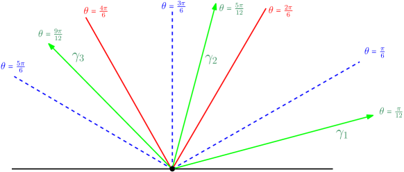
Figure 3: The image of a natural coordinate $\zeta_{k}$ for the monic polynomial differential $q(z)=z^{n}dz^{6}$. In Section 8, we show $\lim_{s\rightarrow\infty}[\nu(\gamma(s))]$ is the same for $\gamma$ any $q$-ray of angle $\theta\in S_{k}:=(\frac{(k-1)\pi}{3},\frac{k\pi}{3})$. The red lines are critical lines, or ‘Stokes lines’, in the sense that the projective limit of $\nu$ along $q$-rays changes as we cross them. The rays $\gamma_{i}$ serve as representative rays for the sector $S_{i}$. The dotted blue lines are ‘Stokes lines’ for $\psi\psi_{0}^{-1}$, but not for $\nu$.

We now note that a version of the construction holds in general for any monic polynomial $q$, as shown by Dumas-Wolf, by treating the general case as a deformation of the model case of a monomial [21]. The essential difference is that the Euclidean rays $\alpha_{k},\alpha_{k-1},\alpha_{k+1}$ are now only eventually contained in $U_{k}$ and moreover these Euclidean rays in the $z$ coordinate become quasi-rays in a natural coordinate $\zeta_{k}$ for $q$. This collection of half-planes will be crucial for the proof of the main theorem, Theorem 8.28.

Lemma 6.4 (Standard Half-Planes (Prop 3.2 [21]) ).

Let $q\in H^{0}(\mathcal{K}_{\mathbb{C}}^{6})$ be a monic polynomial of degree $n$ and $K$ a compact set containing the zeros of $q$. We can find a compact set $K^{\prime}\supset K$ and a set $\{(w_{k},U_{k})\}_{k=1}^{n+6}$ of $q$ half-planes such that

1. $\mathbb{C}-\bigcup_{k=1}^{n+6}U_{k}=K^{\prime}$.

2. The rays $R\left(\frac{2\pi}{n+6}\left(j+\frac{1}{4}\right)\right)$ are eventually contained in $U_{k}$ for $j\in\{k-1,k,k+1\}$.

3. The rays $R\left(\frac{2\pi(k\pm 2)}{n+6}\right)$ are disjoint from $U_{k}$.

4. Euclidean rays are quasi-rays in each $q$-half-plane $(w_{k},U_{k})$. Moreover, $R\left(\frac{2\pi}{n+6}\left(j+\frac{1}{4}\right)\right)$ are $q$-quasi-rays of angles $\frac{\pi}{12},\frac{5\pi}{12},\frac{9\pi}{12}$ for $j=k-1,k,k+1$, respectively.

5. On overlaps $U_{k}\cap U_{k+1}$, we have $w_{k+1}=\zeta^{-1}w_{k}+c$ for $\zeta=e^{\frac{2\pi i}{6}\,}$ and $w_{k},w_{k+1}$ map $U_{k}\cap U_{k+1}$ onto a Euclidean sector of angle $\frac{2\pi}{3}$.

6. Every $q$-ray $\gamma:\mathbb{R}_{+}\rightarrow\mathbb{C}$ is eventually contained in some $U_{i}$.

All of (1) – (5) are explained in the proof from [21], except (6), which we now check. Let $\gamma:\mathbb{R}_{+}\rightarrow\mathbb{C}$ be a $q$-ray. Since $g_{q}:=|q|^{1/3}$ is complete and $\gamma$ is a $g_{q}$-geodesic by definition, $\gamma$ leaves compacta. Thus, for some $s_{0}$, we have $\gamma(s)\in\bigcup_{k=1}^{n+6}U_{j}$ for $s\geq s_{0}$. We claim that for some index $j$, we have $\gamma(s)\in U_{j}$ for $s\geq s_{1}>s_{0}$. To see this, write $\gamma(s_{0})\in U_{i}$. Then let $\theta\in[0,2\pi)$ be the angle of $\gamma$ in $U_{i}$. If $\theta\in(0,\pi)$, we find $\gamma(s)\in U_{i}$ for $s\geq s_{0}$. If $\theta\in[\pi,\frac{4\pi}{3})$, we find $\gamma$ moves into $U_{i+1}$, where it has angle $\theta-\frac{\pi}{3}\in U_{i+1}$ and hence remains in $U_{i+1}$. The argument is similar if $\theta\in(\frac{5\pi}{3},2\pi]$, where $\gamma$ moves into $U_{i-1}$ and remains there. In the final case that $\theta\in[\frac{4\pi}{3},\frac{5\pi}{3}]$, then $\gamma$ travels into an adjacent half-plane $U_{i\pm 1}$ in which it has angle $\theta\pm\frac{\pi}{6}$, reducing to a previous case. We conclude that (6) holds.

Denote $\mathcal{Z}:=q^{-1}(0)$ to be the zeros of $q$ and we define $t:\mathbb{C}\rightarrow\mathbb{R}_{\geq 0}$ by

$$t(p):=\mathsf{dist}_{g_{q}}(p,\mathcal{Z}).$$ (6.1)

Later, we will need $q$-half-planes that have nice asymptotics with respect to this metric $t$.

Proposition 6.5 (Good Asymptotic Half-Planes ([21] Prop A.1) ).

Let $q\in H^{0}(\mathcal{K}_{\mathbb{C}}^{6})$ be a monic polynomial and $K$ a compact set containing the zeros of $q$. Then there are constants $A,R,a>0$ such that for any $p\in\mathbb{C}$ with $t(p)>R$, there is a $q$-half-plane $(w,U)$ with $U\cap K=\emptyset$ and

$$\Im(w(p))>t(p)-A.$$

Moreover, for $x\in\partial U$ in the boundary of this half-plane, we have

$$t(x)>a|\Re(w(x))|\;\;\text{as}\;\;x\rightarrow\infty.$$

6.2 Asymptotics of Decay Term.

In this subsection, we prove the precise a precise asymptotic for the error term $\boldsymbol{\tilde{u}}:=\boldsymbol{u}-\boldsymbol{u}^{-}$ in a natural coordinate for $q$, where $\boldsymbol{u}$ solves (2.25).

We begin with first estimate for the error term $\tilde{\boldsymbol{u}}:=\boldsymbol{u}-\boldsymbol{u}^{-}$, which will be crucial for proving stronger estimates on the the precise rate of decay of $\tilde{\boldsymbol{u}}$.

Corollary 6.6 (A First Estimate).

Let $q\in H^{0}(\mathcal{K}_{\mathbb{C}}^{6})$ be a monic polynomial of degree $n$ and $t:\mathbb{C}\rightarrow\mathbb{R}_{\geq 0}$ be the $|q|^{1/3}$-distance to the zero set of $q$. Then there are constants $C,R,\beta>0$ such that $t(p)>R$, then the complete solution $\boldsymbol{u}=(u_{1},u_{2})$ to equation (2.25) satisfies

$$\begin{cases}\;\;0\leq&u_{1}-\frac{5}{6}\log(\;c|q|\;)<Ct^{-\beta}\\ \;\;0\leq&u_{2}-\frac{1}{6}\log(\;d|q|\;)<Ct^{-\beta},\end{cases}$$ (6.2)

where $\beta=\frac{12\,n}{n+6}>1$.

Proof.

Let $p_{0}:=$ the origin in $\mathbb{C}$ and denote $d_{n}(p):=\mathsf{dist}_{g_{n}}(p,p_{0})$, where $g_{n}:=|z^{\frac{n}{6}}||dz|^{2}$ is the flat metric associated to $q_{n}=z^{n}dz^{6}$.

Using the family of natural $q_{n}$-half-planes from Prop 6.4 of the form $(\zeta_{k},U_{k})$ with $\zeta_{k}=\alpha_{k}\frac{n+6}{6}z^{\frac{n+6}{6}}$, one finds that $d_{n}$ satisfies $d_{n}\asymp\,|p|^{\frac{n+6}{6}}$. Since $q$ and $q_{n}$ are comparable away from the zeros of $q$, for $|z|$ sufficiently large:

$$C_{2}|z|^{n}<|q(z)|<C_{3}|z|^{n}.$$ (6.3)

Similarly, we have $t,d_{n}$ comparable for $|z|$ sufficiently large. In particular, we have

$$t(p)<C_{4}|z|^{\frac{n+6}{6}}.$$ (6.4)

Observe that $0\leq\boldsymbol{u}-\boldsymbol{u}^{-}\leq\boldsymbol{u}^{+}-\boldsymbol{u}^{-}$ by Theorem 5.5. Expanding the right-hand side, we find that for $D_{1}=\frac{5}{12},D_{2}=\frac{1}{12},$

$$u^{+}_{i}-u_{i}^{-}=D_{i}\log\left(1+\frac{A}{|q|^{2}}\right)\leq C_{5}\frac{A}{|q|^{2}}.$$ (6.5)

Combining (6.3), (6.4), we find that for some constants $C^{\prime},C^{\prime\prime}$,

$$|q|^{2}\geq C^{\prime}|z^{2n}|\geq C^{\prime\prime}\,t^{\frac{12n}{n+6}}.$$

Applying this inequality in (6.5) gives the desired inequalities (6.2). ∎

We now write out the new system that the error $\boldsymbol{\tilde{u}}$ solves in a natural coordinate $w$ for $q$. Recall that $\tilde{u}_{1}=u_{1}-\frac{5}{6}\log(c|q|)$ and $\tilde{u}_{2}=u_{2}-\frac{1}{6}\log(d|q|)$. In $w$ coordinates, $\tilde{u}_{1}(w)=u_{1}(w)-\log(c^{5/6})$ and $\tilde{u}_{2}=u_{2}-\log(d^{1/6})$. Since $\Delta\equiv\Delta_{g_{q}}$ in $w$-coordinates, for $b=\frac{6d^{1/3}}{2}$ from earlier, we find $\boldsymbol{\tilde{u}}$ solves

$$\begin{cases}\Delta\tilde{u}_{1}&=b\left(\,e^{\tilde{u}_{1}-3\tilde{u}_{2}}-\,e^{-2\tilde{u}_{1}}\right)\\ \Delta\tilde{u}_{2}&=b\left(e^{2\tilde{u}_{2}}-e^{\tilde{u}_{1}-3\tilde{u}_{2}}\right).\end{cases}$$ (6.6)

The linearization of the system (6.6) at zero is

$$\begin{cases}\Delta\tilde{u}_{1}&=b(3\tilde{u}_{1}-3\tilde{u}_{2})\\ \Delta\tilde{u}_{2}&=b(5\tilde{u}_{2}-\tilde{u}_{1})\end{cases}$$ (6.7)

Set $x_{1}=\tilde{u}_{1}+\tilde{u}_{2}$ and $x_{2}=\tilde{u}_{1}-3\tilde{u}_{2}$. Then $x_{1},x_{2}$ are eigenvectors of the linearized system (6.7), with eigenvalues $2b,6b$, respectively. We are led to recall some results on the growth rate of solutions to $\Delta u=ku$ with prescribed boundary values.

Lemma 6.7 (Classical Estimates (Lemma 5.8 [21])).

Let $0\leq g\in C^{0}(\mathbb{R})\cap L^{1}(\mathbb{R})$ and $k>0$. Then the boundary value problem

$$\begin{cases}\Delta h&=kh\\ h|_{\mathbb{R}}&=g\end{cases}$$

has a solution $h\in C^{\infty}(\mathbb{H})\cap C^{0}(\mathbb{R})$ with $0\leq h\leq g$. Moreover, in the standard $z=x+iy$ coordinate,

$$h\in O\left(\frac{e^{-2\sqrt{k}y}}{y}\,\right)\;\;\text{as}\;\;y\rightarrow\infty.$$

We now discuss super-solutions to a quadratic version of the same equation.

Lemma 6.8 (Quadratic Super-solution ([58] Lemma 3.13)).

Let $g\in C^{0}(\mathbb{R})\cap L^{1}(\mathbb{R})$ with a global bound $0\leq g\leq\frac{1}{4k^{\prime}}$ and $k>0$. Then there is a smooth super-solution $v\in C^{\infty}(\mathbb{H})\cap C^{0}(\mathbb{R})$ satisfying, for $z=x+iy$ on $\mathbb{H}$,

$$\begin{cases}\Delta v\leq kv-kk^{\prime}v^{2}\\ v|_{\mathbb{R}}\geq g\end{cases}$$

as well as

$$v\in O\left(\frac{e^{-2\sqrt{k}y}}{\sqrt{y}}\right)\;\;\text{as}\;\;y\rightarrow\infty.$$

We can now show the precise asymptotics of the error terms $x_{1},x_{2}$, using both Lemmas 6.7 and 6.8. It is essential to the proof that the error $\tilde{\boldsymbol{u}}$ is a priori integrable; for this fact we need Prop 6.6.

Lemma 6.9 (Fundamental Asymptotics).

Let $q\in H^{0}(\mathcal{K}_{\mathbb{C}}^{6})$ be a polynomial and $t:\mathbb{C}\rightarrow\mathbb{R}_{\geq 0}$ be the distance from the zeros of $q$. Then for $\alpha=2^{1/3}3^{1/4}5^{1/3}$, as $t\rightarrow\infty$,

$$x_{1}\in O\left(\,\frac{e^{-2\alpha\,t}}{\sqrt{t}}\,\right)\;\;\;\text{and}\;\;\;x_{2}\in O\left(\,\frac{e^{-2\alpha\sqrt{3}\,t}}{\sqrt{t}}\,\right).$$

Moreover, $\Delta x_{i}\in O(x_{i})$ satisfies the same asymptotics as $x_{i}$.

Proof.

Recall by Corollary 6.6, that $\tilde{u}_{i}$ are uniformly bounded away from the zeros of $q$. Thus, we select a compact set $K$ containing the zeros of $q$ such that

$$0\leq\tilde{u}_{i}\leq\frac{1}{16}\;\text{on}\;\mathbb{C}-K.$$ (6.8)

By iteratively applying Proposition 6.5, we may take a collection $\{(w_{k},U_{k})\}_{k=1}^{N}$ of $q$-half-planes covering $\{p\in\mathbb{C}\;:\;t(p)>R\}$, for $R$ sufficiently large, such that the $t$-asymptotics of Prop 6.5 hold. It suffices to prove the asymptotics in each half-plane $(w_{k},U_{k})$. Fix a $q$-half-plane $(w_{k},U_{k})$ and identify $\mathbb{H}=U_{k}$ and $\mathbb{R}=\partial\mathbb{H}=\partial U_{k}$. We write $w=w_{k}$ for notational simplicity and set $w=x+iy$. In these coordinates, $\tilde{u}_{1},\tilde{u}_{2}$ satisfy the system (6.6) and $\tilde{u}_{i}\geq 0$.

We first show the asymptotic for $x_{1}=\tilde{u}_{1}+\tilde{u}_{2}$. By direct calculation, $x_{1}$ satisfies

$$\Delta x_{1}=be^{2\tilde{u}_{2}}-be^{-2\tilde{u}_{1}}.$$ (6.9)

Since $\tilde{u}_{i}\geq 0$, we have $e^{2\tilde{u}_{2}}\geq 1+2\tilde{u}_{2}+2\tilde{u}_{2}^{2}$ and $e^{-2\tilde{u}_{1}}\leq 1-2\tilde{u}_{1}+2\tilde{u}_{1}^{2}$. Combining these inequalities,

$$\Delta x_{1}\geq 2b\,x_{1}-2b\,(\tilde{u}_{1}^{2}-\tilde{u}_{2}^{2})\geq 2b\,x_{1}-2b\,x_{1}^{2}.$$ (6.10)

Since $x_{1}\geq 0$, we see $g_{1}:=x_{1}|_{\mathbb{R}}$ is non-negative and continuous too. By Corollary 6.6, $x_{1}\in O(t^{-\beta})$ for $\beta>1$, for $p$ sufficiently large. Also, for $p\in\mathbb{R}$ sufficiently large, $t(p)>a|\Re(w(p))|$, for some $a>0$, by Proposition 6.5. We conclude that $g_{1}\in L^{1}(\mathbb{R})$ is integrable. The bounds (6.8) on $\tilde{u}_{i}$ imply $g_{1}\leq\frac{1}{4}$. We note here that $\sqrt{2b}=\sqrt{6d^{1/3}}=\alpha$. Hence, we may apply Lemma 6.8 with $k=2b$ and $k^{\prime}=1$ to get a function $v$ satisfying $v\in O\left(\frac{e^{-2\alpha\,y}}{\sqrt{y}}\right)$ as well as

$$\begin{cases}\Delta v\leq 2b\,v-2b\,v^{2}\\ v|_{\mathbb{R}}\geq g_{1}\end{cases}.$$ (6.11)

Next, recall the uniform inequality $t\leq y+A$ from Proposition 6.5 part (ii), for $t$ sufficiently large, for some $A>0$. This inequality implies $v\in O\left(\frac{e^{-2\alpha t}}{\sqrt{t}}\right)$. Thus, it suffices to show $\eta=x_{1}-v\leq 0$.

By (6.11), $\eta\leq 0$ on $\mathbb{R}$ and $\eta\rightarrow 0$ as $|w|\rightarrow\infty$. Suppose $\eta>0$ somewhere. Then for some $\epsilon>0$, there is a $q\in\mathbb{H}$ with $\eta(q)>\epsilon$. Since $\eta\rightarrow 0$, we find $Q=\eta^{-1}(\,[\epsilon,\infty)\,)$ is a compact region. Thus, $\eta$ attains a maximum at some point $p\in Q$. Hence, $\Delta\eta(p)\leq 0$. On the other hand,

$$\Delta\eta=\Delta x_{1}-\Delta v=2b\,x_{1}-2b\,x_{1}^{2}-2b\,v+2bv^{2}\geq 2b\,\eta-2b\,(x_{1}^{2}-v^{2})=2b\,\eta-2b\,\eta(x_{1}+v).$$ (6.12)

Now, $\eta(p)>\epsilon>0$ implies $v(p)<x_{1}(p)$. Hence, $v(p)+x_{1}(p)<\frac{1}{2}$ by (6.8). Evaluating at $p$, we find

$$0\geq\Delta\eta(p)\geq b\,\eta(p)>0,$$

a contradiction. We conclude that $\eta\leq 0$ as desired, finishing the proof of the asymptotic for $x_{1}$.

We must be more careful with $x_{2}=\tilde{u}_{1}-3\tilde{u}_{2}$, as it may not be non-negative, but we can now leverage the asymptotic for $x_{1}$. We work in the same $q$-half-plane $(w,U)$ as before. Set $x_{2}^{\prime}:=|x_{2}|$. Then the global bounds (6.8) now give $0\leq x_{2}^{\prime}\leq\frac{1}{2}$ on $\mathbb{H}$. By direct calculation with (6.6), $x_{2}$ satisfies

$$\Delta x_{2}=4b\,e^{x_{2}}-b\,e^{-2\tilde{u}_{1}}-3b\,e^{2\tilde{u}_{2}}.$$ (6.13)

We now proceed in cases by sign. Suppose $x_{2}(p)\geq 0$ at some point $p\in\mathbb{H}$. Then we apply the global inequalities (i) $e^{x_{2}}\geq 1+x_{2}$   (ii) $e^{-2\tilde{u}_{1}}\leq 1-2\tilde{u}_{1}+2\tilde{u}_{1}^{2}$ as well as (iii) $e^{2\tilde{u}_{2}}\leq 1+2\tilde{u}_{2}+2\tilde{u}_{2}^{2}$, which holds for $t$ sufficiently large since $\tilde{u}_{2}\rightarrow 0$. Applying (i) - (iii) in (6.13), if is $t$ sufficiently large and $x_{2}(p)\geq 0$,

$$\Delta x_{2}\geq 6b\,x_{2}-2b\,\tilde{u}_{1}^{2}-6b\,\tilde{u}_{2}^{2}\geq 6b\,x_{2}-6b\,x_{1}^{2}.$$ (6.14)

Suppose instead $x_{2}(p)<0$. Then $e^{x_{2}(p)}\leq 1+x_{2}(p)+\frac{1}{2}x_{2}^{2}(p)$. We can also apply the (global) inequalities $e^{-2\tilde{u}_{1}}\geq 1-2\tilde{u}_{1}$ and $e^{2\tilde{u}_{2}}\geq 1+2\tilde{u}_{2}$ in (6.13). Finally, with $x_{2}^{2}\leq 9x_{1}^{2}$, we find that for $x_{2}(p)<0$,

$$\Delta(-x_{2})\geq 6b\,(-x_{2})-2b\,x_{2}^{2}\geq 6b\,(-x_{2})-18b\,x_{1}^{2}.$$ (6.15)

Combining (6.14), (6.15), we have $\Delta x_{2}^{\prime}\geq 6b\,x_{2}^{\prime}-18b\,x_{1}^{2}$ for $t$ large. The first part of the proof implies $x_{1}^{2}\in O\left(\frac{e^{-4\alpha\,t}}{t}\right)$. Set $g_{2}:=x_{2}^{\prime}|_{\mathbb{R}}$ and $0\leq g_{2}\leq\frac{1}{2}$ from $\tilde{u}_{i}\leq\frac{1}{8}$. As before, $g_{2}$ is integrable from Corollary 6.6 and Proposition 6.5. We observe that $x_{2}^{\prime}$ is a sub-solution to the boundary value problem (6.16) on the complement of a compact set.

$$\begin{cases}\Delta h=6b\,h-18b\,x_{1}^{2}.\\ h|_{\mathbb{R}}=g_{2}.\end{cases}$$ (6.16)

To finish the proof, we must show $x_{2}^{\prime}\in O\left(\,\frac{e^{-2\alpha\sqrt{3}\,t}}{\sqrt{t}}\right)$. To this end, we construct a super-solution $h\in C^{\infty}(\mathbb{H})$ in Lemma 6.11 to (6.16) that satisfies the desired asymptotic. The maximum principle shows $x_{2}^{\prime}\leq h$ holds on the domain of $h$, as earlier in the proof with $\eta$, which proves the asymptotic for $x_{2}^{\prime}$.

For the final claim on $\Delta x_{i}$, we recall that $x_{i}$ are each eigenvectors of the linearized systems. In particular, $\Delta x_{i}=C_{i}x_{i}+O(x_{i}^{2})$. We conclude that $\Delta x_{i}$ satisfies the same $t$-asymptotics as $x_{i}$. ∎

We note as a corollary that $\partial x_{i}$ has the same asymptotics as $x_{i}$.

Corollary 6.10.

Under the same hypotheses as Lemma 6.9, we have

$$\partial x_{1}\in O\left(\,\frac{e^{-2\alpha\,t}}{\sqrt{t}}\,\right)\;\;\;\text{and}\;\;\;\partial x_{2}\in O\left(\,\frac{e^{-2\alpha\sqrt{3}\,t}}{\sqrt{t}}\,\right).$$

Proof.

We first note that that $\Delta(x_{i})\in O(x_{i})$ by the fact that $x_{i}$ are eigenvectors of the linearized system and $x_{i}$ decays exponentially. Applying the interior estimate for the gradient (c.f. Theorem 3.9 [30] ) to $x_{i}$ on a ball of radius 1 around a point $p_{0}$ of distance $t$ from the zeros of $q$ gives the desired result by Lemma 6.9. ∎

Lemma 6.11.

Let $g\in C^{0}(\mathbb{R})\cap L^{1}(\mathbb{R})$ with $0\leq g\leq 1$. Let $t$ denote the $|q|^{1/3}$ distance from the zeros of $q$ and take $f\in O\left(\frac{e^{-4\alpha t}}{t}\right)$ as $t\rightarrow\infty$. Then there is a super-solution $u\in C^{\infty}(\mathbb{H})\cap C^{0}(\mathbb{R})$ satisfying

$$\begin{cases}\Delta u\leq 6b\,u-f.\\ u|_{\mathbb{R}}\geq g,\end{cases}$$

Moreover, as $t\rightarrow\infty,$ for $\alpha=2^{1/3}3^{1/4}5^{1/3}$, we have

$$u\in O\left(\frac{e^{-2\sqrt{3}\alpha\,t}}{\sqrt{t}}\right).$$

Proof.

First, select $h$ from Lemma 6.7 with respect to $k=6b$ and the same $g$ as its boundary values. Then $h\in O\left(\frac{e^{-2\sqrt{3}\alpha\,t}}{\sqrt{t}}\right)$ since $2\sqrt{6b}=2\sqrt{3}\alpha$, using again the argument from Lemma 6.9 to replace $y$ with $t$. We will construct our desired super-solution by $u=2h-h^{\beta}$ for $1<\beta<\frac{2}{\sqrt{3}}$. First, note that since $g\leq 1$ and $\beta>1$, we have $u|_{\mathbb{R}}=2g-g^{\beta}\geq g$. We need only show $\Delta u-6b\,u+f\leq 0$ to finish the proof.

By an elementary calculation, $\Delta(h^{\beta})=\beta(\beta-1)h^{\beta-2}|\nabla h|^{2}+\beta h^{\beta-1}\Delta h$. Since $\Delta h=6b\,h$ by construction of $h$, we get the inequality

$$\Delta(h^{\beta})\geq 6b\beta\,h^{\beta}.$$ (6.17)

By definition of $u$, (6.17) implies the inequality $\Delta u\leq 12b\,h-6b\beta\,h^{\beta}.$ It follows that

$$\Delta u-6b\,u+f\leq 6bh^{\beta}\,(1-\beta)+f.$$

Since $h\in O\left(\frac{e^{-2\sqrt{3}t}}{\sqrt{t}}\right)$, we see that $f\in o(h^{\beta})$ for chosen $\beta$. Set $C=6b(1-\beta)<0$. Then for $R$ sufficiently large, $t>R$ implies $f<-\frac{C}{2}h^{\beta}$ and hence $\Delta u-6b\,u+f<0$. ∎

Remark 6.12.

Let $(w,U)$ be a natural $q$-half-plane. We observe that the same asymptotics for $x_{1},x_{2}$ from Lemma 6.9 hold in the $w$-coordinate, when $t$ is replaced with the Euclidean distance from the origin in $\mathbb{H}$, denoted $r$. Indeed, there are constants $c,C$ such that $t(p)-c\leq r(w(p))\leq t(p)+C$.

7 Asymptotic Parallel Transport & Unipotent Transitions

In this section, we use the precise rate of exponential decay of the error term $\boldsymbol{\tilde{u}}=\boldsymbol{u}-\boldsymbol{u}^{-}$ to compute the asymptotic parallel translation $\mathcal{P}_{z}:\mathcal{E}_{z}\rightarrow\mathcal{E}_{0}$ in the bundle $\mathcal{E}$. We calculate the limit of $\mathcal{P}_{z}$ in a natural coordinate for $q$ along quasi-rays. In particular, we find that the limits $\mathcal{P}_{\theta}:=\lim_{t\rightarrow\infty}\mathcal{P}_{\gamma_{\theta}(t)}$ of the parallel translation along Euclidean rays (or quasi-rays) $\gamma_{\theta}(t)=te^{i\theta}$ of angle $\theta$ are constant for angles $\theta\in I_{k}$ for certain intervals $I_{k}$. We call these limits $\mathcal{P}_{\theta}$, for $\theta\in I_{k}$, stable limits. Moreover, when crossing certain exceptional angles $\theta\in\mathcal{U}$ for some finite set $\mathcal{U}$, we see the stable limits change. We call these angles $\theta\in\mathcal{U}$ unstable. Finally, we relate the neighboring stable limits $\mathcal{P}_{\theta-\epsilon},\mathcal{P}_{\theta+\epsilon}$ reached by crossing a ray in the direction of an unstable angle $\theta\in\mathcal{U}$. In particular, the transition between the stable limits is given by a unipotent matrix, computed in Lemma 7.3.

The ODE for Parallel Translation. We now write the ODE for the matrix representative of $\nabla$-parallel translation. We fix the origin $p_{0}$ as a distinguished basepoint in $\mathbb{C}$. Formally, we view a frame $\mathcal{F}$ as a section $\mathcal{F}\in\Gamma(\;\mathsf{Hom}_{\mathbb{C}}(\uline{\mathbb{C}}^{7},\mathcal{E})\,)$. We equip $\mathsf{Hom}_{\mathbb{C}}(\uline{\mathbb{C}}^{7},\mathcal{E})$ with the product connection, where $\mathcal{E}$ is equipped with $\nabla$ and $\uline{\mathbb{C}}^{7}$ with $d$. We write $(\textbf{e}_{i})_{i=3}^{-3}$ as the standard frame in $\uline{\mathbb{C}}^{7}$, indexed to match the powers of $\mathcal{K}$ in $\mathcal{E}$. We define the standard frame $\mathcal{F}=(f_{i})_{i=3}^{-3}$ by

$$f_{i}:=\textbf{e}_{i}\mapsto u_{i}$$ (7.1)

for $\mathcal{B}=(u_{i})_{i=3}^{-3}$ from (2.14).

Define $\widetilde{\mathcal{F}}_{z}$ as the $\nabla$-parallel translation of $\mathcal{F}_{p_{0}}$ to the fiber $\mathcal{E}_{z}$. We search for the endomorphism $\psi\in\mathsf{End}(\uline{\mathbb{C}}^{7})$ satisfying $\widetilde{\mathcal{F}}\psi=\mathcal{F}$, i.e., expressing the change of basis from $\widetilde{\mathcal{F}}$ to $\mathcal{F}$. Equivalently, $\psi=[\mathcal{P}_{z}:\mathcal{E}_{z}\rightarrow\mathcal{E}_{p_{0}}]$ is the matrix representation of parallel translation in the standard frame $\mathcal{F}$. We now compute the ODE satisfied by $\psi$ along a Euclidean ray $\gamma(t)=te^{i\theta}$ for $t\geq 0$. We use the shorthand $\mathcal{F}(t):=\mathcal{F}(\gamma(t))$ going forward.

On the one hand, the product rule and the fact that $\widetilde{\mathcal{F}}$ is $\nabla$-parallel yields

$$\nabla_{\frac{\partial}{\partial t}}\mathcal{F}(t)=\nabla_{\frac{\partial}{\partial t}}(\widetilde{\mathcal{F}}\psi)(t)=\left(\widetilde{\mathcal{F}}\frac{d\psi}{dt}\right)(t).$$

Conversely, since $\mathcal{F}=\mathsf{id}$ in the basis $\mathcal{B}$,

$$\nabla_{\frac{\partial}{\partial t}}\mathcal{F}(t)=\mathcal{F}\mathcal{A}(e^{i\theta})=\widetilde{\mathcal{F}}\psi(t)(\,e^{i\theta}(\varphi+D_{H})+e^{-i\theta}\varphi^{*}\,).$$

Combining these equations, we deduce that $\psi(t)$ solves the following initial value problem.

$$\begin{cases}\psi^{-1}\frac{d\psi}{dt}&=\,(\varphi+D_{H})e^{i\theta}+\varphi^{*}e^{-i\theta}\\ \psi(0)&=\mathsf{id},\end{cases}$$ (7.2)

where $D_{H}=\nabla_{\overline{\partial},h}^{1,0}=H^{-1}\partial H$.

7.1 Parallel Translation when $q=1$.

In this section, we compute the $\nabla$-parallel translation endomorphism $\psi_{0}$ explicitly when $q_{0}\equiv 1$. In the next section, we show the parallel translation endomorphism $\psi$ for general monic polynomial $q$ is asymptotic to $\psi_{0}$ in a natural coordinate for $q$.

Observe that when $q_{0}=dz^{6}$, the solution to Hitchin’s equations (2.24) is $\log(r^{2}s)=\log(c^{5/3}),\log(s)=\log(d^{1/3})$, by the equation (5.3), which is now a global solution. Using the relations (2.26), we find

$$r_{0} =\frac{6}{5}d^{2/3}=\left(\frac{2}{5}\right)^{1/3}$$ (7.3)

$$s_{0} =d^{1/3}=\frac{1}{\sqrt{3}}\left(\frac{5}{2}\right)^{1/3}.$$ (7.4)

Thus, the matrix representative of the harmonic metric $h_{0}$ is given by

$$H_{0}=\mathsf{diag}\,\left(\,\sqrt{3},\,\left(\frac{5}{2}\right)^{1/3},\,\sqrt{3}\left(\frac{2}{5}\right)^{1/3},\,1,\,\frac{1}{\sqrt{3}}\left(\frac{5}{2}\right)^{1/3},\,\left(\frac{2}{5}\right)^{1/3},\frac{1}{\sqrt{3}}\right).$$ (7.5)

We now solve explicitly for the parallel translation matrix $\psi_{0}$ from (7.2). The constant case is exceptional, since $\varphi,\varphi^{*h}$ commute. Since the Higgs field $\varphi_{0}$ and its adjoint $\varphi_{0}^{*}$ are constant matrices in the standard coordinates, we find $\psi_{0}(z)=e^{z\varphi_{0}+\bar{z}\varphi^{*}_{0}}$ solves the initial value problem (7.2).

Let us simultaneously diagonalize $\varphi_{0},\varphi^{*}_{0}$. The mutual eigenvalues are recorded in the diagonal matrix

$$D=\mathsf{diag}(\alpha\xi^{1},\alpha\xi^{3},\alpha\xi^{5},\alpha\xi^{7},\alpha\xi^{9},\alpha\xi^{11},0),$$ (7.6)

where $\xi=e^{\frac{\pi i}{6}}$ and

$$\alpha=5^{1/6}3^{1/4}2^{1/3}.$$ (7.7)

The corresponding eigenvectors recorded as a matrix $E_{0}$. We also obtain

$$\varphi_{0} =E_{0}DE_{0}^{-1}$$ (7.8)

$$\varphi_{0}^{*} =E_{0}\overline{D}E_{0}^{-1}.$$ (7.9)

Using the identity $e^{gGg^{-1}}=ge^{G}g^{-1}$, one finds

$$\psi_{0}=E_{0}e^{zD+\overline{zD}}E_{0}^{-1}=E_{0}e^{2\,\mathrm{Re}(zD)}E_{0}^{-1}.$$

We can explicitly describe the eigenvector matrix $E_{0}$ by factoring it. To this end, set

$$(H_{0})^{-1/2} =\mathsf{diag}\left(\;3^{-\frac{1}{4}},\;\frac{2^{1/6}}{5^{1/6}},\;\frac{5^{1/6}}{3^{\frac{1}{4}}2^{1/6}},\;1,\;\frac{3^{1/4}2^{1/6}}{5^{1/6}},\;\frac{5^{1/6}}{2^{1/6}}\;3^{\frac{1}{4}}\right)$$ (7.10)

$$S =\frac{1}{\sqrt{6}}\begin{pmatrix}\frac{1}{\sqrt{2}}&\frac{1}{\sqrt{2}}&\frac{1}{\sqrt{2}}&\frac{1}{\sqrt{2}}&\frac{1}{\sqrt{2}}&\frac{1}{\sqrt{2}}&\sqrt{-3}\\ \xi^{11}&\xi^{9}&\xi^{7}&\xi^{5}&\xi^{3}&\xi&0\\ \xi^{10}&-1&\xi^{2}&\xi^{10}&-1&\xi^{2}&0\\ -1&1&-1&1&-1&1&0\\ \xi^{2}&-1&\xi^{10}&\xi^{2}&-1&\xi^{10}&0\\ \xi&\xi^{3}&\xi^{5}&\xi^{7}&\xi^{9}&\xi^{11}&0\\ \frac{1}{\sqrt{2}}&\frac{1}{\sqrt{2}}&\frac{1}{\sqrt{2}}&\frac{1}{\sqrt{2}}&\frac{1}{\sqrt{2}}&\frac{1}{\sqrt{2}}&-\sqrt{-3}\end{pmatrix}.$$ (7.11)

A (computer-assisted) calculation shows the matrix $E_{0}$ is an eigenvector matrix for $\varphi_{0}$ satisfying (7.8), where

$$E_{0}=H_{0}^{-1/2}S.$$ (7.12)

We switch now to polar coordinates $z=re^{i\theta}$ and set $\mathcal{D}=e^{2\,\Re(zD)}$ so that

$$\psi_{0}=E_{0}\mathcal{D}E_{0}^{-1}.$$ (7.13)

Here,

$$\mathcal{D}=\mathsf{diag}(e^{2\alpha r\,\cos(\theta+\frac{\pi}{6})},e^{2\alpha r\,\cos(\theta+\frac{3\pi}{6})},e^{2\alpha r\,\cos(\theta+\frac{5\pi}{6})},e^{2\alpha r\,\cos(\theta+\frac{7\pi}{6})},e^{2\alpha r\,\cos(\theta+\frac{9\pi}{6})},e^{2\alpha r\,\cos(\theta+\frac{11\pi}{6})},1).$$ (7.14)

We also write

$$\mathcal{D}=e^{2\alpha r\,\mathscr{D}},$$ (7.15)

where $\mathscr{D}=\mathsf{diag}(d_{i})_{i=1}^{7}$ is given by $d_{i}=\frac{1}{|z|}\,\Re(\xi^{2i+1}z)$ for $i\in\{1,2,3,4,5,6\}$ and $d_{7}=0$:

$$\mathscr{D}=\mathsf{diag}\left(\cos\left(\theta+\frac{\pi}{6}\right),\;\cos\left(\theta+\frac{3\pi}{6}\right),\;\cos\left(\theta+\frac{5\pi}{6}\right),\;\cos\left(\theta+\frac{7\pi}{6}\right),\;\cos\left(\theta+\frac{9\pi}{6}\right),\cos\left(\theta+\frac{11\pi}{6}\right),\;0\right).$$ (7.16)

The global bounds of $d_{i}$ on the intervals $I_{k}:=(\frac{(k-1)\pi}{6},\frac{k\pi}{6})\subset\mathbb{R}$ will be crucial for computing the asymptotic $\nabla$-parallel translation in the general case. We will use $d_{j+3}=-d_{j}$ repeatedly. We note that for $j\in\mathbb{Z}_{6}$, we have the following bounds:

$$\;\;\;\;\;\;\;\text{for}\;\theta\in I_{k},\;\;|d_{i}(\theta)-d_{j}(\theta)|<\begin{cases}1&|i-j|=1,5\mod 6\\ \sqrt{3}&|i-j|=2,4\mod 6\\ 1&i=7\;\text{or}\;j=7\end{cases}$$ (7.17)

The case of $i=7$ or $j=7$ is clear since $d_{7}=0$. Hence, it suffices to prove the cases $j=1,2\mod 6$. We omit the argument by elementary calculus to show that these inequalities are, in fact, strict in each sector.

7.2 Asymptotic Parallel Translation

We now return to our parallel translation endomorphism $\psi$ solving (7.2) and satisfying $\widetilde{\mathcal{F}}\psi=\mathcal{F}$. We show the solution $\psi$ with respect to monic polynomial $q$ is asymptotic to $\psi_{0}$, the solution when $q\equiv 1$, along certain sectors of of a natural coordinate $(w,U)$ for $q$. The asymptotics for $\psi$ are a consequence of the asymptotics of the error term from Section 6.

We now derive a new ODE for $B:=\psi\psi_{0}^{-1}$ along a ray $\gamma(s)=se^{i\theta}$ in a $q$-half-plane $(w,U)$. We aim to show the limit of $B$ exists along stable rays, as defined shortly. We now recall that that $\psi(t)=\psi(\gamma(s))$ and $\psi_{0}(s)=\psi_{0}(\gamma(s))$ satisfy the following initial value problems for some $A,A_{0}\in\mathsf{G}_{2}$:

$$\begin{cases}&\psi^{-1}\frac{d\psi}{ds}=e^{i\theta}(D_{H}+\varphi)+e^{-i\theta}\varphi^{*}\\ &\psi(s_{0})=A\end{cases}\;\;\text{and}\;\;\begin{cases}&\psi_{0}^{-1}\frac{d\psi_{0}}{ds}=e^{i\theta}\varphi_{0}+e^{-i\theta}\varphi^{*}_{0}\\ &\psi_{0}(s_{0})=A_{0}.\end{cases}.$$

By an elementary calculation, $B(t):=\psi\psi_{0}^{-1}(\gamma(t))$ is a solution to the initial value problem

$$\begin{cases}B^{-1}dB=\psi_{0}\,R\,\psi_{0}^{-1}\\ B(0)=A_{0}^{-1}A_{0}\end{cases},$$

where the error term $R$ is given by

$$R=\psi^{-1}d\psi-\psi_{0}^{-1}d\psi_{0}.$$ (7.18)

Since $\varphi\equiv\varphi_{0}$ in a natural coordinate for $q$, we conclude that

$$B^{-1}\frac{dB}{ds}=\psi_{0}\,\left(e^{i\theta}D_{H}+e^{-i\theta}(\varphi^{*}-\varphi^{*}_{0})\,\right)\,\psi_{0}^{-1}.$$ (7.19)

We denote

$$\Theta:=B^{-1}dB=\psi_{0}\,R\,\psi_{0}^{-1}.$$

The asymptotic analysis of $\Theta$ going forward involves a comparison of the exponential growth of $\psi_{0}$ in these coordinates to the exponential decay of the matrix $R$.

We now split the error matrix $R=e^{i\theta}D_{H}+e^{-i\theta}(\varphi^{*}-\varphi^{*}_{0})$ into two terms

$$R^{\prime} =e^{i\theta}D_{H}$$ (7.20)

$$R^{\prime\prime} =e^{-i\theta}(\varphi^{*}-\varphi^{*}_{0}).$$ (7.21)

Recalling the expression (7.13) for $\psi_{0}$, we re-write $\Theta$ once more as

$$\Theta=E_{0}(\mathcal{D}(R_{1}+R_{2})\mathcal{D}^{-1})E_{0}^{-1},$$ (7.22)

where

$$R_{1}: =E_{0}^{-1}R^{\prime}E_{0}=S^{-1}R^{\prime}S$$ (7.23)

$$R_{2}: =E_{0}^{-1}R^{\prime\prime}E_{0}.$$ (7.24)

The first equation follows from the expression $E_{0}=H_{0}^{-1/2}S$ for $E_{0}$ and the fact that $H_{0}^{1/2}$ and $R^{\prime}$ commute. Since $E$ is a constant-coefficient matrix, the asymptotics of $\Theta$ depend only on $\text{Ad}_{\mathcal{D}}(R_{i})$. Using the expression (7.15) for $\mathcal{D}$, we observe that as we conjugate the error matrix $R_{k}$ by $\mathcal{D}$, the $(i,j)$ entry of $R_{k}$ is multiplied by $e^{2\alpha\,s(d_{i}-d_{j})}$. By the bounds (7.17), we have upper bounds on the exponent of $e^{2\alpha\,s(d_{i}-d_{j})(\theta)}$ for $\theta\in I_{k}$. We now determine the precise rate of decay of $(R_{k})_{ij}$.

Recall that $r=e^{u_{1}-u_{2}},s=e^{2u_{2}}$. Since $u_{i},\tilde{u}_{i}$ differ only by constants, we find $R^{\prime},R^{\prime\prime}$ are given by

$$R^{\prime} =\begin{pmatrix}-\partial(\tilde{u}_{1}+\tilde{u}_{2})&&&&&&\\ &-\partial(\tilde{u}_{1}-\tilde{u}_{2})&&&&&\\ &&-2\,\partial\tilde{u}_{2}&&&&\\ &&&0&&&\\ &&&&2\,\partial\tilde{u}_{2}&&\\ &&&&&\partial(\tilde{u}_{1}-\tilde{u}_{2})&\\ &&&&&&\partial(\tilde{u}_{1}+\tilde{u}_{2})\\ \end{pmatrix}$$ (7.25)

$$R^{\prime\prime} =\begin{pmatrix}0&\sqrt{3}\,(s-s_{0})&&&&&\\ &0&\sqrt{5}(\frac{r}{s}-\frac{r_{0}}{s_{0}})&&&&\\ &&0&\sqrt{-6}(s-s_{0})&&&\\ &&&0&\sqrt{-6}(s-s_{0})&&\\ &&&&0&\sqrt{5}(\frac{r}{s}-\frac{r_{0}}{s_{0}})&\\ \frac{1}{r^{2}s}-\frac{1}{r_{0}^{2}s_{0}}&&&&&0&\sqrt{3}\,(s-s_{0})\\ &\frac{1}{r^{2}s}-\frac{1}{r_{0}^{2}s_{0}}&&&&&0\\ \end{pmatrix}.$$ (7.26)

Now, by (computer-assisted) matrix multiplication, we find that the entries of $R_{1}=E_{0}^{-1}R^{\prime}E_{0}$,  $R_{2}=E_{0}^{-1}R^{\prime\prime}E_{0}$ are scalar multiples of $x_{1}=\tilde{u}_{1}+\tilde{u}_{2},\,x_{2}=\tilde{u}_{1}-3\tilde{u}_{2}$ and their derivatives. In particular, we have a combinatorial description of the entries of $R_{1}$ as follows:

$$(R_{1})_{ij}=\begin{cases}\asymp(\partial x_{1})&|i-j|=1,5\mod 6\\ \asymp(\partial x_{2})&|i-j|=2,4\mod 6\\ 0&|i-j|=0,3\mod 6\\ \asymp(\,(1-\delta_{ij})\partial x_{1})&i=7\;\text{or}\;j=7.\end{cases}$$ (7.27)

Here, $\asymp$ denotes asymptotically comparable. That is, $f(s)\asymp g(s)$ when there exist constants $c,C$ such that $c|g(s)|\,\leq|f(s)|\leq\,C|g(s)|$ for $s$ sufficiently large.

We work a little harder for the analogous description of $R_{2}$. First, we observe the following:

$$s-s_{0} =d^{1/3}(e^{2\tilde{u}_{2}}-1)=2d^{1/3}\tilde{u}_{2}+O(x_{1}^{2})$$ (7.28)

$$\frac{1}{r^{2}s}-\frac{1}{r_{0}^{2}s_{0}} =c^{-5/3}(e^{-2\tilde{u}_{1}}-1)=-2c^{-5/3}\tilde{u}_{1}+O(x_{1}^{2})$$ (7.29)

$$\frac{r}{s}-\frac{r_{0}}{s_{0}} =c^{5/6}d^{-1/2}(e^{\tilde{u}_{1}-3\tilde{u}_{2}}-1)=c^{5/6}d^{-1/2}x_{2}+O(x_{2}^{2}).$$ (7.30)

Combining the asymptotics (7.28) – (7.30) with equation (7.26), again a (computer-assisted) matrix multiplication shows $R_{2}=E_{0}^{-1}R^{\prime\prime}E_{0}$ admits a similar asymptotic description to that of $R_{1}$. Indeed,

$$(R_{2})_{ij}=\begin{cases}\asymp(x_{1})&|i-j|=1,5\mod 6\\ \asymp(x_{2})&|i-j|=2,4\mod 6\\ 0&|i-j|=0,3\mod 6\\ \asymp((1-\delta_{ij})\,x_{1})&i=7\;\text{or}\;j=7.\end{cases}$$ (7.31)

We can now prove the existence of the limit $\psi\psi_{0}^{-1}$ along stable rays or quasi-rays in a natural coordinate. We discuss the appropriate notion of stability here.

Definition 7.1.

Let $\gamma(t)=te^{i\theta}$ be a ray in a standard $q$-half-plane. We call $\gamma$ stable when $\theta\notin\{0,\frac{\pi}{6},\frac{2\pi}{6},\frac{3\pi}{6},\frac{4\pi}{6},\frac{5\pi}{6},\pi\}$. We call a quasi-ray $\gamma^{\prime}$ stable if and only if an associated ray is stable. If $\gamma:\mathbb{R}_{+}\rightarrow\mathbb{C}$ is a $q$-ray, then we call $\gamma$ stable if it is stable in any half-plane $(w,U)$, which is independent of this choice by remark 6.3.

As seen in the following lemma, stability of $\gamma$ tells us that the exponential decay of $\mathcal{R}$ is faster than the exponential growth of $\psi_{0}$ along $\gamma$. We now show stability guarantees us the existence of a limit of $B$ in the sectors the sectors $S_{k}=\{z\;|\;\mathsf{arg}(z)\in(\frac{(k-1)\pi}{6},\frac{k\pi}{6})\;\}$ for $k\in\{1,2,\dots,6\}$.

Lemma 7.2 (Asymptotic Parallel Translation in Stable Sectors).

Let $\gamma$ be a stable ray or quasi-ray (eventually contained) in a standard $q$-half plane $(w,U)$. Then $\lim_{s\rightarrow\infty}\psi\psi_{0}^{-1}(s)$ exists. Moreover, if $\psi$ is eventually contained in the sector $S_{k}$, then $\lim_{s\rightarrow\infty}\psi\psi_{0}^{-1}(\gamma(s))=L_{k}$ for some $L_{k}\in\mathsf{G}_{2}$.

Proof.

First, we suppose $\gamma$ is a ray and show the limit $\lim_{s\rightarrow\infty}\psi\psi_{0}^{-1}(\gamma(s))$ exists.

Set $B(s)=\psi\psi_{0}^{-1}(\gamma(s))$ for $\gamma(s)=se^{i\theta}$ a stable ray of angle $\theta$. Then $B$ solves

$$\frac{dB}{ds}=B\Theta(s),$$

where $\Theta=E_{0}\mathcal{D}(R_{1}+R_{2})\mathcal{D}^{-1}E_{0}^{-1}$, with some appropriate initial value $B(0)=B_{0}\in\mathsf{G}_{2}$. Combining the asymptotics (7.27), (7.31) with Lemma 6.9, Remark 6.12, and Corollary 6.10, the matrix $\mathcal{R}=R_{1}+R_{2}$ satisfies

$$\mathcal{R}_{ij}=\begin{cases}O(\frac{e^{-2\alpha s}}{\sqrt{s}})&|i-j|=1,5\mod 6\\ O(\frac{e^{-2\alpha\,\sqrt{3}s}}{\sqrt{s}})&|i-j|=2,4\mod 6\\ 0&|i-j|=0,3\mod 6\\ O(\,(1-\delta_{ij})\,\frac{e^{-2\alpha s}}{\sqrt{s}}\,)&i=7\;\text{ or}\;j=7.\end{cases}$$ (7.32)

Recall $\mathcal{D}=e^{2\alpha s\,\mathscr{D}}$, where $\mathscr{D}=(d_{i})_{i=1}^{7}$ is the matrix (7.16). Now, conjugation by $\mathcal{D}$ changes the $(i,j)$ entry of a matrix by the factor $\lambda_{i,j}=e^{2\alpha s\,(d_{i}-d_{j})(\theta)}$. Stability of $\gamma$ allows us to apply the strict inequalities from (7.17). Combined with the asymptotics (7.32), we find

$$\mathcal{D}\mathcal{R}_{ij}\mathcal{D}^{-1}\in O(\lambda_{i,j}\mathcal{R}_{ij})=O\left(\frac{e^{-c_{ij}s}}{\sqrt{s}}\right),$$ (7.33)

for some $c_{i,j}>0$. Since the matrix $E_{0}$ is constant, we conclude $\int_{a_{0}}^{\infty}||\Theta(\gamma(t)||_{\infty}dt<\infty$.

By Standard ODE results, (c.f. Lemma B.1 [21] ), we conclude that the limit $\lim_{s\rightarrow\infty}B(s)$ exists. Since $B(s)\in\mathsf{G}_{2}$ for all $s$, the limit $L_{k}\in\mathsf{G}_{2}$ as well as $\mathsf{G}_{2}$ is a closed subgroup of $\mathsf{GL}_{7}\mathbb{C}$.

We now show the limit is independent of which stable ray we take within a stable sector $S_{i}$. Let $\gamma_{1}=se^{i\theta_{1}},\;\gamma_{2}=se^{i\theta_{2}}$ be two stable rays with $\theta_{1},\theta_{2}\in I_{k}=(\frac{(k-1)\pi}{6},\frac{k\pi}{6})$. Then define $G_{i}(s):=\psi\psi_{0}^{-1}(\gamma_{i}(s))$. We show that $\lim_{s\rightarrow\infty}G_{1}(s)=\lim_{s\rightarrow\infty}G_{2}(s)$. Define $\eta_{s}(t):=\gamma_{1}(s)+(1-t)\gamma_{2}(s)$. Then we consider $g_{s}(t):=G_{1}^{-1}(s)\,\psi\psi_{0}^{-1}(\eta_{s}(t))$ for $t\in[0,1]$. Observe the following:

$$\begin{cases}g_{s}(0)&=\mathsf{id}\\ g_{s}^{-1}g_{s}^{\prime}(t)&=\Theta(\eta_{s}(t))\eta_{s}^{\prime}(t)\\ g_{s}(1)&=G_{1}^{-1}(s)G_{2}(s).\end{cases}$$

We show that $g_{s}(1)\rightarrow\mathsf{id}$ as $s\rightarrow\infty$ to prove the claim. However, by the same argument from earlier, $\Theta_{ij}$ satisfies the asymptotics of (7.33) for all $t\in[0,1]$ since $\eta_{s}(t)$ stays within the sector $S_{k}$. Hence, $\Theta(\eta_{s}(t))\eta_{s}^{\prime}(t)\in O(e^{-c_{ij}s}\sqrt{s})$ since $|\eta_{s}^{\prime}(t)|\in O(s)$. Again applying (Lemma B.1 [21]), we find that $g_{s}(1)\rightarrow\mathsf{id}$ as $s\rightarrow\infty$.

The argument is nearly identical in the case of a quasi-ray eventually contained in $S_{k}$. In this case, we set $\gamma_{1}$ to be a quasi-ray and $\gamma_{2}$ to be an associated stable ray (c.f. definition 6.2). Then the straight-line homotopy $\eta_{s}(t)$ from $\gamma_{1}(s)$ to $\gamma_{2}(s)$ by hypothesis satisfies $|\eta_{s}^{\prime}(t)|\in o(s)$ and moreover the same asymptotics (7.33) apply since we do not cross an unstable ray along $\eta_{s}(t)$. ∎

7.3 Unipotent Transitions Between Stable Limits

We can now find unipotent matrices relating the stable limits separated by unstable rays.

Lemma 7.3 (Unipotents Relating Limits of Model Surface).

Let $L_{k}$ be the limits from Lemma 7.2. Then $L_{k}^{-1}L_{k+1}=E_{0}U_{k}E_{0}^{-1}$ for a unipotent matrix $U_{k}\in\mathsf{G}_{2}$, where $E_{0}$ is from (7.12).

Proof.

Along an unstable ray $\gamma$ of angle $\theta$, some of the bounds from (7.17) are saturated. Determining for which indices $(i,j)$ the bounds on $d_{i}-d_{j}(\theta)$ are saturated will tell us for which indices the exponential growth of $\lambda_{ij}$ matches the exponential decay of $\mathcal{R}_{ij}$. We will need this information later.

We first examine $\theta=\frac{\pi}{3}$. Recall that $d_{j+3}=-d_{j}$. At this $\theta$, we find the only saturated bounds are $(d_{6}-d_{2})(\theta)=(d_{5}-d_{3})(\theta)$.

Translating, $(d_{6-j}-d_{2-j})(\theta)=d_{5-j}-d_{3-j}(\theta)=\sqrt{3}$ are the saturated bounds for $\theta=\frac{j\pi}{3}$.

We now examine multiples of $\theta=\frac{\pi}{6}$. We find $(d_{5}-d_{4})(\theta)=(d_{1}-d_{2})(\theta)=1$ as well as $(d_{6}-d_{7})(\theta)=d_{6}(\theta)=-d_{3}(\theta)=(d_{7}-d_{3})(\theta)$ are the only saturated bounds for this $\theta$. Translating, one finds at $\theta=\frac{\pi}{6}+\frac{j\pi}{3}$ the saturated bounds are $d_{5-j}-d_{4-j},\;d_{1-j}-d_{2-j},d_{6-j}-d_{7},d_{7}-d_{3-j}$.

We describe the unipotents transitions across the unstable rays at angles $\frac{\pi}{6},\;\frac{\pi}{3}$. Let $E_{ij}$ be the elementary matrix with entry 1 at index $(i,j)$. Then for constants $c^{ij}\in\mathbb{C}$ to be defined, we show

$$U_{1} =\mathsf{exp}\left(\,c^{67}\,E_{67}+c^{73}\,E_{73}+c^{12}\,E_{12}+c^{54}\,E_{54}\right).\;$$ (7.34)

$$U_{2} =\mathsf{exp}\left(\,c^{53}\,E_{53}+c^{62}\,E_{62}\right).$$ (7.35)

More generally, for indices $k$ mod 6, we have

$$U_{1+2k} =\mathsf{exp}\left(c^{6-k,7}\,E_{6-k,7}+c^{7,3-k}\,E_{7,3-k}+c^{1-k,2-k}\,E_{1-k,2-k}+c^{5-k,4-k}\,E_{5-k,4-k}\,\right)$$ (7.36)

$$U_{2+2k} =\mathsf{exp}\left(c^{5-k,3-k}\,E_{5-k,3-k}+c^{6-k,2-k}\,E_{6-k,2-k}\;\right).$$ (7.37)

We handle the case of $U_{1}$ as the argument is similar for $U_{2}$. Fix the stable rays $\gamma_{1}(s)=e^{i\frac{\pi}{12}}s$ and $\gamma_{2}(s)=e^{i\frac{\pi}{4}}s$. By Lemma 7.2, we know that $G_{i}(s)=\psi\psi_{0}^{-1}(\gamma_{i}(s))\rightarrow L_{i}$ as $s\rightarrow\infty$. Form the arc $\eta_{s}(t)=e^{i(t+\frac{\pi}{12})\,}s$ for $t\in\left[0,\frac{\pi}{6}\right]$ between $\gamma_{1}(s),\gamma_{2}(s)$. Define $g_{s}(t)=G_{1}(s)^{-1}\;\psi\psi_{0}^{-1}(\eta_{s}(t))$. Similar to our earlier calculation for $B=\psi\psi_{0}^{-1}$, we see that $g_{s}(t)$ satisfies

$$\begin{cases}g_{s}(0)=\mathsf{id}\\ g_{s}(\frac{\pi}{6})=G_{1}^{-1}(s)G_{2}(s)\\ (g_{s}^{-1}g_{s}^{\prime})(t)=\Theta(\eta_{s}(t))\,\eta^{\prime}_{s}(t)\end{cases},$$

where $\Theta$ is from (7.22). We follow the global notation from the section.

Recall $\Theta=E_{0}\mathcal{D}\mathcal{R}\mathcal{D}^{-1}E_{0}^{-1}$. We re-write $\Theta=E_{0}AE_{0}^{-1}$, where $A_{ij}=\lambda_{ij}\mathcal{R}_{ij}$ and $\lambda_{ij}=e^{2\alpha s\,(d_{i}-d_{j})}$. Since $\gamma$ is not stable, $A(\eta_{s}(t))$ is not exponentially small in $s$ for all $t$. Recalling (7.32) and (7.17) along with the saturation of bounds from the beginning of the proof, we find $A(\eta_{s}(\frac{\pi}{12}))\in O(\frac{1}{\sqrt{s}})$, with saturation only at the entries $E_{67},E_{73},E_{12},E_{54}$, where the exponential growth of $\lambda_{ij}$ matches the exponential decay of $\mathcal{R}_{ij}$. The remaining entries $A_{ij}$ satisfy $A_{ij}\in O(\frac{e^{-b_{ij}s}}{\sqrt{s}}\,)$ for some $b_{ij}>0$.

We denote $M_{s}(t):=g_{s}^{-1}g_{s}^{\prime}(t)$. We separate the terms of $M_{s}(t)$ that decay exponentially from the remaining terms as follows:

$$M_{s}(t)=M_{s}^{0}(t)+E_{0}\,\left[\mu^{12}_{s}(t)E_{12}+\mu^{54}_{s}(t)E_{54}+\mu^{67}_{s}(t)E_{67}+\mu^{73}_{s}(t)E_{73}\right]\,E_{0}^{-1},$$ (7.38)

where

$$\mu^{ij}_{s}(t)=\eta_{s}^{\prime}(t)\,A_{ij}(\eta_{s}(t))$$

and $M_{s}^{0}(t)\in O\left(\,\sqrt{s}\,e^{-2b\,s}\right)$ for $b=\min_{ij}b_{ij}$, since $|\eta_{s}^{\prime}(t)|\in O(s)$. Next, we note a crucial upper bound on $\lambda_{ij}$.

By (7.27), (7.31), for indices $(i,j)\in\{\,(1,2),\,(5,4),(6,7),(7,3)\}$, we have $(R_{1})_{ij}\asymp(\partial x_{1})$ and
$(R_{2})_{ij}\asymp x_{1}$. Hence, $A_{ij}=\lambda_{ij}((R_{1})_{ij}+(R_{2})_{ij})\in O(\lambda_{ij}x_{1})$ by Corollary 6.10. Recall $d_{i}=\frac{1}{|z|}\,\Re(\xi^{2i-1}z)$, where $\xi=e^{i\pi/6}$. Using that $\xi^{1}-\xi^{3}=\xi^{11}$, we find $\lambda_{12}=\lambda_{67}$. Since $d_{7}=0,\,d_{j}=-d_{j+3}$, we find $\lambda_{54}=\lambda_{12}$ and $\lambda_{67}=\lambda_{73}$. Hence, we may define $a:=\lambda_{54}=\lambda_{12}=\lambda_{67}=\lambda_{73}$. Note that $\arg(\eta_{s}(t))=t+\frac{\pi}{12}$ and recall $d_{6}(\theta)=\cos(\theta+\frac{11\pi}{6})=\cos(\theta-\frac{\pi}{6})$. Thus,

$$a(\eta_{s}t)=\lambda_{67}(\eta_{s}t)=e^{2\alpha s\,d_{6}(t+\frac{\pi}{12})}=\mathsf{exp}\left(\,2\alpha s\,\cos\left(t-\frac{\pi}{12}\right)\;\right).$$

Using $\cos(x-\frac{\pi}{12})\leq 1-\frac{1}{4}(x-\frac{\pi}{12})^{2}$ for $x\in[0,\frac{\pi}{6}]$, we find the inequality

$$a(\eta_{s}(t))\leq\exp\left(\,2\alpha s\,-\frac{\alpha}{2}s\left(t-\frac{\pi}{6}\right)^{2}\,\right).$$ (7.39)

for $t\in[0,\frac{\pi}{6}]$. By Lemma 6.9, we get the following bound for $\mu^{ij}$:

$$|\mu_{s}^{ij}(t)|\in O(\,|\eta_{s}^{\prime}(t)|\,a\,x_{1})=O\left(\sqrt{s}\,\mathsf{exp}\left(-\frac{\alpha}{2}\,s\left(t-\frac{\pi}{6}\right)^{2}\,\right)\right).$$

However, this upper bound is an integrable function in $t$, with $L^{1}$ norm independent of $s$, as it is a (normalized) Gaussian function.

Set $c^{ij}_{s}(t):=\int_{0}^{t}\mu_{s}^{ij}(\tau)d\tau$ and define

$$G_{s}(t):=E_{0}\,\mathsf{exp}\left(\,c^{12}_{s}(t)\,E_{12}+c^{54}_{s}(t)\,E_{54}+c^{67}_{s}(t)\,E_{67}+c^{73}_{s}(t)\,E_{73}\right)\,E_{0}^{-1}.$$

Observe that $g^{-1}_{s}g^{\prime}_{s}(t)-G^{-1}_{s}(t)G^{\prime}_{s}(t)=M_{s}^{0}(t)$. Then by the same reasoning as (Lemma B.2 [21] ), we find that $||g_{s}(t)-G_{s}(t)||$ is uniformly bounded in terms $||M_{s}^{0}||$ for all $t$. However, we know that $||M_{s}^{0}||\rightarrow 0$ as $s\rightarrow\infty$. On the other hand, $G_{1}(s)^{-1}G_{2}(s)=g_{s}\left(\frac{\pi}{6}\right)\rightarrow L_{1}^{-1}L_{2}$. Thus, $\lim_{s\rightarrow\infty}G_{s}(\frac{\pi}{6})$ exists and $\lim_{s\rightarrow\infty}G_{s}(\frac{\pi}{6})=L_{1}^{-1}L_{2}$. Of course, this means $\lim_{s\rightarrow\infty}E_{0}^{-1}G_{s}(\frac{\pi}{6})E_{0}$ exists too. Thus, $c^{ij}:=\lim_{s\rightarrow\infty}c^{ij}_{s}(\frac{\pi}{6})$ exists and is finite. It follows that $U_{1}$ from (7.34) satisfies $L_{1}^{-1}L_{2}=E_{0}U_{1}E_{0}^{-1}$.

The argument for $U_{2}$ is nearly the same; in this case, one uses $\lambda_{53}=\lambda_{62}$ along with $(R_{1})_{ij}\asymp(\partial x_{2}),\;(R_{2})_{ij}\asymp(x_{2})$ for $(i,j)\in\{(5,3),(6,2)\}$. ∎

8 Polynomial Sextic Differentials to Annihilator Polygons

We now discuss the boundary of $\mathbb{S}^{2,4}$ in $\mathbb{P}\mathsf{Im}\,\mathbb{O}^{\prime}$. Here, we regard $\mathbb{S}^{2,4}=\{\,[x]\in\mathbb{P}\mathsf{Im}\,\mathbb{O}^{\prime}\;|\;q(x)>0\}$. Then the topological closure $(\overline{\mathbb{S}^{2,4}}\subset\mathbb{P}\mathsf{Im}\,\mathbb{O}^{\prime})=\mathbb{S}^{2,4}\sqcup\mathsf{Ein}^{2,3}$, where

$$\mathsf{Ein}^{2,3}:=\mathbb{P}Q_{0}(\mathsf{Im}\,\mathbb{O}^{\prime})=\{\,[x]\in\mathbb{P}\mathsf{Im}\,\mathbb{O}^{\prime}\;|\;x\neq 0,\,q(x)=0\}$$

is the space of null lines in $\mathsf{Im}\,\mathbb{O}^{\prime}$. In section 8.5, we show that the asymptotic boundary $\Delta:=\partial_{\infty}(\nu_{q})$ of an almost-complex curve $\nu_{q}$ associated to a solution to equation (2.25) with $q$ a monic polynomial is a polygon in $\mathsf{Ein}^{2,3}$ with $\deg q+6$ vertices.

Moreover, we describe the $\mathsf{Im}\,\mathbb{O}^{\prime}$ properties of these polygons, showing they have the annihilator property, which is in turn related to a discrete metric $d_{3}$ on $\mathsf{Ein}^{2,3}$. In Section 8.1, we introduce annihilators, discuss some important facts about $\mathsf{Ein}^{2,3}$, and define the metric $d_{3}$. Then we show $\mathsf{G}_{2}^{\prime}=\mathsf{Isom}(d_{3})\cap\mathsf{Diff}(\mathsf{Ein}^{2,3})$ is characterized as the diffeomorphisms preserving the metric $d_{3}$ in Section 8.2. We then prepare for the main results. Section 8.3 discusses real cross-product bases for $\mathsf{Im}\,\mathbb{O}^{\prime}$ and introduces a real cross-product frame for $\mathcal{E}$ that we use later. Section 8.4 discusses the asymptotic boundary of $\nu_{0}$, the model surface when $q\equiv 1$.

8.1 Annihilator Polygons in $\mathsf{Ein}^{2,3}$

We now collect some useful facts regarding $\mathsf{G}_{2}^{\prime}$ and its action on the space
$Q_{0}(\mathsf{Im}\,\mathbb{O}^{\prime}):=\{x\in\mathsf{Im}\,\mathbb{O}^{\prime}\;|\;q(x)=0\}$. The essential notion for us here is that of an annihilator.

Definition 8.1.

Given $u\in\mathsf{Im}\,\mathbb{O}^{\prime}$, define its annihilator as $\mathsf{Ann}(u):=\{x\in\mathsf{Im}\,\mathbb{O}^{\prime}\;|\;u\odot x=0\}$.

If $q(u)\neq 0$, then the identity $(C_{u}\circ C_{u})|_{u^{\bot}}=-q(u)\,\text{id}_{u^{\bot}}$ implies $\mathsf{Ann}(u)=\{0\}$, where again $C_{u}:=(v\mapsto u\times v)$. On the other hand, annihilators for $u\in Q_{0}(\mathsf{Im}\,\mathbb{O}^{\prime})$ are described by the following result.

Proposition 8.2 ($\mathsf{G}_{2}^{\prime}$ and Annihilators (Prop 7 [3] ) ).

$\mathsf{G}_{2}^{\prime}$ acts transitively on $Q_{0}(\mathsf{Im}\,\mathbb{O}^{\prime})$. Moreover, for $u\in Q_{0}(\mathsf{Im}\,\mathbb{O}^{\prime})$, the annihilator $\mathsf{Ann}(u)$ is a 3-dimensional, totally isotropic subspace of $\mathsf{Im}\,\mathbb{O}^{\prime}$.

Since $\mathsf{Ann}(u)$ is totally isotropic, we remark that $u\times v=0$ if and only if $u\odot v=0$ for $v\in\mathsf{Im}\,\mathbb{O}^{\prime}$. By linearity, $\mathsf{Ann}(u)=\mathsf{Ann}(\,cu)$ for $c\neq 0\in\mathbb{R}$ and $u\in Q_{0}(\mathsf{Im}\,\mathbb{O}^{\prime})$. Hence, we may write $\mathsf{Ann}([u])$ to refer to $\mathsf{Ann}(u)$.

We now recall a Stiefel manifold description of $\mathsf{G}_{2}^{\prime}$ in terms of triplets in $Q_{0}(\mathsf{Im}\,\mathbb{O}^{\prime})$.

Lemma 8.3 ($\mathsf{G}_{2}^{\prime}$ and Null Triples (Theorem 13 [3] ) ).

Consider the Stiefel manifold of triplets of null split-octonions that are pairwise orthogonal and satisfy an additional normalization:

$$\mathcal{N}=\left\{\;(x,y,z)\in(\mathsf{Im}\,\mathbb{O}^{\prime})^{3}\;\;|\;\;q(x)=q(y)=q(z)=0,x\cdot y=y\cdot z=x\cdot z=0,(x\times y)\cdot z=-1\right\}.$$

Then $\mathsf{G}_{2}^{\prime}$ acts simply transitively on $\mathcal{N}$. We call $(u,v,w)\in\mathcal{N}$ a null triple.

As a consequence of Lemma 8.3, Baez & Huerta show that the action of $\mathsf{G}_{2}^{\prime}$ on $\mathsf{Ein}^{2,3}\times\mathsf{Ein}^{2,3}$ decomposes into 4 orbits. Moreover, the obvious $\mathsf{G}_{2}^{\prime}$ invariants, dot product and cross-product, classify the orbits [3]. We denote these orbits as:

$$\begin{cases}N_{0}&=\{\,(\,[u],\,[u]\,)\in\mathsf{Ein}^{2,3}\times\mathsf{Ein}^{2,3}\;|\;u\in Q_{0}\mathsf{Im}\,\mathbb{O}^{\prime}\}.\\ N_{1}&=\{\,(\,[u],\,[v]\,)\in\mathsf{Ein}^{2,3}\times\mathsf{Ein}^{2,3}\;|\;u\times v=0\}.\\ N_{2}&=\{\,(\,[u],\,[v]\,)\in\mathsf{Ein}^{2,3}\times\mathsf{Ein}^{2,3}\;|\;u\cdot v=0,\;u\times v\neq 0\}.\\ N_{3}&=\{\,(\,[u],\,[v]\,)\in\mathsf{Ein}^{2,3}\times\mathsf{Ein}^{2,3}\;|\;u\cdot v\neq 0\}.\\ \end{cases}$$ (8.1)

In particular, if $u,v\in Q_{0}(\mathsf{Im}\,\mathbb{O}^{\prime})$ are null and $u\cdot v\neq 0$, then $u\times v\neq 0$. Remarkably, these orbits these define a $\mathsf{G}_{2}^{\prime}$-invariant discrete metric $d_{3}$.

Definition 8.4.

Define $d_{3}:\mathsf{Ein}^{2,3}\times\mathsf{Ein}^{2,3}\rightarrow\{0,1,2,3\}$ by $d_{3}(x,y):=i$ when $(x,y)\in N_{i}$.

The fact that $d_{3}$ defines a metric is never explicitly mentioned in [3], though it is a corollary of one of their main results, as we now show.

Lemma 8.5 (Discrete Metric on $\mathsf{Ein}^{2,3}$.).

The map $d_{3}$ defines $\mathsf{G}_{2}^{\prime}$-invariant metric on $\mathsf{Ein}^{2,3}$.

Proof.

The key to the proof is an equivalent characterization of the orbits $N_{i}$ given in [3]. We now define a map $d^{\prime}:\mathsf{Ein}^{2,3}\times\mathsf{Ein}^{2,3}\rightarrow\mathbb{Z}_{\geq 0}$ and recall that $d^{\prime}=d_{3}$ by [3]. Take $x,y\in\mathsf{Ein}^{2,3}$ and define an annihilator path (of length $k$) from $x$ to $y$ as a sequence $P:=(x_{0},x_{1},\cdots,x_{k})\subseteq\mathsf{Ein}^{2,3}$ such that $x_{0}=x,x_{k}=y$, and $x_{i}\odot x_{i+1}=0$ for $i\in\{0,1,\dots,k-1\}$. Define $\mathsf{length}(P)=k$. Then let $\mathcal{P}_{x,y}$ denote the set of all annihilator paths from $x$ to $y$ and we define $d^{\prime}$ by

$$d^{\prime}(x,y):=\min_{P\in\mathcal{P}_{x,y}}\mathsf{length}(P).$$ (8.2)

Theorem 16 of [3] proves $d^{\prime}\equiv d_{3}$. Since $(x,y)\in N_{i}$ if and only if $(y,x)\in N_{i}$, it is clear that $d_{3}$ is symmetric. By definition, $d_{3}(x,y)=0$ if and only if $x=y$. The triangle-inequality for $d^{\prime}$ follows immediately from path concatenation of annihilator paths. Thus, $d_{3}$ is indeed a metric. $\mathsf{G}_{2}^{\prime}$-invariance of $d_{3}$ is clear. ∎

We now define annihilator polygons.

Definition 8.6.

Let $P=(p_{1},\dots,p_{n})$ be a cyclically ordered set of points $p_{i}\in\mathsf{Ein}^{2,3}$, with $p_{i}\cdot p_{i+1}=0$. Then the simplex $\Delta$ with vertex set $P$ and edges consisting of convex combinations of adjacent vertices is called a polygon. Moreover, we say a polygon $\Delta$ has the annihilator property when $\mathsf{Ann}(p_{i})=\mathsf{span}_{\mathbb{R}}<p_{i-1},p_{i},p_{i+1}>$.

Similarly, given a sequence $S=(p_{1},\dots,p_{n})$ with $p_{i}\in\mathsf{Ein}^{2,3}$, we say $S$ is an annihilator sequence when $\mathsf{Ann}(p_{i})=\mathsf{span}_{\mathbb{R}}<p_{i-1},p_{i},p_{i+1}>$ for $i\in\{2,\dots,n-1\}$.

We now remark on the connection between null triples and annihilator hexagons.

Remark 8.7.

Let $p:=(u,v,w)$ be a null triple. Then $p$ naturally defines an annihilator hexagon $\Delta:=(\,[u],\,[u\times v],\,[v],\,[v\times w],\,[w],\,[w\times u])$ (c.f. Theorem 12 [3]. In fact, we later show a stronger result holds in Remark 8.19.

We state two basic facts about annihilators that follow from Proposition 8.2 and Lemma 8.3 that will allow us to relate $d_{3}$ to the annihilator property.

Proposition 8.8 (Standardizing Annihilators).

Fix $u\in\mathsf{Ein}^{2,3}$ and $v,w\in\mathsf{Ann}(u)$.

1. $\{u,v,w\}$ is linearly independent if and only if $v\times w=c\,u$ for some $c\neq 0$. Hence, $\mathsf{Ann}(u)=\mathsf{span}_{\mathbb{R}}<u,v,w>$ if and only if $[v]\times[w]=[u]$.

2. If $(v,u,w,x)$ is an annihilator sequence, then $d_{3}(v,x)=3$.

Proof.

(1) By the transitivity of the action of $\mathsf{G}_{2}^{\prime}$ on $\mathsf{Ein}^{2,3}$, we need only check (1) for for a single annihilator. To this end, one can use $\tilde{u}=i+li,\tilde{v}=j-lj,\tilde{w}=k-lk$. Since $\tilde{u}^{2}=\tilde{u}\tilde{v}=\tilde{u}\tilde{w}=0$, we have $\mathsf{Ann}(\tilde{u})=\mathsf{span}_{\mathbb{R}}<\tilde{u},\tilde{v},\tilde{w}>$ by Proposition 8.2. Moreover, one finds $\tilde{v}\times\tilde{w}=\frac{1}{2}\tilde{u}$. Hence, given $w_{1}=a\tilde{v}+b\tilde{w}+c\tilde{u}$ and $w_{2}=d\tilde{v}+e\tilde{w}+f\tilde{u}$, we see that $w_{1}\times w_{2}=\frac{1}{2}(ae-bd)\tilde{u}$. On the other hand,

$$\det(w_{1},\;w_{2},\;\tilde{u})=\det\begin{pmatrix}a&d&0\\ b&e&0\\ c&f&1\end{pmatrix}=ae-bd=2(w_{1}\times w_{2}).$$

Thus, $\{w_{1},w_{2},\tilde{u}\}$ is linearly independent if and only if $w_{1}\times w_{2}=cu$ for $c\neq 0$. Since $\mathsf{Ann}(u)$ is 3-dimensional, the final statement of (1) follows.

(2) We begin by extending $\tilde{v},\,\tilde{w}$ to a null triplet $(\tilde{v},\tilde{w},\tilde{y})$. By re-gauging with $\varphi\in\mathsf{G}_{2}^{\prime}$ such that $\varphi\cdot(u,v)=(\tilde{u},\tilde{w})$ by Lemma 8.3, we can assume that $u=c\tilde{u},\,v=\tilde{v},\,w=\tilde{w}$ for $c\neq 0$ and $x\in\mathsf{Ann}(\tilde{w})$. But then $x\in\mathsf{span}_{\mathbb{R}}<\tilde{u},\tilde{w},\tilde{z}>\,=\,\mathsf{Ann}(\tilde{w})$, where $\tilde{z}=j+lj$. Linear independence of $\{u,v,x\}$ entails that $x=d\,z+z^{\prime}$ for $d\neq 0$, $z\in\mathsf{span}_{\mathbb{R}}<u,w>$. But since $u,w\;\bot\;v$ and $z\cdot v\neq 0$, the claim holds. ∎

We can now rephrase the annihilator condition in terms of the discrete metric $d_{3}$.

Corollary 8.9.

Let $\Delta=(p_{i})\subseteq\mathsf{Ein}^{2,3}$ be a polygon. Then $\Delta$ is an annihilator polygon if and only if

1. $\mathsf{Ann}(p_{i})=\mathsf{span}_{\mathbb{R}}<p_{i-1},p_{i},p_{i+1}>$.

2. For all i, $d_{3}(p_{i},p_{i+1})=1,d_{3}(p_{i},p_{i+2})=2$.

3. For all i, $d_{3}(p_{i},p_{i+1})=1,d_{3}(p_{i},p_{i+2})=2,d_{3}(p_{i},p_{i+3})=3.$

Proof.

If (1) holds, then $d_{3}(p_{i-1},p_{i}),d_{3}(p_{i+1},p_{i})\leq 1$. We cannot have $d_{3}(p_{i+1},p_{i})=0$ or else $\dim\mathsf{span}_{\mathbb{R}}<p_{i-1},p_{i},p_{i+1}>\;\leq 2$. Hence, $d_{3}(p_{i-1},p_{i})=1$; the same reasoning shows $d_{3}(p_{i+1},p_{i})=1$. By Prop 8.8, $p_{i-1}\times p_{i+1}=p_{i}$. Since $p_{i-1}\,\bot\,p_{i+1}$ as annihilators are totally isotropic, $d_{3}(p_{i-1},p_{i+1})=2$. Hence, (1) implies (2). Prop 8.8 part (2) says that (2) implies (3). Finally, we show (2) implies (1). If (2) holds, then $\mathsf{span}_{\mathbb{R}}<p_{i-1},p_{i},p_{i+1}>\,\subseteq\mathsf{Ann}(p_{i})$. By Prop 8.8, we conclude that $\mathsf{Ann}(p_{i})=\mathsf{span}_{\mathbb{R}}<p_{i-1},p_{i},p_{i+1}>$, proving (1). ∎

We note an interesting observation of Baez & Huerta [3], rephrased in terms of the metric $d_{3}$.

Remark 8.10.

If $d_{3}(x,y)=2$ for $x,y\in\mathsf{Ein}^{2,3}$, then $x,y$ have a unique midpoint $w:=x\times y$ in the sense that $w\in\mathsf{Ein}^{2,3}$ is the unique solution to $d_{3}(x,w)=1=d_{3}(x,y)$. Indeed, Prop 8.8 shows $\mathsf{Ann}(w)=\mathsf{span}_{\mathbb{R}}<x,w,y>$ if and only if $w=x\times y$.

We now summarize all our observations in terms of the polygons.

Proposition 8.11 (Properties of Annihilator Polygons).

If $P=(p_{i})_{i=1}^{k}$ be an annihilator polygon in $\mathsf{Ein}^{2,3}$, then

1. $p_{i}\odot p_{i}=0$.

2. $p_{i}\odot p_{i+1}=0$.

3. $p_{i}\cdot p_{i+1}=0,\;p_{i}\cdot p_{i+2}=0$.

4. $p_{i}\cdot p_{i+3}\neq 0$.

5. $p_{i}\times p_{i+2}=p_{i+1}$.

Proof.

For a null imaginary split-octonion $u$, we have $0=q(u)=-u^{2}$. So, (1) holds because $p_{i}$ is a null line, i.e., $p_{i}\odot p_{i}=-p_{i}\cdot p_{i}=0$. Since $p_{i}\times p_{i+1}=0$, then 8.2 part (2) implies that (3) holds. Thus, $p_{i}p_{i+1}=p_{i}\times p_{i+1}=0$. The non-degeneracy condition that $\{p_{i},p_{i+1},p_{i+2}\}$ is independent implies (5) by 8.8 part (1). Meanwhile, (4) is just Proposition 8.8 part (2). ∎

8.2 $\mathsf{G}_{2}^{\prime}$ and Isometries of $d_{3}$.

In this section, we show that $\mathsf{G}_{2}^{\prime}=\mathsf{Isom}(d_{3})\cap\mathsf{Diff}(\mathsf{Ein}^{2,3})$, where $\mathsf{Diff}(\mathsf{Ein}^{2,3})$ denotes the diffeomorphism group of $\mathsf{Ein}^{2,3}$. The result is a Corollary of work of Cartan [15], whose work gives an equivalence between normal, regular $(\mathsf{G}_{2}^{\prime},P)$ Cartan geometries and 5-dimensional manifolds $M$ equipped with a (2,3,5) distribution (c.f. Prop 5.1.2 [4]). We refer the reader to [14] for further details on parabolic geometries. Here, $P=\mathsf{Stab}(x)<\mathsf{G}_{2}^{\prime}$ is the parabolic subgroup of $\mathsf{G}_{2}^{\prime}$ preserving a point $x\in\mathsf{Ein}^{2,3}$. An essential structure for this section is the canonical (2,3,5) distribution $\mathscr{D}$ on $\mathsf{Ein}^{2,3}$, which we now define abstractly, using the identification $\mathsf{Ein}^{2,3}\cong\mathsf{G}_{2}^{\prime}/P$. We then connect $\mathscr{D}$ to annihilators.

For this discussion, we fix a Cartan subalgebra $\mathfrak{h}<\mathfrak{g}_{2}^{\prime}$ and base $\Pi=\{\alpha,\beta\}$ for the $\mathfrak{h}$-roots $\Delta$. Here, $\beta$ is the short root and $\alpha$ the long root. We denote the root space of $\sigma\in\Delta$ as $\mathfrak{g}_{\sigma}$. Write $\sigma\in\Delta$ uniquely as $\sigma=a\,\alpha+b\beta$. Then the $\beta$-height of $\sigma$ is $b$. The $\beta$-height function allows us to turn the root space decomposition $\mathfrak{g}_{2}^{\prime}=\mathfrak{h}\oplus\bigoplus_{\sigma\in\Delta}\mathfrak{g}_{\sigma}$ into a grading $\mathfrak{g}_{2}^{\prime}=\bigoplus_{i=-3}^{3}\mathfrak{g}_{\beta,i}$. Note that $\mathfrak{h}\subset\mathfrak{g}_{\beta,0}$. The parabolic subalgebra $\mathfrak{p}<\mathfrak{g}_{2}^{\prime}$ associated to $\beta$ is $\mathfrak{p}:=\bigoplus_{i\geq 0}\mathfrak{g}_{\beta,i}$. Hence, $\mathfrak{g}_{2}^{\prime}/\mathfrak{p}\cong\mathfrak{g}_{-}:=\mathfrak{g}_{\beta,-1}\oplus\mathfrak{g}_{\beta,-2}\oplus\mathfrak{g}_{\beta,-3}$. The grading $\bigoplus_{i=-3}^{3}\mathfrak{g}_{\beta,i}$ respects the Lie algebra structure, i.e., $[\mathfrak{g}_{\beta,i},\mathfrak{g}_{\beta,j}]\subseteq\mathfrak{g}_{\beta,i+j}$. Now, $\dim_{\mathbb{R}}\mathfrak{g}_{\beta,-1}=2,\;\dim_{\mathbb{R}}\mathfrak{g}_{\beta,-2}=1,\;\dim_{\mathbb{R}}\mathfrak{g}_{\beta,-3}=2$. Thus, the filtration $\mathcal{F}_{-}:=\left(\,\mathfrak{g}_{(-1)}\subset\mathfrak{g}_{(-2)}\subset\mathfrak{g}_{(-3)}\,\right)$ on $\mathfrak{g}_{2}^{\prime}/\mathfrak{p}$, where $\mathfrak{g}_{(-i)}:=\bigoplus_{j=-i}^{-1}\mathfrak{g}_{\beta,j}$, has subspaces of dimensions 2,3,5, respectively. We now show $\mathfrak{g}_{\beta,-1}\subset\mathfrak{g}_{2}^{\prime}/\mathfrak{p}$ manifests as the (2,3,5) distribution $\mathscr{D}$ on $\mathsf{Ein}^{2,3}$.

First, take $x\in\mathsf{Ein}^{2,3}$ and define the subgroup $P:=\mathsf{Stab}(x)<\mathsf{G}_{2}^{\prime}$. Then we identify $\mathsf{G}_{2}^{\prime}/P\cong_{\mathsf{Diff}}\mathsf{Ein}^{2,3}$ by the map $gP\mapsto g(x)$ since $\mathsf{G}_{2}^{\prime}$ acts transitively on $\mathsf{Ein}^{2,3}$ by Prop 8.2. On the other hand, $\mathfrak{g}_{2}^{\prime}$ admits a $\beta$-height filtration $\mathcal{F}_{\beta}$ by $(\mathfrak{g}_{2}^{\prime})^{(i)}:=\bigoplus_{j=i}^{3}\mathfrak{g}_{\beta,j}$, satisfying $[(\mathfrak{g}_{2}^{\prime})^{(i)},(\mathfrak{g}_{2}^{\prime})^{(j)}]=(\mathfrak{g}_{2}^{\prime})^{(i+j)}$. Then the subgroup $P^{\prime}:=\mathsf{Aut}(\mathfrak{g}_{2}^{\prime},\mathcal{F}_{\beta})$ satisfies $P=P^{\prime}$ by (Prop 5.1.1 [4] ) and the Lie algebra of $P$ is $\mathfrak{p}$ (c.f. pg 45 [14]).

Using the homogeneous projection $\pi:\mathsf{G}_{2}^{\prime}\rightarrow\mathsf{G}_{2}^{\prime}/P$, we get the identification $T\mathsf{Ein}^{2,3}\cong T(\mathsf{G}_{2}^{\prime}/P)\cong\mathsf{G}_{2}^{\prime}\times_{P}\mathfrak{g}_{-}$, where $P$ acts by the adjoint action on $\mathfrak{g}_{-}=\mathfrak{g}_{2}^{\prime}/\mathfrak{p}$. With this identification, we define the distribution as $\mathscr{D}:=\mathsf{G}_{2}^{\prime}\times_{P}\mathfrak{g}_{\beta,-1}$. Let us explain why $\mathscr{D}$ is a (2,3,5) distribution. By identifying the filtration $\mathfrak{g}_{(-1)}\subset\mathfrak{g}_{(-2)}\subset\mathfrak{g}_{(-3)}$ on $\mathfrak{g}_{-}$ as descending from the filtration $\mathcal{F}_{\beta}$ on $\mathfrak{g}_{2}^{\prime}$, we find $P\subset\mathsf{Aut}(\mathfrak{g}_{-},\mathcal{F}_{-})$.

Since $[\mathfrak{g}_{\beta,-1},\mathfrak{g}_{\beta,-1}]=\mathfrak{g}_{\beta,-2},\;[\mathfrak{g}_{\beta,-1},\mathfrak{g}_{\beta,-2}]=\mathfrak{g}_{\beta,-3}$, we find $\mathscr{D}^{1}:=\mathscr{D}+[\mathscr{D},\mathscr{D}]=\mathsf{G}_{2}^{\prime}\times_{P}\,\mathfrak{g}_{(-2)}$ and $\mathscr{D}^{1}+[\mathscr{D},\mathscr{D}^{1}]=\mathsf{G}_{2}^{\prime}\times_{P}\,\mathfrak{g}_{(-3)}$ by $\text{Ad}(P)$-invariance of $\mathcal{F}_{-}$. Thus, $\mathscr{D}$ is a (2,3,5) distribution.

We now recall a remarkable result, which follows from the aforementioned work of Cartan [15]. The key here is that the normal, regular $(\mathsf{G}_{2}^{\prime},P)$ Cartan geometry associated to $(\mathsf{Ein}^{2,3},\mathscr{D})$ is just the homogeneous one $\mathsf{G}_{2}^{\prime}\rightarrow\mathsf{G}_{2}^{\prime}/P$ equipped with Maurer-Cartan form $\omega:T\mathsf{G}_{2}^{\prime}\rightarrow\mathfrak{g}_{2}^{\prime}$ [55]. Now, if we take $\varphi\in\mathsf{Diff}(\mathsf{Ein}^{2,3})$ such that $\varphi^{*}\mathscr{D}=\mathscr{D}$, then by the equivalence stated earlier, $\varphi$ is also an automorphism of $(\mathsf{G}_{2}^{\prime}\rightarrow\mathsf{G}_{2}^{\prime}/P,\,\omega)$. Thus, $\varphi=L_{g}$ for some $g\in\mathsf{G}_{2}^{\prime}$. We record this result now. We will translate this theorem to a result about annihilators by re-interpreting the distribution $\mathscr{D}$.

Lemma 8.12 ($\mathsf{G}_{2}^{\prime}$ and the Annihilator Distribution).

[15, 55] Let $F:\mathsf{G}_{2}^{\prime}\rightarrow\mathsf{Diff}(\mathsf{Ein}^{2,3})$ be the restriction map $\psi\mapsto\psi|_{\mathsf{Ein}^{2,3}}$. Then $\mathsf{im}\,F=\{\,\varphi\in\mathsf{Diff}(\mathsf{Ein}^{2,3})\;|\;\varphi^{*}\mathscr{D}=\mathscr{D}\}$.

We note here that the map $F$ is injective. Indeed, suppose $F(\varphi)=F(\psi)$. Then fix a null triplet $(u,v,w)$ as in Lemma 8.3. By hypothesis $\varphi\cdot([u],[v],[w])=\psi\cdot([u],[v],[w])$. But then $\psi=\varphi\circ\alpha$ for $\alpha\in\mathsf{G}_{2}^{\prime}$ satisfying $\alpha(u)=au,\;\alpha(v)=bv,\;\alpha(w)=\frac{1}{ab}w$, with $a,b\in\mathbb{R}\backslash\{0\}$. Then

$$[\varphi(u)+\varphi(v)]=\varphi\cdot[u+v]=\psi\cdot[u+v]=[\,a\varphi(u)+b\varphi(v)].$$

Hence $a=b$. Similar reasoning shows $a=\frac{1}{ab}=b$. Thus, $a=b=1$, which means $\varphi=\psi$.

Theorem 8.12 says that any diffeomorphism of $\mathsf{Ein}^{2,3}$ that infinitesimally preserves $\mathscr{D}$ must be the induced action of a $\mathsf{G}_{2}^{\prime}$ transformation. However, by work of Sagerschnig [55], the distribution $\mathscr{D}$ is intimately related to annihilators. In fact, if we identify $T_{[u]}\mathsf{Ein}^{2,3}\cong\mathsf{Hom}_{\mathbb{R}}(\,[u],u^{\bot}/[u])$ and define the projection map $\pi_{[u]}:u^{\bot}\rightarrow u^{\bot}/[u]$, then the distribution $\mathscr{D}$ at $[u]$ may be realized as

$$\mathscr{D}_{[u]}=\{\,X\in T_{[u]}\mathsf{Ein}^{2,3}\;\;|\;\;X([u])\subset\pi_{[u]}(\,\mathsf{Ann}([u])\,)\;\}.$$ (8.3)

In other words, the distribution $\mathscr{D}$ on $\mathsf{Ein}^{2,3}$ at $[u]$ be realized as the set of variations of the line $[u]$ in the direction of some $w\in\mathsf{Ann}([u])$. In fact, [55] instead defines an equivalent distribution

$$\mathcal{H}_{[u]}:=\{\,X\in T_{[u]}\mathsf{Ein}^{2,3}\;\;|\;\;\Omega([u],X,Y)=0\;\text{for all}\;Y\in\mathsf{Im}\,\mathbb{O}^{\prime}\;\},$$

where $\Omega$ is the 3-form (2.7) on $\mathsf{Im}\,\mathbb{O}^{\prime}$. However, since $u\times x=u\odot x=0$ for $u\in\mathsf{Ann}(x)$, it is evident that $\mathscr{D}_{[u]}\subseteq\mathcal{H}_{[u]}$. Since $\dim_{\mathbb{R}}\mathscr{D}_{[u]}=\dim_{\mathbb{R}}\mathcal{H}_{[u]}=2$, we have $\mathcal{H}_{[u]}=\mathscr{D}_{[u]}$.

We now state this result a bit more precisely. The proof of the main theorem from [55] shows the following, where we use here that $x_{3}$ is a highest weight vector in the representation of $\mathfrak{g}_{2}^{\prime}$ on $\mathsf{Im}\,\mathbb{O}^{\prime}$ in the basis $C=(x_{i})_{i=3}^{-3}$.

Lemma 8.13 (Annihilator Distribution).

Let $C=(x_{i})_{i=3}^{-3}$ be a real cross product basis for $\mathsf{Im}\,\mathbb{O}^{\prime}$. Fix the Cartan subalgebra $\mathfrak{h}$ of diagonal matrices in the basis $C$. Then $X\in\mathfrak{h}$ is of the form $X=\mathsf{diag}(r+s,r,s,0,-s,-r,-r-s)$. Define primitive roots $\Pi:=\{\alpha,\beta\}$ for $\alpha:=r^{*}-s^{*},\beta:=s^{*}$ so that $\beta$ is the short root. Define $\mathfrak{p}$ as the parabolic subalgebra associated to $(\mathfrak{h},\Pi,\{\beta\})$ and $P$ the subgroup preserving the $\beta$-height filtration on $\mathfrak{g}_{2}^{\prime}$. Then the diffeomorphism $\Phi:\mathsf{G}_{2}^{\prime}/P\rightarrow\mathsf{Ein}^{2,3}$ by $gP\mapsto g\cdot x_{3}$, satisfies that $d\Phi:\mathscr{D}_{[u]}\rightarrow\mathsf{G}_{2}^{\prime}\times_{P}\mathfrak{g}_{\beta,-1}$ is a linear isomorphism, where $\mathscr{D}_{[u]}$ is given by (8.3).

Opposed to the infinitesimal notion of annihilator just described, there is a natural global notion of annihilators in $\mathsf{Ein}^{2,3}$. Given $[u]\in\mathsf{Ein}^{2,3}$, then $\mathbb{P}\mathsf{Ann}([u])\cong_{\mathbf{Diff}}\mathbb{R}\mathbb{P}^{2}$ is a 2-dimensional submanifold of $\mathsf{Ein}^{2,3}$ by Prop 8.2 (2). Thus, we define

Definition 8.14.

We say $\varphi\in\mathsf{Diff}(\mathsf{Ein}^{2,3})$ preserves annihilators globally in $\mathsf{Ein}^{2,3}$ when $\varphi(\mathbb{P}\mathsf{Ann}(\,[x]))=\mathbb{P}\mathsf{Ann}(\,\varphi([x])\,)$ for all $x\in\mathsf{Ein}^{2,3}$. We say $\varphi$ preserves annihilators infinitesimally when $\varphi^{*}\mathscr{D}=\mathscr{D}$, i.e. $d\varphi|_{\mathscr{D}_{x}}:\mathscr{D}_{x}\rightarrow\mathscr{D}_{\varphi(x)}$ is a linear isomorphism for $x\in\mathsf{Ein}^{2,3}$.

In terms of definition 8.14, Cartan’s Theorem 8.12 says that $\mathsf{G}_{2}^{\prime}$ is the subgroup of $\mathsf{Diff}(\mathsf{Ein}^{2,3})$ preserving annihilators infinitesimally. It is obvious that $\mathsf{G}_{2}^{\prime}$ preserves annihilators globally, since $\mathsf{G}_{2}^{\prime}$ preserves $\odot$. Conversely, it is not clear that any $\varphi\in\mathsf{Diff}(\mathsf{Ein}^{2,3})$ that preserves annihilators globally is the restriction of a $\mathsf{G}_{2}^{\prime}$-transformation. However, we now show this is the case by Theorem 8.12.

Theorem 8.15 ($\mathsf{G}_{2}^{\prime}$ and Annihilators).

Suppose $\varphi\in\mathsf{Diff}(\mathsf{Ein}^{2,3})$. Then $\varphi$ preserves annihilators globally if and only if $\varphi$ preserves annihilators infinitesimally.

Proof.

One direction is a consequence of Theorem 8.12. If $\varphi\in\mathsf{Diff}(\mathsf{Ein}^{2,3})$ preserves $\mathscr{D}$, then $\varphi=\psi|_{\mathsf{Ein}^{2,3}}$ for a unique $\psi\in\mathsf{G}_{2}^{\prime}$. But for $u\in\mathsf{Ein}^{2,3}$, we have $\mathbb{P}\mathsf{Ann}(u)=\{\,u\}\sqcup\{\,v\in\mathsf{Ein}^{2,3}\;|\;d_{3}(u,v)=1\}$. Thus, we we immediately see that $\varphi$ preserves annihilators globally since $\mathsf{G}_{2}^{\prime}$ preserves $d_{3}$.

The converse comes from exponentiating tangent vectors. Take $\varphi\in\mathsf{Diff}(\mathsf{Ein}^{2,3})$ preserving annihilators globally and take $[u]\in\mathsf{Ein}^{2,3},X\in\mathscr{D}_{[u]}\subset T_{[u]}\mathsf{Ein}^{2,3}$ and we show that $d\varphi(X)\in\mathscr{D}_{\varphi([u])}$. If we can show this, then $d\varphi(\mathscr{D}_{[u]})\subseteq\mathscr{D}_{\varphi([u])}$. Since $\varphi$ is a diffeomorphism, we must have equality. We observe that the parametrized projective line $\gamma:=\gamma_{X}(t):=[\hat{u}+t\,X(\hat{u})]$ is well-defined independent of choice of $\hat{u}\in[u]$. Moreover, $\gamma(0)=[u],\,\gamma^{\prime}(0)=X$. We note two key facts. First, $\gamma(t)\subset\mathbb{P}\mathsf{Ann}([u])$ for all $t\in\mathbb{R}$. Next, defining this construction of $\gamma_{X}$ for any $X\in\mathscr{D}_{[u]}$, one finds $T_{[u]}\mathbb{P}\mathsf{Ann}([u])=\mathscr{D}_{[u]}$.

Denote $[v]:=\varphi([u])$. Then since $\varphi$ preserves annihilators globally, $(\varphi\circ\gamma)(t)\in\mathbb{P}\mathsf{Ann}([v])$ for all $t\in\mathbb{R}$. On the other hand, $d\varphi(X)=d(\varphi\circ\gamma)(0)$. Hence, $d\varphi(X)\in T_{[v]}\mathbb{P}\mathsf{Ann}([v])=\mathscr{D}_{[v]}$, completing the proof. ∎

We note here one final notion of preserving annihilators before proving our desired corollary. Given $x,y\in\mathsf{Ein}^{2,3}$ with $d_{3}(x,y)=1$, we define the projective line $\mathscr{L}_{x,y}$ between $x,y$. Then we say $\varphi\in\mathsf{Diff}(\mathsf{Ein}^{2,3})$ preserves annihilator lines when $\varphi(\mathscr{L}_{x,y})=\mathscr{L}_{\varphi(x),\varphi(y)}$ for all such $x,y\in\mathsf{Ein}^{2,3}$.

Corollary 8.16.

The following subgroups of $\mathsf{Diff}(\mathsf{Ein}^{2,3})$ coincide with $\mathsf{im}\,F\cong\mathsf{G}_{2}^{\prime}$ from Theorem 8.12:

1. $H_{1}:=\{\;\varphi\in\mathsf{Diff}(\mathsf{Ein}^{2,3})\;|\;\varphi^{*}\mathscr{D}=\mathscr{D}\}$.

2. $H_{2}:=\{\;\varphi\in\mathsf{Diff}(\mathsf{Ein}^{2,3})\;|\;\varphi(\,\mathbb{P}\mathsf{Ann}([x])\,)=\mathbb{P}\mathsf{Ann}(\,\varphi([x])\,)\;\}$.

3. $H_{3}:=\{\;\varphi\in\mathsf{Diff}(\mathsf{Ein}^{2,3})\;|\;\varphi^{*}d_{3}=d_{3}.\}$.

4. $H_{4}:=\{\;\varphi\in\mathsf{Diff}(\mathsf{Ein}^{2,3})\;|\;\varphi(\mathscr{L}_{x,y})=\mathscr{L}_{\varphi(x),\varphi(y)}\;\text{for}\;x,y\;\text{such that}\;\;d_{3}(x,y)=1\}$.

Proof.

By Theorem 8.12, we have $H_{1}=\mathsf{im}\,F\cong\mathsf{G}_{2}^{\prime}$. Thus, it suffices to see the defining conditions of each $H_{i}$ are equivalent.

By Theorem 8.15, we have that $H_{1}=H_{2}$. It is clear that $H_{3}\subseteq H_{2}$. But since $H_{2}=\mathsf{im}\,F$ and $\mathsf{im}\,F$ preserves $d_{3}$, we have $H_{2}\subseteq H_{3}$. Moreover, $H_{1}=\mathsf{im}\,F$ implies $H_{1}\subseteq H_{4}$, since $\mathsf{im}\,F$ preserves annihilator lines. On the other hand, we note that $\mathbb{P}(\mathsf{Ann}(x))=\bigcup_{y\in\{d_{3}(x,y)=1\}}\mathscr{L}_{x,y}$. Hence, $\varphi\in H_{4}$ satisfies $\varphi(\mathbb{P}\mathsf{Ann}(x))\subseteq\mathbb{P}\mathsf{Ann}(\varphi(x))$. Since $\varphi$ is a diffeomorphism, $\varphi(\mathbb{P}\mathsf{Ann}(x))=\mathbb{P}\mathsf{Ann}(\varphi(x))$. Thus, $H_{4}\subseteq H_{2}$. ∎

In particular, Corollary 8.16 shows that a diffeomorphism $\varphi$ of $\mathsf{Ein}^{2,3}$ that preserves the projective lines $\mathscr{L}_{x,y}$ when $d_{3}(x,y)=1$ (note: these are not all the projective lines in $\mathsf{Ein}^{2,3}$ since $\mathscr{L}_{x,y}\subset\mathsf{Ein}^{2,3}$ when $d_{3}(x,y)=2$) extends to a linear diffeomorphism $\hat{\varphi}\in\mathsf{GL}(\mathsf{Im}\,\mathbb{O}^{\prime})$ such that $\varphi=\hat{\varphi}|_{\mathsf{Ein}^{2,3}}$.

Remark 8.17.

We note here that if $y\in\mathsf{Ann}(x)$, then $ax+by\in\mathsf{Ann}(x)$ as well for $a,b\in\mathbb{R}$. Hence, one finds that the projective lines $\mathscr{L}_{x,y}$ are integral curves of $\mathscr{D}$, realized as (8.3). That is, $\gamma(t)=[tx+(1-t)y]$ has $\gamma^{\prime}(t)\in\mathscr{D}_{\gamma(t)}$ for all $t$.

8.3 Real Cross-Product Bases for $\mathsf{Im}\,\mathbb{O}^{\prime}$

We now discuss the notion of a real cross-product basis, analogous to the complex cross-product basis from Proposition 2.6. We then define a frame $C$ for $\mathcal{E}$ that is a real cross-product basis. It will be the correct basis to use to show that the boundary at infinity of $\nu_{q}$ is an annihilator polygon.

Definition 8.18.

We say a basis $X=(x_{i})_{i=3}^{-3}$ a real cross-product basis for $(\mathsf{Im}\,\mathbb{O}^{\prime})^{\mathbb{C}}$ when
$x_{i}\times x_{j}=c_{ij}x_{i+j}$ for $c_{ij}\in\mathbb{R}$. We call $X$ standardized when the eigenspaces of $C_{x_{0}}=(w\mapsto x_{0}\times w)$ are given by

$$\mathbb{E}_{+1}(C_{x_{0}})=\mathsf{span}_{\mathbb{R}}<x_{3},x_{-1},x_{-2}>,\;\;\mathbb{E}_{-1}(C_{x_{0}})=\mathsf{span}_{\mathbb{R}}<x_{-3},x_{1},x_{2}>$$

and the dot product $q_{\mathsf{Im}\,\mathbb{O}^{\prime}}$ is represented by the matrix $-Q$, where $Q$ is from (2.35).

We remark that null triples (c.f. Lemma 8.3) yield standardized real-cross product by [3].

Remark 8.19.

Let $p:=\,(u,v,w)$ be a null triple. Then $\mathcal{C}_{p}:=(u,u\times v,\,w\times u,\,u\times(v\times w),\,v,\,w,\,v\times w)$ is a standardized real cross-product basis (c.f. Theorem 13 [3]).

For example, one finds

$$(u\times(v\times w))\times v=_{\eqref{DCP_Orthogonal}}-(v\times(u\times w))\times v=_{v\,\bot\,v\times(u\times w)}v\times(v\times(u\times w))=_{\eqref{DCP}}(v\cdot(u\times w))\,v=v,$$

since $(u\times w)\cdot v=\Omega(u,w,v)=-\Omega(v,w,u)=-(v\times w)\cdot u=-1$, where $\Omega$ is from (2.7).

Moreover, [3] proves the constants $c_{ij}$ for the basis $\mathcal{C}_{p}$ are independent of $p$. In particular, this means that the linear map $\varphi:=\mathcal{C}_{p}\mapsto\mathcal{C}_{p^{\prime}}$ preserves $\times$ for $p,p^{\prime}$ any two null triples. Hence, $\varphi\in\mathsf{G}_{2}^{\prime}$.

The following lemma allows us to prove that a standardized basis is automatically a real cross-product basis.

Lemma 8.20 ($\mathbb{Z}_{3}$ Cross-Product Grading).

Let $x\in Q_{-}\mathsf{Im}\,\mathbb{O}^{\prime}=\{x\in\mathsf{Im}\,\mathbb{O}^{\prime}\;|\;q(x)=-1\}$. Then $V_{0}:=\mathbb{R}\{x\},V_{1}:=\mathbb{E}_{+1}(C_{x}),V_{2}:=\mathbb{E}_{-1}(C_{x})$ satisfy $V_{i}\times V_{j}=V_{i+j}$ (indices mod 3).

Proof.

Theorem 13 of [3] proves (a) holds for at least one $x\in Q_{-}\mathsf{Im}\,\mathbb{O}^{\prime}$. But $\mathsf{G}_{2}^{\prime}$ acts transitively on $Q_{-}\mathsf{Im}\,\mathbb{O}^{\prime}$ by Prop 2.3. Thus, by invariance of $\times$, (a) holds for any $x\in Q_{-}\mathsf{Im}\,\mathbb{O}^{\prime}$. ∎

We now discuss the properties of standardized real cross-product bases (compare to Prop 2.6).

Lemma 8.21 (Standardized Bases).

Let $C=(v_{i})_{i=3}^{-3}$ be a standardized basis. Then $C$ is a real cross-product basis and

1. the 3-form $\Omega$ is given by $\Omega=\sum_{i+j+k=0}\;c_{ijk}\,v^{i,j,k}$ for some $c_{ijk}\in\mathbb{R}$. In particular, $D=\mathsf{diag}(a_{i})_{i=3}^{-3}\in\mathsf{G}_{2}^{\prime}$ if $a_{i}a_{j}a_{k}=1$ for $i+j+k=0$.

2. If $v_{i}\in\mathbb{E}_{\varepsilon}(C_{v_{0}})$ for $\varepsilon\in\{+1,-1\}$, then $\mathsf{Ann}(v_{i})=\mathbb{R}\{v_{i}\}\oplus(v_{i}^{\bot}\cap\mathbb{E}_{-\varepsilon}(C_{v_{0}})\,)$.

Proof.

We prove (2) before showing $C$ is a real cross-product basis. Denote $V_{1}:=\mathbb{E}_{+1}(C_{v_{0}}),\;V_{2}:=\mathbb{E}_{-1}(C_{v_{0}})$ and $V_{0}=\mathbb{R}\{x_{0}\}$. We show that

$$\mathsf{Ann}(v_{3})=\mathsf{span}_{\mathbb{R}}<v_{3},v_{2},v_{1}>\;=\mathbb{R}\{v_{3}\}\oplus(v_{3}^{\bot}\cap\mathbb{E}_{-1}(C_{v_{0}})\,).\;(*)$$

The same argument given here works for any other $\mathsf{Ann}(v_{i})$. Now, note that for $i\in\{2,3\}$, we have $v_{3}\times v_{i}\in V_{0}$ by Lemma 8.20. Hence, $v_{3}\times v_{i}=c\,v_{0}$. On the other hand, $v_{3}\cdot v_{i}=0$ since $[q_{\mathsf{Im}\,\mathbb{O}^{\prime}}]_{C}=-Q$. Thus, by the multiplicativity of $q$, we have

$$-c^{2}=q(c\,v_{0})=q(v_{3}\times v_{i})=q(v_{3}v_{i})=q(v_{3})q(v_{i})=0.$$

Hence, $v_{3}\times v_{i}=0$. Of course, $v_{3}\in\mathsf{Ann}(v_{3})$ since $v_{3}\times v_{3}=v_{3}^{2}=0$ since $q(v_{3})=0$. We conclude $\mathsf{span}_{\mathbb{R}}<v_{3},v_{2},v_{1}>=\mathsf{Ann}(v_{3})$ by Lemma 8.2.

To show $C$ is a real cross-product basis, we need to verify relations of the form $v_{i}\times v_{j}=c_{i,j}v_{i+j}$. Write $v_{i}\in V_{k},v_{j}\in V_{l}$. We distinguish cases based on the pair $(k,l)$. Note that if $k=0$ or $l=0$, then we are done by hypothesis of $C$ being standardized. For the case $k=1,l=2$, we note that $v_{i}\times v_{j}=0$ unless $j=-i$ by the annihilator statement (2). But in this case $v_{i}\times v_{-i}=c_{i,-i}v_{0}\in V_{0}$ by the $\mathbb{Z}_{3}$-grading of $(V_{0},V_{1},V_{2})$. Finally, we check the cases $k=l=1$ and $k=l=2$. The argument is nearly the same, so we handle the former. The key is to note that $v_{-i}=-v_{i}^{*}$ under $q_{\mathsf{Im}\,\mathbb{O}^{\prime}}$. We show $v_{3}\times v_{-1}=c_{3,-1}\,v_{2}$, as the same argument works for the pair $(v_{3},v_{-2})$. Now, $v_{3}\times v_{-1}=av_{-3}+bv_{1}+cv_{2}\in V_{2}$ by the $\mathbb{Z}_{3}$-grading. Thus, if $(v_{3}\times v_{-1})\cdot v_{3}=0=(v_{3}\times v_{-1})\cdot v_{-1}$, then it follows that $v_{3}\times v_{-1}\in\mathbb{R}\{v_{-2}\}$. Now, using the 3-form $\Omega$ from (2.7), we find

$$(v_{3}\times v_{-1})\cdot v_{3}=\Omega(v_{3},v_{-1},v_{3})=0=\Omega(v_{3},v_{-1},v_{-1})=(v_{3}\times v_{-1})\cdot v_{-1}.$$

We conclude that $C$ is a real cross-product basis.

(1) Note that $x_{i}\times x_{j}=c_{ij}x_{k}$ and $x_{k}\cdot x_{l}=0$ unless $k=-l$. This proves (1).
∎

We now define an $h$-unitary, $\hat{\tau}_{\mathcal{E}}$-real cross-product basis in $\mathcal{E}$. Set $\xi=e^{i\pi/6}$ and define $C$ in terms of a unitary matrix $W$ as follows:

$$C :=H^{-1/2}W$$ (8.4)

$$W :=\frac{1}{\sqrt{6}}\begin{pmatrix}\frac{1}{\sqrt{2}}&\frac{1}{\sqrt{2}}&\frac{1}{\sqrt{2}}&\sqrt{-3}&\frac{1}{\sqrt{2}}&\frac{1}{\sqrt{2}}&\frac{1}{\sqrt{2}}\\ \xi^{9}&\xi^{7}&\xi^{11}&0&\xi^{5}&\xi^{1}&\xi^{3}\\ -1&\xi^{2}&\xi^{10}&0&\xi^{10}&\xi^{10}&\xi^{2}\\ 1&-1&-1&0&1&1&-1\\ -1&\xi^{10}&\xi^{2}&0&\xi^{2}&\xi^{2}&\xi^{10}\\ \xi^{3}&\xi^{5}&\xi^{1}&0&\xi^{7}&\xi^{11}&\xi^{9}\\ \frac{1}{\sqrt{2}}&\frac{1}{\sqrt{2}}&\frac{1}{\sqrt{2}}&-\sqrt{-3}&\frac{1}{\sqrt{2}}&\frac{1}{\sqrt{2}}&\frac{1}{\sqrt{2}}\end{pmatrix}.$$ (8.5)

Using the expression from Prop 2.6 for $q_{\mathbb{O}^{\prime}}^{\mathbb{C}}$ in the basis $\mathcal{B}$, a (computer-assisted) calculation shows that in the basis $W$, the dot product $q_{\mathbb{O}^{\prime}}^{\mathbb{C}}$ is represented by the matrix $-Q$, where $Q$ is from (2.35). For reasons soon to be apparent, write $W=(w_{3},w_{5},w_{1},w_{0},w_{7},w_{11},w_{9})$ in column-vector form.

Since $W$ is unitary, one finds that $C$ is $h$-unitary. We now show that $C$ is also $\hat{\tau}$-real. Observe the symmetry $Q\overline{W}=W$. By direct calculation, $QHQ^{-1}=H^{-1}$. Hence,

$$\hat{\tau}(C)=H^{-1}Q(H^{-1/2}\overline{W})=QHH^{-1/2}\overline{W}=QH^{1/2}\overline{W}=H^{-1/2}Q\overline{W}=H^{-1/2}W=C.$$

Thus, $C$ is $h$-unitary and $\hat{\tau}$-real. We now build up to showing $C$ is a real cross-product basis.

Let us compute the endomorphism $C_{w_{0}}$. Using all cross product relations from Appendix B, a tedious calculation shows that for $y=\sum_{i=3}^{-3}y_{i}u_{i}$ in the in the basis $\mathcal{B}$, we have

$$w_{0}\times y=\left(\frac{1}{\sqrt{2}}\,y_{0},\,\xi^{3}\,y_{-1},\,\xi^{3}\,y_{-2},\frac{1}{\sqrt{2}}\,y_{-3}+\frac{1}{\sqrt{2}}y_{+3},-\xi^{3}\,y_{2},\,-\xi^{3}\,y_{1}\,\frac{1}{\sqrt{2}}y_{0}\right).$$ (8.6)

Consider the following transformation, which will be crucial going forwards:

$$R_{\xi}:=\mathsf{diag}(1,\xi^{-2},\xi^{-4},-1,\xi^{4},\xi^{2},1),$$ (8.7)

in the basis $\mathcal{B}$ from Prop 2.6. Write $R_{\xi}=(r_{i})_{i=3}^{-3}$. Examining the coefficients, we find $-r_{i}r_{j}r_{k}=1$ for $i+j+k=0$. By Proposition 2.6 part (5), we see that $-R_{\xi}\in\mathsf{G}_{2}.$ Here is the key fact we will repeatedly apply: $w_{k+2}=R_{\xi}w_{k}$. This equation can be directly verified.

We now claim that

$$\begin{cases}W_{1}:=\mathsf{span}_{\mathbb{R}}<w_{3},w_{7},w_{11}>\;=\;\mathbb{E}_{+1}(C_{w_{0}})\\ W_{2}:=\mathsf{span}_{\mathbb{R}}<w_{1},w_{5},w_{9}>\;=\;\mathbb{E}_{-1}(C_{w_{0}})\end{cases}$$ (8.8)

By a calculation with equation (8.6), one finds $w_{0}\times w_{1}=-w_{1}$. Applying $-R_{\xi}$ to the relation $w_{0}\times w_{k}=a_{k}\,w_{k}$, we inductively find $w_{0}\times w_{k+2}=-a_{k}w_{k+2}$, with the signs of the eigenvectors alternating. Hence, $W_{1}\subseteq\;\mathbb{E}_{-1}(C_{w_{0}}),\;W_{2}\subseteq\mathbb{E}_{+1}(C_{w_{0}})$. Since $W_{1}\oplus W_{2}=w_{0}^{\bot}$ and $w_{0}\times w_{0}=0$, the equality (8.8) must hold.

We can now apply Lemma 8.4. Recall that we labeled the columns $W=(w_{3},\,w_{1},\,w_{5},\,w_{0},\,w_{11},\,w_{7},\,w_{9})$. If we re-label the column vectors of $W$ as $W=(a_{3},\,a_{2},\,a_{0},\,w_{0},\,a_{-1},\,a_{-2},\,a_{-3})$, then $(a_{i})_{i=3}^{-3}$ is a real cross-product basis by Lemma 8.4. Furthermore, the lemma shows the annihilators of $w_{i}$ are found by (indices mod 12)

$$\mathsf{Ann}(w_{2k+1})\;=\mathsf{span}_{\mathbb{R}}<w_{2k+1},w_{2k-1},w_{2k+3}>.$$

Of course, since $C=H^{-1/2}W$, with $H^{-1/2}\in\mathsf{G}_{2}$, the basis $C:=(x_{3},x_{5},x_{1},x_{0},x_{7},x_{11},x_{9})$ is also a real cross-product basis with

$$\mathsf{Ann}(x_{2k+1})\;=\mathsf{span}_{\mathbb{R}}<x_{2k+1},x_{2k-1},x_{2k+3}>.$$ (8.9)

8.4 Boundary Values of the Model Surface $\nu_{0}$.

In this section, we directly compute the coordinate expression for the almost-complex curve $\nu_{0}$ associated to $q\equiv 1$ by solving (2.25). We call $\nu_{0}$ the model surface.

For later purposes, we compute the change of basis from the frame $\mathcal{M}_{h}=H^{-1/2}\mathcal{M}$ to the $\tau$-real frame

$$E:=H^{-1/2}S=(x_{1},\,x_{3},\,x_{5},\,x_{7},\,x_{9},\,x_{11},\,x_{0}).$$ (8.10)

Here, $S$ is from (7.11). Note that $E$ is a re-ordering of the columns of $C$. While $E$ is not a real cross-product basis, it will be more convenient to work with as we see in Lemma 8.26.

To compute the change of basis from $\mathcal{M}_{h}$ to $E$, it suffices to compute the change of basis from $\mathcal{M}$ to $S$. A (computer-assisted) calculation finds the change of basis matrix $S^{-1}\mathcal{M}=E^{-1}\mathcal{M}_{h}$.

Proposition 8.22 (Change of Basis).

The following linear relations hold:

• $i=\frac{1}{\sqrt{6}}\left(\;(-w_{1}+w_{7})+\,(w_{3}-w_{9})\,+(-w_{5}+w_{11})\,\right)$

• $l=\frac{1}{2\sqrt{3}}\left(\;(w_{1}+w_{7})-2(w_{3}+w_{9})+(w_{5}+w_{11})\;\right)$

• $k=\frac{1}{2\sqrt{3}}(\,(w_{1}-w_{7})+\,2(w_{3}-w_{9})+\,(w_{5}-w_{11}))$.

• $li=\frac{1}{2}\left(\,-(w_{1}+w_{7})+(w_{5}+w_{11})\,\right)$.

• $j=\frac{1}{2}\left(\,(w_{1}-w_{7})+(-w_{5}+w_{11})\right)$.

• $lj=-\frac{1}{\sqrt{6}}\left((w_{1}+w_{7})+(w_{3}+w_{9})+(w_{5}+w_{11})\right)$

• $lk=w_{0}$.

Now, let $q_{0}\equiv 1$ be the constant sextic differential. Then we can express the tautological section $\sigma$ corresponding to $\nu_{0}$ by $\sigma(z)=i=\frac{1}{\sqrt{6}}(-1,+1,-1,+1,-1,+1,0)^{T}$ in the basis $E=H_{0}^{-1/2}W$, where $H_{0}$ solves equation (2.25) for $q_{0}$. Define $\boldsymbol{v}:=\frac{1}{\sqrt{6}}(-1,+1,-1,+1,-1,+1,0)^{T}$. In this case, recall that the $\nabla$-parallel translation is given by (7.13) in the standard frame $\mathcal{B}$. Hence, $\nabla$-parallel translation $\mathcal{P}:(\mathcal{E}_{\mathbb{R}})_{z}\rightarrow(\mathcal{E}_{\mathbb{R}})_{p_{0}}$, where $p_{0}$ is the origin, is expressed by $\mathcal{D}$ from (7.14) in the basis $\tau$-real basis $E_{0}$ from (7.12). We conclude that $\nu_{0}(z)$ is given in $E_{0}$ coordinates by

$$\nu_{0}=\frac{1}{\sqrt{6}}\sum_{k=1}^{6}(-1)^{k}e^{2\alpha\,\mathsf{Re}(z\xi^{2k-1})}x_{2k-1}=\mathcal{D}\,\boldsymbol{v}.$$ (8.11)

It will be convenient for us to have the following expressions for $c_{k}:=2\alpha\,\mathsf{Re}(z\xi^{2k-1})$.

$$\begin{cases}c_{1}&=2\alpha\mathsf{Re}(z\xi^{1})=\alpha(\sqrt{3}x-y)\\ c_{2}&=2\alpha\mathsf{Re}(z\xi^{3})=-2\alpha\,y.\\ c_{3}&=2\alpha\mathsf{Re}(z\xi^{5})=\alpha(-\sqrt{3}x-y)\\ c_{4}&=2\alpha\mathsf{Re}(z\xi^{7})=\alpha(-\sqrt{3}x+y)\\ c_{5}&=2\alpha\mathsf{Re}(z\xi^{9})=2\alpha\,y\\ c_{6}&=2\alpha\mathsf{Re}(z\xi^{11})=\alpha(\sqrt{3}x+y).\end{cases}$$ (8.12)

We can now compute all of the projective limits of $\nu_{0}$ along rays or quasi-rays in the plane. Here, $[u]$ denotes the projective class of $u\in\mathsf{Im}\,\mathbb{O}^{\prime}\cong\mathbb{R}^{3,4}$.

Proposition 8.23 (Limits of the Model Surface).

Let $\nu_{0}$ be the model surface (8.11) with respect to $q\equiv 1$. Then the projective limits of $\nu_{0}$ in $\mathbb{C}$ in the standard $z=x+iy$ coordinate are given below. In particular, $\partial_{\infty}\nu_{0}=(\,[x_{1}],\,[x_{3}],\,[x_{5}],\,[x_{7}],\,[x_{9}],\,[x_{11}]\,)$ is an annihilator polygon with 6 vertices.

Type of path $\gamma$	Direction $\theta$	Projective limit $p_{\gamma}$ of $\nu_{0}$
Quasi-ray	$\theta\in(0,\frac{\pi}{3})$	$p_{\gamma}=[x_{11}]$
Ray $\gamma(t)=te^{i\theta}+iy$	$\theta=\frac{\pi}{3}$	$p_{\gamma}=[x_{11}-e^{\alpha\,y}x_{9}]$
Quasi-ray	$\theta\in(\frac{\pi}{3},\frac{2\pi}{3})$	$p_{\gamma}=[-x_{9}]$
Ray $\gamma(t)=te^{i\theta}+iy$	$\theta=\frac{2\pi}{3}$	$p_{\gamma}=[-x_{9}+e^{-\alpha\,y}\,x_{7}]$
Quasi-ray	$\theta\in(\frac{2\pi}{3},\pi)$	$p_{\gamma}=[x_{7}]$
Ray $\gamma(t)=te^{i\theta}+iy$	$\theta=\pi$	$p_{\gamma}=[x_{7}-e^{-2\alpha\,y}x_{5}]$
Quasi-ray	$\theta\in(\pi,\frac{4\pi}{3})$	$p_{\gamma}=[-x_{5}]$
Ray $\gamma(t)=te^{i\theta}+iy$	$\theta=\frac{4\pi}{3}$	$p_{\gamma}=[-x_{5}+e^{-\alpha\,y}\,x_{3}]$
Quasi-ray	$\theta\in(\frac{4\pi}{3},\frac{5\pi}{3})$	$p_{\gamma}=[x_{3}]$
Ray $\gamma(t)=te^{i\theta}+iy$	$\theta=\frac{5\pi}{3}$	$p_{\gamma}=[x_{3}-e^{\alpha\,y}x_{1}]$
Quasi-ray	$\theta\in(\frac{5\pi}{3},2\pi)$	$p_{\gamma}=[-x_{1}]$
Ray $\gamma(t)=te^{i\theta}+iy$	$\theta=0$	$p_{\gamma}=[-x_{1}+e^{2\alpha\,y}\,x_{11}]$

Proof.

These calculations are all straightforward, using the expressions (8.12) for $c_{k}$ along with the expression (8.11) for $\nu_{0}$. ∎

Remark 8.24 (Global Polar).

We note here $N:=x_{0}$ identifies as a global orthogonal vector to $\Sigma$. Hence, $\nu_{0}$ is not linearly full (compare to Prop 3.4). We note further the algebraic relationship between $N$ and the vertices $(p_{i})_{i=1}^{6}$ of the asymptotic boundary $\Delta$: the vertices $p_{i}$ alternate between $\mathbb{E}_{+1}(C_{N})$ and $\mathbb{E}_{-1}(C_{N})$.

8.5 $\partial_{\infty}\nu_{q}$ is an Annihilator polygon

We now show the asymptotic boundary $\Delta:=\partial_{\infty}(\,\nu_{q})$ of the almost-complex curve $\nu_{q}$ associated to monic polynomial sextic differential $q\in H^{0}(\mathcal{K}_{\mathbb{C}}^{6})$ is an annihilator polygon in $\mathsf{Ein}^{2,3}$. The idea is to compare $\nu_{q}$ to appropriately re-normalized versions of the model surface $\nu_{0}$ from (8.11), in a natural coordinate $w$ for $q$.

Definition 8.25.

Let $\nu_{q}:\mathbb{C}\rightarrow\hat{\mathbb{S}}^{2,4}$ be an almost-complex curve associated to polynomial $q\in H^{0}(\mathcal{K}^{6}_{\mathbb{C}})$. Then we define the asymptotic boundary $\partial_{\infty}\nu_{q}:=\{\,\lim_{s\rightarrow\infty}[\nu_{q}(\gamma(s))]\;|\;\gamma\;\text{is a }\;q-\text{ray}\}$ (recall definition 6.2).

We follow the approach of [21] for polynomial affine spheres and split the proof into three pieces:

• Step 1(Local vertex structure) In each $q$ half-plane $(w_{k},U_{k})$, we detect 3 stable limits $p_{1,k},p_{2,k},p_{3,k}$ of $\nu_{q}$. Moreover, we verify the annihilator property locally $\mathsf{Ann}(p_{2,k})=\mathsf{span}_{\mathbb{R}}<p_{1,k},p_{2,k},p_{3,k}>$ in this half-plane.

• Step 2(Local edge structure) In the $w_{k}$-half-plane, we find linear edges $e_{i,k}$ between $p_{i,k},p_{i+1,k}$ in $\mathsf{Ein}^{2,3}$ with $e_{i,k}\subset\partial_{\infty}\nu_{q}$.

• Step 3 Using the family of $q$-half-planes from Lemma 6.4, we show the local pictures give a global description of $\partial_{\infty}\nu_{q}$ as an annihilator polygon in $\mathsf{Ein}^{2,3}$.

We now complete Step 1 of the argument. We follow the notation from Section 7. In particular, $S_{i}:=\,\{\frac{(i-1)\pi}{6}<\arg(z)<\frac{i\,\pi}{6}\}$ denotes a sector in an upper-half plane $(w,U)$, where $U$ is identified with the upper half-plane $\mathbb{H}$.

Lemma 8.26 (Boundary Vertices).

Let $q\in H^{0}(\mathcal{K}^{6}_{\mathbb{C}})$ be a monic, polynomial sextic differential. Let $(w,U)$ be a natural coordinate for $q$. Then the projective limits of $\nu_{q}$ along stable quasi-rays in $U$ are shown below, where $M_{k}=(E_{p_{0}})^{-1}L_{k}E_{0}$ and $L_{k}$ is from Lemma 7.2.

Type of path $\gamma$	Direction $\theta$	Projective limit of $\nu_{q}$
Quasi-ray	$\theta\in(0,\frac{\pi}{3})-\{\frac{\pi}{6}\}$	$p_{1}:=M_{3}[x_{11}]$
Quasi-ray	$\theta\in(\frac{\pi}{3},\frac{2\pi}{3})-\{\frac{4\pi}{6}\}$	$p_{2}:=M_{3}[x_{9}]$
Quasi-ray	$\theta\in(\frac{2\pi}{3},\pi)-\{\frac{5\pi}{6}\}$	$p_{3}:=M_{3}[x_{7}]$

Moreover, we have $\mathsf{Ann}(p_{2})=\mathsf{span}_{\mathbb{R}}<p_{1},p_{2},p_{3}>$.

Proof.

We first express $\sigma(z)=u_{0}\in\mathcal{E}_{z}$ in terms $\tau$-real frame $E$ from (8.10). By Proposition 8.22, we have $u_{0}=\frac{1}{\sqrt{6}}(-1,+1,-1,+1,-1,+1,0)^{T}=:\boldsymbol{v}$ in the frame $E$. Recall the endomorphism $\psi$ expressing $\nabla$-parallel translation in the standard basis. Since $\widetilde{E}:=\widetilde{\mathcal{B}}E_{p_{0}}$ is the $\nabla$-parallel translation of $E_{p_{0}}$, one find the $\nabla$-parallel translation $\mathcal{P}_{z}:(\mathcal{E}^{\mathbb{R}})_{z}\rightarrow(\mathcal{E}^{\mathbb{R}})_{p_{0}}$ is expressed in the frame $E$ by the matrix

$$[\mathcal{P}_{z}]_{E}=(E_{p_{0}})^{-1}\psi E_{z},$$ (8.13)

where $E_{p_{0}}$ denotes the frame $E$ at the origin and $E_{z}$ the frame at $z$. We suggestively re-write

$$[\mathcal{P}_{z}]_{E}=(E_{p_{0}})^{-1}\,(\psi H_{q}^{-1/2}H_{0}^{1/2}\psi_{0}^{-1})(\psi_{0}H_{0}^{-1/2}S),$$ (8.14)

where $H_{q}$ is the hermitian metric with respect to $q$ and $H_{0}$ is (7.10), the hermitian metric with respect to $q_{0}\equiv 1$. Thus, in the basis $E_{p_{0}}$ for $\mathcal{E}_{p_{0}}$, we find $\nu(z)$ is given by $\nu(z)=[\mathcal{P}_{z}]\mathbf{v}$.

Now, suppose that $\gamma:\mathbb{R}\rightarrow\mathbb{C}$ is a stable quasi-ray eventually contained in a stable sector $S_{k}\subset\,U$ of a standard half-plane $(U,w)$. We claim that

$$\lim_{s\rightarrow\infty}\left[\psi H_{q}^{-1/2}H_{0}^{1/2}\psi_{0}^{-1}\right](\gamma(s))=\lim_{s\rightarrow\infty}\left[(\psi\psi_{0}^{-1})\psi_{0}\,(H_{q}^{-1/2}H_{0}^{1/2})\,\psi_{0}^{-1}\right](\gamma(s))=L_{k}.$$ (8.15)

By Lemma 7.2, it suffices to show

$$\lim_{s\rightarrow\infty}\left[\psi_{0}(H_{q}^{-1/2}H_{0}^{1/2})\psi_{0}^{-1}\right](\gamma(s))=\mathsf{id}.$$

For the remainder of the proof we conflate $\nu$ with $\nu\circ w^{-1}:\mathbb{H}\rightarrow\hat{\mathbb{S}}^{2,4}$ and work in the $w$-coordinate. Recall the expressions $u_{1}=\tilde{u}_{1}+\log(c^{5/6})$ and $u_{2}=\tilde{u}_{2}+\log(d^{1/6})$ in a natural coordinate as well as $r=e^{u_{1}-u_{2}}$, $s=e^{2u_{2}}$. We now set $\tilde{r}=e^{\tilde{u}_{1}-\tilde{u}_{2}}$ and $\tilde{s}=e^{2\tilde{u}_{2}}$. Then one finds

$$H_{q}\,H_{0}^{-1}=\mathsf{diag}\left(\frac{1}{\tilde{r}\tilde{s}},\;\frac{1}{\tilde{r}},\;\frac{1}{\tilde{s}},\;1,\;\tilde{s},\;\tilde{r},\;\tilde{r}\tilde{s}\right).$$

Now, in terms of $x_{1}=\tilde{u}_{1}+\tilde{u}_{2}$ and $x_{2}=\tilde{u}_{1}-3\tilde{u}_{2}$, taking an asymptotic approximation, which amounts to taking the linear terms, gives us

$$(H_{q}H_{0}^{-1})^{-1/2}-\mathsf{id}\asymp\widetilde{R}:=\mathsf{diag}\left(-\frac{1}{2}x_{1},\;-\frac{1}{4}(x_{1}-x_{2}),\;-\frac{1}{4}(x_{1}+x_{2}),\;1,\;\frac{1}{4}(x_{1}+x_{2}),\;\frac{1}{4}(x_{1}-x_{2}),\;\frac{1}{2}x_{1}\right)$$ (8.16)

We show that $\lim_{s\rightarrow\infty}\psi_{0}\,\widetilde{R}\,\psi_{0}^{-1}(\gamma(s))=0$ to finish proving (8.15). Recall the expression $\psi_{0}=E_{0}\mathcal{D}E_{0}^{-1}$ and then write

$$\psi_{0}\,\widetilde{R}\,\psi_{0}^{-1}=E_{0}\mathcal{D}E_{0}^{-1}\widetilde{R}E_{0}\mathcal{D}^{-1}E_{0}.$$

Then a tedious matrix multiplication shows $A:=E_{0}^{-1}\widetilde{R}E_{0}$ has the following description, for some $\alpha_{ij}\in\mathbb{C}-\{0\}$:

$$A_{ij}=\begin{cases}\alpha_{ij}\,x_{1}&|i-j|=1,5\mod 6\\ \alpha_{ij}\,x_{2}&|i-j|=2,4\mod 6\\ 0&|i-j|=0,3\mod 6\\ \alpha_{ij}\ ,(1-\delta_{ij})\,x_{1})&i=7\;\text{or}\;j=7.\end{cases}$$ (8.17)

Recall $\lambda_{ij}=e^{2\alpha s\,(d_{i}-d_{j})}$ as in Lemma 7.2. Then each entry $\mathcal{D}A_{ij}\mathcal{D}^{-1}=\lambda_{ij}A_{ij}$ exponentially decays by the stability of the quasi-ray $\gamma$. Since $E_{0}$ is constant, it follows that $\lim_{s\rightarrow\infty}\psi_{0}\,\tilde{R}\,\psi_{0}^{-1}(\gamma(s))=0$.

We now relate the projective limit $\lim_{s\rightarrow\infty}[\nu_{q}(\gamma(s))]$ to $\lim_{s\rightarrow\infty}[\nu_{0}(\gamma(s))]$. First, we note that $\psi_{0}H_{0}^{1/2}S=\psi_{0}E_{0}=E_{0}\mathcal{D}$. By equation (8.11), $[\nu_{0}]=\mathcal{D}[\boldsymbol{v}]$ in the coordinates $E_{0}$. Hence, combining all the previous steps, we find

$$\lim_{s\rightarrow\infty}[\nu(\gamma(s))] =\lim_{s\rightarrow\infty}[\mathcal{P}_{z}]_{E}\,\cdot[\boldsymbol{v}](\gamma(s))$$ (8.18)

$$=\lim_{s\rightarrow\infty}\left[\,(E_{p_{0}})^{-1}\,(\psi H_{q}^{-1/2}H_{0}^{1/2}\psi_{0}^{-1})(\psi_{0}H_{0}^{-1/2}S)\cdot[\boldsymbol{v}]\,\right](\gamma(s))$$ (8.19)

$$=\left[\,\lim_{s\rightarrow\infty}(E_{p_{0}})^{-1}\psi H_{q}^{-1/2}H_{0}^{1/2}\psi_{0}^{-1}(\gamma(s))\,\right]\cdot\left(E_{0}\lim_{s\rightarrow\infty}\mathcal{D}[\boldsymbol{v}](\gamma(s))\right)$$ (8.20)

$$=(E_{p_{0}})^{-1}\,L_{k}\,E_{0}\,\lim_{s\rightarrow\infty}\mathcal{D}[\mathbf{v}](\gamma(s))=(E_{p_{0}})^{-1}\,L_{k}\,E_{0}\,\lim_{s\rightarrow\infty}[\nu_{0}](\gamma(s)).$$ (8.21)

We set

$$M_{k}=(E_{p_{0}})^{-1}L_{k}E_{0}.$$

We now change notation and write $E_{0}=(e_{i})_{i=1}^{7}$, as we work with this basis. We identify $\boldsymbol{e}_{i}$ with the $i^{th}$ standard basis vector in this basis. By Prop 8.23, the limits $q_{k}$ of $[\nu]$ along stable quasi-rays in $S_{k}$ are given by:

$$\begin{cases}q_{1}&=M_{1}[\boldsymbol{e}_{6}],\;\;q_{2}=M_{2}[\boldsymbol{e}_{6}]\\ q_{3}&=M_{3}[\boldsymbol{e}_{5}],\;\,\;q_{4}=M_{4}[\boldsymbol{e}_{5}]\\ q_{5}&=M_{5}[\boldsymbol{e}_{4}],\;\,\;q_{6}=M_{6}[\boldsymbol{e}_{4}]\end{cases}$$ (8.22)

We claim that, in fact, $q_{1}=q_{2},\,q_{3}=q_{4},\,q_{5}=q_{6}$. These claims are verified by using the unipotents from Lemma 7.3. For example, $L_{2}=L_{1}E_{0}U_{1}E_{0}^{-1}$. Thus, $M_{2}=(E_{p_{0}})^{-1}L_{1}E_{0}U_{1}=M_{1}U_{1}$. Since $U_{1}(\boldsymbol{e}_{6})=\boldsymbol{e}_{6}$, we have $q_{2}=q_{1}$. More generally, for $k>j$, one inductively finds $M_{k}=M_{j}\prod_{i=j+1}^{k}U_{i}$. The remaining equalities are proved similarly. To finish the proof of the Lemma, we must show $M_{3}[\boldsymbol{e}_{6}]=M_{2}[\boldsymbol{e}_{6}]=q_{1}$ and $M_{3}[\boldsymbol{e}_{4}]=M_{5}[\boldsymbol{e}_{4}]=q_{5}$.

Applying $U_{2}\mathbf{e}_{6}=\mathbf{e}_{6}$ shows that $q_{1}=[M_{3}\mathbf{e}_{6}]$. Similarly, using that $U_{3},U_{4}\cdot\boldsymbol{e}_{4}=\boldsymbol{e}_{4}$, we find $q_{5}=[M_{5}\textbf{e}_{4}]=[M_{3}U_{3}U_{4}\mathbf{e}_{4}]=[M_{3}\mathbf{e}_{4}]$.

Thus, the 3 unique limits along stable quasi-rays eventually contained in a sector $S_{k}$ are given by $p_{1}=M_{3}[x_{11}],\;p_{2}=M_{3}[x_{9}],\;p_{3}=M_{3}[x_{7}]$, since $\boldsymbol{e}_{6}=x_{11},\;\boldsymbol{e}_{5}=x_{9},\,\boldsymbol{e}_{4}=x_{7}$ under our identifications (recall the column vectors in (8.10)). Now, as $M_{3}\in\mathsf{G}_{2}$ and $\mathsf{Ann}(x_{9})=\mathsf{span}_{\mathbb{R}}<x_{7},x_{9},x_{11}>$ by (8.9) we conclude that $\mathsf{Ann}(p_{2})=\mathsf{span}_{\mathbb{R}}<p_{1},p_{2},p_{3}>$. ∎

We now detect the edges between the stable limits $p_{i}$ detected in Lemma 8.26. The argument here is a combination of the arguments from Lemma 7.3 and from the previous proof.

Lemma 8.27 (Boundary Edges).

Let $q\in H^{0}(\mathcal{K}^{6}_{\mathbb{C}})$ be a monic, polynomial sextic differential. Let $(w,U)$ be a natural coordinate for $q$. Let $p_{1},p_{2},p_{3}$ be the stable limits of $\nu_{q}$ in $(w,U)$ as in Lemma 8.26. Denote $e_{k}$ for the projective line between $p_{k},p_{k+1}$ and $e_{k}^{\circ}$ for the interior of $e_{k}$. Then the following limits hold:

Type of path $\gamma$	Direction $\theta$	Projective limit of $\nu_{q}$
Ray $\gamma(s)=se^{i\theta}+iy_{0}$	$\theta=\frac{\pi}{3}$	$p_{\gamma}:=M_{3}[x_{11}-e^{\alpha\,y_{0}}x_{9}]\in e_{1}^{\circ}$
Ray $\gamma(s)=se^{i\theta}+iy_{0}$	$\theta=\frac{2\pi}{3}$	$p_{\gamma}:=M_{3}[-x_{9}+e^{-\alpha\,y_{0}}x_{7}]\in e_{2}^{\circ}$

Proof.

Again, we work with the local parametrization $\nu:=\nu\circ w^{-1}:\mathbb{H}\rightarrow\hat{\mathbb{S}}^{2,4}$. We handle the argument for $e_{1}$ between $p_{1},p_{2}$. Thus, we take an unstable ray $\gamma:=\gamma_{y_{0}}(s)=se^{i\frac{\pi}{3}}+iy_{0}$ of angle $\frac{\pi}{3}$ in $U$. We show that for $M_{1}=(E_{p_{0}})^{-1}L_{1}E_{0}$ from Lemma 8.26,

$$\lim_{s\rightarrow\infty}[\nu(\gamma(s))]=M_{1}[\boldsymbol{e}_{6}-e^{\alpha\,y_{0}}\boldsymbol{e}_{5}].$$

We alter $\gamma$ to form the stable rays $\gamma_{1}$ and $\gamma_{2}$ by $\gamma_{1}(s)=se^{\frac{3\pi i}{12}}+iy_{0}$ and $\gamma_{2}(s)=se^{\frac{5\pi i}{12}}+iy_{0}$. As in Lemma 7.3, we study $\nu_{q}$ along the circular arc $\eta_{s}(t)=se^{i(\frac{3\pi}{12}+t)}+iy_{0}$ for $t\in[0,\frac{\pi}{6}]$, between $\gamma_{1}(s)$ and $\gamma_{2}(s)$. We use the same notation from the proof of Lemma 7.3. We set $G_{i}(s):=\psi\psi_{0}^{-1}(\gamma_{i}(s))$. Again, we find that the same construction of (re-normalized) $g_{s}(t):=G_{1}(s)^{-1}\,\psi\psi_{0}^{-1}(\eta_{s}(t))$ satisfies

$$g_{s}(t)=E_{0}\,\mathcal{U}_{1}(s,t)E_{0}^{-1}+A_{1}(s),$$ (8.23)

where $A_{1}(s)\in O(\,||M_{s}^{0}||\,)=O(e^{-b\,s})$ for some $b>0$ as long as $s$ is sufficiently large, and

$$\mathcal{U}_{1}(s,t)=\exp\left[\,c^{12}_{s}(t)\,E_{12}+c^{54}_{s}(t)\,E_{54}+c^{67}_{s}(t)\,E_{67}+c^{73}_{s}(t)\,E_{73}\right].$$

We recall that $c^{ij}_{s}(t)=\int_{0}^{t}\mu^{ij}_{s}(\tau)d\tau$, where $\mu^{ij}_{s}(t)\in O(\sqrt{s}e^{-\frac{\alpha}{2}s(t+\frac{\pi}{12})})$ are each integrable functions of $t$, the integral independent of $s$. In particular, $c^{ij}_{s}(\frac{\pi}{12})\in O(1)$. Now, by construction $\eta_{s}(\frac{\pi}{12})=\gamma(s)$. We will apply two more asymptotic approximations, after first recalling the parallel transport matrix of interest.

By re-writing (8.14), we obtain the following expression for $[\mathcal{P}_{z}]_{E}$ in preparation for our asymptotic approximation:

$$[\mathcal{P}_{z}]_{E}=(E_{p_{0}})^{-1}\,(\psi\psi_{0}^{-1})\,(\psi_{0}H_{q}^{-1/2}H_{0}^{1/2}\psi_{0}^{-1})(E_{0}\mathcal{D}).$$ (8.24)

Now, $\psi\psi_{0}^{-1}(\gamma(s))=G_{1}(s)g_{s}(\frac{\pi}{12})$ and by the stability of $\gamma_{1}$, we have $G_{1}(s)\rightarrow L_{1}$ as $s\rightarrow\infty$ from Lemma 7.2. Thus, to compute $\lim_{s\rightarrow\infty}[\nu(\gamma(s))]=\lim_{s\rightarrow\infty}[\mathcal{P}_{z}]_{E}\,[\boldsymbol{v}]$, it suffices to compute

$$\widetilde{L}_{1}:=\lim_{s\rightarrow\infty}\left[g_{s}\left(\frac{\pi}{12}\right)(\psi_{0}H_{q}^{-1/2}H_{0}^{1/2}\psi_{0}^{-1})(E_{0}\mathcal{D})[\boldsymbol{v}]\,\right](\gamma(s)).$$ (8.25)

The above limit is a product of 3 terms. We previously handled the first term and now we approximate the middle term.

We now write

$$(\psi_{0}H_{q}^{-1/2}H_{0}^{1/2}\psi_{0}^{-1})(\gamma(s))\asymp\mathsf{id}+A_{2},$$ (8.26)

where $A_{2}\in O(\frac{1}{\sqrt{s}})$. We now prove the asymptotic estimate (8.26). We start with the same error matrix $\widetilde{R}$ from (8.16) such that $H_{q}^{-1/2}H_{0}^{1/2}=\mathsf{id}+\widetilde{R}$. Then $A_{2}=\psi_{0}\widetilde{R}\psi_{0}^{-1}$. Recall $\psi=E_{0}\mathcal{D}E_{0}^{-1}$. We find that matrix $A_{3}=E_{0}^{-1}\widetilde{R}E_{0}$ has $(\mathcal{D}E_{0}^{-1}\widetilde{R}E_{0}\mathcal{D}^{-1})_{ij}=\lambda_{ij}(A_{3})_{ij}\in O(\frac{1}{\sqrt{s}})$ from the instability of $\gamma$. Since $E_{0}$ is constant, it follows that

$$A_{2}=E_{0}\mathcal{D}A_{3}\mathcal{D}^{-1}E_{0}^{-1}\in O\left(\frac{1}{\sqrt{s}}\right).$$

Next, we revisit the model surface $\nu_{0}(z)=\mathcal{D}\,\boldsymbol{v}$, where $\boldsymbol{v}=\frac{1}{\sqrt{6}}(-1,+1,-1,+1,-1,+1,0)^{T}$, expressed in the basis $(E_{p_{0}})$. In particular, by the coordinate expression (8.11) and (8.12), we see that

$$\nu_{0}(\gamma(s))\asymp e^{2\alpha\sqrt{3}\,s}\left(\boldsymbol{e}_{6}-e^{\alpha\,y_{0}}\boldsymbol{e}_{5}\right)+o(e^{2\alpha\sqrt{3}\,s})\boldsymbol{w},$$

where again $\gamma_{y}(s)=se^{i\frac{\pi}{3}}+iy_{0}$. The essential observation here is that $U_{1}(s,t)$ fixes $\boldsymbol{e}_{5},\boldsymbol{e}_{6}$ for all $s,t$. Since $\boldsymbol{e}_{5},\boldsymbol{e}_{6}$ contain the asymptotically dominant terms of $\mathcal{D}\boldsymbol{v}$, the remaining action of the bounded matrix $U_{1}(s,t)\in O(1)$ on $[\nu]=[\mathcal{D}\boldsymbol{v}]$ is irrelevant once we projectivize $\nu$. Hence, we can finally compute the limit (8.25), using (8.23), (8.26) and $A_{1},\,A_{2}\in o(1)$. We remark that we do not need to compute the limit of $A(s):=[g_{s}\left(\frac{\pi}{12}\right)(\psi_{0}H_{q}^{-1/2}H_{0}^{1/2}\psi_{0}^{-1})(E_{0}\mathcal{D})](\gamma(s))$ as $s\rightarrow\infty$; we only need the projective limit of $A(s)\cdot[\boldsymbol{v}]$ as $s\rightarrow\infty$. Now, observe that

$$\widetilde{L}_{1} =\lim_{s\rightarrow\infty}\left[g_{s}\left(\frac{\pi}{12}\right)(\psi_{0}H_{q}^{-1/2}H_{0}^{1/2}\psi_{0}^{-1})(E_{0}\mathcal{D})[\boldsymbol{v}]\,\right](\gamma(s))$$ (8.27)

$$=\lim_{s\rightarrow\infty}\left(\,\left(\,E_{0}\,\mathcal{U}_{1}\left(s,\frac{\pi}{12}\right)E_{0}^{-1}+A_{1}\,\right)(\mathsf{id}+A_{2})(E_{0})\left[e^{2\alpha\sqrt{3}s}(\boldsymbol{e}_{6}-e^{\alpha\,y_{0}}\boldsymbol{e}_{5})+o(e^{2\alpha\sqrt{3}\,s})\boldsymbol{w}\right]\,\right)$$ (8.28)

$$=\lim_{s\rightarrow\infty}\left(\,\left(E_{0}\,\mathcal{U}_{1}\left(s,\frac{\pi}{12}\right)+o(1)\right)\left[(\boldsymbol{e}_{6}-e^{\alpha\,y_{0}}\boldsymbol{e}_{5})+o(1)\boldsymbol{w}\right]\,\right)=E_{0}[\boldsymbol{e}_{6}-e^{\alpha\,y_{0}}\boldsymbol{e}_{5}].$$ (8.29)

Since $\lim_{s\rightarrow\infty}[\nu(\gamma(s))]=(E_{p_{0}})^{-1}L_{1}\widetilde{L}_{1}$, we then immediately find

$$\lim_{s\rightarrow\infty}[\nu(\gamma(s))]=M_{1}[\boldsymbol{e}_{6}-e^{\alpha\,y_{0}}\boldsymbol{e}_{5}].$$

We conclude that as $y$ varies, the limits $p(y_{0}):=\lim_{s\rightarrow\infty}[\nu(\gamma_{y_{0}}(s))]$ saturate the interior $e_{1}^{\circ}$ of the edge between $p_{1}$ and $p_{2}$. The argument for the edge $e_{2}$ is very similar, so we omit it. However, we note that the same proof shows that for the unstable curve $\gamma_{y_{0},2}(s)=se^{\frac{2\pi i}{3}}+iy_{0}$, we have $\lim_{s\rightarrow\infty}[\,\nu(\gamma_{y_{0},2}(s))\,]=M_{2}[-\boldsymbol{e}_{5}+e^{-\alpha\,y_{0}}\boldsymbol{e}_{4}]$ by Proposition 8.23.

To complete the proof, we show that we can replace $M_{2},M_{1}$ in the unstable limits of angles $\frac{2\pi}{3},\frac{\pi}{3}$, respectively, with $M_{3}$. Recall $M_{j}=M_{i}\,\prod_{l=i+1}^{j}U_{l}$ for $j>i$. We again recall that the unipotents $U_{1},U_{2}$ both fix $\boldsymbol{e}_{5},\boldsymbol{e}_{6}$, so that $M_{1}[\boldsymbol{e}_{6}-e^{\alpha\,y_{0}}\boldsymbol{e}_{5}]=M_{3}[\boldsymbol{e}_{6}-e^{\alpha\,y_{0}}\boldsymbol{e}_{5}]$. Similarly, $U_{2}$ fixes $\boldsymbol{e}_{4}$. Hence, the table of limits in the statement of the lemma hold after recalling the identification $E_{p_{0}}=(\boldsymbol{e}_{i})_{i=1}^{7}=(x_{1},\,x_{3},\,x_{5},\,x_{7},\,x_{9},\,x_{11},\,x_{0})$. ∎

We retain the hypotheses and notation of the proof. We now explain that as a corollary to the proof, the projective limit of $\nu$ does not change when we cross the unstable angles $\theta\in\{\frac{\pi}{6},\frac{3\pi}{6},\frac{5\pi}{6}\}$, despite the fact that the limit of $\psi\psi_{0}^{-1}$ does change. Let $(w,U)$ be a natural coordinate for $q$. Define $\gamma_{\theta}(s):=se^{i\theta}$ in $\mathbb{H}$, identified with $U$. We explain the case of $\frac{\pi}{6}$ as a model. By Lemma 7.3, the unipotent $U_{1}$ at this angle satisfies $U_{1}\cdot\boldsymbol{e}_{6}=\boldsymbol{e}_{6}$. Then we can apply the same asymptotics from the Lemma 8.27, except now the model surface satisfies $[\nu_{0}(\gamma(s))]\asymp[\boldsymbol{e}_{6}+o(1)\boldsymbol{w}]$ along the ray $\gamma$ at height $\frac{\pi}{6}$. The same argument then shows that $\lim_{s\rightarrow\infty}[\,\nu(\gamma_{\theta}(s))\,]=p_{1}$. In fact, the same argument can be applied to the unstable curves $\gamma_{\theta}(s):=se^{i\frac{\pi}{6}}+iy_{0}$ for any $y_{0}\in\mathbb{R}$. Applying this argument to the other unstable angles $\theta\in\{\frac{\pi}{6},\frac{3\pi}{6},\frac{5\pi}{6}\}$, we find that $\lim_{s\rightarrow\infty}[\,\nu(\gamma_{\frac{3\pi}{6}}(s))\,]=p_{2}$ and $\lim_{s\rightarrow\infty}[\,\nu(\gamma_{\frac{5\pi}{6}}(s))\,]=p_{3}$ for any $q$-rays of angle $\frac{3\pi}{6},\frac{5\pi}{6}$. Thus, we have computed the projective limit of $\nu$ along all $q$-rays eventually contained in half-plane, stable or unstable, with the exception of angle $0$ or $\pi$, which we handle below. We now prove the main theorem.

Theorem 8.28 (Annihilator Polygon).

Let $q\in H^{0}(\mathcal{K}_{\mathbb{C}}^{6})$ be a polynomial and $\nu_{q}:\mathbb{C}\rightarrow\hat{\mathbb{S}}^{2,4}$ be its associated almost-complex curve. Then $\partial_{\infty}\nu_{q}$ is an annihilator polygon with $\deg q+6$ vertices.

Proof.

Set $n:=\deg q$ and we use the family $\{(U_{k},w_{k})\,\}_{k=1}^{n+6}$ of $q$-half-planes from Lemma 6.4, where $\bigcup_{i=1}^{n+6}U_{i}$ covers $\mathbb{C}$ up to a compact set. Let $\gamma:\mathbb{R}_{+}\rightarrow\mathbb{C}$ be a $q$-ray. For $s_{0}$ sufficiently large, we have $\gamma(s)\in U_{j}$ for some $j$ also by Lemma 6.4.

Next, we discuss the compatibility of the local pictures. To find $\Delta:=\partial_{\infty}\nu_{q}$, it suffices to compute the limit of $\nu:=\nu_{q}$ along $q$-rays eventually contained a half-plane $(w_{k},U_{k})$. On the other hand, we have already done this, except for $q$-rays of angle 0 or $\pi$. However, in these cases, such $q$-rays are also (eventually) contained in the half-planes $U_{k-1}$ or $U_{k+1}$, respectively, where they now have angle $\theta\in(0,\pi)$. We now first discuss the limits along stable $q$-rays. By Lemma 8.26, we have exactly 3 stable limits $(p_{1,k},p_{2,k},p_{3,k})$ in the $q$-half-plane $(w_{k},U_{k})$. These limits can be found by taking the limit of any stable ray or quasi-ray of angle $\frac{\pi}{12},\frac{5\pi}{12},\frac{11\pi}{12}$, respectively, in $U_{k}$. We are led to define the Euclidean rays $\alpha_{k}$ in the standard $z$ coordinate for $\mathbb{C}$ by $\alpha_{k}(s):=se^{\frac{2\pi i\,}{n+6}\left(k+\frac{1}{4}\right)}$. By Lemma 6.4, we have that $\alpha_{k-1},\alpha_{k},\alpha_{k+1}$ are stable quasi-rays eventually contained in $U_{k}$, each of respective angles $\frac{\pi}{12},\frac{5\pi}{12},\frac{11\pi}{12}$ in the $w_{k}$-coordinate. We define $\gamma_{1,k}:=w_{k}\circ\alpha_{k-1},\;\gamma_{2,k}:=w_{k}\circ\alpha_{k},\;\gamma_{3,k}:=w_{k}\circ\alpha_{k+1}$ and write $\nu_{k}:=\nu\circ w_{k}^{-1}:\mathbb{H}\rightarrow\hat{\mathbb{S}}^{2,4}$ for the local parametrization of $\nu$ in the $w_{k}$-coordinate. In the $w_{k}$-coordinate, we see the picture from Figure 3, except each $\gamma_{i}$ is now a quasi-ray. Hence, for $i\in\{1,2,3\}$, we have

$$\lim_{s\rightarrow\infty}[\nu_{k}(\gamma_{i,k}(s))]=p_{i,k}.$$ (8.30)

On the other hand, we then see for $s$ large enough that $\alpha_{k-1}(s)\in U_{k}\cap U_{k-1}$, we have

$$\nu_{k-1}(\gamma_{2,k-1}(s))=\nu(\alpha_{k-1}(s))=\nu_{k}(\gamma_{1,k}(s)).$$

Hence, $p_{2,k-1}=p_{1,k}$. Similarly, one finds that $p_{3,k}=p_{2,k+1}$. We now denote $p_{i}:=\lim_{s\rightarrow\infty}[\nu(\alpha_{i}(s))]=p_{2,i}$. Then the multiset of $q$-stable limits is given by $L=\{p_{i}\}_{i=1}^{n+6}$. Since $p_{i+1}=p_{3,i},\;p_{i-1}=p_{2,i}$, with cyclic indices mod $n$, we have that $\mathsf{Ann}(p_{i})=\mathsf{span}_{\mathbb{R}}<p_{i-1},p_{i},p_{i+1}>$ by Lemma 8.26. Hence, we may form the annihilator polygon $\widetilde{\Delta}$ with vertex set $(p_{i})_{i=1}^{n+6}$. We claim that $\Delta=\widetilde{\Delta}$. To see this, we consider unstable $q$-rays now.

If $\gamma$ is an unstable $q$-ray eventually contained in $U_{k}$, then by Lemma 8.27, $\lim_{s\rightarrow\infty}[\nu(\gamma(s))]\in e_{i,k}$, where $e_{i,k}=\mathbb{P}(\mathsf{span}_{\mathbb{R}}<p_{i,k},p_{i+1,k}>)$. It follows that $\Delta\subseteq\widetilde{\Delta}$. On the other hand, $\widetilde{\Delta}\subseteq\Delta$ also by Lemma 8.27 as every $u\in e_{i,k}$ appears as a limit in $U_{k}$ along an unstable $q$-ray. Hence, $\widetilde{\Delta}=\Delta$. ∎

8.6 Future Directions

We now discuss how Theorem 8.28 allows us to define a map of moduli spaces. Define $\mathsf{TP}_{k}$ as the moduli of marked annihilator polygons with $k$ vertices up to the global $\mathsf{G}_{2}^{\prime}$ action, where $(\Delta,p_{0})\sim(\Delta^{\prime},q_{0})$ when there exists $\varphi\in\mathsf{G}_{2}^{\prime}$ such that $\varphi(\Delta)=\Delta^{\prime}$ and $\varphi(p_{0})=q_{0}$, now regarding $\Delta\subseteq\mathsf{Ein}^{2,3}$ as a 1-dimensional submanifold. We may also define $\mathsf{TS}_{k}:=$ the vector space of monic, centered polynomial sextic differentials of degree $k$. Here, a polynomial $q(z)=\sum_{i=0}^{N}c_{i}z^{i}$ is centered when $c_{1}=0$, i.e., the sum of the roots of $q$ is zero. Then Theorem 8.28 allows us to define a map $\alpha:\mathsf{TS}_{k}\rightarrow\mathsf{TP}_{k+6}$ by $\alpha(q)=(\partial_{\infty}\nu_{q},p_{0})$, where $p_{0}:=\lim_{s\rightarrow\infty}\nu_{q}(se^{i\theta_{0}})$ and $\theta_{0}=\frac{2\pi}{k+6}\left(1+\frac{1}{4}\right)$. Here, we use that $\gamma(s)=se^{i\theta_{0}}$ is a stable $q$-quasi-ray for any monic polynomial sextic differential $q$ by Lemma 6.4.

A straightforward argument shows that $\mathsf{TS}_{k}\cong_{\mathbf{Top}}\mathbb{R}^{2(k-1)}$. In the upcoming paper [24], we explain that if we add a demand on a consecutive sextuple $(p_{1},\dots,p_{6})$ of vertices in the polygon, the moduli space $\mathsf{TP}_{k+6}$ consists of a (finite) collection of disjoint cells of real dimension $2(k-1)$. Without this demand, there are lower dimensional strata in the moduli space. In particular, this dimension count motivates the question of what the image of $\alpha$ is and furthermore whether $\alpha$ is a homeomorphism into one of the $2(k-1)$-cells of $\mathsf{TP}_{k+6}$.

The question of describing the image of $\alpha$ is further motivated by the related work in [21, 58, 57], where similar (geometric) homeomorphisms were realized between moduli spaces of holomorphic differentials and moduli spaces of linear polygons by taking the asymptotic boundary $\Delta:=\partial_{\infty}(\phi_{q})$ of geometric objects $\phi_{q}$ associated to $q$. The role played by $\mathsf{G}_{2}^{\prime}$ was instead filled by other rank two Lie groups: $\mathsf{SL}_{3}\mathbb{R},\,\mathsf{Sp}_{4}\mathbb{R},\,\mathsf{SL}_{2}\mathbb{R}\times\mathsf{SL}_{2}\mathbb{R}$ in each respective paper. These results lead us to conjecture:

Conjecture 8.29.

The map $\alpha:\mathsf{TS}_{k}\rightarrow\mathsf{TP}_{k+6}$ is a homeomorphism onto its image.

It also remains unclear how many (non-degenerate) components $\mathsf{TP}_{k+6}$ has, as well as whether the components admit geometric descriptions.

Appendix A $\mathfrak{g}_{2}$ Lie Theory

A.1 Root Space Decomposition.

We fix the Cartan subalgebra (CSA) $\mathfrak{h}$ of $\mathfrak{g}_{2}$ given by the set of diagonal matrices in the basis (2.14). Each element $X\in\mathfrak{h}$ is of the form

$$A=\mathsf{diag}(r+s,r,s,0,-s,-r,-r-s)\;\;\text{for}\;\;r,s\in\mathbb{C}.$$ (A.1)

We can see (A.1) holds by Prop 2.6 part (4). Infinitesimally, then $A=\mathsf{diag}(a_{i})_{i=3}^{-3}\in\mathsf{End}(\mathbb{C}^{7})$ stabilizes $\Omega$ iff $a_{i}+a_{j}+a_{k}=0$ for pairwise distinct triplets $(i,j,k)$ with $i+j+k=0$. Let $\Delta$ denote the roots of $\mathfrak{h}$. We have a root space decomposition

$$\mathfrak{g}_{2}=\mathfrak{h}\oplus\left(\bigoplus_{\delta\in\Delta}\mathfrak{g}_{\delta}\right).$$

Here, we fix positive, primitive roots $\Pi:=\{\alpha,\beta\}$ to be

$$\alpha :=r^{*}-s^{*}$$ (A.2)

$$\beta :=s^{*},$$ (A.3)

where $*$ indicates the dual map. The root space of $\mathfrak{g}_{2}$ is shown in Figure 4. The highest root $\gamma=2\alpha+3\beta$ is given by $\gamma=2r^{*}+s^{*}$. We will need that our principal co-roots are

$$t_{\beta}=\mathsf{diag}(1,-1,2,0,-2,1,-1)\;\mathrm{and}\;t_{\alpha}=\mathsf{diag}(0,1,-1,0,1,-1,0).$$ (A.4)

Note that $\alpha$ is the long root and $\beta$ the short.

Figure 4: Root space decomposition of $\mathfrak{g}_{2}$.

With respect to $\mathfrak{h},\Delta,\Pi$, we now further choose Chevalley generators $t_{\delta},e_{\delta},e_{-\delta}$ for the Lie algebra, $\delta\in\Delta^{+}$. These generators $t_{\delta}\in\mathfrak{h},e_{\delta}\in\mathfrak{g}_{\delta}$ satisfy following normalizations:

$$\begin{cases}\;[t_{\delta},e_{\delta}]&=2e_{\delta}\\ \;[t_{\delta},e_{-\delta}]&=-2e_{\delta}\\ \;[e_{\delta},e_{-\delta}]&=t_{\delta}.\\ \end{cases}$$ (A.5)

A.2 Chevalley Generators

Here, we give a complete description of the Chevalley generators $e_{\sigma},e_{-\sigma},t_{\sigma}$, $\sigma\in\Delta^{+}$, for our Lie algebra, satisfying the normalizations (A.5).

Let $E_{ij}$ be the elementary matrix with 1 at entry $(i,j)$, 0’s elsewhere and consider the map $\mathcal{U}^{k}:\mathbb{C}^{7-k}\rightarrow\mathfrak{gl}_{7}\mathbb{C}$ by

$$(a_{1},\dots,a_{7-k})\mapsto\sum_{i=1}^{7-k}a_{i}E_{k,k+i}.$$

That is, $\mathcal{U}^{k}(a_{1},\dots,a_{7-k})$ is the matrix with $a_{i}$ appearing in order on the $k^{th}$ upper diagonal. A convenient feature of our matrix model for $\mathfrak{g}_{2}$ is that each root vector $e_{\alpha}$ with $\mathsf{height}(\alpha)=k$ identifies as a matrix $e_{\alpha}\in\mathsf{im}(\mathcal{U}^{k})$ Here, we write $\gamma=2\alpha+3\beta$ for the highest root. First of all, our principal co-roots are

$$t_{\beta}=\mathsf{diag}(1,-1,2,0,-2,1,-1)\;\mathrm{and}\;t_{\alpha}=\mathsf{diag}(0,1,-1,0,1,-1,0)\;\mathrm{and}\;\;t_{\gamma}=\mathsf{diag}(1,1,0,0,0,-1,-1)$$

The root vectors are

1. $e_{\beta}=\begin{pmatrix}0&1&&&&&\\ &0&0&&&&\\ &&0&\sqrt{-2}&&&\\ &&&0&\sqrt{-2}&&\\ &&&&0&0&\\ &&&&&0&1\\ &&&&&&0\\ \end{pmatrix},\;\;e_{\alpha}=\begin{pmatrix}0&0&&&&&\\ &0&1&&&&\\ &&0&0&&&\\ &&&0&0&&\\ &&&&0&1&\\ &&&&&0&0\\ &&&&&&0\\ \end{pmatrix}$

2. $e_{\alpha+\beta}=\begin{pmatrix}0&0&1&&&&\\ &0&0&-\sqrt{-2}&&&\\ &&0&0&0&&\\ &&&0&0&\sqrt{-2}&\\ &&&&0&0&-1\\ &&&&&0&0\\ &&&&&&0\\ \end{pmatrix}$

3. $e_{\alpha+2\beta}=\begin{pmatrix}0&0&0&\sqrt{-2}&&&\\ &0&0&0&1&&\\ &&0&0&0&1&\\ &&&0&0&0&\sqrt{-2}\\ &&&&0&0&0\\ &&&&&0&0\\ &&&&&&0\\ \end{pmatrix}$

4. $e_{\alpha+3\beta}=\begin{pmatrix}0&0&0&0&1&&\\ &0&0&0&0&0&\\ &&0&0&0&0&-1\\ &&&0&0&0&0\\ &&&&0&0&0\\ &&&&&0&0\\ &&&&&&0\\ \end{pmatrix}$

5. $e_{2\alpha+3\beta}=\begin{pmatrix}0&0&0&0&0&1&\\ &0&0&0&0&0&1\\ &&0&0&0&0&0\\ &&&0&0&0&0\\ &&&&0&0&0\\ &&&&&0&0\\ &&&&&&0\\ \end{pmatrix}$

Finally, $e_{-\delta}:=\overline{(e_{\delta})}^{T}$ for each root $\delta\in\Delta^{+}$.

A.3 A Principal 3-Dimensional Subalgebra $\mathfrak{s}$

We now recall the notion of a principal 3-dimensional subalgebra [43]. A subalgebra $\mathfrak{s}$ of $\mathfrak{g}$ is called a 3-dimensional subalgebra (3DS) when $\mathfrak{s}\cong\mathfrak{sl}_{2}\mathbb{C}$. We are interested in a 3DS equipped with distinguished generators $x,e,\tilde{e}$ that satisfy the normalizations $[x,e]=e,[x,\tilde{e}],=-\tilde{e},[e,\tilde{e}]=x$. In [43], a distinguished conjugacy class of 3DS is found for any complex simple Lie algebra. Any member of this conjugacy class is called a principal 3DS.

We now review a recipe of Kostant to construct a convenient P3DS for our purposes. Fix $x\in\mathfrak{h}$ to be a weighting element distinguished by $[x,e_{\alpha}]=\mathsf{height}(\alpha)\,e_{\alpha}$ for $e_{\alpha}\in\mathfrak{g}_{\alpha}$. Re-write $x$ as $x=q_{\alpha}t_{\alpha}+q_{\beta}t_{\beta}$ for $t_{\alpha},t_{\beta}$ the co-roots of our principal roots. We then define $e:=\sqrt{q_{\alpha}}e_{\alpha}+\sqrt{q_{\beta}}e_{\beta}$ and $\tilde{e}:=\sqrt{q_{\alpha}}e_{-\alpha}+\sqrt{q_{\beta}}e_{-\beta}$. The Chevalley relations of our root vectors guarantee $\mathfrak{s}$ is a 3DS. Moreover, $q_{\alpha},q_{\beta}\neq 0$ imply that $\mathfrak{s}$ is principal (c.f. Cor 3.7 & Thm 5.3 of [43]). In our matrix model, $x,e,\tilde{e}$ are:

$$x =\mathsf{diag}(3,2,1,0,-1,-2,-3)=3t_{\beta}+5t_{\alpha}$$ (A.6)

$$e =\begin{pmatrix}0&\sqrt{3}&&&&&\\ &0&\sqrt{5}&&&&\\ &&0&\sqrt{-6}&&&\\ &&&0&\sqrt{-6}&&\\ &&&&0&\sqrt{5}&\\ &&&&&0&\sqrt{3}\\ &&&&&&0\\ \end{pmatrix}$$ (A.7)

$$\tilde{e} =\begin{pmatrix}0&&&&&&\\ \sqrt{3}&0&&&&&\\ &\sqrt{5}&0&&&&\\ &&-\sqrt{-6}&0&&&\\ &&&-\sqrt{-6}&0&&\\ &&&&\sqrt{5}&0&\\ &&&&&\sqrt{3}&0\\ \end{pmatrix}$$ (A.8)

A.4 Hitchin’s (Cartan) Involution $\sigma$

We now recall Hitchin’s construction of a particular Cartan involution $\sigma$ on a complex simple Lie algebra $\mathfrak{g}$. The involution $\sigma$ is unique with respect to a fixed CSA $\mathfrak{h}$ and P3DS $\mathfrak{s}=\mathsf{span}_{\mathbb{C}}<x,e,\tilde{e}>$. The complex-linear involution $\sigma$ is uniquely constrained by

1. $\sigma(e_{i})=-e_{i}$ for $(e_{i})_{i=1}^{k}$ the centralizer of $e$, where $k=\mathsf{rank}\,\mathfrak{g}$.

2. $\sigma(\tilde{e})=-\tilde{e}$.

Every complex simple Lie algebra $\mathfrak{g}$ is given by $\mathfrak{g}=\bigoplus_{i=1}^{k}\mathsf{Sym}^{2m_{i}}\,V$ as a $\mathfrak{s}$-module, where $V$ is the standard representation of $\mathfrak{sl}_{2}\mathbb{C}$ on $\mathbb{C}^{2}$ and the positive integers $m_{i}$ are the (Kostant) exponents of $\mathfrak{g}$ (Thm 6.7 [43]). Since $\sigma$ preserves Lie bracket, a simple induction shows $\sigma$ is then completely determined by

$$\sigma(\,\text{ad}_{\tilde{e}}^{\circ k}(e_{i})\,)=(-1)^{k+1}\text{ad}_{\tilde{e}}^{\circ k}(e_{i}).$$

Hitchin proved that this involution $\sigma$ is indeed a Lie algebra involution (Prop 6.1 [36]). In $\mathfrak{g}_{2}$, conveniently both Kostant exponents, 1 and 5, are odd. Hence, $\mathfrak{g}_{2}=\mathfrak{s}\;\oplus\;\mathsf{Sym}^{10}V$. If we decompose $\mathfrak{g}_{2}$ instead into root spaces, then $\sigma$ is equivalently described by its action on $\mathfrak{h}$ and root vectors $e_{\alpha}$:

$$\sigma(e_{\alpha}) =(-1)^{\mathsf{height}(\alpha)}e_{\alpha}$$ (A.9)

$$\sigma|_{\mathfrak{h}} =\mathsf{id}_{\mathfrak{h}}.$$ (A.10)

We emphasize that such a description of $\sigma$, of its action depending only on the height of the root vectors, exists only because all the exponents are odd.

We explicitly describe $\sigma$ in this model for $\mathfrak{g}_{2}$. Set

$$Q=\begin{pmatrix}&&&&&&1\\ &&&&&1&\\ &&&&1&&\\ &&&1&&&\\ &&1&&&&\\ &1&&&&&\\ 1&&&&&&\end{pmatrix}$$

and define

$$\sigma^{\prime}(A)=-Q{A}^{T}Q.$$ (A.11)

Then, in fact, $\sigma=\sigma^{\prime}$. One can see this by the symmetries of the root vectors. Write $e_{\alpha}=\mathcal{U}^{k}(a_{i})_{i=1}^{7-k}$. Then by direct inspection, for $k=\mathsf{height}(\alpha)$, reading the root vector backwards, one finds

$$-\mathcal{U}^{k}(a_{i})_{i=7-k}^{1}=(-1)^{k}e_{\alpha}.$$

On the other hand, $e_{\alpha}^{T}=\mathcal{U}^{-k}(a_{i})_{i=1}^{7-k}$. Hence, by a matrix calculation, we find

$$\sigma^{\prime}(e_{\alpha})=-Q(e_{\alpha})^{T}Q=-Q\mathcal{U}^{-k}(a_{i})_{i=1}^{7-k}Q=-\mathcal{U}^{k}(a_{i})_{i=7-k}^{1}=(-1)^{k}e_{\alpha}.$$

A.5 Model Compact & Split Real Forms

We fix the compact real structure $\rho:\mathfrak{g}_{2}\rightarrow\mathfrak{g}_{2}$ given by

$$\rho(A)=-\overline{A}^{T}.$$ (A.12)

An easy calculation shows that $\rho\sigma=\sigma\rho$ so that $\tau=\rho\sigma$ defines another real form. By Hitchin, $\tau$ is a split real form (c.f. Proposition 6.1 [36]). Consequently, our model split real structure $\tau$ is given by

$$\tau(A)=Q\overline{A}Q.$$ (A.13)

The model split real form $\tau$ preserves the distinguished copy of $\mathbb{R}^{7}$ in $\mathsf{Im}\,\mathbb{O}^{\prime\mathbb{C}}$ given by $\mathsf{Im}\,\mathbb{O}^{\prime}$. We explain this now, by defining another involution $\tau_{V}:\mathsf{Im}\,\mathbb{O}^{\prime\mathbb{C}}\rightarrow\mathsf{Im}\,\mathbb{O}^{\prime\mathbb{C}}$ by $\tau_{V}(\mathbf{x})=P\overline{\mathbf{x}}$, where we write the vector $\mathbf{x}$ in our given $\mathsf{Im}\,\mathbb{O}^{\prime\mathbb{C}}$ basis $\mathcal{B}$ from Prop 2.6. Then note that

$$\tau_{V}(A\mathbf{x})=\tau(A)\tau_{V}(\mathbf{x}),$$

so that $\tau$ is ‘multiplicative’. Hence, the copy of $\mathfrak{g}_{2}^{\prime}$ given by $\mathsf{Fix}(\tau)$ preserves the subspace $\mathbb{R}^{7}=\mathsf{Fix}(\tau_{V})$. Indeed, if $A\in\mathsf{Fix}(\tau)$ and $\mathbf{x}\in\mathsf{Fix}(\tau_{V})$, then $Ax\in\mathsf{Fix}(\tau_{V})$.

Furthermore, the $\mathbb{R}^{7}$ fixed is $\mathsf{Fix}(\tau)=\mathsf{Im}\,\mathbb{O}^{\prime}$, the fixed points of the complex conjugation $x\mapsto\overline{x}$ on $(\mathsf{Im}\,\mathbb{O}^{\prime})^{\mathbb{C}}$. One can see this by checking that $\tau$ fixes the real span of the following elements in $(\mathsf{Im}\,\mathbb{O}^{\prime})^{\mathbb{C}}:$ $e_{0}$ and $e_{s}+e_{-s},\sqrt{-1}(e_{s}-e_{-s})$ for $s\in\{1,2,3\}$. Each of these split-octonions is (up to a real constant) one of our standard multiplication basis $\mathcal{M}$ for $\mathsf{Im}\,\mathbb{O}^{\prime}$ by (3.4). Thus, $\mathsf{Fix}(\tau_{V})=\mathsf{Im}\,\mathbb{O}^{\prime}.$

Appendix B Multiplicative Relations in Standard Complex Cross-Product Basis

First, we have the aforementioned relations of $u_{0}\times u_{i}$ given in Prop 2.6. These were

• $u_{0}\times u_{i}=\sqrt{-1}u_{i}$ for $i\in\{3,-2,-1\}.$

• $u_{0}\times u_{i}=-\sqrt{-1}u_{j}$ for $j\in\{-3,2,1\}.$

Besides these, the only other nonzero relations are

• $u_{3}\times u_{-1}=\sqrt{2}u_{2}$.

• $u_{3}\times u_{-2}=\sqrt{2}u_{1}$.

• $u_{2}\times u_{1}=\sqrt{2}u_{3}.$

and

• $u_{3}\times u_{-3}=-\sqrt{-1}u_{0}$.

• $\;u_{2}\times u_{-2}=\,-\sqrt{-1}u_{0}$.

• $\;u_{1}\times u_{-1}=\sqrt{-1}u_{0}$.

Finally, the remaining relations are given by conjugating the previous nonzero ones. Indeed, if $u_{i}u_{j}=a_{ij}u_{k}$, for $i,j,k$ all nonzero, then by applying complex conjugation, we find the relation $u_{-i}u_{-j}=\overline{a_{ij}}u_{-k}$.

References

- [1] Ilka Agricola. Old and new on the exceptional group . Notices of the AMS, 55(8), 2008.
- [2] Ilka Agricola, Aleksandra Borówka, and Thomas Friedrich. and the geometry of nearly kähler -manifolds. In (Non)-existence of complex structures on , 2017.
- [3] John Baez and John Huerta. and the Rolling Ball. Transactions of the American Mathematical Society, 366:5257–5293, 2014.
- [4] David Baraglia. Geometry and Integrable Systems. PhD thesis, University of Oxford, June 2010.
- [5] David Baraglia. Cyclic Higgs Bundles and the Affine Toda Equations. Geometriae Dedicata, 174(1):25–42, 2015.
- [6] Olivier Biquard and Philip Boalch. Wild non-abelian Hodge theory on curves. Compositio Mathematica, 140(1):179–204, January 2004. Publisher: London Mathematical Society.
- [7] John Bolton, Franz Pedit, and L. Woodward. Minimal surfaces and the affine toda field model. Journal für die reine und angewandte Mathematik, 459:119–150, 1995.
- [8] John Bolton, Luc Vrancken, and L. M. Woodward. On Almost Complex Curves in the Nearly Kähler 6-Sphere. Quarterly Journal of Mathematics, 45:407–427, 1994.
- [9] John Bolton and L. M. Woodward. Congruence Theorems for Harmonic Maps from a Riemann Surface into and . Journal of the London Mathematical Society, s2-45:363–376, 1992.
- [10] Gil Bor and Richard Montgomery. and the rolling distribution. L’Enseignement Mathématique, 55(1):157–196, 2009.
- [11] Robert Bryant. Metrics with Exceptional Holonomy. Annals of Mathematics, (3):525–576, 1987.
- [12] Robert Bryant. Some Remarks on . Proceeding of Gokova Geometry Topology Conference, 2005.
- [13] Robert L. Bryant. Submanifolds and special structures on the octonians. Journal of Differential Geometry, 17(2):185 – 232, 1982.
- [14] Andreas Čap and Hermann Schichl. Parabolic geometries and canonical Cartan connections. Hokkaido Mathematical Journal, 29(3):453–505, 2000.
- [15] Elie Cartan. Les systèmes de Pfaff, à cinq variables et les équations aux dérivées partielles du second ordre. Annales scientifiques de l’École normale supérieure, 27:109–192, 1910.
- [16] S. Y. Cheng and S. T. Yau. Differential Equations on Riemannian Manifolds and their Geometric Applications. Communications on Pure and Applied Mathematics, 28(3):333–354, 1975.
- [17] Brian Collier and Qiongling Li. Asymptotics of certain families of Higgs bundles in the Hitchin component. Advances in Mathematics, 307:488–558, 2017.
- [18] Brian Collier, Nicholas Tholozan, and Jérémy Toulisse. The Geometry of Maximal Representations of Surface Groups into . Duke Mathematical Journal, 168, 2017.
- [19] Yu-Jie Dai, Michihiko Shoji, and Hajime Urakawa. Harmonic maps into Lie groups and homogeneous spaces. Differential Geometry and its Applications, 1997.
- [20] M. Dajczer and Theodoros Vlachos. A Representation for Pseudoholomorphic Surfaces in Spheres. Proceedings of the American Mathematical Society, 144, 08 2015.
- [21] David Dumas and Michael Wolf. Polynomial Cubic Differentials and Convex Polygons in the Projective Plane. GAFA, 25:1734–1798, 2015.
- [22] J. Eells and J.C. Wood. Harmonic maps from surfaces to complex projective spaces. Advances in Mathematics, 49(3):217–263, 1983.
- [23] James Eells and J.H. Sampson. Harmonic Mappings of Riemannian Manifolds. American Journal of Mathematics, 1964.
- [24] Parker Evans. In Progress.
- [25] Luis Fernández. The space of almost complex 2-spheres in the 6-sphere. Transactions of the American Mathematical Society, 367(4):2437–2458, November 2014.
- [26] M. Fernández and A. Gray. Riemannian manifolds with structure group . Annali di Matematica Pura ed Applicata, 132(1):19–45, 1982.
- [27] Christina Draper Fontanals. Notes on – The Lie Algebra and the Lie Group. 2010.
- [28] Laura Fredrickson and Andrew Neitzke. Moduli of wild Higgs bundles on with actions. Mathematical Proceedings of the Cambridge Philosophical Society, 171(3):623–656, 2021.
- [29] William Fulton and Joe Harris. Representation Theory - A First Course. Graduate Texts in Mathematics. Springer, 2004.
- [30] David Gilbarg and Neil S. Trudinger. Elliptic Partial Differential Equations of Second Order. Springer, Berlin ; New York, corr. 3rd printing 1998 edition edition, 2001.
- [31] Alfred Gray. Almost Complex Submanifolds of the Six Sphere. Proceedings of the American Mathematical Society, 20(1):277–279, 1969.
- [32] Martin A. Guest, Alexander R. Its, and Chang-Shou Lin. Isomonodromy Aspects of the Equations of Cecotti and Vafa I. Stokes Data. International Mathematics Research Notices, 2015(22):11745–11784, 2015.
- [33] Zheng-Chao Han, Luen-Fai Tam, Andrejs Treibergs, and Tom Wan. Harmonic maps from the complex plane into surfaces with nonpositive curvature. Communications in Analysis and Geometry, 3:85–114, 1995.
- [34] Reese Harvey and H. Lawson. Calibrated Geometries. Acta Mathematica, 148:47–157, 07 1982.
- [35] Sigurdur Helgason. Differential Geometry, Lie Groups, and Symmetric Spaces. Academic Press, 1978.
- [36] N.J. Hitchin. Lie Groups and Teichmüller’s Space. Topology, 1992.
- [37] James Humphreys. Introduction to Lie Algebras and Representation Theory. Springer, 1972.
- [38] T Ishihara. Harmonic Gauss Map in a Generalized Sense. Journal of London Math Society, 1982.
- [39] Jurgen Jöst. Riemannian Geometry and Geometric Analysis. Springer, 5 edition, 2008.
- [40] I. Kath. -structures on pseudo-Riemannian manifolds. Journal of Geometry and Physics, 27(3):155–177, September 1998.
- [41] Anthony Knapp. Lie Groups - Beyond an Introduction. Progress in Mathematics. Springer, 1996.
- [42] Shoshichi Kobayashi. Differential Geometry of Complex Vector Bundles. Mathematical Society of Japan, 2013.
- [43] Bertram Kostant. The Principal Three-Dimensional Subgroup and the Betti Numbers of a Complex Simple Lie Group. American Journal of Mathematics, 1959.
- [44] François Labourie. Cyclic Surfaces and Hitchin Components in Rank 2. Annals of Mathematics, 185:1–58, 2017.
- [45] François Labourie, Jeremy Toulisse, and Michael Wolf. Plateau Problems for Maximal Surfaces in Psuedo-Hyperbolic Spaces. arXiv: 2006.12190, 2020.
- [46] Claude LeBrun. Orthogonal Complex Structures on . Proceedings of the American Mathematical Society, 101(1):136, September 1987.
- [47] Qiongling Li. An Introduction to Higgs Bundles via Harmonic Maps. SIGMA. Symmetry, Integrability and Geometry: Methods and Applications, 15:035, May 2019.
- [48] Qiongling Li and Takuro Mochizuki. Complete solutions of Toda equations and cyclic Higgs bundles over non-compact surfaces. arXiv:2010.05401, 2020.
- [49] Qiongling Li and Takuro Mochizuki. Isolated singularities of Toda equations and cyclic Higgs bundles. arXiv: 2010.06129, October 2020.
- [50] Takuro Mochizuki. Harmonic Bundles and Toda Lattices With Opposite Sign II. Communications in Mathematical Physics, 328(3):1159–1198, June 2014.
- [51] Pedro Morais and Rui Pacheco. Surfaces in obtained from harmonic maps in . Geometriae Dedicata, 194(1):65–80, 2018.
- [52] Xin Nie. Cyclic Higgs bundles and minimal surfaces in pseudo-hyperbolic spaces. arxiv:2206.13357, June 2022.
- [53] Hideki Omori. Isometric immersions of Riemannian manifolds. Journal of the Mathematical Society of Japan, 19(2):205–214, 1967. Publisher: Mathematical Society of Japan.
- [54] Bishop O’Neill. Semi-Riemannian Geometry with Applications to Relativity. Academic Press, 1983.
- [55] Katja Sagerschnig. Split octonions and generic rank two distributions in dimension five. Archivum Mathematicum, (5):329–339, 2006.
- [56] Nikolay Smolentsev. Almost complex and almost para-complex cayley structures on six-dimensional pseudo-riemannian spheres. Vestnik Tomskogo Gosudarstvennogo Universiteta, Matematika i Mekhanika, 07 2018.
- [57] Andrea Tamburelli. Polynomial quadratic differentials on the complex plane and light-like polygons in the Einstein Universe. arXiv: 1712.03767, 2019.
- [58] Andrea Tamburelli and Michael Wolf. Planar Minimal Surfaces in the Symmetric Space. arXiv:2002.07295, 2020.
- [59] T.Y. Wan. Constant Mean Curvature Surface, Harmonic Maps, and Universal Teichmüler Space. Journal of Differential Geometry, 1992.
- [60] Shing-Tung Yau. Harmonic Functions on Complete Riemannian Manifolds. Communications on Pure and Applied Mathematics, 28(2):201–228, 1975.
- [61] Ichiro Yokata. Non-compact Simple Lie Group of Type . Shinshu University, 1977.
- [62] Xianchao Zhou and Xiaoxiang Jiao. On almost complex curves in the nearly Kaehler six-sphere. Differential Geometry and its Applications, 30:148–152, 2012.