aainstitutetext: Department of Mathematics, University of Surrey, Guildford, Surrey, GU2 7XH, UKbbinstitutetext: STAG Research Centre, University of Southampton, Southampton, SO17 1BJ, UKccinstitutetext: Physics Department, University of Michigan, Ann Arbor, MI 48109, United Statesccinstitutetext: Theoretical Quantum Physics Laboratory, Cluster for Pioneering Research (CPR), RIKEN, Wako, Saitama 351-0198, Japanccinstitutetext: Interdisciplinary Theoretical and Mathematical Sciences (iTHEMS) Program, RIKEN, Wako, Saitama 351-0198, Japanccinstitutetext: Center for Quantum Computing (RQC), RIKEN, Wako, Saitama 351-0198, Japan

Linear confinement in the partially-deconfined phase

Vaibhav Gautam a    Masanori Hanada b    Jack Holden c    Enrico Rinaldi
Abstract

We consider the partially-deconfined saddle of large-N𝑁N pure Yang-Mills theory lying between confined and deconfined phases, in which the color degrees of freedom split into confined and deconfined sectors. Based on the microscopic mechanism of deconfinement, we argue that a flux tube is formed in the confined sector and a linear confinement potential is generated. The string tension should not depend on the size of the confined sector. We provide evidence for the case of the finite-temperature strong-coupling lattice gauge theory. In particular, we make analytic predictions assuming linear confinement in the confined sector, and then confirm these by numerical simulations. We discuss some implications of the conjecture to QCD and holography.

preprint: DMUS-MP-22/14, RIKEN-iTHEMS-Report-22

1 Introduction and conjecture

For SU(N𝑁N) gauge theories at large N𝑁N, the N𝑁N-dependence of the energy E𝐸E and entropy S𝑆S provides us with a simple characterization of confined and deconfined phases. Typically, ESN2similar-to𝐸𝑆similar-tosuperscript𝑁2E\sim S\sim N^{2} in the deconfined phase because N2superscript𝑁2N^{2} gluons contribute. On the other hand, in the confined phase, individual colors are not visible and hence ESN0similar-to𝐸𝑆similar-tosuperscript𝑁0E\sim S\sim N^{0} is expected up to the zero-point energy. Such a characterization has been very useful in the context of holography Witten:1998zw ; Sundborg:1999ue ; Aharony:2003sx . Furthermore, there is good reason to expect that this characterization is related to other characterizations of confinement and deconfinement, such as the disappearance of the linear confinement potential in the deconfined phase. The O(N2)𝑂superscript𝑁2O(N^{2}) entropy and energy come from the condensation of long strings Polyakov:1978vu ; Susskind:1979up with length of order N2superscript𝑁2N^{2} and such long strings naturally explain the disappearance of the confinement potential. See Sec. 2 for details.

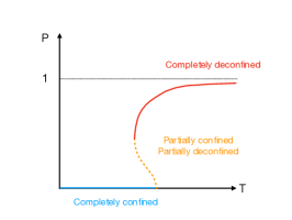
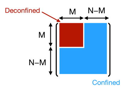
Between confined and deconfined phases of SU(N𝑁N) gauge theory there exists the partially-deconfined phase (equivalently, partially-confined phase), in which a SU(M𝑀M) subgroup deconfines; see Fig. 1. The size of the deconfined sector M𝑀M can change from 0 (complete confinement) to N𝑁N (complete deconfinement) Hanada:2016pwv ; Berenstein:2018lrm ; Hanada:2018zxn ; Hanada:2019czd . The underlying mechanism identified in Ref. Hanada:2020uvt does not depend on the details of the theories. Let us consider large-N𝑁N QCD with Nfsubscript𝑁𝑓N_{f} flavors in the fundamental representation. We take NfNsubscript𝑁𝑓𝑁\frac{N_{f}}{N} sufficiently large and quark masses sufficiently small such that the confinement/deconfinement transition is not of first order, thus resembling the real-world SU(3) QCD Aoki:2006we . In such a case, the partially-deconfined phase is thermodynamically stable; see Ref. Hanada:2019kue for an explicit analysis at finite volume and weak coupling. This opens up the interesting possibility that the so-called QCD crossover region is the partially-deconfined phase.
Refer to caption
Figure 1: In the partially-deconfined phase (equivalently, partially-confined phase), color degrees of freedom split into the confined and deconfined sectors. In this paper, we use M𝑀M to denote the size of the deconfined sector.

In the past, partial deconfinement was studied based on the N𝑁N-dependence of the free energy and entropy. We expect that another characterization of confinement — that we cannot separate quarks without forming a color singlet — is valid for the confined sector in the partially-deconfined phase as well, but there has so far been no direct confirmation. In this paper, we make solid progress regarding this point.

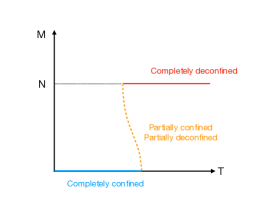
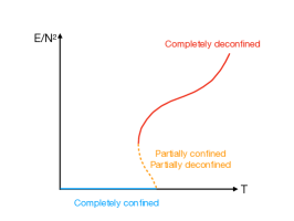
As a concrete example, we consider pure Yang-Mills theory, which exhibits a first-order confinement/deconfinement transition. There is a partially-deconfined saddle separating two minima of the free energy (completely-confined phase and completely-deconfined phase); see Fig. 2. Although this saddle is thermodynamically unstable, it is connected to the stable saddle in QCD as NfNsubscript𝑁𝑓𝑁\frac{N_{f}}{N} or quark mass are varied111 Pure Yang-Mills can be regarded as the heavy-quark-mass limit or NfN0subscript𝑁𝑓𝑁0\frac{N_{f}}{N}\to 0 limit. and we expect qualitative similarity between stable and unstable saddles. In the string-condensation picture, only the SU(M𝑀M) chromo-electric strings are condensed. If we take a probe quark and antiquark from the deconfined sector, then they can interact with condensed strings and should not have the confinement potential. On the other hand, if we take probes from the confined sector, we expect the linear confinement potential, because there are no condensed strings in this sector.
Refer to caption
Refer to caption
Refer to caption
Figure 2: Sketches of the temperature dependence of M𝑀M, EN2𝐸superscript𝑁2\frac{E}{N^{2}} and P𝑃P for the pure Yang-Mills theory. Blue, orange and red lines are completely-confined phase, partially-deconfined saddle (equivalently, partially-confined saddle) and completely-deconfined phase. The partially-deconfined saddle is the maximum of free energy at fixed temperature. See Ref. Hanada:2018zxn for other examples including a thermodynamically stable partially-deconfined phase.

We will test this statement by using a gauge fixing that separates confined and deconfined sectors in a controlled manner. Specifically, we will consider the strong-coupling lattice gauge theory at finite temperature and study the two-point function of the Polyakov loop. There are several reasons we consider this theory. First of all, partial deconfinement is a generic property of gauge theories with confinement/deconfinement transition including this model. Secondly, we can use the Eguchi-Kawai equivalence (large-N𝑁N volume reduction) which makes our numerical simulation tractable. Furthermore, for this particular setup, we can make a few analytic predictions assuming the formation of the flux tube in the confined sector, and we can confirm the prediction numerically. Because such analytic predictions are not available in the continuum limit, we can perform a stronger test by focusing on the strong-coupling lattice gauge theory. The Polyakov loop Tr𝒫(x)Tr𝒫𝑥{\rm Tr}{\cal P}(\vec{x}) is the trace of the holonomy 𝒫(x)𝒫𝑥{\cal P}(\vec{x}) along the temporal circle defined by

𝒫(x)=[Pexp(i𝑑tAt(t,x))]𝒫𝑥delimited-[]P𝑖contour-integraldifferential-d𝑡subscript𝐴𝑡𝑡𝑥\displaystyle{\cal P}(\vec{x})=\left[{\rm P}\exp\left(i\oint dtA_{t}(t,\vec{x})\right)\right] (1)

where PP{\rm P} stands for the path ordering and x𝑥{\vec{x}} is the spatial point. The two-point function decays exponentially in the completely-confined phase as

Tr𝒫(x)Tr𝒫(y)eβσ|xy|,similar-todelimited-⟨⟩Tr𝒫𝑥Tr𝒫𝑦superscript𝑒𝛽𝜎𝑥𝑦\displaystyle\left\langle{\rm Tr}{\cal P}(\vec{x})\cdot{\rm Tr}{\cal P}(\vec{y})\right\rangle\sim e^{-\beta\sigma|\vec{x}-\vec{y}|}, (2)

where β=T1𝛽superscript𝑇1\beta=T^{-1} is the inverse temperature and σ𝜎\sigma is the string tension. We will perform a gauge fixing such that colors split into the confined and deconfined sectors, respectively, and define the Polyakov loops in those sectors, Tr𝒫con(x)Trsubscript𝒫con𝑥{\rm Tr}{\cal P}_{{\rm con}}(\vec{x}) and Tr𝒫dec(x)Trsubscript𝒫dec𝑥{\rm Tr}{\cal P}_{{\rm dec}}(\vec{x}). Then, we show that Tr𝒫con(x)Trsubscript𝒫con𝑥{\rm Tr}{\cal P}_{{\rm con}}(\vec{x}) exhibits the exponential decay

Tr𝒫con(x)Tr𝒫con(y)eβσ|xy|similar-todelimited-⟨⟩Trsubscript𝒫con𝑥Trsubscript𝒫con𝑦superscript𝑒𝛽𝜎𝑥𝑦\displaystyle\left\langle{\rm Tr}{\cal P}_{{\rm con}}(\vec{x})\cdot{\rm Tr}{\cal P}_{{\rm con}}(\vec{y})\right\rangle\sim e^{-\beta\sigma|\vec{x}-\vec{y}|} (3)

with the same string tension σ𝜎\sigma. We also show that

Tr𝒫con(x)Tr𝒫dec(y)eβσ|xy|.similar-todelimited-⟨⟩Trsubscript𝒫con𝑥Trsubscript𝒫dec𝑦superscript𝑒𝛽𝜎𝑥𝑦\displaystyle\left\langle{\rm Tr}{\cal P}_{{\rm con}}(\vec{x})\cdot{\rm Tr}{\cal P}_{{\rm dec}}(\vec{y})\right\rangle\sim e^{-\beta\sigma|\vec{x}-\vec{y}|}. (4)

We interpret the relations (3) and (4) as consequences of the formation of flux tubes and linear confinement in the confined sector. For the strong-coupling lattice gauge theory, we confirm these relations quantitatively, including the concrete value of the string tension σ𝜎\sigma and the overall constant factor.

This paper is organized as follows. In Sec. 2, we use the operator formalism to explain partial deconfinement. In Sec. 3, we define the lattice action and set the simulation strategy. In Sec. 4, we determine the size of the deconfined sector M𝑀M at each simulation point by using the relation between M𝑀M and the phase distribution of the Polyakov loop Hanada:2020uvt . In Sec. 5, we provide evidence of the linear confinement potential in the confined sector of the partially-deconfined phase. Theoretical considerations are provided in Sec. 5.1. Then, numerical evidence is given in Sec. 5.2. We define the Wilson loop equivalent to the two-point function of the Polyakov loop, and study it by using the Eguchi-Kawai equivalence in the large-N𝑁N limit.

2 Theoretical background

Hamiltonian formulation

The meaning of partial deconfinement is clearer if we look directly at quantum states by working in the operator formalism. In this section, we describe the partially-deconfined phase by using the Hamiltonian formulation by Kogut and Susskind Kogut:1974ag . We consider the (3+1)-d Yang-Mills theory with U(N𝑁N) gauge group. The adaptation of this theory to the path-integral formalism, as actually used in our simulations, is described in Sec. 3. The purpose of this section is to explain aspects of partial deconfinement using the string condensation picture Polyakov:1978vu ; Susskind:1979up .

The Kogut-Susskind Hamiltonian consists of the electric and magnetic terms,

H^=H^E+H^B.^𝐻subscript^𝐻Esubscript^𝐻B\displaystyle\hat{H}=\hat{H}_{\rm E}+\hat{H}_{\rm B}. (5)

The electric part of the Hamiltonian becomes

H^E=12nμ=13α=1N2(E^μ,nα)2.subscript^𝐻E12subscript𝑛superscriptsubscript𝜇13superscriptsubscript𝛼1superscript𝑁2superscriptsuperscriptsubscript^𝐸𝜇𝑛𝛼2\displaystyle\hat{H}_{\rm E}=\frac{1}{2}\sum_{\vec{n}}\sum_{\mu=1}^{3}\sum_{\alpha=1}^{N^{2}}\left(\hat{E}_{\mu,\vec{n}}^{\alpha}\right)^{2}. (6)

The magnetic term (plaquette) is dropped in the strong coupling limit Susskind:1979up . The commutation relations are

[U^,U^]=[U^,U^]=[U^,U^]=0.^𝑈^𝑈^𝑈superscript^𝑈superscript^𝑈superscript^𝑈0\displaystyle\left[\hat{U},\hat{U}\right]=\left[\hat{U},\hat{U}^{\dagger}\right]=\left[\hat{U}^{\dagger},\hat{U}^{\dagger}\right]=0. (7)
[E^μ,nα,U^ν,n]=δμνδnnταU^ν,n,[E^μ,nα,U^ν,n]=δμνδnnU^ν,nτα,formulae-sequencesuperscriptsubscript^𝐸𝜇𝑛𝛼subscript^𝑈𝜈superscript𝑛subscript𝛿𝜇𝜈subscript𝛿𝑛superscript𝑛subscript𝜏𝛼subscript^𝑈𝜈superscript𝑛superscriptsubscript^𝐸𝜇𝑛𝛼subscriptsuperscript^𝑈𝜈superscript𝑛subscript𝛿𝜇𝜈subscript𝛿𝑛superscript𝑛superscriptsubscript^𝑈𝜈superscript𝑛subscript𝜏𝛼\displaystyle\left[\hat{E}_{\mu,\vec{n}}^{\alpha},\hat{U}_{\nu,\vec{n}^{\prime}}\right]=\delta_{\mu\nu}\delta_{\vec{n}\vec{n}^{\prime}}\tau_{\alpha}\hat{U}_{\nu,\vec{n}^{\prime}},\qquad\left[\hat{E}_{\mu,\vec{n}}^{\alpha},\hat{U}^{\dagger}_{\nu,\vec{n}^{\prime}}\right]=-\delta_{\mu\nu}\delta_{\vec{n}\vec{n}^{\prime}}\hat{U}_{\nu,\vec{n}^{\prime}}^{\dagger}\tau_{\alpha}, (8)
[E^μ,nα,E^ν,nβ]=ifαβγδμνδnnE^ν,nγ,superscriptsubscript^𝐸𝜇𝑛𝛼superscriptsubscript^𝐸𝜈superscript𝑛𝛽𝑖superscript𝑓𝛼𝛽𝛾subscript𝛿𝜇𝜈subscript𝛿𝑛superscript𝑛subscriptsuperscript^𝐸𝛾𝜈superscript𝑛\displaystyle\left[\hat{E}_{\mu,\vec{n}}^{\alpha},\hat{E}_{\nu,\vec{n}^{\prime}}^{\beta}\right]=-if^{\alpha\beta\gamma}\delta_{\mu\nu}\delta_{\vec{n}\vec{n}^{\prime}}\hat{E}^{\gamma}_{\nu,\vec{n}^{\prime}}, (9)

where fαβγsuperscript𝑓𝛼𝛽𝛾f^{\alpha\beta\gamma} is the structure constant of U(N𝑁N), and

α=1N2τpqατrsα=δpsδqrN,α=1N2(τατα)pq=δpq.formulae-sequencesuperscriptsubscript𝛼1superscript𝑁2subscriptsuperscript𝜏𝛼𝑝𝑞subscriptsuperscript𝜏𝛼𝑟𝑠subscript𝛿𝑝𝑠subscript𝛿𝑞𝑟𝑁superscriptsubscript𝛼1superscript𝑁2subscriptsuperscript𝜏𝛼superscript𝜏𝛼𝑝𝑞subscript𝛿𝑝𝑞\displaystyle\sum_{\alpha=1}^{N^{2}}\tau^{\alpha}_{pq}\tau^{\alpha}_{rs}=\frac{\delta_{ps}\delta_{qr}}{N},\qquad\sum_{\alpha=1}^{N^{2}}\left(\tau^{\alpha}\tau^{\alpha}\right)_{pq}=\delta_{pq}. (10)

The ground state of this string-coupling lattice gauge theory Hamiltonian |g.s.|{\rm g.s.}\rangle satisfies E^μ,nα|g.s.=0\hat{E}_{\mu,\vec{n}}^{\alpha}|{\rm g.s.}\rangle=0 for any α,μ𝛼𝜇\alpha,\mu and n𝑛\vec{n}. Hence, let us use the notation |E=0ket𝐸0|E=0\rangle to denote the ground state.

The operator U^μ,nsubscript^𝑈𝜇𝑛\hat{U}_{\mu,\vec{n}} is interpreted as the coordinate of the group manifold U(N𝑁N) for the link variable on the site n𝑛\vec{n} in the μ𝜇\mu-direction. The operators U^^𝑈\hat{U} and E^^𝐸\hat{E} are defined on the extended Hilbert space extsubscriptext\mathcal{H}_{\rm ext} that contains gauge non-singlet modes. A convenient basis of extsubscriptext\mathcal{H}_{\rm ext} is the coordinate representation,

ext=μ,nμ,nμ,n(gU(N)|gμ,n),\displaystyle{\cal H}_{\rm ext}=\otimes_{\mu,\vec{n}}{\cal H}_{\mu,\vec{n}}\sim\otimes_{\mu,\vec{n}}\left(\oplus_{g\in{\rm U}(N)}|g\rangle_{\mu,\vec{n}}\right), (11)

where

U^μ,n|gμ,n=g|gμ,ngU(N).formulae-sequencesubscript^𝑈𝜇𝑛subscriptket𝑔𝜇𝑛𝑔subscriptket𝑔𝜇𝑛𝑔U𝑁\displaystyle\hat{U}_{\mu,\vec{n}}|g\rangle_{\mu,\vec{n}}=g|g\rangle_{\mu,\vec{n}}\qquad g\in{\rm U}(N). (12)

More precisely, we will consider only the Hilbert space of square-integrable wave functions on U(N𝑁N): μ,n=L2(U(N))subscript𝜇𝑛superscript𝐿2U𝑁{\cal H}_{\mu,\vec{n}}=L^{2}({\rm U}(N)), where L2(U(N))superscript𝐿2U𝑁L^{2}({\rm U}(N)) is the set of square-integrable functions from U(N)U𝑁{\rm U}(N) to {\mathbb{C}}. The ground state is the constant mode,

|E=0=μ,n|E=0μ,n,|E=0μ,n=1volU(N)U(N)dg|gμ,n.\displaystyle|E=0\rangle=\otimes_{\mu,\vec{n}}|E=0\rangle_{\mu,\vec{n}},\qquad|E=0\rangle_{\mu,\vec{n}}=\frac{1}{\sqrt{{\rm volU}(N)}}\int_{{\rm U}(N)}dg|g\rangle_{\mu,\vec{n}}. (13)

Namely, the wave function g|E=0inner-product𝑔𝐸0\langle g|E=0\rangle is constant.

Let G=n[U(N)]n𝐺subscriptproduct𝑛subscriptdelimited-[]U𝑁𝑛G=\prod_{\vec{n}}[{\rm U}(N)]_{\vec{n}} be the group of all local gauge transformations. Gauge transformation by Ω^=nΩ^n\hat{\Omega}=\otimes_{\vec{n}}\hat{\Omega}_{\vec{n}} is defined by

Ω^(μ,n|gμ,n)=μ,n(Ω^n|gμ,n)=μ,n|ΩngΩn1μ,n.\displaystyle\hat{\Omega}\left(\otimes_{\mu,\vec{n}}|g\rangle_{\mu,\vec{n}}\right)=\otimes_{\mu,\vec{n}}\left(\hat{\Omega}_{\vec{n}}|g\rangle_{\mu,\vec{n}}\right)=\otimes_{\mu,\vec{n}}|\Omega_{\vec{n}}g\Omega_{\vec{n}}^{-1}\rangle_{\mu,\vec{n}}. (14)

Note that the ground state is gauge-invariant:

Ω^|E=0=|E=0.^Ωket𝐸0ket𝐸0\displaystyle\hat{\Omega}|E=0\rangle=|E=0\rangle. (15)

We can define the projection operator to the gauge-invariant Hilbert space invsubscriptinv\mathcal{H}_{\rm inv} as

π^=1VolGG𝑑ΩΩ^,^𝜋1Vol𝐺subscript𝐺differential-dΩ^Ω\displaystyle\hat{\pi}=\frac{1}{{\rm Vol}G}\int_{G}d\Omega\hat{\Omega}, (16)

where the integral is taken by using the Haar measure. By using this projection operator, canonical partition function at temperature T𝑇T can be written in two ways as

Z(T)=Trinv(eH^/T)=Trext(π^eH^/T).𝑍𝑇subscriptTrsubscriptinvsuperscript𝑒^𝐻𝑇subscriptTrsubscriptext^𝜋superscript𝑒^𝐻𝑇\displaystyle Z(T)={\rm Tr}_{\mathcal{H}_{\rm inv}}\left(e^{-\hat{H}/T}\right)={\rm Tr}_{\mathcal{H}_{\rm ext}}\left(\hat{\pi}e^{-\hat{H}/T}\right). (17)

The latter expression is directly related to the path-integral formalism with gauge field Atsubscript𝐴𝑡A_{t}, as shown in Appendix C. The U(N𝑁N)-element ΩΩ\Omega corresponds to the Polyakov loop in the path-integral formalism Hanada:2020uvt . The insertion of π^^𝜋\hat{\pi} means we should identify the states connected by gauge transformation, as we identify field configurations connected by gauge transformation in the classical theory. In other words, all states on the gauge orbit are physically equivalent. This makes the meaning of ‘gauge fixing’ in the extended Hilbert space clear: it selects a point from the gauge orbit, just as in the path-integral formalism or even in the classical theory. In the SU(M𝑀M)-deconfined phase, we can take a gauge such that the upper-left M×M𝑀𝑀M\times M block is deconfined, as in Fig. 1.

Strings and Interactions

A closed string is created by the Wilson loop W^C(closed)=Tr(U^μ,n^U^ν,n^+μ^)subscriptsuperscript^𝑊closed𝐶Trsubscript^𝑈𝜇^𝑛subscript^𝑈𝜈^𝑛^𝜇\hat{W}^{\rm(closed)}_{C}={\rm Tr}(\hat{U}_{\mu,\hat{n}}\hat{U}_{\nu,\hat{n}+\hat{\mu}}\cdots), where the product of U^^𝑈\hat{U}’s in the trace is taken along the closed path C𝐶C. An open string is created by the open Wilson line along an open path Csuperscript𝐶C^{\prime}, denoted by W^C(open)subscriptsuperscript^𝑊opensuperscript𝐶\hat{W}^{\rm(open)}_{C^{\prime}}, which is a product of U^^𝑈\hat{U}’s without trace. The closed string is gauge invariant.

Suppose that there is a closed loop without self-intersection (i.e. no link appears twice). Then, the state |WC(closed)W^C(closed)|0ketsubscriptsuperscript𝑊closed𝐶subscriptsuperscript^𝑊closed𝐶ket0|W^{\rm(closed)}_{C}\rangle\equiv\hat{W}^{\rm(closed)}_{C}|0\rangle is an energy eigenstate, and the energy is L2𝐿2\frac{L}{2}, where L𝐿L is the length of the loop (i.e., the number of links consisting the loop). This can be seen as follows. Firstly, note that

α(E^μ,nα)2W^C(closed)|E=0=α[E^μ,nα,[E^μ,nα,W^C(closed)]]|E=0.subscript𝛼superscriptsuperscriptsubscript^𝐸𝜇𝑛𝛼2superscriptsubscript^𝑊𝐶closedket𝐸0subscript𝛼superscriptsubscript^𝐸𝜇𝑛𝛼superscriptsubscript^𝐸𝜇𝑛𝛼superscriptsubscript^𝑊𝐶closedket𝐸0\displaystyle\sum_{\alpha}\left(\hat{E}_{\mu,\vec{n}}^{\alpha}\right)^{2}\hat{W}_{C}^{\rm(closed)}|E=0\rangle=\sum_{\alpha}\left[\hat{E}_{\mu,\vec{n}}^{\alpha},\left[\hat{E}_{\mu,\vec{n}}^{\alpha},\hat{W}_{C}^{\rm(closed)}\right]\right]|E=0\rangle. (18)

E^μ,nαsuperscriptsubscript^𝐸𝜇𝑛𝛼\hat{E}_{\mu,\vec{n}}^{\alpha} commutes with W^C(closed)subscriptsuperscript^𝑊closed𝐶\hat{W}^{\rm(closed)}_{C} unless the latter contains U^μ,nsubscript^𝑈𝜇𝑛\hat{U}_{\mu,\vec{n}} or U^μ,nsubscriptsuperscript^𝑈𝜇𝑛\hat{U}^{\dagger}_{\mu,\vec{n}}. When U^μ,nsubscript^𝑈𝜇𝑛\hat{U}_{\mu,\vec{n}} is contained,

α[E^μ,nα,[E^μ,nα,W^C(closed)]]|E=0subscript𝛼superscriptsubscript^𝐸𝜇𝑛𝛼superscriptsubscript^𝐸𝜇𝑛𝛼superscriptsubscript^𝑊𝐶closedket𝐸0\displaystyle\sum_{\alpha}\left[\hat{E}_{\mu,\vec{n}}^{\alpha},\left[\hat{E}_{\mu,\vec{n}}^{\alpha},\hat{W}_{C}^{\rm(closed)}\right]\right]|E=0\rangle =αTr([E^μ,nα,[E^μ,nα,U^μ,n^]]U^ν,n^+μ^)|E=0absentsubscript𝛼Trsuperscriptsubscript^𝐸𝜇𝑛𝛼superscriptsubscript^𝐸𝜇𝑛𝛼subscript^𝑈𝜇^𝑛subscript^𝑈𝜈^𝑛^𝜇ket𝐸0\displaystyle=\sum_{\alpha}{\rm Tr}\left(\left[\hat{E}_{\mu,\vec{n}}^{\alpha},\left[\hat{E}_{\mu,\vec{n}}^{\alpha},\hat{U}_{\mu,\hat{n}}\right]\right]\hat{U}_{\nu,\hat{n}+\hat{\mu}}\cdots\right)|E=0\rangle
=αTr(ταταU^μ,n^U^ν,n^+μ^)|E=0absentsubscript𝛼Trsuperscript𝜏𝛼superscript𝜏𝛼subscript^𝑈𝜇^𝑛subscript^𝑈𝜈^𝑛^𝜇ket𝐸0\displaystyle=\sum_{\alpha}{\rm Tr}\left(\tau^{\alpha}\tau^{\alpha}\hat{U}_{\mu,\hat{n}}\hat{U}_{\nu,\hat{n}+\hat{\mu}}\cdots\right)|E=0\rangle
=Tr(U^μ,n^U^ν,n^+μ^)|E=0absentTrsubscript^𝑈𝜇^𝑛subscript^𝑈𝜈^𝑛^𝜇ket𝐸0\displaystyle={\rm Tr}\left(\hat{U}_{\mu,\hat{n}}\hat{U}_{\nu,\hat{n}+\hat{\mu}}\cdots\right)|E=0\rangle
=W^C(closed)|E=0.absentsuperscriptsubscript^𝑊𝐶closedket𝐸0\displaystyle=\hat{W}_{C}^{\rm(closed)}|E=0\rangle. (19)

The same holds when U^μ,n^subscriptsuperscript^𝑈𝜇^𝑛\hat{U}^{\dagger}_{\mu,\hat{n}} is contained. Therefore, H^E|WC(closed)=L2|WC(closed)subscript^𝐻Eketsubscriptsuperscript𝑊closed𝐶𝐿2ketsubscriptsuperscript𝑊closed𝐶\hat{H}_{\rm E}|W^{\rm(closed)}_{C}\rangle=\frac{L}{2}|W^{\rm(closed)}_{C}\rangle. The same holds for any multi-string states, including closed or open strings, as long as there is no intersection.

Next, suppose a link U^μ,nsubscript^𝑈𝜇𝑛\hat{U}_{\mu,\vec{n}} appears twice in the loop, while other links appear only once. Let us write such a loop as Tr(V^1U^μ,nV^2U^μ,n)Trsubscript^𝑉1subscript^𝑈𝜇𝑛subscript^𝑉2subscript^𝑈𝜇𝑛{\rm Tr}(\hat{V}_{1}\hat{U}_{\mu,\vec{n}}\hat{V}_{2}\hat{U}_{\mu,\vec{n}}). Then,

α[E^μ,nα,[E^μ,nα,Tr(V^1U^μ,nV^2U^μ,n)]]|E=0subscript𝛼superscriptsubscript^𝐸𝜇𝑛𝛼superscriptsubscript^𝐸𝜇𝑛𝛼Trsubscript^𝑉1subscript^𝑈𝜇𝑛subscript^𝑉2subscript^𝑈𝜇𝑛ket𝐸0\displaystyle\sum_{\alpha}\left[\hat{E}_{\mu,\vec{n}}^{\alpha},\left[\hat{E}_{\mu,\vec{n}}^{\alpha},{\rm Tr}(\hat{V}_{1}\hat{U}_{\mu,\vec{n}}\hat{V}_{2}\hat{U}_{\mu,\vec{n}})\right]\right]|E=0\rangle
=2Tr(V^1U^μ,nV^2U^μ,n)|E=0+2αTr(V^1[E^μ,nα,U^μ,n]V^2[E^μ,nα,U^μ,n])|E=0absent2Trsubscript^𝑉1subscript^𝑈𝜇𝑛subscript^𝑉2subscript^𝑈𝜇𝑛ket𝐸02subscript𝛼Trsubscript^𝑉1superscriptsubscript^𝐸𝜇𝑛𝛼subscript^𝑈𝜇𝑛subscript^𝑉2superscriptsubscript^𝐸𝜇𝑛𝛼subscript^𝑈𝜇𝑛ket𝐸0\displaystyle=2{\rm Tr}(\hat{V}_{1}\hat{U}_{\mu,\vec{n}}\hat{V}_{2}\hat{U}_{\mu,\vec{n}})|E=0\rangle+2\sum_{\alpha}{\rm Tr}(\hat{V}_{1}[\hat{E}_{\mu,\vec{n}}^{\alpha},\hat{U}_{\mu,\vec{n}}]\hat{V}_{2}[\hat{E}_{\mu,\vec{n}}^{\alpha},\hat{U}_{\mu,\vec{n}}])|E=0\rangle
=2Tr(V^1U^μ,nV^2U^μ,n)|E=0+2αTr(V^1ταU^μ,nV^2ταU^μ,n)|E=0absent2Trsubscript^𝑉1subscript^𝑈𝜇𝑛subscript^𝑉2subscript^𝑈𝜇𝑛ket𝐸02subscript𝛼Trsubscript^𝑉1superscript𝜏𝛼subscript^𝑈𝜇𝑛subscript^𝑉2superscript𝜏𝛼subscript^𝑈𝜇𝑛ket𝐸0\displaystyle=2{\rm Tr}(\hat{V}_{1}\hat{U}_{\mu,\vec{n}}\hat{V}_{2}\hat{U}_{\mu,\vec{n}})|E=0\rangle+2\sum_{\alpha}{\rm Tr}(\hat{V}_{1}\tau^{\alpha}\hat{U}_{\mu,\vec{n}}\hat{V}_{2}\tau^{\alpha}\hat{U}_{\mu,\vec{n}})|E=0\rangle
=2Tr(V^1U^μ,nV^2U^μ,n)|E=0+2NTr(V^1U^μ,n)Tr(V^2U^μ,n)|E=0.absent2Trsubscript^𝑉1subscript^𝑈𝜇𝑛subscript^𝑉2subscript^𝑈𝜇𝑛ket𝐸02𝑁Trsubscript^𝑉1subscript^𝑈𝜇𝑛Trsubscript^𝑉2subscript^𝑈𝜇𝑛ket𝐸0\displaystyle=2{\rm Tr}(\hat{V}_{1}\hat{U}_{\mu,\vec{n}}\hat{V}_{2}\hat{U}_{\mu,\vec{n}})|E=0\rangle+\frac{2}{N}{\rm Tr}(\hat{V}_{1}\hat{U}_{\mu,\vec{n}}){\rm Tr}(\hat{V}_{2}\hat{U}_{\mu,\vec{n}})|E=0\rangle. (20)

Therefore,

H^E(Tr(V^1U^μ,nV^2U^μ,n)|E=0)subscript^𝐻𝐸Trsubscript^𝑉1subscript^𝑈𝜇𝑛subscript^𝑉2subscript^𝑈𝜇𝑛ket𝐸0\displaystyle\hat{H}_{E}\left({\rm Tr}(\hat{V}_{1}\hat{U}_{\mu,\vec{n}}\hat{V}_{2}\hat{U}_{\mu,\vec{n}})|E=0\rangle\right)
=L2Tr(V^1U^μ,nV^2U^μ,n)|E=0+1NTr(V^1U^μ,n)Tr(V^2U^μ,n)|E=0.absent𝐿2Trsubscript^𝑉1subscript^𝑈𝜇𝑛subscript^𝑉2subscript^𝑈𝜇𝑛ket𝐸01𝑁Trsubscript^𝑉1subscript^𝑈𝜇𝑛Trsubscript^𝑉2subscript^𝑈𝜇𝑛ket𝐸0\displaystyle=\frac{L}{2}{\rm Tr}(\hat{V}_{1}\hat{U}_{\mu,\vec{n}}\hat{V}_{2}\hat{U}_{\mu,\vec{n}})|E=0\rangle+\frac{1}{N}{\rm Tr}(\hat{V}_{1}\hat{U}_{\mu,\vec{n}}){\rm Tr}(\hat{V}_{2}\hat{U}_{\mu,\vec{n}})|E=0\rangle. (21)

The second term can be understood as the splitting of a string into two strings. In the same manner, we can show that two strings can be joined to form one string at an intersection,

H^E(Tr(V^1U^μ,n)Tr(V^2U^μ,n)|E=0)subscript^𝐻𝐸Trsubscript^𝑉1subscript^𝑈𝜇𝑛Trsubscript^𝑉2subscript^𝑈𝜇𝑛ket𝐸0\displaystyle\hat{H}_{E}\left({\rm Tr}(\hat{V}_{1}\hat{U}_{\mu,\vec{n}}){\rm Tr}(\hat{V}_{2}\hat{U}_{\mu,\vec{n}})|E=0\rangle\right)
=L2Tr(V^1U^μ,n)Tr(V^2U^μ,n)|E=0+1NTr(V^1U^μ,nV^2U^μ,n)|E=0.absent𝐿2Trsubscript^𝑉1subscript^𝑈𝜇𝑛Trsubscript^𝑉2subscript^𝑈𝜇𝑛ket𝐸01𝑁Trsubscript^𝑉1subscript^𝑈𝜇𝑛subscript^𝑉2subscript^𝑈𝜇𝑛ket𝐸0\displaystyle=\frac{L}{2}{\rm Tr}(\hat{V}_{1}\hat{U}_{\mu,\vec{n}}){\rm Tr}(\hat{V}_{2}\hat{U}_{\mu,\vec{n}})|E=0\rangle+\frac{1}{N}{\rm Tr}(\hat{V}_{1}\hat{U}_{\mu,\vec{n}}\hat{V}_{2}\hat{U}_{\mu,\vec{n}})|E=0\rangle. (22)

In general, such splitting and joining can take place at any intersection.

Confinement

Let us consider low-energy gauge-invariant states consisting of a small number of closed strings with total length LN0similar-to𝐿superscript𝑁0L\sim N^{0}. Then, there is at most order N0superscript𝑁0N^{0} number of intersections. The interaction (splitting or joining) at each intersection is suppressed by 1N1𝑁\frac{1}{N}, and hence the interaction is negligible at large N𝑁N. The energy of the system is simply L2𝐿2\frac{L}{2}. Such states are in the confined phase.

If we introduce a probe quark-antiquark pair connected by the open Wilson line, the energy increases linearly as Eqq¯=L2subscript𝐸𝑞¯𝑞𝐿2E_{q\bar{q}}=\frac{L}{2}. This leads to the linear confinement potential.

Deconfinement and string condensation

In the deconfined phase Polyakov:1978vu ; Susskind:1979up , long strings with length of order N2superscript𝑁2N^{2} condense. There are many intersections, and thus the 1/N1𝑁1/N-suppressed interactions accompanying each intersection pile up and become non-negligible as a whole. Intuitively, if we introduce a short open string, it interacts with a condensed long string and forms a long open string, which allows us to separate quark and antiquark without making the string longer.

Partial deconfinement

Let U^decsubscript^𝑈dec\hat{U}_{\rm dec} be the SU(M𝑀M)-subsector. The SU(M𝑀M)-deconfined states can be constructed by acting with long traces of U^decsubscript^𝑈dec\hat{U}_{\rm dec}’s on |E=0ket𝐸0|E=0\rangle Hanada:2019czd .222See Refs.  Hanada:2021ipb ; Hanada:2021swb ; Gautam:2022akq for more general characterization. By using the Wilson loops restricted to the SU(M𝑀M)-subsector

W^dec,C=Tr(U^dec;μ,nU^dec;ν,n+μ^),subscript^𝑊dec𝐶Trsubscript^𝑈dec𝜇𝑛subscript^𝑈dec𝜈𝑛^𝜇\displaystyle\hat{W}_{{\rm dec},C}={\rm Tr}(\hat{U}_{{\rm dec};\mu,\vec{n}}\hat{U}_{{\rm dec};\nu,\vec{n}+\hat{\mu}}\cdots), (23)

we can construct multi-string states

W^dec,CW^dec,C|E=0,subscript^𝑊dec𝐶subscript^𝑊decsuperscript𝐶ket𝐸0\displaystyle\hat{W}_{{\rm dec},C}\hat{W}_{{\rm dec},C^{\prime}}\cdots|E=0\rangle, (24)

and then we can take a linear combination of such states. Such states are SU(M𝑀M)-invariant, but not SU(N𝑁N)-invariant. If we want to get an SU(N𝑁N)-invariant state, we can act with the projector π^^𝜋\hat{\pi}.

The reason that such a phase is favored is understood from (17Hanada:2020uvt . We write the projection operator π^^𝜋\hat{\pi} explicitly as

Z(T)=1Vol(G)G𝑑ΩTrext(Ω^eH^/T).𝑍𝑇1Vol𝐺subscript𝐺differential-dΩsubscriptTrsubscriptext^Ωsuperscript𝑒^𝐻𝑇\displaystyle Z(T)=\frac{1}{{\rm Vol}(G)}\int_{G}d\Omega{\rm Tr}_{\mathcal{H}_{\rm ext}}\left(\hat{\Omega}e^{-\hat{H}/T}\right). (25)

From this expression, we can see that each energy eigenstate333 Here, E𝐸E is the energy and not the electric field. For the ground state, we used the notation |E=0ket𝐸0|E=0\rangle by meaning that the electric field E𝐸E is zero. Coincidentally, the energy of the ground state is also zero. |Eextket𝐸subscriptext|E\rangle\in\mathcal{H}_{\rm ext} has a contribution

1Vol(G)G𝑑ΩeE/TE|Ω^|E.1Vol𝐺subscript𝐺differential-dΩsuperscript𝑒𝐸𝑇quantum-operator-product𝐸^Ω𝐸\displaystyle\frac{1}{{\rm Vol}(G)}\int_{G}d\Omega e^{-E/T}\langle E|\hat{\Omega}|E\rangle. (26)

If |Eket𝐸|E\rangle is an SU(M𝑀M)-deconfined state, we have Ω^|E=|E^Ωket𝐸ket𝐸\hat{\Omega}|E\rangle=|E\rangle for ΩU(NM)ΩU𝑁𝑀\Omega\in{\rm U}(N-M), such that ΩΩ\Omega does not act on the SU(M𝑀M)-subsector. Hence, there is an enhancement factor Vol(U(NM))e(NM)2similar-toVolU𝑁𝑀superscript𝑒superscript𝑁𝑀2{\rm Vol}({\rm U}(N-M))\sim e^{(N-M)^{2}}. This factor makes smaller M𝑀M more favorable. At each fixed energy, this factor and other entropy factors compete and a certain value of M𝑀M between 00 and N𝑁N is determined as the most favorable value that maximizes the entropy. This is essentially the same mechanism as the Bose-Einstein condensation Hanada:2020uvt .

Let U^consubscript^𝑈con\hat{U}_{\rm con} be the other N2M2superscript𝑁2superscript𝑀2N^{2}-M^{2} elements. Operators that consist of a number LO(N0)similar-to𝐿𝑂superscript𝑁0L\sim O(N^{0}) of U^consubscript^𝑈con\hat{U}_{\rm con}’s increase the energy by L2𝐿2\frac{L}{2}. They cannot be joined to the condensed strings. The energy eigenstate remains an energy eigenstate. Naturally, we expect that the color flux in the confined sector forms a flux tube and exhibits the linear potential Eqq¯=L2subscript𝐸𝑞¯𝑞𝐿2E_{q\bar{q}}=\frac{L}{2} while the deconfined sector does not. We will discuss this later, together with numerical results.

3 Methods

We will perform our simulations on a lattice-discretized model of U(N𝑁N) Yang-Mills theory. Our simulations will involve constraining specific quantities so that we can remain in the partially-deconfined phase, and also so that we can separate the confined and deconfined sectors. Specifically, we use the Eguchi-Kawai model, which is equivalent to U(N𝑁N) Yang-Mills theory in the large-N𝑁N limit. The introduction of the constraints amounts to the study of the microcanonical ensemble rather than canonical ensemble, plus gauge fixing. Simulations of lattice gauge theories in the microcanonical ensemble (where the energy is fixed, instead of the temperature) Langfeld:2012ah play a very important role in the numerical study of phase transitions Aarts:2023vsf .

3.1 The lattice regularization

3.1.1 Path-integral formulation

To set up our lattice model, we will begin with the path integral formulation. We consider Yang-Mills theory on a d𝑑d-dimensional spatial lattice with continuous time t𝑡t. We will focus on d=3𝑑3d=3. Let n𝑛\vec{n} be the spatial points labeled by d𝑑d integers, and Uμ,n(t)subscript𝑈𝜇𝑛𝑡U_{\mu,\vec{n}}(t) be the U(N𝑁N) link variable on the link connecting n𝑛\vec{n} and n+μ^𝑛^𝜇\vec{n}+\hat{\mu}. Here, μ^^𝜇\hat{\mu} is the unit vector along the μ𝜇\mu-direction. The gauge transformation is defined by

Uμ,n(t)Λn1(t)Uμ,n(t)Λn+μ^(t).subscript𝑈𝜇𝑛𝑡superscriptsubscriptΛ𝑛1𝑡subscript𝑈𝜇𝑛𝑡subscriptΛ𝑛^𝜇𝑡\displaystyle U_{\mu,\vec{n}}(t)\to\Lambda_{\vec{n}}^{-1}(t)U_{\mu,\vec{n}}(t)\Lambda_{\vec{n}+\hat{\mu}}(t). (27)

Here Λn(t)subscriptΛ𝑛𝑡\Lambda_{\vec{n}}(t) and Λn+μ^(t)subscriptΛ𝑛^𝜇𝑡\Lambda_{\vec{n}+\hat{\mu}}(t) are N×N𝑁𝑁N\times N unitary matrices that describe the local gauge transformation at points n𝑛\vec{n} and n+μ^𝑛^𝜇\vec{n}+\hat{\mu}, respectively. We introduce a gauge field An(t)subscript𝐴𝑛𝑡A_{\vec{n}}(t) that transforms as

An(t)Λn1(t)An(t)Λn(t)+iΛn1(t)tΛn(t).subscript𝐴𝑛𝑡superscriptsubscriptΛ𝑛1𝑡subscript𝐴𝑛𝑡subscriptΛ𝑛𝑡𝑖superscriptsubscriptΛ𝑛1𝑡subscript𝑡subscriptΛ𝑛𝑡\displaystyle A_{\vec{n}}(t)\to\Lambda_{\vec{n}}^{-1}(t)A_{\vec{n}}(t)\Lambda_{\vec{n}}(t)+i\Lambda_{\vec{n}}^{-1}(t)\partial_{t}\Lambda_{\vec{n}}(t). (28)

The covariant derivative DtUμ,nsubscript𝐷𝑡subscript𝑈𝜇𝑛D_{t}U_{\mu,\vec{n}}, which transform as DtUμ,nΛn1(DtUμ,n)Λn+μ^subscript𝐷𝑡subscript𝑈𝜇𝑛superscriptsubscriptΛ𝑛1subscript𝐷𝑡subscript𝑈𝜇𝑛subscriptΛ𝑛^𝜇D_{t}U_{\mu,\vec{n}}\to\Lambda_{\vec{n}}^{-1}(D_{t}U_{\mu,\vec{n}})\Lambda_{\vec{n}+\hat{\mu}}, is defined by

DtUμ,n=tUμ,niAnUμ,n+iUμ,nAn+μ^.subscript𝐷𝑡subscript𝑈𝜇𝑛subscript𝑡subscript𝑈𝜇𝑛𝑖subscript𝐴𝑛subscript𝑈𝜇𝑛𝑖subscript𝑈𝜇𝑛subscript𝐴𝑛^𝜇\displaystyle D_{t}U_{\mu,\vec{n}}=\partial_{t}U_{\mu,\vec{n}}-iA_{\vec{n}}U_{\mu,\vec{n}}+iU_{\mu,\vec{n}}A_{\vec{n}+\hat{\mu}}. (29)

We will work in the strong coupling limit, by which we mean that the action contains only the electric term and not the magnetic term. Hence the Euclidean action at temperature T=β1𝑇superscript𝛽1T=\beta^{-1} is444 We use the same symbol S𝑆S for the action and entropy, assuming the risk of confusion is low.

S=12g2n0β𝑑tTr((DtUμ,n(t))(DtUμ,n(t))).𝑆12superscript𝑔2subscript𝑛superscriptsubscript0𝛽differential-d𝑡Trsubscript𝐷𝑡subscript𝑈𝜇𝑛𝑡superscriptsubscript𝐷𝑡subscript𝑈𝜇𝑛𝑡\displaystyle S=\frac{1}{2g^{2}}\sum_{\vec{n}}\int_{0}^{\beta}dt{\rm Tr}\left((D_{t}U_{\mu,\vec{n}}(t))(D_{t}U_{\mu,\vec{n}}(t))^{\dagger}\right). (30)

The operator Ω^^Ω\hat{\Omega} in (25) corresponds to the Polyakov loop in the path-integral formalism Hanada:2020uvt (see Appendix C). In the large-N𝑁N limit, the distribution of the phases of the Polyakov loop is related to the symmetry of the typical quantum states dominating the partition function. The size of the deconfined sector M𝑀M can be determined from the distribution of the phases Hanada:2020uvt , as explained in Sec. 4.

3.1.2 Eguchi-Kawai reduction

In the large-N𝑁N limit, some features of the strong-coupling lattice gauge theory do not depend on the lattice size. Therefore, we can use the single-site model, which is called the Eguchi-Kawai model, to learn about the infinite-volume theory. We use conventions close to those in Ref. Hanada:2014noa .

In the Eguchi-Kawai model, we have only one spatial point, so we drop n𝑛\vec{n} from the expressions for the strong-coupling lattice gauge theory. We will employ the gauge field A𝐴A and unitary link variables Uμsubscript𝑈𝜇U_{\mu}, both of which are function of (Euclidean) time t𝑡t. The gauge transformation is defined by

UμΛ1UμΛsubscript𝑈𝜇superscriptΛ1subscript𝑈𝜇Λ\displaystyle U_{\mu}\to\Lambda^{-1}U_{\mu}\Lambda (31)

and

AΛ1AΛ+iΛ1tΛ.𝐴superscriptΛ1𝐴Λ𝑖superscriptΛ1subscript𝑡Λ\displaystyle A\to\Lambda^{-1}A\Lambda+i\Lambda^{-1}\partial_{t}\Lambda. (32)

The covariant derivative DtUμsubscript𝐷𝑡subscript𝑈𝜇D_{t}U_{\mu}, which transform as DtUμΛ1(DtUμ)Λsubscript𝐷𝑡subscript𝑈𝜇superscriptΛ1subscript𝐷𝑡subscript𝑈𝜇ΛD_{t}U_{\mu}\to\Lambda^{-1}(D_{t}U_{\mu})\Lambda, is defined by

DtUμ=tUμi[A,Uμ].subscript𝐷𝑡subscript𝑈𝜇subscript𝑡subscript𝑈𝜇𝑖𝐴subscript𝑈𝜇\displaystyle D_{t}U_{\mu}=\partial_{t}U_{\mu}-i[A,U_{\mu}]. (33)

The Euclidean action is

S=12g20β𝑑tTr(DtUμ)2.𝑆12superscript𝑔2superscriptsubscript0𝛽differential-d𝑡Trsuperscriptsubscript𝐷𝑡subscript𝑈𝜇2\displaystyle S=\frac{1}{2g^{2}}\int_{0}^{\beta}dt{\rm Tr}(D_{t}U_{\mu})^{2}. (34)

This action is invariant under the global (i.e. t𝑡t-independent) U(1)d center symmetry generated by

UμeiθμUμ.subscript𝑈𝜇superscript𝑒𝑖subscript𝜃𝜇subscript𝑈𝜇\displaystyle U_{\mu}\to e^{i\theta_{\mu}}U_{\mu}. (35)

As long as this symmetry is unbroken, the Eguchi-Kawai model and infinite-volume lattice are equivalent, in the sense that various properly-normalized quantities agree. This is the so-called Eguchi-Kawai equivalence Eguchi:1982nm .555 In the original work by Eguchi and Kawai, all dimensions including time are reduced to a point. In most references, ‘Eguchi-Kawai model’ and ‘Eguchi-Kawai equivalence’ are used for the original setup.

In the strong coupling limit, the center symmetry is not spontaneously broken. To confirm this in our simulations as a sanity check, we calculated the Wilson loop wrapped on the spatial direction,

1Nntdμ,d|TrUμ,t|.1𝑁subscript𝑛𝑡𝑑subscript𝜇𝑑Trsubscript𝑈𝜇𝑡\displaystyle\frac{1}{Nn_{t}d}\sum_{\mu,d}|{\rm Tr}U_{\mu,t}|. (36)

If the center symmetry is not broken, this quantity should be zero up to 1/N1𝑁1/N-suppressed terms. Our simulations affirmed this.

3.1.3 Gauge fixing

To make the separation to confined and deconfined phases easier, we take the static diagonal gauge (used in Ref. Watanabe:2020ufk for the same purpose),

A=1βdiag(α1,,αN),π<αiπ.formulae-sequence𝐴1𝛽diagsubscript𝛼1subscript𝛼𝑁𝜋subscript𝛼𝑖𝜋\displaystyle A=\frac{1}{\beta}\cdot{\rm diag}(\alpha_{1},\cdots,\alpha_{N}),\qquad-\pi<\alpha_{i}\leq\pi. (37)

Associated with this gauge fixing, we add the Faddeev-Popov term

SF.P.=i<j2log|sin(αiαj2)|subscript𝑆formulae-sequenceFPsubscript𝑖𝑗2subscript𝛼𝑖subscript𝛼𝑗2\displaystyle S_{\rm F.P.}=-\sum_{i<j}2\log\left|\sin\left(\frac{\alpha_{i}-\alpha_{j}}{2}\right)\right| (38)

to the action. This fixes SU(N𝑁N) down to SN. In Sec. 3.2, we explain how the confined and deconfined phases can be separated by fixing the residual SN symmetry appropriately.

3.1.4 Lattice regularization for the time dimension

Finally, we place this theory on the lattice in the time direction, too, with the below action:

S=N2aμ=1dt=1ntTr(1NUμ,tVUμ,t+1V)+h.c.+SF.P.,formulae-sequence𝑆𝑁2𝑎superscriptsubscript𝜇1𝑑superscriptsubscript𝑡1subscript𝑛𝑡Trsubscript1𝑁subscript𝑈𝜇𝑡𝑉superscriptsubscript𝑈𝜇𝑡1superscript𝑉hcsubscript𝑆formulae-sequenceFP\displaystyle S=\frac{N}{2a}\sum_{\mu=1}^{d}\sum_{t=1}^{n_{t}}{\rm Tr}\left(\textbf{1}_{N}-U_{\mu,t}VU_{\mu,t+1}^{\dagger}V^{\dagger}\right)+{\rm h.c.}+S_{\rm F.P.}, (39)

where V=diag(eiα1/nt,,eiαN/nt)𝑉diagsuperscript𝑒𝑖subscript𝛼1subscript𝑛𝑡superscript𝑒𝑖subscript𝛼𝑁subscript𝑛𝑡V={\rm diag}(e^{i\alpha_{1}/n_{t}},\cdots,e^{i\alpha_{N}/n_{t}}). Here a𝑎a is the lattice spacing, and β=ant𝛽𝑎subscript𝑛𝑡\beta=an_{t} is the inverse temperature, β=T1𝛽superscript𝑇1\beta=T^{-1}. This is the lattice action we use in our simulations. We will focus on d=3𝑑3d=3. (We will make one more alteration by adding terms that constrain the Polyakov loop; see Sec. 3.2.)

3.2 Polyakov loop and constrained simulations

The Polyakov loop under the gauge fixing described above is P=1NTr𝒫𝑃1𝑁Tr𝒫P=\frac{1}{N}{\rm Tr}{\cal P}, where

𝒫=diag(eiα1,,eiαN).𝒫diagsuperscript𝑒𝑖subscript𝛼1superscript𝑒𝑖subscript𝛼𝑁\displaystyle{\cal P}={\rm diag}(e^{i\alpha_{1}},\cdots,e^{i\alpha_{N}}). (40)

This is the quantity we will measure in the standard (unconstrained) simulation. In addition, we will run two kinds of constrained simulation that make use of this definition of the Polyakov loop.

3.2.1 The microcanonical ensemble and constrained simulation of the first kind

Via the Euclidean path integral, we can study the thermodynamic properties of a theory in the canonical ensemble, in which temperature T𝑇T is the controlling parameter. If the confinement/deconfinement phase transition is of first order, however, it is more convenient to study the microcanonical ensemble, in which the energy E𝐸E is the controlling parameter Mason:2022aka .

In canonical thermodynamics, temperature is fixed and free energy is minimized. In microcanonical thermodynamics, energy is fixed and entropy is maximized. Usually, the partially-deconfined phase is unstable in the canonical ensemble, but can be stable in the microcanonical ensemble. If the spatial volume is large and the transition is of first order, the partially-deconfined phase will be unstable even in the microcanonical ensemble. Some part of space is occupied by the completely-deconfined phase while the rest is filled by the completely-confined phase, and the partially-deconfined phase is realized only at the interface of these two phases. When the spatial volume is small, such a spatial splitting can be avoided. This is sometime exemplified by gauge theories compactified on a sphere. For matrix models, including the Eguchi-Kawai model, spatial splitting cannot take place because ‘space’ is just a single point. The large-N𝑁N volume independence connects the partially-deconfined phase in the Eguchi-Kawai, which is microcanonically stable, to the partially-deconfined phase of large-volume theory which is not stable even in microcanonical thermodynamics. The Polyakov loop P𝑃P increases monotonically with E𝐸E (Fig. 2). Hence, by fixing P𝑃P we also fix E𝐸E and can access the information of the microcanonical ensemble.

For the first constrained simulation, we add the following term to fix the Polyakov loop:

ΔS={gP2(|P|(Pfix+δ))2(|P|>Pfix+δ)0(Pfixδ|P|Pfix+δ)gP2(|P|(Pfixδ))2(|P|<Pfixδ)Δ𝑆casessubscript𝑔P2superscript𝑃subscript𝑃fix𝛿2𝑃subscript𝑃fix𝛿0subscript𝑃fix𝛿𝑃subscript𝑃fix𝛿subscript𝑔P2superscript𝑃subscript𝑃fix𝛿2𝑃subscript𝑃fix𝛿\displaystyle\Delta S=\left\{\begin{array}[]{cc}\frac{g_{\rm P}}{2}\left(|P|-(P_{\rm fix}+\delta)\right)^{2}&(|P|>P_{\rm fix}+\delta)\\ 0&(P_{\rm fix}-\delta\leq|P|\leq P_{\rm fix}+\delta)\\ \frac{g_{\rm P}}{2}\left(|P|-(P_{\rm fix}-\delta)\right)^{2}&(|P|<P_{\rm fix}-\delta)\end{array}\right. (44)

We take gPsubscript𝑔Pg_{\rm P} sufficiently large, so that the value of |P|𝑃|P| is fixed to a small window Pfixδ|P|Pfix+δsubscript𝑃fix𝛿𝑃subscript𝑃fix𝛿P_{\rm fix}-\delta\leq|P|\leq P_{\rm fix}+\delta. The purpose of this constraint is to probe the partially-confined saddle, which is otherwise unstable in the canonical ensemble. Essentially, we use the density-of-state method by fixing P𝑃P, and hence E𝐸E. The size of the deconfined sector SU(M)𝑆𝑈𝑀SU(M) will depend on our choice of |P|𝑃|P|. The precise relation is explained in Sec. 4. Note that the constraint term (44) does not require a specific gauge choice (although we took the static diagonal gauge) and hence we can extract information from the microcanonical thermodynamics in a gauge-invariant manner.

3.2.2 Fixing of residual gauge symmetry and constrained simulation of the second kind

For the second kind of constrained simulation, we want to take this SU(M𝑀M)-partially-deconfined phase and separate the confined and the deconfined degrees of freedom. As we will explain in Sec. 4, this can be achieved by, firstly, taking the static diagonal gauge, and then fixing the remaining SN gauge redundancy down to S×M{}_{M}\timesSN-M by reordering the eigenvalues such that the NM𝑁𝑀N-M confined eigenvalues αM+1,,αNsubscript𝛼𝑀1subscript𝛼𝑁\alpha_{M+1},\cdots,\alpha_{N} constitute a uniform distribution. With this gauge fixing, we separate N2superscript𝑁2N^{2} color degrees of freedom into the deconfined sector (M×M𝑀𝑀M\times M upper-left block) and the confined sector, as depicted in Fig. 1 Watanabe:2020ufk .

The most obvious approach to fixing SN in this way is, after having performed the constrained simulation of first kind, to sort the resulting α𝛼\alpha’s appropriately. In this paper, we take another approach which is technically simpler. We define

Pdec=1Mj=1Meiαjsubscript𝑃dec1𝑀superscriptsubscript𝑗1𝑀superscript𝑒𝑖subscript𝛼𝑗\displaystyle P_{\rm dec}=\frac{1}{M}\sum_{j=1}^{M}e^{i\alpha_{j}} (45)

and

Pcon=1NMj=M+1Neiαj.subscript𝑃con1𝑁𝑀superscriptsubscript𝑗𝑀1𝑁superscript𝑒𝑖subscript𝛼𝑗\displaystyle P_{\rm con}=\frac{1}{N-M}\sum_{j=M+1}^{N}e^{i\alpha_{j}}. (46)

We want to fix Pdecsubscript𝑃decP_{\rm dec} and Pconsubscript𝑃conP_{\rm con} to be Pfixsubscript𝑃fixP_{\rm fix} and 00, respectively. Hence we will add

ΔSdec={gP2(|Pdec|(Pfix+δ))2(|Pdec|>Pfix+δ)0(Pfixδ|Pdec|Pfix+δ)gP2(|Pdec|(Pfixδ))2(|Pdec|<Pfixδ)Δsubscript𝑆deccasessubscript𝑔P2superscriptsubscript𝑃decsubscript𝑃fix𝛿2subscript𝑃decsubscript𝑃fix𝛿0subscript𝑃fix𝛿subscript𝑃decsubscript𝑃fix𝛿subscript𝑔P2superscriptsubscript𝑃decsubscript𝑃fix𝛿2subscript𝑃decsubscript𝑃fix𝛿\displaystyle\Delta S_{\rm dec}=\left\{\begin{array}[]{cc}\frac{g_{\rm P}}{2}\left(|P_{\rm dec}|-(P_{\rm fix}+\delta)\right)^{2}&(|P_{\rm dec}|>P_{\rm fix}+\delta)\\ 0&(P_{\rm fix}-\delta\leq|P_{\rm dec}|\leq P_{\rm fix}+\delta)\\ \frac{g_{\rm P}}{2}\left(|P_{\rm dec}|-(P_{\rm fix}-\delta)\right)^{2}&(|P_{\rm dec}|<P_{\rm fix}-\delta)\end{array}\right. (50)

and

ΔScon={gP2(|Pcon|δ)2(|Pcon|>δ)0(|Pcon|δ),Δsubscript𝑆concasessubscript𝑔P2superscriptsubscript𝑃con𝛿2subscript𝑃con𝛿0subscript𝑃con𝛿\displaystyle\Delta S_{\rm con}=\left\{\begin{array}[]{cc}\frac{g_{\rm P}}{2}\left(|P_{\rm con}|-\delta\right)^{2}&(|P_{\rm con}|>\delta)\\ 0&(|P_{\rm con}|\leq\delta),\end{array}\right. (53)

taking gPsubscript𝑔Pg_{\rm P} sufficiently large. Fixing P=MNPdec+NMNPcon𝑃𝑀𝑁subscript𝑃dec𝑁𝑀𝑁subscript𝑃conP=\frac{M}{N}P_{\rm dec}+\frac{N-M}{N}P_{\rm con} ensures we are on the partially-confined saddle, while fixing Pconsubscript𝑃conP_{\rm con} to zero and Pdecsubscript𝑃decP_{\rm dec} to nonzero enforces the gauge fixing. Note that Pcon=0subscript𝑃con0P_{\rm con}=0 does not necessarily guarantee the uniform phase distribution in the confined sector unless the relationship between M𝑀M and Pfixsubscript𝑃fixP_{\rm fix} is set correctly following the procedures explained in Sec. 4. With the correct choice of M𝑀M and Pfixsubscript𝑃fixP_{\rm fix}, this constraint is equivalent to the constraint of the first kind plus permutations of phases. Some explicit checks are provided in Appendix A.

4 The size of the deconfined sector in the partially-deconfined phase

In this section, we explain how we can separate confined and deconfined sectors. The starting point is the relationship between the operator formalism and the path-integral formalism discussed in Appendix C.

The canonical partition function is written as (25). Let us write the expression again:

Z(T)=1Vol(G)G𝑑ΩTrext(Ω^eH^/T).𝑍𝑇1Vol𝐺subscript𝐺differential-dΩsubscriptTrsubscriptext^Ωsuperscript𝑒^𝐻𝑇\displaystyle Z(T)=\frac{1}{{\rm Vol}(G)}\int_{G}d\Omega{\rm Tr}_{\mathcal{H}_{\rm ext}}\left(\hat{\Omega}e^{-\hat{H}/T}\right). (54)

For the microcanonical ensemble, we can obtain a similar expression for the density of states by inserting the projection operator π^=1Vol(G)G𝑑ΩΩ^^𝜋1Vol𝐺subscript𝐺differential-dΩ^Ω\hat{\pi}=\frac{1}{{\rm Vol}(G)}\int_{G}d\Omega\hat{\Omega}. As explained in Appendix C, this ΩΩ\Omega corresponds to the Polyakov loop in the path-integral formalism Hanada:2020uvt .

An energy eigenstate |Eextket𝐸subscriptext\ket{E}\in\mathcal{H}_{\rm ext} contributes to the partition function as

eE/TVol(G)G𝑑ΩE|Ω^|E.superscript𝑒𝐸𝑇Vol𝐺subscript𝐺differential-dΩbra𝐸^Ωket𝐸\displaystyle\frac{e^{-E/T}}{{\rm Vol}(G)}\int_{G}d\Omega\bra{E}\hat{\Omega}\ket{E}. (55)

The SU(M𝑀M)-partially-deconfined states are characterized by invariance under SU(NM)SU(N)SU𝑁𝑀SU𝑁\mathrm{SU}(N-M)\subset\mathrm{SU}(N) Hanada:2020uvt . Namely,

Ω^|E=|E,ΩSU(NM)SU(N)formulae-sequence^Ωket𝐸ket𝐸ΩSU𝑁𝑀SU𝑁\displaystyle\hat{\Omega}\ket{E}=\ket{E}\,,\qquad\Omega\in\mathrm{SU}(N-M)\subset\mathrm{SU}(N) (56)

for SU(M𝑀M)-deconfined states. Specifically, by choosing the SU(NM𝑁𝑀N-M) to correspond to the lower-right (NM)×(NM)𝑁𝑀𝑁𝑀(N-M)\times(N-M)-block, we can choose the SU(M𝑀M)-deconfined sector to be the upper-left M×M𝑀𝑀M\times M-block as in Fig. 1. This choice of embedding of SU(NM𝑁𝑀N-M) into SU(N𝑁N) fixes SU(N𝑁N) down to SU(M)×SU(NM)SU𝑀SU𝑁𝑀\mathrm{SU}(M)\times\mathrm{SU}(N-M). ΩΩ\Omega takes the following form:

Ω=(𝒫dec00𝒫con).Ωsubscript𝒫dec00subscript𝒫con\displaystyle\Omega=\left(\begin{array}[]{cc}\mathcal{P}_{\rm dec}&0\\ 0&\mathcal{P}_{\rm con}\end{array}\right)\,. (59)

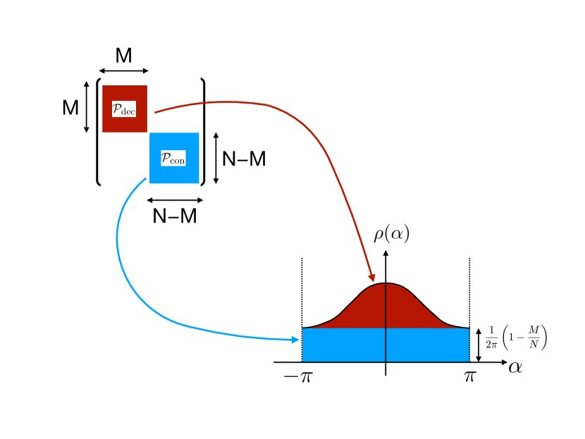
Here, 𝒫consubscript𝒫con\mathcal{P}_{\rm con} can be any element of SU(NM𝑁𝑀N-M), and the generic phase distribution in this part is uniform in the limit of NM𝑁𝑀N-M\to\infty. The phases of 𝒫decsubscript𝒫dec\mathcal{P}_{\rm dec} and 𝒫consubscript𝒫con\mathcal{P}_{\rm con} are α1,,αMsubscript𝛼1subscript𝛼𝑀\alpha_{1},\cdots,\alpha_{M} and αM+1,,αNsubscript𝛼𝑀1subscript𝛼𝑁\alpha_{M+1},\cdots,\alpha_{N}, respectively. From these, we can determine the distribution of the phases ρdec(α)subscript𝜌dec𝛼\rho_{\rm dec}(\alpha) and ρcon(α)subscript𝜌con𝛼\rho_{\rm con}(\alpha). The latter is constant,

ρcon(α)=12π,subscript𝜌con𝛼12𝜋\displaystyle\rho_{\rm con}(\alpha)=\frac{1}{2\pi}\,, (60)

while the former is not and its smallest value is zero. For the model under consideration, we can fix center symmetry in such a way that

ρdec(±π)=0.subscript𝜌decplus-or-minus𝜋0\displaystyle\rho_{\rm dec}(\pm\pi)=0\,. (61)

The full distribution is

ρ(α)𝜌𝛼\displaystyle\rho(\alpha) =(1MN)ρcon(α)+MNρdec(α)absent1𝑀𝑁subscript𝜌con𝛼𝑀𝑁subscript𝜌dec𝛼\displaystyle=\left(1-\frac{M}{N}\right)\cdot\rho_{\rm con}(\alpha)+\frac{M}{N}\cdot\rho_{\rm dec}(\alpha)
=12π(1MN)+MNρdec(α).absent12𝜋1𝑀𝑁𝑀𝑁subscript𝜌dec𝛼\displaystyle=\frac{1}{2\pi}\cdot\left(1-\frac{M}{N}\right)+\frac{M}{N}\cdot\rho_{\rm dec}(\alpha)\,. (62)

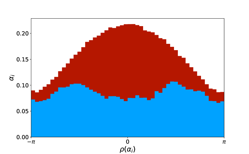
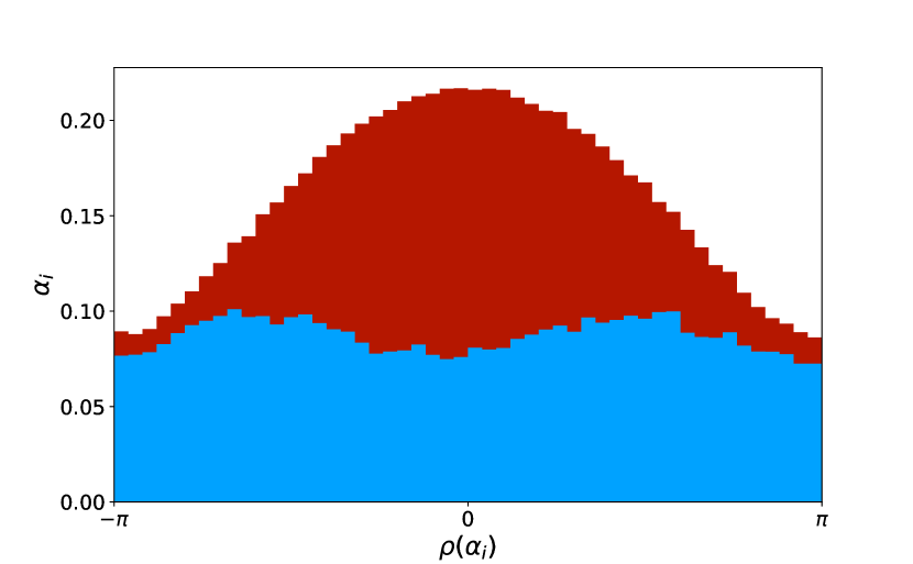
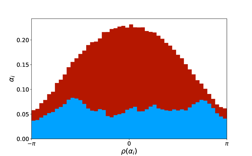
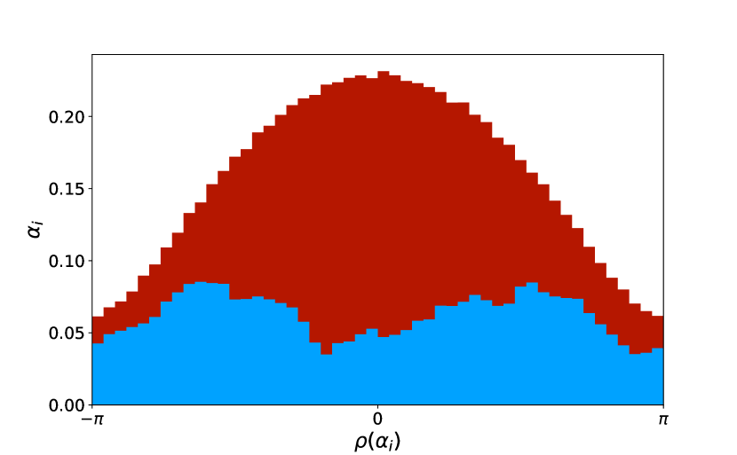
See Fig. 3. Constrained simulation of the second kind enforces this separation by constraining Pdecsubscript𝑃decP_{\rm dec} to be the appropriate value for each M𝑀M and setting Pconsubscript𝑃conP_{\rm con} to be zero. In the large-N𝑁N limit, this is equivalent to the constrained simulation of the first kind plus sorting of the phases, because the distribution becomes continuous and sample-by-sample fluctuation is suppressed.
Refer to caption
Figure 3: Sketches of the distribution of the phases of Polyakov loop in the partially-deconfined phase. Constant offset comes from the confined Polyakov loop 𝒫consubscript𝒫con\mathcal{P}_{\rm con} while the non-uniform part comes from the deconfined Polyakov loop 𝒫decsubscript𝒫dec\mathcal{P}_{\rm dec}.

For our numerical analysis via the Euclidean path integral, we prefer the Polyakov loop to have the form (59) at any Euclidean time t𝑡t so that the SU(M𝑀M)-deconfined sector is always in the upper-left M×M𝑀𝑀M\times M-block. The static diagonal gauge is suitable for this purpose: because the gauge field Atsubscript𝐴𝑡A_{t} is constant, the Polyakov loop does not depend on Euclidean time t𝑡t. (If Atsubscript𝐴𝑡A_{t} is not static, the Polyakov loop can depend on t𝑡t, although the phases do not.) By appropriately fixing the residual SN symmetry, we can have the same embedding visualized in Fig. 1 at any t𝑡t.

The model under consideration has a first-order confinement/deconfinement transition around Tc=12log(2d1)subscript𝑇𝑐122𝑑1T_{c}=\frac{1}{2\log(2d-1)} Hanada:2014noa . It is easy to see the two-state signal when N𝑁N is not too large. When N𝑁N is large, we can see one of two phases depending on the initial configuration for the simulation.

In order to determine the size of deconfined sector for each N𝑁N, let us take P𝑃P to be real and positive (i.e., P=|P|𝑃𝑃P=|P|) configuration-by-configuration, by using the U(1) center symmetry. For each fixed value of P𝑃P, we collect many samples to determine the distribution of the phases α𝛼\alpha, denoted by ρ(α)𝜌𝛼\rho(\alpha). Because of (61) and (62), the minimum value of ρ(α)𝜌𝛼\rho(\alpha) (which should be at α=±π𝛼plus-or-minus𝜋\alpha=\pm\pi) is related to the size of the deconfined sector M𝑀M by Hanada:2020uvt

ρ(±π)=12π(1MN).𝜌plus-or-minus𝜋12𝜋1𝑀𝑁\displaystyle\rho(\pm\pi)=\frac{1}{2\pi}\left(1-\frac{M}{N}\right).

Note that this relation is precise in the large-N𝑁N limit. After determining M𝑀M for each P𝑃P and N𝑁N, we can perform the constrained simulation of the second kind with Pdec=NNMP(M)subscript𝑃dec𝑁𝑁𝑀𝑃𝑀P_{\rm dec}=\frac{N}{N-M}P(M).

The constrained-simulation methods in this paper are essentially the same as the one used in Ref. Watanabe:2020ufk . The only difference is that the models studied in Ref. Watanabe:2020ufk had the simpler relation P=M2N𝑃𝑀2𝑁P=\frac{M}{2N}, which does not hold in the model under consideration in this paper. Therefore, we must determine the relationship between P𝑃P and M𝑀M by numerically determining ρ(±π)𝜌plus-or-minus𝜋\rho(\pm\pi) in the constrained simulation of the first kind.

In general, ρ(α)𝜌𝛼\rho(\alpha) can be written as

ρ(α)=12π+k=1ρ~kcos(kα).𝜌𝛼12𝜋superscriptsubscript𝑘1subscript~𝜌𝑘𝑘𝛼\displaystyle\rho(\alpha)=\frac{1}{2\pi}+\sum_{k=1}^{\infty}\tilde{\rho}_{k}\cos(k\alpha). (63)

We determine the coefficients ρ~ksubscript~𝜌𝑘\tilde{\rho}_{k} based on the simulation data, by using a Bayesian inference procedure with the likelihood of the data α𝛼\alpha given by Eq. (63).

Each of the nconfigsubscript𝑛confign_{\rm config} configurations contains N𝑁N phases α1,,αNsubscript𝛼1subscript𝛼𝑁\alpha_{1},\cdots,\alpha_{N}. Following the usual assumption of the self-averaging nature, i.e., the phase distribution does not depend on samples for sufficiently large N𝑁N, we suppose that each αisubscript𝛼𝑖\alpha_{i} is obtained with a probability ρ(αi)𝜌subscript𝛼𝑖\rho(\alpha_{i}), regardless of the values of the other phases. Then, for a given model distribution ρ(α)𝜌𝛼\rho(\alpha) specified by a fixed set of coefficients {ρ~k}subscript~𝜌𝑘\{\tilde{\rho}_{k}\}, the probability that {α}=(α1,,αN)𝛼subscript𝛼1subscript𝛼𝑁\{\alpha\}=(\alpha_{1},\cdots,\alpha_{N}) is obtained is simply the product of the individual phases probabilities:

i=1Nρ(αi).superscriptsubscriptproduct𝑖1𝑁𝜌subscript𝛼𝑖\displaystyle\prod_{i=1}^{N}\rho(\alpha_{i}). (64)

Taking into account all configurations (assumed to be independent), we obtain the likelihood function for the data {α}𝛼\{\alpha\}, given the parameters {ρ~k}subscript~𝜌𝑘\{\tilde{\rho}_{k}\}:

L({α(1)},,{α(nconfig)}|{ρ~k})=n=1nconfigi=1Nρ(αi(n)).𝐿superscript𝛼1conditionalsuperscript𝛼subscript𝑛configsubscript~𝜌𝑘superscriptsubscriptproduct𝑛1subscript𝑛configsuperscriptsubscriptproduct𝑖1𝑁𝜌superscriptsubscript𝛼𝑖𝑛\displaystyle L(\{\alpha^{(1)}\},\cdots,\{\alpha^{(n_{\rm config})}\}|\{\tilde{\rho}_{k}\})=\prod_{n=1}^{n_{\rm config}}\prod_{i=1}^{N}\rho(\alpha_{i}^{(n)}). (65)

We use Bayes rule to compute the posterior distribution over the parameters {ρ~k}subscript~𝜌𝑘\{\tilde{\rho}_{k}\} given a set of observations corresponding to the data {α(1)},,{α(nconfig)}superscript𝛼1superscript𝛼subscript𝑛config\{\alpha^{(1)}\},\cdots,\{\alpha^{(n_{\rm config})}\}. In practice, we need to truncate the Fourier expansion in Eq. (63) at some order ΛΛ\Lambda, setting ρ~k=0subscript~𝜌𝑘0\tilde{\rho}_{k}=0 for k>Λ𝑘Λk>\Lambda, and we choose a uniform prior distribution centered around zero and with bounds ±0.1plus-or-minus0.1\pm 0.1. At fixed order ΛΛ\Lambda we compute the posterior over exactly ΛΛ\Lambda parameters by using a dynamical Nested Sampling algorithm skilling2004nested ; Buchner2021nestedsampling implemented in the python library ultranest Buchner2021ultranest .

Ultimately, we do not care about the values of the model parameters {ρ~k}subscript~𝜌𝑘\{\tilde{\rho}_{k}\}, but we want to use their posterior distribution to sample all models ρ(α)𝜌𝛼\rho(\alpha) that are compatible with the data. With these samples we have direct access to the expectation value of ρ(π)=12π(1MN)𝜌𝜋12𝜋1𝑀𝑁\rho(\pi)=\frac{1}{2\pi}\left(1-\frac{M}{N}\right), hence to the expectation value of M𝑀M and its corresponding error bar, given by the 161616% and 848484% quantiles of the posterior predictive distribution.

We tried a few different values of the Fourier expansion order ΛΛ\Lambda and found that results are consistent within error bars for Λ{2,3,4,5}Λ2345\Lambda\in\{2,3,4,5\}. For our analysis we choose to consider Λ=3Λ3\Lambda=3 out of simplicity.

The values of M𝑀M for T=0.29𝑇0.29T=0.29 obtained this way are summarized in Table 1. For each fixed N𝑁N and P𝑃P, there is a weak dependence on the lattice size ntsubscript𝑛𝑡n_{t}.

P𝑃P N𝑁N ntsubscript𝑛𝑡n_{t} M𝑀M
0.2 16 16 7.440.11+0.12subscriptsuperscript7.440.120.117.44^{+0.12}_{-0.11}
24 7.620.16+0.15subscriptsuperscript7.620.150.167.62^{+0.15}_{-0.16}
32 7.560.12+0.11subscriptsuperscript7.560.110.127.56^{+0.11}_{-0.12}
24 16 10.990.18+0.18subscriptsuperscript10.990.180.1810.99^{+0.18}_{-0.18}
24 11.130.19+0.19subscriptsuperscript11.130.190.1911.13^{+0.19}_{-0.19}
32 11.120.22+0.22subscriptsuperscript11.120.220.2211.12^{+0.22}_{-0.22}
32 16 14.510.19+0.21subscriptsuperscript14.510.210.1914.51^{+0.21}_{-0.19}
24 14.770.22+0.22subscriptsuperscript14.770.220.2214.77^{+0.22}_{-0.22}
32 14.910.23+0.21subscriptsuperscript14.910.210.2314.91^{+0.21}_{-0.23}
64 16 28.700.31+0.31subscriptsuperscript28.700.310.3128.70^{+0.31}_{-0.31}
24 29.040.34+0.31subscriptsuperscript29.040.310.3429.04^{+0.31}_{-0.34}
32 29.060.29+0.29subscriptsuperscript29.060.290.2929.06^{+0.29}_{-0.29}
96 16 42.780.38+0.40subscriptsuperscript42.780.400.3842.78^{+0.40}_{-0.38}
24 43.190.49+0.48subscriptsuperscript43.190.480.4943.19^{+0.48}_{-0.49}
0.25 16 16 10.060.10+0.09subscriptsuperscript10.060.090.1010.06^{+0.09}_{-0.10}
24 9.990.13+0.13subscriptsuperscript9.990.130.139.99^{+0.13}_{-0.13}
32 10.180.15+0.14subscriptsuperscript10.180.140.1510.18^{+0.14}_{-0.15}
24 16 14.850.16+0.17subscriptsuperscript14.850.170.1614.85^{+0.17}_{-0.16}
24 14.920.17+0.17subscriptsuperscript14.920.170.1714.92^{+0.17}_{-0.17}
32 15.180.12+0.11subscriptsuperscript15.180.110.1215.18^{+0.11}_{-0.12}
32 16 19.520.15+0.18subscriptsuperscript19.520.180.1519.52^{+0.18}_{-0.15}
24 19.810.23+0.22subscriptsuperscript19.810.220.2319.81^{+0.22}_{-0.23}
32 19.920.18+0.19subscriptsuperscript19.920.190.1819.92^{+0.19}_{-0.18}
64 16 38.190.28+0.30subscriptsuperscript38.190.300.2838.19^{+0.30}_{-0.28}
24 38.770.36+0.37subscriptsuperscript38.770.370.3638.77^{+0.37}_{-0.36}
32 39.110.34+0.33subscriptsuperscript39.110.330.3439.11^{+0.33}_{-0.34}
96 16 56.500.34+0.35subscriptsuperscript56.500.350.3456.50^{+0.35}_{-0.34}
24 57.430.40+0.42subscriptsuperscript57.430.420.4057.43^{+0.42}_{-0.40}
Table 1: P𝑃P vs M𝑀M at T=0.29𝑇0.29T=0.29. The central value of M𝑀M is the median of the posterior predictive distribution. The lower and upper bound are the 161616% and 848484% quantiles, respectively.
P𝑃P N𝑁N M𝑀M at T=0.29𝑇0.29T=0.29 M𝑀M at T=0.30𝑇0.30T=0.30 M𝑀M at T=0.31𝑇0.31T=0.31
0.2 16 7.620.16+0.15subscriptsuperscript7.620.150.167.62^{+0.15}_{-0.16} 7.750.15+0.15subscriptsuperscript7.750.150.157.75^{+0.15}_{-0.15} 7.830.16+0.16subscriptsuperscript7.830.160.167.83^{+0.16}_{-0.16}
24 11.130.19+0.19subscriptsuperscript11.130.190.1911.13^{+0.19}_{-0.19} 11.310.20+0.19subscriptsuperscript11.310.190.2011.31^{+0.19}_{-0.20} 11.680.20+0.19subscriptsuperscript11.680.190.2011.68^{+0.19}_{-0.20}
32 14.770.22+0.22subscriptsuperscript14.770.220.2214.77^{+0.22}_{-0.22} 15.030.20+0.20subscriptsuperscript15.030.200.2015.03^{+0.20}_{-0.20} 15.230.22+0.22subscriptsuperscript15.230.220.2215.23^{+0.22}_{-0.22}
0.25 16 9.990.13+0.13subscriptsuperscript9.990.130.139.99^{+0.13}_{-0.13} 10.360.14+0.15subscriptsuperscript10.360.150.1410.36^{+0.15}_{-0.14} 10.590.14+0.14subscriptsuperscript10.590.140.1410.59^{+0.14}_{-0.14}
24 14.920.17+0.17subscriptsuperscript14.920.170.1714.92^{+0.17}_{-0.17} 15.610.16+0.17subscriptsuperscript15.610.170.1615.61^{+0.17}_{-0.16} 15.950.17+0.16subscriptsuperscript15.950.160.1715.95^{+0.16}_{-0.17}
32 19.810.23+0.22subscriptsuperscript19.810.220.2319.81^{+0.22}_{-0.23} 20.500.16+0.18subscriptsuperscript20.500.180.1620.50^{+0.18}_{-0.16} 21.070.19+0.20subscriptsuperscript21.070.200.1921.07^{+0.20}_{-0.19}
Table 2: P𝑃P vs M𝑀M at three different temperatures for nt=24subscript𝑛𝑡24n_{t}=24. The central value of M𝑀M is the median of the posterior predictive distribution. The lower and upper bound are the 161616% and 848484% quantiles, respectively.

In this paper, we are trying to study the partially-deconfined saddle. The temperature of the saddle changes slightly with P𝑃P, while we varied P𝑃P at fixed T𝑇T. We are implicitly assuming that a slight difference of temperature does not have a significant effect if P𝑃P is fixed. The validity of this assumption requires that the saddle is insensitive with respect to the temperature. To test this, we looked at the value of M𝑀M for different values of temperature at fixed P𝑃P. See Table 2 for the relation between P𝑃P and M𝑀M for T=0.29,0.30𝑇0.290.30T=0.29,0.30 and T=0.31𝑇0.31T=0.31. The dependence on temperature is rather mild (mostly compatible within error bars). Hence, we assume other quantities such as the string tension are not sensitive to the small change of temperature. We leave an explicit confirmation of this assumption as a future work.

5 Flux tube in partially-deconfined phase

5.1 Theoretical expectations

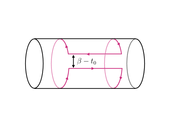
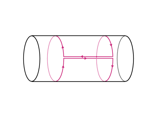
In this section, we demonstrate (3) and (4) using Eguchi-Kawai equivalence. The Eguchi-Kawai model is easier for numerical purposes, but the lack of the spatial dimensions forces us to rewrite the two-point functions on the left-hand side of (3) and (4) to slightly different forms. We define the temporal Wilson loop with temporal extent 0<t0β0subscript𝑡0𝛽0<t_{0}\leq\beta and spatial extent L𝐿L in the lattice unit, as shown in See Fig. 4. When t0=βsubscript𝑡0𝛽t_{0}=\beta (Fig. 5), it is equivalent to the two-point function of the Polyakov loop, as we will see shortly. Thanks to Eguchi-Kawai equivalence, we can calculate this Wilson loop by using the Eguchi-Kawai model.
Refer to caption
Figure 4: The temporal Wilson loop Wμ(L,t0)subscript𝑊𝜇𝐿subscript𝑡0W_{\mu}(L,t_{0}) considered in this work. A spatial Wilson line with length L𝐿L is created, goes through Euclidean time evolution around the temporal circle, and is then annihilated. By exchanging the role of time and space, we can interpret this also as the propagation of an open string along the compactified space over Euclidean time L𝐿L. We will focus on the case of t0=βsubscript𝑡0𝛽t_{0}=\beta.
Refer to caption
Figure 5: Temporal Wilson loop Wμ(L,β)subscript𝑊𝜇𝐿𝛽W_{\mu}(L,\beta). Such a Wilson loop is equivalent to the two-point function of Polyakov loops.

Let us elucidate the physical meaning of this loop. Let Fsuperscript𝐹F^{\dagger} be a creation operator for two heavy probe particles ϕitalic-ϕ\phi and χ𝜒\chi connected by a Wilson line Nair:2005iw ,

F^μ(x,L)=ϕ^a(x)U^μ,ab(x,x+Lμ^)χ^b(x+Lμ^).superscriptsubscript^𝐹𝜇𝑥𝐿subscriptsuperscript^italic-ϕ𝑎𝑥subscript^𝑈𝜇𝑎𝑏𝑥𝑥𝐿^𝜇superscriptsubscript^𝜒𝑏𝑥𝐿^𝜇\displaystyle\hat{F}_{\mu}^{\dagger}(\vec{x},L)=\hat{\phi}^{\dagger}_{a}(\vec{x})\hat{U}_{\mu,ab}(\vec{x},\vec{x}+L\hat{\mu})\hat{\chi}_{b}^{\dagger}(\vec{x}+L\hat{\mu}). (66)

Then Wμ(L,t0)subscript𝑊𝜇𝐿subscript𝑡0W_{\mu}(L,t_{0}) is

Wμ(L,t0)subscript𝑊𝜇𝐿subscript𝑡0\displaystyle W_{\mu}(L,t_{0}) =1Z(β)iEi|e(βt0)H^F^μet0H^F^μ|Eiabsent1𝑍𝛽subscript𝑖quantum-operator-productsubscript𝐸𝑖superscript𝑒𝛽subscript𝑡0^𝐻subscript^𝐹𝜇superscript𝑒subscript𝑡0^𝐻subscriptsuperscript^𝐹𝜇subscript𝐸𝑖\displaystyle=\frac{1}{Z(\beta)}\sum_{i}\left\langle E_{i}\right|e^{-(\beta-t_{0})\hat{H}}\hat{F}_{\mu}e^{-t_{0}\hat{H}}\hat{F}^{\dagger}_{\mu}\left|E_{i}\right\rangle
=1Z(β)ieβEiEi|F^μet0(H^Ei)F^μ|Ei.absent1𝑍𝛽subscript𝑖superscript𝑒𝛽subscript𝐸𝑖quantum-operator-productsubscript𝐸𝑖subscript^𝐹𝜇superscript𝑒subscript𝑡0^𝐻subscript𝐸𝑖subscriptsuperscript^𝐹𝜇subscript𝐸𝑖\displaystyle=\frac{1}{Z(\beta)}\sum_{i}e^{-\beta E_{i}}\left\langle E_{i}\right|\hat{F}_{\mu}e^{-t_{0}(\hat{H}-E_{i})}\hat{F}^{\dagger}_{\mu}\left|E_{i}\right\rangle. (67)

Note that the contribution from the mass of the probes is subtracted.

Let us write Fμ|Eisubscriptsuperscript𝐹𝜇ketsubscript𝐸𝑖F^{\dagger}_{\mu}\left|E_{i}\right\rangle as a linear combination of the energy eigenstates,

F^μ|Ei=jcij|Ej.subscriptsuperscript^𝐹𝜇ketsubscript𝐸𝑖subscript𝑗subscript𝑐𝑖𝑗ketsubscript𝐸𝑗\displaystyle\hat{F}^{\dagger}_{\mu}\left|E_{i}\right\rangle=\sum_{j}c_{ij}\left|E_{j}\right\rangle. (68)

Then,

Wμ(L,t0)=1Z(β)i,jeβEi|cij|2et0(EjEi).subscript𝑊𝜇𝐿subscript𝑡01𝑍𝛽subscript𝑖𝑗superscript𝑒𝛽subscript𝐸𝑖superscriptsubscript𝑐𝑖𝑗2superscript𝑒subscript𝑡0subscript𝐸𝑗subscript𝐸𝑖\displaystyle W_{\mu}(L,t_{0})=\frac{1}{Z(\beta)}\sum_{i,j}e^{-\beta E_{i}}|c_{ij}|^{2}e^{-t_{0}(E_{j}-E_{i})}. (69)

Suppose the sum over all the states can be replaced by a typical energy eigenstate |Eiketsubscript𝐸𝑖|E_{i}\rangle. Then,

Wμ(L,t0)j|cij|2et0(EjEi).similar-tosubscript𝑊𝜇𝐿subscript𝑡0subscript𝑗superscriptsubscript𝑐𝑖𝑗2superscript𝑒subscript𝑡0subscript𝐸𝑗subscript𝐸𝑖\displaystyle W_{\mu}(L,t_{0})\sim\sum_{j}|c_{ij}|^{2}e^{-t_{0}(E_{j}-E_{i})}. (70)

If the minimum excitation above Eisubscript𝐸𝑖E_{i} increases linearly with L𝐿L, we have Wμ(L,t0)ecLsimilar-tosubscript𝑊𝜇𝐿subscript𝑡0superscript𝑒𝑐𝐿W_{\mu}(L,t_{0})\sim e^{-cL}, with some constant c𝑐c. We expect this to happen in the confined sector, i.e., we expect Wμ,con(L,t0)ecLsimilar-tosubscript𝑊𝜇con𝐿subscript𝑡0superscript𝑒𝑐𝐿W_{\mu,{\rm con}}(L,t_{0})\sim e^{-cL}. If only the low-energy states contribute, we should have ct0σproportional-to𝑐subscript𝑡0𝜎c\propto t_{0}\sigma, where σ𝜎\sigma is called the string tension. In the Eguchi-Kawai model, by using the Polyakov line

𝒫diag(eiα1,,eiαN),𝒫diagsuperscript𝑒𝑖subscript𝛼1superscript𝑒𝑖subscript𝛼𝑁\displaystyle{\cal P}\equiv{\rm diag}(e^{i\alpha_{1}},\cdots,e^{i\alpha_{N}}), (71)

we can write Wμ(L,β)subscript𝑊𝜇𝐿𝛽W_{\mu}(L,\beta) as

Wμ(L,β)=Tr(𝒫(Uμ(t))L𝒫(Uμ(t))L).subscript𝑊𝜇𝐿𝛽delimited-⟨⟩Tr𝒫superscriptsubscript𝑈𝜇𝑡𝐿superscript𝒫superscriptsubscript𝑈𝜇superscript𝑡𝐿\displaystyle W_{\mu}(L,\beta)=\left\langle{\rm Tr}\left({\cal P}(U_{\mu}(t))^{L}{\cal P}^{\dagger}(U_{\mu}(t)^{\dagger})^{L}\right)\right\rangle. (72)

We can see the exponential decay of Wμ(L,β)subscript𝑊𝜇𝐿𝛽W_{\mu}(L,\beta) in Fig. 6 for the completely-confined case.

1NWμ(L,β)1𝑁subscript𝑊𝜇𝐿𝛽\frac{1}{N}W_{\mu}(L,\beta) is equivalent to the two-point function of Polyakov loops, i.e.,

1NWμ(L,β)=Tr𝒫(x)Tr𝒫(x+Lμ^).1𝑁subscript𝑊𝜇𝐿𝛽delimited-⟨⟩Tr𝒫𝑥Tr𝒫𝑥𝐿^𝜇\displaystyle\frac{1}{N}W_{\mu}(L,\beta)=\left\langle{\rm Tr}{\cal P}(\vec{x})\cdot{\rm Tr}{\cal P}(\vec{x}+L\hat{\mu})\right\rangle. (73)

Here μ^^𝜇\hat{\mu} is the unit vector along the μ𝜇\mu-th dimension. One way to see this is to exchange the roles of temporal and spatial directions. Namely, we interpret the μ𝜇\mu-direction to be imaginary time. Wμ(L,t0)subscript𝑊𝜇𝐿subscript𝑡0W_{\mu}(L,t_{0}) is interpreted as the propagation along the imaginary time direction of an open string with length t0subscript𝑡0t_{0} stretched along the spatial circle with circumference β𝛽\beta. When t0=βsubscript𝑡0𝛽t_{0}=\beta and the color factors (Chan-Paton factors) at the endpoints of the open string are summed over, we get a closed string, or equivalently, the Polyakov loop.

To see the properties of the confined and deconfined sectors separately, we define the Polyakov line in the deconfined sector,

𝒫decdiag(eiα1,,eiαM,0,,0),subscript𝒫decdiagsuperscript𝑒𝑖subscript𝛼1superscript𝑒𝑖subscript𝛼𝑀00\displaystyle{\cal P}_{\rm dec}\equiv{\rm diag}(e^{i\alpha_{1}},\cdots,e^{i\alpha_{M}},0,\cdots,0), (74)

and that in the confined sector,

𝒫condiag(0,,0,eiαM+1,,eiαN).subscript𝒫condiag00superscript𝑒𝑖subscript𝛼𝑀1superscript𝑒𝑖subscript𝛼𝑁\displaystyle{\cal P}_{\rm con}\equiv{\rm diag}(0,\cdots,0,e^{i\alpha_{M+1}},\cdots,e^{i\alpha_{N}}). (75)

By using these, we can define the counterparts of two-point functions in the lattice gauge theory 𝒫dec(x)𝒫dec(y)delimited-⟨⟩subscript𝒫dec𝑥subscript𝒫dec𝑦\left\langle{\cal P}_{\rm dec}(\vec{x}){\cal P}_{\rm dec}(\vec{y})\right\rangle, 𝒫con(x)𝒫con(y)delimited-⟨⟩subscript𝒫con𝑥subscript𝒫con𝑦\left\langle{\cal P}_{\rm con}(\vec{x}){\cal P}_{\rm con}(\vec{y})\right\rangle and 𝒫con(x)𝒫dec(y)delimited-⟨⟩subscript𝒫con𝑥subscript𝒫dec𝑦\left\langle{\cal P}_{\rm con}(\vec{x}){\cal P}_{\rm dec}(\vec{y})\right\rangle as

Wμ,dec(L,β)Tr(𝒫dec(Uμ(t))L𝒫dec(Uμ(t))L),subscript𝑊𝜇dec𝐿𝛽delimited-⟨⟩Trsubscript𝒫decsuperscriptsubscript𝑈𝜇𝑡𝐿superscriptsubscript𝒫decsuperscriptsubscript𝑈𝜇superscript𝑡𝐿\displaystyle W_{\mu,{\rm dec}}(L,\beta)\equiv\left\langle{\rm Tr}\left({\cal P}_{\rm dec}(U_{\mu}(t))^{L}{\cal P}_{\rm dec}^{\dagger}(U_{\mu}(t)^{\dagger})^{L}\right)\right\rangle, (76)
Wμ,con(L,β)Tr(𝒫con(Uμ(t))L𝒫con(Uμ(t))L).subscript𝑊𝜇con𝐿𝛽delimited-⟨⟩Trsubscript𝒫consuperscriptsubscript𝑈𝜇𝑡𝐿superscriptsubscript𝒫consuperscriptsubscript𝑈𝜇superscript𝑡𝐿\displaystyle W_{\mu,{\rm con}}(L,\beta)\equiv\left\langle{\rm Tr}\left({\cal P}_{\rm con}(U_{\mu}(t))^{L}{\cal P}_{\rm con}^{\dagger}(U_{\mu}(t)^{\dagger})^{L}\right)\right\rangle. (77)

and

Wμ,mix(L,β)Tr(𝒫con(Uμ(t))L𝒫dec(Uμ(t))L).subscript𝑊𝜇mix𝐿𝛽delimited-⟨⟩Trsubscript𝒫consuperscriptsubscript𝑈𝜇𝑡𝐿superscriptsubscript𝒫decsuperscriptsubscript𝑈𝜇superscript𝑡𝐿\displaystyle W_{\mu,{\rm mix}}(L,\beta)\equiv\left\langle{\rm Tr}\left({\cal P}_{\rm con}(U_{\mu}(t))^{L}{\cal P}_{\rm dec}^{\dagger}(U_{\mu}(t)^{\dagger})^{L}\right)\right\rangle. (78)

We can also define Wμ,dec(L,t0)subscript𝑊𝜇dec𝐿subscript𝑡0W_{\mu,{\rm dec}}(L,t_{0}), Wμ,con(L,t0)subscript𝑊𝜇con𝐿subscript𝑡0W_{\mu,{\rm con}}(L,t_{0}) and Wμ,mix(L,t0)subscript𝑊𝜇mix𝐿subscript𝑡0W_{\mu,{\rm mix}}(L,t_{0}) in a similar manner.

Because 1NWμ(L,β)1𝑁subscript𝑊𝜇𝐿𝛽\frac{1}{N}W_{\mu}(L,\beta) is equivalent to the two-point function of Polyakov loops, and because the connected part of the two-point function is suppressed at long distance (L𝐿L\to\infty), we will have

limL1NWμ(L,β)=|P|2.subscript𝐿1𝑁subscript𝑊𝜇𝐿𝛽superscriptdelimited-⟨⟩𝑃2\displaystyle\lim_{L\to\infty}\frac{1}{N}W_{\mu}(L,\beta)=|\langle P\rangle|^{2}. (79)

We expect Wμ,con(L,β)subscript𝑊𝜇con𝐿𝛽W_{\mu,{\rm con}}(L,\beta) and Wμ,mix(L,β)subscript𝑊𝜇mix𝐿𝛽W_{\mu,{\rm mix}}(L,\beta) to vanish at large L𝐿L, and hence we expect

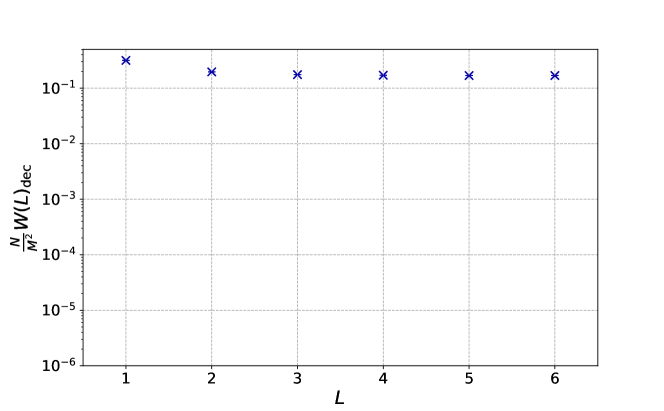
limL1NWμ,dec(L,β)=|P|2.subscript𝐿1𝑁subscript𝑊𝜇dec𝐿𝛽superscriptdelimited-⟨⟩𝑃2\displaystyle\lim_{L\to\infty}\frac{1}{N}W_{\mu,{\rm dec}}(L,\beta)=|\langle P\rangle|^{2}. (80)

We expect that Wμ,con(L,β)subscript𝑊𝜇con𝐿𝛽W_{\mu,{\rm con}}(L,\beta) and Wμ,mix(L,β)subscript𝑊𝜇mix𝐿𝛽W_{\mu,{\rm mix}}(L,\beta) vanish in a very specific manner. We expect the exponential decay at long distance with the same string tension as the confined sector, i.e., we expect

1NWμ,con(L,β)=Ccon(N,M)exp(σLβ)1𝑁subscript𝑊𝜇con𝐿𝛽subscript𝐶con𝑁𝑀𝜎𝐿𝛽\displaystyle\frac{1}{N}W_{\mu,{\rm con}}(L,\beta)=C_{\rm con}(N,M)\cdot\exp\left(-\sigma L\beta\right) (81)

and

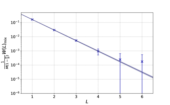
1NWμ,mix(L,β)=Cmix(N,M)exp(σLβ).1𝑁subscript𝑊𝜇mix𝐿𝛽subscript𝐶mix𝑁𝑀𝜎𝐿𝛽\displaystyle\frac{1}{N}W_{\mu,{\rm mix}}(L,\beta)=C_{\rm mix}(N,M)\cdot\exp\left(-\sigma L\beta\right)\ . (82)

To obtain (82), we can interpret the μ𝜇\mu-direction to be the Euclidean time. Then, closed string in the confined sector is created by 𝒫consubscript𝒫con\mathcal{P}_{\rm con} and propagate distance L𝐿L. Then it is annihilated by 𝒫decsubscript𝒫dec\mathcal{P}_{\rm dec}. It is natural to expect that 𝒫decsubscript𝒫dec\mathcal{P}_{\rm dec} contains a small but nonzero contribution from the lightest mode in 𝒫consubscript𝒫con\mathcal{P}_{\rm con} because there is no reason that it is forbidden, and hence, we expect to see the propagation of the closed string in the confined sector that is associated with the decay factor exp(σLβ)𝜎𝐿𝛽\exp\left(-\sigma L\beta\right).

In the strong-coupling lattice gauge theory, with our normalization,

σ=12.𝜎12\displaystyle\sigma=\frac{1}{2}. (83)

Note that the large-N𝑁N limit should be taken first. Approximately, we expect Ccon(N,M)(1MN)2similar-to-or-equalssubscript𝐶con𝑁𝑀superscript1𝑀𝑁2C_{\rm con}(N,M)\simeq\left(1-\frac{M}{N}\right)^{2} and Cmix(N,M)MN(1MN)similar-to-or-equalssubscript𝐶mix𝑁𝑀𝑀𝑁1𝑀𝑁C_{\rm mix}(N,M)\simeq\frac{M}{N}\left(1-\frac{M}{N}\right). To give a stronger constraint on Ccon(N,M)subscript𝐶con𝑁𝑀C_{\rm con}(N,M) and Cmix(N,M)subscript𝐶mix𝑁𝑀C_{\rm mix}(N,M), let us assume that these factors do not depend on the size of the loops along the temporal direction, i.e.,

1NWμ,con(L,t0)=Ccon(N,M)exp(σLt0)1𝑁subscript𝑊𝜇con𝐿subscript𝑡0subscript𝐶con𝑁𝑀𝜎𝐿subscript𝑡0\displaystyle\frac{1}{N}W_{\mu,{\rm con}}(L,t_{0})=C_{\rm con}(N,M)\cdot\exp\left(-\sigma Lt_{0}\right) (84)

and

1NWμ,mix(L,t0)=Cmix(N,M)exp(σLt0).1𝑁subscript𝑊𝜇mix𝐿subscript𝑡0subscript𝐶mix𝑁𝑀𝜎𝐿subscript𝑡0\displaystyle\frac{1}{N}W_{\mu,{\rm mix}}(L,t_{0})=C_{\rm mix}(N,M)\cdot\exp\left(-\sigma Lt_{0}\right)\ . (85)

By definition, the sum of Wμ,con(L,t0=0)subscript𝑊𝜇con𝐿subscript𝑡00W_{\mu,{\rm con}}(L,t_{0}=0) and Wμ,mix(L,t0=0)subscript𝑊𝜇mix𝐿subscript𝑡00W_{\mu,{\rm mix}}(L,t_{0}=0) can be written as

Wμ,con(L,t0=0)+Wμ,mix(L,t0=0)subscript𝑊𝜇con𝐿subscript𝑡00subscript𝑊𝜇mix𝐿subscript𝑡00\displaystyle W_{\mu,{\rm con}}(L,t_{0}=0)+W_{\mu,{\rm mix}}(L,t_{0}=0) =Tr(Πcon(Uμ(t))L1N(Uμ(t))L)absentdelimited-⟨⟩TrsubscriptΠconsuperscriptsubscript𝑈𝜇𝑡𝐿subscript1𝑁superscriptsubscript𝑈𝜇superscript𝑡𝐿\displaystyle=\left\langle{\rm Tr}\left(\Pi_{\rm con}(U_{\mu}(t))^{L}\textbf{1}_{N}(U_{\mu}(t)^{\dagger})^{L}\right)\right\rangle
=Tr(Πcon)absentdelimited-⟨⟩TrsubscriptΠcon\displaystyle=\left\langle{\rm Tr}\left(\Pi_{\rm con}\right)\right\rangle
=NM,absent𝑁𝑀\displaystyle=N-M, (86)

where Πcon=diag(0,,0M,1,,1NM)subscriptΠcondiagsubscript00𝑀subscript11𝑁𝑀\Pi_{\rm con}=\textrm{diag}(\underbrace{0,\cdots,0}_{M},\underbrace{1,\cdots,1}_{N-M}). Therefore,

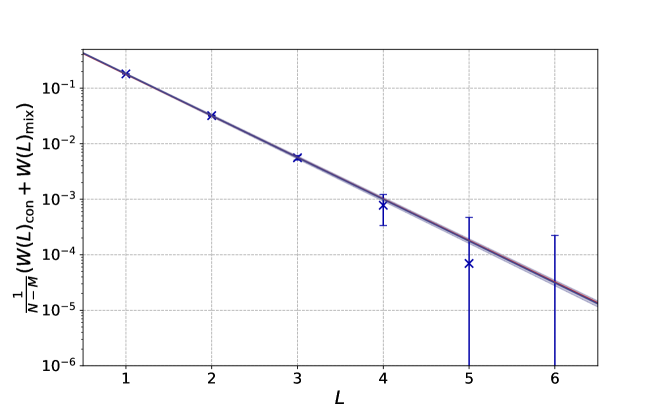
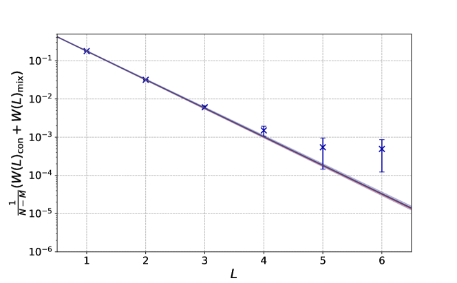
Ccon(N,M)+Cmix(N,M)=1MN,subscript𝐶con𝑁𝑀subscript𝐶mix𝑁𝑀1𝑀𝑁\displaystyle C_{\rm con}(N,M)+C_{\rm mix}(N,M)=1-\frac{M}{N}\ , (87)

if Ccon(N,M)subscript𝐶con𝑁𝑀C_{\rm con}(N,M) and Cmix(N,M)subscript𝐶mix𝑁𝑀C_{\rm mix}(N,M) do not depend on t0subscript𝑡0t_{0}. In Sec. 5.2, we will confirm this relation numerically.

5.2 Simulation results

In this subsection, we will show the simulation results. The expectation values of W(L)𝑊𝐿W(L) used for the analyses are shown in Tables D, D, D, and D.

Completely-confined phase

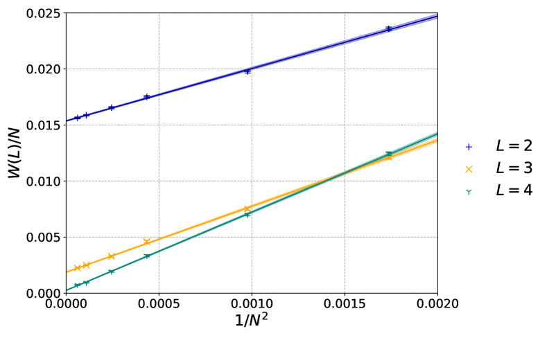
Let us start with the unconstrained simulation at T=0.25𝑇0.25T=0.25, where temperature is sufficiently low such that the completely-confined phase is obtained in the large-N𝑁N limit. We took the lattice size nt=24subscript𝑛𝑡24n_{t}=24, and studied N=16,24,32,48,64,96𝑁162432486496N=16,24,32,48,64,96 and 128128128. We took the average over all spatial dimensions μ=1,2,3𝜇123\mu=1,2,3 and studied W=13μ=13Wμ𝑊13superscriptsubscript𝜇13subscript𝑊𝜇W=\frac{1}{3}\sum_{\mu=1}^{3}W_{\mu}. As we can see in the first panel of Fig. 6, the N𝑁N-dependence of 1NW(L)1𝑁𝑊𝐿\frac{1}{N}W(L) can be fitted well to the fitting ansatz 1NW(L)=a(L)+b(L)N21𝑁𝑊𝐿𝑎𝐿𝑏𝐿superscript𝑁2\frac{1}{N}W(L)=a(L)+\frac{b(L)}{N^{2}}. We used N24𝑁24N\geq 24 to perform the extrapolation to N=𝑁N=\infty. We could achieve reliable extrapolations at L=1,2,3𝐿123L=1,2,3 and 444. For L5𝐿5L\geq 5, larger N𝑁N are needed for reliable extrapolations.

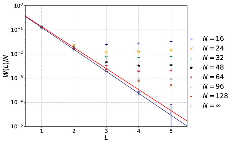
Because the Eguchi-Kawai reduction is valid at N=𝑁N=\infty, we can compare the large-N𝑁N extrapolated values with the theoretical expectation (81) and σ=12𝜎12\sigma=\frac{1}{2}, β=1T=4𝛽1𝑇4\beta=\frac{1}{T}=4, and M=0𝑀0M=0, i.e., 1NW(L,β=4)=exp(2L)1𝑁𝑊𝐿𝛽42𝐿\frac{1}{N}W(L,\beta=4)=\exp(-2L). Note that Ccon(N,M=0)=1subscript𝐶con𝑁𝑀01C_{\rm con}(N,M=0)=1, because of (87) and Cmix(N,M=0)=0subscript𝐶mix𝑁𝑀00C_{\rm mix}(N,M=0)=0. In the second panel of Fig. 6, 1NW(L)1𝑁𝑊𝐿\frac{1}{N}W(L) for each N𝑁N and the large-N𝑁N extrapolation are shown for L=1,2,3,4,5𝐿12345L=1,2,3,4,5. By fitting the large-N𝑁N extrapolated results at 1L41𝐿41\leq L\leq 4 to the ansatz a(L)=exp(cL+d)𝑎𝐿𝑐𝐿𝑑a(L)=\exp(-cL+d), we obtained c=2.0887(30)𝑐2.088730c=2.0887(30) and d=0.0011(31)𝑑0.001131d=0.0011(31). Small deviations from exp(2L)2𝐿\exp(-2L) would be finite-ntsubscript𝑛𝑡n_{t} effects.

Refer to caption
Refer to caption
Figure 6: T=0.25𝑇0.25T=0.25 and nt=24subscript𝑛𝑡24n_{t}=24, without constraint. Temperature is sufficiently low such that the completely-confined phase is realized automatically. For the extrapolation to N=𝑁N=\infty, we used data points at N=24,32,48,64,96,128𝑁2432486496128N=24,32,48,64,96,128 for L=1,2,3,4𝐿1234L=1,2,3,4 and N=48,64,96,128𝑁486496128N=48,64,96,128 for L=5𝐿5L=5. We used the fitting ansatz 1NW(L)=a(L)+b(L)N21𝑁𝑊𝐿𝑎𝐿𝑏𝐿superscript𝑁2\frac{1}{N}W(L)=a(L)+\frac{b(L)}{N^{2}}. By fitting the large-N𝑁N extrapolated results at 1L41𝐿41\leq L\leq 4 by the ansatz a(L)=exp(cL+d)𝑎𝐿𝑐𝐿𝑑a(L)=\exp(-cL+d), we obtained c=2.0887(30)𝑐2.088730c=2.0887(30) and d=0.0011(31)𝑑0.001131d=0.0011(31). This fit is shown by the blue line. The red line is exp(2L)2𝐿\exp(-2L), which is the theoretical expectation for long distance (large L𝐿L) and continuum limit (nt=subscript𝑛𝑡n_{t}=\infty). A small disagreement would be finite-ntsubscript𝑛𝑡n_{t} effects.

We can also probe the confined phase at T=0.29𝑇0.29T=0.29 by constraining P𝑃P to its confined value, P=0𝑃0P=0, as shown in Fig. 7. This is more comparable to the constrained simulation, described below, that we perform at T=0.29𝑇0.29T=0.29 to probe the partial phase, but is here applied to examining the familiar completely-confined phase with its well-established theory and predictions.

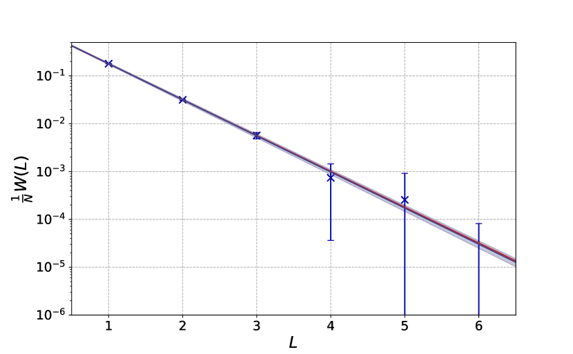
For this, we took the large-N𝑁N and continuum limit at each L𝐿L by performing a weighted least-squares regression with the ansatz 1NWcon(L;nt)=acon(L)+b1,con(L)N2+b2,con(L)nt+b3,con(L)ntN21𝑁subscript𝑊con𝐿subscript𝑛𝑡subscript𝑎con𝐿subscript𝑏1con𝐿superscript𝑁2subscript𝑏2con𝐿subscript𝑛𝑡subscript𝑏3con𝐿subscript𝑛𝑡superscript𝑁2\frac{1}{N}W_{\rm con}(L;n_{t})=a_{\rm con}(L)+\frac{b_{\rm 1,con}(L)}{N^{2}}+\frac{b_{\rm 2,con}(L)}{n_{t}}+\frac{b_{\rm 3,con}(L)}{n_{t}N^{2}}. The weights were derived from the error bars of the Monte-Carlo observables, where the integrated autocorrelation time measured by the Madras-Sokal algorithm Sokal1996MonteCM is taken into account. Then acon(L)subscript𝑎con𝐿a_{\rm con}(L) gives the extrapolated value in the N,nt𝑁subscript𝑛𝑡N,n_{t}\rightarrow\infty limit. Fitting the ansatz acon(L)=exp(cconL+dcon)subscript𝑎con𝐿subscript𝑐con𝐿subscript𝑑cona_{\rm con}(L)=\exp(-c_{\rm con}L+d_{\rm con}), we obtain ccon=1.738(29)subscript𝑐con1.73829c_{\rm con}=1.738(29) and dcon=0.022(31)subscript𝑑con0.02231d_{\rm con}=0.022(31). This is consistent with the theoretical expectation eσβL=e12×0.29Le1.724Lsuperscript𝑒𝜎𝛽𝐿superscript𝑒120.29𝐿similar-to-or-equalssuperscript𝑒1.724𝐿e^{\sigma\beta L}=e^{-\frac{1}{2\times 0.29}L}\simeq e^{-1.724L}.

Refer to caption
Figure 7: T=0.29𝑇0.29T=0.29 with the constraint P=0𝑃0P=0, allowing us to probe the completely-confined phase near the transition. We have extrapolated to the large N𝑁N limit using N=7,10,16,24,32𝑁710162432N=7,10,16,24,32, and to the continuum limit using nt=16,24,32subscript𝑛𝑡162432n_{t}=16,24,32 for each N𝑁N, using the 2D interpolation 1NWcon(L)=acon(L)+b1,con(L)N2+b2,con(L)nt+b3,con(L)ntN21𝑁subscript𝑊con𝐿subscript𝑎con𝐿subscript𝑏1con𝐿superscript𝑁2subscript𝑏2con𝐿subscript𝑛𝑡subscript𝑏3con𝐿subscript𝑛𝑡superscript𝑁2\frac{1}{N}W_{\rm con}(L)=a_{\rm con}(L)+\frac{b_{\rm 1,con}(L)}{N^{2}}+\frac{b_{\rm 2,con}(L)}{n_{t}}+\frac{b_{\rm 3,con}(L)}{n_{t}N^{2}}. We fitted these interpolated values acon(L)subscript𝑎con𝐿a_{\rm con}(L) for 1L41𝐿41\leq L\leq 4 to the ansatz acon(L)=exp(cconL+dcon)subscript𝑎con𝐿subscript𝑐con𝐿subscript𝑑cona_{\rm con}(L)=\exp(-c_{\rm con}L+d_{\rm con}), yielding ccon=1.738(29)subscript𝑐con1.73829c_{\rm con}=1.738(29) and dcon=0.022(31)subscript𝑑con0.02231d_{\rm con}=0.022(31). The fit is shown along with error bounds by the blue line. The theoretical prediction (ccon=1.724subscript𝑐con1.724c_{\rm con}=1.724, and dcon=0subscript𝑑con0d_{\rm con}=0 for M=0𝑀0M=0) is given by the red line, which is mostly obscured by the fit.

Partially-deconfined phase

In Fig. 8, we show Wconsubscript𝑊conW_{\rm con} at T=0.29𝑇0.29T=0.29, P=0.2𝑃0.2P=0.2 and P=0.25𝑃0.25P=0.25, which corresponds to MN0.50similar-to-or-equals𝑀𝑁0.50\frac{M}{N}\simeq 0.50 and MN0.61similar-to-or-equals𝑀𝑁0.61\frac{M}{N}\simeq 0.61. We performed a two-dimensional weighted least-squares regression to take the large N𝑁N and continuum (ntsubscript𝑛𝑡n_{t}\to\infty) limits simultaneously. Note that it is more difficult to take the large-N𝑁N limit at larger L𝐿L, and/or when either M𝑀M or NM𝑁𝑀N-M is small.

Motivated by (81) with Ccon(N,M)(1MN)2similar-to-or-equalssubscript𝐶con𝑁𝑀superscript1𝑀𝑁2C_{\rm con}(N,M)\simeq\left(1-\frac{M}{N}\right)^{2}, we normalized the loop as 1NWcon(L)×(1MN)21𝑁subscript𝑊con𝐿superscript1𝑀𝑁2\frac{1}{N}W_{\rm con}(L)\times\left(1-\frac{M}{N}\right)^{-2}. We will compare the loop normalized this way to eσβL=e12×0.29Le1.724Lsuperscript𝑒𝜎𝛽𝐿superscript𝑒120.29𝐿similar-to-or-equalssuperscript𝑒1.724𝐿e^{\sigma\beta L}=e^{-\frac{1}{2\times 0.29}L}\simeq e^{-1.724L}.

The large-N𝑁N and continuum extrapolations were estimated at each L𝐿L by performing a weighted least-squares regression with the ansatz 1NWcon(L)×(1MN)2=acon(L)+b1,con(L)N(NM)+b2,con(L)nt+b3,con(L)ntN(NM)1𝑁subscript𝑊con𝐿superscript1𝑀𝑁2subscript𝑎con𝐿subscript𝑏1con𝐿𝑁𝑁𝑀subscript𝑏2con𝐿subscript𝑛𝑡subscript𝑏3con𝐿subscript𝑛𝑡𝑁𝑁𝑀\frac{1}{N}W_{\rm con}(L)\times\left(1-\frac{M}{N}\right)^{-2}=a_{\rm con}(L)+\frac{b_{\rm 1,con}(L)}{N(N-M)}+\frac{b_{\rm 2,con}(L)}{n_{t}}+\frac{b_{\rm 3,con}(L)}{n_{t}N(N-M)} 666In the completely-confined phase, we used N2superscript𝑁2N^{2} in the denominators of the regression. For the partial phase, we used N(NM)𝑁𝑁𝑀N(N-M) instead. We found that our data was much closer to being linear in 1N(NM)1𝑁𝑁𝑀\frac{1}{N(N-M)}, both for data points taken at the same P𝑃P but which differed slightly in M/N𝑀𝑁M/N, and also when combining points at different P𝑃P and thus very different values of M/N𝑀𝑁M/N.. Then acon(L)subscript𝑎con𝐿a_{\rm con}(L) gives the extrapolated value of the Wilson loop in the N,nt𝑁subscript𝑛𝑡N,n_{t}\rightarrow\infty limit.

We plotted acon(L)subscript𝑎con𝐿a_{\rm con}(L) in Fig. 8. We can perform one final linear regression with the ansatz log(acon(L))=cconL+dconsubscript𝑎con𝐿subscript𝑐con𝐿subscript𝑑con\log(a_{\rm con}(L))=-c_{\rm con}L+d_{\rm con} to check the area law. Fitting to L4𝐿4L\leq 4, we obtain ccon=1.729(17)subscript𝑐con1.72917c_{\rm con}=1.729(17) and ccon=1.724(23)subscript𝑐con1.72423c_{\rm con}=1.724(23) for P=0.2𝑃0.2P=0.2 and P=0.25𝑃0.25P=0.25, respectively, in good agreement with the theoretical expectation, 1.7241.7241.724. The values of d𝑑d were dcon=0.086(20)subscript𝑑con0.08620d_{\rm con}=0.086(20) and dcon=0.127(28)subscript𝑑con0.12728d_{\rm con}=0.127(28). That they are not zero is not a problem; what we expect instead is (87), which we will confirm shortly.
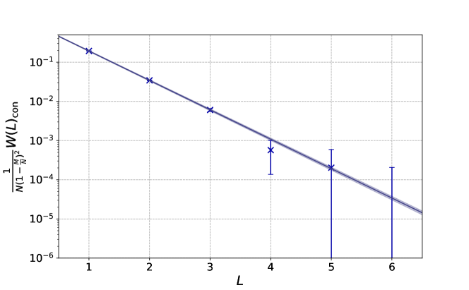
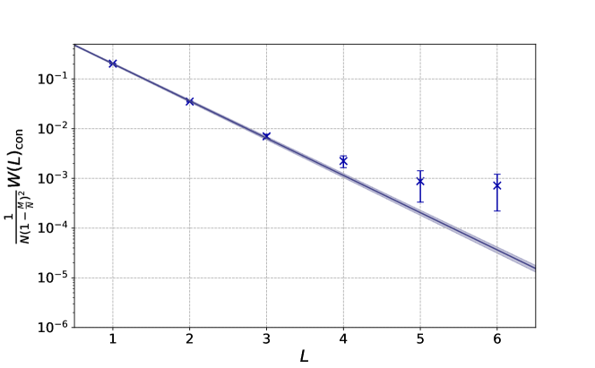
Refer to caption
Refer to caption
Figure 8: Confined subsector Wilson loop, Wconsubscript𝑊conW_{\rm con}, at T=0.29𝑇0.29T=0.29, for P=0.2𝑃0.2P=0.2 and P=0.25𝑃0.25P=0.25, respectively. We have extrapolated to the large N𝑁N limit using N=24,32,64𝑁243264N=24,32,64, and to the continuum limit using nt=16,24,32subscript𝑛𝑡162432n_{t}=16,24,32 for each N𝑁N, using the 2D interpolation 1N(1MN)2Wcon(L)=γcon(L)+β1N2+β2nt+β2ntN21𝑁superscript1𝑀𝑁2subscript𝑊con𝐿subscript𝛾con𝐿subscript𝛽1superscript𝑁2subscript𝛽2subscript𝑛𝑡subscript𝛽2subscript𝑛𝑡superscript𝑁2\frac{1}{N(1-\frac{M}{N})^{2}}W_{\rm con}(L)=\gamma_{\rm con}(L)+\frac{\beta_{1}}{N^{2}}+\frac{\beta_{2}}{n_{t}}+\frac{\beta_{2}}{n_{t}N^{2}}. We fitted these interpolated values γcon(L)subscript𝛾con𝐿\gamma_{\rm con}(L) for 1L41𝐿41\leq L\leq 4 to the ansatz γcon(L)=exp(cconL+dcon)subscript𝛾con𝐿subscript𝑐con𝐿subscript𝑑con\gamma_{\rm con}(L)=\exp(-c_{\rm con}L+d_{\rm con}) and obtained ccon=1.729(17)subscript𝑐con1.72917c_{\rm con}=1.729(17) and ccon=1.724(23)subscript𝑐con1.72423c_{\rm con}=1.724(23) for P=0.2𝑃0.2P=0.2 and P=0.25𝑃0.25P=0.25, respectively. The fit is shown along with error bounds by the blue line.

The mixed-correlator Wmix(L)subscript𝑊mix𝐿W_{\rm mix}(L) is shown in Fig. 9. Motivated by (82) with Cmix(N,M)MN(1MN)similar-to-or-equalssubscript𝐶mix𝑁𝑀𝑀𝑁1𝑀𝑁C_{\rm mix}(N,M)\simeq\frac{M}{N}\left(1-\frac{M}{N}\right), we normalized the loop as 1NWmix(L)×[MN(1MN)]11𝑁subscript𝑊mix𝐿superscriptdelimited-[]𝑀𝑁1𝑀𝑁1\frac{1}{N}W_{\rm mix}(L)\times\left[\frac{M}{N}\left(1-\frac{M}{N}\right)\right]^{-1}. We used a similar process as described for Wconsubscript𝑊conW_{\rm con} above, but using this different normalisation. We find cmix=1.731(21)subscript𝑐mix1.73121c_{\rm mix}=1.731(21) and cmix=1.708(20)subscript𝑐mix1.70820c_{\rm mix}=1.708(20) for P=0.2𝑃0.2P=0.2 and P=0.25𝑃0.25P=0.25, respectively, in good agreement with the theoretical expectation, 1.724. The values of dmixsubscript𝑑mixd_{\rm mix} were dmix=0.076(24)subscript𝑑mix0.07624d_{\rm mix}=-0.076(24) and dmix=0.109(23)subscript𝑑mix0.10923d_{\rm mix}=-0.109(23). Again, that they are not zero is not a problem; we will confirm (87) next.

In Fig. 10, Wcon+WmixNMsubscript𝑊consubscript𝑊mix𝑁𝑀\frac{W_{\rm con}+W_{\rm mix}}{N-M} is plotted. It is consistent with e1.724Lsuperscript𝑒1.724𝐿e^{-1.724L} including the overall normalization factor. We obtained c=1.733(19)𝑐1.73319c=1.733(19) and d=0.021(22)𝑑0.02122d=0.021(22) for P=0.20𝑃0.20P=0.20, and c=1.718(18)𝑐1.71818c=1.718(18) and d=0.006(21)𝑑0.00621d=-0.006(21) for P=0.25𝑃0.25P=0.25. Now d𝑑d is consistent with zero.

To contrast with all of these, we also plotted the deconfined-correlator, Wdecsubscript𝑊decW_{\rm dec}, in Fig. 11. Here, there is a total absence of any confining behaviour, in easy agreement with our conjecture.

In summary, we have observed that numerical data is consistent with nontrivial theoretical predictions made about partial confinement, i.e., (81), (82), and (87). In particular, the agreement between Wcon+Wmixsubscript𝑊consubscript𝑊mixW_{\rm con}+W_{\rm mix} and the theoretical prediction could be confirmed without even performing a fit, as shown in Fig. 10. Although our data is not good enough to determine the values of Wilson loops at L5𝐿5L\geq 5 at this moment, in principle we can study arbitrary large L𝐿L by taking N𝑁N larger and collecting sufficiently many statistics in Monte Carlo simulations.
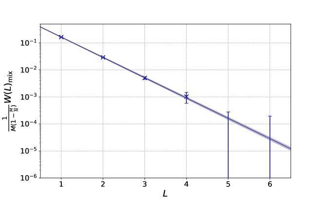
Refer to caption
Refer to caption
Figure 9: Mixed subsector Wilson loop, Wmixsubscript𝑊mixW_{\rm mix}, at T=0.29𝑇0.29T=0.29, for P=0.2𝑃0.2P=0.2 and P=0.25𝑃0.25P=0.25, respectively. We have extrapolated to the large N𝑁N limit using N=24,32,64𝑁243264N=24,32,64, and to the continuum limit using nt=16,24,32subscript𝑛𝑡162432n_{t}=16,24,32 for each N𝑁N, using the 2D interpolation 1M(1MN)Wmix(L)=γ(L)+β1N2+β2nt+β2ntN21𝑀1𝑀𝑁subscript𝑊mix𝐿𝛾𝐿subscript𝛽1superscript𝑁2subscript𝛽2subscript𝑛𝑡subscript𝛽2subscript𝑛𝑡superscript𝑁2\frac{1}{M(1-\frac{M}{N})}W_{\rm mix}(L)=\gamma(L)+\frac{\beta_{1}}{N^{2}}+\frac{\beta_{2}}{n_{t}}+\frac{\beta_{2}}{n_{t}N^{2}}. We fitted the interpolated values γ(L)𝛾𝐿\gamma(L) for 1L41𝐿41\leq L\leq 4 to the ansatz γ(L)=exp(cL+d)𝛾𝐿𝑐𝐿𝑑\gamma(L)=\exp(-cL+d). We find cmix=1.731(21)subscript𝑐mix1.73121c_{\rm mix}=1.731(21) and cmix=1.708(20)subscript𝑐mix1.70820c_{\rm mix}=1.708(20) for P=0.2𝑃0.2P=0.2 and P=0.25𝑃0.25P=0.25, respectively. The fit is shown along with error bounds by the blue line.
Refer to caption
Refer to caption
Figure 10: Combined mixed and confined subsector Wilson loop, Wcon+Wmixsubscript𝑊consubscript𝑊mixW_{\rm con}+W_{\rm mix}, at T=0.29𝑇0.29T=0.29, for P=0.2𝑃0.2P=0.2 and P=0.25𝑃0.25P=0.25, respectively. We have extrapolated to the large N𝑁N limit using N=24,32,64𝑁243264N=24,32,64, and to the continuum limit using nt=16,24,32subscript𝑛𝑡162432n_{t}=16,24,32 for each N𝑁N, using the 2D interpolation 1MN(Wcon+Wmix)(L)=γ(L)+β1N2+β2nt+β2ntN21𝑀𝑁subscript𝑊consubscript𝑊mix𝐿𝛾𝐿subscript𝛽1superscript𝑁2subscript𝛽2subscript𝑛𝑡subscript𝛽2subscript𝑛𝑡superscript𝑁2\frac{1}{M-N}(W_{\rm con}+W_{\rm mix})(L)=\gamma(L)+\frac{\beta_{1}}{N^{2}}+\frac{\beta_{2}}{n_{t}}+\frac{\beta_{2}}{n_{t}N^{2}}. We fitted these interpolated values γ(L)𝛾𝐿\gamma(L) for 1L41𝐿41\leq L\leq 4 to the ansatz γ(L)=exp(cL+d)𝛾𝐿𝑐𝐿𝑑\gamma(L)=\exp(-cL+d). We obtained c=1.733(19)𝑐1.73319c=1.733(19) and d=0.021(22)𝑑0.02122d=0.021(22) for P=0.20𝑃0.20P=0.20, and c=1.718(18)𝑐1.71818c=1.718(18) and d=0.006(21)𝑑0.00621d=-0.006(21) for P=0.25𝑃0.25P=0.25. The fit is shown along with error bounds by the blue line. The theoretical prediction is shown by the red and is mostly obscured by the fit.
Refer to caption
Refer to caption
Figure 11: Deconfined subsector Wilson loop, Wdecsubscript𝑊decW_{\rm dec}, at T=0.29𝑇0.29T=0.29, for P=0.2𝑃0.2P=0.2 and P=0.25𝑃0.25P=0.25, respectively. We used the same scale as in Figs. 8, 9, and 10. The potential is clearly nonconfining, and no fitting was attempted

Comments on temperature dependence

In the model under consideration, the partially-deconfined saddle is the maximum of the free energy. The distribution of Polyakov line phases at the saddle changes with temperature. Therefore, strictly speaking, we need to study multiple values of T𝑇T, choosing the value of P𝑃P exactly on top of the saddle. However, we explicitly confirmed that the expected behaviors (81), (82), and (87) at T=0.29𝑇0.29T=0.29 at P=0𝑃0P=0, 0.200.200.20 and 0.250.250.25, which suggests that this relation holds near the critical point regardless of the value of P𝑃P, and hence also on the partially-deconfined saddle. It is straightforward to perform the more complete analyses if more computational resources are available. We will leave it for future work. See also comments at the end of Sec. 4.

6 Conclusions and discussions

In this paper, we presented evidence for the formation of a flux tube and linear confinement potential in the confined sector of the partially-deconfined saddle of pure Yang-Mills theory by taking strongly-coupled lattice gauge theory as a concrete example. The linear confinement potential in the confined sector supports the argument given in Ref. Hanada:2019kue concerning the ’t Hooft anomaly matching associated with the chiral symmetry breaking in the confined sector. Namely, quarks in the confined sector must form a bound state, and then the pion should be formed in the confined sector so that the anomaly-matching condition is satisfied. It can also explain the observation in Ref. Hanada:2021ksu , i.e., chiral symmetry breaks spontaneously at the complete deconfinement/partial deconfinement phase transition point, because the formation of chiral condensate in the confined sector is sufficient to break the chiral symmetry.

By studying large-N𝑁N QCD in the Veneziano limit with sufficiently light quarks, we should be able to see the stable partially-deconfined phase. It would be interesting to see whether chiral symmetry breaking and the complete deconfinement/partial deconfinement phase transition coincide. Another interesting direction would be to explore whether partial confinement is a sharp notion for SU(3) real-world QCD (see Ref. Hanada:2021ksu ).

Our result means that, in the partially-deconfined phase, the probe quark-antiquark potential behaves differently in the confined and deconfined sectors. In the holographic calculation of the Wilson loop Maldacena:1998im , this would mean that different worldsheets are preferred in the confined and deconfined sectors. We have not understood how it affects the conventional computations on the gravity side.

The original motivation Hanada:2016pwv for considering partial deconfinement was to understand the emergent geometry in gauge/gravity duality. Naturally, the deconfined sector is interpreted as a black hole. The findings in this paper are consistent with the expectation that short strings, which correspond to gravitons when there is a gravity dual, can live in the confined sector Hanada:2021ipb ; Hanada:2021swb ; Gautam:2022akq . When applied to the evaporating black hole, the Page curve Page:1993wv follows from this interpretation Gautam:2022akq . It would be interesting if we can deepen our understanding of the roles matrix degrees of freedom play in the emergent geometry.

Acknowledgement

We thank Georg Bergner, Thomas Cohen, Robert Pisarski, and Hiromasa Watanabe for useful discussions and comments. V.G. thanks STFC for Doctoral Training Programme funding (ST/W507854-2021 Maths DTP). M.H. thanks the STFC Ernest Rutherford Grant ST/R003599/1. J.H. thanks STFC for the support of a studentship. E.R. is supported by Nippon Telegraph and Telephone Corporation (NTT) Research.

Data management

No additional research data beyond the data presented and cited in this work are needed to validate the research findings in this work. Simulation data will be publicly available after publication on Zenodo.

Appendix A Constrained simulations of the first kind and second kind
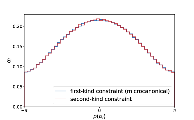
Refer to caption
Figure 12: Polyakov loop phase distributions for N=64𝑁64N=64, nt=32subscript𝑛𝑡32n_{t}=32, P=0.2𝑃0.2P=0.2, for constraints of the first and second kind.

A potential objection to our approach might be the apparent unnaturalness of the constraint simulation of the second kind. Here, we justify the second constraint as being equivalent to fixing some of the gauge redundancy that remains after having taken static diagonal gauge. The second constraint imposes uniformity on some subset NM𝑁𝑀N-M of the eigenvalues of the Polyakov loop. In a general configuration at finite N𝑁N outputted by the Monte-Carlo simulation under the constraint of the first kind, a subset of eigenvalues is not guaranteed to be exactly uniformly distributed in this way. However, at large N𝑁N, the constraint of the second-kind and fixing of residual gauge symmetry should be equivalent, with fluctuations away from the mean value being suppressed. If the Polyakov eigenvalue distributions are identical between the microcanonical (first-kind constrained) and second-constrained simulation, we can use our method as an effective gauge fixing in the large-N𝑁N limit. As we can see from Fig. 12, constrained simulations with the 1st and 2nd constraints indeed give the same distribution of the Polyakov-loop phases. Furthermore, as we can see Fig. 13, the distributions of α1,,αMsubscript𝛼1subscript𝛼𝑀\alpha_{1},\cdots,\alpha_{M} and αM+1,,αNsubscript𝛼𝑀1subscript𝛼𝑁\alpha_{M+1},\cdots,\alpha_{N} exhibit the kind splitting depicted in Fig. 3.
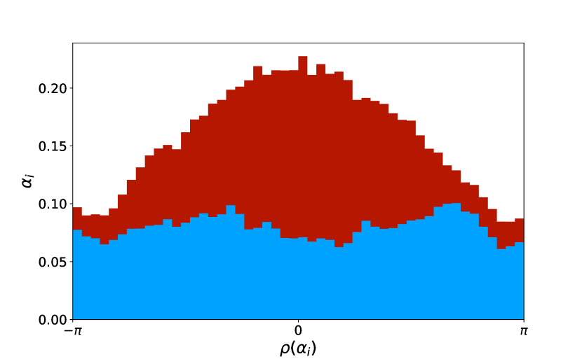
Refer to caption
(a)
Refer to caption
(b)
Refer to caption
(c)
Refer to caption
(d)
Refer to caption
(e)
Refer to caption
(f)
Figure 13: Polyakov loop phase distributions for N=32𝑁32N=32 and N=64𝑁64N=64, nt=24subscript𝑛𝑡24n_{t}=24, P=0.2𝑃0.2P=0.2 (top) and P=0.25𝑃0.25P=0.25 (bottom), for constraints of the second kind. In addition to the distribution of all phases, the ‘deconfined part’ (α1,,αMsubscript𝛼1subscript𝛼𝑀\alpha_{1},\cdots,\alpha_{M}) and ‘confined part’ (αM+1,,αNsubscript𝛼𝑀1subscript𝛼𝑁\alpha_{M+1},\cdots,\alpha_{N}) are shown.

We can also check that the confined Polyakov loop correlator exhibits an area law in the microcanonical ensemble, without the imposition of uniformity on the confined subsector that is done in the constrained simulations of the second kind. We reasoned that the Wilson loop obtained in the constrained simulation of the first kind must be the sum of the contributions from Wconsubscript𝑊conW_{\rm con}, Wdecsubscript𝑊decW_{\rm dec} and Wmixsubscript𝑊mixW_{\rm mix}, and that the constrained simulation of second kind separates these pieces neatly. One may wonder whether this method of explicit separation does something more and spoils the partially-deconfined saddle. As a consistency check, we can subtract the deconfined-sector Wilson loop computed from the second-kind simulations from the first-kind Wilson loop to obtain a quantity with an area law, as expected from the confined and mixed sectors. More advantageously, we can calculate,

Wsubtracted=Wfull,1stWdec,2ndWmix,2nd.subscript𝑊subtractedsubscript𝑊full1stsubscript𝑊dec2ndsubscript𝑊mix2nd\displaystyle W_{\rm subtracted}=W_{\rm full,1st}-W_{\rm dec,2nd}-W_{\rm mix,2nd}. (88)

This Wsubtractedsubscript𝑊subtractedW_{\rm subtracted} should be the sum of Wconsubscript𝑊conW_{\rm con} and Wmixsubscript𝑊mixW_{\rm mix}, and hence, Wsubtracted=(NM)exp(σLβ)subscript𝑊subtracted𝑁𝑀𝜎𝐿𝛽W_{\rm subtracted}=(N-M)\exp(-\sigma L\beta) is expected.

This demonstrates that the linear potential is not the result of an artifical imposition of uniformity on the eigenvalues, but is present even in the constrained simulations of the first kind. We also find by this analysis that the constraint of the second kind approximates the gauge-fixed microcanonical ensemble well even at N=16𝑁16N=16.

Refer to caption
Figure 14: The complete Wilson loop from first-kind simulations, the deconfined Wilson loop from second-kind simulations, and their difference, nt=32subscript𝑛𝑡32n_{t}=32 and T=0.29𝑇0.29T=0.29, extrapolated to large N𝑁N. Note that the continuum limit has not been taken.

In Fig. 14, we plotted Wsubtractedsubscript𝑊subtractedW_{\rm subtracted}. As expected, by subtracting the contribution from the deconfined sector, we find confining behaviour matching that of the mixed and confined subgroups from second-kind simulations.

Appendix B Stability of the extrapolations

Small N𝑁N effects

We collected data for N=16,24,32,64𝑁16243264N=16,24,32,64. For the large-N𝑁N extrapolation of Wconsubscript𝑊conW_{\rm con} (respectively, Wmixsubscript𝑊mixW_{\rm mix}), we should use only the data points with sufficiently large NM𝑁𝑀N-M (respectively, M𝑀M and NM𝑁𝑀N-M). However, for P=0.25𝑃0.25P=0.25, the N=16𝑁16N=16 data seemed to present a source of systematic error from finite N𝑁N, M𝑀M, and NM𝑁𝑀N-M effects. In particular, for N=16𝑁16N=16 and P=0.25𝑃0.25P=0.25 we have NM=6𝑁𝑀6N-M=6. Such errors would not be captured by the error bars. We can measure the contribution to the systematic error by removing data at different values of N𝑁N from the interpolation. The effect of this on the fitting parameter c𝑐c is shown in Tables BB, and B.

It is easy to understand how the N=16𝑁16N=16 data is distorting the results when we attempt a linear fit. We demonstrate this in Fig. 15. The small value of NM𝑁𝑀N-M causes the N=16𝑁16N=16 point to be far separated from the others on the x axis. Consequently, it has a large effect on the linear fit. There is also clear non-linear behaviour. For P=0.2𝑃0.2P=0.2, NM𝑁𝑀N-M is larger, and this explains why the distortion is not so severe. We could have attempted a quadratic fit, but we see from Fig. 15 that this does not significantly reduce the uncertainty, and potentially increases it. Therefore, we performed the large-N𝑁N extrapolations in the main text without using N=16𝑁16N=16.

Small ntsubscript𝑛𝑡n_{t} effects

We see a similar issue with respect to nt=16subscript𝑛𝑡16n_{t}=16. In Table B and Table B, we see that c𝑐c for P=0.25𝑃0.25P=0.25 is smaller than the theoretical value 1.7241.7241.724, whether N=16𝑁16N=16 is removed or not. We attribute this to the use of nt=16subscript𝑛𝑡16n_{t}=16. If we plot points at nt=16,24subscript𝑛𝑡1624n_{t}=16,24 and 323232 with fixed N𝑁N and L𝐿L by taking 1nt1subscript𝑛𝑡\frac{1}{n_{t}} as the horizontal axis, we can see that those three points are not always on a straight line and a linear fit is often very bad. This happens for both P=0.2𝑃0.2P=0.2 and P=0.25𝑃0.25P=0.25. For the analyses in the main text, we did not include nt=16subscript𝑛𝑡16n_{t}=16 for either P=0.2𝑃0.2P=0.2 or P=0.25𝑃0.25P=0.25. The effect of removing nt=16subscript𝑛𝑡16n_{t}=16 can be seen by comparing Tables BBB with Tables BBB.

P𝑃P all N𝑁N rmv. N=16𝑁16N=16 rmv. N=24𝑁24N=24 rmv. N=32𝑁32N=32 rmv. N=64𝑁64N=64
\csvreader[head to column names, late after line=
\csvcolvi \csvcolii \csvcoliii \csvcoliv \csvcolv
Table 3: Values of c𝑐c for Wcon+Wmixsubscript𝑊consubscript𝑊mixW_{\rm con}+W_{\rm mix} with data for different N𝑁N removed. With nt=16subscript𝑛𝑡16n_{t}=16.
P𝑃P all N𝑁N rmv. N=16𝑁16N=16 rmv. N=24𝑁24N=24 rmv. N=32𝑁32N=32 rmv. N=64𝑁64N=64
\csvreader[head to column names, late after line=
\csvcolvi \csvcolii \csvcoliii \csvcoliv \csvcolv
Table 4: Values of cconsubscript𝑐conc_{\rm con} for Wconsubscript𝑊conW_{\rm con} with data for different N𝑁N removed. With nt=16subscript𝑛𝑡16n_{t}=16.
P𝑃P all N𝑁N rmv. N=16𝑁16N=16 rmv. N=24𝑁24N=24 rmv. N=32𝑁32N=32 rmv. N=64𝑁64N=64
\csvreader[head to column names, late after line=
\csvcolvi \csvcolii \csvcoliii \csvcoliv \csvcolv
Table 5: Values of cmixsubscript𝑐mixc_{\rm mix} for Wmixsubscript𝑊mixW_{\rm mix} with data for different N𝑁N removed. With nt=16subscript𝑛𝑡16n_{t}=16.
P𝑃P all N𝑁N rmv. N=16𝑁16N=16 rmv. N=24𝑁24N=24 rmv. N=32𝑁32N=32 rmv. N=64𝑁64N=64
\csvreader[head to column names, late after line=
\csvcolvi \csvcolii \csvcoliii \csvcoliv \csvcolv
Table 6: Values of c𝑐c for Wcon+Wmixsubscript𝑊consubscript𝑊mixW_{\rm con}+W_{\rm mix} with data for different N𝑁N removed. Without nt=16subscript𝑛𝑡16n_{t}=16.
P𝑃P all N𝑁N rmv. N=16𝑁16N=16 rmv. N=24𝑁24N=24 rmv. N=32𝑁32N=32 rmv. N=64𝑁64N=64
\csvreader[head to column names, late after line=
\csvcolvi \csvcolii \csvcoliii \csvcoliv \csvcolv
Table 7: Values of cconsubscript𝑐conc_{\rm con} for Wconsubscript𝑊conW_{\rm con} with data for different N𝑁N removed. Without nt=16subscript𝑛𝑡16n_{t}=16.
P𝑃P all N𝑁N rmv. N=16𝑁16N=16 rmv. N=24𝑁24N=24 rmv. N=32𝑁32N=32 rmv. N=64𝑁64N=64
\csvreader[head to column names, late after line=
\csvcolvi \csvcolii \csvcoliii \csvcoliv \csvcolv
Table 8: Values of cmixsubscript𝑐mixc_{\rm mix} for Wmixsubscript𝑊mixW_{\rm mix} with data for different N𝑁N removed. Without nt=16subscript𝑛𝑡16n_{t}=16.
Refer to caption
Refer to caption
Figure 15: Performing the large N𝑁N extrapolation for the confined subsector P=0.2𝑃0.2P=0.2 (left) and P=0.25𝑃0.25P=0.25 (right) for L=1𝐿1L=1. The continuum limit ntsubscript𝑛𝑡n_{t}\rightarrow\infty has been taken. We try a linear fit of all points (green), a linear fit that ignores N=16𝑁16N=16 (red), and a quadratic fit of all points (orange). The destabilising effect of the N=16𝑁16N=16 (rightmost) point in the P=0.25𝑃0.25P=0.25 linear extrapolation is obvious and can be attributed to the small value NM=6𝑁𝑀6N-M=6.

Appendix C Gauge fixing condition and separation of confined and deconfined sectors

As a starter, let us recall how the operator formalism and path-integral formalism are related (see e.g., Rinaldi:2021jbg for the case of Hermitian variables). The thermal partition function of the Eguchi-Kawai model is

Z(T)𝑍𝑇\displaystyle Z(T) =1[volU(N)]K(k=1Kdgk)Trext(g^(K)eH(E^,U^)TKg^(K1)1g^(K1)\displaystyle=\frac{1}{[{\rm volU}(N)]^{K}}\int\left(\prod_{k=1}^{K}dg_{k}\right){\rm Tr}_{{\cal H}_{\rm ext}}\Bigl{(}\hat{g}_{(K)}e^{-\frac{H(\hat{E},\hat{U})}{TK}}\hat{g}_{(K-1)}^{-1}\hat{g}_{(K-1)}
eH(E^,U^)TKg^(K2)1g^(K2)g^(1)1g^(1)eH(E^,U^)TK)\displaystyle\quad e^{-\frac{H(\hat{E},\hat{U})}{TK}}\hat{g}_{(K-2)}^{-1}\hat{g}_{(K-2)}\cdots\hat{g}_{(1)}^{-1}\hat{g}_{(1)}e^{-\frac{H(\hat{E},\hat{U})}{TK}}\Bigl{)}
=1[volU(N)]K(k=1Kdg(k))(k=1KdU(k))absent1superscriptdelimited-[]volU𝑁𝐾superscriptsubscriptproduct𝑘1𝐾𝑑subscript𝑔𝑘superscriptsubscriptproduct𝑘1𝐾𝑑subscript𝑈𝑘\displaystyle=\frac{1}{[{\rm volU}(N)]^{K}}\int\left(\prod_{k=1}^{K}dg_{(k)}\right)\int\left(\prod_{k=1}^{K}dU_{(k)}\right)
U(K)|g^(K)eH(E^,U^)TKg^(K1)1|U(K1)quantum-operator-productsubscript𝑈𝐾subscript^𝑔𝐾superscript𝑒𝐻^𝐸^𝑈𝑇𝐾superscriptsubscript^𝑔𝐾11subscript𝑈𝐾1\displaystyle\qquad\langle U_{(K)}|\hat{g}_{(K)}e^{-\frac{H(\hat{E},\hat{U})}{TK}}\hat{g}_{(K-1)}^{-1}|U_{(K-1)}\rangle
×U(K1)|g^(K1)eH(E^,U^)TKg^(K2)1|U(K2)absentquantum-operator-productsubscript𝑈𝐾1subscript^𝑔𝐾1superscript𝑒𝐻^𝐸^𝑈𝑇𝐾superscriptsubscript^𝑔𝐾21subscript𝑈𝐾2\displaystyle\qquad\times\langle U_{(K-1)}|\hat{g}_{(K-1)}e^{-\frac{H(\hat{E},\hat{U})}{TK}}\hat{g}_{(K-2)}^{-1}|U_{(K-2)}\rangle
××U(1)|g^(1)eH(E^,U^)TK|U(K).absentquantum-operator-productsubscript𝑈1subscript^𝑔1superscript𝑒𝐻^𝐸^𝑈𝑇𝐾subscript𝑈𝐾\displaystyle\qquad\times\cdots\times\langle U_{(1)}|\hat{g}_{(1)}e^{-\frac{H(\hat{E},\hat{U})}{TK}}|U_{(K)}\rangle. (89)

For H(E^,U^)=12TrE^2+V(U^)𝐻^𝐸^𝑈12Trsuperscript^𝐸2𝑉^𝑈H(\hat{E},\hat{U})=\frac{1}{2}{\rm Tr}\hat{E}^{2}+V(\hat{U}), we can rewrite each term in the product as follows.

U(k)|g^(k)eH(E^,U^)TKg^(k1)1|U(k1)quantum-operator-productsubscript𝑈𝑘subscript^𝑔𝑘superscript𝑒𝐻^𝐸^𝑈𝑇𝐾superscriptsubscript^𝑔𝑘11subscript𝑈𝑘1\displaystyle\langle U_{(k)}|\hat{g}_{(k)}e^{-\frac{H(\hat{E},\hat{U})}{TK}}\hat{g}_{(k-1)}^{-1}|U_{(k-1)}\rangle
=g(k)1U(k)g(k)|eH(E^,U^)TK|g(k1)1U(k1)g(k1)absentquantum-operator-productsubscriptsuperscript𝑔1𝑘subscript𝑈𝑘subscript𝑔𝑘superscript𝑒𝐻^𝐸^𝑈𝑇𝐾subscriptsuperscript𝑔1𝑘1subscript𝑈𝑘1subscript𝑔𝑘1\displaystyle\quad=\langle g^{-1}_{(k)}U_{(k)}g_{(k)}|e^{-\frac{H(\hat{E},\hat{U})}{TK}}|g^{-1}_{(k-1)}U_{(k-1)}g_{(k-1)}\rangle
=e1TKV(g(k1)1U(k1)g(k1))g(k)1U(k)g(k)|e12TKTrE^2|g(k1)1U(k1)g(k1).absentsuperscript𝑒1𝑇𝐾𝑉subscriptsuperscript𝑔1𝑘1subscript𝑈𝑘1subscript𝑔𝑘1quantum-operator-productsubscriptsuperscript𝑔1𝑘subscript𝑈𝑘subscript𝑔𝑘superscript𝑒12𝑇𝐾Trsuperscript^𝐸2subscriptsuperscript𝑔1𝑘1subscript𝑈𝑘1subscript𝑔𝑘1\displaystyle\quad=e^{-\frac{1}{TK}V(g^{-1}_{(k-1)}U_{(k-1)}g_{(k-1)})}\langle g^{-1}_{(k)}U_{(k)}g_{(k)}|e^{-\frac{1}{2TK}{\rm Tr}\hat{E}^{2}}|g^{-1}_{(k-1)}U_{(k-1)}g_{(k-1)}\rangle. (90)

By using

iϵlog(g(k)1U(k)g(k)g(k1)1U(k1)1g(k1)),𝑖italic-ϵsuperscriptsubscript𝑔𝑘1subscript𝑈𝑘subscript𝑔𝑘superscriptsubscript𝑔𝑘11subscriptsuperscript𝑈1𝑘1subscript𝑔𝑘1\displaystyle i\epsilon\equiv\log\left(g_{(k)}^{-1}U_{(k)}g_{(k)}g_{(k-1)}^{-1}U^{-1}_{(k-1)}g_{(k-1)}\right), (91)

we can relate |g(k1)1U(k1)g(k1)ketsubscriptsuperscript𝑔1𝑘1subscript𝑈𝑘1subscript𝑔𝑘1|g^{-1}_{(k-1)}U_{(k-1)}g_{(k-1)}\rangle and |g(k)1U(k)g(k)ketsubscriptsuperscript𝑔1𝑘subscript𝑈𝑘subscript𝑔𝑘|g^{-1}_{(k)}U_{(k)}g_{(k)}\rangle as

|g(k)1U(k)g(k)=eiTr(ϵE^)|g(k1)1U(k1)g(k1),ketsubscriptsuperscript𝑔1𝑘subscript𝑈𝑘subscript𝑔𝑘superscript𝑒𝑖Tritalic-ϵ^𝐸ketsubscriptsuperscript𝑔1𝑘1subscript𝑈𝑘1subscript𝑔𝑘1\displaystyle|g^{-1}_{(k)}U_{(k)}g_{(k)}\rangle=e^{i{\rm Tr}(\epsilon\hat{E})}|g^{-1}_{(k-1)}U_{(k-1)}g_{(k-1)}\rangle, (92)

and hence,

g(k)1U(k)g(k)|e12TKTrE^2|g(k1)1U(k1)g(k1)quantum-operator-productsubscriptsuperscript𝑔1𝑘subscript𝑈𝑘subscript𝑔𝑘superscript𝑒12𝑇𝐾Trsuperscript^𝐸2subscriptsuperscript𝑔1𝑘1subscript𝑈𝑘1subscript𝑔𝑘1\displaystyle\langle g^{-1}_{(k)}U_{(k)}g_{(k)}|e^{-\frac{1}{2TK}{\rm Tr}\hat{E}^{2}}|g^{-1}_{(k-1)}U_{(k-1)}g_{(k-1)}\rangle
=g(k1)1U(k1)g(k1)|e12TKTrE^2iTr(ϵE^)|g(k1)1U(k1)g(k1)absentquantum-operator-productsubscriptsuperscript𝑔1𝑘1subscript𝑈𝑘1subscript𝑔𝑘1superscript𝑒12𝑇𝐾Trsuperscript^𝐸2𝑖Tritalic-ϵ^𝐸subscriptsuperscript𝑔1𝑘1subscript𝑈𝑘1subscript𝑔𝑘1\displaystyle=\langle g^{-1}_{(k-1)}U_{(k-1)}g_{(k-1)}|e^{-\frac{1}{2TK}{\rm Tr}\hat{E}^{2}-i{\rm Tr}(\epsilon\hat{E})}|g^{-1}_{(k-1)}U_{(k-1)}g_{(k-1)}\rangle
=U|e12TKTrE^2iTr(ϵE^)|U,absentquantum-operator-product𝑈superscript𝑒12𝑇𝐾Trsuperscript^𝐸2𝑖Tritalic-ϵ^𝐸𝑈\displaystyle=\langle U|e^{-\frac{1}{2TK}{\rm Tr}\hat{E}^{2}-i{\rm Tr}(\epsilon\hat{E})}|U\rangle, (93)

where U𝑈U can be any element of the unitary group.777 Because TrE^2Trsuperscript^𝐸2{\rm Tr}\hat{E}^{2} commutes with the shift on the group manifold, the first line could be Wg(k)1U(k)g(k)|e12TKTrE^2|Wg(k1)1U(k1)g(k1)quantum-operator-product𝑊subscriptsuperscript𝑔1𝑘subscript𝑈𝑘subscript𝑔𝑘superscript𝑒12𝑇𝐾Trsuperscript^𝐸2𝑊subscriptsuperscript𝑔1𝑘1subscript𝑈𝑘1subscript𝑔𝑘1\langle Wg^{-1}_{(k)}U_{(k)}g_{(k)}|e^{-\frac{1}{2TK}{\rm Tr}\hat{E}^{2}}|Wg^{-1}_{(k-1)}U_{(k-1)}g_{(k-1)}\rangle, where W𝑊W is an arbitrary element of U(N𝑁N). Up to a normalization constant, this can be written by using trace over the Hilbert space as

Trexp(12KTαE^α2+iαϵαE^α)Tr12𝐾𝑇subscript𝛼superscriptsubscript^𝐸𝛼2𝑖subscript𝛼superscriptitalic-ϵ𝛼subscript^𝐸𝛼\displaystyle\textrm{Tr}\exp\left(-\frac{1}{2KT}\sum_{\alpha}\hat{E}_{\alpha}^{2}+i\sum_{\alpha}\epsilon^{\alpha}\hat{E}_{\alpha}\right)
=eKT2Trϵ2×Trexp(12KTα(E^αiKTϵα)2).absentsuperscript𝑒𝐾𝑇2Trsuperscriptitalic-ϵ2Tr12𝐾𝑇subscript𝛼superscriptsubscript^𝐸𝛼𝑖𝐾𝑇subscriptitalic-ϵ𝛼2\displaystyle=e^{-\frac{KT}{2}{\rm Tr}\epsilon^{2}}\times{\rm Tr}\exp\left(-\frac{1}{2KT}\sum_{\alpha}(\hat{E}_{\alpha}-iKT\epsilon_{\alpha})^{2}\right). (94)

The second term (TrTr{\rm Tr}\cdots) becomes constant in the limit of KT𝐾𝑇KT\to\infty when KTϵ2𝐾𝑇superscriptitalic-ϵ2KT\epsilon^{2} is of order one (which is justified because of the first term eKT2Trϵ2superscript𝑒𝐾𝑇2Trsuperscriptitalic-ϵ2e^{-\frac{KT}{2}{\rm Tr}\epsilon^{2}}), because the sum over momentum modes can be identified with usual integral in flat space. Omitting the second term and by approximating ϵ2superscriptitalic-ϵ2\epsilon^{2} by |g(k)1U(k)g(k)g(k1)1U(k1)g(k1)|2superscriptsuperscriptsubscript𝑔𝑘1subscript𝑈𝑘subscript𝑔𝑘superscriptsubscript𝑔𝑘11subscript𝑈𝑘1subscript𝑔𝑘12|g_{(k)}^{-1}U_{(k)}g_{(k)}-g_{(k-1)}^{-1}U_{(k-1)}g_{(k-1)}|^{2}, we obtain

eKT2Tr[|g(k)1U(k)g(k)g(k1)1U(k1)g(k1)|2]eV(g(k)1U(k)g(k))/(TK)superscript𝑒𝐾𝑇2Trdelimited-[]superscriptsuperscriptsubscript𝑔𝑘1subscript𝑈𝑘subscript𝑔𝑘superscriptsubscript𝑔𝑘11subscript𝑈𝑘1subscript𝑔𝑘12superscript𝑒𝑉superscriptsubscript𝑔𝑘1subscript𝑈𝑘subscript𝑔𝑘𝑇𝐾\displaystyle e^{-\frac{KT}{2}{\rm Tr}[|g_{(k)}^{-1}U_{(k)}g_{(k)}-g_{(k-1)}^{-1}U_{(k-1)}g_{(k-1)}|^{2}]}e^{-V(g_{(k)}^{-1}U_{(k)}g_{(k)})/(TK)}
eL[Dt(g(k)1U(k)g(k)),(g(k)1U(k)g(k))]/(TK)similar-to-or-equalsabsentsuperscript𝑒𝐿subscript𝐷𝑡superscriptsubscript𝑔𝑘1subscript𝑈𝑘subscript𝑔𝑘superscriptsubscript𝑔𝑘1subscript𝑈𝑘subscript𝑔𝑘𝑇𝐾\displaystyle\quad\simeq e^{-L[D_{t}(g_{(k)}^{-1}U_{(k)}g_{(k)}),(g_{(k)}^{-1}U_{(k)}g_{(k)})]/(TK)}
=eL[DtU(k),U(k))]/(TK).\displaystyle\quad=e^{-L[D_{t}U_{(k)},U_{(k)})]/(TK)}. (95)

Here we used

g(k1)g(k)1eiA(k)/(KT),subscript𝑔𝑘1superscriptsubscript𝑔𝑘1superscript𝑒𝑖subscript𝐴𝑘𝐾𝑇\displaystyle g_{(k-1)}g_{(k)}^{-1}\equiv e^{-iA_{(k)}/(KT)}, (96)

and

U(k)(g(k1)g(k)1)1U(k1)(g(k1)g(k)1)DtU(k)KT.similar-to-or-equalssubscript𝑈𝑘superscriptsubscript𝑔𝑘1superscriptsubscript𝑔𝑘11subscript𝑈𝑘1subscript𝑔𝑘1superscriptsubscript𝑔𝑘1subscript𝐷𝑡subscript𝑈𝑘𝐾𝑇\displaystyle U_{(k)}-(g_{(k-1)}g_{(k)}^{-1})^{-1}U_{(k-1)}(g_{(k-1)}g_{(k)}^{-1})\simeq\frac{D_{t}U_{(k)}}{KT}. (97)

By taking K𝐾K\to\infty limit, we obtain

Z(T)𝑍𝑇\displaystyle Z(T) =[dA][dU]e𝑑tL[DtU,U].absentdelimited-[]𝑑𝐴delimited-[]𝑑𝑈superscript𝑒differential-d𝑡𝐿subscript𝐷𝑡𝑈𝑈\displaystyle=\int[dA][dU]e^{-\int dtL[D_{t}U,U]}. (98)

Note that g(K)subscript𝑔𝐾g_{(K)} is the Polyakov loop. In the static diagonal gauge,

g(k)=diag(eikθ1/K,,eikθN/K).subscript𝑔𝑘diagsuperscript𝑒𝑖𝑘subscript𝜃1𝐾superscript𝑒𝑖𝑘subscript𝜃𝑁𝐾\displaystyle g_{(k)}={\rm diag}(e^{ik\theta_{1}/K},\cdots,e^{ik\theta_{N}/K}). (99)

In the confined sector, the distribution of the phases of the Polyakov loop is uniform Hanada:2020uvt . We fix the SN permutation symmetry such that the phase distribution does indeed satisfy this property. This guarantees the neat separation into confined and deconfined sectors at t=β𝑡𝛽t=\beta (equivalently, t=0𝑡0t=0).

Let us use the trace cyclicity in the extended Hilbert space and shift the initial time. In the static diagonal gauge, this does not change the Polyakov loop. Therefore, exactly the same separation into confined and deconfined sectors holds at any t𝑡t.

Appendix D Simulation algorithm

Several aspects of the simulation algorithm used for this study are similar to the one used in Ref. Berkowitz:2016jlq , which was originally developed in unpublished work by one of the authors (MH), Takashi Kaneko, Jun Nishimura, and Asato Tsuchiya in 2013.

The lattice action we consider is, before adding the constraint term for the Polyakov loop,

S=N2aμ=1dt=1ntTr(1NUμ,tVUμ,t+1V)+h.c.+SF.P.,formulae-sequence𝑆𝑁2𝑎superscriptsubscript𝜇1𝑑superscriptsubscript𝑡1subscript𝑛𝑡Trsubscript1𝑁subscript𝑈𝜇𝑡𝑉superscriptsubscript𝑈𝜇𝑡1superscript𝑉hcsubscript𝑆formulae-sequence𝐹𝑃\displaystyle S=\frac{N}{2a}\sum_{\mu=1}^{d}\sum_{t=1}^{n_{t}}{\rm Tr}\left(\textbf{1}_{N}-U_{\mu,t}VU_{\mu,t+1}^{\dagger}V^{\dagger}\right)+{\rm h.c.}+S_{F.P.}, (100)

where V=diag(eiα1/nt,,eiαN/nt)𝑉diagsuperscript𝑒𝑖subscript𝛼1subscript𝑛𝑡superscript𝑒𝑖subscript𝛼𝑁subscript𝑛𝑡V={\rm diag}(e^{i\alpha_{1}/n_{t}},\cdots,e^{i\alpha_{N}/n_{t}}). Here, a𝑎a is the lattice spacing and β=ant𝛽𝑎subscript𝑛𝑡\beta=an_{t} is the inverse temperature, β=T1𝛽superscript𝑇1\beta=T^{-1}. We will focus on d=3𝑑3d=3. The Polyakov line phases α1,2,,Nsubscript𝛼12𝑁\alpha_{1,2,\cdots,N} are constrained to be

π<αiπ.𝜋subscript𝛼𝑖𝜋\displaystyle-\pi<\alpha_{i}\leq\pi. (101)

The Faddeev-Popov term SF.P.subscript𝑆formulae-sequence𝐹𝑃S_{F.P.} is given by

SF.P.=i<j2log|sin(αiαj2)|.subscript𝑆formulae-sequence𝐹𝑃subscript𝑖𝑗2subscript𝛼𝑖subscript𝛼𝑗2\displaystyle S_{F.P.}=-\sum_{i<j}2\log\left|\sin\left(\frac{\alpha_{i}-\alpha_{j}}{2}\right)\right|. (102)

If we just impose the constraint π<αiπ𝜋subscript𝛼𝑖𝜋-\pi<\alpha_{i}\leq\pi as it is, then the simulation is not very efficient – the ‘center of mass’ (iαi)/Nsubscript𝑖subscript𝛼𝑖𝑁(\sum_{i}\alpha_{i})/N randomly moves and hits ±πplus-or-minus𝜋\pm\pi. For this reason, we use the following trick.

Firstly, let us recall that αisubscript𝛼𝑖\alpha_{i} and α~iαiCsubscript~𝛼𝑖subscript𝛼𝑖𝐶\tilde{\alpha}_{i}\equiv\alpha_{i}-C give the same weight for any C𝐶C. Here, C𝐶C must satisfy min(α~i)+C>πminsubscript~𝛼𝑖𝐶𝜋{\rm min}(\tilde{\alpha}_{i})+C>-\pi and max(α~i)+Cπmaxsubscript~𝛼𝑖𝐶𝜋{\rm max}(\tilde{\alpha}_{i})+C\leq\pi, because of the condition π<αiπ𝜋subscript𝛼𝑖𝜋-\pi<\alpha_{i}\leq\pi. Hence C𝐶C must sit in (πmin(α~i),πmax(α~i)]𝜋minsubscript~𝛼𝑖𝜋maxsubscript~𝛼𝑖(-\pi-{\rm min}(\tilde{\alpha}_{i}),\pi-{\rm max}(\tilde{\alpha}_{i})], whose interval is 2πμ2𝜋𝜇2\pi-\mu, where μmax(α~i)min(α~i)𝜇maxsubscript~𝛼𝑖minsubscript~𝛼𝑖\mu\equiv{\rm max}(\tilde{\alpha}_{i})-{\rm min}(\tilde{\alpha}_{i}). Therefore, we can replace the integral over αisubscript𝛼𝑖\alpha_{i} with that over α~isubscript~𝛼𝑖\tilde{\alpha}_{i}, with an additional Boltzmann weight

w(μ)={2πμ(μ<2π)0(μ2π).𝑤𝜇cases2𝜋𝜇𝜇2𝜋0𝜇2𝜋\displaystyle w(\mu)=\left\{\begin{array}[]{cc}2\pi-\mu&(\mu<2\pi)\\ 0&(\mu\geq 2\pi).\end{array}\right. (105)

For numerical calculations, this is not very nice because of the singularity at μ=2π𝜇2𝜋\mu=2\pi. Instead, in the molecular evolution, we use

w~(μ)={2πμ+ε(μ<2π)εegα(μ2π)(μ2π),~𝑤𝜇cases2𝜋𝜇𝜀𝜇2𝜋𝜀superscript𝑒subscript𝑔𝛼𝜇2𝜋𝜇2𝜋\displaystyle\tilde{w}(\mu)=\left\{\begin{array}[]{cc}2\pi-\mu+\varepsilon&(\mu<2\pi)\\ \varepsilon e^{-g_{\alpha}(\mu-2\pi)}&(\mu\geq 2\pi),\end{array}\right. (108)

with a large enough gαsubscript𝑔𝛼g_{\alpha} (say gαsubscript𝑔𝛼g_{\alpha}=100) and ε=gα1𝜀superscriptsubscript𝑔𝛼1\varepsilon=g_{\alpha}^{-1}. For the Metropolis test, we use w(μ)𝑤𝜇w(\mu) instead of w~(μ)~𝑤𝜇\tilde{w}(\mu). The detailed balance condition is not violated and the correct path-integral weight is reproduced; see e.g., Ref. Hanada-Matsuura .

Permutation of Polyakov line phases in the constrained simulation of second kind

When ΔSdecΔsubscript𝑆dec\Delta S_{\rm dec} and ΔSconΔsubscript𝑆con\Delta S_{\rm con} are added, the SN permutation symmetry is explicitly broken to S×M{}_{M}\timesSN-M. The ordering of the α𝛼\alpha’s — say αi1<αi2<αi3<subscript𝛼subscript𝑖1subscript𝛼subscript𝑖2subscript𝛼subscript𝑖3\alpha_{i_{1}}<\alpha_{i_{2}}<\alpha_{i_{3}}<\cdots — does not change (or very rarely changes) in the HMC simulation, which can cause a problem when the permutation symmetry is explicitly broken. To avoid this problem, we choose αisubscript𝛼𝑖\alpha_{i} and αjsubscript𝛼𝑗\alpha_{j} randomly from the deconfined and confined sectors and perform a permutation using the Metropolis algorithm. Note that the i𝑖i-th and j𝑗j-th rows and columns in Uμsubscript𝑈𝜇U_{\mu} have to be exchanged, too. We do this 10 times after each HMC steps. This method is the same as the one used in Ref. Watanabe:2020ufk .

N𝑁N      W𝑊W(1)      W𝑊W(2)      W𝑊W(3)      W𝑊W(4)      W𝑊W(5)
\csvreader[head to column names, late after line=
\csvcolvi \csvcolii \csvcoliii \csvcoliv \csvcolv
Table 9: Wilson loop for L=1,2,3,4,5𝐿12345L=1,2,3,4,5, unconstrained, nt=24subscript𝑛𝑡24n_{t}=24, T=0.25𝑇0.25T=0.25.
P𝑃P N𝑁N ntsubscript𝑛𝑡n_{t}     W𝑊W(1)     W𝑊W(2)     W𝑊W(3)     W𝑊W(4)     W𝑊W(5)
\csvreader[head to column names, late after line=
\csvcolviii \csvcolii \csvcoliii \csvcoliv \csvcolv \csvcolvi \csvcolvii
Table 10: Wconsubscript𝑊conW_{\rm con} for L=1,2,3,4,5𝐿12345L=1,2,3,4,5, constrained, T=0.29𝑇0.29T=0.29.
P𝑃P N𝑁N ntsubscript𝑛𝑡n_{t}     W𝑊W(1)     W𝑊W(2)     W𝑊W(3)     W𝑊W(4)     W𝑊W(5)
\csvreader[head to column names, late after line=
\csvcolviii \csvcolii \csvcoliii \csvcoliv \csvcolv \csvcolvi \csvcolvii
Table 11: Wmixsubscript𝑊mixW_{\rm mix} for L=1,2,3,4,5𝐿12345L=1,2,3,4,5, constrained, T=0.29𝑇0.29T=0.29.
P𝑃P N𝑁N ntsubscript𝑛𝑡n_{t}     W𝑊W(1)     W𝑊W(2)     W𝑊W(3)     W𝑊W(4)     W𝑊W(5)
\csvreader[head to column names, late after line=
\csvcolviii \csvcolii \csvcoliii \csvcoliv \csvcolv \csvcolvi \csvcolvii
Table 12: Wdecsubscript𝑊decW_{\rm dec} for L=1,2,3,4,5𝐿12345L=1,2,3,4,5, constrained, T=0.29𝑇0.29T=0.29.

References