A study of Dipolar Signal in distant Quasars with various observables

Abstract

We study the signal of anisotropy in AGNs/quasars of CatWISE2020 catalogue using different observables. It has been reported earlier that this data shows a strong signal of dipole anisotropy in the source number counts. We test this claim using two independent data analysis procedures and find our number count dipole consistent with the earlier results. In addition to number counts, we test for the anisotropy signal in two other observables — mean spectral index $\bar{\alpha}$ and mean flux density $\bar{B}$. We find a dipole signal of considerable strength both in the mean spectral index and the mean flux density. The dipole in mean flux density points towards the galactic center and becomes very weak after imposing a flux cut to remove sources with flux greater than 1 mJy. This can be attributed to the presence of some bright sources. The signal in mean spectral index, however, is relatively stable as a function of both flux and galactic cuts. The dipole in this observable points roughly opposite to the galactic center and hence most likely arises due to galactic bias. Hence, the signal in both the mean spectral index and mean flux density appears to be consistent with isotropy.

1 Introduction

The Standard Model of Cosmology, aka $\Lambda$CDM, summarizes our current understanding of the Universe. One of the underlying assumptions of the model is the Cosmological Principle [1, 2, 3, 4, 5, 6], according to which the Universe is statistically isotropic and homogeneous at sufficiently large length scales [7, 8]. The precise value of this distance is still not clear but is expected to be 100 Mpc or larger [3]. Additionally, the principle is expected to hold in a special frame [9, 10] called the Cosmic Rest Frame (CRF henceforth). In this frame, all cosmological observables are expected to be statistically isotropic. Because the solar system is moving with respect to this frame, several cosmological observables, including the Large Scale Structure (LSS) and the Cosmic Microwave Background (CMB), are expected to exhibit dipole anisotropy in this frame due to Doppler shift and aberration effects [11, 12]. The dipole in the CMB has been measured very accurately and has been used to predict our velocity with respect to CRF. The LSS dipole has also been observed, but its magnitude does not appear to agree with the velocity predicted by the CMB dipole (see [13] for a contrary view), indicating a potential departure from the cosmological principle [14, 15, 16, 17, 18, 19]. In this paper, we revisit the dipole in number counts using the WISE data catalogue. In addition to this, we use two other observables – (a) mean spectral index $\bar{\alpha}$ and (b) mean flux density $\bar{B}$. Our analysis is based on the extraction of first three multipoles from the data. Inclusion of quadrupole accounts for the leakage of dipole power into its neighbouring multipoles. The power beyond quadrupole is found to be negligible and hence we have neglected any multipoles beyond quadrupole in our analysis.

The dipole in LSS has been measured using radio surveys [14, 15, 16, 17], as well as quasars, observed at Infrared frequencies using the catWISE2020 catalogue [18]. In both cases, the observed dipole in number counts has a much higher amplitude in comparison to the local motion based CMB prediction. Additionally, the direction is close to the CMB dipole [20, 14, 15, 16]. A similar behaviour is seen in the radio polarized flux [21]. The dipole signal in number counts, observed by [18] appears to show a strong, $4.9\sigma$ excess, in comparison to the CMB based prediction. Thus, the dipole amplitude is found to be roughly two times higher as compared to the CMB dipole. The direction of the dipole is found to be ($l=238.2^{\circ},b=28.8^{\circ}$) in galactic coordinates.

There are also many other observations which appear to show that the Universe is not statistically isotropic even on very large distance scales. For example Park et. al. (2016) [22] perform isotropy and homogeneity tests on the SDSS Luminous Red Galaxy sample and find that even at $300h^{-1}$ Mpc, the isotropy doesn’t seem to hold. In the case of CMB, a potential violation of isotropy has been termed hemispherical power asymmetry [23] which is basically the presence of different CMB powers in different hemispheres. It still persists in the data at around $3\sigma$ statistical significance [24, 25, 26, 27, 28]. A detailed review of isotropy violations is given in Ref. [6]. It is somewhat interesting that several of these observations indicate a preferred direction that is closely aligned with the CMB dipole [29]. These include the dipole in the radio polarization offset angles [30] and the alignment of the CMB quadrupole and octopole [31, 32]. The quasar optical polarizations show an alignment over very large distance scales [33, 34]. This alignment also has a tendency to maximize in the direction close to the CMB dipole [29].

If the observed deviations from isotropy are indeed confirmed, they would potentially require a major departure from the standard $\Lambda$CDM cosmology. There have been many theoretical attempts to explain these observations [35, 36, 37, 38, 39, 40, 41, 42, 43, 44]. Here we mention one potential explanation that requires a minimal departure from the $\Lambda$CDM model [45, 46] and is based on the existence of superhorizon modes [47, 48]. The superhorizon modes have wavelengths much larger than the horizon size and hence do not have much effect on most cosmological observations [47, 48]. In order to explain the observed violations of isotropy, these modes are assumed to be aligned with one another beyond a certain length scale, i.e., their wave vectors $\mathbf{\hat{k}}$ point in the same direction. In [49, 50], the authors implemented this mechanism by assuming the existence of just one such mode and showed that the observed dipole in large scale structures can be explained. Such a mode also affects the CMB quadrupole and octopole [45, 46] and can potentially explain their observed alignment [31]. Remarkably, this simple model also explains the observed tension in the Hubble parameter [51]. It is rather interesting that this model may emerge from a pre-inflationary phase [52, 53]. The Universe need not be isotropic and homogeneous before inflation and is expected to acquire this property within the first inflationary efold. Hence, we expect that at some sufficiently large distance scales, the cosmic modes need not follow the cosmological principle. This distance scale corresponds to the wavelength of the modes that left the horizon during the aforementioned early stage of inflation. Hence, it is possible that these observed deviations from isotropy may be pointing towards the physics of such an early stage of inflation. Irrespective of this relationship, this model provides a simple and viable explanation for such observations. The model leads to small anisotropy in many cosmological observables, whose amplitude is expected to be of the order of the dipole in large scale structures or smaller.

In this paper, we explore the dipole signal in three observables using the catWISE2020 data. We account for the leakage of dipole power into its adjacent multipole–the quadrupole, and extract the dipole in observables by simultaneously fitting first three multipoles. The contribution beyond quadrupole is relatively small and can be neglected. Hence, in our analysis, we don’t consider the octopole and higher multipoles. We revisit the signal in number counts using two methods different from [18] and thus provide an independent validation of their findings. The number counts acquire a dipole distribution due to our motion with respect to the CRF [62]. The analysis in [18] shows that the amplitude of this dipole is much higher than expected on purely kinematic grounds. Given the significance of the effect claimed in [18], it is clearly important to determine its source. Assuming that the signal has a physical origin, it is very likely that other observables may also show an anisotropic behaviour. A study of dipole in other observables can help in disentangling the physical origin of the effect. We identify two such observables which we study in detail in this paper. These are:

1. The mean spectral index ($\bar{\alpha}$): The variation of flux density $S(\nu)$ ($\mathrm{Wm^{-2}{Hz}^{-1}}$) as a function of frequency $(\nu)$ follows a power law

   $$S(\nu)\propto\nu^{-\alpha}$$

   Although flux density $S$ changes in two different reference frames, $\alpha$ doesn’t. We define the mean spectral index $\bar{\alpha}$ as the sum of spectral indices in a given patch of sky divided by the total number of sources in that patch. In the standard Big Bang cosmology, $\bar{\alpha}$ would be distributed isotropically in the sky. It is not expected to get any contribution due to kinematic effects. Hence any anisotropy in this parameter would signal a non-standard cosmology. Notice that this observable has been used in [19] for flux calibration.

2. The mean flux density ($\bar{B}$): It is obtained by dividing the total flux with the number of sources in any region of the sky. If we assume that the integral number counts above some flux density $S$ show a power law distribution, i.e. ${\mathrm{d}N\over\mathrm{d}\Omega}(>S)\propto S^{-x}$, then $\bar{B}$ would be distributed isotropically [63]. Assuming a kinematic origin of dipole, this observable would get a non-zero contribution only if the number count distribution differs from a pure power law. Else, a dipole in this observable can arise only in a non-standard cosmology.

These two observables are also interesting since they are unaffected by the distribution of sources in the sky.

The paper is structured in the following manner. In §2, we give details of the catWISE2020 catalogue. After this, we explain our first method; based on a $\chi^{2}$ minimization, for multipole recovery from the masked sky, in §3. Our second method is based on an extension of Healpy fit_dipole method. We apply this method to number counts $N$ and find consistency between the two methods. The details of the second method are discussed in Appendix A where we also estimate the errors in the quantities of interest by simulations. In §4, we discuss dipole anisotropy results for $N$, $\bar{\alpha}$ and $\bar{B}$ obtained using $\chi^{2}$ method. Further, we study dipole anisotropy in $\bar{\alpha}$ and $\bar{B}$, using both galactic and flux cuts. In $\bar{\alpha}$, we find a strong signal of dipole anisotropy and the direction lies close to the galactic plane. In $\bar{B}$, the dipole signal is found to be strong to mild depending upon the imposed flux and galactic cuts. For the cases where the dipole signal is strong, the direction lies close to the galactic plane. We conclude in §5.

2 The CatWISE catalogue

The catWISE2020 catalogue is generated from the Wide-field Infrared Survey Explorer (WISE) [64] and NEOWISE all-sky survey data at infrared wavelengths $3.4\mu$m and $4.6\mu$m in the W1 and W2 bands, respectively. It contains 1,890,715,640 sources and results from the catWISE Preliminary catalogue [65]. The latter is generated from the data collected from 2010 to 2016, and two years additional data from the survey. The catWISE2020 has 90% completeness at $17.7$ mag in $W1$ band and $17.5$ mag in $W2$ band. In [66], it is shown that a simple mid-infrared color criterion $W1-W2\geq 0.8$ identifies both un-obscured and obscured AGNs. Ref. [67] has also selected $\approx 1.4$ million AGNs/Quasars from WISE data using two-color selection criterion. We adopted the same procedure as mentioned in [18] to select the quasars from the catWISE2020 catalogue and used the same criterion for cuts on the data. Various cuts to the data are applied in order to select the best candidates that are supposed to be free from any known systematics and bias. We use HEALpix visualization and project data with NSIDE 64 for our analysis. The final source count (left) and mask (right) maps are shown in Figure 1.

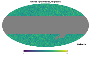
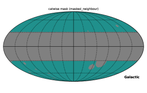
Figure 1: Left: Number count map and Right: the corresponding mask map for catWISE2020 catalogue after following the masking procedure described in the text.

3 Methodology

We are interested in studying the dipole signal in three observables (a) number counts $N$, (b) mean spectral index $\bar{\alpha}$ and (c) mean flux density $\bar{B}$. The dipole in number counts has already been studied earlier [18, 19]. In order to study the anisotropy in spectral index we consider the mean value of this variable in a small angular region. We use the Healpy pixelation scheme for our analysis. For a given pixel p we define the mean spectral index $\bar{\alpha}_{\mathrm{p}}$ as

$$\bar{\alpha}_{\mathrm{p}}=\frac{1}{N_{\mathrm{p}}}\sum_{i=1}^{N_{\mathrm{p}}}\alpha_{i,\mathrm{p}}$$ (3.1)

here $N_{\mathrm{p}}$ is the total number of sources and $\alpha_{i,\mathrm{p}}$ denotes the spectral index of $i$th source in pixel p. The sum is performed over all the sources in the pixel. Similarly we define the mean flux density $\bar{B}_{\mathrm{p}}$ in pixel p as

$$\bar{B}_{\mathrm{p}}=\dfrac{1}{N_{\mathrm{p}}}\sum_{i=1}^{N_{\mathrm{p}}}B_{i,\mathrm{p}}$$ (3.2)

with $B_{i,\mathrm{p}}$ denoting the flux density of $i$th source in pixel p. In order to extract the dipole signal we use two different procedures. The $\chi^{2}$ method is described below while the details of the Healpy [68, 69] method can be found in Appendix A.

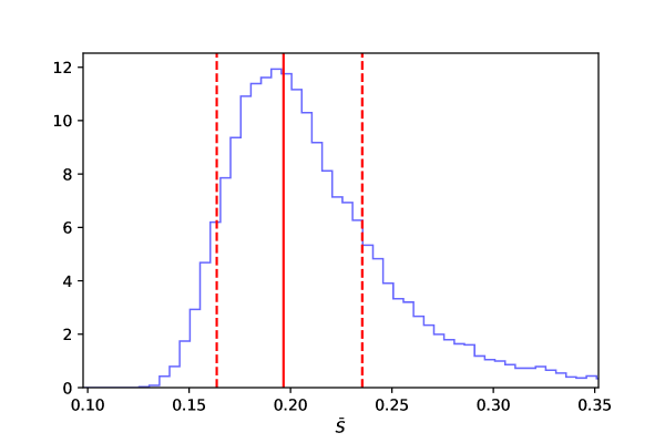
Figure 2: The mean flux density distribution for 50 sources, derived by sub-sampling the full catWISE2020 catalogue. The solid red line shows the median, and the dashed red lines are the one-$\sigma$ intervals around.

3.1 Multipole Expansion

Let $I(\theta,\phi)$ denote a generic quantity of interest ($N$, $\bar{\alpha}$ or $\bar{B}$) along the direction $(\theta,\phi)$. Assuming that multipoles $\ell\geq 3$ can be neglected, we write

$$I(\theta,\phi)=\mathcal{M}_{0}^{\mathrm{I}}+{\mathcal{D}}_{x}^{\mathrm{I}}x+{\mathcal{D}}_{y}^{\mathrm{I}}y+{\mathcal{D}}_{z}^{\mathrm{I}}z+{\mathcal{Q}}_{xy}^{\mathrm{I}}xy+{\mathcal{Q}}_{xz}^{\mathrm{I}}xz+{\mathcal{Q}}_{yz}^{\mathrm{I}}yz+{\mathcal{Q}}_{z^{2}}^{\mathrm{I}}(2z^{2}-x^{2}-y^{2})+{\mathcal{Q}}_{x^{2}-y^{2}}^{\mathrm{I}}(x^{2}-y^{2})$$ (3.3)

Above equation is basically the spherical harmonic decomposition in the Cartesian basis. Eq. (3.3) contains 9 coefficients–one for monopole ($\mathcal{M}_{0}$), three for dipole $(\mathcal{D}_{x},\mathcal{D}_{y},\mathcal{D}_{z})$, and five for quadrupole $(\mathcal{Q}_{xy},\mathcal{Q}_{xz},\mathcal{Q}_{yz},\mathcal{Q}_{z^{2}},\mathcal{Q}_{x^{2}-y^{2}})$, to be solved for. The superscript $I$ denotes the observable being considered.

The observed dipole for any of the observables $\mathbf{D}$ is related to the dipole components $\bm{\mathcal{D}}_{i}$ present in Eq. (3.3) as

$$|\mathbf{D}|={\sqrt{\mathcal{D}^{2}_{x}+\mathcal{D}^{2}_{y}+\mathcal{D}^{2}_{z}}\over\mathcal{M}_{0}}\,.$$ (3.4)

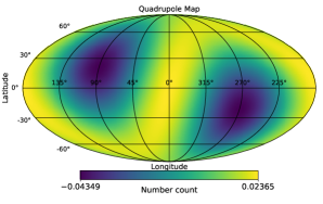
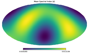
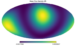
Figure 3: The extracted quadrupole for number counts $N$, mean spectral index $\bar{\alpha}$ and mean flux density $\bar{B}$ (anticlockwise from top left) in the Galactic coordinate system. It can be seen from the figure, the number counts quadrupole (top row left) broadly aligns with the ecliptic poles, indicating systematic bias.

3.2 The $\chi^{2}$ Statistic

In order to determine the coefficients of Eq. (3.3), we first divide the whole sky into equal-area pixels using python package Healpy and determine the quantity of interest $I_{\mathrm{p}}$ for the pixel p. Then we determine the coefficients in Eq. (3.3) using the $\chi^{2}$ minimization,

$$\chi^{2}=\sum_{\mathrm{p}=1}^{N_{\mathrm{t}}}\Bigg{[}\frac{I_{\mathrm{p}}-I(\theta,\phi)}{\sigma_{\mathrm{p}}^{\mathrm{I}}}\Bigg{]}^{2}$$ (3.5)

where $\sigma_{\mathrm{p}}^{\mathrm{I}}$ denotes the error in the observable $I_{\mathrm{p}}$ in a given pixel p, $N_{\mathrm{t}}$ is the number of unmasked pixels, and $I(\theta,\phi)$ is given in Eq. (3.3).

Although, the source number count follows the Poisson distribution, on account of a large number of sources in pixels, it approaches the Gaussian distribution. Thus for the number count map, for a pixel with $N_{\mathrm{p}}$ sources, we consider $\sigma_{\mathrm{p}}^{N}=\sqrt{N_{\mathrm{p}}}$. For observables $\bar{\alpha}$ and $\bar{B}$, the distribution is non-trivial and asymmetric. So to determine $\sigma_{\mathrm{p}}$ for these observables, we resort to sub-sampling. For a pixel with $n$ sources, we draw sub-samples with a number count $n$ from the full catWISE2020 catalogue. Next, we determine the $\bar{\alpha}$ or $\bar{B}$ of these sub-samples. The observed distribution for mean flux density is shown in Figure 2. We notice the skewness in distribution, and draw a $1\sigma$ confidence interval around the median and determine asymmetric error bars, i.e., $\sigma_{\mathrm{p}}^{(\pm)}$. Depending on whether the model’s predicted value is larger or smaller than the observed value, we choose $\sigma_{\mathrm{p}}^{\mathrm{I}}$ equal to $\sigma_{\mathrm{p}}^{(+)}$ or $\sigma_{\mathrm{p}}^{(-)}$ and perform $\chi^{2}$ minimization.

4 Results and Discussion

In this section, we give the results of multipole extraction for all three observables using the $\chi^{2}$ method. We apply our second method to number only, as it involves symmetric error bars (see §3.2).

4.1 Source Number Counts $N$

Using $\chi^{2}$ method, we find the dipole direction $(l,b)=(238.5^{\circ}\pm 7.8^{\circ},29.6^{\circ}\pm 5.8)$. This direction is quite close to the CMB dipole. On the other hand, the magnitude of the dipole is found to be $|\mathbf{D}|=0.017\pm 0.002$. This is much larger in comparison to the expected kinematic dipole and is consistent with the value found in [19] that was obtained by a different data analysis procedure. The extracted quadrupole in number counts is shown in Figure 3 (top row left). As we can see from the figure, it broadly aligns with the ecliptic poles, indicating systematic bias as already noted in [19]. In our procedure, we do not need to model this bias since the quadrupole is directly extracted from the data along with the dipole.

We now make a comparison of $\chi^{2}$ results with those obtained using Healpy. The details of the multipole extraction and error estimation can be found in Appendix A. The results are shown in Figure 4. These are the histograms of various multipole components obtained using 10,000 simulations. The dipole magnitude and directions are found to be $|\mathbf{D}|=0.016\pm 0.002$ and $(l,b)=(237.9^{\circ}\pm 8.4^{\circ},30.4^{\circ}\pm 5.0^{\circ})$ respectively. Thus we find the results of Healpy method are quite close to those obtained using $\chi^{2}$ method. We have also shown the dependence of extracted monopole $\mathcal{M}_{0}$ on the order of expansion (Eq. 3.3) in Table 1, using Healpy method.

It is important to ascertain that the values of extracted multipole components don’t depend upon the order to which we make the expansion in Eq. (3.3). To this end, we find that $\mathcal{M}_{0}$ shows no change after $\ell=2$. We ascribe this to the fact that beyond $\ell=2$, the multipole components are negligible.

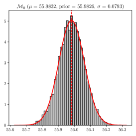
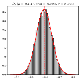
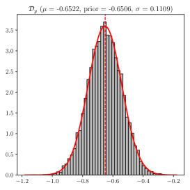
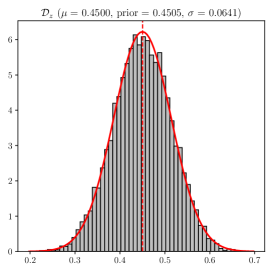
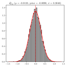
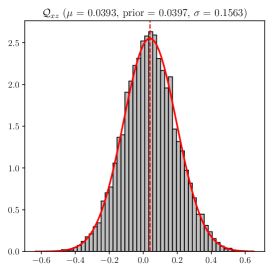
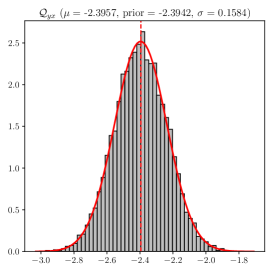
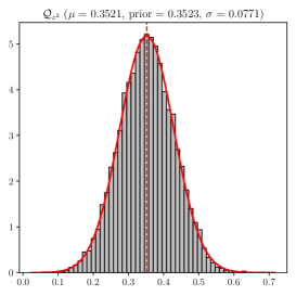
Figure 4: Distribution histogram of monopole, dipole and quadrupole components (Eq. 3.3) for source number counts $N$ obtained using Healpy method. In the plot, thick vertical dotted lines are priors and thick red curve is the Gaussian fit to the histogram. The corresponding mean ($\mu$) standard deviation ($\sigma$) are also shown in the corresponding titles.

	$\ell\leq 0$	$\ell\leq 1$	$\ell\leq 2$	$\ell\leq 3$
$\mathcal{M}_{0}$	$56.29$	$56.30$	$55.98$	$55.98$

Table 1: Comparison of the monopole values $\mathcal{M}_{0}$ in number counts by considering the expansion for various $\ell$ values. The monopole value shows no change after $\ell=2$.

4.2 Mean Spectral Index $\bar{\alpha}$

We find a significant signal of dipolar anisotropy in this observable. The dipole amplitude is found to be $0.0066\pm 0.0011$ and the direction $l=171^{\circ}\pm 6^{\circ}$ and $b=7^{\circ}\pm 6^{\circ}$. As discussed in §1, this observable does not get any contribution due to kinematic effects. Thus, the presence of anisotropy in this parameter indicates either a bias or a possible departure from the $\Lambda$CDM. We also find a very strong quadrupole in the data, roughly correlated with the ecliptic poles, as shown in Figure 3 (top row right). This may arise due to observational bias which is also present in number counts. The dipole direction lies close to the galactic plane and points roughly opposite to the galactic center, indicating a possible contamination from our galaxy. In order to study galactic and other sources of contamination in data, we study the effect of (a) flux cut ($S_{\mathrm{cut}}$) and (b) galactic cut ($b_{\mathrm{cut}}$) on this observable.

4.2.1 Effect of Flux Cut

We study the effect of flux cut $S<S_{\mathrm{cut}}$ as we change $S_{\mathrm{cut}}$ from $\infty$ to 0.1 mJy. The results are given in Table 2.

$S_{\mathrm{cut}}$ (mJy)	Sources	$f_{\mathrm{sky}}$	$|\mathbf{D}|$	$l$ (deg.)	$b$ (deg.)
$\infty$	$1307511$	$0.4724$	$0.0066\pm 0.00113$	$171\pm 6$	$7\pm 6$
$10.0$	$1307023$	$0.4724$	$0.0067\pm 0.00099$	$172\pm 5$	$9\pm 4$
$0.7$	$1263875$	$0.4722$	$0.0067\pm 0.00148$	$167\pm 9$	$8\pm 5$
$0.3$	$1120488$	$0.4721$	$0.0065\pm 0.00090$	$168\pm 12$	$10\pm 6$
$0.2$	$953664$	$0.4718$	$0.0064\pm 0.00071$	$172\pm 11$	$10\pm 4$
$0.1$	$302607$	$0.4647$	$0.0070\pm 0.00372$	$217\pm 43$	$22\pm 20$

Table 2: The dipole in mean spectral index $\bar{\alpha}$ as a function of flux cut $S<S_{\mathrm{cut}}$. It can be seen that the dipole amplitude as well as direction is almost consistent till the flux cut of 0.2 mJy. The dipole direction lies close to the galactic plane and points opposite to the galactic center. Beyond $S_{\mathrm{cut}}=0.2$, there is a drastic change in the number of sources, leading to drastic changes in the magnitude, direction and significance of the dipole.

$b_{\mathrm{cut}}$ (deg.)	Sources	$f_{\mathrm{sky}}$	$|\mathbf{D}|$	$l$ (deg.)	$b$ (deg.)
$30$	$1307511$	$0.4724$	$0.0066\pm 0.00113$	$171\pm 6$	$7\pm 6$
$35$	$1117078$	$0.4030$	$0.0074\pm 0.00147$	$161\pm 9$	$5\pm 6$
$40$	$950186$	$0.3426$	$0.0055\pm 0.00099$	$172\pm 14$	$4\pm 5$
$45$	$767093$	$0.2765$	$0.0054\pm 0.00135$	$150\pm 14$	$7\pm 10$
$50$	$619814$	$0.2235$	$0.0036\pm 0.00184$	$147\pm 26$	$14\pm 15$

Table 3: The dipole in mean spectral index $\bar{\alpha}$ as a function of galactic cut. This means we have considered those sources with $|b|>b_{\mathrm{cut}}$. The number of sources decrease very rapidly leading to decrease in significance as the cut is increased.

From the table we observe that

1. Both dipole amplitude and the direction remains almost constant till $S_{\mathrm{cut}}=0.2$ mJy.

2. At 0.1 mJy cut, the error in both the the magnitude and the direction increases considerably. This can be attributed to the drastic change in the number of sources from 953,664 to 302,607 as we go from 0.2 to 0.1 mJy. However, within errors, the result remains the same as with other less stringent flux cuts.

4.2.2 Effect of Galactic Cut

The dipole direction in the mean spectral index is found to be close to the galactic plane, indicating galactic contamination. To explore this further, we study the effect of galactic cut on the observable. This is depicted in Table 3. From the table we can observe the following

1. For the galactic cut $30^{\circ}\leq b_{\mathrm{cut}}\leq 45^{\circ}$, we find a very significant dipole signal. The significance is considerably reduced for more stringent galactic cuts $b_{\mathrm{cut}}\leq 50^{\circ}$. The direction for all the cuts in the range $30^{\circ}\leq b_{\mathrm{cut}}\leq 40^{\circ}$ agrees within errors. It deviates as we impose a more stringent cut $b_{\mathrm{cut}}\geq 45^{\circ}$, but the deviation is not very significant.

2. The effect is not significant for more stringent galactic cuts such as $b_{\mathrm{cut}}>50^{\circ}$.

Since the effect persists for a wide range of flux cuts, so we cannot attribute it to a few bright sources. The fact that it points roughly opposite to the galactic center indicates contamination from the galaxy. Hence, it is reasonable to attribute the observed dipole to galactic bias and conclude that the current data is consistent with isotropy in this variable.

4.3 Mean Flux Density $\bar{B}$

Here also we study the effect of flux and galactic cuts on the dipole.

4.3.1 Effect of Flux Cut

For the flux cuts, the results are summarised in Table 4. From this table, we observe the following

1. The dipole significance suddenly drops after $S_{\mathrm{cut}}=10$ mJy. This indicates that the dipole signal can be attributed to very bright sources

2. For the cases when the dipole is significant (first two rows), the dipole lies in the galactic plane pointing towards the galactic center

3. In all other cases, the dipole points away from the plane and its significance also reduces

4.3.2 Effect of Galactic Cut

These results are given in Table 5. From the table, we find that

1. For galactic cuts $b_{\mathrm{cut}}\leq 40$, the dipole is significant. After this, the significance reduces considerably

2. For all flux cuts, the dipole points approximately towards galactic center

3. Except $b_{\mathrm{cut}}=45^{\circ}$ cut, the dipole lies close to the galactic plane

The results clearly suggest that dipole can be attributed to a few bright sources. Furthermore it may get contribution due to galactic contamination.

$S_{\mathrm{cut}}$ (mJy)	Sources	$f_{\mathrm{sky}}$	$|\mathbf{D}|$	$l$ (deg.)	$b$ (deg.)
$\infty$	$1307511$	$0.4724$	$0.01205\pm 0.003026$	$352\pm 60$	$10\pm 8$
$10.0$	$1307023$	$0.4724$	$0.00815\pm 0.001723$	$356\pm 16$	$11\pm 17$
$1.0$	$1284744$	$0.4724$	$0.00289\pm 0.001281$	$354\pm 78$	$38\pm 27$
$0.7$	$1263875$	$0.4722$	$0.00231\pm 0.000895$	$306\pm 89$	$65\pm 59$
$0.3$	$1120488$	$0.4721$	$0.00192\pm 0.000906$	$355\pm 39$	$42\pm 46$
$0.2$	$953664$	$0.4718$	$0.00062\pm 0.000544$	$304\pm 93$	$32\pm 39$
$0.1$	$302607$	$0.4647$	$0.00092\pm 0.000421$	$66\pm 53$	$-14\pm 17$

Table 4: The dipole parameters obtained using the quadrupole $\chi^{2}$ method for $\bar{B}$. The values in the first column indicate that only sources with flux less than the flux cuts are considered. The second column and the third columns are the number of sources left and sky fraction after applying the flux cut.

$b_{\mathrm{cut}}$ (deg.)	Sources	$f_{\mathrm{sky}}$	$|\mathbf{D}|$	$l$ (deg.)	$b$ (deg.)
$30$	$1307511$	$0.4724$	$0.0121\pm 0.00303$	$352\pm 60$	$10\pm 8$
$35$	$1117078$	$0.4030$	$0.0151\pm 0.00165$	$357\pm 2$	$7\pm 2$
$40$	$950186$	$0.3426$	$0.0104\pm 0.00177$	$23\pm 8$	$18\pm 5$
$45$	$767093$	$0.2765$	$0.0045\pm 0.00175$	$351\pm 149$	$37\pm 22$
$50$	$619814$	$0.2235$	$0.0136\pm 0.01535$	$304\pm 53$	$21\pm 35$

Table 5: The dipole in mean flux density $\bar{B}$ as a function of galactic cut. Whenever the dipole is significant, the direction lies close to the galactic plane pointing towards galactic center.

5 Conclusion and Outlook

In this paper, we have studied the dipole in three observables — source number counts, mean spectral index, and mean flux density. We have used two different data analysis methods ($\chi^{2}$ and Healpy) which directly extract the first three multipoles ($\ell=0,1,2$) and the corresponding errors from the data. The higher multipoles are neglected since they are found to be small. The Healpy method is applied only for number counts as it involves symmetric error bars. We find results obtained using both methods almost the same. Further, these values are found to be consistent with [18]. This provides an independent check on their results. We point out that in our case, we do not model the bias in data associated with the ecliptic pole. This bias leads to a strong quadrupole and is directly extracted from data.

Although the observable $N$ has symmetric error bars, this is no longer true for $\bar{\alpha}$ and $\bar{B}$. Thus we have used only $\chi^{2}$ method for these observables. Generalization of the Healpy method to the non-symmetric error bars can be pursued in future. We find a very strong signal of dipole anisotropy in the mean spectral index $\bar{\alpha}$. The direction in this case lies close to the galactic plane and points roughly opposite to the galactic center. Hence to evaluate the effect of galactic contamination, we study the dipolar anisotropy as a function of the galactic cut. We find that the signal remains very significant for galactic cut $b_{\mathrm{cut}}>45^{\circ}$ but starts to loose significance for more stringent cuts. We also study the effect of flux cuts $S<S_{\mathrm{cut}}$. We find that both the amplitude and direction of the dipole don’t show much change as the flux cut is made more stringent. However, as expected, the errors in the dipole parameters become very large for the very stringent flux cut of $S_{\mathrm{cut}}$ = 0.1 mJy. Since the dipole in this variable points roughly opposite to the galactic center, we conclude that it may be attributed to contamination from our galaxy. This variable also shows a strong quadrupole roughly correlated with the ecliptic poles, which may indicate the presence of observational bias in data similar to that present in number counts.

The mean flux density $\bar{B}$ also shows a significant dipole with direction pointing towards the galactic center. The dipole becomes considerably reduced and also doesn’t remain significant if we impose the flux cut $S_{\mathrm{cut}}<1$ mJy. Additionally, the significance of the dipole reduces beyond the galactic cut $b_{\mathrm{cut}}\leq 40^{\circ}$. Hence it is reasonable to attribute the observed dipole in this variable to a few bright sources. In conclusion, both the mean spectral index and the mean flux density are consistent with isotropy.

Appendix A An alternative method for extracting masked sky multipole coefficients

In this section, we give details of an alternate procedure to extract the multipole coefficients for a given observable. Here, we have applied the method only for number counts map $N$. First, we talk about extracting the coefficients and then a method for estimating the corresponding errors. In order to better understand the modus operandi, we have considered some special cases. We have also given an example of our procedure in Figure 4 that shows the distribution of various parameters which is found to be Gaussian to a very good extend. Additionally, we have given corresponding mean values ($\mu$) and standard deviation ($\sigma$) for number counts $N$.

A.1 Coefficients’ Extraction

The method is based on solving a system of linear equations. In a multipole expansion, considered till $\ell$, we’d need $(\ell+1)^{2}$ equations for obtaining all the coefficients in Eq. (3.3). Thus in our case, we need to solve a system of 9 linear equations. Although, in our analysis, we have terminated the expansion at $\ell=2$, yet we must emphasize that the procedure can be generalized to any order. As the first step, we write the discretized version of Eq. (3.3) (here $r_{\mathrm{p}}^{2}=x_{\mathrm{p}}^{2}+y_{\mathrm{p}}^{2}+z_{\mathrm{p}}^{2}$)

$$I_{\mathrm{p}} = \mathcal{M}_{0}^{\mathrm{I}}+\mathcal{D}_{x}^{\mathrm{I}}\,x_{\mathrm{p}}+\mathcal{D}_{y}^{\mathrm{I}}\,y_{\mathrm{p}}+\mathcal{D}_{z}^{\mathrm{I}}\,z_{\mathrm{p}}+\mathcal{Q}_{xy}^{\mathrm{I}}\,x_{\mathrm{p}}y_{\mathrm{p}}+\mathcal{Q}_{xz}^{\mathrm{I}}\,x_{\mathrm{p}}z_{\mathrm{p}}$$ (A.1)

$$+ \mathcal{Q}_{yz}^{\mathrm{I}}\,y_{\mathrm{p}}z_{\mathrm{p}}+\mathcal{Q}_{z^{2}}^{\mathrm{I}}\,(3z^{2}_{\mathrm{p}}-r^{2}_{\mathrm{p}})+\mathcal{Q}_{x^{2}-y^{2}}^{\mathrm{I}}\,(x^{2}_{\mathrm{p}}-y^{2}_{\mathrm{p}})$$

In this equation, $I_{\mathrm{p}}$ and $(x_{\mathrm{p}},y_{\mathrm{p}},z_{\mathrm{p}})$ respectively denote the observable value and cartesian coordinates of the given pixel in the Healpy pixelation scheme. For obtaining these coefficients, we now set up a system of linear equations. To get our first equation, we sum over all the unmasked pixels $N_{\mathrm{t}}$ on both sides to get

$$\sum_{\mathrm{p}=1}^{N_{\mathrm{t}}}I_{\mathrm{p}} = \mathcal{M}_{0}^{\mathrm{I}}\sum_{\mathrm{p}=1}^{N_{\mathrm{t}}}1+\mathcal{D}_{x}^{\mathrm{I}}\sum_{\mathrm{p}=1}^{N_{\mathrm{t}}}x_{\mathrm{p}}+\mathcal{D}_{y}^{\mathrm{I}}\sum_{\mathrm{p}=1}^{N_{\mathrm{t}}}y_{\mathrm{p}}+\mathcal{D}_{z}^{\mathrm{I}}\sum_{\mathrm{p}=1}^{N_{\mathrm{t}}}z_{\mathrm{p}}+\mathcal{Q}_{xy}^{\mathrm{I}}\sum_{\mathrm{p}=1}^{N_{\mathrm{t}}}x_{\mathrm{p}}y_{\mathrm{p}}+\mathcal{Q}_{xz}^{\mathrm{I}}\sum_{\mathrm{p}=1}^{N_{\mathrm{t}}}x_{\mathrm{p}}z_{\mathrm{p}}$$ (A.2)

$$+ \mathcal{Q}_{yz}^{\mathrm{I}}\sum_{\mathrm{p}=1}^{N_{\mathrm{t}}}y_{\mathrm{p}}z_{\mathrm{p}}+\mathcal{Q}_{z^{2}}^{\mathrm{I}}\sum_{\mathrm{p}=1}^{N_{\mathrm{t}}}(3z^{2}_{\mathrm{p}}-r^{2}_{\mathrm{p}})+\mathcal{Q}_{x^{2}-y^{2}}^{\mathrm{I}}\sum_{\mathrm{p}=1}^{N_{\mathrm{t}}}(x^{2}_{\mathrm{p}}-y^{2}_{\mathrm{p}})$$

To get the next equation, we multiply (A.1) by $x_{\mathrm{p}}$ and then perform the sum. We repeat this process, by multiplying next with $y_{\mathrm{p}}$ and so on, i.e., all the direction dependent factors, multiplying multipole coefficients in Eq. (A.1). Finally, we get a system of 9 linear equations which can be written as

$$\mathbb{M}\,\mathbb{P}=\mathbb{N}$$ (A.3)

here the parameter vector $\mathbb{P}$ is

$$\mathbb{P}=\big{[}\mathcal{M}_{0}^{\mathrm{I}}\ \mathcal{D}_{x}^{\mathrm{I}}\ \mathcal{D}_{y}^{\mathrm{I}}\ \mathcal{D}_{z}^{\mathrm{I}}\ \mathcal{Q}_{xy}^{\mathrm{I}}\ \mathcal{Q}_{xz}^{\mathrm{I}}\ \mathcal{Q}_{yz}^{\mathrm{I}}\ \mathcal{Q}_{z^{2}}^{\mathrm{I}}\ \mathcal{Q}_{x^{2}-y^{2}}^{\mathrm{I}}\big{]}^{T}$$ (A.4)

and $T$ in the superscript denotes the transpose. The vector $\mathbb{N}$ on the RHS is given by

$$\mathbb{N}=\Bigg{[}\sum_{\mathrm{p}}^{N_{\mathrm{t}}}(I_{\mathrm{p}}\ I_{\mathrm{p}}x_{\mathrm{p}}\ I_{\mathrm{p}}y_{\mathrm{p}}\ I_{\mathrm{p}}z_{\mathrm{p}}\ I_{\mathrm{p}}x_{\mathrm{p}}y_{\mathrm{p}}\ I_{\mathrm{p}}x_{\mathrm{p}}x_{\mathrm{p}}\ I_{\mathrm{p}}y_{\mathrm{p}}z_{\mathrm{p}}\ I_{\mathrm{p}}Z_{\mathrm{p}}\ I_{\mathrm{p}}M_{\mathrm{p}})\Bigg{]}^{T}$$ (A.5)

where for brevity sake we have defined $Z_{\mathrm{p}}=3z_{\mathrm{p}}^{2}-1$, $M_{\mathrm{p}}=x_{\mathrm{p}}^{2}-y_{\mathrm{p}}^{2}$ and the sum outside the parenthesis is meant to be performed on all the terms inside the parenthesis over pixel p. Finally, the symmetric matrix $\mathbb{M}$ is given by the following expression

$$\mathbb{M}=\sum_{\mathrm{p}}^{N_{\mathrm{t}}}\begin{bmatrix}1&x_{\mathrm{p}}&y_{\mathrm{p}}&z_{\mathrm{p}}&x_{\mathrm{p}}y_{\mathrm{p}}&x_{\mathrm{p}}z_{\mathrm{p}}&y_{\mathrm{p}}z_{\mathrm{p}}&Z_{\mathrm{p}}&M_{\mathrm{p}}\\ x_{\mathrm{p}}&x_{\mathrm{p}}^{2}&x_{\mathrm{p}}y_{\mathrm{p}}&x_{\mathrm{p}}z_{\mathrm{p}}&x_{\mathrm{p}}^{2}y_{\mathrm{p}}&x_{\mathrm{p}}^{2}z_{\mathrm{p}}&x_{\mathrm{p}}y_{\mathrm{p}}z_{\mathrm{p}}&x_{\mathrm{p}}Z_{\mathrm{p}}&x_{\mathrm{p}}M_{\mathrm{p}}\\ y_{\mathrm{p}}&x_{\mathrm{p}}y_{\mathrm{p}}&y_{\mathrm{p}}^{2}&y_{\mathrm{p}}z_{\mathrm{p}}&x_{\mathrm{p}}y_{\mathrm{p}}^{2}&x_{\mathrm{p}}y_{\mathrm{p}}z_{\mathrm{p}}&y_{\mathrm{p}}^{2}z_{\mathrm{p}}&y_{\mathrm{p}}Z_{\mathrm{p}}&M_{\mathrm{p}}\\ z_{\mathrm{p}}&x_{\mathrm{p}}z_{\mathrm{p}}&y_{\mathrm{p}}z_{\mathrm{p}}&z_{\mathrm{p}}^{2}&x_{\mathrm{p}}y_{\mathrm{p}}z_{\mathrm{p}}&x_{\mathrm{p}}z_{\mathrm{p}}&y_{\mathrm{p}}z_{\mathrm{p}}^{2}&z_{\mathrm{p}}Z_{\mathrm{p}}&z_{\mathrm{p}}M_{\mathrm{p}}\\ x_{\mathrm{p}}y_{\mathrm{p}}&x_{\mathrm{p}}^{2}y_{\mathrm{p}}&x_{\mathrm{p}}y_{\mathrm{p}}^{2}&x_{\mathrm{p}}y_{\mathrm{p}}z_{\mathrm{p}}&(x_{\mathrm{p}}y_{\mathrm{p}})^{2}&x_{\mathrm{p}}^{2}y_{\mathrm{p}}z_{\mathrm{p}}&x_{\mathrm{p}}y_{\mathrm{p}}^{2}z_{\mathrm{p}}&x_{\mathrm{p}}y_{\mathrm{p}}Z_{\mathrm{p}}&x_{\mathrm{p}}y_{\mathrm{p}}M_{\mathrm{p}}\\ x_{\mathrm{p}}z_{\mathrm{p}}&x_{\mathrm{p}}^{2}z_{\mathrm{p}}&x_{\mathrm{p}}y_{\mathrm{p}}z_{\mathrm{p}}&x_{\mathrm{p}}z_{\mathrm{p}}^{2}&x_{\mathrm{p}}^{2}y_{\mathrm{p}}z_{\mathrm{p}}&(x_{\mathrm{p}}z_{\mathrm{p}})^{2}&x_{\mathrm{p}}y_{\mathrm{p}}z_{\mathrm{p}}^{2}&x_{\mathrm{p}}z_{\mathrm{p}}Z_{\mathrm{p}}&x_{\mathrm{p}}z_{\mathrm{p}}M_{\mathrm{p}}\\ y_{\mathrm{p}}z_{\mathrm{p}}&x_{\mathrm{p}}y_{\mathrm{p}}z_{\mathrm{p}}&y_{\mathrm{p}}^{2}z_{\mathrm{p}}&y_{\mathrm{p}}z_{\mathrm{p}}^{2}&x_{\mathrm{p}}y_{\mathrm{p}}^{2}z_{\mathrm{p}}&x_{\mathrm{p}}y_{\mathrm{p}}z_{\mathrm{p}}^{2}&(y_{\mathrm{p}}z_{\mathrm{p}})^{2}&y_{\mathrm{p}}z_{\mathrm{p}}Z_{\mathrm{p}}&y_{\mathrm{p}}z_{\mathrm{p}}M_{\mathrm{p}}\\ Z_{\mathrm{p}}&x_{\mathrm{p}}Z_{\mathrm{p}}&y_{\mathrm{p}}Z_{\mathrm{p}}&z_{\mathrm{p}}Z_{\mathrm{p}}&x_{\mathrm{p}}y_{\mathrm{p}}Z_{\mathrm{p}}&x_{\mathrm{p}}z_{\mathrm{p}}&y_{\mathrm{p}}z_{\mathrm{p}}Z_{\mathrm{p}}&Z_{\mathrm{p}}^{2}&M_{\mathrm{p}}Z_{\mathrm{p}}\\ M_{\mathrm{p}}&x_{\mathrm{p}}M_{\mathrm{p}}&y_{\mathrm{p}}M_{\mathrm{p}}&z_{\mathrm{p}}M_{\mathrm{p}}&x_{\mathrm{p}}y_{\mathrm{p}}M_{\mathrm{p}}&x_{\mathrm{p}}z_{\mathrm{p}}M_{\mathrm{p}}&y_{\mathrm{p}}z_{\mathrm{p}}M_{\mathrm{p}}&M_{\mathrm{p}}Z_{\mathrm{p}}&M_{\mathrm{p}}^{2}\end{bmatrix}$$ (A.6)

A.2 Some Special Cases

In order to gain some insights about the modus operandi, it would be useful to consider some special cases. First we analyze what happens when no pixel is masked. In that case it can be shown that the matrix in Eq. (A.6) becomes diagonal. This is a consequence of the fact that when no pixel is masked

$$\sum_{\text{all pixels }}x^{a}_{\mathrm{p}}y^{b}_{\mathrm{p}}z^{c}_{\mathrm{p}}=0$$ (A.7)

when either $a$, $b$ or $c$ are odd. This further implies that when we have full sky information available then all the multipole parameters can be determined independently. But in reality, we always have a masked sky. In that case, the parameter extraction will depend upon where the series truncates. Thus in principle infinite number of parameters would be needed. But as we have seen that beyond quadrupole the power is small hence we truncated our series at $\ell=2$. We have also checked the effect of parameter extraction and $\ell$ value at which the series is terminated. These results are shown for monopole in Table 1.

Since the method is dependent upon information in unmasked pixels, we can in principle extract information in an extreme case when only one pixel information is available. But in reality we found that the method at NSide=64 becomes unstable when we have information available in $\lesssim 10$ pixels. Additionally, we have also checked that the method works extremely well and calculates same values of the fitting parameters when we randomly mask the pixels.

A.3 Error Estimation

In order to estimate the errors in the fitted parameters, we perform simulations using the following algorithm, summarized in Figure 5.

1. Full Sky Map: The monopole, dipole and quadrupole components from the data map are extracted using Eq. (A.3). These multipoles are then used to prepare a full sky map $\mathbb{F}$ at NSIDE 64

2. Simulated Maps: To incorporate error, we add, to the data value $N_{\mathrm{p}}$ of pixel p, a random number generated from the Poisson distribution using numpy.random.poisson$(N_{\mathrm{p}})$. This gives a simulated map $\mathbb{S}_{j}$. From this we again extract multipoles using Eq. (A.3).

3. The previous step is repeated 10,000 times which gives a distribution for various extracted multipoles. The distribution, which is found to be Gaussian, is given in Figure 4. From this distribution, we can calculate relevant quantities of interest – $\mu$ and $\sigma$.

Figure 5: Algorithm for generating mock maps and multipole extraction for number counts $N$. For details, the reader is referred to §A.3.

References

- [1] C. A. P. Bengaly, R. Maartens and M. G. Santos, Probing the Cosmological Principle in the counts of radio galaxies at different frequencies, JCAP 1804 (2018) 031 [1710.08804].
- [2] T. Nadolny, R. Durrer, M. Kunz and H. Padmanabhan, A new way to test the Cosmological Principle: measuring our peculiar velocity and the large-scale anisotropy independently, JCAP 11 (2021) 009 [2106.05284].
- [3] Y. Kim, C.-G. Park, H. Noh and J.-c. Hwang, CMASS galaxy sample and the ontological status of the cosmological principle, Astron. Astrophys. 660 (2022) A139 [2112.04134].
- [4] C. Bengaly, A null test of the Cosmological Principle with BAO measurements, Phys. Dark Univ. 35 (2022) 100966 [2111.06869].
- [5] O. Lahav, Observational tests for the cosmological principle and world models, NATO Sci. Ser. C 565 (2001) 131 [astro-ph/0001061].
- [6] P. K. Aluri et al., Is the Observable Universe Consistent with the Cosmological Principle?, 2207.05765.
- [7] S. Ghosh, P. Jain, G. Kashyap, R. Kothari, S. Nadkarni-Ghosh and P. Tiwari, Probing statistical isotropy of cosmological radio sources using square kilometre array, Journal of Astrophysics and Astronomy 37 (2016) 1.
- [8] C. A. P. Bengaly, R. Maartens, N. Randriamiarinarivo and A. Baloyi, Testing the Cosmological Principle in the radio sky, JCAP 09 (2019) 025 [1905.12378].
- [9] S. Weinberg, Cosmology. Oxford University Press, 2008.
- [10] N. Horstmann, Y. Pietschke and D. J. Schwarz, Inference of the cosmic rest-frame from supernovae Ia, 2111.03055.
- [11] A. Kogut, C. Lineweaver, G. F. Smoot, C. L. Bennett, A. Banday et al., Dipole anisotropy in the cobe differential microwave radiometers first-year sky maps, ApJ 419 (1993) 1 [astro-ph/9312056].
- [12] G. Hinshaw, J. L. Weiland, R. S. Hill, N. Odegard, C. Larson et al., Five-Year Wilkinson Microwave Anisotropy Probe Observations: Data Processing, Sky Maps, and Basic Results, ApJS 180 (2009) 225 [0803.0732].
- [13] J. Darling, The Universe is Brighter in the Direction of Our Motion: Galaxy Counts and Fluxes are Consistent with the CMB Dipole, 2205.06880.
- [14] A. K. Singal, Large Peculiar Motion of the Solar System from the Dipole Anisotropy in Sky Brightness due to Distant Radio Sources, ApJL 742 (2011) L23 [1110.6260].
- [15] C. Gibelyou and D. Huterer, Dipoles in the Sky, MNRAS 427 (2012) 1994 [1205.6476].
- [16] M. Rubart and D. J. Schwarz, Cosmic radio dipole from nvss and wenss, A&A 555 (2013) [1301.5559].
- [17] P. Tiwari, R. Kothari, A. Naskar, S. Nadkarni-Ghosh and P. Jain, Dipole anisotropy in sky brightness and source count distribution in radio NVSS data, Astroparticle Physics 61 (2015) 1 [1307.1947].
- [18] N. J. Secrest, S. von Hausegger, M. Rameez, R. Mohayaee, S. Sarkar and J. Colin, A Test of the Cosmological Principle with Quasars, Astrophys. J. Lett. 908 (2021) L51 [2009.14826].
- [19] N. Secrest, S. von Hausegger, M. Rameez, R. Mohayaee and S. Sarkar, A Challenge to the Standard Cosmological Model, 2206.05624.
- [20] C. Blake and J. Wall, Measurement of the angular correlation function of radio galaxies from the NRAO VLA Sky Survey, Monthly Notices of the Royal Astronomical Society 329 (2002) L37 [astro-ph/0111328].
- [21] P. Tiwari and P. Jain, Dipole anisotropy in integrated linearly polarized flux density in NVSS data, Monthly Notices of the Royal Astronomical Society 447 (2015) 2658 [1308.3970].
- [22] C.-G. Park, H. Hyun, H. Noh and J.-c. Hwang, The cosmological principle is not in the sky, Mon. Not. Roy. Astron. Soc. 469 (2017) 1924 [1611.02139].
- [23] H. Eriksen, F. Hansen, A. Banday, K. Goŕski and P. Lilje, Asymmetries in the Cosmic Microwave Background anisotropy field, ApJ 605 (2004) 14 [astro-ph/0307507].
- [24] H. K. Eriksen, A. J. Banday, K. M. Górski, F. K. Hansen and P. B. Lilje, Hemispherical Power Asymmetry in the Third-Year Wilkinson Microwave Anisotropy Probe Sky Maps, ApJL 660 (2007) L81 [astro-ph/0701089].
- [25] Planck Collaboration, Akrami, Y., Ashdown, M., Aumont, J., Baccigalupi, C., Ballardini, M. et al., Planck 2018 results - vii. isotropy and statistics of the cmb, A&A 641 (2020) A7.
- [26] Planck Collaboration, P. A. R. Ade, N. Aghanim, Y. Akrami, P. K. Aluri, M. Arnaud et al., Planck 2015 results. XVI. Isotropy and statistics of the CMB, A&A 594 (2016) A16 [1506.07135].
- [27] Planck Collaboration, P. A. R. Ade, N. Aghanim, C. Armitage-Caplan, M. Arnaud, M. Ashdown et al., Planck 2013 results. XXIII. Isotropy and statistics of the CMB, A&A 571 (2014) A23 [1303.5083].
- [28] J. Hoftuft, H. K. Eriksen, A. J. Banday, K. M. Gorski, F. K. Hansen and P. B. Lilje, Increasing evidence for hemispherical power asymmetry in the five-year WMAP data, Astrophys. J. 699 (2009) 985 [0903.1229].
- [29] J. P. Ralston and P. Jain, The Virgo alignment puzzle in propagation of radiation on cosmological scales, IJMPD 13 (2004) 1857 [astro-ph/0311430].
- [30] P. Jain and J. P. Ralston, Anisotropy in the propagation of radio polarizations from cosmologically distant galaxies, MPLA 14 (1999) 417.
- [31] A. de Oliveira-Costa, M. Tegmark, M. Zaldarriaga and A. Hamilton, Significance of the largest scale CMB fluctuations in WMAP, Physical Review D. 69 (2004) 063516 [astro-ph/0307282].
- [32] D. J. Schwarz, G. D. Starkman, D. Huterer and C. J. Copi, Is the low- microwave background cosmic?, PhRvL 93 (2004) 221301.
- [33] D. Hutsemékers, Evidence for very large-scale coherent orientations of quasar polarization vectors, A&A 332 (1998) 410.
- [34] P. Jain, G. Narain and S. Sarala, Large-scale alignment of optical polarizations from distant QSOs using coordinate-invariant statistics, MNRAS 347 (2004) 394.
- [35] P. Jain, S. Panda and S. Sarala, Electromagnetic polarization effects due to axion-photon mixing, PhRvD 66 (2002) 085007.
- [36] J. A. Morales and D. Saez, Evolution of polarization orientations in a flat universe with vector perturbations: CMB and quasistellar objects, Phys. Rev. D75 (2007) 043011 [astro-ph/0701914].
- [37] F. R. Urban and A. R. Zhitnitsky, Large-Scale Magnetic Fields, Dark Energy and QCD, Phys. Rev. D82 (2010) 043524 [0912.3248].
- [38] M. Yu. Piotrovich, Yu. N. Gnedin and T. M. Natsvlishvili, Coupling constant for axion and electromagnetic fields and cosmological observations, Astrophysics 52 (2009) 451.
- [39] N. Agarwal, A. Kamal and P. Jain, Alignments in quasar polarizations: Pseudoscalar-photon mixing in the presence of correlated magnetic fields, Phys. Rev. D83 (2011) 065014 [0911.0429].
- [40] R. Poltis and D. Stojkovic, Can primordial magnetic fields seeded by electroweak strings cause an alignment of quasar axes on cosmological scales?, Phys. Rev. Lett. 105 (2010) 161301 [1004.2704].
- [41] E. Hackmann, B. Hartmann, C. Lammerzahl and P. Sirimachan, Test particle motion in the space-time of a Kerr black hole pierced by a cosmic string, Phys. Rev. D82 (2010) 044024 [1006.1761].
- [42] N. Agarwal, P. K. Aluri, P. Jain, U. Khanna and P. Tiwari, A complete 3D numerical study of the effects of pseudoscalar-photon mixing on quasar polarizations, EPJC 72 (2012) 15 [1108.3400].
- [43] P. Tiwari and P. Jain, Extracting the spectral index of the intergalactic magnetic field from radio polarizations, Monthly Notices of the Royal Astronomical Society 460 (2016) 2698 [1505.00779].
- [44] P. Tiwari and P. Jain, A mechanism to explain galaxy alignment over a range of scales, Mon. Not. Roy. Astron. Soc. 513 (2022) 604 [2108.05011].
- [45] C. Gordon, W. Hu, D. Huterer and T. Crawford, Spontaneous isotropy breaking: A mechanism for CMB multipole alignments, Physical Review D. 72 (2005) 103002 [astro-ph/0509301].
- [46] A. L. Erickcek, S. M. Carroll and M. Kamionkowski, Superhorizon perturbations and the cosmic microwave background, Physical Review D. 78 (2008) 083012 [0808.1570].
- [47] L. P. Grishchuk and I. B. Zeldovich, Long-wavelength perturbations of a Friedmann universe, and anisotropy of the microwave background radiation, AZh 55 (1978) 209.
- [48] L. P. Grishchuk and I. B. Zeldovich, Long-wavelength perturbations of a Friedmann universe, and anisotropy of the microwave background radiation, Soviet Ast. 22 (1978) 125.
- [49] S. Ghosh, Generating Intrinsic Dipole Anisotropy in the Large Scale Structures, Physical Review D. 89 (2014) 063518 [1309.6547].
- [50] K. K. Das, K. Sankharva and P. Jain, Explaining excess dipole in NVSS data using superhorizon perturbation, JCAP 2021 (2021) 035 [2101.11016].
- [51] P. Tiwari, R. Kothari and P. Jain, Superhorizon perturbations: A possible explanation of the Hubble–Lemaître Tension and the Large Scale Anisotropy of the Universe, The Astrophysical Journal Letters 924 (2022) L36 [2111.02685].
- [52] P. K. Aluri and P. Jain, Large Scale Anisotropy due to Pre-Inflationary Phase of Cosmic Evolution, Modern Physics Letters A 27 (2012) 50014 [1108.3643].
- [53] P. Rath, T. Mudholkar, P. Jain, P. Aluri and S. Panda, Direction dependence of the power spectrum and its effect on the cosmic microwave background radiation, Journal of Cosmology and Astroparticle Physics 4 (2013) 7 [1302.2706].
- [54] C. B. Collins and S. W. Hawking, Why is the Universe isotropic?, Astrophys. J. 180 (1973) 317.
- [55] R. M. Wald, , PhRvD 28 (1983) 2118R.
- [56] C. B. Collins, Global structure of the Kantowski-Sachs cosmological models, J. Math. Phys. 18 (1977) 2116.
- [57] M. S. Turner and L. M. Widrow, Homogeneous Cosmological Models and New Inflation, Phys. Rev. Lett. 57 (1986) 2237.
- [58] G. Leon and E. N. Saridakis, Dynamics of the anisotropic Kantowsky-Sachs geometries in gravity, Class. Quant. Grav. 28 (2011) 065008 [1007.3956].
- [59] C. R. Fadragas, G. Leon and E. N. Saridakis, Dynamical analysis of anisotropic scalar-field cosmologies for a wide range of potentials, Class. Quant. Grav. 31 (2014) 075018 [1308.1658].
- [60] J. A. Stein-Schabes, Inflation in Spherically Symmetric Inhomogeneous Models, Phys. Rev. D 35 (1987) 2345.
- [61] L. G. Jensen and J. A. Stein-Schabes, A No Hair Theorem for Inhomogeneous Cosmologies, in International School of Particle Astrophysics: Gauge Theory and the Early Universe, pp. 0343–352, 3, 1986, DOI.
- [62] G. F. R. Ellis and J. E. Baldwin, On the expected anisotropy of radio source counts, MNRAS 206 (1984) 377.
- [63] P. Tiwari, S. Ghosh and P. Jain, The galaxy power spectrum from TGSS ADR1 and the effect of flux calibration systematics, Astrophys. J. 887 (2019) 175 [1907.10305].
- [64] E. L. Wright, P. R. M. Eisenhardt, A. K. Mainzer, M. E. Ressler, R. M. Cutri, T. Jarrett et al., The Wide-field Infrared Survey Explorer (WISE): Mission Description and Initial On-orbit Performance, AJ 140 (2010) 1868 [1008.0031].
- [65] P. R. M. Eisenhardt, F. Marocco, J. W. Fowler, A. M. Meisner, J. D. Kirkpatrick, N. Garcia et al., The CatWISE Preliminary Catalog: Motions from WISE and NEOWISE Data, ApJ. S 247 (2020) 69 [1908.08902].
- [66] D. Stern, R. J. Assef, D. J. Benford, A. Blain, R. Cutri, A. Dey et al., Mid-infrared Selection of Active Galactic Nuclei with the Wide-Field Infrared Survey Explorer. I. Characterizing WISE-selected Active Galactic Nuclei in COSMOS, ApJ 753 (2012) 30 [1205.0811].
- [67] N. J. Secrest, R. P. Dudik, B. N. Dorland, N. Zacharias, V. Makarov, A. Fey et al., IDENTIFICATION OF 1.4 MILLION ACTIVE GALACTIC NUCLEI IN THE MID-INFRARED USING WISE DATA, The Astrophysical Journal Supplement Series 221 (2015) 12.
- [68] K. M. Górski, E. Hivon, A. J. Banday, B. D. Wandelt, F. K. Hansen, M. Reinecke et al., HEALPix: A Framework for High-Resolution Discretization and Fast Analysis of Data Distributed on the Sphere, ApJ 622 (2005) 759 [astro-ph/0409513].
- [69] A. Zonca, L. Singer, D. Lenz, M. Reinecke, C. Rosset, E. Hivon et al., healpy: equal area pixelization and spherical harmonics transforms for data on the sphere in python, Journal of Open Source Software 4 (2019) 1298.
- [70] P. Virtanen, R. Gommers, T. E. Oliphant, M. Haberland, T. Reddy, D. Cournapeau et al., SciPy 1.0: Fundamental Algorithms for Scientific Computing in Python, Nature Methods 17 (2020) 261.
- [71] J. D. Hunter, Matplotlib: A 2d graphics environment, Computing in Science & Engineering 9 (2007) 90.
- [72] C. R. Harris, K. J. Millman, S. J. van der Walt, R. Gommers, P. Virtanen, D. Cournapeau et al., Array programming with NumPy, Nature 585 (2020) 357.