Associative Learning for Network Embedding

Abstract.

The network embedding task is to represent the node in the network as a low-dimensional vector while incorporating the topological and structural information. Most existing approaches solve this problem by factorizing a proximity matrix, either directly or implicitly. In this work, we introduce a network embedding method from a new perspective, which leverages Modern Hopfield Networks (MHN) for associative learning. Our network learns associations between the content of each node and that node’s neighbors. These associations serve as memories in the MHN. The recurrent dynamics of the network make it possible to recover the masked node, given that node’s neighbors. Our proposed method is evaluated on different downstream tasks such as node classification and linkage prediction. The results show competitive performance compared to the common matrix factorization techniques and deep learning based methods.

1. Introduction

Network embedding task is to represent the node of the network as a low-dimensional vector while retaining the topological information (usually reflected by the first-order proximity or second-order proximity). In order to build a good embedding, the model has to extract and store the common topological structure in the network, and use that information to guide the embedding, so that two nodes with similar topological structures have similar encodings.

Associative Memories are systems which are closely related to pattern recognition, retrieval and storage. In a typical Associative Memory task a group of stimuli are stored as a multidimensional memory vector. When certain subset of the stimuli is activated, the network recalls the related stimuli stored in the same or related memories. The Hopfield Network (hopfield1982neural, ; hopfield1984, ) is the simplest mathematical implementation of this idea. The information about the dataset is stored as a collection of attractor fixed points (memories) of a recurrent neural network. The input state is iteratively updated so that it moves closer to one of the stored memories after every iteration. The convergence dynamics can be described using the temporal evolution of the state vector over an energy landscape. Classical Hopfield Networks, however, can store and successfully retrieve only a small number of memories, which scales linearly with the number of feature neurons in the network. Recently, Modern Hopfield Networks (krotov2016dense, ), also known as Dense Associative Memories, have been proposed. This new class of models modifies the energy function and the update rule of the original Hopfield Network to include stronger (more sharply peaked around memories) non-linear activation functions. This results in a significant increase in the memory storage capacity making it super-linear in the dimensionality of the feature space.

In our work we tackle the network embedding problem from the brand new angle of the MHNs. MHNs are recurrent attractor networks, which store information about the network in the form of memories (fixed points of the iterative temporal dynamics). This is a completely alternative representation compared to the conventional methods based on feedforward neural networks, e.g., GCNs. Feedforward networks are regression tools that use their parameters to draw sophisticated decision boundaries that separate different classes of nodes. Hopfield nets, on the other hand, form basins of attraction around “prototypical node classes” that resemble many individual nodes from the training set. These prototypical nodes constitute the memory matrices, which can be learned during training. As such, these matrices are not just arbitrary parameters of the feedforward network, but rather are interpretable descriptors of the attractor states (local minima of the energy function). A good node embedding should benefit from these summarized neighborhood patterns learned from the data. Thus, it is very natural to use these descriptors for constructing node embeddings.

Driven by this idea, our work proposes to view the network embedding task as an Associative Memory problem. The memories of the Modern Hopfield Network are used as trainable parameters that learn to store the topological information of the network. We show how the recurrent dynamics of the Associative Memory network can be used to predict the masked nodes, and help us generate node embedding based on the memories learned from the data. The main contributions of our paper are as follows:

• We design an Associative Memory update rule and its corresponding energy function suitable for the network embedding task.

• We empirically show that the performance of our MHN-based embedding for the node classification and linkage prediction downstream task is competitive with the commonly used matrix factorization methods and deep learning approaches.

2. Related Work

Graph Embedding. There are mainly two types of approaches for the homogeneous network embedding task: matrix factorization based approaches and deep learning based approaches.

The matrix factorization based approaches factorize some matrix which reflects the topological information of the network. There are mainly two different directions: one is to factorize the graph Laplacian eigenmaps (hofmann1995multidimensional, ; anderson1985eigenvalues, ), and the other is to factorize the the node proximity matrix (golub1971singular, ). For a given network $G=(V,E)$ with $m$ nodes, graph Laplacian eigenmaps factorization lets similar node embeddings have similar values; the high similarity nodes with very different embeddings are heavily penalized. Different approaches utilize different ways to craft the node similarity matrix. For instance, (hofmann1995multidimensional, ) uses euclidean distance between the feature vectors, (anderson1985eigenvalues, ; he2004locality, ) construct the $k$-nearest neighbor graph to enhance the local connections, and (jiang2016dimensionality, ) uses an anchor graph which is shown to be effective at preserving the local projection. For node proximity matrix factorization, the goal is to minimize the loss of approximating the proximity matrix directly. Different methods have different ways of constructing the proximity matrix and different factorization techniques. GraRep (cao2015grarep, ) leverages $k$-hop transfer information to construct the proximity matrix and uses singular value decomposition for the factorization. (ou2016asymmetric, ) uses different similarity metrics for quantifying the proximity matrix, and uses generalized SVD to speed up the computation. (yang2015network, ) uses low-rank matrix factorization over the pointwise mutual information matrix and adds context information during the factorization. (qiu2018network, ) unifies LINE (tang2015line, ) and PTE (tang2015pte, ) to do implicit matrix factorization for different proximity matrices, and proposes different proximity matrices for small and large window sizes. Recently, (zhu2021node, ) proposes a unified architecture for the general embedding process.

For the deep learning based approaches, one direction of research is related to random walks, where the whole network can be represented by a set of random walks starting from random nodes in the network. A node’s neighbor information can be reflected by the neighbor information in the random walk sequence. Then we can get node embeddings by embedding the random walk sequences. Inspired by word2vec (mikolov2013efficient, ) in the natural language processing area, Deepwalk (perozzi2014deepwalk, ) utilizes the SkipGram model to maximize the probability of seeing the neighboring nodes in the node sequence, conditioned on the node embedding itself. Hierarchical softmax and negative sampling (mikolov2013distributed, ) is used to increase the model efficiency. Many subsequent studies try to improve the graph diffusion process in order to better model the representation of the network. For example, Node2vec (grover2016node2vec, ) uses both the breadth first search (BFS) and depth first research (DFS) to control the breath and depth of the exploration. BFS helps to express the neighbor information and DFS helps to reflect the global information of the network. Aside from random walk based approaches, there are other deep learning based methods such as SDNE (wang2016structural, ) and SAE (tian2014learning, ) based on autoencoders.

Associative Memories. Associative Memories are systems which are closely related to pattern recognition, retrieval and storage. The Hopfield Network (hopfield1982neural, ; hopfield1984, ) is the simplest mathematical implementation of this idea. The information about the dataset is stored as a collection of attractor fixed points (memories) of a recurrent neural network. However, the memory storage capacity for the traditional Hopfield network is small; in a $d$-dimensional space, the network can only store $0.138d$ memories (hopfield1982neural, ; hertz2018introduction, ; amit1985storing, ). Modern Hopfield Networks (krotov2016dense, ), also known as Dense Associative Memories, modify the energy function and the update rule of the original Hopfield Network to include stronger (higher-order in terms of interactions) non-linear activation functions. This results in a significant increase in the memory storage capacity making it super-linear in the dimensionality of the feature space. For certain choices of the activation functions, even an exponential storage capacity is possible (demircigil2017model, ). Modern Hopfield Networks with continuous states have been formulated in a series of papers (krotov2016dense, ; ramsauer2020hopfield, ; krotov2020large, ; krotov2021hierarchical, ). It has also been shown that the attention mechanism can be regarded as a special case of the MHN with certain choice of the activation function (softmax) for the hidden neurons.

3. Modern Hopfield Networks for Node Embeddings

Consider a network $G=(V,E)$. Each node $v\in V$ in the network can be represented by its context vector, denoted by $v_{\text{context}}$. The context is one or more hops neighbors around it, resulting in a $m=|V|$ dimensional binary context vector $v_{\text{context}}\in\{0,1\}^{m}$. The target node embedding can be represented as the one-hot encoding for the node itself, which serves as the ground truth when computing the loss. The target node embedding is also an m-dimensional binary vector.

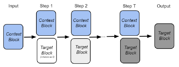
Figure 1. The overall architecture of our iterative node retrieval process. The state of the network is described by two vectors: $v_{\text{context}}$, which encodes the neighbors of a given node, and $v_{\text{target}}^{(t)}$, which encodes the target node. Each block has its own set of trainable weights: $\Psi_{\text{context}}$ and $\Phi_{\text{target}}$, which serve as memories in the Associative Memory network. At the initial moment of time, the context information is presented to the network, and the target node is masked. The Associative Memory dynamics then predict the target node after several recurrent iterations. During the iterative retrieval process, the context vector $v_{\text{context}}$ is fixed (shown as context block in the figure) for each step, while the target vector evolves with time.

3.1. Iterative Update Rule

Intuitively, our goal is to retrieve the target node from the memory with the help of the input context information and information from the previous step. The overall architecture of our retrieval process is shown in Fig. 1.

During the retrieval stage the update rule for our network is given by

(1) $$D_{\text{sim}}= f(\beta_{1}\Phi_{\text{target}}v_{\text{target}}^{(t)}+\beta_{2}\Psi_{\text{context}}v_{\text{context}})$$

(2) $$v_{\text{update}}^{(t)} =\Phi_{\text{target}}^{T}D_{\text{sim}}$$

(3) $$v_{\text{target}}^{(t+1)}= v_{\text{target}}^{(t)}+\alpha(v_{\text{update}}^{(t)}-v_{\text{target}}^{(t)})$$

where $v_{\text{context}}$ is the input context encoding, $v_{\text{target}}^{(t)}$ is the target encoding at the step $t$. At the beginning of the retrieval dynamics $v_{\text{target}}^{(0)}$ is initialized as a vector of zeros. The matrices $\Phi_{\text{target}}\in R^{K\times m}$ and $\Psi_{\text{context}}\in R^{K\times m}$ are memories stored in the network for target and context blocks, respectively. We store $K$ context memory patterns and $K$ target memory patterns, where each memory pattern is an $m$-dimensional vector. Both $\Psi_{\text{context}}$ and $\Phi_{\text{target}}$, are learnable parameters, $f$ is the softmax function, and parameters $\beta_{1}$ and $\beta_{2}$ control the temperature of the softmax. $D_{\text{sim}}$ is the similarity between the current pattern and all patterns stored in the network (considering both context block and target block), $v_{\text{update}}^{(t)}$ is the readout from the memory for the target block. $\alpha$ is the update rate for each step (it is a hyperparameter of our model). Intuitively, at every step our approach tries to retrieve the correct target information $v_{\text{target}}^{(t+1)}$ from the memory with the help of the context information $v_{\text{context}}$ as well as the target information from the previous step $v_{\text{target}}^{(t)}$. The target block state is gradually updated until it becomes stable.

Stored Memories as Energy Minima. The above network architecture is a special kind of Modern Hopfield Network (ramsauer2020hopfield, ; krotov2020large, ; krotov2021hierarchical, ). It can be shown that the network’s updating process is minimizing the following energy (Lyapunov) function

$$E=\frac{1}{2}\sum_{i=1}^{m}(v_{\text{target}})_{i}^{2}-\log\Big{[}\sum_{\mu=1}^{K}\exp\Big{(}\sum_{i=1}^{m}(\Phi_{\text{target}})_{{\mu}i}(v_{\text{target}})_{i}+\epsilon_{\mu}\Big{)}\Big{]}$$

where $(v_{\text{target}})_{i}$ is the $i$-th element in the final target vector $v_{\text{target}}$, $(\Phi_{\text{target}})_{{\mu}i}$ is the $i$-th element for the $\mu$-th target memory and $\epsilon_{\mu}=\sum_{i=1}^{m}(\Psi_{\text{context}})_{{\mu}i}(v_{\text{context}})_{i}$. Additionally, $(v_{\text{context}})_{i}$ is the $i$-th element for the input context vector, and $(\Psi_{\text{context}})_{{\mu}i}$ is the $i$-th element of the $\mu$-th context memory. The energy monotonically decreases as dynamics progresses. Eventually, the state of the network will converge to the local minimum corresponding to one of the stored memory patterns.

3.2. Training and Embedding Generation

In the training phase, we collect the encoding of the target block $v_{\text{target}}^{(T)}$ after $T$ steps of the iterative dynamics when the retrieval is stable, and then compute the cross entropy loss between this target state and the actual encoding for the target node (which is represented as a one hot encoded vector). This loss function is used for training the memory matrices $\Psi_{\text{context}}$ and $\Phi_{\text{target}}$ using the backpropagation algorithm.

In the embedding generation phase after the training is complete, the $K$-dimensional embedding for each node can be computed using the following equation

$$\text{node embedding}=\Psi_{\text{context}}v_{\text{context}}$$

where $v_{\text{context}}\in\mathbb{R}^{m}$ is the context encoding for that node, and $\Psi_{\text{context}}\in R^{K\times m}$ is the memory matrix for the context block, which has already been learned during the training phase. Intuitively, each element of the final embedding indicates a similarity score between the input context vector and specific memories stored in the Dense Associative Memory network.

3.3. Complexity Analysis

The most expensive part of our approach is the matrix multiplication $\Phi_{\text{target}}v_{\text{target}}^{(t)}$, where $\Phi_{\text{target}}\in R^{K\times m}$ and $v_{\text{target}}^{(t)}\in R^{m\times B}$ ($K$ is the number of memories, $m$ is the number of nodes and $B$ is the batch size). The complexity for this matrix multiplication is $\mathcal{O}(KBm)$. For each batch of data, we iterate $T$ steps. Thus, the time complexity per epoch is $\mathcal{O}(KTm^{2})$. Since both $K$ and $T$ are constant, the total time complexity is $\mathcal{O}(m^{2})$, which is similar to other baseline methods such as LINE (tang2015line, ) and SDNE (wang2016structural, ).

4. Empirical Evaluation

In this section we empirically evaluate the performance of our proposed network embedding model in node classification and linkage prediction downstream tasks on commonly used benchmarks.

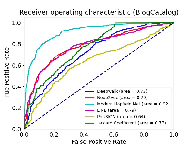
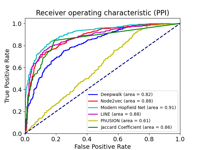
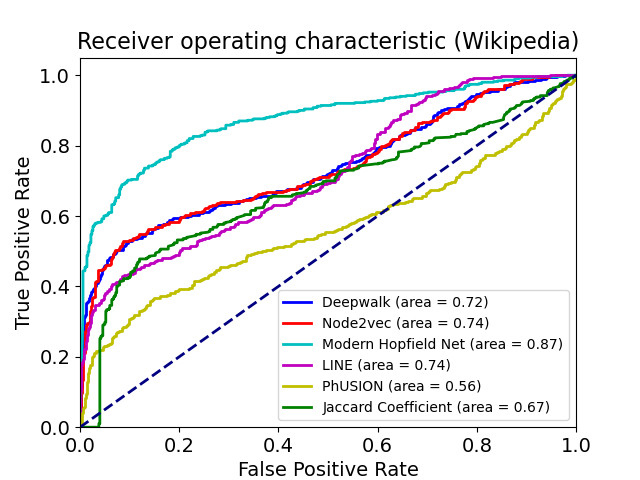
Figure 2. The Receiver operating characteristic (ROC) curve for the linkage prediction task on BlogCatalog, PPI, and Wikipedia. Comparison with popular baseline methods.

4.1. Datasets

For the network embedding generation task, we first learn unsupervised node features purely from the network’s structure and then report the performance of our embeddings for multi-label classification and linkage prediction downstream task on three datasets: BlogCatalog (reza2009social, ), Protein-Protein Interactions (oughtred2019biogrid, ) and Wikipedia (mahoney2011large, ; grover2016node2vec, ). BlogCatalog is a network of

	Blogcatalog	PPI	Wikipedia
$|V|$	10312	3890	4777
$|E|$	333983	76584	184812
categories	39	50	40

Table 1. Graph statistics for the datasets.

social relationships reflected by the blog user, and the label is indicated by the categories of the blogs. Protein-Protein Interactions is a network which indicates the interactions of proteins that are found in humans, and the label indicates the biological state. Wikipedia is a word co-occurrence network for the first $10^{9}$ bytes of the English Wikipedia dump. There exists an edge between words co-occuring in a 2-length window. The statistics of the networks and number of labels/categories for the nodes are summarized in Table 1.

Dataset	Ours	Deepwalk	Node2vec	LINE	PhUSION
Blogcatalog	$40.26^{\pm 0.53}$/$24.23^{\pm 0.97}$	$\mathbf{42.76^{\pm 1.28}}$/$\mathbf{28.48^{\pm 1.36}}$	$38.24^{\pm 1.23}$/$21.61^{\pm 1.42}$	$37.19^{\pm 1.15}$/$20.59^{\pm 1.35}$	$18.03^{\pm 0.72}$/$3.58^{\pm 0.22}$
PPI	$\mathbf{26.11^{\pm 1.48}}$/$\mathbf{21.29^{\pm 1.36}}$	$23.39^{\pm 1.29}$/$19.19^{\pm 1.51}$	$22.19^{\pm 1.78}$/$18.63^{\pm 2.09}$	$21.55^{\pm 1.56}$/$17.75^{\pm 1.88}$	$11.17^{\pm 0.14}$/$5.25^{\pm 0.71}$
Wikipedia	$\mathbf{57.62^{\pm 0.98}}$/$\mathbf{13.84^{\pm 0.73}}$	$50.56^{\pm 1.38}$/$10.19^{\pm 1.11}$	$50.13^{\pm 1.68}$/$9.73^{\pm 0.85}$	$51.21^{\pm 1.81}$/$10.31^{\pm 1.02}$	$43.82^{\pm 1.71}$/$5.51^{\pm 0.59}$

Table 2. Average micro-f1/macro-f1 scores for the multi-label classification task. We use $7$ update steps for the retrieval dynamics of our model and $2000$ hidden units for storing the memories.

Dataset	Ours	DeepWalk	Node2vec	LINE	Jaccard’s Coefficient	PhUSION
BlogCatalog	0.92$(16\%)$	0.73	0.79	0.79	0.77	0.64
PPI	0.91 $(3\%)$	0.82	0.88	0.88	0.86	0.61
Wikipedia	0.87$(17\%)$	0.74	0.74	0.72	0.67	0.56

Table 3. Area Under the Curve (AUC) scores for linkage prediction. Comparison with popular baselines. The number in parenthesis shows the performance gain when compared with the second best baseline.

4.2. Baseline Methods and Metrics

We compare our embedding approach against Deepwalk (perozzi2014deepwalk, ), LINE (tang2015line, ), Node2vec (grover2016node2vec, ), and PhUSION (zhu2021node, ), which are commonly used approaches for learning the latent node representations. Deepwalk first represents the network by a set of random walks starting from random nodes in the graph, so that a node’s neighbor information can be reflected by the neighbor information in the random walk sequence. The node embedding is obtained by embedding the random walk sequences using the SkipGram model (mikolov2013efficient, ). Node2vec is a modification of DeepWalk with a small difference in random walks. It uses two parameters to control the breadth and depth of the exploration. LINE optimizes a carefully designed objective function that preserves both local and global network structures. PhUSION proposes a unified architecture of the general embedding process, which consists of node proximity calculation, nonlinear transformation function, and embedding functions.

For the node classification downstream evaluation, we follow the procedure of previous methods, i.e. train a one-vs-rest logistic regression implemented by the LibLinear library (fan2008liblinear, ) on top of all the embedding for the classification task and report the micro-f1 and macro-f1 scores based on the average performance of 20 runs. In our experiments, the train/test split for the evaluation is $9:1$, and we also report the standard deviation. For our embedding model, we use 2000 memories across all datasets. For the baseline models we have run their codes using the default setting. All the parameters are learned by the backpropagation algorithm.

For the linkage prediction downstream evaluation, we randomly sample 500 positive and negative node pairs respectively for each dataset. The task is to predict whether or not there is connection between the node pairs based on their node embedding. The probability of an edge between nodes $i$ and $j$ is given by $\sigma(h_{i}^{T}h_{j})$, where $\sigma$ is the sigmoid function, and $h_{i},h_{j}$ are node embeddings. We report Receiver Operating Characteristic (ROC) curve as well as the Area Under Curve (AUC) scores for all the embedding methods. Also, we include a heuristic method using Jaccard’s Coefficient for reference. The Jaccard’s Coefficient is defined as $\frac{|N(u)\cap N(v)|}{|N(u)\cup N(v)|}$ for a given node pair $(u,v)$ with the immediate neighbor sets $N(u)$ and $N(v)$ respectively.

For our graph node embedding generation, Adam optimizer and weight decay is used during training, and learning rate is initialized as 0.01; $\beta_{1}$ is 1, $\beta_{2}$ is 0.5, and the update rate $\alpha$ is 0.2.

4.3. Network Embedding Empirical Evaluation

Node Classification:

Table 2 summarizes the results for graph node embeddings generated by different methods on the downstream node classification task. Our MHN based approach outperforms DeepWalk, Node2vec, LINE and PhUSION on two out of three datasets both for micro- and macro-f1 scores. On BlogCatalog our method loses to DeepWalk, but still performs better than other methods. Associative Memory network works particularly well on the Wikipedia dataset resulting in more than $7\%$ improvement over DeepWalk and Node2vec, and over $6\%$ improvement over LINE for the micro-f1 score.

Linkage Prediction:

Table 3 and Fig. 2 summarize the results for the downstream linkage prediction task. For every pair of nodes the dot product of their embedding vectors is passed through a sigmoid function and thresholded at a certain value. Scores above the threshold are predicted as links, and below the threshold as absence of links. The ROC curves are obtained as the discrimination threshold is varied. Our Associative Memory based method does extremely well on the linkage prediction task across all the benchmark datasets. Such a strong performance is expected from the conceptual computational design of our network. On the one hand, nodes with similar neighborhood structure tend to have a link connecting them. On the other hand, nodes with similar neighborhood structure will be more likely attracted (in the course of the Hopfield dynamics) by the same group of memories. Thus, the core computational strategy of our model is particularly well suited for this task.

5. Conclusions

In this work we have proposed a framework for learning node embeddings using the Modern Hopfield Networks in combination with the masked node training. The context of each node activates a set of memory vectors that are used for predicting the identity of the masked node. From the theoretical perspective, our main contribution is the extension of the Modern Hopfield Network framework to the settings where each data point (a given node in the graph) is represented by several distinct kinds of attributes (e.g. context, target node identity, labels). Some of these attributes (e.g. masked node identity) can evolve in time using the Hopfield dynamics, while others (e.g. context) can be kept clamped to guide the dynamical trajectory in the direction of appropriate (for that context) memories. The core computational strategy of the Dense Associative Memory network naturally informs the appropriate pattern completion for the masked node and learns useful representations for the memory vectors, which can be utilized for multiple downstream tasks.

Our work opens up several avenues for future work. We plan to do a more extensive comparison on a larger variety of networks, and other methods for learning unsupervised structural representations. Other directions include developing hierarchical Associative Memories to capture higher-level graph features.

References

- (1) Amit, D. J., Gutfreund, H., and Sompolinsky, H. Storing infinite numbers of patterns in a spin-glass model of neural networks. Physical Review Letters 55, 14 (1985), 1530.
- (2) Anderson Jr, W. N., and Morley, T. D. Eigenvalues of the laplacian of a graph. Linear and multilinear algebra 18, 2 (1985), 141–145.
- (3) Cao, S., Lu, W., and Xu, Q. Grarep: Learning graph representations with global structural information. In Proceedings of the 24th ACM international on conference on information and knowledge management (2015), pp. 891–900.
- (4) Demircigil, M., Heusel, J., Löwe, M., Upgang, S., and Vermet, F. On a model of associative memory with huge storage capacity. Journal of Statistical Physics 168, 2 (2017), 288–299.
- (5) Fan, R.-E., Chang, K.-W., Hsieh, C.-J., Wang, X.-R., and Lin, C.-J. Liblinear: A library for large linear classification. the Journal of machine Learning research 9 (2008), 1871–1874.
- (6) Golub, G. H., and Reinsch, C. Singular value decomposition and least squares solutions. In Linear algebra. Springer, 1971, pp. 134–151.
- (7) Grover, A., and Leskovec, J. node2vec: Scalable feature learning for networks. In Proceedings of the 22nd ACM SIGKDD international conference on Knowledge discovery and data mining (2016), pp. 855–864.
- (8) He, X., and Niyogi, P. Locality preserving projections. Advances in neural information processing systems 16, 16 (2004), 153–160.
- (9) Hertz, J. A. Introduction to the theory of neural computation. CRC Press, 2018.
- (10) Hofmann, T., and Buhmann, J. Multidimensional scaling and data clustering. Advances in neural information processing systems (1995), 459–466.
- (11) Hopfield, J. J. Neural networks and physical systems with emergent collective computational abilities. Proceedings of the national academy of sciences 79, 8 (1982), 2554–2558.
- (12) Hopfield, J. J. Neurons with graded response have collective computational properties like those of two-state neurons. Proceedings of the national academy of sciences 81, 10 (1984), 3088–3092.
- (13) Jiang, R., Fu, W., Wen, L., Hao, S., and Hong, R. Dimensionality reduction on anchorgraph with an efficient locality preserving projection. Neurocomputing 187 (2016), 109–118.
- (14) Krotov, D. Hierarchical associative memory. arXiv preprint arXiv:2107.06446 (2021).
- (15) Krotov, D., and Hopfield, J. Large associative memory problem in neurobiology and machine learning. arXiv preprint arXiv:2008.06996 (2020).
- (16) Krotov, D., and Hopfield, J. J. Dense associative memory for pattern recognition. arXiv preprint arXiv:1606.01164 (2016).
- (17) Mahoney, M. Large text compression benchmark. http://www.mattmahoney.net/dc/text.html, 2011.
- (18) Mikolov, T., Chen, K., Corrado, G., and Dean, J. Efficient estimation of word representations in vector space. arXiv preprint arXiv:1301.3781 (2013).
- (19) Mikolov, T., Sutskever, I., Chen, K., Corrado, G., and Dean, J. Distributed representations of words and phrases and their compositionality. arXiv preprint arXiv:1310.4546 (2013).
- (20) Ou, M., Cui, P., Pei, J., Zhang, Z., and Zhu, W. Asymmetric transitivity preserving graph embedding. In Proceedings of the 22nd ACM SIGKDD international conference on Knowledge discovery and data mining (2016), pp. 1105–1114.
- (21) Oughtred, R., Stark, C., Breitkreutz, B.-J., Rust, J., Boucher, L., Chang, C., Kolas, N., O’Donnell, L., Leung, G., McAdam, R., et al. The biogrid interaction database: 2019 update. Nucleic acids research 47, D1 (2019), D529–D541.
- (22) Perozzi, B., Al-Rfou, R., and Skiena, S. Deepwalk: Online learning of social representations. In Proceedings of the 20th ACM SIGKDD international conference on Knowledge discovery and data mining (2014), pp. 701–710.
- (23) Qiu, J., Dong, Y., Ma, H., Li, J., Wang, K., and Tang, J. Network embedding as matrix factorization: Unifying deepwalk, line, pte, and node2vec. In Proceedings of the eleventh ACM international conference on web search and data mining (2018), pp. 459–467.
- (24) Ramsauer, H., Schäfl, B., Lehner, J., Seidl, P., Widrich, M., Gruber, L., Holzleitner, M., Pavlović, M., Sandve, G. K., Greiff, V., et al. Hopfield networks is all you need. arXiv preprint arXiv:2008.02217 (2020).
- (25) Reza, Z., and Huan, L. Social computing data repository. http://datasets.syr.edu/pages/home.html, 2009.
- (26) Tang, J., Qu, M., and Mei, Q. Pte: Predictive text embedding through large-scale heterogeneous text networks. In Proceedings of the 21th ACM SIGKDD international conference on knowledge discovery and data mining (2015), pp. 1165–1174.
- (27) Tang, J., Qu, M., Wang, M., Zhang, M., Yan, J., and Mei, Q. Line: Large-scale information network embedding. In Proceedings of the 24th international conference on world wide web (2015), pp. 1067–1077.
- (28) Tian, F., Gao, B., Cui, Q., Chen, E., and Liu, T.-Y. Learning deep representations for graph clustering. In Proceedings of the AAAI Conference on Artificial Intelligence (2014), vol. 28.
- (29) Wang, D., Cui, P., and Zhu, W. Structural deep network embedding. In Proceedings of the 22nd ACM SIGKDD international conference on Knowledge discovery and data mining (2016), pp. 1225–1234.
- (30) Yang, C., Liu, Z., Zhao, D., Sun, M., and Chang, E. Y. Network representation learning with rich text information. In IJCAI (2015), vol. 2015, pp. 2111–2117.
- (31) Zhu, J., Lu, X., Heimann, M., and Koutra, D. Node proximity is all you need: Unified structural and positional node and graph embedding. In Proceedings of the 2021 SIAM International Conference on Data Mining (SDM) (2021), SIAM, pp. 163–171.