Dead-beat model predictive control for discrete-time linear systems

Abstract

In this paper, model predictive control (MPC) strategies are proposed for dead-beat control of linear systems with and without state and control constraints. In unconstrained MPC, deadbeat performance can be guaranteed by setting the control horizon to the system dimension, and adding an terminal equality constraint. It is proved that the unconstrained deadbeat MPC is equivalent to linear deadbeat control. The proposed constrained deadbeat MPC is designed by setting the control horizon equal to the system dimension and penalizing only the terminal cost. The recursive feasibility and deadbeat performance are proved theoretically.

1 Introduction

For discrete-time systems, deadbeat control implies that the closed-loop state is identically zero after finite time steps. The essence of deadbeat control for SISO discrete-time linear systems was discovered in [3], where existence of linear deadbeat control was proved to be equivalent to controllability. A well known design strategy for linear deadbeat control is to assign all eigenvalues to the origin. More fundamental and systematic results of linear deadbeat control can be found in [13, 6] and references therein.

Deadbeat control can be designed in optimal control framework, where the core idea is calculating the deadbeat gain from quadratic cost function with proper weighting matrices and boundary conditions. In [7], the deadbeat control was solved from singular Riccati equation, where recursive strategy was applied to solve the singular Riccati equation. Analytical solution to singular Riccati equation was provided in [8], where deadbeat control was considered as a special case. Another strategy for optimal deadbeat control is to only penalize the state cost without penalizing the control cost [1]. In [15], a direct solution is proposed for singular Riccati equation to calculated the deadbeat gain.

The deadbeat control theory has been developed maturely. Recent results on deadbeat control usually focus on engineering applications. Deadbeat control is applicable especially to systems requiring high accuracy and short transient process [11]. Deadbeat strategy is also useful in observer design, where exact zero estimation error is guaranteed, such that overall performances with estimated states can be improved [10, 9, 14]. For nonlinear systems, deadbeat control is a relatively open problem, and some results are provided in [2, 16] and references therein.

In some cases, the systems are subject to hard constraints, and bounded deadbeat control should be considered. Bounded deadbeat control problem was firstly investigated geometrically in [18], where the plant eigenvalues were required to be inside the closed unite circle to guarantee the global admissibility. Model predictive control (MPC) can be introduced to guarantee bounded deadbeat control for some specific systems, e.g., permanent-magnet synchronous motor [4], interconnected heterogenerous power converters [5], and electrical vehicle charging systems [17], etc. Currently, however, fundamental and systematic results on deadbeat MPC theory are relatively limited.

In this paper, we are proposing fundamental solutions to the deadbeat control problem in the MPC framework, such that the deadbeat performance can be achieved by bounded control with improved transient process. Main contributions of this paper include: 1) deadbeat controls are designed and proved in a systematic MPC framework; 2) implicit and explicit solutions are provided for unconstrained linear deadbeat MPC; and 3) constrained deadbeat MPC is designed for linear systems subject to state and control constrains.

2 Problem formulation

In this paper, we consider the single-input-single-output (SISO) discrete-time linear system:

$$x(k+1)=Ax(k)+Bu(k)$$ (1)

where $x\in\mathbb{R}^{n}$ and $u\in\mathbb{R}$ are the system state and control input, respectively; and $(A,B)$ is controllable.

The system is subject to state and control constraints

$$x\in\mathcal{X},~{}~{}u\in\mathcal{U},$$ (2)

where $\mathcal{X}$ and $\mathcal{U}$ are convex, and contain the origin.

The objective is to design $u(k)$ in MPC frameworks such that, for some $T>0$, it holds that $x(k)=0$ for all $k\geq T$.

3 Unconstrained dead-beat MPC

In this section, no constraints are exerted on states or control inputs, i.e., constraints (2) is not considered in this section. In the framework of unconstrained MPC, deadbeat control can be implemented through two strategies, namely deadbeat MPC with terminal equality constraint and deadbeat MPC with only terminal cost. Both strategies requires the control horizon be equal to state dimensions, namely $N=n$.

3.1 Uncosntrained deadbeat MPC with terminal equality constraint

In this deadbeat strategy, we add an extra terminal equality constraint to the original unconstrained optimization to guarantee the finite-time convergence.

Define the state sequence and control sequence at time $k$ by

$$X(k)= [x^{T}(1|k),\cdots,x^{T}(N|k)]^{T},$$

$$U(k)= [u^{T}(0|k),\cdots,u^{T}(N-1|k)]^{T},$$

where $(i|k)$ denotes the prediction $i$ steps ahead from time $k$; and $N$ is the control horizon. Throughout the paper, the prediction horizon is set equal to the control horizon.

In this deadbeat MPC, two key settings include: 1) the control horizon is set equivalent to state dimension, i.e., $N=n$; and 2) a terminal equality constraint $x(n|k)=0$ is added to the original unconstrained optimization.

The optimization is formulated by

$$U^{\ast}(k)=\mathrm{arg}\min_{U(k)}\sum_{i=1}^{n}\|x(i|k)\|^{2}_{Q}+\|u(i-1|k)\|^{2}_{R},$$ (3)

s.t. $$x(i+1|k)=Ax(i|k)+Bu(i|k),~{}~{}i=0,\cdots,n-1,$$ (4)

$$x(n|k)=0,$$ (5)

where $n$ is the dimension of $x$. The deadbeat MPC is implemented in receding horizon scheme:

$$u(k)=[1~{}0~{}\cdots~{}0]U^{\ast}(k).$$ (6)

Theorem 1

Consider the linear system (1), and suppose that no constraints are exerted. Suppose also that $(A,B)$ is completely controllable. The MPC is calculated from the optimization (3)–(5), and implemented by (6). Then,

1. the optimization (3)–(5) is feasible globally;

2. the closed-loop state satisfies $x(k)=0$ for all $k>n$.

Proof: The behavior of (1) can be predicted by

$$x(1|k)= Ax(k)+Bu(0|k),$$ (7)

$$x(2|k)= A^{2}x(k)+ABu(0|k)+Bu(1|k),$$ (8)

$$\vdots$$

$$x(n|k)= A^{n}x(k)+[A^{n-1}B~{}A^{n-2}B~{}\cdots~{}B]U(k),$$ (9)

where, since $(A,B)$ is controllable, the square matrix

$$S\triangleq[A^{n-1}B~{}A^{n-2}B~{}\cdots~{}B]$$

is invertible. It indicates that a unique control sequence $U^{\ast}(k)$ always exists, such that (5) is satisfied. Consequently, the optimization is always feasible regardless of initial states. This completes the proof of 1).

At time $k=0$, the optimal control sequence is unique, and the corresponding optimal state sequence is also unique:

$$U^{\ast}(0)= [u^{\ast}(0|0),\cdots,u^{\ast}(n-1|0)]^{T},$$

$$X^{\ast}(0)= [x^{\ast T}(1|0),\cdots,x^{\ast T}(n-1|0),0]^{T},$$

where $u(0)=u^{\ast}(0|0)$ is implemented, and $x(1)=x^{\ast}(1|0)$ can be obtained.

At time $k=1$, the optimal control sequence and the optimal state sequence are still unique, and they have to be

$$U^{\ast}(1)= [u^{\ast}(1|0),\cdots,u^{\ast}(n-1|0),0]^{T},$$

$$X^{\ast}(1)= [x^{\ast T}(2|0),\cdots,x^{\ast T}(n-1|0),0,0]^{T},$$

where $u(1)=u^{\ast}(0|1)=u^{\ast}(1|0)$ is implemented, and $x(2)=x^{\ast}(1|1)=x^{\ast}(2|0)$ can be obtained.

At time $k=n-1$, the unique control sequence and the optimal state are unique, and they have to be

$$U^{\ast}(n-1)= [u^{\ast}(n-1|0),0,\cdots,0]^{T},$$

$$X^{\ast}(n-1)= [0,\cdots,0]^{T},$$

where $u(n-1)=u^{\ast}(0|n-1)=u^{\ast}(n-1|0)$ is implemented, and $x(n)=0$. It implies that, $u(k)=0$ and $x(k)=0$ for all $k>n$. This completes the proof of 2). $\square$

It follows from the terminal equality constraint (5) and the predictive state sequence (9) that the control sequence can be solved uniquely and explicitly by

$$U(k)=-S^{-1}A^{n}x(k),$$ (10)

and the MPC can be calculated explicitly by

$$u(k)=-[1~{}0~{}\cdots~{}0]S^{-1}A^{n}x(k)=-K_{db}x(k),$$ (11)

where the deadbeat control gain is calculated by

$$K_{db}=[1~{}0~{}\cdots~{}0]S^{-1}A^{n}=S^{T}_{n}A^{n},$$ (12)

and $S_{n}^{T}$ is the first row of $S^{-1}$.

Theorem 2

If the control gain is calculated by (12), then all eigenvalues of $A-BK_{db}$ are zero, and $x(k)=0$ for all $k>n$.

Proof: For matrix $A$, there always exists invertible transformation matrix $T$, such that

$$TAT^{-1}=\begin{bmatrix}0_{(n-1)\times 1}&I_{(n-1)\times(n-1)}\\ -a_{0}&-a_{1}~{}~{}\cdots~{}~{}-a_{n-1}\end{bmatrix},~{}~{}TB=\begin{bmatrix}0_{(n-1)\times 1}\\ 1\end{bmatrix}.$$

According to linear control theory [12], the tranformation matrix $T$ is calculated by

$$T=\begin{bmatrix}S_{n}&A^{T}S_{n}&\dots&(A^{n-1})^{T}S_{n}\end{bmatrix}^{T}.$$

It then follows that

$$TBK_{db}=\begin{bmatrix}0_{(n-1)\times 1}\\ 1\end{bmatrix}[1~{}0~{}\cdots~{}0]S^{-1}A^{n}=\begin{bmatrix}0_{(n-1)\times n}\\ S_{n}^{T}A^{n}\end{bmatrix},$$

where $S_{n}^{T}$ is the first row of $S^{-1}$. In another aspect,

$$\begin{bmatrix}0_{(n-1)\times n}\\ -a_{0}~{}\cdots~{}-a_{n-1}\end{bmatrix}T= \begin{bmatrix}0_{(n-1)\times n}\\ -S_{n}^{T}\sum_{i=0}^{n-1}a_{i}A^{i}\end{bmatrix}=\begin{bmatrix}0_{(n-1)\times n}\\ S_{n}^{T}A^{n}\end{bmatrix}$$

$$= TBK_{db},$$

where Cayley-Hamilton theorem is applied. Consequently,

$$TBK_{bd}T^{-1}= \begin{bmatrix}0_{(n-1)\times n}\\ -a_{0}~{}\cdots~{}-a_{n-1}\end{bmatrix},$$

$$T(A-BK_{db})T^{-1}= \begin{bmatrix}0_{(n-1)\times 1}&I_{(n-1)\times(n-1)}\\ 0&0_{1\times(n-1)}\end{bmatrix},$$

indicating eigenvalues of $A-BK_{db}$ are all zero. As a result, it holds that $x(k)=0$ for all $k>n$. $\square$

3.2 Unconstrained dead-beat MPC with terminal cost

This deadbeat strategy is cited from [8], where the deadbeat control is solved from inverse optimization. We explain the deadbeat control in MPC framework, and extended it to the constrained case in the next section.

The optimization only penalizes the terminal cost without penalizing other stage costs. In this regard, the cost function is constructed by $J(k)=x^{T}(n|k)Px(n|k)$, and the control horizon is set to the state dimension.

The optimization is established by

$$U^{\ast}(k)=\mathrm{arg}\min_{U(k)}x^{T}(n|k)Px(n|k),$$ (13)

s.t. $$x(i+1|k)=Ax(i|k)+Bu(i|k),~{}~{}i=0,\cdots,n-1,$$ (14)

and the deadbeat MPC is implemented by (6).

Theorem 3

Consider the linear system (1), and suppose that no constraints are exerted. Suppose also that $(A,B)$ is completely controllable. The MPC is calculated from optimization (13) and implemented by (6). Then, the closed-loop state satisfies $x(k)=0$ for all $k>n$.

Proof: Without any hard constraints, the optimal terminal state minimizing $x^{T}(n|k)Px(n|k)$ is $x(n|k)=0$. Then the proof follows from that of Theorem 1. $\square$

The optimization can also be solved analytically by

$$\left.\frac{\partial\left(x^{T}(n|k)Px(n|k)\right)}{\partial U}\right|_{U=U^{\ast}}=0,$$ (15)

where $x(n|k)$ is calculated by (9). Solving (15) yields

$$2(A^{n}x(k)+SU^{\ast}(k))^{T}PS=0,$$ (16)

where $P$ and $S$ are invertible. The explicit solution to (16) is exactly the same as (10)–(12).

4 Constrained dead-beat MPC

The unconstrained deadbeat MPC with terminal cost can be extended to the constrained case. Key settings include: 1) the control horizon is set equal to the dimension of system state, i.e., $N=n$; 2) only the terminal cost is penalized, i.e., $J(k)=x^{T}(n|k)Px(n|k)$; and 3) the postive definite weighting matrix $P$ is solved from the Lyapunov equation

$$A_{K}^{T}PA_{K}-P=-Q-K^{T}RK,$$ (17)

where $Q$ and $R$ are positive definite matrices; the control gain $K$ is selected such that all eigenvalues of $A_{K}=A-BK$ are inside the unit circle.

The optimization is constructed by

$$U^{\ast}(k)=\mathrm{arg}\min_{U(k)}x^{T}(n|k)Px(n|k),$$ (18)

s.t. $$x(i+1|k)=Ax(i|k)+Bu(i|k),~{}~{}i=0,\cdots,n-1,$$ (19)

$$x(i|k)\in\mathcal{X},~{}~{}u(i-1|k)\in\mathcal{U},~{}~{}i=1,\cdots,n,$$ (20)

$$x(n|k)\in\mathcal{X}_{f},$$ (21)

where $\mathcal{X}_{f}$ denotes the terminal constraint satisfying

$$\mathcal{X}_{f}\subset\mathcal{X},$$ (22)

$$x(k)\in\mathcal{X}_{f}~{}~{}\Rightarrow~{}~{}-K_{db}x(k)\in\mathcal{U},$$ (23)

$$x(k)\in\mathcal{X}_{f}~{}~{}\Rightarrow~{}~{}(A-BK_{db})x(k)\in\mathcal{X}.$$ (24)

The MPC is impemented in receding horizon scheme (6).

Remark 1

The condition (24) indicates that $\mathcal{X}_{f}$ is an invariant set of the deadbeat closed-loop system. Here we do not have to calculate $K_{db}$ in advance to obtain the largest invariant set; instead, a sufficiently small set $\mathcal{X}_{f}$ can be chosen such that it is a subset of the largest invariant set.

Theorem 4

Consider system (1) subject to constraints (2). The MPC is calculated by the constrained optimization (18)–(21), and implemented by (6), where the terminal weighting matrix is calculated from (17). Suppose that the constrained optimization (18) is feasible initially. Then,

1. constrained optimization (18) is feasible recursively;

2. the closed-loop system is asymptotically stable;

3. there exists a finite time $T>0$, such that the state of the closed-loop system satisfies $x(k)=0$ for all $k>T$.

Proof: 1) Suppose, at time $k$, the constrained optimization is feasible, i.e. $U^{\ast}(k)$ exists such that (2) and (21) are satisfied.

At time $k+1$, at least one feasible control sequence exists:

$$u(i|k+1)=u^{\ast}(i+1|k),~{}~{}i=0,\cdots,n-1,$$

$$u(n-1|k+1)=-K_{db}x^{\ast}(n|k),$$

where $u^{\ast}(i-1|k)$ denotes the optimal control sequence at time $k$, and $x^{\ast}(i|k)$ denotes the corresponding optimal state sequence at time $k$.

It is clear that $u(i|k+1),~{}i=0,\cdots,n-1$ satisfy the constrol constraint, and $u(n-1|k+1)=-K_{db}x^{\ast}(n|k)$ satisfies the control constraint due to (23). It is also clear that $x(i|k+1),~{}i=1,\cdots,n$ satisfy the state constraint, and $x(n|k+1)=(A-BK_{db})x(n-1|k+1)=(A-BK_{db})x^{\ast}(n|k)$ satisfies the state constraint due to (24).

Consequently, at time $k+1$, the constrained optimization is feasible, provided that it is feasible at time $k$.

2) Take $J^{\ast}(k)=x^{\ast T}(n|k)Px^{\ast}(n|k)$ as the Lyapunov candidate for $x(n|k)$. It follows that

$$J^{\ast}(k+1)-J^{\ast}(k)\leq J(k+1)-J^{\ast}(k)$$

$$= x^{T}(n|k+1)Px(n|k+1)-x^{\ast T}(n|k)Px^{\ast}(n|k)$$

$$= x^{\ast T}(n|k)A_{K}^{T}PA_{K}x^{\ast}(n|k)-x^{\ast T}(n|k)Px^{\ast}(n|k)$$

$$= x^{\ast T}(n|k)\left(A_{K}^{T}PA_{K}-P\right)x^{\ast}(n|k)$$

$$= -\|x^{\ast}(n|k)\|^{2}_{Q}-\|K_{db}x^{\ast}(n|k)\|^{2}_{R},$$

where $A_{K}=A-BK$. It indicates that $x^{\ast}(n|k)\rightarrow 0$ as $k\rightarrow\infty$.

The terminal state $x^{\ast}(n|k)$ at each time $k$ satisfies

$$x^{\ast}(n|k)=A^{n}x(k)+SU^{\ast}(k),$$ (25)

where $S=[A^{n-1}B,A^{n-2}B,\cdots,B]$ is invertible. It follows from (25) that, for each $x^{\ast}(n|k)$, the constrained control sequence is unique: $U^{\ast}(k)=S^{-1}\left(x^{\ast}(n|k)-A^{n}x(k)\right)$, and the control is implemented by

$$u^{\ast}(k)= [1,0,\cdots,0]S^{-1}\left(x^{\ast}(n|k)-A^{n}x(k)\right),$$ (26)

$$= -K_{db}x(k)+S_{n}^{T}x^{\ast}(n|k),$$ (27)

where $K_{db}$ is the unconstrained deadbeat gain obtained in Section 3.1, and $S_{n}^{T}=[1,0,\cdots,0]S^{-1}$ is the first row of $S^{-1}$.

Substituting the control (27) into the original system yields

$$x(k+1)=(A-BK_{db})x(k)+BS_{n}^{T}x^{\ast}(n|k),$$ (28)

which is the closed-loop deadbeat control system perturbed by the vanishing term $BS_{n}^{T}x^{\ast}(n|k)$.

The solution to (28) is calculated by

$$x(k)=A^{k}_{db}x(0)+[A_{db}^{k-1}B,\cdots,B]\begin{bmatrix}S_{n}^{T}x^{\ast}(n|0)\\ \vdots\\ S_{n}^{T}x^{\ast}(n|k)\end{bmatrix},$$

where $A_{db}=A-BK_{db}$.

Whenever $k\geq n$, it holds that $A_{db}^{k}=0$, and

$$x(k)=[A_{db}^{n-1}B,\cdots,B]\begin{bmatrix}S_{n}^{T}x^{\ast}(n|k-n+1)\\ \vdots\\ S_{n}^{T}x^{\ast}(n|k)\end{bmatrix}.$$ (29)

Since $x^{\ast}(n|k)\rightarrow 0$ as $k\rightarrow\infty$, it follows that $x(k)\rightarrow 0$ as $k\rightarrow\infty$, i.e., the closed-loop system is asymptotically stable.

3) Based on 1) and 2), $x(k)$ converges to the origin asymptotically, indicating that it enters $\mathcal{X}_{f}$ in finite time.

Inside the invariant set $\mathcal{X}_{f}$, the state and control constraints are actually inactive, and the optimization is actually unconstrained. Consequently, the behabior of $x(k)$ follows from that of the unconstrained deadbeat MPC, and it reaches the origin in finite time and maintains zero thereafter. $\square$

5 Numerical example

The plant to be controlled is given by

$$A=\begin{bmatrix}1.1&2&0\\ 0&0.95&1\\ 0&0&1.2\end{bmatrix},~{}~{}B=\begin{bmatrix}0\\ 0.079\\ 0.1\end{bmatrix},$$

where its dimension is $n=3$.

5.1 Unconstrained deadbeat MPC

In this section, the unconstrainned deadbeat MPC can be calculated numerically by (3) and (6), where the positive weighting matrices $Q=I_{3\times 3}$ and $R=0.1$ are set; the control horizon is set to $N=n=3$; and the terminal equality constraint is assigned to $x(3|k)=0$.

The simulation results are displayed in Fig. 1, where it can be seen that system states and the control input reach the origin in $3$ steps and are maintained thereafter. To achieve deadbeat performance, the magnitude of control might be relatively large in the transient process.

Figure 1: States and control of the closed-loop system with implicit unconstrained deadbeat MPC using the terminal equality constraint: they reach the origin in $3$ steps.

The explicit deadbeat MPC gain is calculated from (12) by

$$K_{db}= [1~{}0~{}0][A^{2}B~{}AB~{}B]^{-1}A^{3}=[7.2258~{}25.1192~{}12.6558],$$

where eigenvalues of $(A-BK_{db})$ are all zero. The simulation results for the explicit deadbeat MPC closed-loop system is shown in Fig. 2, which are the same as those in Fig. 1.

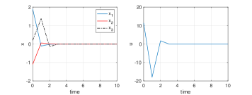
Figure 2: States and control of the closed-loop system with explicit unconstrained deadbeat MPC using the terminal equality constraint: performances are the same as those in Fig. 1 .

5.2 Constrained deadbeat MPC with terminal cost

Suppose that the control input is subject to hard constraint given by $-6\leq u\leq 6$.

In the proposed deadbeat MPC, the control horizon is set to $N=3$ which equals the system dimension. A linear feedback $K=[2.2150~{}15.0471~{}14.6128]$ is selected, such that eigenvalues of $A-BK$ are inside the unit circle. The weighting matrix can be solved from the Lyapunov equation (17) by

$$P=\begin{bmatrix}6.1590&19.4637&5.8132\\ 19.4637&96.8173&40.0964\\ 5.8132&40.0964&29.9407\end{bmatrix}.$$

Initial states are assumed to be the same as those in unconstrained cases. Closed-loop performances are illustrated by Fig. 3, where states and control input is capable of converging to zero in finite time. The control input is bounded within its constraints, and it can be seen that the control input during transient process is significantly smaller than that in the unconstrained deadbeat MPC. Due to the constrained control input, the transient process takes 5 steps, which is relatively longer than that (3 steps) of the unconstrained case.

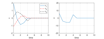
Figure 3: States and control of the closed-loop system with constrained deadbeat MPC: they converge to the origin in finite time, and the transient process is completed in 5 steps.

6 Conclusion

Deadbeat MPC strategies are proposed for SISO linear systems. The key setting is to assign the control horizon equal to the system dimension. The proposed unconstrained deadbeat MPC can be designed by either adding an terminal equality constraint or penalizing only the terminal cost. It is proved that, the unconstrained deadbeat MPC is equialvent to linear deadbeat control. The proposed constrained deadbeat MPC can be designed by penalizing only the terminal cost subject to the terminal inequality constraint. It is proved that the closed-loop state is capable of converging to the origin in finite time, while constraints are always satisfied.

References

- Emami-Naeini and Franklin [1982] Emami-Naeini, A. and Franklin, G. (1982). Deadbeat control and tracking of discrete-time systems. IEEE Transactions on Automatic Control, 27(1), 176–181.
- Haddad and Lee [2020] Haddad, W.M. and Lee, J. (2020). Finite-time stability of discrete autonomous systems. Automatica, 122, 109282.
- Kalman [1960] Kalman, R.E. (1960). On the general theory of control systems. IFAC Proceedings Volumes, 1(1), 491–502.
- Kang et al. [2019] Kang, S.W., Soh, J.H., and Kim, R.Y. (2019). Symmetrical three-vector-based model predictive control with deadbeat solution for ipmsm in rotating reference frame. IEEE Transactions on Industrial Electronics, 67(1), 159–168.
- Kreiss et al. [2021] Kreiss, J., Bodson, M., Delpoux, R., Gauthier, J.Y., Trégouët, J.F., and Lin-Shi, X. (2021). Optimal control allocation for the parallel interconnection of buck converters. Control Engineering Practice, 109, 104727.
- Kucera and Sebek [1984] Kucera, V. and Sebek, M. (1984). On deadbeat controllers. IEEE transactions on automatic control, 29(8), 719–722.
- Leden [1976] Leden, B. (1976). Dead-beat control and the riccati equation. IEEE Transactions on Automatic Control, 21(5), 791–792.
- Lewis [1981] Lewis, F. (1981). A generalized inverse solution to the discrete-time singular riccati equation. IEEE Transactions on Automatic Control, 26(2), 395–398.
- Masti et al. [2021] Masti, D., Bernardini, D., and Bemporad, A. (2021). A machine-learning approach to synthesize virtual sensors for parameter-varying systems. European Journal of Control, 61, 40–49.
- Meng [2022] Meng, D. (2022). Feedback of control on mathematics: Bettering iterative methods by observer system design. IEEE Transactions on Automatic Control, 1–1.
- Meng et al. [2022] Meng, X., Yu, H., Zhang, J., and Yan, K. (2022). Optimized control strategy based on epch and dbmp algorithms for quadruple-tank liquid level system. Journal of Process Control, 110, 121–132.
- Ogata [2010] Ogata, K. (2010). Modern control engineering. Modern control engineering.
- O’Reilly [1981] O’Reilly, J. (1981). The discrete linear time invariant time-optimal control problem—an overview. Automatica, 17(2), 363–370.
- Shang et al. [2021] Shang, C., Ding, S.X., and Ye, H. (2021). Distributionally robust fault detection design and assessment for dynamical systems. Automatica, 125, 109434.
- Sugimoto et al. [1993] Sugimoto, K., Inoue, A., and Masuda, S. (1993). A direct computation of state deadbeat feedback gains. IEEE transactions on automatic control, 38(8), 1283–1284.
- Tuna [2012] Tuna, S.E. (2012). State deadbeat control of nonlinear systems: Construction via sets. Automatica, 48(9), 2201–2206.
- Wang et al. [2019] Wang, P., Bi, Y., Gao, F., Song, T., and Zhang, Y. (2019). An improved deadbeat control method for single-phase pwm rectifiers in charging system for evs. IEEE Transactions on Vehicular Technology, 68(10), 9672–9681.
- Wing and Desoer [1963] Wing, J. and Desoer, C.A. (1963). The multiple input minimal time regulator problem (general theory). IEEE Transactions on Automatic Control, 8(2), 125–136.