An approximate diffusion process for environmental stochasticity in infectious disease transmission modelling

Abstract

Modelling the transmission dynamics of an infectious disease is a complex task. Not only it is difficult to accurately model the inherent non-stationarity and heterogeneity of transmission, but it is nearly impossible to describe, mechanistically, changes in extrinsic environmental factors including public behaviour and seasonal fluctuations. An elegant approach to capturing environmental stochasticity is to model the force of infection as a stochastic process. However, inference in this context requires solving a computationally expensive “missing data” problem, using data-augmentation techniques. We propose to model the time-varying transmission-potential as an approximate diffusion process using a path-wise series expansion of Brownian motion. This approximation replaces the “missing data” imputation step with the inference of the expansion coefficients: a simpler and computationally cheaper task. We illustrate the merit of this approach through two examples: modelling influenza using a canonical SIR model, and the modelling of COVID-19 pandemic using a multi-type SEIR model.

1 Introduction

Mathematical modelling of the complex dynamics of infectious diseases remains an essential tool to inform public health policies during epidemic outbreaks. The major focus of such modelling work is describing the intrinsic transmission dynamics and the flow of individuals between compartments that segregate the population as per their disease state. However, an epidemic is also driven by a number of extrinsic factors, including population mobility, social cycles (e.g. holidays), non-pharmaceutical interventions, and climatic variations (Bretó et al.,, 2009). In a compartmental model, such factors are often introduced explicitly through the description of the hazard (force) of infection when information about these external drivers is available (Knock et al.,, 2021; Keeling et al.,, 2020; Davies et al.,, 2020). However, while it is impossible to fully account for all extrinsic factors influencing transmission, yet ignoring this epistemic uncertainty often known as “environmental stochasticity” leads to a structural miss-specification of the model, a “model discrepancy”. Model discrepancy can lead to miss-calibrated models that underestimate uncertainty and produce biased predictions (Brynjarsdóttir and O’Hagan,, 2014). An elegant approach to account for the un-modelled model discrepancy is to represent the force of infection as a stochastic process. For example, Dureau et al., (2013); Cazelles et al., (2018) use a diffusion process for this purpose, while Birrell et al., (2021) use a discrete time stochastic process. Parameter estimation for such stochastic models is, however, challenging. Inference, particularly in a Bayesian context, requires estimation of the joint posterior distribution of both the latent path of the stochastic process and the model parameters. Estimation using a Markov chain Monte Carlo (MCMC) algorithm, involves sampling the realisation of the stochastic process, a high dimensional object, often through data-augmentation techniques, which incur a hefty computational cost (De Angelis et al.,, 2015). As a result efficient calibration of a compartmental model, which embeds a stochastic process, has received significant attention in the literature (e.g. Fuchs,, 2013; Sottinen and Särkkä,, 2008) with the goal of alleviating the computational bottleneck associated with the inference of the stochastic process.

In this paper we propose a new approach to the calibration problem through the use of a path-wise approximation of a diffusion process. Specifically, we apply a truncated Fourier expansion of a Brownian motion to obtain the approximation. Application of this series expansion turns the task of inferring a high dimensional latent diffusion sample path into the task of inferring a smaller dimensional object, the expansion coefficients, which can be carried out without data-augmentation. This method is also applicable in the context of discrete time processes that converge to a diffusion in the continuous time limit. Such processes can be approximated by first carrying out the series expansion of the limiting diffusion and then applying a suitable time discretisation. We validate the proposed method against a data augmentation technique carried out using a particle MCMC sampler proposed in Dureau et al., (2013), using a dataset from an influenza outbreak in a boarding school. We then apply this method to fit a model of COVID-19 spread in England during the first wave.

2 Background: Epidemic models with a time-varying transmission-potential

We consider the canonical SIR (Susceptible-Infected-Removed) model (Anderson et al.,, 1992) to introduce the stochastic modelling framework, although the methodology can be applied to other more complex compartmental models. In the SIR model the compartments denote the number of susceptible ($S$), infected ($I$), and recovered ($R$) people in a population subjected to an epidemic at time $t$. For a population of size $N$, the SIR model is defined by the following ODE system:

$$\frac{dS_{t}}{dt}=-\beta S_{t}\frac{I_{t}}{N},\quad\frac{dI_{t}}{dt}=\beta S_{t}\frac{I_{t}}{N}-\gamma I_{t},\quad\frac{dR_{t}}{dt}=\gamma I_{t},$$ (1)

where $\lambda=\beta\frac{I_{t}}{N}$ is the force of infection, describing the generation of infections with a transmission-potential $\beta$, between susceptible individuals and the fraction, $I_{t}/N$, of infectious individuals. The expected period spent in the compartment is given by $\gamma^{-1}$. The individual compartment sizes sum to $N=S_{t}+I_{t}+R_{t}$.

To include environmental stochasticity we introduce a time-varying $\beta_{t}$ (e.g. Ellner et al.,, 1998; Martinez-Bakker et al.,, 2015; Cauchemez and Ferguson,, 2008; Cauchemez et al.,, 2008; Cazelles and Chau,, 1997) to mitigate model discrepancy, leading to a reformulation of the model in Eq (1):

$$dx_{t} =a(x_{t},\boldsymbol{\xi})dt+b(x_{t},\boldsymbol{\xi})dW_{t}$$ (2)

$$\beta_{t} =g(x_{t})$$

$$\frac{dS_{t}}{dt} =-\beta_{t}S_{t}\frac{I_{t}}{N},\quad\frac{dI_{t}}{dt}=\beta_{t}S_{t}\frac{I_{t}}{N}-\gamma I_{t},\quad\frac{dR_{t}}{dt}=\gamma I_{t},$$

where $x_{t}$ follows a diffusion process described by an Itô stochastic differential equation (SDE) (Oksendal,, 2013) with drift $a(\cdot)$, and diffusion $b(\cdot)$ functions parameterised by the vector $\boldsymbol{\xi}$; $W_{t}$ is a standard Brownian motion; and $g(\cdot)$ is a nonlinear transformation that enforces $\beta_{t}>0$, such as exponential or inverse-logit transformation. Here we make some mild assumptions about $a(\cdot)$ and $b(\cdot)$ such as, for example, being locally Lipschitz with a linear growth bound (Oksendal,, 2013) to ensure a non-explosive solution.

Inference for the stochastic model in Eq (2) within a Bayesian framework, requires inference of the latent sample path $\boldsymbol{x}$ of the diffusion $x_{t}$, which is indirectly observed through the time evolution of the disease states: $S_{t},I_{t},R_{t}$. This is a missing data problem that can be addressed through data-augmentation based MCMC methods (e.g. Fuchs,, 2013; Dureau et al.,, 2013) in which a high resolution (in time) Euler-Maruyama discretisation of $x_{t}$ is sampled along with the model parameters. Such MCMC methods incur high computational costs and have reduced efficiency in terms of mixing and speed of convergence. In what follows we will investigate a scalable approximation of $x_{t}$ that is faster to sample.

3 Methods

Following Lyons et al., (2012); Luo, (2006); Ghosh et al., (2022), we carry out a Fourier expansion of a Brownian motion $W_{t}$ and obtain a smooth path-wise series approximation. Using this approximation of a Brownian motion, we can in turn approximate the SDE for $x_{t}$ with a random ODE. Inference of $x_{t}$ can then be carried out by inferring coefficients of this ODE, without requiring data-augmentation.

3.1 Fourier expansion of Brownian motion

Within a time interval $[0,T]$, where $T$ is the length of the time horizon within which an epidemic is analysed, the Fourier expansion of a Brownian motion $W_{t}$ is given by (Luo,, 2006):

$$W_{t}=\sum_{i=1}^{\infty}\Big{(}\int_{0}^{T}\phi_{i}(s)dW_{s}\Big{)}\int_{0}^{t}\phi_{i}(u)du.$$ (3)

where $\{\phi_{i}\}_{i=1}^{\infty}$ is a complete orthonormal basis of $L^{2}[0,T]$ (see Appendix A for derivation). For example this can be the generalised Fourier cosine basis (Lyons et al.,, 2014) given by

$$\phi_{i}(t)=(2/T)^{1/2}\cos\{(2i-1)\pi t/2T\}.$$ (4)

We will use the shorthand $Z_{i}=\int_{0}^{T}\phi_{i}(s)dW_{s}$. Since the basis functions $\{\phi_{i}\}$ are deterministic and orthonormal, it follows from standard results of Itô calculus that $Z_{i}\sim\mathcal{N}(0,1)$ (Luo,, 2006). By truncating the infinite series in Eq (27) to $n$-terms we obtain a path-wise approximation of the Brownian motion $W_{t}$ given by

$$\hat{W}_{t}=\sum_{i=1}^{n}Z_{i}\int_{0}^{t}\phi_{i}(u)du.$$ (5)

3.2 Approximating a SDE with a random ODE

Taking derivative of $\hat{W}_{t}$ with respect to time we obtain the following approximation to white noise, the derivative of Brownian motion, given by

$$\frac{d\hat{W}_{t}}{dt}=\sum_{i=1}^{n}Z_{i}\phi_{i}(t).$$ (6)

Now, let us replace the Itô SDE in Eq (2) with the following Stratonovich SDE (Oksendal,, 2013)

$$dx_{t}=a^{\prime}(x_{t},\boldsymbol{\xi})dt+b(x_{t},\boldsymbol{\xi})\circ dW_{t},$$ (7)

where $(\circ)$ denotes a Stratonovich integral (Oksendal,, 2013) with respect to $W_{t}$. The Itô SDE in Eq (2) and the Stratonovich SDE given above are equivalent (Oksendal,, 2013) if

$$a^{\prime}(x_{t},\boldsymbol{\xi})=a(x_{t},\boldsymbol{\xi})-\frac{b(x_{t},\boldsymbol{\xi})}{2}\frac{\partial b(x_{t},\boldsymbol{\xi})}{\partial x_{t}}b(x_{t},\boldsymbol{\xi}).$$ (8)

By substituting the term $dW_{t}$ in Eq (7) with the approximation $d\hat{W}_{t}$ in Eq (6), we obtain the following (random) ODE:

$$\frac{d\hat{x}_{t}}{dt}=a^{\prime}(\hat{x}_{t},\boldsymbol{\xi})+b(\hat{x}_{t},\boldsymbol{\xi})\sum_{i=1}^{n}Z_{i}\phi_{i}(t).$$ (9)

The work of Wong and Zakai, (1965) shows that as $n\rightarrow\infty$ the solution $\hat{x}_{t}$ of the above ODE will converge to the solution $x_{t}$ of the Stratonovich SDE Eq (7) which, given the choice of $a^{\prime}(\cdot)$ in Eq (8), is an equivalent representation of the Itô SDE in Eq (2). Thus, the series approximation $\hat{x}_{t}$ of the solution $x_{t}$ of an Itô SDE converges to the solution of an equivalent Stratonovich SDE.

Next, we discuss the implications of the above approximation with regards to inference.

3.3 Inference using the series approximation

Using the path-wise series approximation of a diffusion process $x_{t}$, presented in the previous sections, we can re-write the canonical SIR model in Eq (2) as a system of coupled ODEs given by

$$\frac{d\hat{x}_{t}}{dt} =a^{\prime}(\hat{x}_{t},\boldsymbol{\xi})+b(\hat{x}_{t},\boldsymbol{\xi})\sum_{i=1}^{n}Z_{i}\phi_{i}(t)$$ (10)

$$\beta_{t} =g(\hat{x})$$

$$\frac{dS_{t}}{dt} =-\beta_{t}S_{t}\frac{I_{t}}{N},\quad\frac{dI_{t}}{dt}=\beta_{t}S_{t}\frac{I_{t}}{N}-\gamma I_{t},\quad\frac{dR_{t}}{dt}=\gamma I_{t},$$

where $a^{\prime}(\cdot)$ is given by Eq (8). Note that the randomness in the above model is now encapsulated in the expansion coefficients $\boldsymbol{Z}=(Z_{1},\ldots,Z_{n})$. Inference in this model is then relegated to the inference of all the parameters: $\boldsymbol{Z},\boldsymbol{\xi},\gamma$, and the initial values: $x_{0},S_{0},I_{0},R_{0}$. We denote the vector of the parameters governing the dynamics as $\boldsymbol{\theta}=(\boldsymbol{\xi},\gamma)$. We denote the state vector evolving in continuous time by $\boldsymbol{X}_{t}=(x_{t},S_{t},I_{t},R_{t})$, and by $\boldsymbol{X}_{0}=(x_{0},S_{0},I_{0},R_{0})$ the vector of initial values.

In order to explain the inferential framework based on the series approximation, in Eq (10), we assume that the available data $\boldsymbol{y}_{t_{1:m}}=(y_{t_{1}},\ldots,y_{t_{m}})$ are the noisy observations of the state $I_{t}$ at $m$ time-points. Here we are simply considering prevalence data for the ease of exposition, however the same idea can be extended to more complex observational models where the observed data only provide partial (and often indirect) information of the states $\boldsymbol{X}_{t}$ (Birrell et al.,, 2021).

The inferential goal is to learn the posterior distribution of all the unknown quantities, given the data $\boldsymbol{y}_{t_{1:m}}$. We place priors $p(\boldsymbol{\theta})$, $p(\boldsymbol{Z})$, $p(\boldsymbol{X}_{0})$ on the parameters, expansion coefficients and the initial values. Note that, by construction, the $\boldsymbol{Z}=(Z_{1},\ldots,Z_{n})$ have an independent standard Normal prior, see Section 3.1. We then numerically solve Eq (10) to obtain a likelihood $p(\boldsymbol{y}_{t_{1:m}}|\boldsymbol{I}_{t_{1:m}},\boldsymbol{\epsilon})$, based on the noise assumption, where $\boldsymbol{I}_{t_{1:m}}$ is the numerical solution of the state $I_{t}$ evaluated at the $m$ time-points, and $\boldsymbol{\epsilon}$ are the parameters of the chosen data distribution. The posterior distribution, up to a normalisation constant, follows from the Bayes rule:

$$p(\boldsymbol{\theta},\boldsymbol{Z},\boldsymbol{X}_{0}|\boldsymbol{y}_{t_{1:m}})\propto p(\boldsymbol{y}_{t_{1:m}}|\boldsymbol{I}_{t_{1:m}},\boldsymbol{\epsilon})p(\boldsymbol{\theta})p(\boldsymbol{Z})p(\boldsymbol{X}_{0})p(\boldsymbol{\epsilon}).$$ (11)

Samples from the posterior distribution can be obtained using MCMC. The samples of the latent approximate diffusion path $\hat{\boldsymbol{x}}$ are simply the numerical solution of the ODE for $\hat{x}_{t}$ evaluated using samples of $\boldsymbol{\theta},\boldsymbol{Z},\boldsymbol{X}_{0}$ from the posterior distribution.

Note that if we had described $\beta_{t}$ using a SDE, then to sample the latent diffusion $\boldsymbol{x}$ we would have had to use data-augmentation. This involves imputing the sample path of the latent diffusion at the time-points of observations $t_{1:m}$ as well as at time-points in-between the observations using, say, the Euler-Maruyama scheme (Kloeden and Eckhard,, 1992). If one chooses $l$ time-points between $t_{m}$ and $t_{m-1}$ then the MCMC sampler would target $m(l+1)-l$ random variables (including $x_{0}$) related to the diffusion. Using the proposed approximation we have replaced the inference of $m(l+1)-l$ variables with $n$, which is a simpler inference problem if $n<m(l+1)-l$. Below we show that choosing a value of $n$ substantially smaller than $m(l+1)-l$ still renders an estimate of the posterior distribution that is a reliable approximation to the true posterior.

4 Evaluation

To evaluate the proposed approximation method we fit the model in Eq (10) to the data of an outbreak of influenza at a boarding school (Jackson et al.,, 2013) (see Fig 3 (a)), on the number of infections for a period of $T=14$ days among a population of size $N=763$. This dataset is publicly available in the R package outbreaks (Jombart et al.,, 2020). This dataset was previously used in Del Moral and Murray, (2015); Ryder et al., (2018) to fit a SIR model under assumption that the time varying transmission-potential can be modelled using an Ornstein–Uhlenbeck (OU) process. The model in Del Moral and Murray, (2015) is similar to the stochastic model introduced in Eq (2). Using the OU SDE for $x_{t}$ we can write the model in Eq (2) as:

$$dx_{t} =(\xi_{1}-\xi_{2}x_{t})dt+\xi_{3}dW_{t}$$ (12)

$$\beta_{t} =\exp(x_{t})$$

$$\frac{dS_{t}}{dt} =-\beta_{t}S_{t}\frac{I_{t}}{N},\quad\frac{dI_{t}}{dt}=\beta_{t}S_{t}\frac{I_{t}}{N}-\gamma I_{t},\quad\frac{dR_{t}}{dt}=\gamma I_{t},$$

where $\boldsymbol{\xi}=(\xi_{1},\ldots,\xi_{3})$ denotes the parameter vector of the OU SDE.

Here we specifically want to compare the outcome of inference using the true OU diffusion used above (SDE) with its series approximation (SA), leading to a model such as in Eq (10), given by

$$\frac{d\hat{x}_{t}}{dt}=(\xi_{1}-\xi_{2}x_{t})+\xi_{3}\sum_{i=1}^{n}Z_{i}\phi_{i}(t),$$ (13)

where we have chosen the generalised Fourier basis Eq (4) as the function $\phi_{i}(t)$.

For the SDE model the latent sample path $\boldsymbol{x}$, the diffusion parameters $\boldsymbol{\xi}$, initial value $x_{0}$ and the parameter $\gamma$ were also estimated together with the initial susceptibility, $s_{0}=S(t=0)/N$, assuming the initial recovered fraction $r_{0}=0$ and thus $i_{0}=1-s_{0}$. As this is count data we have specified a Poisson likelihood:

$$y_{t_{i}}|\boldsymbol{\theta},\boldsymbol{x},\boldsymbol{X}_{0}\sim\operatorname{Poisson}(I_{t_{i}}),\quad i=1,\ldots,m,$$ (14)

where in this case $\boldsymbol{X}_{0}=(x_{0},s_{0})$. For the SA model we used the inferential framework introduced in the previous section and used the Poisson likelihood as above:

$$y_{t_{i}}|\boldsymbol{\theta},\boldsymbol{Z},\boldsymbol{X}_{0}\sim\operatorname{Poisson}(I_{t_{i}}).$$ (15)

We chose a weakly-informative prior for the parameters governing the dynamics $\xi_{1},\ldots,\xi_{3},\gamma\sim\Gamma(2,2)$. For $s_{0}$ a $\operatorname{Beta}(2,1)$, since we expect the true value to be near or greater than $2/3$, and for the initial value of the diffusion we used a prior $x_{0}\sim\mathcal{N}\Big{(}\xi_{1}/\xi_{2},\big{(}\frac{\xi^{2}_{3}}{2\xi_{2}}\big{)}^{2}\Big{)}$, which is the stationary distribution of the OU diffusion.

For the SDE model, data-augmentation using a particle filter was employed to sample the ‘true’ diffusion’s path, following Dureau et al., (2013), and produce an unbiased estimate of the likelihood. Parameters $\gamma,\boldsymbol{\xi},\boldsymbol{X}_{0}$ were estimated using the Metropolis-Hastings (MH) algorithm, with an adaptive random-walk proposal based on algorithm 4 of Andrieu and Thoms, (2008). See B in S1 text for further details on this proposal mechanism. The likelihood estimate produced by the particle filter was used in the acceptance step of the MH algorithm. This particle-marginal Metropolis-Hastings (PMMH) MCMC scheme for jointly updating the latent diffusion path along with the parameters has been shown to have superior performance (Dureau et al.,, 2013) when compared to other data-augmentation approaches. For the PMMH, we used a Bootstrap particle filter (Gordon et al.,, 1995), where the particles are propagated using Euler-Maruyama discretisation, and set the number of particles to $1000$. Following Del Moral and Murray, (2015), we carried out the Euler-Maruyama iterations with a stepsize $\delta t=0.1$, leading to $l=9$ time-points between two observations.

For the SA model we used the Metropolis-Hastings algorithm with the same adaptive random-walk proposal (RWMH) used with the PMMH scheme and the Euler method to numerically solve the ODE adopting the same step-size that is used with the Euler-Maruyama scheme for the SDE.

Note that inference for the SDE model using PMMH will be substantially more computationally heavy compared to the inference for the ODE based SA model, irrespective of the value of $n$. This is due to the particle filter requiring multiple evaluation of the Euler-Maruyama scheme at each MCMC iteration. Even when parallelised, the particle filter will be bottlenecked by a weight-updating step (see Gordon et al., (1995) for details) requiring message-passing across processes. The Euler scheme for solving the ODE in Eq (13), in comparison, is evaluated once every iteration of a Metropolis-Hastings algorithm targeting the posterior distribution in Eq (11).

A crucial parameter for the proposed method is the number of basis functions $n$. If a value of $n$ produces a close match between the marginal densities of the true and approximate diffusion at the end of the analysis period $T$ then the approximation will be valid throughout the course of the epidemic. In this case $T=14$. In Fig 1 we compare the time $T$ marginal densities $p(\hat{x}_{t})|_{t=T}$ obtained by solving the ODE in Eq (13) associated with the SA, and $p(x_{t})|_{t=T}$ obtained from the original OU diffusion, both based on some trial parameters sampled from the prior. The value $n=15$ produces a close match between the marginal densities. We defer further discussion of the effect of $n$ on estimation to section 4.2.

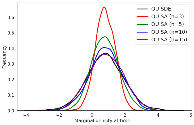
Figure 1: Comparison between the marginal density of the OU SDE at time $T=14$, with that obtained through the series approximation upon varying the number of basis $n=3,5,10,15$.

4.1 Results: comparison between true and approximate diffusion

We fitted the two models, SDE and SA respectively, using the associated algorithms as described above to the influenza dataset. We ran two chains of both PMMH, for the SDE model, and RWMH, for the SA one, for $10^{6}$ iterations where the first $5\times 10^{5}$ iterations were discarded as burnin and the remaining samples thinned to obtain $1000$ samples from the posterior distribution. The running times were $15907$ and $2397$ seconds for the PMMH and RWMH with $n=15$, respectively. We implemented a vectorised particle filter and the Euler solver for the ODE using Jax (Bradbury et al.,, 2018). The adaptive MCMC algorithm was implemented using Python.

We notice a good agreement between the parameter estimates obtained using the SDE and SA counterparts (see Fig 2). Furthermore, in Fig 3 we compare the goodness-of-fit and display the posterior distribution of the latent diffusion paths $p(\boldsymbol{x}|\boldsymbol{y}_{t_{1:m}})$ and $p(\hat{\boldsymbol{x}}|\boldsymbol{y}_{t_{1:m}})$, corresponding to the SDE and SA. Additionally, for aid of visualisation, we have also plotted draws from the (posterior) sample paths for both models in Fig 3 (c) and (d).

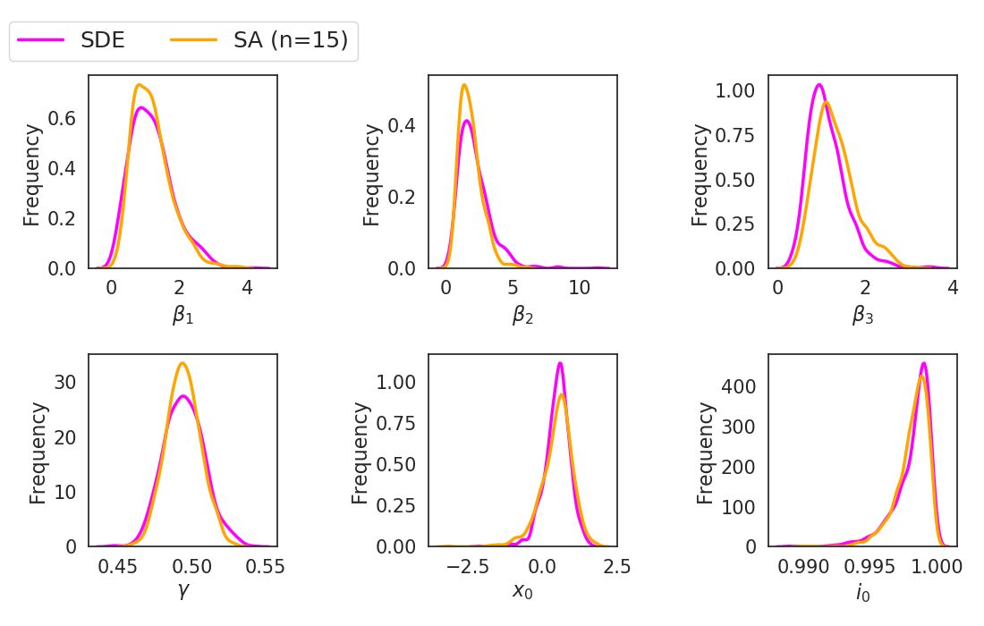
Figure 2: Comparison of the posterior marginal densities of the parameters obtained using the SDE and the SA (with $n=15$ basis function). These densities are summarised using a kernel density estimate.

We observe a good agreement between the epidemic curves obtained using the SDE and the SA, but for the posterior distribution of the latent diffusion paths the credible intervals are narrower for the SA. The SA, due to the truncation of the infinite series expansion, produces smoother paths, slightly underestimating the volatility of the latent diffusion path. On a closer introspection of the posterior means (Fig 3 (b)), it is noticeable that the latent diffusion paths drop and increase again in the period between the $4$-th and $9$-th day, around the peak, indicating sudden changes in the transmission-potential. These changes are reflected in the estimates of both SDE and SA. After the $9$-th day, the variability in the latent paths increase for both SDE and SA and the posterior means match closely. This is expected since after the peak, when the epidemic is receding, a large change in $\beta_{t}$ will have negligible effect on the case counts.

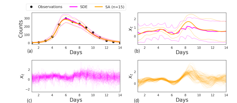
Figure 3: Influenza dataset: Goodness-of-fit (a); posterior distribution of the latent diffusion paths corresponding to the SDE and SA counterparts (b), with densities summarised by the mean (solid lines) and $95\%$ credible intervals (broken lines); and samples from the posterior distribution of the latent diffusion paths, SDE (c) and SA (d)

These results were confirmed in a simulation study where the simulated datasets mimicked this influenza dataset (see Appendix C).

4.2 Sensitivity to the choice of $n$

In Fig 1 we noticed that the marginal distribution of the latent diffusion path and its series approximation starts agreeing beyond $n\geq 10$ terms. It is worth investigating whether such a threshold exist for the posterior distributions obtained using the SDE and the SA. We did this by further comparing the joint posterior distribution $p(\boldsymbol{\theta},\boldsymbol{X}_{0}|\boldsymbol{y})$, from SDE and SA while varying $n$. Note that $\boldsymbol{\theta}$ and $\boldsymbol{X}_{0}$ are quantities which were estimated using both the SDE and SA counterparts, and thus the joint posterior of these were chosen for comparison. For this comparison we estimated the posterior distribution by fitting the SA repeatedly with number of basis set to $n=3,5,10,15,20,25,30$. To compare the posterior distributions, we used the maximum mean discrepancy (MMD) metric (Gretton et al.,, 2012), a divergence metric that can be calculated using samples from the distributions. See Appendix H for further details on this metric.

In Fig 4 we plot the MMD between the posteriors from SDE and SA for increasing $n$. For $n\geq 10$ we found good agreement between the two posteriors, consistent with the results from comparing the marginal densities (Fig 1). This reinforces our approach of choosing the number of basis by comparing marginals of the latent process, while using the SA. We summarise the runtimes of MCMC with the RWMH proposal for each choice of $n$ in Table 1, noting that the increase in the runtimes as we varied $n$ was negligible, especially when compared to the PMMH with SDE.

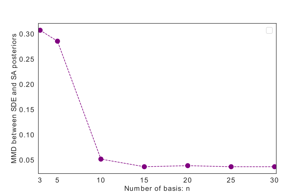
Figure 4: MMD between the joint posterior distributions of the parameters $\boldsymbol{\theta}$ and initial values $\boldsymbol{X}_{0}$ from SDE and SA (for different $n$).

Table 1: Runtimes (rounded to nearest integer), in seconds, of MCMC for SA, as a function of the number of basis $n$, in comparison with the runtime of SDE. These were run on a $3.6$ GHz machine with $16$ GB memory.

Runtimes in seconds
SA with	$n=3$	$n=5$	$n=10$	$n=15$	$n=20$	$n=25$	$n=30$	SDE
	$2280$	$2282$	$2337$	$2397$	$2470$	$2538$	$2637$	$15907$

5 Application: modelling COVID-19 outbreak in England

Our proposed method of modelling the time-varying transmission-potential as an approximate diffusion can also be applied to a discrete time stochastic process that converges to a diffusion in the continuous time limit. For example, an AR$(1)$ process converges to a OU diffusion. Thus, if one is already using an AR$(1)$ process to model the transmission-potential, then a discretised version of the series approximation of OU diffusion, the ODE in Eq (13), can be chosen as its replacement.

To exemplify the application of the series expansion method in replacing a discrete time stochastic process, we have chosen to fit a compartmental model whose dynamics are described as a set of first order difference equations, to data from the first wave of the COVID-19 outbreak in England, between February and August 2020 (Birrell et al.,, 2021). This model captures the effect of unknown extrinsic factors on the force of infection through a time-varying transmission-potential modelled as a Gaussian random-walk. We introduce the model of Birrell et al., (2021) in what follows and introduce an alternative formulation using the series approximation of Brownian motion.

5.1 Transmission model for COVID-19

This is an age and spatially structured transmission model, stratifying the population into $n_{A}=7$ age groups and $n_{r}=7$ regions. Within each region, the transmission dynamics are governed by a system of first order difference equations:

$$S_{r,t_{k},a} =S_{r,t_{k-1},a}\left(1-\lambda_{r,t_{k-1},a}\delta t\right)$$ (16)

$$E^{1}_{r,t_{k},a} =E^{1}_{r,t_{k-1},a}\left(1-\frac{2\delta t}{d_{L}}\right)+S_{r,t_{k-1},a}\lambda_{r,t_{k-1},a}\delta t$$

$$E^{2}_{r,t_{k},a} =E^{2}_{r,t_{k-1},a}\left(1-\frac{2\delta t}{d_{L}}\right)+E^{1}_{r,t_{k-1},a}\frac{2\delta t}{d_{L}}$$

$$I^{1}_{r,t_{k},a} =I^{1}_{r,t_{k-1},a}\left(1-\frac{2\delta t}{d_{I}}\right)+E^{2}_{r,t_{k-1},a}\frac{2\delta t}{d_{L}}$$

$$I^{2}_{r,t_{k},a} =I^{2}_{r,t_{k-1},a}\left(1-\frac{2\delta t}{d_{I}}\right)+I^{1}_{r,t_{k-1},a}\frac{2\delta t}{d_{I}}$$

where: $S_{r,t_{k},a}$, $E^{d}_{r,t_{k},a}$, $I^{d}_{r,t_{k},a},d=1,2$ represent the time $t_{k},k=1,\ldots,K,$ partitioning of the population of individuals in a region $r,r=1,\ldots,n_{r}$, in age-group $a,a=1,\ldots,n_{A}$, into $S$ (susceptible), $E$ (exposed) and $I$ (infectious) disease states. The average period spent in the exposed and infectious states are given by the parameters $d_{L}$ and $d_{I}$ respectively; and $\lambda_{r,t_{k},i}$ is the time- and age-varying rate with which susceptible individuals become infected, the force of infection. Time steps of $\delta t=0.5$ days are chosen to be sufficiently small relative to the latent and infectious periods. Following Birrell et al., (2011) the initial conditions of the system states $S,E^{1},E^{2},I^{1},I^{2}$ at $t_{0}$ are given by region-specific parameters $\psi_{r}$ and $I_{0,r}$, describing the initial exponential growth and the initial number of infectious individuals, respectively. New infections are generated as

$$\Delta^{\textrm{infec}}_{r,t_{k},a}=S_{r,t_{k},a}\lambda_{r,t_{k},a}\delta t,$$ (17)

where $\lambda_{r,t_{k},a}\delta t$ is driven over time by a region-specific time-varying potential, $\beta_{t_{k},r}$, which moderates the rate at which effective contact take place. This region-specific transmission-potential captures the discrepancy between how actual contact take place between the age groups, and that encoded by a set of time-varying contact matrices. We refer the reader to Birrell et al., (2021) for further details on the model dynamics and parameterisation.

Over time $\beta_{t_{k},r}$ is not allowed to vary unconstrained and a smoothing is imposed by assuming, a priori that its evolution follows a Gaussian random-walk process with volatility $\sigma_{\beta_{t}}$:

$$\log\left(\beta_{t_{k},r}\right) \sim\mathcal{N}\left(\log\left(\beta_{t_{k-1},r}\right),\sigma_{\beta_{t}}^{2}\right),\quad\text{if $t_{k}>t_{\textrm{lock}}$},$$ (18)

$$\log\left(\beta_{t_{k},r}\right) =0,\quad\text{if $t_{k}\leq t_{\textrm{lock}}$},$$

where $t_{\textrm{lock}}$ indicates the time-point corresponding to the lockdown introduced in England on ${23}^{\textrm{rd}}$ March $2020$. This random-walk formulation requires the inference of the high-dimensional (due to the choice of $\delta t$) sample path of this process, an extremely challenging task using MCMC. We will discuss this inferential difficulty later in Section 5.2.2. To restrict the dimensionality of the process, in Birrell et al., (2021) this transmission-potential is assumed to be piecewise constant with weekly changepoints, and its values at these changepoints modelled as a random-walk. Denote $w_{k}\equiv w(t_{k})$ the week in which time $t_{k}$ falls. Then the time evolution of the transmission-potential is modelled at a slower weekly time-scale:

$$\log\left(\beta_{w_{k},r}\right) \sim\mathcal{N}\left(\log\left(\beta_{w_{k-1},r}\right),\sigma_{\beta_{w}}^{2}\right),\quad\text{if $t_{k}>t_{\textrm{lock}}+7/\delta t$},$$ (19)

$$\log\left(\beta_{w_{k},r}\right) =0,\quad\text{if $t_{k}\leq t_{\textrm{lock}}+7/\delta t$},$$

$$\beta_{t_{k},r} =\beta_{w_{k},r},$$

as a Gaussian random-walk, with volatility $\sigma_{\beta_{w}}$, following the first week of the lockdown. Realisation of the process, for each region, can then be obtained by sampling the vector $\Delta\boldsymbol{\beta}_{r}$ of all the weekly increments $\Delta\beta_{w_{k},r}=\log\left(\beta_{w_{k},r}\right)-\log\left(\beta_{w_{k-1},r}\right)$. It was assumed in Birrell et al., (2021) that the contact matrices sufficiently described how actual contacts took place between different age groups prior to the lockdown and thus $\beta_{w_{k},r}=1$ over that period.

5.2 Inference

To fit the model, using a Bayesian framework, surveillance data of age- and region-specific counts of deaths in people with a lab-confirmed COVID-19 diagnosis between ${17}^{\textrm{st}}$ February and ${1}^{\textrm{st}}$ August was used. Furthermore, serological data from NHS Blood and Transplant (NHSBT), informing the fraction of the population carrying COVID-19 antibodies, were also used.

Following Birrell et al., (2021) the number of observed deaths $y^{d}_{r,t_{k},a}$ on day $t_{k}$, in age group $a$, and in region $r$ follows a negative binomial distribution:

$$y^{d}_{r,t_{k},a}|d_{I},p_{a},\psi_{r},I_{0_{r}},\Delta\boldsymbol{\beta}_{r},\eta\sim\textrm{NegBin}\left(\mu_{r,t_{k},a},\eta\right),$$ (20)

where the mean $\mu_{r,t_{k},a}=p_{a}\sum_{l=0}^{k}f_{k-l}\Delta^{\textrm{infec}}_{r,t_{l},a}$ is derived using Eq (17), an assumed-known distribution of the time from infection to death from COVID-19, $f$, and an age-specific infection-fatality ratio $p_{a}$. Here $\eta$ is a dispersion parameter such that $\mathbb{E}y^{d}_{r,t_{k},a}=\mu_{r,t_{k},a}$ and $\textrm{Var}\left(y^{d}_{r,t_{k},a}\right)=\mu_{r,t_{k},a}\left(1+\eta\right)$.

If, on day $t_{k}$, $n_{r,t_{k},a}$ blood samples are taken from individuals in region $r$ and age-group $a$, and the observed number of positive tests is $y^{s}_{r,t_{k},a}$, then

$$y^{s}_{r,t_{k},a}|d_{I},\psi_{r},I_{0_{r}},\Delta\boldsymbol{\beta}_{r},k_{\textrm{sens}},k_{\textrm{spec}}\sim\textrm{Bin}\left(n_{r,t_{k},a},k_{\textrm{sens}}\left(1-\frac{S_{r,t_{k},a}}{N_{r,a}}\right)+\left(1-k_{\textrm{spec}}\right)\frac{S_{r,t_{k},a}}{N_{r,a}}\right),$$ (21)

where $k_{\textrm{sens}}$ and $k_{\textrm{spec}}$ parametrises the sensitivity and the specificity of the serological testing process, and $S_{r,t_{k},a}$ is obtained by solving the difference equations in Eq (16). $N_{r,a}$ is the total population in age-group $a$ and region $r$.

The unknown quantities that need to be inferred can be divided into two groups: (i) Global parameters $\boldsymbol{\theta}_{g}=(\eta,d_{I},p_{1},\ldots,p_{n_{A}},k_{\textrm{sens}},k_{\textrm{spec}},\sigma_{\beta_{w}})$ shared between regions, and (ii) regional parameters specific to each region: $\boldsymbol{\theta}_{r}=(\psi_{r},I_{0_{r}},\Delta\boldsymbol{\beta}_{r})$. After placing the same priors as was used in Birrell et al., (2021) (and listed in Appendix E), the posterior distribution of the unknown quantities is as follows:

$$p(\boldsymbol{\theta}_{g},\boldsymbol{\theta}_{1},\ldots,\boldsymbol{\theta}_{n_{r}}|\boldsymbol{y^{d}},\boldsymbol{y^{s}})\propto p(\boldsymbol{\theta}_{g})\prod_{k=1}^{K}\prod_{a=1}^{n_{A}}\prod_{r=1}^{n_{r}}p(y^{d}_{r,t_{k},a}|\boldsymbol{\theta}_{g},\boldsymbol{\theta}_{r})p(y^{s}_{r,t_{k},a}|\boldsymbol{\theta}_{g},\boldsymbol{\theta}_{r})p(\boldsymbol{\theta}_{r}),$$ (22)

where we denote by $\boldsymbol{y^{d}},\boldsymbol{y^{s}}\in\mathbb{R}^{K\times{n_{A}}\times n_{r}}$ the data for all time-points, ages and regions corresponding to deaths and sero-positive tests, respectively.

5.2.1 Sampling from the posterior

Sampling from the posterior distribution Eq (22) is challenging due to the large number of random-walk increments corresponding to all regions and weeks since lockdown. MCMC with a vanilla RWMH proposal, as applied in Birrell et al., (2021), due to the linear scaling of convergence time with increasing dimensions mixes poorly and requires a large number of iterations ($\approx 10^{7}$) of the Markov chain before convergence is reached. To improve convergence we instead used a random-scan Metropolis-within-Gibbs (MwG) algorithm that circumvent the updating of a large parameter vector at each iteration. This MwG algorithm exploits the independence between the regional parameters. Our proposed sampling strategy consists of sampling alternatively, at each MCMC iteration, from the posterior of the global parameters conditioned on all the regional ones: (i) $p(\boldsymbol{\theta}_{g}|\boldsymbol{\theta}_{1},\ldots,\boldsymbol{\theta}_{n_{r}},\boldsymbol{y^{d}},\boldsymbol{y^{s}})$, and regional parameters for one randomly chosen region conditioned on the global ones (since the regional parameters are conditionally independent of any other region’s parameters): (ii) $p(\boldsymbol{\theta}_{r^{*}}|\boldsymbol{\theta}_{g},\boldsymbol{y^{d}},\boldsymbol{y^{s}})$, where $r^{*}\sim\operatorname{Uniform}(1,n_{r})$. Samples from each of these conditional distributions are obtained using an adaptive RWMH move with the same adaptation mechanism used in Section 4.1. The pseudocode for this MwG algorithm is furnished in Appendix F.

5.2.2 An alternative formulation

The number of region-specific random-walk increments $\Delta\beta_{w_{k},r}$ that needs to be sampled increases with time. The performance of the MwG algorithm starts deteriorating and exhibiting poor mixing and slow convergence, as this number becomes large. This limits dramatically the usefulness of this model in the context of a real-time application.

For the model in Eq (19), this problem can be tackled by increasing the time between two successive changepoints thus reducinge the number of increments to be sampled for a period of analysis. This is however driven by computational convenience, and it would be more meaningful to learn these changes from data. We could model the time evolution of the transmission-potential at a faster time-scale, for example as in Eq (18). However, in this case the number of random-walk increments, to be sampled per region, equals the number of time-points between lockdown and the end of analysis date. Any MCMC sampler, that uses a RWMH proposal, would struggle severely to move efficiently in such a high-dimensional parameter space.

To alleviate these problems we propose to model the transmission-potential as a Brownian motion $W_{t,r}$ with volatility $\sigma_{\beta_{t}}$ evolving in continuous time $t$ and apply the series approximation as follows:

$$\beta_{t,r} =\sigma_{\beta_{t}}\sum_{i=1}^{n}Z_{i}\int_{0}^{t}\phi_{i}(u)du$$ (23)

$$=\sigma_{\beta_{t}}\sum_{i=1}^{n}Z_{i}(2/T)^{1/2}\sin\{(2i-1)\pi t/2T\}\approx W_{t},$$

where the second equality follows from choosing $\phi_{i}$ as given in Eq (4) and carrying out the integration. We can then discretise this approximation using the same time-step of $\delta t$ that is used for the compartmental dynamics to obtain the following path-wise (discrete time) approximation:

$$\beta_{t_{k},r}=\sigma_{\beta_{t}}\sum_{i=1}^{n}Z_{i,r}(2/T)^{1/2}\sin\{(2i-1)\pi t_{k}/2T\},$$ (24)

where $T$ is the number of days between lockdown and analysis date. Note that in this formulation the problem of sampling a large vector of increments $\Delta\boldsymbol{\beta}_{r}$ is reduced to that of sampling a $n$-dimensional vector of the coefficients $\boldsymbol{Z}_{r}=(Z_{1,r},\ldots,Z_{n,r})$. From the comparison of the time $T$ marginal distributions of the true and approximate Brownian motion, as for the OU process (see Fig 1), we found $n=10$ to produce a good path-wise approximation. Thus, we used $n=10$ for the subsequent comparative evaluations. The regional parameter vector, $\boldsymbol{\theta}_{r}=(\psi_{r},I_{0_{r}},\boldsymbol{Z}_{r})$, now contains the expansion coefficients instead of the random-walk increments $\Delta\boldsymbol{\beta}_{r}$.

5.3 Results: comparative evaluations

We ran the MwG algorithm to target the posterior distribution in Eq (22) while using the random-walk based piecewise constant transmission-potential in Eq (19) and the Brownian motion approximation (BMA) in Eq (24). In both cases we ran $3\times 10^{6}$ iterations, discarded the first half of the iterations as burn-in and subsequently thinned the remaining samples to obtain $1000$ samples. We implemented the epidemic model in C++. The MwG algorithm was implemented using Python.

Fig 5 (a) compares, for the two alternative choices of modelling the transmission-potential, the posterior predictive distributions of the death data aggregated across all ages and regions with the observed data (see Appendix G in for region-specific plots). Clearly the goodness-of-fit is indistinguishable between the two models. In Fig 5 (b) we show summaries of the posterior distributions of the latent infections $p(\boldsymbol{\Delta^{\textrm{infec}}}|\boldsymbol{y^{d}},\boldsymbol{y^{s}})$, aggregated across all ages and regions (region-wise infections are shown in Appendix G) again showing close consistency across models, with the exception of a few days immediately following the lockdown where the number of infections estimated by the BMA is slightly higher.

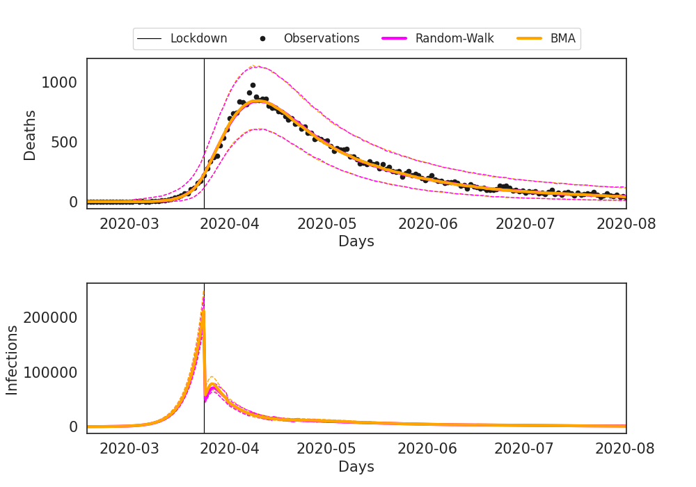
Figure 5: Goodness-of-fit of daily death data (a) and the inferred latent infections (b), produced using the random-walk (magenta lines) and BMA (orange lines). These densities are summarised by the mean (solid lines) and $95\%$ credible intervals (broken lines). The black line indicates the day of lockdown in England ${23}^{\textrm{rd}}$ March, 2020.

Following Birrell et al., (2021), we also obtain estimates of the effective region-specific reproduction number $R_{t_{k},r}$, their weighted average $R_{t,E}$ representing the reproduction number for all of England, (formulae for these are given in Appendix D in S1 text). In Fig 6 we show the posterior distributions for $p(R_{t,E}|\boldsymbol{y^{d}},\boldsymbol{y^{s}})$, using the two alternative models. It is evident that the estimate obtained from the BMA appears to be smoother than what is obtained using the piecewise constant model, more realistically reflecting the actual transmission process that happens in continuous time. In Table 2 we present infection-fatality ratio estimates from the two models, again showing close agreement across models.

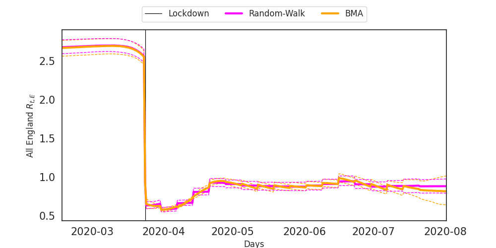
Figure 6: Posterior mean (solid lines) and $95\%$ credible intervals (broken lines) for the all England reproduction number $R_{t,E}$.

Table 2: Posterior mean and $95\%$ credible intervals for the age-specific infection-fatality ratio from the random-walk and BMA models of transmission-potential.

Age group (yrs)	Random-walk	BMA
$<5$	0.0009%	0.0009%
	(0.0002%–0.0022%)	(0.00007%–0.0019%)
5–14	0.0014%	0.0014%
	(0.0008%–0.0022%)	(0.0006%–0.0022%)
15–24	0.0046%	0.0044%
	(0.0032%–0.0062%)	(0.0029%–0.0060%)
25–44	0.0311%	0.0299%
	(0.0281%–0.0345%)	(0.0257%–0.0341%)
45–64	0.4653%	0.4488%
	(0.4412%–0.4901%)	(0.4001%–0.4976%)
65–74	3.0992%	2.9831%
	(2.9576%–3.2600%)	(2.6609%–3.3052%)
$>74$	17.8161%	17.1086%
	(16.9632%–18.6098%)	(15.3604%–18.8568%)

Computational gains:

The MwG algorithm took around $78$ hours to finish for both models of the transmission-potential. However, the BMA allows inference at a faster time-scale producing a smoother estimate of $R_{t,E}$ avoiding artificial model assumptions. Such an inference would be computationally infeasible if using a random-walk model at the more granular time-scale as in Eq (18), given the poor scaling of the RWMH proposal in high dimensions. Thus, using the series approximation we were able to extract more information about the transmission-potential and reproduction-ratio in comparison to the piecewise constant model, while incurring the same computational expense.

Had we used the random-walk model in Eq (18), we would have had to further partition each of the regional parameter block in separate chunks to accommodate a large vector of increments $\Delta\beta_{t_{k},r}=\log\left(\beta_{t_{k},r}\right)-\log\left(\beta_{t_{k-1},r}\right)$. Consequently, multiple Gibbs moves would have been necessary to update all the increments for a randomly chosen region. This, in turn, would have increased the number of likelihood computations, involving the computationally expensive updates of the transmission model, exponentially at each MCMC iteration.

6 Discussion

By modelling the force of infection as the function of a time-varying transmission-potential we can incorporate extrinsic, un-modelled effects in the description of the transmission process within a compartmental model. Describing this transmission-potential, in turn, as a stochastic process, a diffusion in particular, we can inject environmental stochasticity in an otherwise deterministic model. In this paper we proposed a path-wise approximation of a diffusion process as an alternative to modelling the dynamics of the transmission-potential as a SDE. Through the path-wise approximation we arrive at a random ODE approximating the SDE. As a function of its parameters, the path (solution) of an ODE is completely deterministic. As a result inference of the transmission-potential is simplified, with no need to solve a missing data problem using a computationally expensive data-augmentation procedure.

We demonstrate the efficacy of the proposed path-wise approximation using two epidemic models. In the first one, an influenza model, we replaced an OU SDE with an equivalent path-wise approximation. We noticed similar inference outcomes in terms of parameter estimates and goodness-of-fit using the SDE and its ODE approximation. However, for the latter we observed orders-of-magnitude improvement in computational efficiency.

We then applied the path-wise approximation to replace a Gaussian random-walk with a discretised path-wise approximation of Brownian motion to model the transmission-potential within a compartmental model of COVID-19 pandemic spread in England. Again we noticed consistent estimates of crucial unknown quantities such as infection-fatality rate, latent infections and a time-varying estimate of the reproduction number. In addition, the path-wise approximation allows the transmission-potential to be modelled at a more granular time-scale providing a smooth estimate of the effective reproduction number. This would be impossible to achieve using the random-walk model due to an exorbitant computational burden.

As an alternative to using our path-wise approximation of Brownian motion to model the transmission-potential, at a faster time-scale, we could have used a different MCMC algorithm, such as the No-U-Turn sampler (Hoffman and Gelman,, 2014), that is known to perform well for high dimensional problems. This algorithm proposes a move based on the gradient of the target density. Evaluating gradients, however, for the COVID-19 model is challenging as this requires, in addition to extra computations, a complete re-implementation of the model using an automatic differentiation package. However, for modelling studies where such re-implementation is straightforward, we like to point out that by applying a path-wise approximation of a diffusion process we are left with the task of sampling from a posterior distribution with a standard Gaussian prior (over the coefficients). The No-U-Turn sampler generally excels at this task.

In this paper we have used simple diffusion models whose transition densities are known analytically. However, if additional prior information about the force of infection is available, then such information can be incorporated in more complex nonlinear SDEs as models of the time-varying transmission-potential. Our methodology can be seamlessly applied in such cases to arrive at a path-wise approximation of such complex diffusion processes.

7 Software

Code and data supporting the experiment with the SIR model in Section 4, and the code for running the COVID-19 model in Section 5 is available at https://github.com/sg5g10/envstoch. Requests to access the non-publicly available data used for the COVID-19 model in section 5, are handled by the UKHSA Office for Data Release (ODR) https://www.gov.uk/government/publications/accessing-ukhsa-protected-data

Appendix A: Fourier expansion of Brownian motion

By the definition of an Itô integral, within a time interval $[0,T]$ a standard Brownian motion can be written as (Luo,, 2006; Lyons et al.,, 2012):

$$W_{t}=\int_{0}^{t}dW_{s}=\int_{0}^{T}\mathbb{I}_{[0,t]}(s)dW_{s},$$ (25)

where $\mathbb{I}_{[0,t]}(\cdot)$ is the indicator function. Suppose $\{\phi_{i}\}_{i=1}^{\infty}$ is a complete orthonormal basis of $L^{2}[0,T]$. We can interpret $\mathbb{I}_{[0,t]}$ as an element of $L^{2}[0,T]$, and expand it in terms of the basis functions:

$$\mathbb{I}_{[0,t]}(s) =\sum_{i=1}^{\infty}\left\langle\mathbb{I}_{[0,t]}(\cdot),\phi_{i}(\cdot)\right\rangle\phi_{i}(s)$$ (26)

$$=\sum_{i=1}^{\infty}\Big{(}\int_{0}^{t}\phi_{i}(u)du\Big{)}\phi_{i}(s).$$

Substituting (26) into (25) we see that:

$$W_{t}=\sum_{i=1}^{\infty}\Big{(}\int_{0}^{T}\phi_{i}(s)dW_{s}\Big{)}\int_{0}^{t}\phi_{i}(u)du.$$ (27)

Appendix B: Adaptive MCMC

In an adaptive MCMC algorithm optimal values of the proposal density is learnt on the fly using past samples from the Markov chain. Different mechanisms can be used to adapt or learn the parameters of the proposal. (Andrieu and Thoms,, 2008) proposed a general framework for constructing adaptive MCMC algorithms that rely on the stochastic approximation method (Robbins and Monro,, 1951) for learning the proposal’s parameters on the fly.

Consider in general the proposal density $q_{\phi}(\boldsymbol{\theta}^{j+1}|\boldsymbol{\theta}^{j})$ parameterised by $\phi$. Let us also define a suitable objective function

$$h(\phi):=\mathbb{E}^{\phi}\big{[}H(\phi,\boldsymbol{\theta}^{0},\boldsymbol{\theta}^{1},\ldots,\boldsymbol{\theta}^{j},\boldsymbol{\theta}^{j+1})\big{]},$$ (28)

that expresses some measure of the statistical performance of the Markov chain in its stationary regime. The expectation is with respect to a $\phi$ dependent distribution. For example, the coerced acceptance probability is often used as the objective:

$$H(\phi,\boldsymbol{\theta}^{0},\boldsymbol{\theta}^{1},\ldots,\boldsymbol{\theta}^{j},\boldsymbol{\theta}^{j+1})=\underbrace{\mathrm{min}\left\{1,\frac{\pi(\boldsymbol{\theta}^{j+1})}{\pi(\boldsymbol{\theta}^{j})}\frac{q_{\phi}(\boldsymbol{\theta}^{j}|\boldsymbol{\theta}^{j+1})}{q{\phi}(\boldsymbol{\theta}^{j+1}|\boldsymbol{\theta}^{j})}\right\}}_{=:\alpha^{j}}-\bar{\alpha},$$ (29)

where $\pi(\boldsymbol{\theta})$ is the target distribution and $\bar{\alpha}$ is the approximate optimal expected acceptance probability in the stationary regime. For the Gaussian proposal $q:=\mathcal{N}(\boldsymbol{\theta}^{j+1}|\boldsymbol{\theta}^{j},\boldsymbol{\Sigma}^{j})$, with its parameter $\phi$ being the covariance $\boldsymbol{\Sigma}^{j}$, the following objective function:

$$H(\boldsymbol{\Sigma}^{j},\boldsymbol{\theta}^{j+1})=\boldsymbol{\theta}^{j+1}\boldsymbol{\theta}^{{j+1}^{{}^{\prime}}}-\boldsymbol{\Sigma}^{j},$$ (30)

corresponds to matching the moments of the proposal with that of the target. Here by $a^{{}^{\prime}}$ we denote the transpose of the vector $a$.

Optimal exploration of $\pi(\boldsymbol{\theta})$ can thus be formulated as finding the root $\bar{\phi}$ of the following equation: $h(\phi)=0$. The challenge here is to devise an algorithm to find the roots of $h(\phi)$, which involves both integration and optimisation. Andrieu and Thoms, (2008) suggested using the stochastic approximation method (Robbins and Monro,, 1951) which is tailored to this situation:

$$\phi^{j+1} =\phi^{j}+\delta^{j}H(\phi^{j},\boldsymbol{\theta}^{0},\boldsymbol{\theta}^{1},\ldots,\boldsymbol{\theta}^{j},\boldsymbol{\theta}^{j+1})$$ (31)

$$=\phi^{j}+\delta^{j+1}h(\phi)+\delta^{j+1}H(\phi^{j},\boldsymbol{\theta}^{0},\boldsymbol{\theta}^{1},\ldots,\boldsymbol{\theta}^{j},\boldsymbol{\theta}^{j+1})-\delta^{j+1}h(\phi)$$

$$=\phi^{j}+\delta^{j+1}h(\phi)+\delta^{j+1}\xi^{j+1},$$

where $\xi^{j+1}:=\big{[}H(\phi^{j},\boldsymbol{\theta}^{0},\boldsymbol{\theta}^{1},\ldots,\boldsymbol{\theta}^{j},\boldsymbol{\theta}^{j+1})-h(\phi)\big{]}$ is usually referred to as the noise term and $\delta^{j}$ is a decreasing sequence (a step-size parameter). If the noise term $\xi^{j+1}$ averages to zero as $j\rightarrow\infty$, the above recursion will converge to the root $\bar{\phi}$ (or at least oscillate around it) when the following conditions hold:

$$\sum_{j=0}^{\infty}\delta^{j}=\infty\quad\operatorname{and}\quad\sum_{j=0}^{\infty}(\delta^{j})^{2}<\infty.$$ (32)

Combining the above objective functions and using the stochastic approximation we have the following recursions for adapting a random-walk proposal with a global scaling $\lambda^{j}$, $\mathcal{N}(\boldsymbol{\theta}^{j+1}|\boldsymbol{\theta}^{j},\lambda^{j}\boldsymbol{\Sigma}^{j})$, as (Andrieu and Thoms,, 2008):

$$\log(\lambda^{j+1}) =\log(\lambda^{j})+\delta^{j+1}(\alpha^{j+1}-\bar{\alpha})$$ (33)

$$\boldsymbol{\mu}^{j+1} =\boldsymbol{\mu}^{j}+\delta^{j+1}(\boldsymbol{\theta}^{j+1}-\mu^{j})$$

$$\boldsymbol{\Sigma}^{j+1} =\boldsymbol{\Sigma}^{j}+\delta^{j+1}(\boldsymbol{\theta}^{j+1}\boldsymbol{\theta}^{{j+1}^{{}^{\prime}}}-\boldsymbol{\Sigma}^{j}),$$

where the recursion in the first equation, trying to adapt the global scaling, is based on the coerced accepted probability objective in (29) and the following two equations are minimising the moment matching objective in (30).

By choosing a decreasing sequence $\{\delta^{j}\}_{j=0}^{\infty}$ of step-sizes it is ensured that the adaptation declines over time, also known as vanishing adaptation (Andrieu and Thoms,, 2008), and the Markov chain converges to the correct stationary distribution. For all the experiments we have consistently used the following schedule:

$$\delta^{j}=j^{-0.6},$$ (34)

which was shown to work particularly well for nonlinear differential equation models in Johnstone et al., (2016).

Appendix C: Simulation study for influenza epidemic

Using a real dataset we are oblivious to the ground truth of the estimated quantities. Thus, we have also carried out a detailed simulation study where we have used simulated datasets that mimic the influenza epidemic used in the main text. We generated three simulated epidemics using the model in Equation (2.2), in the main text, on the same time period $T=14$ days, and used the same population size $N=763$, as the real influenza epidemic. We chose parameter values that generate an epidemic curve similar to the real dataset. These generative parameter values are shown in Figure 7–9. We then proceed to fit the two alternative models using the inferential setup discussed in the main text.

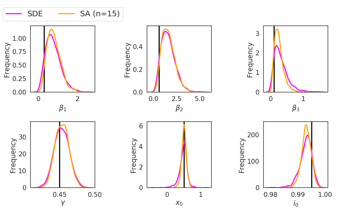
Figure 7: Simulated dataset 1: Posterior marginal densities of the parameters obtained using the SDE and the SA (with $n=15$ basis function). These densities are summarised using a kernel density estimate. The black line in each of the plots demarcate the generative parameter value.

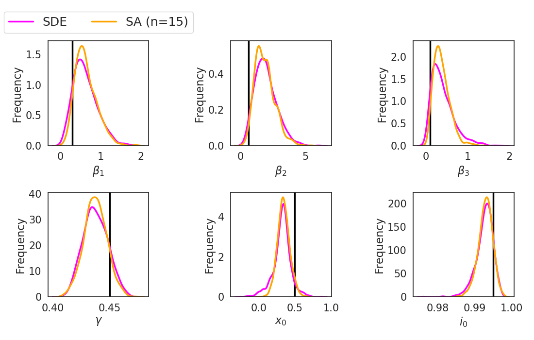
Figure 8: Simulated dataset 2: Posterior marginal densities.

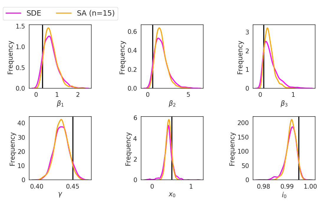
Figure 9: Simulated dataset 3: Posterior marginal densities.

In Figure 7–9 we compare the marginal densities of the parameters obtained using the SDE and SA counterparts, for each of the simulated datasets. Clearly the estimates match well and generative parameter values are recovered.

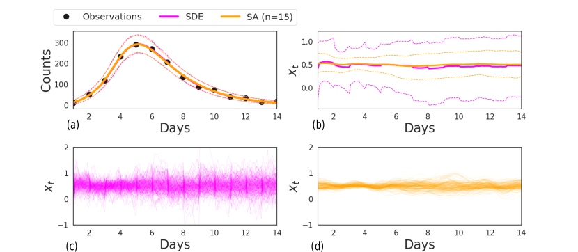
Figure 10: Simulated dataset 1: Goodness-of-fit (a); posterior distribution of the latent diffusion paths corresponding to the SDE and SA counterparts (b), with densities summarised by the mean (solid lines) and $95\%$ credible intervals (broken lines); and samples from the posterior distribution of the latent diffusion paths, SDE (c) and SA (d)

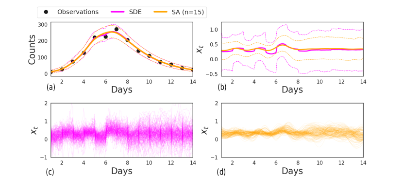
Figure 11: Simulated dataset 2: Comparison of the goodness-of-fit

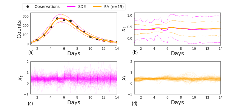
Figure 12: Simulated dataset 3: Comparison of the goodness-of-fit

Furthermore, in Figure 10–12 we compare the goodness-of-fit. As was found for the real dataset, we observe little disagreement between the epidemic curves obtained using the SDE and the SA, but for the posterior distribution of the latent diffusion paths we noticed, for all the datasets, that the credible intervals are narrower for the SA. For all these datasets, the posterior means, and the draws of the sample path, of the two models match well.

Appendix D: Calculating a time-varying reproduction number

The estimate of the contact-rate $\beta_{t_{k},r}$ is used to derive an estimate of a time-varying reproduction number. Firstly, using the formula of Wearing et al., (2005), the initial reproduction number $R_{0,r}$ is estimated as follows:

$$R_{0,r}=\psi_{r}d_{I}\frac{\left(\frac{\psi_{r}d_{L}}{2}+1\right)^{2}}{1-\frac{1}{\left(\frac{\psi_{r}d_{I}}{2}+1\right)^{2}}}.$$ (35)

Over time the value of the reproduction number will change as contact patterns shift and the supply of susceptible individuals deplete. The time-$t$ reproduction number is then estimated using the following formula:

$$R_{t_{k},r}=\begin{cases}R_{0,r}\frac{R^{*}_{t_{k},r}}{R^{*}_{0,r}}&\text{if $t_{k}<t_{\textrm{lock}}$}\\ \beta_{t_{k},r}R_{0,r}\frac{R^{*}_{t_{k},r}}{R^{*}_{0,r}}&\text{if $t_{k}\geq t_{\textrm{lock}}$}\end{cases}$$ (36)

where $t_{\textrm{lock}}$ indicates the time-point corresponding to the lockdown. $R^{*}_{t_{k},r}$ is the dominant eigenvalue of the time $t_{k}$ next-generation matrix, $\Lambda_{k,r}$, with elements:

$$\left(\Lambda_{k,r}\right)_{ij}=S_{r,{t_{k}},i}\boldsymbol{{C}}^{t_{k}}_{r,ij}d_{I},$$ (37)

where $\boldsymbol{{C}}^{t_{k}}_{r,ij}$ is a region-specific time-varying contact matrix, see Birrell et al., (2021) for further details on these matrices.

To get an ‘all England’ value for $R_{t_{k},E}$ a weighted average of the regional $R_{t_{k},r}$ is calculated, where the weights are given by the sum of the infections in each region:

$$R_{t_{k},E}=\frac{\sum_{r}R_{t_{k},r}\sum_{i}\Delta^{\textrm{infec}}_{r,t_{k},i}}{\sum_{r}\sum_{i}\Delta^{\textrm{infec}}_{r,t_{k},i}}.$$ (38)

Appendix E: Priors for the COVID-19 model

The priors for the global and regional parameters for the COVID-19 model are listed in Table 3. We used the same priors as was used in Birrell et al., (2021). Note that we also used the same prior for the volatility of both the piecewise constant random-walk and the Brownian motion model of the transmission-potential.

Table 3: Model parameters with assumed prior distributions or fixed values, as was used in Birrell et al., (2021).

Name	Prior source
Over-dispersion, $\eta$	Uninformative $\operatorname{Gamma}(1,0.2)$.
Mean infectious period, $d_{I}$	2 + $\operatorname{Gamma}(1.43,0.549)$.
Infection-fatality rate for age $<5$: $p_{1}$	$\operatorname{Beta}(1,62110.8012)$.
Infection-fatality rate for age, $5-14$: $p_{2}$	$\operatorname{Beta}(1,23363.4859)$.
Infection-fatality rate for age $15-24$: $p_{3}$	$\operatorname{Beta}(1,5290.0052)$.
Infection-fatality rate for age $25-44$: $p_{4}$	$\operatorname{Beta}(1,1107.6474)$.
Infection-fatality rate for age $45-64$: $p_{5}$	$\operatorname{Beta}(1,120.9512)$.
Infection-fatality rate for age $65-74$: $p_{6}$	$\operatorname{Beta}(1,31.1543)$.
Infection-fatality rate for age $>74$: $p_{7}$	$\operatorname{Beta}(9.5,112)$.
Serological test sensitivity, $k_{\textrm{sens}}$	$\operatorname{Beta}(71.5,29.5)$.
Serological test specificity, $k_{\textrm{spec}}$	$\operatorname{Beta}(777.5,9.5)$.
Exponential growth, $\psi_{r}$	$\operatorname{Gamma}(31.36,224)$.
Log of initial infectives, $\log{I_{0,r}}$	$\mathcal{N}(-17.5,1.25^{2})$.
Volatility of transmission-potential, $\sigma_{\beta_{w}},\sigma_{\beta_{t}}$	$\operatorname{Gamma}(1,100)$.
Mean latent period, $d_{L}$	3 days (fixed not estimated).

Appendix F: Pseudocode of the MwG algorithm

The pseudocode listed in Algorithm 1 describes the Metropolis-within-Gibbs algorithm for sampling from the posterior distribution $p(\boldsymbol{\theta}_{g},\boldsymbol{\theta}_{1},\ldots,\boldsymbol{\theta}_{n_{r}}|\boldsymbol{y^{d}},\boldsymbol{y^{s}})$ of the global $\boldsymbol{\theta}_{g}$ and regional $\boldsymbol{\theta}_{1},\ldots,\boldsymbol{\theta}_{n_{r}}$ parameters of the COVID-19 model. For each parameter group $\boldsymbol{\theta}_{g},\boldsymbol{\theta}_{1},\ldots,\boldsymbol{\theta}_{n_{r}}$ we use a proposal with a different set of parameters that are adapted through the mechanism described in (33).

Algorithm 1 A random-scan adaptive Metropolis-within-Gibbs sampler

  Input: Number of iterations $J$; data $\boldsymbol{y^{d}},\boldsymbol{y^{s}}$; optimal acceptance rate $\bar{\alpha}$.

  Initialise the regional $\boldsymbol{\theta}^{0}_{1},\ldots,\boldsymbol{\theta}^{0}_{n_{r}}$ and global parameters $\boldsymbol{\theta}^{0}_{g}$.

  Initialise the regional proposal parameters $\lambda^{0}_{1},\ldots,\lambda^{0}_{n_{r}}$, $\boldsymbol{\mu}^{0}_{1},\ldots,\boldsymbol{\mu}^{0}_{n_{r}}$ and $\boldsymbol{\Sigma}^{0}_{1},\ldots,\boldsymbol{\Sigma}^{0}_{n_{r}}$.

  Initialise the global proposal’s parameters $\lambda^{0}_{g}$, $\boldsymbol{\mu}^{0}_{g}$ and $\boldsymbol{\Sigma}^{0}_{g}$.

  for $j=0$ to $J-1$ do

     Global move:

1. Draw $\boldsymbol{\theta}^{*}_{g}\sim\mathcal{N}(\boldsymbol{\theta}^{j}_{g},\lambda^{j}_{g}\boldsymbol{\Sigma}^{j}_{g})$ and set $\boldsymbol{\theta}^{j+1}_{g}=\boldsymbol{\theta}^{*}_{g}$ with probability $\alpha^{j}_{g}=\operatorname{min}\Big{\{}1,\frac{p(\boldsymbol{\theta}^{*}_{g}|\boldsymbol{y^{d}},\boldsymbol{y^{s}})}{p(\boldsymbol{\theta}_{g}|\boldsymbol{y^{d}},\boldsymbol{y^{s}})}\Big{\}}$, otherwise $\boldsymbol{\theta}^{j+1}_{g}=\boldsymbol{\theta}^{j}_{g}$.

     Regional move:

1. Draw $r^{*}\sim\operatorname{Uniform}(1,n_{r})$.

2. Draw $\boldsymbol{\theta}^{*}_{r^{*}}\sim\mathcal{N}(\boldsymbol{\theta}^{j}_{r^{*}},\lambda^{j}_{r^{*}}\boldsymbol{\Sigma}^{j}_{r^{*}})$ and set $\boldsymbol{\theta}^{j+1}_{r^{*}}=\boldsymbol{\theta}^{*}_{r^{*}}$ with probability $\alpha^{j}_{r^{*}}=\operatorname{min}\Big{\{}1,\frac{p(\boldsymbol{\theta}^{*}_{r^{*}}|\boldsymbol{y^{d}},\boldsymbol{y^{s}})}{p(\boldsymbol{\theta}^{j}_{r^{*}}|\boldsymbol{y^{d}},\boldsymbol{y^{s}})}\Big{\}}$, otherwise $\boldsymbol{\theta}^{j+1}_{r^{*}}=\boldsymbol{\theta}^{j}_{r^{*}}$.

3. Set $\boldsymbol{\theta}^{j+1}_{{n_{r}}\setminus{r^{*}}}=\boldsymbol{\theta}^{j}_{{n_{r}}\setminus{r^{*}}}$, where the symbol $A\setminus a$ denotes all elements of the set $A$ except $a$.

     Adaptation:

1. Adapt global proposal’s parameters:

   $$\log(\lambda^{j+1}_{g}) =\log(\lambda^{j}_{g})+\delta^{j}(\alpha^{j}_{g}-\bar{\alpha})$$ (39)

   $$\boldsymbol{\mu}^{j+1}_{g} =\boldsymbol{\mu}^{j}_{g}+\delta^{j}(\boldsymbol{\theta}^{j+1}_{g}-\boldsymbol{\mu}^{j}_{g})$$

   $$\boldsymbol{\Sigma}^{j+1}_{g} =\boldsymbol{\Sigma}^{j}_{g}+\delta^{j}(\boldsymbol{\theta}^{j+1}_{g}\boldsymbol{\theta}^{{j+1}^{{}^{\prime}}}_{g}-\boldsymbol{\Sigma}^{j}_{g}).$$

2. Adapt proposal’s parameters for region ${r^{*}}$:

   $$\log(\lambda^{j+1}_{r^{*}}) =\log(\lambda^{j}_{r^{*}})+\delta^{j}(\alpha^{j}_{r^{*}}-\bar{\alpha})$$ (40)

   $$\boldsymbol{\mu}^{j+1}_{r^{*}} =\boldsymbol{\mu}^{j}_{r^{*}}+\delta^{j}(\boldsymbol{\theta}^{j+1}_{r^{*}}-\boldsymbol{\mu}^{j}_{r^{*}})$$

   $$\boldsymbol{\Sigma}^{j+1}_{r^{*}} =\boldsymbol{\Sigma}^{j}_{r^{*}}+\delta^{j}(\boldsymbol{\theta}^{j+1}_{r^{*}}\boldsymbol{\theta}^{{j+1}^{{}^{\prime}}}_{r^{*}}-\boldsymbol{\Sigma}^{j}_{r^{*}}).$$

3. Set $\lambda^{j+1}_{{n_{r}}\setminus{r^{*}}}=\lambda^{j}_{{n_{r}}\setminus{r^{*}}}$, $\boldsymbol{\mu}^{j+1}_{{n_{r}}\setminus{r^{*}}}=\boldsymbol{\mu}^{j}_{{n_{r}}\setminus{r^{*}}}$ and $\boldsymbol{\Sigma}^{j+1}_{{n_{r}}\setminus{r^{*}}}=\boldsymbol{\Sigma}^{j}_{{n_{r}}\setminus{r^{*}}}$.

  end for

  Output: $\{\boldsymbol{\theta}^{j}_{g},\boldsymbol{\theta}^{j}_{1},\ldots,\boldsymbol{\theta}^{j}_{n_{r}}\}_{j=0}^{J-1}$.

Appendix G: Goodness-of-fit as per regions of England

In Figure 13 – 19 we show the posterior predictive distributions of the number of deaths and the posterior distribution of the latent infection for each region respectively. We have aggregated the results across ages.

Appendix H: Maximum mean discrepancy

For any given probability distribution $\mathbb{P}$ on a domain $\mathcal{X}$ its kernel embedding is defined as $\mu_{\mathbb{P}}=\mathbb{E}_{X\sim\mathbb{P}}k(\cdot,\boldsymbol{\theta})$ (Muandet et al.,, 2017), an element of reproducing kernel Hilbert space $\mathcal{H}$ associated with a positive definite kernel function $k:\mathcal{X}\times\mathcal{X}\rightarrow\mathbb{R}$. Such an embedding exists for any $\mathbb{P}$ whenever $k$ is bounded. Given two probability distributions $\mathbb{P}$ and $\mathbb{Q}$ the maximum mean discrepancy (MMD) is the Hilbert space distance between their kernel embedding $\mu_{\mathbb{P}}$ and $\mu_{\mathbb{Q}}$. Considering that we have two set of samples $\{X_{i}\}_{i=1}^{n}$ and $\{Y_{i}\}_{i=1}^{m}$ from corresponding distributions $\mathbb{P}$ and $\mathbb{Q}$ respectively, then the MMD between $\mathbb{P}$ and $\mathbb{Q}$ is given by (Gretton et al.,, 2012)

$$MMD^{2}(\mathbb{P},\mathbb{Q}) =||\mu_{\mathbb{P}}-\mu_{\mathbb{Q}}||_{\mathcal{H}}$$ (41)

$$=\frac{1}{n(n-1)}\sum_{i=1}^{n}\sum_{j\neq i}^{m}k(X_{i},X_{j})+\frac{1}{m(m-1)}\sum_{i=1}^{n}\sum_{j\neq i}^{m}k(Y_{i},Y_{j})-\frac{2}{nm}\sum_{i=1}^{n}\sum_{j=1}^{m}k(X_{i},Y_{j}).$$

The $MMD^{2}(\mathbb{P},\mathbb{Q})=0$ iff $\mathbb{P}=\mathbb{Q}$, following the properties of kernel embedding. The kernel embedding captures all the necessary information about a distribution (Muandet et al.,, 2017), thus the distance between two embedding would naturally highlight the discrepancy more efficiently in the tail regions of the distributions under comparison. In this paper we used an exponentiated quadratic kernel given by

$$k(X,X^{\prime})=\exp{\Big{(}\frac{||X-X^{\prime}||^{2}}{\rho^{2}}\Big{)}},$$ (42)

where $\rho$ is a hyperparameter. We set $\rho$ to the median distance among the samples.

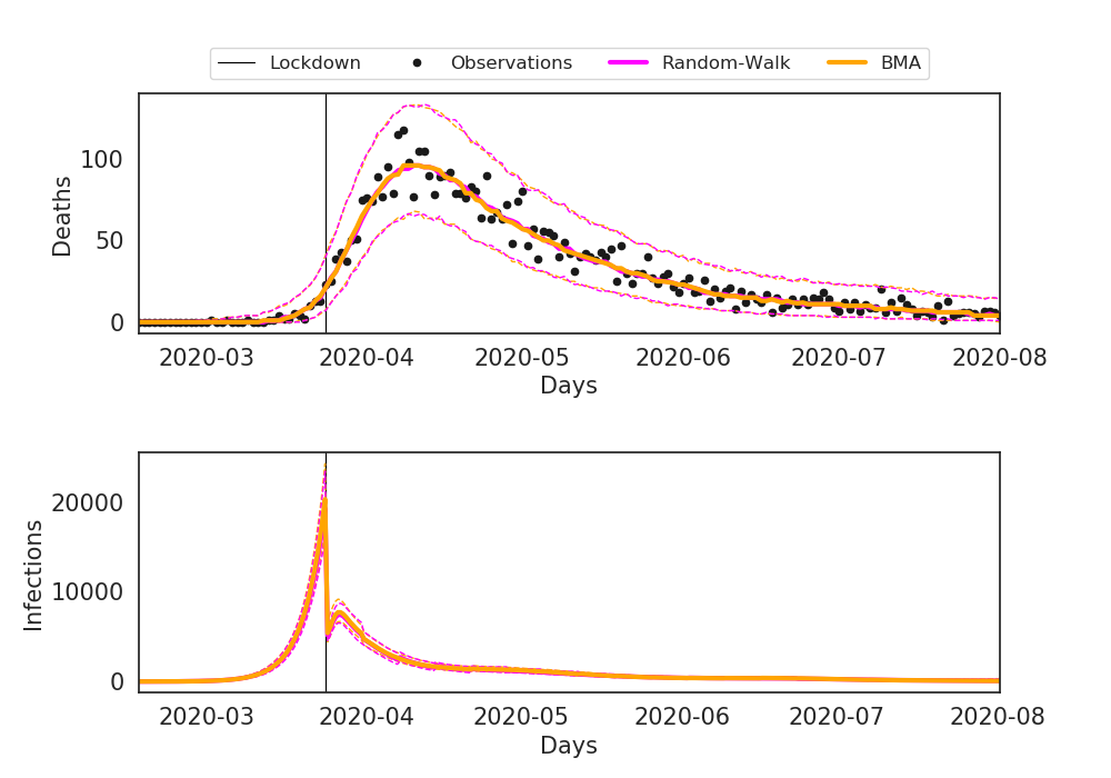
Figure 13: Goodness-of-fit of daily death data (a) and the inferred latent infections (b), produced using the random-walk (magenta lines) and BMA (orange lines) for the region East of England. These densities are summarised by the mean (solid lines) and $95\%$ credible intervals (broken lines). The black line indicates the day of lockdown in England ${23}^{\textrm{rd}}$ March, 2020.

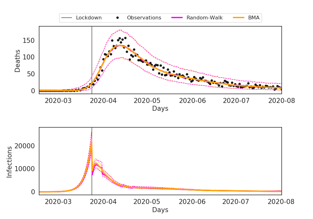
Figure 14: Goodness-of-fit of daily death data (a) and the inferred latent infections (b) for the region North West.

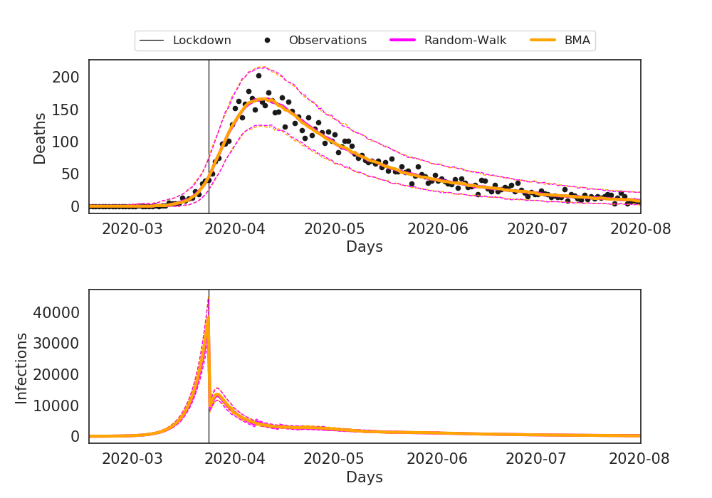
Figure 15: Goodness-of-fit of daily death data (a) and the inferred latent infections (b) for the region Midlands.

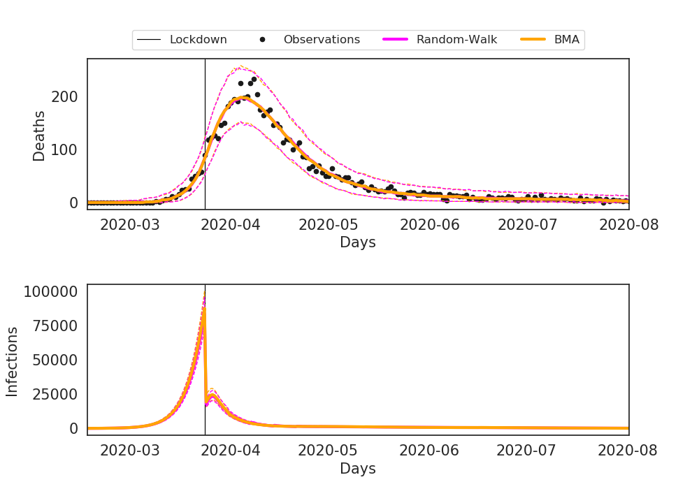
Figure 16: Goodness-of-fit of daily death data (a) and the inferred latent infections (b) for the region London.

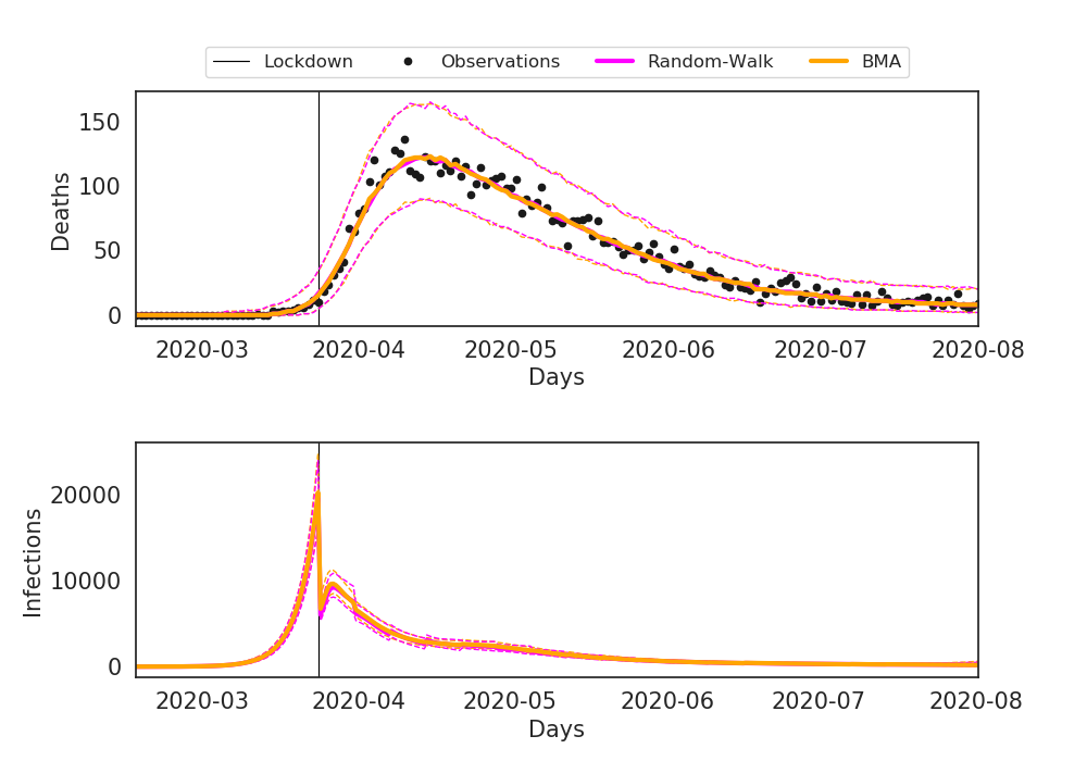
Figure 17: Goodness-of-fit of daily death data (a) and the inferred latent infections (b) for the region North East and Yorkshire.

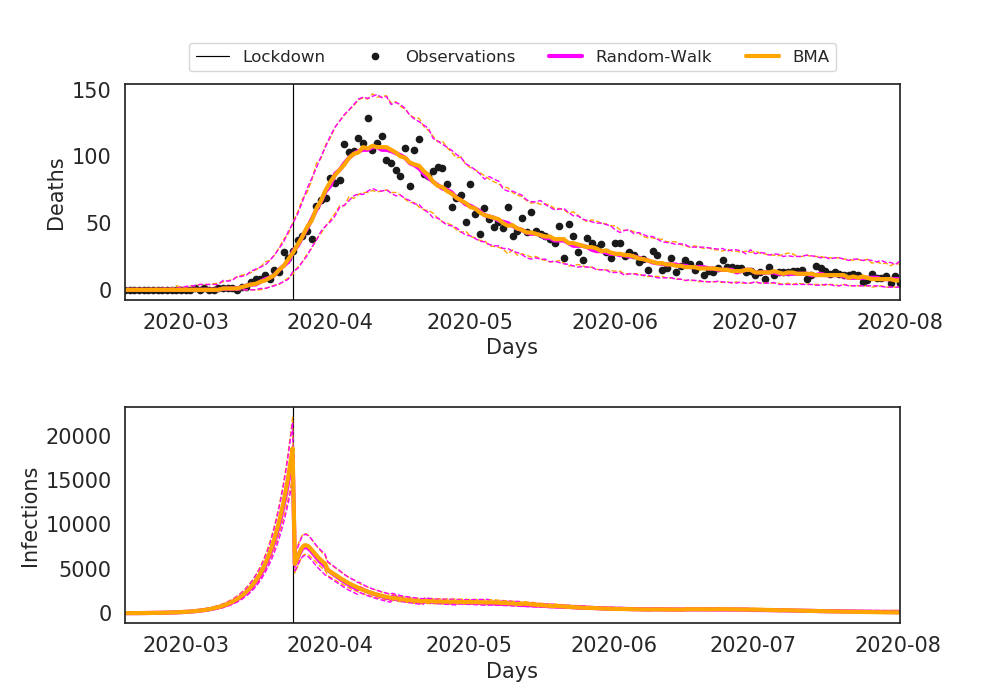
Figure 18: Goodness-of-fit of daily death data (a) and the inferred latent infections (b) for the region South East.

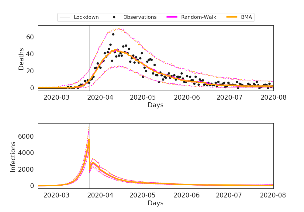
Figure 19: Goodness-of-fit of daily death data (a) and the inferred latent infections (b) for the region South West.

References

- Anderson et al., (1992) Anderson, R. M., Anderson, B., and May, R. M. (1992). Infectious diseases of humans: dynamics and control. Oxford university press.
- Andrieu and Thoms, (2008) Andrieu, C. and Thoms, J. (2008). A tutorial on adaptive mcmc. Statistics and computing, 18(4):343–373.
- Birrell et al., (2021) Birrell, P., Blake, J., Van Leeuwen, E., Gent, N., and De Angelis, D. (2021). Real-time nowcasting and forecasting of covid-19 dynamics in england: the first wave. Philosophical Transactions of the Royal Society B, 376(1829):20200279.
- Birrell et al., (2011) Birrell, P. J., Ketsetzis, G., Gay, N. J., Cooper, B. S., Presanis, A. M., Harris, R. J., Charlett, A., Zhang, X.-S., White, P. J., and Pebody, R. G. (2011). Bayesian modeling to unmask and predict influenza a/h1n1pdm dynamics in london. Proceedings of the National Academy of Sciences, 108(45):18238–18243.
- Bradbury et al., (2018) Bradbury, J., Frostig, R., Hawkins, P., Johnson, M. J., Leary, C., Maclaurin, D., Necula, G., Paszke, A., VanderPlas, J., Wanderman-Milne, S., and Zhang, Q. (2018). JAX: composable transformations of Python+NumPy programs.
- Bretó et al., (2009) Bretó, C., He, D., Ionides, E. L., and King, A. A. (2009). Time series analysis via mechanistic models. The Annals of Applied Statistics, pages 319–348.
- Brynjarsdóttir and O’Hagan, (2014) Brynjarsdóttir, J. and O’Hagan, A. (2014). Learning about physical parameters: the importance of model discrepancy. Inverse Problems, 30(11):114007.
- Cauchemez and Ferguson, (2008) Cauchemez, S. and Ferguson, N. M. (2008). Likelihood-based estimation of continuous-time epidemic models from time-series data: application to measles transmission in london. Journal of the Royal Society Interface, 5(25):885–897.
- Cauchemez et al., (2008) Cauchemez, S., Valleron, A.-J., Boelle, P.-Y., Flahault, A., and Ferguson, N. M. (2008). Estimating the impact of school closure on influenza transmission from sentinel data. Nature, 452(7188):750–754.
- Cazelles et al., (2018) Cazelles, B., Champagne, C., and Dureau, J. (2018). Accounting for non-stationarity in epidemiology by embedding time-varying parameters in stochastic models. PLoS computational biology, 14(8):e1006211.
- Cazelles and Chau, (1997) Cazelles, B. and Chau, N. (1997). Using the kalman filter and dynamic models to assess the changing hiv/aids epidemic. Mathematical biosciences, 140(2):131–154.
- Davies et al., (2020) Davies, N. G., Kucharski, A. J., Eggo, R. M., Gimma, A., Edmunds, W. J., Jombart, T., O’Reilly, K., Endo, A., Hellewell, J., and Nightingale, E. S. (2020). Effects of non-pharmaceutical interventions on covid-19 cases, deaths, and demand for hospital services in the uk: a modelling study. The Lancet Public Health, 5(7):e375–e385.
- De Angelis et al., (2015) De Angelis, D., Presanis, A. M., Birrell, P. J., Tomba, G. S., and House, T. (2015). Four key challenges in infectious disease modelling using data from multiple sources. Epidemics, 10:83–87.
- Del Moral and Murray, (2015) Del Moral, P. and Murray, L. M. (2015). Sequential monte carlo with highly informative observations. SIAM/ASA Journal on Uncertainty Quantification, 3(1):969–997.
- Dureau et al., (2013) Dureau, J., Kalogeropoulos, K., and Baguelin, M. (2013). Capturing the time-varying drivers of an epidemic using stochastic dynamical systems. Biostatistics, 14(3):541–555.
- Ellner et al., (1998) Ellner, S. P., Bailey, B., Bobashev, G. V., Gallant, A., Grenfell, B., and Nychka, D. (1998). Noise and nonlinearity in measles epidemics: combining mechanistic and statistical approaches to population modeling. The American Naturalist, 151(5):425–440.
- Fuchs, (2013) Fuchs, C. (2013). Inference for diffusion processes: with applications in life sciences. Springer Science & Business Media.
- Ghosh et al., (2022) Ghosh, S., Birrell, P. J., and De Angelis, D. (2022). Differentiable bayesian inference of sde parameters using a pathwise series expansion of brownian motion. In Proceedings of The 25th International Conference on Artificial Intelligence and Statistics, volume 151 of Proceedings of Machine Learning Research, pages 10982–10998. PMLR.
- Gordon et al., (1995) Gordon, N., Salmond, D., and Ewing, C. (1995). Bayesian state estimation for tracking and guidance using the bootstrap filter. Journal of Guidance, Control, and Dynamics, 18(6):1434–1443.
- Gretton et al., (2012) Gretton, A., Borgwardt, K. M., Rasch, M. J., Schölkopf, B., and Smola, A. (2012). A kernel two-sample test. Journal of Machine Learning Research, 13(Mar):723–773.
- Hoffman and Gelman, (2014) Hoffman, M. D. and Gelman, A. (2014). The no-u-turn sampler: adaptively setting path lengths in hamiltonian monte carlo. Journal of Machine Learning Research, 15(1):1593–1623.
- Jackson et al., (2013) Jackson, C., Vynnycky, E., Hawker, J., Olowokure, B., and Mangtani, P. (2013). School closures and influenza: systematic review of epidemiological studies. BMJ open, 3(2).
- Johnstone et al., (2016) Johnstone, R. H., Chang, E. T., Bardenet, R., De Boer, T. P., Gavaghan, D. J., Pathmanathan, P., Clayton, R. H., and Mirams, G. R. (2016). Uncertainty and variability in models of the cardiac action potential: Can we build trustworthy models? Journal of molecular and cellular cardiology, 96:49–62.
- Jombart et al., (2020) Jombart, T., Frost, S., Nouvellet, P., Campbell, F., and Sudre, B. (2020). outbreaks: A Collection of Disease Outbreak Data. R package version 1.9.0.
- Keeling et al., (2020) Keeling, M. J., Dyson, L., Guyver-Fletcher, G., Holmes, A., Semple, M. G., Tildesley, M. J., Hill, E. M., and Investigators, I. (2020). Fitting to the uk covid-19 outbreak, short-term forecasts and estimating the reproductive number. medRxiv.
- Kloeden and Eckhard, (1992) Kloeden, P. E. and Eckhard, P. (1992). Numerical Solution of Stochastic Differential Equations. springer Berlin.
- Knock et al., (2021) Knock, E. S., Whittles, L. K., Lees, J. A., Perez-Guzman, P. N., Verity, R., FitzJohn, R. G., Gaythorpe, K. A., Imai, N., Hinsley, W., and Okell, L. C. (2021). Key epidemiological drivers and impact of interventions in the 2020 sars-cov-2 epidemic in england. Science Translational Medicine.
- Luo, (2006) Luo, W. (2006). Wiener chaos expansion and numerical solutions of stochastic partial differential equations. California Institute of Technology.
- Lyons et al., (2014) Lyons, S. M., Särkkä, S., and Storkey, A. J. (2014). Series expansion approximations of brownian motion for non-linear kalman filtering of diffusion processes. IEEE Transactions on Signal Processing, 62(6):1514–1524.
- Lyons et al., (2012) Lyons, S. M. J., Storkey, A. J., and Särkkä, S. (2012). The coloured noise expansion and parameter estimation of diffusion processes. In Bartlett, P. L., Pereira, F. C. N., Burges, C. J. C., Bottou, L., and Weinberger, K. Q., editors, Advances in Neural Information Processing Systems 25: 26th Annual Conference on Neural Information Processing Systems 2012. Proceedings of a meeting held December 3-6, 2012, Lake Tahoe, Nevada, United States, pages 1961–1969.
- Martinez-Bakker et al., (2015) Martinez-Bakker, M., King, A. A., and Rohani, P. (2015). Unraveling the transmission ecology of polio. PLoS biology, 13(6):e1002172.
- Muandet et al., (2017) Muandet, K., Fukumizu, K., Sriperumbudur, B., and Schölkopf, B. (2017). Kernel mean embedding of distributions: A review and beyond. Foundations and Trends® in Machine Learning, 10(1-2):1–141.
- Oksendal, (2013) Oksendal, B. (2013). Stochastic differential equations: an introduction with applications. Springer Science & Business Media.
- Robbins and Monro, (1951) Robbins, H. and Monro, S. (1951). A stochastic approximation method. The annals of mathematical statistics, pages 400–407.
- Ryder et al., (2018) Ryder, T., Golightly, A., McGough, A. S., and Prangle, D. (2018). Black-box variational inference for stochastic differential equations. In Proceedings of the 35th International Conference on Machine Learning, pages 4423–4432.
- Sottinen and Särkkä, (2008) Sottinen, T. and Särkkä, S. (2008). Application of girsanov theorem to particle filtering of discretely observed continuous-time non-linear systems. Bayesian Analysis, 3(3):555–584.
- Wearing et al., (2005) Wearing, H. J., Rohani, P., and Keeling, M. J. (2005). Appropriate models for the management of infectious diseases. PLoS medicine, 2(7):e174.
- Wong and Zakai, (1965) Wong, E. and Zakai, M. (1965). On the Convergence of Ordinary Integrals to Stochastic Integrals. The Annals of Mathematical Statistics, 36(5):1560 – 1564.