Optimal Power Allocation for Integrated Visible Light Positioning and Communication System with a Single LED-Lamp

Abstract

In this paper, we investigate an integrated visible light positioning and communication (VLPC) system with a single LED-lamp. First, by leveraging the fact that the VLC channel model is a function of the receiver’s location, we propose a system model that estimates the channel state information (CSI) based on the positioning information without transmitting pilot sequences. Second, we derive the Cramer-Rao lower bound (CRLB) on the positioning error variance and a lower bound on the achievable rate with on-off keying modulation. Third, based on the derived performance metrics, we optimize the power allocation to minimize the CRLB, while satisfying the rate outage probability constraint. To tackle this non-convex optimization problem, we apply the worst-case distribution of the Conditional Value-at-Risk (CVaR) and the block coordinate descent (BCD) methods to obtain the feasible solutions. Finally, the effects of critical system parameters, such as outage probability, rate threshold, total power threshold, are revealed by numerical results.

I Introduction

With the explosively increasing number of Internet of Things (IoT) devices in beyond fifth generation (B5G) networks, the crisis of radio frequency (RF) spectrum shortage becomes increasingly challenging, which makes it more difficult for the RF wireless systems to meet the high speed data transmission and high accuracy positioning demands simultaneously[1]. It is worth noting that more than 50$\%$ of voice traffic and 70$\%$ of wireless data traffic occur in indoor environments [2]. Since the indoor activity requires both illumination and network access, visible light communication (VLC) [3] and visible light positioning (VLP)[4], which apply the ubiquitous light emitting diodes (LEDs) as access points (APs) and anchor nodes, are promising technologies for indoor IoT applications. Comparing with the conventional radio frequency (RF) wireless technologies, the distinct advantages of VLC and VLP are multifold [4] [5], including no electromagnetic interference, high energy efficiency, high security, and low-cost.

VLC utilizes the simple intensity modulation and direct detection (IM/DD) mechanism for information transmission, and has attracted significant research interests as a breakthrough technology for B5G networks [6]. Extensive studies have been reported to improve VLC networks performance. For example, by adopting the alternating direction method of multipliers (ADMM), a distributed coordinated interference management scheme is proposed in [7] for VLC networks. To balance energy and bandwidth efficiency, both power allocation and rate splitting are optimized in [8] for DC-biased optical orthogonal frequency division multiplexing (DCO-OFDM). In [9], in order to jointly optimize the post-equalizer, the precoder and the DC offset, a gradient projection-based procedure is presented to minimize the sum mean squared error (MSE) of the received symbols. Furthermore, VLC has been commercialized in industry. Some startup companies and existing industry giants, such as pureLiFi, Philips, and Oledcomm, are providing VLC commercial solutions in home and business buildings.

Owning to its short wavelength and low multipath interference, VLP can achieve high indoor positioning accuracy, which can facilitate various applications, such as indoor navigation, location aware services, logistic management, and assets tracking, to name few. By exploiting different visible light characteristics, existing VLP schemes can apply time of arrival (TOA) [10] [11], time difference of arrival (TDOA)[12], angle of arrival (AOA)[13] and received signal strength (RSS)[14] techniques for positioning. Among the above VLP schemes, the RSS based scheme is widely adopted due to its simplicity and ubiquity, where the distance between the lamp base station (BS) and the device is calculated based on the channel model. For example, by using the weighted k-nearest-neighbor (K-NN), a multi-LEDs positioning system is designed in [15] based on sparse fingerprints. In [16], an artificial neural network (ANN)-based position estimator is proposed for 3D RSS-based VLP systems.

Most of the existing works only focus on VLC or VLP individually. In practical indoor applications, an integrated system with both the communication and positioning functions is highly desirable. So far, only few works considered the integration of VLC and VLP. Specifically, VLC systems based on orthogonal frequency division multiplexing access (OFDMA) [17, 18] were proposed to estimate the receiver position. An integrated visible light positioning and communication (VLPC) system was designed in [19] by using filter bank multicarrier-based subcarrier multiplexing (FBMC-SCM). Such FBMC-SCM-assisted VLP with its high signal processing complexity was proposed to reduce the out-of-band interference (OOBI). Towards an OFDMA VLPC network, the authors in [20] jointly optimized the AP selection, bandwidth allocation, adaptive modulation, and power allocation to maximize the data rate while satisfying positioning accuracy constraints. In [21], a modified experience replay actor-critic (MERAC) reinforcement learning (RL) approach was presented to maximize the sum rate under the users’ minimum data rates and positioning accuracy requirements. In [22], the authors proposed a coordinated resource allocation approach to maximize the sum rate while satisfying the minimum data rates and positioning accuracy requirements of devices.

In the above considered VLPC systems, it is required that at least two lamp signals are captured at the receiver simultaneously for effective positioning. Unfortunately, such multi-lamp setup may not fit in many practical scenarios, such as in a tunnel, corridor, and staircase, where the lamps are sparsely installed. In these scenarios, the multi-lamp based method will not be as efficient as in a large and flat room. In terms of system design, most of the existing VLPC literatures [4, 23] mainly focus on optimizing the resource allocation in different frequency bands to guarantee quality of service (QoS) of communication and positioning. However, some fundamental issues have not been well investigated. Particularly, does the positioning benefit or compromise the communication? How are the two performances related? Given the limited power consumption, how to balance the two performances while taking the positioning error into account?

In this paper, we aim to address the above mentioned fundamental issues, as well as to provide a robust beamforming and power allocation scheme. The main contributions of this paper are summarized as follows:

• We establish a VLPC system model with a single LED-lamp and a mobile user with multiple photoelectric detectors (PD). By leveraging the fact that the VLC channel model is a function of the receiver’s location, the lamp estimate the channel state information (CSI) based on the positioning results, instead of transmitting pilot sequences for CSI estimation, which can significantly reduce the system overhead.

• We derive the Cramer-Rao lower bound (CRLB) on the positioning error variance, which is used as the VLP performance metric. In addition, we derive the achievable rate expression for on-off keying (OOK) modulation, and its closed-form lower bound. Furthermore, by exploiting CRLB and achievable rate expressions, we reveal the inner relationship between VLP and VLC for the first time, i.e., derive the distribution of the CSI error of VLC based on the positioning error of VLP, and obtain a rate outage probability of VLC.

• Based on the derived model and metrics, we further investigate a joint positioning and communication power allocation and beamforming problem to minimize the CRLB subject to rate outage constraints and power constraints. The outage probability constraint makes the optimization problem non-convex. Then, we apply the Conditional Value-at-Risk (CVaR) and the block coordinate descent (BCD) method techniques to convert the original problem into two convex VLP and VLC sub-problems. Finally, we develop a BCD algorithm for robust VLPC design, in which the positioning and communication power allocation are iteratively optimized until convergence.

The rest of this paper is organized as follows. We present the VLPC system model in Section II. The key performance metrics for the VLPC system are derived in Section III. In Section IV, we investigate the chance constrained robust design. Extensive simulation results are presented in Section V. Section VI concludes the paper. Moreover, Table I and II present the means of the key notations and the main acronyms of this paper, respectively.

TABLE I: Summary of Key Notations

Notation	Description
${P_{\text{p}}}$	Allocated positioning power
${P_{\text{c}}}$	Allocated communication power
${{\bf{u}}}$	Location vector of MU
${{\bf{e}}_{\rm{p}}}$	Positioning error vector
${\bf{\hat{h}}}$	Estimated CSI vector
$\Delta{\bf{h}}$	CSI estimation error vector
${\bf{I}}$	Identity matrix
${{\bf{J}}_{\rm{p}}}$	Fisher information matrix
$R_{\rm{c}}^{\rm{L}}$	Lower bound on the the achievable rate
$\mathcal{P}$	The set of distributions for ${\Delta{\bf{h}}}$
$\bar{r}$	Minimum rate requirement
${P_{{\rm{out}}}}$	Maximum tolerable outage probability

TABLE II: Summary of Main Acronyms

Notation	Description
VLP	Visible light positioning
VLC	Visible light communication
VLPC	Visible light positioning and communication
MU	Mobile user
CRLB	Cramer-Rao lower bound
CSI	Channel state information
BCD	Block coordinate descent
CVaR	Conditional Value-at-Risk

Notations: Boldfaced lowercase and uppercase letters represent vectors and matrices, respectively. $\mathcal{M}\triangleq\{1,...,M\}$. The transpose and trace of a matrix are denoted as ${\left(\cdot\right)^{\text{T}}}$ and ${\text{Tr}}\left(\cdot\right)$, respectively. ${\left\|\cdot\right\|_{2}}$ denotes 2-norm. $\mathcal{N}$ denotes the Gaussian distribution. $\bf{0}$ denotes a column vector where all elements are $0$. $\mathbb{R}^{n}$ represents the space of $n$-dimensional real matrices. $\mathbb{S}^{n}$ represents the space of $n$-dimensional real symmetric matrices.

II System Model

Figure 1: System model illustration.

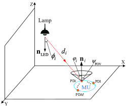
Considering a VLPC system, as shown in Fig. 1, where the lamp is equipped with a single LED that points straight downward, and a mobile user (MU) has a receiver with $M$ PDs ($M\geq 3$). Let ${\bf{l}}={\left[{{{x_{l}}},{y_{l}},{z_{l}}}\right]^{\text{T}}}$, ${{\bf{u}}}={\left[{{x_{u}},{y_{u}},{z_{u}}}\right]^{\text{T}}}$ and ${{\bf{u}}_{i}}={\left[{{x_{i}},{y_{i}},{z_{i}}}\right]^{\text{T}}}$ denote the locations of the LED, the MU and the $i$th PD, respectively, where $i\in\mathcal{M}$. Moreover, let ${{\mathbf{v}}_{i}}={\left[{{v_{x,i}},{v_{y,i}},{v_{z,i}}}\right]^{\text{T}}}$ denote the offset of the $i$th PD to the MU, i.e., ${{\mathbf{u}}_{i}}={\mathbf{u}}+{{\mathbf{v}}_{i}}$.

The wireless channel of the VLPC system has two types of links, i.e. the line-of-sight (LOS) link and the non line-of-sight (NLOS) link. Generally, the influence of the LOS link is much stronger than that of the NLOS link [24]. In order to facilitate the theoretical analysis, the design of VLPC system is based only on the LOS link, but both the LOS link and NLOS link are considered in simulation verification. According to the Lambert radiation model [25], the LOS path gain between the LED and the $i$th PD within field-of-view (FoV) can be expressed as

$${h_{i}}= \frac{{\left({m+1}\right){A_{{\rm{PD}}}}}}{{2\pi d_{i}^{2}}}{\cos^{m}}\left({{\phi_{i}}}\right)\cos\left({{\varphi_{i}}}\right)g{T_{f}}.$$ (1)

Here, $m$ is the order of Lambertian emission and $m=-\frac{{\ln 2}}{{\ln\left({\cos{\theta_{1/2}}}\right)}}$, where ${{\theta_{1/2}}}$ is the semi-angle at half power. Other parameters are defined as follows: ${A_{\text{PD}}}$ denotes the PD area; $d_{i}$ is the distance between the LED and the $i$th PD; ${\phi_{i}}$ and ${\varphi_{i}}$ are the radiance and incidence angles, respectively; $g$ denotes the gain of the optical concentrator, and is given by $g=\frac{{n_{r}^{2}}}{{{{\sin}^{2}}\left({{\psi_{\text{FoV}}}}\right)}}$, where $n_{r}$ denotes the refractive index, and ${\psi_{\text{FoV}}}$ represents the FoV of receiver; and ${T_{f}}$ denotes the gain of the optical filter.

Without loss of generality, assume that the PDs are pointing straight upward [26]. Based on the geometric relationship, the LOS path gain (1) parameters can be specified as

$${d_{i}}={\left\|{{\bf{l}}-{{\bf{u}}_{i}}}\right\|_{2}},$$ (2a)

$$\cos\left({{\phi_{i}}}\right)=\frac{{{{\left({{{\bf{u}}_{i}}-{\bf{l}}}\right)}^{\text{T}}}{{\bf{n}}_{{\rm{LED}}}}}}{{{{\left\|{{\bf{l}}-{{\bf{u}}_{i}}}\right\|}_{2}}}}=\frac{{{z_{l}}-{z_{i}}}}{{{{\left\|{{\bf{l}}-{{\bf{u}}_{i}}}\right\|}_{2}}}},$$ (2b)

$$\cos\left({{\varphi_{i}}}\right)=\frac{{{{\left({{\bf{l}}-{{\bf{u}}_{i}}}\right)}^{\text{T}}}{{\bf{n}}_{i}}}}{{{{\left\|{{\bf{l}}-{{\bf{u}}_{i}}}\right\|}_{2}}}}=\frac{{{z_{l}}-{z_{i}}}}{{{{\left\|{{\bf{l}}-{{\bf{u}}_{i}}}\right\|}_{2}}}},$$ (2c)

where ${{\bf{n}}_{{\rm{LED}}}}={\left[{0,0,-1}\right]^{\rm{T}}}$ and ${{\bf{n}}_{i}}={\left[{0,0,1}\right]^{\rm{T}}}$ are unit direction vectors of the LED and the $i$th PD, respectively. After substituting the above equations into (1), the LOS path gain can be expressed as

$${h_{i}}=\frac{{\alpha{{\left({{z_{l}}-{z_{i}}}\right)}^{m+1}}}}{{\left\|{{\bf{l}}-{{\bf{u}}_{i}}}\right\|_{2}^{m{\rm{+3}}}}},$$ (3)

where $\alpha=\frac{{\left({m+1}\right){A_{{\rm{PD}}}}g{T_{f}}}}{{2\pi}}$.

Figure 2: The frame structure of the considered VLPC system.

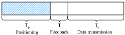
As shown in Fig. 2, the operational frame consists of three subframes: positioning subframe (downlink), feedback subframe (uplink) and data transmission subframe (downlink). The corresponding durations are ${T_{\rm{p}}}$, ${T_{\rm{u}}}$ and ${T_{\rm{c}}}$, respectively. More specific, during the positioning subframe, the LED lamp transmits the positioning symbols to the MU, which estimates the PDs’ locations based on the RSS, and the corresponding positioning information will be used for channel estimation in the next sub-frame. Then, during the feedback subframe, the MU sends feedback signals of the PDs’ locations to the lamp which estimates the CSI between the LED and the PDs. Finally, during the data transmission subframe, the lamp transmits data symbols to the MU according to the estimated CSI. This model can be extented into the multi-user system though proper multiple access methods. Due to the positioning theory, the positioning signal and subframe can be shared directly by all users without the multiple access. However, the multiple acess method, such as OFDMA, time division multiple address (TDMA), is necessary for the multi-user uplink feedback and downlink data transmission. Thus, The problem and solution also should refer to the classical theory of the multi-user networks.

II-A Positioning Signal Model and Measurements

In the following, we will specify the signal model in order to analyze the operation in each subframe. Let ${s_{{\rm{p}}}}\left(t\right)$ denote the positioning symbol generated at the lamp at time t, and $\left|{{s_{\rm{p}}}}\left(t\right)\right|\leq A$, ${\mathbb{E}}\left\{{{s_{\rm{p}}}}\left(t\right)\right\}=0$, ${\mathbb{E}}\left\{{s_{\rm{p}}^{2}}\left(t\right)\right\}=\varepsilon$, where $A>0$ is the peak amplitude.

For $t\in\left[{0,{T_{\rm{p}}}}\right]$, the transmitted positioning signal $x_{\text{p}}\left(t\right)$ of the LED is given as

$${x_{\text{p}}}\left(t\right)=\sqrt{{P_{\text{p}}}}{s_{{\rm{p}}}}\left(t\right)+{I_{{\text{DC}}}},$$ (4)

where ${P_{\text{p}}}$ indicates the allocated transmission power to the positioning symbol, and ${I_{{\text{DC}}}}>0$ denotes the direct current (DC) bias.

To guarantee that the transmitted signal is non-negative, the power $P_{\rm{p}}$ should satisfy

$$\sqrt{{P_{\rm{p}}}}A\leq{I_{{\rm{DC}}}}.$$ (5)

Given the human eye safety requirement, the LED optical power is limited, i.e.$\sqrt{{P_{\rm{p}}}}A+{I_{{\rm{DC}}}}\leq P_{\mathrm{o}}^{\max}$, where $P_{\mathrm{o}}^{\max}$ denotes the maximum optical power. Thus, the power level $P_{\rm{p}}$ should also satisfy

$$\sqrt{{P_{\rm{p}}}}\leq\frac{{P_{\mathrm{o}}^{\max}-{I_{{\rm{DC}}}}}}{A}.$$ (6)

Besides, due to practical circuit limitations, the electrical power of the transmitted signal is constrained as $\mathbb{E}\left\{{x_{\text{p}}^{2}}\left(t\right)\right\}\leq P_{\mathrm{e}}^{\max}$, i.e.,

$${P_{\rm{p}}}\varepsilon+I_{{\rm{DC}}}^{2}\leq P_{\mathrm{e}}^{\max},$$ (7)

where $P_{\mathrm{e}}^{\max}$ denotes the maximum LED electrical power.

Based on (5), (6) and (7), the constraint of the power $P_{\rm{p}}$ can be written as

$$0\leq{P_{\text{p}}}\leq\min\left\{\frac{{I_{{\rm{DC}}}^{2}}}{{{A^{2}}}},\frac{{{{\left({P_{\mathrm{o}}^{\max}-{I_{{\rm{DC}}}}}\right)}^{2}}}}{{{A^{2}}}},\frac{P_{\mathrm{e}}^{\max}-I_{{\rm{DC}}}^{2}}{\varepsilon}\right\}.$$ (8)

Then, the received positioning signal at the $i$th PD can be expressed as

$${y_{{\rm{p}},i}}\left(t\right)={h_{i}}{x_{\rm{p}}}\left(t\right)+{n_{{\rm{p}},i}}\left(t\right),$$ (9)

where $n_{{\text{p}},i}$ denotes the received additive white Gaussian noise (AWGN), which includes shot noise and thermal noise [27], and ${n_{{\rm{p}},i}}\sim{\cal N}\left({{{0}},\sigma_{\rm{p}}^{2}}\right)$.

Theoretically, the electrical power of the received positioning signal is given by

$${P_{{\rm{r}},i}}={\mathbb{E}}\left\{{y_{{\text{p}},i}^{2}}\left(t\right)\right\}=\left({{P_{\rm{p}}}\varepsilon+I_{{\rm{DC}}}^{2}}\right){h_{i}^{2}}+\sigma_{{\text{p}},i}^{2},$$ (10)

where $\sigma_{{\text{p}},i}^{2}$ denotes noise power. Combining (3) and (10), we have the following $M$ equations

$$\left\{\begin{array}[]{l}\frac{{{{\left({{z_{l}}-{z_{u}}-{v_{z,1}}}\right)}^{m+1}}}}{{\left\|{{\bf{l}}-{\bf{u}}-{{\bf{v}}_{1}}}\right\|_{2}^{m{\rm{+3}}}}}=\frac{1}{\alpha}{\left({\frac{{{P_{{\rm{r}},1}}-\sigma_{{\rm{p}},1}^{2}}}{{{P_{\rm{p}}}\varepsilon+I_{{\rm{DC}}}^{2}}}}\right)^{\frac{1}{2}}},\\ {\rm{}}\vdots\\ \frac{{{{\left({{z_{l}}-{z_{u}}-{v_{z,M}}}\right)}^{m+1}}}}{{\left\|{{\bf{l}}-{\bf{u}}-{{\bf{v}}_{M}}}\right\|_{2}^{m{\rm{+3}}}}}=\frac{1}{\alpha}{\left({\frac{{{P_{{\rm{r}},M}}-\sigma_{{\rm{p}},M}^{2}}}{{{P_{\rm{p}}}\varepsilon+I_{{\rm{DC}}}^{2}}}}\right)^{\frac{1}{2}}}.\end{array}\right.$$ (14)

To transform the Equations in (14) into a concise form, we define the auxiliary variable

$${\eta_{i}}\left({\bf{u}}\right)=\frac{{{{\left({{z_{l}}-{z_{u}}-{v_{z,i}}}\right)}^{m+1}}}}{{\left\|{{\bf{l}}-{\bf{u}}-{{\bf{v}}_{i}}}\right\|_{2}^{m{\rm{+3}}}}}-\frac{1}{\alpha}{\left({\frac{{{P_{{\rm{r}},i}}-\sigma_{{\rm{p}},i}^{2}}}{{{P_{\rm{p}}}\varepsilon+I_{{\rm{DC}}}^{2}}}}\right)^{\frac{1}{2}}}.$$ (15)

Thus, Equation (14) can be equivalently reformulated as follows

$${\eta_{i}}\left({\bf{u}}\right)=0,i\in\mathcal{M}.$$ (16)

Here Equation (16) can be solved by using off-the-shelf optimization solvers, such as FSOLVE in MATLAB[28].

In general, the positioning error is inevitable. Let ${{{\mathbf{\hat{u}}}}}$ and ${{\bf{e}}_{\rm{p}}}$ denote the estimated MU location and the corresponding positioning error, where ${{\bf{e}}_{\rm{p}}}={\left[{{e_{x}},{e_{y}},{e_{z}}}\right]^{\text{T}}}$. Their relationship can be written as

$${{\mathbf{e}}_{\text{p}}}={{\mathbf{u}}}-{{{\mathbf{\hat{u}}}}}.$$ (17)

Generally, the positioning error ${{\mathbf{e}}_{\mathrm{p}}}$ can be assumed to follow the Gaussian distribution [29, 30, 31], and then CRLB can be achieved by the maximum-likelihood (ML) estimator [32, 33]. We use $f_{\mathbf{e}_{\mathrm{p}}}\left(\mathbf{e}_{\rm{p}}\right)$ to denote the probability density distribution of ${{\bf{e}}_{\rm{p}}}$, which follows a Gaussian distribution with mean ${\bf{0}}$ and covariance matrix ${{\bf{E}}_{\rm{p}}}$, i.e., ${{\bf{e}}_{\rm{p}}}\sim{\mathcal{N}}\left({{\bf{0}},{{\bf{E}}_{\rm{p}}}}\right)$.

II-B MU Feedback and Channel Estimation

When $t\in\left[{{T_{\rm{p}}},{T_{\rm{p}}}+{T_{\rm{u}}}}\right]$, the estimated location of the MU ${{{\mathbf{\hat{u}}}}}$ will be sent to the lamp, which also serves as an anchor node. Based on ${{{\mathbf{\hat{u}}}}}$, the lamp can estimate the CSI between the LED and the PDs. Specifically, ${\bf{\hat{h}}}=\left[{{{\hat{h}}_{1}},...,{{\hat{h}}_{M}}}\right]^{\mathrm{T}}\in{\mathbb{R}^{M\times 1}}$ denotes the estimated CSI vector; $\Delta{\bf{h}}=\left[{\Delta{h_{1}},...,\Delta{h_{M}}}\right]^{\mathrm{T}}\in{\mathbb{R}^{M\times 1}}$ denotes the CSI estimation error vector.

Let ${h_{i}}$ and ${\hat{h}_{i}}$ denote the perfect and estimated CSI between the LED and the $i$th PD, and $\Delta{h_{i}}$ denote the estimated CSI error, i.e., ${h_{i}}={\hat{h}_{i}}+\Delta{h_{i}}$. According to (3), the estimated CSI ${\hat{h}_{i}}$ is a function of the estimated UE’s location ${{{\mathbf{\hat{u}}}}}$ given by

$${\hat{h}_{i}}=\frac{{\alpha{{\left({{z_{l}}-{{\hat{z}}_{u}}-{v_{z,i}}}\right)}^{m+1}}}}{{\left\|{{\bf{l}}-{\bf{\hat{u}}}-{{\bf{v}}_{i}}}\right\|_{2}^{m+3}}}.$$ (18)

Based on (3) and (18), the estimated CSI error $\Delta{h_{i}}$ is given as

$$\Delta{h_{i}}{\rm{}}=\frac{{\alpha{{\left({{z_{l}}-{{\hat{z}}_{u}}-{v_{z,i}}-{e_{z}}}\right)}^{m+1}}}}{{\left\|{{\bf{l}}-{\bf{\hat{u}}}-{{\bf{v}}_{i}}-{{\bf{e}}_{\rm{p}}}}\right\|_{2}^{m+3}}}-\frac{{\alpha{{\left({{z_{l}}-{{\hat{z}}_{u}}-{v_{z,i}}}\right)}^{m+1}}}}{{\left\|{{\bf{l}}-{\bf{\hat{u}}}-{{\bf{v}}_{i}}}\right\|_{2}^{m+3}}}.$$ (19)

II-C Data Transmission

Let ${s_{{\rm{OOK}}}}\left(t\right)$ denote the data symbol transmitted from the LED, and ${s_{{\rm{OOK}}}}\left(t\right)$ takes value $0$ or $A$ with equal probability, i.e., $\Pr\left\{{{s_{{\rm{OOK}}}}\left(t\right)=0}\right\}=\frac{1}{2}$, and ${\Pr\left\{{{s_{{\rm{OOK}}}}\left(t\right)=A}\right\}=\frac{1}{2}}$, where $A$ is the peak amplitude of the symbol. Due to $s_{\mathrm{OOK}}\geq 0$, $I_{\mathrm{DC}}$ can be $0$ in the data transmission.

For $t\in\left[{{T_{\rm{p}}}+{T_{\rm{u}}},{T_{\rm{p}}}+{T_{\rm{u}}}+{T_{\rm{c}}}}\right]$, the LED transmitted data signal $x_{\rm{c}}\left(t\right)$ can be expressed as

$${x_{\text{c}}}\left(t\right)=\sqrt{{P_{\text{c}}}}{s_{{\text{OOK}}}}\left(t\right),$$ (20)

where ${{P_{\text{c}}}}$ indicates the allocated communication power of the LED.

Similarly, the communication power ${{P_{\text{c}}}}$ should also meet the eye safety constraint, i.e. $\sqrt{{P_{\rm{c}}}}A\leq P_{\mathrm{o}}^{\max}$, where $P_{\mathrm{o}}^{\max}$ denotes the maximum optical power. Thus, the communication power $P_{\rm{c}}$ should satisfy

$$\sqrt{{P_{\rm{c}}}}\leq\frac{{P_{\mathrm{o}}^{\max}}}{A}.$$ (21)

Under practical circuit limitations, the electrical power of the transmitted signal is constrained as $\mathbb{E}\left\{{x_{\text{c}}^{2}\left(t\right)}\right\}\leq P_{\mathrm{e}}^{\max}$, i.e.,

$${P_{\rm{c}}}\mathbb{E}\left\{{s_{{\rm{OOK}}}^{2}}\left(t\right)\right\}=\frac{P_{\mathrm{c}}A^{2}}{2}\leq P_{\mathrm{e}}^{\max},$$ (22)

where $P_{\mathrm{e}}^{\max}$ denotes the maximum LED electrical power.

Based on (21) and (22), the power $P_{\rm{c}}$ should satisfy

$$0\leq{P_{\text{c}}}\leq\min\left\{{\frac{{{{\left({P_{\mathrm{o}}^{\max}}\right)}^{2}}}}{{{A^{2}}}},\frac{{2P_{\mathrm{e}}^{\max}}}{{{A^{2}}}}}\right\}.$$ (23)

At the receiver, let ${\mathbf{v}}=\left[{{v_{1}},...,{v_{M}}}\right]^{\text{T}}\in{\mathbb{R}^{M\times 1}}$ denote the receive beamforming vector of the MU, and $\left\|{\bf{v}}\right\|=1$. Therefore, the received data signal at MU can be expressed as

$${y_{\text{c}}}\left(t\right)={{\mathbf{v}}^{\text{T}}}{\left({{\bf{\hat{h}}}+\Delta{\bf{h}}}\right)}{x_{\text{c}}}\left(t\right)+z_{\text{c}},$$ (24)

where $z_{\text{c}}\buildrel\Delta\over{=}{{\mathbf{v}}^{\text{T}}}{{\mathbf{n}}_{\text{c}}}$, and ${{\mathbf{n}}_{\text{c}}}\in{\mathbb{R}^{M\times 1}}$ denotes the receiver Gaussian noise vector, i.e., ${{\bf{n}}_{\bf{c}}}\sim{\cal N}\left({{\bf{0}},\sigma_{\rm{c}}^{2}{\bf{I}}}\right)$.

III Performance Metrics

III-A Cramer-Rao Lower Bound

The CRLB represents a lower bound on the variance of the positioning estimation error. Hence, we adopt CRLB as the performance metric for the positioning accuracy in this paper. Specifically, we consider three-dimensional MU location estimation. Considering the received signal model in (9), the likelihood function of ${{y_{{\rm{p}},i}}}\left(t\right)$ can be written as

$$f\left({{y_{{\text{p}},i}}\left(t\right);{{\mathbf{u}}}}\right)=\frac{1}{{\sqrt{2\pi}{\sigma_{\rm{p}}}}}{e^{-\frac{{{{\left({{y_{{\rm{p}},i}}\left(t\right)-{h_{i}}{x_{\rm{p}}}\left(t\right)}\right)}^{2}}}}{{2\sigma_{\rm{p}}^{2}}}}}.$$ (25)

Therefore, the log-likelihood function of the received signal $\left\{{{y_{{\rm{p}},i}}}\left(t\right)\right\}_{i}^{M}$ is obtained as follows [34]

$$\Lambda\left({{{\mathbf{u}}}}\right) =\ln\left(\mathop{\prod}\limits_{i=1}^{M}f\left({{y_{{\text{p}},i}}\left(t\right);{{\mathbf{u}}}}\right)\right)$$

$$=\ln\kappa-\frac{1}{{2{\sigma_{\rm{p}}^{2}}}}\sum\limits_{i=1}^{M}{\int_{0}^{T_{\rm{p}}}{{{\left({{y_{{\text{p}},i}}\left(t\right)-{h_{i}}{x_{\text{p}}}\left(t\right)}\right)}^{2}}\,\mathrm{d}t}},$$ (26)

where $\kappa$ is a constant that does not depend on the unknown parameters. Recalling the definition given in (17), and denoting by ${{\bf{E}}_{\rm{p}}}$ the covariance matrix of the positioning error ${{{\bf{e}}_{\rm{p}}}}$. Then, according to the definition of the CRLB on the variance of any unbiased estimator [35], a lower limit on the variance of the $i$th element in an unbiased estimate vector ${\mathbf{\hat{u}}}$ is given by

$$\sum_{i}{\left[{{{\bf{E}}_{\rm{p}}}}\right]_{ii}}\geq\sum_{i}{\left[{{\bf{J}}_{\rm{p}}^{-1}}\right]_{ii}},$$ (27)

where ${\left[\cdot\right]_{ii}}$ denotes the diagonal element of a matrix, and ${\bf{J}}_{\rm{p}}$ denotes the Fisher Information matrix (FIM), which is defined as

$${\left[{{{\mathbf{J}}_{\text{p}}}}\right]_{ij}}=-{\mathbb{E}}\left\{{\frac{{{\partial^{2}}\Lambda\left({\mathbf{u}}\right)}}{{\partial{{\mathbf{u}}_{i}}\partial{{\mathbf{u}}_{j}}}}}\right\},$$ (28)

for $i\in\left\{1,2,3\right\}$, $j\in\left\{1,2,3\right\}$. Likewise, ${\left[\cdot\right]_{ij}}$ denotes the element on the $i$th row and $j$th column of a matrix. We show in Appendix A that the FIM for (III-A) is given by

$${\bf{J}}_{\rm{p}} =\frac{{{T_{\rm{p}}}{\left({P_{\rm{p}}}\varepsilon+I_{{\rm{DC}}}^{2}\right)}}}{{\sigma_{\rm{p}}^{2}}}{\bf{Q}},$$ (29)

where

$${\bf{Q}}=\left[{\begin{array}[]{*{20}{c}}{\sum\limits_{i=1}^{M}{\frac{{\partial{h_{i}}}}{{\partial{x_{u}}}}\frac{{\partial{h_{i}}}}{{\partial{x_{u}}}}}}&{\sum\limits_{i=1}^{M}{\frac{{\partial{h_{i}}}}{{\partial{x_{u}}}}\frac{{\partial{h_{i}}}}{{\partial{y_{u}}}}}}&{\sum\limits_{i=1}^{M}{\frac{{\partial{h_{i}}}}{{\partial{x_{u}}}}\frac{{\partial{h_{i}}}}{{\partial{z_{u}}}}}}\\ {\sum\limits_{i=1}^{M}{\frac{{\partial{h_{i}}}}{{\partial{x_{u}}}}\frac{{\partial{h_{i}}}}{{\partial{y_{u}}}}}}&{\sum\limits_{i=1}^{M}{\frac{{\partial{h_{i}}}}{{\partial{y_{u}}}}\frac{{\partial{h_{i}}}}{{\partial{y_{u}}}}}}&{\sum\limits_{i=1}^{M}{\frac{{\partial{h_{i}}}}{{\partial{y_{u}}}}\frac{{\partial{h_{i}}}}{{\partial{z_{u}}}}}}\\ {\sum\limits_{i=1}^{M}{\frac{{\partial{h_{i}}}}{{\partial{x_{u}}}}\frac{{\partial{h_{i}}}}{{\partial{z_{u}}}}}}&{\sum\limits_{i=1}^{M}{\frac{{\partial{h_{i}}}}{{\partial{y_{u}}}}\frac{{\partial{h_{i}}}}{{\partial{z_{u}}}}}}&{\sum\limits_{i=1}^{M}{\frac{{\partial{h_{i}}}}{{\partial{z_{u}}}}\frac{{\partial{h_{i}}}}{{\partial{z_{u}}}}}}\end{array}}\right],$$ (30d)

$$\frac{{\partial{h_{i}}}}{{\partial{x_{u}}}}=\frac{{-\alpha\left({m+3}\right){{\left({{z_{l}}-{z_{u}}-{v_{z,i}}}\right)}^{m+1}}\left({{x_{u}}+{v_{x,i}}-{x_{l}}}\right)}}{{{{\left\|{{\bf{l}}-{\bf{u}}-{{\bf{v}}_{i}}}\right\|}^{m+5}}}},$$ (30e)

$$\frac{{\partial{h_{i}}}}{{\partial{y_{u}}}}=\frac{{-\alpha\left({m+3}\right){{\left({{z_{l}}-{z_{u}}-{v_{z,i}}}\right)}^{m+1}}\left({{y_{u}}+{v_{y,i}}-{y_{l}}}\right)}}{{{{\left\|{{\bf{l}}-{\bf{u}}-{{\bf{v}}_{i}}}\right\|}^{m+5}}}},$$ (30f)

$$\frac{{\partial{h_{i}}}}{{\partial{z_{u}}}}=\frac{{-\left({m+1}\right)\alpha{{\left({{z_{l}}-{z_{u}}-{v_{z,i}}}\right)}^{m}}}}{{{{\left\|{{\bf{l}}-{\bf{u}}-{{\bf{v}}_{i}}}\right\|}^{m+3}}}}$$

$$\quad\quad\quad\quad\quad\quad+\frac{{\left({m+3}\right)\alpha{{\left({{z_{l}}-{z_{u}}-{v_{z,i}}}\right)}^{m+2}}}}{{{{\left\|{{\bf{l}}-{\bf{u}}-{{\bf{v}}_{i}}}\right\|}^{m+5}}}}.$$ (30g)

Moreover, let $B$ (Hz) denote the bandwidth of VLC link. Combine the bandwidth of VLC link, the variance of positioning error ${{\bf{e}}_{\rm{p}}}$ is lower bounded by

$${\text{Tr}}\left({{{\mathbf{E}}_{\text{p}}}}\right)\geq{\text{Tr}}\left({{\mathbf{J}}_{\text{p}}^{-1}}\right)=\frac{{B\sigma_{\text{p}}^{2}{\text{Tr}}\left({{{\mathbf{Q}}^{-1}}}\right)}}{{{T_{\text{p}}}\left({{P_{\text{p}}}\varepsilon+I_{{\text{DC}}}^{2}}\right)}}.$$ (31)

In the following, we will use (31) as the positioning performance metric which is to be minimized.

III-B Achievable Rate for OOK

When considering OOK modulation, the input signal no longer follows the Gaussian distribution, and thus the Shannon capacity formula based on the Gaussian assumption cannot be directly applied. In Appendix B, we show that the mutual information is given by

$$I\left({{x_{\text{c}}};{y_{{\text{c}}}}}\right)=-\frac{1}{2}{\mathbb{E}_{{z_{\rm{c}}}}}\left\{{{{\log}_{2}}\left({\frac{{{e^{-\frac{{z_{\rm{c}}^{2}}}{{2\sigma_{\rm{c}}^{2}}}}}+{e^{-\frac{{{{\left({{{\bf{v}}^{T}}{\bf{h}}\sqrt{{P_{\rm{c}}}}A+{z_{\rm{c}}}}\right)}^{2}}}}{{2\sigma_{\rm{c}}^{2}}}}}}}{2}}\right)}\right\}$$

$$-\frac{1}{2}{\mathbb{E}_{{z_{\rm{c}}}}}\left\{{{{\log}_{2}}\left({\frac{{{e^{-\frac{{z_{\rm{c}}^{2}}}{{2\sigma_{\rm{c}}^{2}}}}}+{e^{-\frac{{{{\left({-{{\bf{v}}^{T}}{\bf{h}}\sqrt{{P_{\rm{c}}}}A+{z_{\rm{c}}}}\right)}^{2}}}}{{2\sigma_{\rm{c}}^{2}}}}}}}{2}}\right)}\right\}-\frac{1}{{2\ln 2}}.$$ (32)

Due to the expectation operation, the expression (III-B) is not analytically tractable, and can only be calculated numerically at the expense of high computational complexity. To strike a balance between complexity and analytical tractability, we derive a closed-form lower bound on the mutual information (III-B).

Let $R_{\rm{c}}^{\rm{L}}\left({\Delta{\bf{h}}}\right)$ denote a lower bound on the achievable rate. Using Jensen’s Inequality and combining ${\bf{h}}={\bf{\hat{h}}}+\Delta{\bf{h}}$, we show in Appendix C that $R_{\rm{c}}^{\rm{L}}\left({\Delta{\bf{h}}}\right)$ with the bandwidth $B$ is given by

$$R_{\rm{c}}^{\rm{L}}\left({\Delta{\bf{h}}}\right)=3B -\frac{B}{{\ln 2}}$$

$$-2B{\log_{2}}\left({1+{e^{-\frac{{{{\left({{{\bf{v}}^{\rm{T}}}\left({{\bf{\hat{h}}}+\Delta{\bf{h}}}\right)}\right)}^{2}}{P_{\rm{c}}}{A^{2}}}}{{4B\sigma_{\rm{c}}^{2}}}}}}\right).$$ (33)

The CSI error $\Delta{\bf{h}}$ affects the achievable rate, and ${\Delta{\bf{h}}}$ is a function of the positioning error ${{{\mathbf{e}}_{\text{p}}}}$ as shown in Equation (19), which also depends on the positioning signal power ${P_{\text{p}}}$. Therefore, both the positioning signal power ${P_{\text{p}}}$ and communication signal power ${P_{\text{c}}}$ affect the achievable rate, and their allocations need to be carefully optimized.

IV Robust Power Allocation for VLPC Design

In this section, we investigate the positioning error variance minimization problem via a robust power allocation design by considering the rate outage probability constraint. Different from existing works, this paper considers the application of the VLPC system in the 3D case, and establishes the connection between the rate outage probability and the positioning error for the first time.

IV-A Problem Formulation

We derive the rate outage probability by investigating the relationship between the positioning error and CSI error. Based on (19), the CSI error ${\Delta{\bf{h}}}$ is a function of the positioning error ${{{\mathbf{e}}_{\text{p}}}}$. Thus, let $\Delta{h_{i}}\buildrel\Delta\over{=}g_{i}\left({{\bf{e}}_{\rm{p}}}\right)$ denote the CSI error function of the $i$th PD, i.e.,

$$\Delta{h_{i}}={g_{i}}\left({{{\bf{e}}_{\rm{p}}}}\right)= \frac{{\alpha{{\left({{z_{l}}-{{\hat{z}}_{u}}-{v_{z,i}}-{e_{z}}}\right)}^{m+1}}}}{{\left\|{{\bf{l}}-{\bf{\hat{u}}}-{{\bf{v}}_{i}}-{{\bf{e}}_{\rm{p}}}}\right\|_{2}^{m+3}}}$$

$$\quad\quad\quad\quad-\frac{{\alpha{{\left({{z_{l}}-{{\hat{z}}_{u}}-{v_{z,i}}}\right)}^{m+1}}}}{{\left\|{{\bf{l}}-{\bf{\hat{u}}}-{{\bf{v}}_{i}}}\right\|_{2}^{m+3}}},$$ (34)

where $i\in\mathcal{M}$.

Then, we can write ${{\bf{e}}_{\rm{p}}}=g_{i}^{-1}\left({\Delta{h_{i}}}\right)$, and the probability density function ${f_{{h_{i}}}}\left({\Delta{h_{i}}}\right)$ is given by

$${f_{{h_{i}}}}\left({\Delta{h_{i}}}\right)={f_{\bf{e}_{\mathrm{p}}}}\left({g_{i}^{-1}\left({\Delta{h_{i}}}\right)}\right)\left|{\frac{{\partial g_{i}^{-1}\left({\Delta{h_{i}}}\right)}}{{\partial\Delta{h_{i}}}}}\right|.$$ (35)

Unfortunately, an explicit expression of the function ${{\bf{e}}_{\rm{p}}}=g_{i}^{-1}\left({\Delta{h_{i}}}\right)$ is difficult to derive.

Nonetheless, we can numerically calculate both the mean and covariance matrix of the CSI error vector ${\Delta{\bf{h}}}$. Specifically, let ${\bm{\mu}}=\mathbb{E}\left\{{\Delta{\mathbf{h}}}\right\}\in{\mathbb{R}^{M\times 1}}$ denote the mean vector of the estimated CSI error ${\Delta{\bf{h}}}$, which is given as

$$\mathbb{E}\left\{{\Delta{{h_{i}}}}\right\}=\int{{g_{i}}\left({{{\bf{e}}_{\rm{p}}}}\right){{f_{{{\bf{e}_{\mathrm{p}}}}}}\left({{\bf{e}}_{\rm{p}}}\right)}\,\mathrm{d}{{\bf{e}}_{\rm{p}}}}.$$ (36)

Furthermore, let ${\bf{D}}=\mathbb{E}\left\{{\left({\Delta{\bf{h}}-{\bm{\mu}}}\right){{\left({\Delta{\bf{h}}-{\bm{\mu}}}\right)}^{T}}}\right\}\in{\mathbb{R}^{M\times M}}$ denote the covariance matrix of the estimated CSI error vector ${\Delta{\bf{h}}}$. Then, the element on the $i$th row and $j$th column of ${\bf{D}}$ is given by

$${\left[{\mathbf{D}}\right]_{ij}}=\mathbb{E}\left\{\left({\Delta{h_{i}}-\mathbb{E}\left\{{\Delta{h_{i}}}\right\}}\right)\left({\Delta{h_{j}}-\mathbb{E}\left\{{\Delta{h_{j}}}\right\}}\right)\right\},$$ (37)

where $i\in\mathcal{M}$, and $j\in\mathcal{M}$.

The exact distribution of CSI errors ${\Delta{\bf{h}}}$ is unknown except for its first and second-order moments. Then, we may define a set $\mathcal{P}$ of distributions for ${\Delta{\bf{h}}}$ as follows

$$\mathcal{P}=\left\{{\mathbb{P}:{\mathbb{E}_{\mathbb{P}}}\left\{{\Delta{\bf{h}}}\right\}={\bm{\mu}},{\rm{Var}_{\mathbb{P}}}\left\{{\Delta{\bf{h}}}\right\}={\bf{D}}}\right\},$$ (38)

where $\mathbb{P}$ denotes an arbitrary distribution with the mean ${\bm{\mu}}$ and covariance matrix ${\bf{D}}$. The set $\mathcal{P}$ in (38) determines the CSI error variation, and the rate outage probability.

Now, we can formulate the positioning error variance minimization through robust power allocation problem as follows

$$\mathop{\min}\limits_{{P_{\rm{p}}},{P_{\rm{c}}},{\bf{v}}} {\rm{Tr}}\left({{\mathbf{J}}_{\text{p}}^{-1}}\right)$$ (39a)

$${\rm{s}}.{\rm{t}}. \mathop{\sup}\limits_{\Delta{\bf{h}}\sim{\mathbb{P}},~{}\mathbb{P}\in{\cal P}}\Pr\left\{{R_{\rm{c}}^{\rm{L}}\left({\Delta{\bf{h}}}\right)\leq\bar{r}}\right\}\leq{P_{{\rm{out}}}},$$ (39b)

$${P_{\rm{p}}}+{P_{\rm{c}}}\leq{{P_{\rm{T}}}},$$ (39c)

$$0\leq{P_{\text{p}}}\leq P_{\rm{p}}^{\max},$$ (39d)

$$0\leq{P_{\text{c}}}\leq P_{\rm{c}}^{\max},$$ (39e)

$$\left\|{\bf{v}}\right\|^{2}=1,$$ (39f)

where $\bar{r}$ denotes the minimum rate requirement, ${P_{{\rm{out}}}}$ denotes the maximum tolerable outage probability, ${{P_{\rm{T}}}}$ denotes the total power, $P_{\rm{p}}^{\max}\buildrel\Delta\over{=}\min\left\{\frac{{I_{{\rm{DC}}}^{2}}}{{{A^{2}}}},\frac{{{{\left({P_{\mathrm{o}}^{\max}-{I_{{\rm{DC}}}}}\right)}^{2}}}}{{{A^{2}}}},\frac{P_{\mathrm{e}}^{\max}-I_{{\rm{DC}}}^{2}}{\varepsilon}\right\}$, and $P_{\rm{c}}^{\max}\buildrel\Delta\over{=}\min\left\{{\frac{{{{\left({P_{\mathrm{o}}^{\max}}\right)}^{2}}}}{{{A^{2}}}},\frac{{2P_{\mathrm{e}}^{\max}}}{{{A^{2}}}}}\right\}$.

IV-B Proposed Robust VLPC Method

The main challenge of problem (39) lies in the chance constraint (39b), which does not have a closed-form expression. Hence, we will reformulate constraint (39b). Combined with the lower bound on the achievable rate in (III-B), the inequality ${R_{\rm{c}}^{\rm{L}}\left({\Delta{\bf{h}}}\right)\leq\bar{r}}$ can be equivalently rewritten as

$${\left({{{\bf{v}}^{\text{T}}}\left({{\bf{\hat{h}}}+\Delta{\bf{h}}}\right)}\right)^{2}}\leq\frac{\delta}{{{P_{\rm{c}}}}},$$ (40)

where $\delta\buildrel\Delta\over{=}-\frac{{4B\sigma_{\rm{c}}^{2}}}{{{A^{2}}}}\ln\left({{2^{\frac{3}{2}-\frac{1}{{2\ln 2}}-\frac{{\bar{r}}}{{2B}}}}-1}\right)$. By using the following equivalence relationship

$${\bf{V}}={\bf{v}}{{\bf{v}}^{\text{T}}}\Leftrightarrow{\bf{V}}\succeq{\bf{0}},{\rm{rank}}\left({\bf{V}}\right)=1,$$ (41)

and neglecting the non-convex rank constraint ${\rm{rank}}\left({\bf{V}}\right)=1$, constraints (40) and (39f) can be respectively relaxed as

$$\Delta{{\bf{h}}^{\text{T}}}{\bf{V}}\Delta{\bf{h}}+2{{{\bf{\hat{h}}}}^{\text{T}}}{\bf{V}}\Delta{\bf{h}}+{{{\bf{\hat{h}}}}^{\text{T}}}{\bf{V\hat{h}}}\leq\frac{\delta}{{{P_{\rm{c}}}}},$$ (42a)

$${\rm{Tr}}\left({\bf{V}}\right)=1,~{}{\bf{V}}\succeq{\bf{0}},$$ (42b)

In words, we exploit the semidefinite relaxation (SDR) technique to relax (40) to a semidefinite program (SDP). Then, the outage constraint (39b) can be recast as

$$\Pr\left\{{\Delta{{\bf{h}}^{\text{T}}}{\bf{V}}\Delta{\bf{h}}+2{{{\bf{\hat{h}}}}^{\text{T}}}{\bf{V}}\Delta{\bf{h}}+{{{\bf{\hat{h}}}}^{\text{T}}}{\bf{V\hat{h}}}-\frac{\delta}{{{P_{\rm{c}}}}}\leq 0}\right\}\leq{P_{{\rm{out}}}}.$$ (43)

An effective approach to proceed is to transform (43) into a distributionally robust chance constraint. Then, we can find the worst-case distribution among all the possible distributions from the ambiguity set, i.e.,

$${\inf_{\mathbb{P}\in\mathcal{P}}}{\mathrm{Pr}_{\mathbb{P}}} \left\{\Delta\mathbf{h}^{\mathrm{T}}(-\mathbf{V})\Delta\mathbf{h}+2\Delta\mathbf{h}^{\mathrm{T}}(-\mathbf{V})\hat{\mathbf{h}}+\hat{\mathbf{h}}^{\mathrm{T}}(-\mathbf{V})\hat{\mathbf{h}}\right.$$

$$\quad\quad\quad\quad\quad\quad\quad\quad\left.+\frac{\delta}{P_{\mathrm{c}}}\leq 0\right\}\geq 1-{P_{{\rm{out}}}},$$ (44)

where $\mathop{\inf}\limits_{\mathbb{P}\in\mathcal{P}}{\Pr_{\mathbb{P}}}\left\{\cdot\right\}$ denotes the distribution that can achieve the minimum value of the probability.

To further deal with the intractability of (IV-B), we introduce a CVaR-based method [36], which is known as a good convex approximation of the worst-case chance constraint.

$\textbf{Lemma}\ 1$ (CVaR-Based Method): For a constraint function $L$ that is concave or quadratic in ${\bm{\xi}}$, the distributionally robust chance constraint is equivalent to the worst-case constraint, given by [37]

$$\mathop{\inf}\limits_{\mathbb{P}\in\mathcal{P}}{{\Pr}_{\mathbb{P}}}\left\{{L\left({\bm{\xi}}\right)\leq 0}\right\} \geq 1-\rho$$

$$\Leftrightarrow \mathop{\sup}\limits_{\mathbb{P}\in\mathcal{P}}\left\{\mathbb{P}-{{\text{CVaR}}_{\rho}}\left\{{L\left({\bm{\xi}}\right)}\right\}\right\}\leq 0,$$ (45)

where the expression $\mathbb{P}-{{\text{CVaR}}_{\rho}}\left\{{L\left({\bm{\xi}}\right)}\right\}$ denotes the CVaR of function $L\left({\bm{\xi}}\right)$ at threshold $\rho$ under distribution $\mathbb{P}$, which is defined as

$$\mathbb{P}-{\text{CVa}}{{\text{R}}_{\rho}}\left\{{L\left({\bm{\xi}}\right)}\right\}=\mathop{\inf}\limits_{\beta\in\mathbb{R}}\left\{{\beta+\frac{1}{\rho}{\mathbb{E}_{\mathbb{P}}}\left[{{{\left({L\left({\bm{\xi}}\right)-\beta}\right)}^{+}}}\right]}\right\}.$$ (46)

Here, $\mathbb{R}$ is the set of real numbers, ${\left(z\right)^{+}}=\max\left\{{0,z}\right\}$, and $\beta\in\mathbb{R}$ is an auxiliary variable introduced by CVaR. The worst-case CVaR on the right hand side of (IV-B) can be converted into a group of SDPs, which will be shown in the following lemma.

$\textbf{Lemma}\ 2$: Let $L\left({\bm{\xi}}\right)={{\bm{\xi}}^{\text{T}}}{\mathbf{Q}}{\bm{\xi}}+{{\mathbf{q}}^{\text{T}}}{\bm{\xi}}+{{\mathbf{q}}^{0}}$ denote a quadratic function of ${\bm{\xi}}$, $\forall{\bm{\xi}}\in{\mathbb{R}^{n}}$. The worst-case CVaR can be computed as [37]

$$\mathop{\sup}\limits_{\mathbb{P}\in\mathcal{P}} \left\{\mathbb{P}-{{\text{CVaR}}_{\rho}}\left\{{L\left({\bm{\xi}}\right)}\right\}\right\}=\mathop{\min}\limits_{\beta,{\mathbf{M}}}\left\{\beta+\frac{1}{\rho}{\text{Tr}}\left({{\mathbf{\Omega M}}}\right)\right\}$$ (47a)

$${\text{s}}.{\text{t}}. {\mathbf{M}}\succeq{\mathbf{0}},{\mathbf{M}}\in{\mathbb{S}^{n+1}},$$ (47b)

$${\mathbf{M}}-\left[{\begin{array}[]{*{20}{c}}{\mathbf{Q}}&{\frac{1}{2}{\mathbf{q}}}\\ {\frac{1}{2}{\mathbf{q}}^{\mathrm{T}}}&{{{\mathbf{q}}^{0}}-\beta}\end{array}}\right]\succeq{\mathbf{0}},$$ (47e)

where ${\mathbf{M}}$ is an auxiliary matrix variable, and ${\mathbf{\Omega}}$ is a matrix defined as

$${\mathbf{\Omega}}=\left[{\begin{array}[]{*{20}{c}}{{\mathbf{\Sigma}}+{\bm{\mu}}{{\bm{\mu}}^{\text{T}}}}&{\bm{\mu}}\\ {{{\bm{\mu}}^{\text{T}}}}&{\mathbf{1}}\end{array}}\right],$$ (50)

where ${\bm{\mu}}\in{\mathbb{R}^{n}}$ and ${\mathbf{\Sigma}}\in{\mathbb{S}^{n}}$ are the mean vector and covariance matrix of random vector ${\bm{\xi}}$, respectively.

Let define the continuous quadratic function $L\left({\Delta{\bf{h}}}\right)=\Delta\mathbf{h}^{\mathrm{T}}(-\mathbf{V})\Delta\mathbf{h}+2\Delta\mathbf{h}^{\mathrm{T}}(-\mathbf{V})\hat{\mathbf{h}}+\hat{\mathbf{h}}^{\mathrm{T}}(-\mathbf{V})\hat{\mathbf{h}}+\frac{\delta}{P_{\mathrm{c}}}$. By Lemma $2$, the worst-case chance constraint in (IV-B) can be computed by the optimization problem as similarly as the problem (47). Then, according to the Lemma $1$, the problem can be equivalent to the following CVaR constraints:

$$\beta+\frac{1}{{{P_{{\rm{out}}}}}}{\rm{Tr}}\left({{\bf{\Omega M}}}\right)\leq 0,$$ (51a)

$${\bf{M}}-\left[{\begin{array}[]{*{20}{c}}-{\bf{V}}&-{{{\bf{V}}^{\text{T}}}{\bf{\hat{h}}}}\\ -{{{{\bf{\hat{h}}}}^{\text{T}}}{\bf{V}}}&-{{{{\bf{\hat{h}}}}^{\text{T}}}{\bf{V\hat{h}}}+\frac{\delta}{{{P_{\rm{c}}}}}-\beta}\end{array}}\right]\succeq{\bf{0}},$$ (51d)

$${\bf{M}}\succeq{\bf{0}},{\bf{M}}\in{\mathbb{S}}{{}^{4}},$$ (51e)

where ${\bf{M}}$ and $\beta$ are two auxiliary variables, and

$${\bf{\Omega}}=\left[{\begin{array}[]{*{20}{c}}{{\bf{D}}+{\bm{\mu}}{{\bm{\mu}}^{\text{T}}}}&{\bm{\mu}}\\ {\bm{\mu}}^{\text{T}}&{\bf{1}}\end{array}}\right].$$

Therefore, the original distributionally chance-constrained problem (39) can be reformulated as follows

$$\mathop{\min}\limits_{{P_{\rm{p}}},{P_{\rm{c}}},{\bf{V}},{\bf{M}},\beta}\;~{} {\rm{Tr}}\left({{\bf{J}}_{\rm{p}}^{-1}}\right)$$ (52a)

$${\rm{s.t.}}~{} \eqref{robust_cons_Ptotal},\eqref{constraint_Pp},\eqref{constraint_Pc},\eqref{semidefinite V2},\eqref{CRaV_constraints1},\eqref{CRaV_constraints2},\eqref{CRaV_constraints3}.$$

Note that, problem (52) is still non-convex given that the optimization variables $P_{\rm{p}}$ and ${{\bf{V}}}$ are coupled together in constraint (51a). However, the problem (52) can be decomposed into two convex subproblems with two decoupling variables blocks: $\left\{{{P_{\rm{c}}},{\bf{V}},{\bf{M}},\beta}\right\}$ and ${P_{\rm{p}}}$, respectively. It means that when one of blocks is fixed, the problem becomes convex in the remaining block of variables, which is called the multi-convex problem[38]. To solve this kind of multi-convex problem, we propose an efficient BCD algorithm [39] for robust VLPC design with variables coupling, which can guarantee to globally converge to the stationary point [40, 41]. Then, at every iteration, the two convex subproblems, i.e., VLP subproblems and VLC subproblems, are alternatively optimized with respect to one block variable while the remaining blocks are held fixed. More specifically, for the $k$th iteration, the VLP and VLC subproblems are optimized follows.

IV-B1 VLP subproblem

For fixing variables $P_{\mathrm{c}}^{\left({k-1}\right)}$, the positioning power $P_{\rm{p}}^{\left({k}\right)}$ is updated via solving the following convex VLP subproblem

$$\mathop{\min}\limits_{{P_{\rm{p}}}} ~{}{\rm{Tr}}\left({{\bf{J}}_{\rm{p}}^{-1}}\right)$$ (53)

$${\rm{s}}.{\rm{t}}. ~{}\eqref{robust_cons_Ptotal},~{}\eqref{constraint_Pp},$$

which can be solved using the interior point methods, such as CVX [42].

IV-B2 VLC subproblem

With given positioning power $P_{\rm{p}}^{\left({k}\right)}$, the block variables $\left\{P_{\mathrm{c}}^{\left({k}\right)},{\bf{V}}^{\left({k}\right)},\mathbf{M}^{\left(k\right)},\beta^{\left(k\right)}\right\}$ are updated by solving the following convex VLC subproblem

$$\mathop{\min}\limits_{{P_{\rm{c}}},{\bf{V}},{\bf{M}},\beta} ~{}{P_{\rm{c}}}$$ (54)

$${\rm{s}}.{\rm{t}}. ~{}\eqref{constraint_Pc},~{}\eqref{semidefinite V2},~{}\eqref{CRaV_constraints1},~{}\eqref{CRaV_constraints2},~{}\eqref{CRaV_constraints3}.$$

In summary, the overall BCD algorithm for robust VLPC design is listed in Algorithm 1. The solution of the BCD Algorithm 1 is a stationary point of the joint optimization problem (39) [43, 44]. Note that, due to the SDR, the rank of ${{{\bf{V}}^{{\left(k\right)}}}}$ may not be $1$. For ${\rm{rank}}\left({{{\bf{V}}^{{\left(k\right)}}}}\right)=1$, the optimal beamformer $\bf{v}$ can be calculated by eigenvalue decomposition. When ${\rm{rank}}\left({{{\bf{V}}^{{\left(k\right)}}}}\right)>1$, we can calculate a high-quality feasible solution $\bf{v}$ of problem (54) based on the Gaussian randomization procedure [45]. Meanwhile, the two SDP problem can be efficiently solved with a worst case complexity $\mathcal{O}\left(\max\left\{m,n\right\}^{4}n^{0.5}\log\delta^{-1}\right)$, where $n$ is the problem size $n$, $m$ denotes the number of constraints $m$, and $\delta$ represents the accuracy of SDP [45]. And the proposed BCD algorithm has a sub-linear convergence rate, $\mathcal{O}\left(\frac{1}{k}\right)$, where $k$ is the index of iteration [46].

Algorithm 1 Block Coordinate Descent Algorithm for Robust VLPC Design

1:Initialize ${\bar{r}}$, ${P_{{\rm{out}}}}$, $P_{\text{p}}^{\left(0\right)}$, $k=0$ and set the tolerance of accuracy $\epsilon>0$;

2:repeat

3:     $k\leftarrow k+1$;

4:     Update $\left\{P_{c}^{\left({k}\right)},{{\bf{V}}^{\left({k}\right)}},\mathbf{M}^{\left(k\right)},\beta^{\left(k\right)}\right\}$ by solving VLC subproblem (54) with fixed $P_{\rm{p}}^{\left({k-1}\right)}$;

5:     Update $P_{\rm{p}}^{\left({k}\right)}$ by solving VLP subproblem (53) with given $\left\{P_{c}^{\left({k}\right)},{{\bf{V}}^{\left({k}\right)}},\mathbf{M}^{\left(k\right)},\beta^{\left(k\right)}\right\}$;

6:until  $\left|{{\rm{Tr}}{{\left({{\bf{J}}_{\rm{p}}^{-1}}\right)}^{\left(k\right)}}-{\rm{Tr}}{{\left({{\bf{J}}_{\rm{p}}^{-1}}\right)}^{\left({k-1}\right)}}}\right|\leq\epsilon$;

7:$P_{\rm{p}}^{\left({k}\right)}$, $P_{\rm{c}}^{\left({k}\right)}$ and ${{{\bf{V}}^{{\left(k\right)}}}}$.

V Simulation results

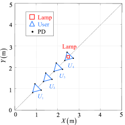
In this section, we present simulation results to evaluate the effectiveness of the proposed VLPC system design. Consider a VLPC system in a room with size $\left({5\times 5\times 3{m^{3}}}\right)$, where one corner of the room is the origin $\left({0,0,0}\right)$ of the Cartesian coordinate system $\left({X,Y,Z}\right)$. Assume that the LED location is $\left({2.5,2.5,3}\right)$ and the MU is equipped with $M=3$ PDs.

Moreover, as shown in Fig. 3, we verify the performance of the proposed optimization method for four different horizontal locations of the MU, i.e., ${U_{1}}\left({1,1,z_{u}}\right)$, ${U_{2}}\left({1.5,1.5,z_{u}}\right)$, ${U_{3}}\left({2,2,z_{u}}\right)$ and ${U_{4}}\left({2.5,2.5,z_{u}}\right)$, where the PDs are arranged according to an equilateral triangle with side length $L$. The other simulation parameters are summarized in Table III.

Figure 3: Locations of MU and LED.

TABLE III: Basic Simulation Parameters

Parameters	Value
FoV,  ${\psi_{{\rm{FoV}}}}$	${90^{\circ}}$
Detector area of PD,  $A_{\rm{PD}}$	$1{\rm{c}}{{\rm{m}}^{2}}$
Half power angle, ${\theta_{1/2}}$	${60^{\circ}}$
Gain of an optical filter, $T_{f}$	1
Gain of an optical concentrator, $g$	1
DC bias, $I_{\rm{DC}}$	2
Peak amplitude, $A$	0.007
Maximum optical power, $P_{\mathrm{o}}^{\max}$	8W
Maximum electrical power, $P_{\mathrm{e}}^{\max}$	16W
Bandwidth, $B$	$20$MHz
Noise PSD of positioning signal, $\sigma_{\rm{p}}^{2}$	${{{{10}^{-21}}{\rm{Watts}}}\mathord{\left/{\vphantom{{{{10}^{-21}}{\rm{Watts}}}{{\rm{Hz}}}}}\right.\kern-1.2pt}{{\rm{Hz}}}}$
Noise PSD of data signal, $\sigma_{\rm{c}}^{2}$	${{{{10}^{-21}}{\rm{Watts}}}\mathord{\left/{\vphantom{{{{10}^{-21}}{\rm{Watts}}}{{\rm{Hz}}}}}\right.\kern-1.2pt}{{\rm{Hz}}}}$

V-A Positioning Performance

First of all, it should be noted that the positioning error in this section is the root mean square error (RMSE), which is the error between the average estimated value obtained from multiple measurements and the true value. The positioning symbol with normalized power is considered, i.e., $\varepsilon=1$. The received SNR is defined as the received SNR at the $1$th PD, i.e, ${\rm{SNR=10lg}}\frac{{{P_{\rm{p}}}h_{1}^{2}}}{{B\sigma_{\rm{p}}^{2}}}$.

(a)

(b)

Figure 4: (a) Positioning error versus SNR when the test point is chosen at different locations, where $L=0.1m$; (b) Positioning error versus SNR when the transceiver height difference $\Delta z={z_{l}}-{z_{u}}$ is different, where $L=0.1m$.

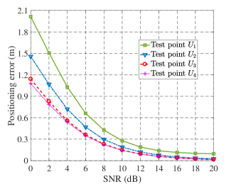
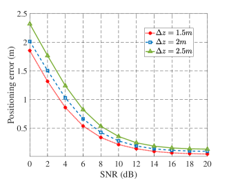
Fig. 4 (a) illustrates the positioning error at the four test points versus received SNR, where $z_{u}=1m$. We may observe that the positioning error decreases rapidly at first and then slowly, and finally converge to a constant as SNR increases. This is because as SNR increases, the influence of the noise decreases. For high SNR, the localization performance is negligibly affected by the noise, but still affected by the NLOS link. In addition, it can be seen from the Fig. 4 (a) that the positioning error at test points $U_{1}$, $U_{2}$, $U_{3}$ and $U_{4}$ gradually decreases at the same SNR. This is because $U_{4}$ is the closest to the lamp, while $U_{1}$ is the farthest. Therefore, when the total transmit power is constant, the SNR at $U_{4}$, $U_{3}$, $U_{2}$ and $U_{1}$ decreases.

In Fig. 4 (b), we plot the positioning error at test point $U_{1}$ versus SNR, for different MU heights. The shapes of the curves are similar to Fig. 4 (a), and the reasons are also similar.

Figure 5: Positioning error versus $L$(cm), where $\Delta z=2m$.

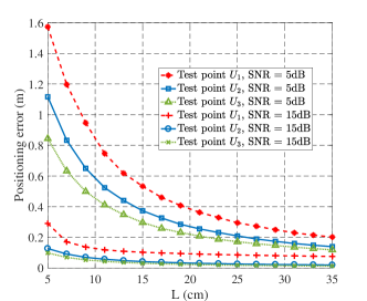
Fig. 5 shows the positioning error versus side length $L$ at high and low SNR. As we can see, with the increase of relative distance $L$, the positioning error first decreases rapidly and then slowly when the SNR=5dB, while the position error first decreases slowly and then remains unchanged when the SNR=15dB. This is because the larger the relative distance $L$ is, the greater the difference in signal intensity received by each PD will be. Thus, the solution of the nonlinear equations in (16) will be more accurate, especially at low SNR, and the impact of the signal strength difference on accuracy is more obvious. At the same time, when the relative distance $L$ reaches a certain value, additional increases will not help. In addition, when $L$ is constant, the positioning error at $U_{1}$, $U_{2}$ and $U_{3}$ still decreases sequentially, and the gap between the positioning errors at $U_{2}$ and $U_{3}$ becomes smaller with increasing $L$.

V-B Communication Performance

To evaluate the communication performance, we first introduce the non-robust VLPC design scheme, which ignores the CSI uncertainty $\Delta{\bf{h}}$, and the estimated CSI $\widehat{\bf{h}}$ is viewed as the perfect CSI ${\bf{h}}$. Moreover, in our simulations, we choose the following basic parameters: length of positioning subframe $T_{\mathrm{p}}=0.12\,\mathrm{sec}$ side length $L=0.1\,\mathrm{m}$ and the test point $U_{3}$ with $z_{u}=1.5\,\mathrm{m}$.

(a)

(b)

Figure 6: In the non-robust VLPC design, the robust VLPC design with outage probabilities ${P_{{\rm{out}}}}=1\%$ and $5\%$, and the equal power allocation design: (a)  CDF of achievable rate; (b)  CDF of CRLB.

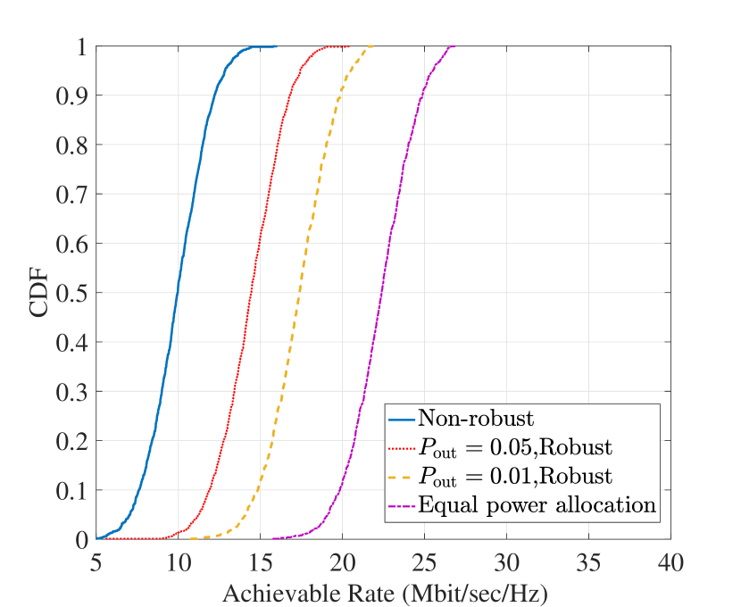
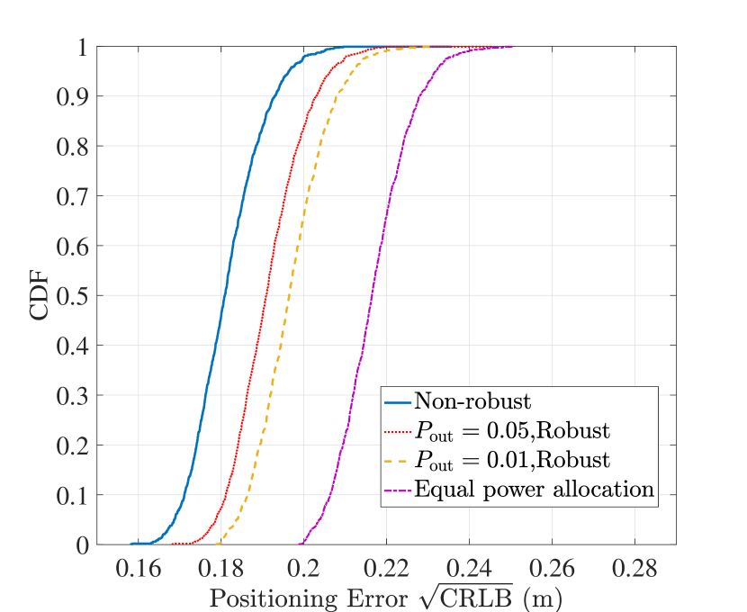
Fig. 6 (a) depicts the CDF of achievable rate of the non-robust VLPC design, the robust VLPC design with the maximum tolerated outage probabilities ${P_{{\rm{out}}}}=1\%$ and $5\%$, and the equal power allocation design (${P_{\rm{p}}}={P_{\rm{c}}}$), where the total power is ${P_{{\rm{T}}}}=10W$. It can be seen that the outage probability of the non-robust VLPC design is $50\%$, which significantly exceeds the maximum tolerated outage probability requirement. On the other hand, the outage probability of the proposed robust VLPC design is lower than $5\%$, which meets the outage probability requirement. Fig. 6 (b) depicts the CDF of CRLB with the same parameters as Fig. 6 (a). As can be seen from Fig. 6 (b), the positioning error of the robust VLPC design with ${P_{{\rm{out}}}}=1\%$ is lager than that of the design with ${P_{{\rm{out}}}}=5\%$. Combined with Fig. 6 (a), the robust VLPC design allocates more power to communication than non-robust design under the premise of minimizing positioning accuracy in order to meet the minimum rate requirements of the system. Therefore, when the total power is limited, the positioning power decreases correspondingly, resulting in the increase of positioning error. Compared with the equal power allocation scheme, the robust VLPC scheme allocates less power to communication under the condition of satisfying the rate requirement, resulting in less positioning error. Thus, Fig. 6 demonstrates the effectiveness of our proposed robust VLPC design.

Figure 7: (a)  Power allocation of robust VLPC design versus outage probability ${P_{{\rm{out}}}}$; (b)  CRLB and average communication rate ${{\tilde{R}}_{\rm{c}}}$ of robust VLPC design versus outage probability ${P_{{\rm{out}}}}$.

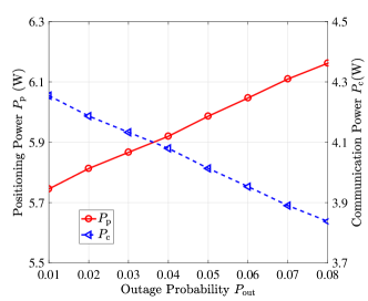
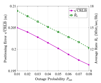
Fig. 7 (a) shows the positioning power ${P_{\rm{p}}}$ and the communication power ${P_{\rm{c}}}$ of the robust VLPC design versus the outage probability ${P_{{\rm{out}}}}$ with $\bar{r}=10{\rm{Mbit}}/\mathrm{sec}$ and ${P_{{\rm{T}}}}=10W$. From Fig. 7 (a), with increasing outage probability ${P_{{\rm{out}}}}$, the positioning power ${P_{\rm{p}}}$ increases, while the communication power ${P_{\rm{c}}}$ decreases. This is because as the outage probability ${P_{{\rm{out}}}}$ decreases, the probability that the communication rate is the threshold $\bar{r}$ decreases, and the robust design becomes more conservative. Moreover, under the same simulation conditions as Fig. 7 (a), Fig. 7 (b) depicts the CRLB and average communication rate ${{\tilde{R}}_{\rm{c}}}$ of the robust VLPC design versus the outage probability ${P_{{\rm{out}}}}$. We observe that, as the outage probability ${P_{{\rm{out}}}}$ increases, the CRLB decreases, and the average communication rate ${{\tilde{R}}_{\rm{c}}}$ also decreases. This is because for a given total power, the communication power ${P_{{\rm{c}}}}$ and the positioning power ${P_{{\rm{p}}}}$ are both related to the communication rate, and there exists a tradeoff between them.

Figure 8: (a)  Power allocation of robust VLPC design versus total power ${P_{{\rm{T}}}}$; (b)  CRLB and average rate ${{\tilde{R}}_{\rm{c}}}$ of robust VLPC design versus total power ${P_{{\rm{T}}}}$.

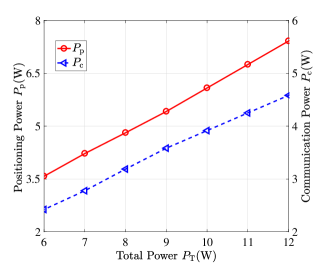
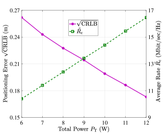
Fig. 8 show the influence of the total power ${P_{{\rm{T}}}}$ on the robust VLPC design. Fig. 8 (a) shows the optimized power allocation versus ${P_{{\rm{T}}}}$ with ${P_{{\rm{out}}}}=5\%$ and $\bar{r}=5{\rm{Mbit}}/\mathrm{sec}$. From Fig. 8 (a), we can observe that as the total power ${P_{{\rm{T}}}}$ increases, both the positioning power ${P_{\rm{p}}}$ and the communication power ${P_{\rm{c}}}$ increase because more power can be allocated for both positioning and communication power to meet the positioning performance requirements and rate constraints. In addition, Fig. 8 (b) shows the CRLB and average rate ${{\tilde{R}}_{\rm{c}}}$ versus ${P_{{\rm{T}}}}$ with the same parameters as Fig. 8 (a). From Fig. 8 (b), we can observe that as the total power ${P_{{\rm{T}}}}$ increases, the CRLB decreases and the average communication rate ${{\tilde{R}}_{\rm{c}}}$ increases. This is intuitive since higher total available power improves both the positioning and communication.

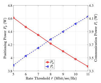
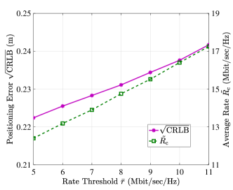
Fig. 9 show the influence of the rate thresholds $\bar{r}$ on the robust VLPC design, where ${P_{{\rm{T}}}}=8W$ and ${P_{{\rm{out}}}}=5\%$. Fig. 9 (a) shows the optimized power allocation versus different rate thresholds $\bar{r}$. We can see that the allocated positioning power ${P_{\rm{p}}}$ decreases while ${P_{\rm{c}}}$ increases as the rate threshold $\bar{r}$ increases. This is because the robust VLPC system needs more communication power to meet the rate threshold $\bar{r}$. Moreover, Fig. 9 (b) shows the CRLB and average rate ${{\tilde{R}}_{\rm{c}}}$ versus $\bar{r}$. It can be seen that as the rate threshold $\bar{r}$ increases, the CRLB increases because the positioning power ${P_{\rm{p}}}$ decreases as $\bar{r}$ increases. In addition, the average rate increases because the communication power ${P_{\rm{c}}}$ increases as $\bar{r}$ increases.

Figure 9: (a)  Power allocation of robust VLPC design versus rate threshold $\bar{r}$; (b)  CRLB and average rate ${{\tilde{R}}_{\rm{c}}}$ of robust VLPC design versus rate threshold $\bar{r}$.

VI Conclusion

In this paper, we reveal the intrinsic relationship between VLP and VLC based on the relationship between CSI and location, i.e., the positioning information can be used to estimate the CSI. Then, both the CRLB for VLP and the achievable rate of VLC are derived. Furthermore, a robust power allocation scheme is proposed under practical optical constraints, and QoS requirements. To tackle the rate outage constraints, the worst-case distribution of the CVaR is conservatively approximated to a more tractable form. Then, we propose a BCD Algorithm for robust VLPC design, in which the VLP and VLC sub-problems are iteratively optimized. Finally, our simulation results demonstrate the effectiveness of the proposed VLPC scheme for both localization and communications.

Appendix A Derivation of Equation (29)

The Fisher Information matrix (FIM) is given by

$${\mathbf{J}}_{\rm{p}}=\left[{\begin{array}[]{*{20}{c}}{-\mathbb{E}\left\{{\frac{{{\partial^{2}}\Lambda\left({\mathbf{u}}\right)}}{{\partial x_{u}^{2}}}}\right\}}&{-\mathbb{E}\left\{{\frac{{{\partial^{2}}\Lambda\left({\mathbf{u}}\right)}}{{\partial{x_{u}}\partial{y_{u}}}}}\right\}}&{-\mathbb{E}\left\{{\frac{{{\partial^{2}}\Lambda\left({\mathbf{u}}\right)}}{{\partial{x_{u}}\partial{z_{u}}}}}\right\}}\\ {-\mathbb{E}\left\{{\frac{{{\partial^{2}}\Lambda\left({\mathbf{u}}\right)}}{{\partial{y_{u}}\partial{x_{u}}}}}\right\}}&{-\mathbb{E}\left\{{\frac{{{\partial^{2}}\Lambda\left({\mathbf{u}}\right)}}{{\partial y_{u}^{2}}}}\right\}}&{-\mathbb{E}\left\{{\frac{{{\partial^{2}}\Lambda\left({\mathbf{u}}\right)}}{{\partial{y_{u}}\partial{z_{u}}}}}\right\}}\\ {-\mathbb{E}\left\{{\frac{{{\partial^{2}}\Lambda\left({\mathbf{u}}\right)}}{{\partial{z_{u}}\partial{x_{u}}}}}\right\}}&{-\mathbb{E}\left\{{\frac{{{\partial^{2}}\Lambda\left({\mathbf{u}}\right)}}{{\partial{z_{u}}\partial{y_{u}}}}}\right\}}&{-\mathbb{E}\left\{{\frac{{{\partial^{2}}\Lambda\left({\mathbf{u}}\right)}}{{\partial z_{u}^{2}}}}\right\}}\end{array}}\right].$$ (58)

Then, based on the first partial derivatives of the likelihood function in (III-A), we have

$$\frac{{\partial\Lambda\left({{{\mathbf{u}}}}\right)}}{{\partial{x_{u}}}}=-\frac{1}{{{\sigma_{\rm{p}}^{2}}}}\sum\limits_{i=1}^{M}{\int_{0}^{T_{\rm{p}}}{\left({{h_{i}}x_{\text{p}}^{2}\left(t\right)-{y_{{\text{p}},i}}\left(t\right){x_{\text{p}}}\left(t\right)}\right)\frac{{\partial{h_{i}}}}{{\partial{x_{u}}}}\,\mathrm{d}t}},$$ (59a)

$$\frac{{\partial\Lambda\left({{{\mathbf{u}}}}\right)}}{{\partial{y_{u}}}}=-\frac{1}{{{\sigma_{\rm{p}}^{2}}}}\sum\limits_{i=1}^{M}{\int_{0}^{T_{\rm{p}}}{\left({{h_{i}}x_{\text{p}}^{2}\left(t\right)-{y_{{\text{p}},i}}\left(t\right){x_{\text{p}}}\left(t\right)}\right)\frac{{\partial{h_{i}}}}{{\partial{y_{u}}}}\,\mathrm{d}t}},$$ (59b)

$$\frac{{\partial\Lambda\left({{{\mathbf{u}}}}\right)}}{{\partial{z_{u}}}}=-\frac{1}{{{\sigma^{2}}}}\sum\limits_{i=1}^{M}{\int_{0}^{T_{\rm{p}}}{\left({{h_{i}}x_{\text{p}}^{2}\left(t\right)-{y_{{\text{p}},i}}\left(t\right){x_{\text{p}}}\left(t\right)}\right)\frac{{\partial{h_{i}}}}{{\partial{z_{u}}}}\,\mathrm{d}t}}.$$ (59c)

Furthermore, according to the second partial derivatives of the likelihood function, we obtain

$$\frac{{{\partial^{2}}\Lambda\left({{{\mathbf{u}}}}\right)}}{{\partial x_{u}^{2}}} =-\frac{1}{{\sigma_{\rm{p}}^{2}}}\sum\limits_{i=1}^{M}{\int_{0}^{{T_{\rm{p}}}}{\left({\frac{{\partial{h_{i}}}}{{\partial{x_{u}}}}\frac{{\partial{h_{i}}}}{{\partial{x_{u}}}}x_{\rm{p}}^{2}\left(t\right)+{h_{i}}\frac{{{\partial^{2}}{h_{i}}}}{{\partial x_{u}^{2}}}x_{\rm{p}}^{2}\left(t\right)}\right.}}$$

$$\quad\quad\quad\quad\quad\quad\quad\left.{-{y_{{\rm{p}},i}}\left(t\right){x_{\rm{p}}}\left(t\right)\frac{{{\partial^{2}}{h_{i}}}}{{\partial x_{u}^{2}}}}\right)\,\mathrm{d}t,$$ (60a)

$$\frac{{{\partial^{2}}\Lambda\left({{{\mathbf{u}}}}\right)}}{{\partial y_{u}^{2}}} =-\frac{1}{{\sigma_{\rm{p}}^{2}}}\sum\limits_{i=1}^{M}{\int_{0}^{{T_{\rm{p}}}}{\left({\frac{{\partial{h_{i}}}}{{\partial{y_{u}}}}\frac{{\partial{h_{i}}}}{{\partial{y_{u}}}}x_{\rm{p}}^{2}\left(t\right)+{h_{i}}\frac{{{\partial^{2}}{h_{i}}}}{{\partial y_{u}^{2}}}x_{\rm{p}}^{2}\left(t\right)}\right.}}$$

$$\quad\quad\quad\quad\quad\quad\quad\left.{-{y_{{\rm{p}},i}}\left(t\right){x_{\rm{p}}}\left(t\right)\frac{{{\partial^{2}}{h_{i}}}}{{\partial y_{u}^{2}}}}\right)\,\mathrm{d}t,$$ (60b)

$$\frac{{{\partial^{2}}\Lambda\left({\bf{u}}\right)}}{{\partial z_{u}^{2}}} =-\frac{1}{{\sigma_{\rm{p}}^{2}}}\sum\limits_{i=1}^{M}{\int_{0}^{{T_{\rm{p}}}}{\left({\frac{{\partial{h_{i}}}}{{\partial{z_{u}}}}\frac{{\partial{h_{i}}}}{{\partial{z_{u}}}}x_{\rm{p}}^{2}\left(t\right)+{h_{i}}\frac{{{\partial^{2}}{h_{i}}}}{{\partial z_{u}^{2}}}x_{\rm{p}}^{2}\left(t\right)}\right.}}$$

$$\quad\quad\quad\quad\quad\quad\quad\left.{-{y_{{\rm{p}},i}}\left(t\right){x_{\rm{p}}}\left(t\right)\frac{{{\partial^{2}}{h_{i}}}}{{\partial z_{u}^{2}}}}\right)\,\mathrm{d}t,$$ (60c)

$$\frac{{{\partial^{2}}\Lambda\left({{{\mathbf{u}}}}\right)}}{{\partial{x_{u}}\partial{y_{u}}}} =\frac{{{\partial^{2}}\Lambda\left({{{\mathbf{u}}}}\right)}}{{\partial{y_{u}}\partial{x_{u}}}}=-\frac{1}{{\sigma_{\rm{p}}^{2}}}\sum\limits_{i=1}^{M}{\int_{0}^{{T_{\rm{p}}}}{\left({\frac{{\partial{h_{i}}}}{{\partial{y_{u}}}}\frac{{\partial{h_{i}}}}{{\partial{x_{u}}}}x_{\rm{p}}^{2}\left(t\right)}\right.}}$$

$$\left.{+{h_{i}}\frac{{{\partial^{2}}{h_{i}}}}{{\partial{x_{u}}\partial{y_{u}}}}x_{\rm{p}}^{2}\left(t\right)-{y_{{\rm{p}},i}}\left(t\right){x_{\rm{p}}}\left(t\right)\frac{{{\partial^{2}}{h_{i}}}}{{\partial{x_{u}}\partial{y_{u}}}}}\right)\,\mathrm{d}t,$$ (60d)

$$\frac{{{\partial^{2}}\Lambda\left({{{\mathbf{u}}}}\right)}}{{\partial{x_{u}}\partial{z_{u}}}} =\frac{{{\partial^{2}}\Lambda\left({{{\mathbf{u}}}}\right)}}{{\partial{z_{u}}\partial{x_{u}}}}=-\frac{1}{{\sigma_{\rm{p}}^{2}}}\sum\limits_{i=1}^{M}{\int_{0}^{{T_{\rm{p}}}}{\left({\frac{{\partial{h_{i}}}}{{\partial{x_{u}}}}\frac{{\partial{h_{i}}}}{{\partial{z_{u}}}}x_{\rm{p}}^{2}\left(t\right)}\right.}}$$

$$\left.{+{h_{i}}\frac{{{\partial^{2}}{h_{i}}}}{{\partial{x_{u}}\partial{z_{u}}}}x_{\rm{p}}^{2}\left(t\right)-{y_{{\rm{p}},i}}\left(t\right){x_{\rm{p}}}\left(t\right)\frac{{{\partial^{2}}{h_{i}}}}{{\partial{x_{u}}\partial{z_{u}}}}}\right)\,\mathrm{d}t,$$ (60e)

$$\frac{{{\partial^{2}}\Lambda\left({{{\mathbf{u}}}}\right)}}{{\partial{y_{u}}\partial{z_{u}}}} =\frac{{{\partial^{2}}\Lambda\left({{{\mathbf{u}}}}\right)}}{{\partial{z_{u}}\partial{y_{u}}}}=-\frac{1}{{\sigma_{\rm{p}}^{2}}}\sum\limits_{i=1}^{M}{\int_{0}^{{T_{\rm{p}}}}{\left({\frac{{\partial{h_{i}}}}{{\partial{y_{u}}}}\frac{{\partial{h_{i}}}}{{\partial{z_{u}}}}x_{\rm{p}}^{2}\left(t\right)}\right.}}$$

$$\left.{+{h_{i}}\frac{{{\partial^{2}}{h_{i}}}}{{\partial{y_{u}}\partial{z_{u}}}}x_{\rm{p}}^{2}\left(t\right)-{y_{{\rm{p}},i}}\left(t\right){x_{\rm{p}}}\left(t\right)\frac{{{\partial^{2}}{h_{i}}}}{{\partial{y_{u}}\partial{z_{u}}}}}\right)\,\mathrm{d}t.$$ (60f)

Since $\mathbb{E}\left\{{{s_{\text{p}}}}\right\}=0$, $\mathbb{E}\left\{{s_{\text{p}}^{2}}\right\}=\varepsilon$, the expectation of terms in (60) can be simplified as

$$\mathbb{E}\left\{{\frac{{{\partial^{2}}\Lambda\left({{{\mathbf{u}}}}\right)}}{{\partial x_{u}^{2}}}}\right\} =-\frac{{{T_{\rm{p}}}{\left({P_{\rm{p}}}\varepsilon+I_{{\rm{DC}}}^{2}\right)}}}{{\sigma_{\rm{p}}^{2}}}\sum\limits_{i=1}^{M}{\frac{{\partial{h_{i}}}}{{\partial{x_{u}}}}\frac{{\partial{h_{i}}}}{{\partial{x_{u}}}}},$$ (61a)

$$\mathbb{E}\left\{{\frac{{{\partial^{2}}\Lambda\left({{{\mathbf{u}}}}\right)}}{{\partial y_{u}^{2}}}}\right\} =-\frac{{{T_{\rm{p}}}{\left({P_{\rm{p}}}\varepsilon+I_{{\rm{DC}}}^{2}\right)}}}{{\sigma_{\rm{p}}^{2}}}\sum\limits_{i=1}^{M}{\frac{{\partial{h_{i}}}}{{\partial{y_{u}}}}\frac{{\partial{h_{i}}}}{{\partial{y_{u}}}}},$$ (61b)

$$\mathbb{E}\left\{{\frac{{{\partial^{2}}\Lambda\left({{{\mathbf{u}}}}\right)}}{{\partial z_{u}^{2}}}}\right\} =-\frac{{{T_{\rm{p}}}{\left({P_{\rm{p}}}\varepsilon+I_{{\rm{DC}}}^{2}\right)}}}{{\sigma_{\rm{p}}^{2}}}\sum\limits_{i=1}^{M}{\frac{{\partial{h_{i}}}}{{\partial{z_{u}}}}\frac{{\partial{h_{i}}}}{{\partial{z_{u}}}}},$$ (61c)

$$\mathbb{E}\left\{{\frac{{{\partial^{2}}\Lambda\left({{{\mathbf{u}}}}\right)}}{{\partial{x_{u}}\partial{y_{u}}}}}\right\} =\mathbb{E}\left\{{\frac{{{\partial^{2}}\Lambda\left({{{\mathbf{u}}}}\right)}}{{\partial{y_{u}}\partial{x_{u}}}}}\right\}$$

$$=-\frac{{{T_{\rm{p}}}{\left({P_{\rm{p}}}\varepsilon+I_{{\rm{DC}}}^{2}\right)}}}{{\sigma_{\rm{p}}^{2}}}\sum\limits_{i=1}^{M}{\frac{{\partial{h_{i}}}}{{\partial{x_{u}}}}\frac{{\partial{h_{i}}}}{{\partial{y_{u}}}}},$$ (61d)

$$\mathbb{E}\left\{{\frac{{{\partial^{2}}\Lambda\left({{{\mathbf{u}}}}\right)}}{{\partial{x_{u}}\partial{z_{u}}}}}\right\} =\mathbb{E}\left\{{\frac{{{\partial^{2}}\Lambda\left({{{\mathbf{u}}}}\right)}}{{\partial{z_{u}}\partial{x_{u}}}}}\right\}$$

$$=-\frac{{{T_{\rm{p}}}\left({P_{\rm{p}}}\varepsilon+I_{{\rm{DC}}}^{2}\right)}}{{\sigma_{\rm{p}}^{2}}}\sum\limits_{i=1}^{M}{\frac{{\partial{h_{i}}}}{{\partial{x_{u}}}}\frac{{\partial{h_{i}}}}{{\partial{z_{u}}}}},$$ (61e)

$$\mathbb{E}\left\{{\frac{{{\partial^{2}}\Lambda\left({{{\mathbf{u}}}}\right)}}{{\partial{y_{u}}\partial{z_{u}}}}}\right\} =\mathbb{E}\left\{{\frac{{{\partial^{2}}\Lambda\left({{{\mathbf{u}}}}\right)}}{{\partial{z_{u}}\partial{y_{u}}}}}\right\}$$

$$=-\frac{{{T_{\rm{p}}}\left({P_{\rm{p}}}\varepsilon+I_{{\rm{DC}}}^{2}\right)}}{{\sigma_{\rm{p}}^{2}}}\sum\limits_{i=1}^{M}{\frac{{\partial{h_{i}}}}{{\partial{y_{u}}}}\frac{{\partial{h_{i}}}}{{\partial{z_{u}}}}},$$ (61f)

where ${\frac{{\partial{h_{i}}}}{{\partial{x_{u}}}}}$, and ${\frac{{\partial{h_{i}}}}{{\partial{y_{u}}}}}$ and ${\frac{{\partial{h_{i}}}}{{\partial{z_{u}}}}}$ can be, respectively, expressed as

$$\frac{{\partial{h_{i}}}}{{\partial{x_{u}}}} =\frac{{-\alpha\left({m+3}\right){{\left({{z_{l}}-{z_{u}}-{v_{z,i}}}\right)}^{m+1}}\left({{x_{u}}+{v_{x,i}}-{x_{l}}}\right)}}{{{{\left\|{{\bf{l}}-{\bf{u}}-{{\bf{v}}_{i}}}\right\|}^{m+5}}}},$$ (62a)

$$\frac{{\partial{h_{i}}}}{{\partial{y_{u}}}} =\frac{{-\alpha\left({m+3}\right){{\left({{z_{l}}-{z_{u}}-{v_{z,i}}}\right)}^{m+1}}\left({{y_{u}}+{v_{y,i}}-{y_{l}}}\right)}}{{{{\left\|{{\bf{l}}-{\bf{u}}-{{\bf{v}}_{i}}}\right\|}^{m+5}}}},$$ (62b)

$$\frac{{\partial{h_{i}}}}{{\partial{z_{u}}}} =\frac{{-\left({m+1}\right)\alpha{{\left({{z_{l}}-{z_{u}}-{v_{z,i}}}\right)}^{m}}}}{{{{\left\|{{\bf{l}}-{\bf{u}}-{{\bf{v}}_{i}}}\right\|}^{m+3}}}}$$

$$\quad\quad\quad\quad\quad\quad+\frac{{\left({m+3}\right)\alpha{{\left({{z_{l}}-{z_{u}}-{v_{z,i}}}\right)}^{m+2}}}}{{{{\left\|{{\bf{l}}-{\bf{u}}-{{\bf{v}}_{i}}}\right\|}^{m+5}}}}.$$ (62c)

Appendix B Derivation of Equation (III-B)

For brevity, we drop the time index $t$ throughout this appendix. Let $s_{1}$ and $s_{2}$ denote values $A$ and $0$, respectively. According to (24), the PDF of ${{y_{{\text{c}}}}}$ can be written as

$$f\left({{y_{\rm{c}}}}\right)=\frac{1}{{2\sqrt{2\pi}{\sigma_{\rm{c}}}}}\sum\limits_{k=1}^{2}{{e^{-\frac{{{{\left({{y_{\rm{c}}}-{{\bf{v}}^{\rm{T}}}{\bf{h}}\left({\sqrt{{P_{\rm{c}}}}{s_{k}}+{I_{{\rm{DC}}}}}\right)}\right)}^{2}}}}{{2\sigma_{\rm{c}}^{2}}}}}}.$$ (63)

Then the mutual information of the receiver is derived as

$$I\left({{x_{\text{c}}};{y_{{\text{c}}}}}\right)=h\left({{y_{{\text{c}}}}}\right)-h\left({{y_{{\text{c}}}}\left|{{x_{\text{c}}}}\right.}\right)$$ (64a)

$$=-\int_{-\infty}^{\infty}{f\left({{y_{\text{c}}}}\right){{\log}_{2}}f\left({{y_{\text{c}}}}\right)\,\mathrm{d}{y_{\text{c}}}}-\frac{1}{2}{\log_{2}}2\pi e\operatorname{var}\left({z_{\text{c}}}\right)$$ (64b)

$$=-\int_{-\infty}^{\infty}{\frac{{\sum\limits_{k=1}^{2}{{e^{-\frac{{z_{\rm{c}}^{2}}}{{2\sigma_{\rm{c}}^{2}}}}}}}}{{2\sqrt{2\pi}{\sigma_{\rm{c}}}}}{{\log}_{2}}\frac{{\sum\limits_{j=1}^{2}{{e^{-\frac{{{{\left({{{\bf{v}}^{\rm{T}}}{\bf{h}}\sqrt{{P_{\rm{c}}}}\left({{s_{k}}-{s_{j}}}\right)+{z_{\rm{c}}}}\right)}^{2}}}}{{2\sigma_{\rm{c}}^{2}}}}}}}}{{2\sqrt{2\pi}{\sigma_{\rm{c}}}}}\,\mathrm{d}}{z_{\rm{c}}}$$

$$\quad\quad\quad\quad-\frac{1}{2}{\log_{2}}2\pi e\sigma_{\rm{c}}^{2}$$ (64c)

$$=-\frac{1}{2}\int_{-\infty}^{\infty}{\sum\limits_{k=1}^{2}{{f_{{z_{\rm{c}}}}}\left({{z_{\rm{c}}}}\right)}{{\log}_{2}}\frac{{\sum\limits_{j=1}^{2}{{e^{-\frac{{{{\left({{{\bf{v}}^{T}}{\bf{h}}\sqrt{{P_{\rm{c}}}}\left({{s_{k}}-{s_{j}}}\right)+{z_{\rm{c}}}}\right)}^{2}}}}{{2\sigma_{\rm{c}}^{2}}}}}}}}{{2\sqrt{2\pi}{\sigma_{\rm{c}}}}}\,\mathrm{d}{z_{\rm{c}}}}$$

$$\quad\quad\quad\quad-\frac{1}{2}{\log_{2}}2\pi e\sigma_{\rm{c}}^{2}$$ (64d)

$$=-\frac{1}{2}\sum\limits_{k=1}^{2}\mathbb{E}{{{}_{{z_{\rm{c}}}}}\left\{{{{\log}_{2}}\sum\limits_{j=1}^{2}{\frac{{{e^{-\frac{{{{\left({{{\bf{v}}^{\rm{T}}}{\bf{h}}\sqrt{{P_{\rm{c}}}}\left({{s_{k}}-{s_{j}}}\right)+{z_{\rm{c}}}}\right)}^{2}}}}{{2\sigma_{\rm{c}}^{2}}}}}}}{2}}}\right\}}$$

$$\quad\quad\quad\quad-\frac{1}{{2\ln 2}}.$$ (64e)

Appendix C Derivation of Equation (III-B)

According to Jensen’s Inequality[47], if $f\left(x\right)$ is a convex function, then we have the inequality $f\left[\mathbb{E}{\left(x\right)}\right]\geq\mathbb{E}\left[{f\left(x\right)}\right]$. Since ${\log_{2}}\left(x\right)$ is a concave function with respect to $x$, according to (64e), a lower bound on the mutual information is derived as

$$I\left({{x_{\rm{c}}};{y_{\rm{c}}}}\right)\geq-\frac{1}{2}\sum\limits_{k=1}^{2}{{{\log}_{2}}\sum\limits_{j=1}^{2}{\frac{1}{2}}\mathbb{E}{{}_{{z_{\rm{c}}}}}\left\{{{e^{-\frac{{{{\left({{{\bf{v}}^{\rm{T}}}{\bf{h}}\sqrt{{P_{\rm{c}}}}\left({{s_{k}}-{s_{j}}}\right)+{z_{\rm{c}}}}\right)}^{2}}}}{{2\sigma_{\rm{c}}^{2}}}}}}\right\}}$$

$$\quad\quad\quad\quad-\frac{1}{{2\ln 2}}$$ (65a)

$$=-\frac{1}{2}\sum\limits_{k=1}^{2}{{{\log}_{2}}\sum\limits_{j=1}^{2}{\int_{-\infty}^{\infty}{\frac{{{e^{-\frac{{{{\left({{{\bf{v}}^{\rm{T}}}{\bf{h}}\sqrt{{P_{\rm{c}}}}\left({{s_{k}}-{s_{j}}}\right)+{z_{\rm{c}}}}\right)}^{2}}+z_{\rm{c}}^{2}}}{{2\sigma_{\rm{c}}^{2}}}}}}}{2{\sqrt{2\pi}{\sigma_{\rm{c}}}}}\,\mathrm{d}{z_{\rm{c}}}}}}$$

$$\quad\quad\quad\quad-\frac{1}{{2\ln 2}}$$ (65b)

$$=-\frac{1}{2}\sum\limits_{k=1}^{2}{{{\log}_{2}}\sum\limits_{j=1}^{2}{\frac{1}{{2\sqrt{2}}}}{e^{-\frac{{{{\left({{{\bf{v}}^{\rm{T}}}{\bf{h}}\sqrt{{P_{\rm{c}}}}\left({{s_{k}}-{s_{j}}}\right)}\right)}^{2}}}}{{4\sigma_{\rm{c}}^{2}}}}}}-\frac{1}{{2\ln 2}}$$ (65c)

$$=-{\log_{2}}\left({1+{e^{-\frac{{{{\left({{{\bf{v}}^{\rm{T}}}{\bf{h}}}\right)}^{2}}{P_{\rm{c}}}{A^{2}}}}{{4\sigma_{\rm{c}}^{2}}}}}}\right)-\frac{1}{{2\ln 2}}+\frac{3}{2}.$$ (65d)

Supposed that the bandwidth of the VLC link is $B$ (Hz). Then, both the input and the output of the VLC link can be represented by samples taken $\frac{1}{{2B}}$ seconds apart. Since the power spectral density of noise is $\frac{{\sigma_{\rm{c}}^{2}}}{2}$ Watts/Hertz, the noise power is ${B\sigma_{\rm{c}}^{2}}$. For the time interval $\left[{0,T_{\rm{c}}}\right]$, there are $2BT_{\rm{c}}$ noise samples, and the variance of each sample is $\frac{{B\sigma_{\rm{p}}^{2}T_{\rm{p}}}}{{2BT_{\rm{c}}}}=\frac{{\sigma_{\rm{c}}^{2}}}{2}$. Moreover, if the power of signal is $P$, the signal energy per sample is $\frac{{PT_{\rm{c}}}}{{2BT_{\rm{c}}}}=\frac{P}{{2B}}$.

Therefore, with bandwidth $B$ and ${\bf{h}}={\bf{\hat{h}}}+\Delta{\bf{h}}$, the achievable rate is given by

$$R_{\rm{c}}^{\rm{L}}\left({\Delta{\bf{h}}}\right) =3B-\frac{B}{{\ln 2}}-2B{\log_{2}}\left({1+{e^{-\frac{{{{\left({{{\bf{v}}^{\rm{T}}}\left({{\bf{\hat{h}}}+\Delta{\bf{h}}}\right)}\right)}^{2}}{P_{\rm{c}}}{A^{2}}}}{{4B\sigma_{\rm{c}}^{2}}}}}}\right).$$ (66)

References

- [1] D. Tsonev, S. Videv, and H. Haas, “Towards a 100 Gb/s visible light wireless access network,” Opt. Express, vol. 23, no. 2, pp. 1627, 2015.
- [2] M. Weichold, M. Hamdi, M. Z. Shakir, M. Abdallah, G. K. Karagiannidis, and M. Ismail, Cognitive Radio Oriented Wireless Networks, 2015.
- [3] H. Elgala, R. Mesleh, and H. Haas, “Indoor optical wireless communication: potential and state-of-the-art,” IEEE Commun. Mag., vol. 49, no. 9, pp. 56–62, Sep. 2011.
- [4] M. F. Keskin, A. D. Sezer, and S. Gezici, “Localization via visible light systems,” Proc. IEEE, vol. 106, no. 6, pp. 1063–1088, Jun. 2018.
- [5] P. H. Pathak, X. Feng, P. Hu, and P. Mohapatra, “Visible light communication, networking, and sensing: A survey, potential and challenges,” IEEE Commun. Surv. Tutor., vol. 17, no. 4, pp. 2047–2077, 2015.
- [6] A. Jovicic, J. Li, and T. Richardson, “Visible light communication: opportunities, challenges and the path to market,” IEEE Commun. Mag., vol. 51, no. 12, pp. 26–32, Dec. 2013.
- [7] S. Ma, H. Li, Y. He, R. Yang, S. Lu, W. Cao, and S. Li, “Capacity bounds and interference management for interference channel in visible light communication networks,” IEEE Trans. Wirel. Commun., vol. 18, no. 1, pp. 182–193, Jan. 2019.
- [8] X. Deng, Mardanikorani, G. Zhou, and J. Linnartz, “DC-bias for optical OFDM in visible light communications,” IEEE Access, vol. 7, pp. 98319–98330, 2019.
- [9] Qian, Gao, Chen, Gong, Zhengyuan, and Xu, “Joint transceiver and offset design for visible light communications with input-dependent shot noise,” IEEE Trans. Wirel. Commun., vol. 16, no. 5, pp. 2736–2747, May. 2017.
- [10] C. Amini, A. Taherpour, T. Khattab, and S. Gazor, “Theoretical accuracy analysis of indoor visible light communication positioning system based on time-of-arrival,” in 2016 IEEE Canadian Conference on Electrical and Computer Engineering (CCECE), pp. 1–5, 2016.
- [11] T. Akiyama, M. Sugimoto, and H. Hashizume, “Time-of-arrival-based smartphone localization using visible light communication,” in 2017 International Conference on Indoor Positioning and Indoor Navigation(IPIN), pp. 1–7, 2017.
- [12] S. Y. Jung, S. Hann, and C. S. Park, “TDOA-based optical wireless indoor localization using LED ceiling lamps,” IEEE Trans. Consum. Electron., vol. 57, no. 4, pp. 1592–1597, Nov. 2011.
- [13] S. Yang, H. Kim, Y. Son, and S. Han, “Three-dimensional visible light indoor localization using AOA and RSS with multiple optical receivers,” J. Lightwave.Technol., vol. 32, no. 14, pp. 2480–2485, Jul. 2014.
- [14] X. Yu, J. Wang, and H. Lu, “Single LED-based indoor positioning system using multiple photodetectors,” IEEE Photon. J., vol. 10, no. 6, pp. 1–8, Dec. 2018.
- [15] A. H. A. Bakar, T. Glass, H. Y. Tee, F. Alam, and M. Legg, “Accurate visible light positioning using multiple-photodiode receiver and machine learning,” IEEE Trans. Instrum. Meas., vol. 70, pp. 1–12, 2021.
- [16] P. Du, S. Zhang, C. Chen, H. Yang, W. Zhong, R. Zhang, A. Alphones, and Y. Yang, “Experimental demonstration of 3D visible light positioning using received signal strength with low-complexity trilateration assisted by deep learning technique,” IEEE Access, vol. 7, pp. 93986–93997, 2019.
- [17] B. Lin, X. Tang, Z. Ghassemlooy, C. Lin, and Y. Li, “Experimental demonstration of an indoor VLC positioning system based on OFDMA,” IEEE Photon. J., vol. 9, no. 2, pp. 1–9, Apr. 2017.
- [18] Y. Xu, Z. Wang, P. Liu, J. Chen, S. Han, C. Yu, and J. Yu, “Accuracy analysis and improvement of visible light positioning based on VLC system using orthogonal frequency division multiple access,” Opt. Express, vol. 25, no. 26, pp. 32618–32630, Dec. 2017.
- [19] H. Yang, C. Chen, W.-D. Zhong, A. Alphones, S. Zhang, and P. Du, “Demonstration of a quasi-gapless integrated visible light communication and positioning system,” IEEE Photon. Technol. Lett., vol. 30, no. 23, pp. 2001–2004, Dec. 2018.
- [20] H. Yang, W.-D. Zhong, C. Chen, A. Alphones, and P. Du, “QoS-driven optimized design-based integrated visible light communication and positioning for indoor iot networks,” IEEE Internet Things J., vol. 7, no. 1, pp. 269–283, Jan. 2020.
- [21] H. Yang, P. Du, W.-D. Zhong, C. Chen, A. Alphones, and S. Zhang, “Reinforcement learning-based intelligent resource allocation for integrated VLCP systems,” IEEE Wireless Commun. Lett., vol. 8, no. 4, pp. 1204–1207, Aug. 2019.
- [22] H. Yang, W.-D. Zhong, C. Chen, A. Alphones, P. Du, S. Zhang, and X. Xie, “Coordinated resource allocation-based integrated visible light communication and positioning systems for indoor IoT,” IEEE Trans. Wireless Commun., vol. 19, no. 7, pp. 4671–4684, Jul. 2020.
- [23] M. F. Keskin, A. D. Sezer, and S. Gezici, “Optimal and robust power allocation for visible light positioning systems under illumination constraints,” IEEE Trans. Commun., vol. 67, no. 1, pp. 527–542, Jan. 2019.
- [24] T.Komine and M.Nakagawa, “Fundamental analysis for visible-light communication system using LED lights,” IEEE Trans. Consum.Electron., vol. 50, no. 1, pp. 100–107, Feb. 2004.
- [25] J. M. Kahn and J. R. Barry, “Wireless infrared communications,” Proc. IEEE, vol. 85, no. 2, pp. 265–298, Feb. 1997.
- [26] W. Xu, J. Wang, H. Shen, H. Zhang, and X. You, “Indoor positioning for multiphotodiode device using visible-light communications,” IEEE Photon. J., vol. 8, no. 1, pp. 1–11, Feb. 2016.
- [27] K. Sindhubala and B. Vijayalakshmi, “Simulation of vlc system under the influence of optical background noise using filtering technique,” Mater. Today: Proceedings, vol. 4, no. 2, Part B, pp. 4239–4250, 2017.
- [28] https://ww2.mathworks.cn/help/optim/ug/fsolve.html?s_tid=doc_ta.
- [29] T. Wang, G. Leus, and L. Huang, “Ranging energy optimization for robust sensor positioning based on semidefinite programming,” IEEE Trans. Signal Process., vol. 57, no. 12, pp. 4777–4787, Dec. 2009.
- [30] V. Lottici, A. D’Andrea, and U. Mengali, “Channel estimation for ultra-wideband communications,” IEEE J. Sel. Areas Commun., vol. 20, no. 9, pp. 1638–1645, Dec. 2002.
- [31] S. Gezici, Z. Tian, and G. B. Giannakis, “Localization via ultrawideband radios,” IEEE Signal Process. Mag., vol. 22, no. 4, pp. 70–84, Jul. 2005.
- [32] S. M. Kay, Fundamentals of Statistical Signal Processing - Estimation Theory, Englewood Cliffs, NJ: Prentice-Hall, 1993.
- [33] K. W. Cheung, H. C. So, W. Ma, and Y. T. Chan, “Least squares algorithms for time-of-arrival-based mobile location,” IEEE Trans. Signal Process., vol. 52, no. 4, pp. 1121–1130, Apr. 2004.
- [34] M. F. Keskin, S. Gezici, and O. Arikan, “Direct and two-step positioning in visible light systems,” IEEE Trans. Commun., vol. 66, no. 1, pp. 239–254, Jan. 2018.
- [35] J. G. Gander, “An introduction to signal detection and estimation,” Signal Process., vol. 20, no. 1, pp. 95–96, May. 1990.
- [36] S. Zymler, D. Kuhn, and B. Rustem, “Distributionally robust joint chance constraints with second-order moment information,” Math. Program., vol. 137, no. 1, pp. 167–198, Feb. 2013.
- [37] Y. Zhang, B. Li, F. Gao, and Z. Han, “A robust design for ultra reliable ambient backscatter communication systems,” IEEE Internet of Things Journal, vol. 6, no. 5, pp. 8989–8999, 2019.
- [38] Y. Xu and W. Yin, “A block coordinate descent method for regularized multiconvex optimization with applications to nonnegative tensor factorization and completion,” SIAM J. Imaging Sci., vol. 6, no. 3, pp. 1758–1789, Jan. 2013.
- [39] D. P. Bertsekas, “Nonlinear programming: 2nd edition,” 1999.
- [40] L. Grippof and M. Sciandrone, “Globally convergent block-coordinate techniques for unconstrained optimization,” Optim. Method Softw., vol. 10, no. 4, pp. 587–637, Jan. 1999.
- [41] L. Grippo and M. Sciandrone, “On the convergence of the block nonlinear gauss–seidel method under convex constraints,” Oper. Res. Lett., vol. 26, no. 3, pp. 127–136, Apr. 2000.
- [42] M. Grant and S. Boyd, “CVX: Matlab software for disciplined convex programming, version 2.1,” http://cvxr.com/cvx, Mar. 2014.
- [43] J. Hu, Y. Cai, and N. Yang, “Secure transmission design with feedback compression for the internet of things,” IEEE Trans. Signal Process., vol. 66, no. 6, pp. 1580–1593, 2018.
- [44] H.-M. Wang, C. Wang, and D. W. K. Ng, “Artificial noise assisted secure transmission under training and feedback,” IEEE Trans. Signal Process., vol. 63, no. 23, pp. 6285–6298, 2015.
- [45] Z.-q. Luo, W.-k. Ma, A. M.-c. So, Y. Ye, and S. Zhang, “Semidefinite relaxation of quadratic optimization problems,” IEEE Signal Process. Mag., vol. 27, no. 3, pp. 20–34, 2010.
- [46] C. Cartis, N. I. M. Gould, and P. L. Toint, “On the complexity of steepest descent, newton's and regularized newton's methods for nonconvex unconstrained optimization problems,” SIAM J. Optim., vol. 20, no. 6, pp. 2833–2852, Jan. 2010.
- [47] W. Zeng, C. Xiao, and J. Lu, “A low-complexity design of linear precoding for MIMO channels with finite-alphabet inputs,” IEEE Wireless Commun.Lett., vol. 1, no. 1, pp. 38–41, Feb. 2012.