Feynman checkers:
Minkowskian lattice quantum field theory

Abstract

We present a new completely elementary model which describes creation, annihilation and motion of non-interacting electrons and positrons along a line. It is a modification of the model known under the names Feynman checkers, or one-dimensional quantum walk, or Ising model at imaginary temperature. The discrete model is consistent with the continuum quantum field theory, namely, reproduces the known expected charge density as lattice step tends to zero. It is exactly solvable in terms of hypergeometric functions. We introduce interaction resembling Fermi theory and establish perturbation expansion.

Keywords and phrases. Feynman checkerboard, quantum walk, propagator, loop O(n) model, Dirac equation

MSC2010: 81T25, 81T27, 81T40, 82B20, 82B23, 33C45.

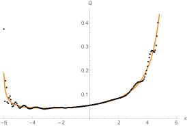
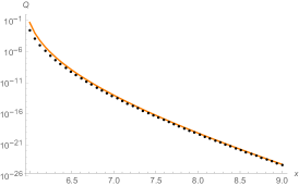
Figure 1: Normalized expected charge density in the discrete model (dots) and continuum quantum field theory (curves). Plots depict the left (dots) and the right side (curves) of (13) for mass $m=4$, lattice step $\varepsilon=0.03$, time $t=6$, and position $x$ being an even multiple of $\varepsilon$.

1 Introduction

We present a new completely elementary model which describes creation, annihilation and motion of non-interacting electrons and positrons along a line (see Definitions 2, 3, and 5). It is a modification of the model known as Feynman checkers, or one-dimensional quantum walk, or Ising model at imaginary temperature (see Definition 1 and surveys [13, 15, 24, 28]).

This modification preserves known identities (see §2.5) and Fourier integral representation (see Proposition 1) but adds antiparticles (and thus is called Feynman anticheckers). The discrete model is consistent with the continuum quantum field theory, namely, reproduces the known expected charge density as lattice step tends to zero (see Figure 1 and Corollary 1). It is exactly solvable via hypergeometric functions (see Proposition 3) and is described asymptotically by Bessel and trigonometric functions (see Theorems 2–3). We introduce interaction resembling Fermi theory and get perturbation expansion (see Definition 6 and Proposition 21).

1.1 Background

One of the main open problems in mathematics is a rigorous definition of quantum field theory. For instance, the case of $4$-dimensional Yang–Mills theory is a Millennium Problem.

A perspective approach to the problem is constructive field theory, which constructs a continuum theory as a limit of discrete ones [9]. This leads to the consistency question of whether the discrete objects indeed approximate the desired continuum ones.

Constructive field theory is actually as old as quantum field theory itself. The most elementary model of electron motion known as Feynman checkers or quantum walk was introduced by R.Feynman in 1940s and first published in 1965 [5]. Consistency with continuum quantum mechanics was posed as a problem there [5, Problem 2.6]; it was solved mathematically only recently [24]. See also surveys [13, 15, 24, 28] on Feynman’s model and its generalizations.

In 1970s F. Wegner and K. Wilson introduced lattice gauge theory as a computational tool for gauge theory describing all known interactions (except gravity); see [18] for a popular-science introduction. This theory is Euclidean in the sense that it involves imaginary time. Euclidean lattice field theory became one of the main computational tools [22] and culminated in determining the proton mass theoretically with error less than $2\%$ in a sense. There were developed methods to establish consistency, such as Reisz power counting theorem [22, §13.3]. This lead to some rigorous constructions of field theories in dimension 2 and 3 [9].

Euclidean theories are related to statistical physics via the equivalence between imaginary time and temperature [29, §V.2]. For instance, Feynman checkers can be viewed as an Ising model at imaginary temperature [24, §2.2], whereas Euclidean theory of an electron is an Ising model at real temperature. S. Smirnov and coauthors proved consistency for a wide class of $2$-dimensional models including the Ising one and some loop $O(n)$ models [26]. Euclidean theories involving electrons suffer from fermion doubling, unavoidable by the Nielsen–Ninomiya no-go theorem, and often making them inconsistent [22, §4.2].

A new promising direction is Minkowskian lattice quantum field theory, where time is real and fermion doubling is possibly avoided [8, §4.1.1] (cf. staggered fermions [22, §4.4]). Feynman checkers is a reasonable starting point. It was an old dream to incorporate creation and annihilation of electron-positron pairs in it (see [23, p. 481–483], [12]), celebrating a passage from quantum mechanics to quantum field theory (second quantization). One looked for a combinatorial model reproducing Feynman propagator (11) in the continuum limit. Known constructions (such as hopping expansion [22, §12]) did not lead to the Feynman propagator because of fermion doubling. In the massless case, a non-combinatorial construction was given by C. Bender–L. Mead–K. Milton–D. Sharp in [2, §9F] and [3, §IV].

The desired combinatorial construction is finally given in this paper (realizing two steps of the program outlined in [24, §§8–9]). It follows a classical approach known from Kirchhoff matrix-tree theorem, the Kasteleyn and Kenyon theorems [17, 14]. In this approach, a physical system (an electrical network, a moving electron, etc) is described by a difference equation on the lattice (lattice Laplace equation, lattice Dirac equation from Feynman checkers, etc). The solution is expressed through determinants, interpreted combinatorially via loop expansion [22, §12.3], and computed explicitly by Fourier transform. In our setup, the solution is not unique and has to be regularized first by introducing a small imaginary mass ‘‘living’’ on the dual lattice.

1.2 Organization of the paper

In §2 we define the new model and list its properties. In §3 we discuss its generalizations and in §4 we give proofs. In Appendices A and B we give alternative definitions/proofs and put the model in the general framework of quantum field theory respectively.

The paper assumes no background in physics. The definitions in §2–3 are completely elementary (in particular, we use neither Hilbert spaces nor Grassman variables).

The paper is written in a mathematical level of rigor, in the sense that all the definitions, conventions, and theorems (including corollaries, propositions, lemmas) should be understood literally. Theorems remain true, even if cut out from the text. The proofs of theorems use the statements but not the proofs of the other ones. Most statements are much less technical than the proofs; hence the proofs are kept in a separate section (§4) and long computations are kept in [25]. Remarks are informal and usually not used elsewhere (hence skippable). Text outside definitions, theorems, proofs is neither used formally.

2 Feynman anticheckers: statements

2.1 Construction outline

Let us recall the definition of Feynman’s original model, and then outline how it is modified.

Definition 1.

Fix $\varepsilon>0$ and $m\geq 0$ called lattice step and particle mass respectively. Consider the lattice $\varepsilon\mathbb{Z}^{2}=\{\,(x,t):x/\varepsilon,t/\varepsilon\in\mathbb{Z}\,\}$ (see Figure 2 to the left). A checker path $s$ is a finite sequence of lattice points such that the vector from each point (except the last one) to the next one equals either $(\varepsilon,\varepsilon)$ or $(-\varepsilon,\varepsilon)$. Denote by $\mathrm{turns}(s)$ the number of points in $s$ (not the first and not the last one) such that the vectors from the point to the next and to the previous ones are orthogonal. To the path $s$, assign the complex number

$$a(s):=(1+m^{2}\varepsilon^{2})^{1-n/2}\,i(-im\varepsilon)^{\mathrm{turns}(s)},$$

where $n$ is the total number of points in $s$. For each $(x,t)\in\varepsilon\mathbb{Z}^{2}$, where $t>0$, denote by

$${a}(x,t,m,\varepsilon):=\sum_{s}a(s)$$

the sum over all checker paths $s$ from $(0,0)$ to $(x,t)$ containing $(\varepsilon,\varepsilon)$. An empty sum is set to be zero by definition. Denote

$$a_{1}(x,t,m,\varepsilon):=\mathrm{Re}\,a(x,t,m,\varepsilon),\quad a_{2}(x,t,m,\varepsilon):=\mathrm{Im}\,a(x,t,m,\varepsilon).$$

Physical interpretation.

One interprets $|{a}(x,t,m,\varepsilon)|^{2}$ as the probability to find an electron of mass $m$ in the interval of length $\varepsilon$ around the point $x$ at the time $t>0$, if the electron was emitted from the origin at the time $0$. Hereafter we work in a natural system of units where $\hbar=c=e=1$ (setting all those constants to $1$ is possible for vacuum permittivity $\varepsilon_{0}\neq 1$).

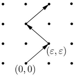
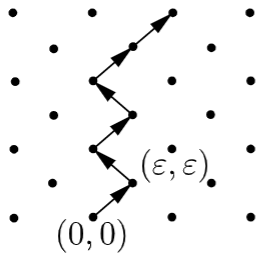
Figure 2: A checker path (left). A generalized checker path (right). See Definitions 1 and 3.

We have the following recurrence relation called lattice Dirac equation [24, Proposition 5]:

$$a_{1}(x,t,m,\varepsilon) =\frac{1}{\sqrt{1+m^{2}\varepsilon^{2}}}(a_{1}(x+\varepsilon,t-\varepsilon,m,\varepsilon)+m\varepsilon\,a_{2}(x+\varepsilon,t-\varepsilon,m,\varepsilon)),$$

$$a_{2}(x,t,m,\varepsilon) =\frac{1}{\sqrt{1+m^{2}\varepsilon^{2}}}(a_{2}(x-\varepsilon,t-\varepsilon,m,\varepsilon)-m\varepsilon\,a_{1}(x-\varepsilon,t-\varepsilon,m,\varepsilon)).$$

Informally, the new model is obtained by the following modification of lattice Dirac equation:

Step 0:

the functions $a_{1}$ and $a_{2}$ are extended to the dual lattice, shifts by $\pm\varepsilon$ are replaced by shifts by $\pm\varepsilon/2$ in their arguments, and a term vanishing outside the origin is added;

Step 1:

the particle mass acquires small imaginary part which we eventually tend to zero;

Step 2:

on the dual lattice, the mass is replaced by its imaginary part.

This makes lattice Dirac equation uniquely solvable in $L^{2}$, and the solution is much different from $(a_{1},a_{2})$: we get two complex functions rather than components of one complex function.

The elementary combinatorial definition (see Definition 3) is obtained from Feynman’s one (see Definition 1) by slightly more involved modification starting with the same Step 1:

Step 2^′:

just like the real mass is ‘‘responsible’’ for turns at the points of the lattice, the imaginary one allows turns at the points of the dual lattice (see Figure 2 to the right);

Step 3^′:

the infinite lattice is replaced by a torus with the size eventually tending to infinity;

Step 4^′:

the sum over checker paths is replaced by a ratio of sums over loop configurations.

The resulting loops are interpreted as the Dirac sea of electrons filling the whole space, and the edges not in the loops form paths of holes in the sea, that is, positrons.

In this informal outline, Steps 2 and 2^′ are completely new whereas the other ones are standard. The former reflect a general principle that the real and the imaginary part of a quantity should be always put on dual lattices. Thus in what follows we consider a new lattice which is the disjoint union of the initial lattice $\varepsilon\mathbb{Z}^{2}$ and its dual; the latter become sublattices.

2.2 Axiomatic definition

Definition 2.

Fix $\varepsilon,m,\delta>0$ called lattice step, particle mass, and small imaginary mass respectively. Assume $\delta<1$. For two elements $x,y$ of the same set denote

$$\delta_{xy}:=\begin{cases}1,&\text{for }x=y,\\ 0,&\text{for }x\neq y.\end{cases}$$

Define a pair of complex-valued functions $A_{k}(x,t)=A_{k}(x,t,m,\varepsilon,\delta)$, where $k\in\{1,2\}$, on the set $\{\,(x,t)\in\mathbb{R}^{2}:2x/\varepsilon,2t/\varepsilon,(x+t)/\varepsilon\in\mathbb{Z}\,\}$ by the following $3$ conditions:

axiom 1:

for each $(x,t)$ with $2x/\varepsilon$ and $2t/\varepsilon$ even,

$$A_{1}(x,t) =\frac{1}{\sqrt{1+m^{2}\varepsilon^{2}}}\left(A_{1}\left(x+\frac{\varepsilon}{2},t-\frac{\varepsilon}{2}\right)+m\varepsilon\,A_{2}\left(x+\frac{\varepsilon}{2},t-\frac{\varepsilon}{2}\right)\right),$$

$$A_{2}(x,t) =\frac{1}{\sqrt{1+m^{2}\varepsilon^{2}}}\left(A_{2}\left(x-\frac{\varepsilon}{2},t-\frac{\varepsilon}{2}\right)-m\varepsilon\,A_{1}\left(x-\frac{\varepsilon}{2},t-\frac{\varepsilon}{2}\right)\right)+2\delta_{x0}\delta_{t0};$$

axiom 2:

for each $(x,t)$ with $2x/\varepsilon$ and $2t/\varepsilon$ odd,

$$A_{1}(x,t) =\frac{1}{\sqrt{1-\delta^{2}}}\left(A_{1}\left(x+\frac{\varepsilon}{2},t-\frac{\varepsilon}{2}\right)-i\delta\,A_{2}\left(x+\frac{\varepsilon}{2},t-\frac{\varepsilon}{2}\right)\right),$$

$$A_{2}(x,t) =\frac{1}{\sqrt{1-\delta^{2}}}\left(A_{2}\left(x-\frac{\varepsilon}{2},t-\frac{\varepsilon}{2}\right)+i\delta\,A_{1}\left(x-\frac{\varepsilon}{2},t-\frac{\varepsilon}{2}\right)\right);$$

axiom 3:

$\sum_{(x,t)\in\varepsilon\mathbb{Z}^{2}}\left(\left|A_{1}(x,t)\right|^{2}+\left|A_{2}(x,t)\right|^{2}\right)<\infty.$

For each $k\in\{1,2\}$ and $(x,t)\in\varepsilon\mathbb{Z}^{2}$ define the lattice propagator to be the limit

$$\widetilde{A}_{k}(x,t):=\widetilde{A}_{k}(x,t,m,\varepsilon):=\lim_{\delta\searrow 0}A_{k}(x,t,m,\varepsilon,\delta).$$ (1)

Theorem 1 (Consistency of the axioms and concordance to Feynman’s model).

The functions $A_{k}(x,t,m,\varepsilon,\delta)$ and the lattice propagator $\widetilde{A}_{k}(x,t,m,\varepsilon)$ are well-defined, that is, there exists a unique pair of functions satisfying axioms 1–3, and limit (1) exists for each $(x,t)\in\varepsilon\mathbb{Z}^{2}$ and $k\in\{1,2\}$. For $(x+t)/\varepsilon+k$ even, the limit is real and given by

$$\widetilde{A}_{1}(x,t,m,\varepsilon) =a_{1}(x,|t|+\varepsilon,m,\varepsilon), (x+t)/\varepsilon$$ for odd,

$$\widetilde{A}_{2}(x,t,m,\varepsilon) =\pm a_{2}(\pm x+\varepsilon,|t|+\varepsilon,m,\varepsilon), (x+t)/\varepsilon$$ for even,

where the minus signs are taken when $t<0$. For $(x+t)/\varepsilon+k$ odd, limit (1) is purely imaginary.

Once again we see that the real and imaginary parts live on dual sublattices.

Physical interpretation.

One interprets

$$Q\left(x,t,m,\varepsilon\right):=\frac{1}{2}\left|\widetilde{A}_{1}\left(x,t,m,\varepsilon\right)\right|^{2}+\frac{1}{2}\left|\widetilde{A}_{2}\left(x,t,m,\varepsilon\right)\right|^{2}$$ (2)

as the expected charge in the interval of length $\varepsilon$ around the point $x$ at the time $t>0$, if an electron of mass $m$ was emitted from the origin at the time $0$ (or a positron is absorbed there). Unlike the original Feynman checkers, this value cannot be interpreted as probability [24, §9.2]: virtual electrons and positrons also contribute to the charge.

2.3 Exact solution

Now we state a result which reduces investigation of the new model to analysis of certain integral. One can use it as an alternative definition of the model. The integral coincides with the one arising in the original Feynman’s model [24, Proposition 12] but now is computed for arbitrary parity of $(x+t)/\varepsilon$.

Proposition 1 (Fourier integral).

For each $m,\varepsilon>0$ and $(x,t)\in\varepsilon\mathbb{Z}^{2}$ we have

$$\widetilde{A}_{1}(x,t,m,\varepsilon) =\pm\frac{im\varepsilon^{2}}{2\pi}\int_{-\pi/\varepsilon}^{\pi/\varepsilon}\frac{e^{ipx-i\omega_{p}t}\,dp}{\sqrt{m^{2}\varepsilon^{2}+\sin^{2}(p\varepsilon)}};$$

$$\widetilde{A}_{2}(x,t,m,\varepsilon) =\pm\frac{\varepsilon}{2\pi}\int_{-\pi/\varepsilon}^{\pi/\varepsilon}\left(1+\frac{\sin(p\varepsilon)}{\sqrt{m^{2}\varepsilon^{2}+\sin^{2}(p\varepsilon)}}\right)e^{ipx-i\omega_{p}t}\,dp,$$

where the minus sign in the expression for $\widetilde{A}_{k}$ is taken for $t<0$ and $(x+t)/\varepsilon+k$ even, and

$$\omega_{p}:=\frac{1}{\varepsilon}\arccos\left(\frac{\cos p\varepsilon}{\sqrt{1+m^{2}\varepsilon^{2}}}\right).$$ (3)

Physical interpretation.

Fourier integral represents a wave emitted by a point source as a superposition of waves of wavelength $2\pi/p$ and frequency $\omega_{p}$. Plank and de Broglie relations assert that $\omega_{p}$ and $p$ are the energy and the momentum of the waves. As $\varepsilon\to 0$, the energy $\omega_{p}$ tends to the expression $\sqrt{m^{2}+p^{2}}$ (see Lemma 4). The latter expression is standard; it generalizes Einstein formula $\hbar\omega_{0}=mc^{2}$ relating particle energy and mass (recall that $\hbar=c=1$ in our units). Fourier integral resembles the spin-$1/2$ Feynman propagator describing creation, annihilation and motion of non-interacting electrons and positrons along a line in quantum field theory [7, (6.45),(6.50)–(6.51)]:

$$G^{F}(x,t,m)=\frac{1}{4\pi}\int_{-\infty}^{+\infty}\begin{pmatrix}\frac{im}{\sqrt{m^{2}+p^{2}}}&1+\frac{p}{\sqrt{m^{2}+p^{2}}}\\ -1+\frac{p}{\sqrt{m^{2}+p^{2}}}&\frac{im}{\sqrt{m^{2}+p^{2}}}\end{pmatrix}e^{ipx-i\sqrt{m^{2}+p^{2}}t}\,dp\qquad\text{for }t>0.$$ (4)

Here the integral is understood as Fourier transform of matrix-valued tempered distributions. (We do not use (4) in this paper and hence do not define those notions. Cf. (11))

Example 1 (Massless and heavy particles).

(Cf. [3]) For each $(x,t)\in\varepsilon\mathbb{Z}^{2}$ we have

$$\widetilde{A}_{k}(x,t,\infty,\varepsilon) :=\lim_{m\to+\infty}\widetilde{A}_{k}(x,t,m,\varepsilon)=\delta_{x0}(-i)^{|t/\varepsilon+k-1|-1},$$

$$\widetilde{A}_{1}(x,t,0,\varepsilon) :=\lim_{m\searrow 0}\widetilde{A}_{1}(x,t,m,\varepsilon)=0,$$

$$\widetilde{A}_{2}(x,t,0,\varepsilon) :=\lim_{m\searrow 0}\widetilde{A}_{2}(x,t,m,\varepsilon)=\begin{cases}1,&\text{for }x=t\geq 0,\\ -1,&\text{for }x=t<0,\\ {2i\varepsilon}/{\pi(x-t)},&\text{for }{(x+t)}/{\varepsilon}\text{ odd},\\ 0,&\text{otherwise.}\end{cases}$$ (5)

Physically this means that an infinitely heavy particle stays at the origin forever, and a massless particle forms a charged ‘‘cloud’’ moving with the speed of light. The massless lattice propagator is proportional to the massless spin-$1/2$ Feynman propagator defined by

$$G^{F}(x,t,0):=\left(\begin{smallmatrix}0&i/2\pi(x-t)\\ i/2\pi(x+t)&0\end{smallmatrix}\right)\qquad\text{for }|x|\neq|t|.$$ (6)

Example 2 (Unit mass and lattice step).

The value

$$\widetilde{A}_{1}(0,0,1,1)/i =\Gamma(\tfrac{1}{4})^{2}/(2\pi)^{3/2}=\tfrac{2}{\pi}K(i)=:G\approx 0.83463$$ (7)

is the Gauss constant and

$$\widetilde{A}_{2}(1,0,1,1)/i =2\sqrt{2\pi}/\Gamma(\tfrac{1}{4})^{2}=\tfrac{2}{\pi}(E(i)-K(i))=1/\pi G=:L^{\prime}\approx 0.38138$$ (8)

is the inverse lemniscate constant (cf. [6, §6.1]), where $K(z):=\int_{0}^{\pi/2}d\theta/\sqrt{1-z^{2}\sin^{2}\theta}$ and $E(z):=\int_{0}^{\pi/2}\sqrt{1-z^{2}\sin^{2}\theta}\,d\theta$ are the complete elliptic integrals of the 1st and 2nd kind respectively. The other values are even more complicated irrationalities (see Table 1).

Proposition 2 (Rational basis).

For each $k\in\{1,2\}$ and $(x,t)\in\mathbb{Z}^{2}$ the values $2^{|t|/2}\mathrm{Re}\,\widetilde{A}_{k}(x,t,1,1)$ are integers and $2^{|t|/2}\mathrm{Im}\,\widetilde{A}_{k}(x,t,1,1)$ are rational linear combinations of numbers (7) and (8).

$\widetilde{A}_{1}(x,t,1,1)$
$2$ $0$ ${i\frac{2G-3L^{\prime}}{3}}$ $\frac{1}{2}$ ${-iL^{\prime}}$ $\frac{1}{2}$ ${i\frac{2G-3L^{\prime}}{3}}$ $0$ $1$ ${i\frac{7G-15L^{\prime}}{3\sqrt{2}}}$ $0$ ${i\frac{G-L^{\prime}}{\sqrt{2}}}$ $\frac{1}{\sqrt{2}}$ ${i\frac{G-L^{\prime}}{\sqrt{2}}}$ $0$ ${i\frac{7G-15L^{\prime}}{3\sqrt{2}}}$ $0$ $0$ ${i(G-2L^{\prime})}$ $0$ ${iG}$ $0$ ${i(G-2L^{\prime})}$ $0$ $-1$ ${i\frac{7G-15L^{\prime}}{3\sqrt{2}}}$ $0$ ${i\frac{G-L^{\prime}}{\sqrt{2}}}$ $\frac{1}{\sqrt{2}}$ ${i\frac{G-L^{\prime}}{\sqrt{2}}}$ $0$ ${i\frac{7G-15L^{\prime}}{3\sqrt{2}}}$ $-2$ $0$ ${i\frac{2G-3L^{\prime}}{3}}$ $\frac{1}{2}$ ${-iL^{\prime}}$ $\frac{1}{2}$ ${i\frac{2G-3L^{\prime}}{3}}$ $0$ $-3$ $-2$ $-1$ $0$ $1$ $2$ $3$
$\widetilde{A}_{2}(x,t,1,1)$
$2$ $i\frac{5G-12L^{\prime}}{15}$ $0$ $-i\frac{G}{3}$ $-\frac{1}{2}$ $-iG$ $\frac{1}{2}$ $i\frac{-5G+12L^{\prime}}{3}$ $1$ $0$ $i\frac{G-3L^{\prime}}{3\sqrt{2}}$ $0$ $-i\frac{G+L^{\prime}}{\sqrt{2}}$ $\frac{1}{\sqrt{2}}$ $i\frac{-G+3L^{\prime}}{\sqrt{2}}$ $0$ $0$ $i\frac{4G-9L^{\prime}}{3}$ $0$ $-iL^{\prime}$ $1$ $iL^{\prime}$ $0$ $i\frac{-4G+9L^{\prime}}{3}$ $-1$ $0$ $i\frac{G-3L^{\prime}}{\sqrt{2}}$ $-\frac{1}{\sqrt{2}}$ $i\frac{G+L^{\prime}}{\sqrt{2}}$ $0$ $i\frac{-G+3L^{\prime}}{3\sqrt{2}}$ $0$ $-2$ $i\frac{5G-12L^{\prime}}{3}$ $-\frac{1}{2}$ $iG$ $\frac{1}{2}$ $i\frac{G}{3}$ $0$ $i\frac{-5G+12L^{\prime}}{15}$ $-3$ $-2$ $-1$ $0$ $1$ $2$ $3$

Table 1: The values $\widetilde{A}_{1}(x,t,1,1)$ and $\widetilde{A}_{2}(x,t,1,1)$ for small $x,t$ (see Definition 3 and Example 2)

In general, the propagator is ‘‘explicitly’’ expressed through the Gauss hypergeometric function. Denote by ${}_{2}F_{1}(p,q;r;z)$ the principal branch of the function defined by [10, 9.111].

Proposition 3.

(‘‘Explicit’’ formula) For each $m,\varepsilon>0$ and $(x,t)\in\varepsilon\mathbb{Z}^{2}$ we have

$$\widetilde{A}_{1}(x,t,m,\varepsilon) =\pm i\frac{(-im\varepsilon)^{\frac{t-|x|}{\varepsilon}}}{\left({1+m^{2}\varepsilon^{2}}\right)^{\frac{t}{2\varepsilon}}}\binom{\frac{t+|x|}{2\varepsilon}-\frac{1}{2}}{|x|/\varepsilon}{}_{2}F_{1}\left(\frac{1}{2}+\frac{|x|-t}{2\varepsilon},\frac{1}{2}+\frac{|x|-t}{2\varepsilon};1+\frac{|x|}{\varepsilon};-\frac{1}{m^{2}\varepsilon^{2}}\right),$$

$$\widetilde{A}_{2}(x,t,m,\varepsilon) =\pm\frac{(-im\varepsilon)^{\frac{t-|x|}{\varepsilon}}}{\left({1+m^{2}\varepsilon^{2}}\right)^{\frac{t}{2\varepsilon}}}\binom{\frac{t+|x|}{2\varepsilon}-1+\theta(x)}{|x|/\varepsilon}{}_{2}F_{1}\left(\frac{|x|-t}{2\varepsilon},1+\frac{|x|-t}{2\varepsilon};1+\frac{|x|}{\varepsilon};-\frac{1}{m^{2}\varepsilon^{2}}\right),$$

where the minus sign in the expression for $\widetilde{A}_{k}$ is taken for $t<0$ and $(x+t)/\varepsilon+k$ even, and

$$\theta(x) :=\begin{cases}1,&\mbox{if }x\geq 0,\\ 0,&\mbox{if }x<0;\end{cases} \binom{z}{n} :=\frac{1}{n!}\prod_{j=1}^{n}(z-j+1).$$

Remark 1.

Depending on the parity of $(x+t)/\varepsilon$, those expressions can be rewritten as Jacobi polynomials (see [24, Remark 3]) or as Jacobi functions of the 2nd kind of half-integer order (see the definition in [27, (4.61.1)]). For instance, for each $(x,t)\in\varepsilon\mathbb{Z}^{2}$ such that $|x|>t$ and $(x+t)/\varepsilon$ is even we have

$$\widetilde{A}_{1}(x,t,m,\varepsilon)=\frac{2m\varepsilon}{\pi}\left({1+m^{2}\varepsilon^{2}}\right)^{t/2\varepsilon}Q_{(|x|-t-\varepsilon)/2\varepsilon}^{(0,t/\varepsilon)}(1+2m^{2}\varepsilon^{2}).$$

Remark 2.

For even $x/\varepsilon$, the value $\widetilde{A}_{1}(x,0,m,\varepsilon)$ equals $i(1+\sqrt{1+m^{2}\varepsilon^{2}})/m\varepsilon$ times the probability that a planar simple random walk over the sublattice $\{(x,t)\in\varepsilon\mathbb{Z}^{2}:(x+t)/\varepsilon\text{ even}\}$ dies at $(x,0)$, if it starts at $(0,0)$ and dies with the probability $1-1/\sqrt{1+m^{2}\varepsilon^{2}}$ before each step. Nothing like that is known for $t\neq 0$.

2.4 Asymptotic formulae

The main result of this work is consistency of the model with continuum quantum field theory, that is, the convergence of the lattice propagator to the continuum one as the lattice becomes finer and finer (see Figure 3 and Theorem 2). More precisely, the former propagator converges to the real part of the latter on certain sublattice, and it converges to the imaginary part on the dual sublattice. The limit involves Bessel functions $J_{n}(z)$ and $Y_{n}(z)$ of the 1st and 2nd kind respectively, and modified Bessel functions $K_{n}(z)$ of the 2nd kind defined in [10, §8.40].

Theorem 2 (Asymptotic formula in the continuum limit).

For each $m,\varepsilon>0$ and $(x,t)\in\varepsilon\mathbb{Z}^{2}$ such that $|x|\neq|t|$ we have

$$\widetilde{A}_{1}\left(x,t,{m},{\varepsilon}\right) =\begin{cases}m\varepsilon\left(J_{0}(ms)+O\left(\varepsilon\Delta\right)\right),&\text{for }|x|<|t|\text{ and }(x+t)/\varepsilon\text{ odd};\\ -im\varepsilon\left(Y_{0}(ms)+O\left(\varepsilon\Delta\right)\right),&\text{for }|x|<|t|\text{ and }(x+t)/\varepsilon\text{ even};\\ 0,&\text{for }|x|>|t|\text{ and }(x+t)/\varepsilon\text{ odd};\\ \mathrlap{2im\varepsilon\left(K_{0}(ms)+O\left(\varepsilon\Delta\right)\right)/{\pi},}\hphantom{2im\varepsilon(t+x)\left(K_{1}(ms)+O\left(\varepsilon\Delta\right)\right)/\pi s,}&\text{for }|x|>|t|\text{ and }(x+t)/\varepsilon\text{ even};\end{cases}$$ (9)

$$\widetilde{A}_{2}\left(x,t,{m},{\varepsilon}\right) =\begin{cases}-m\varepsilon(t+x)\left(J_{1}(ms)+O\left(\varepsilon\Delta\right)\right)/{s},&\text{for }|x|<|t|\text{ and }(x+t)/\varepsilon\text{ even};\\ im\varepsilon(t+x)\left(Y_{1}(ms)+O\left(\varepsilon\Delta\right)\right)/{s},&\text{for }|x|<|t|\text{ and }(x+t)/\varepsilon\text{ odd};\\ 0,&\text{for }|x|>|t|\text{ and }(x+t)/\varepsilon\text{ even};\\ 2im\varepsilon(t+x)\left(K_{1}(ms)+O\left(\varepsilon\Delta\right)\right)/\pi s,&\text{for }|x|>|t|\text{ and }(x+t)/\varepsilon\text{ odd}.\end{cases}$$ (10)

$$\text{where}\qquad s:=\sqrt{\left|t^{2}-x^{2}\right|}\qquad\text{and}\qquad\Delta:=\frac{1}{\left|\,|x|-|t|\,\right|}+m^{2}(|x|+|t|).$$

Recall that $f(x,t,{m},{\varepsilon})=g(x,t,{m},{\varepsilon})+{O}\left(h(x,t,{m},{\varepsilon})\right)$ means that there is a constant $C$ (not depending on $x,t,{m},{\varepsilon}$) such that for each $x,t,{m},{\varepsilon}$ satisfying the assumptions of the theorem we have $|f(x,t,{m},{\varepsilon})-g(x,t,{m},{\varepsilon})|\leq C\,h(x,t,{m},{\varepsilon})$.

Physical interpretation.

The theorem means that in the continuum limit, the model reproduces the spin-$1/2$ Feynman propagator (cf. (4))

$$G^{F}(x,t,m):=\begin{cases}\dfrac{m}{4}\,\begin{pmatrix}J_{0}(ms)-iY_{0}(ms)&-{\frac{t+x}{s}}\left(J_{1}(ms)-iY_{1}(ms)\right)\\ {\frac{t-x}{s}}\left(J_{1}(ms)-iY_{1}(ms)\right)&J_{0}(ms)-iY_{0}(ms)\end{pmatrix},&\text{if }|x|<|t|;\\ \dfrac{im}{2\pi}\,\begin{pmatrix}K_{0}(ms)&{\frac{t+x}{s}}\,K_{1}(ms)\\ {\frac{x-t}{s}}\,K_{1}(ms)&K_{0}(ms)\end{pmatrix},&\text{if }|x|>|t|,\end{cases}$$ (11)

where again $s:=\sqrt{\left|t^{2}-x^{2}\right|}$. (A common definition involves also a generalized function supported on the lines $t=\pm x$ which we drop because those lines are excluded anyway.) The value $|G_{11}^{F}(x,t,m)|^{2}+|G_{12}^{F}(x,t,m)|^{2}$ is the expected charge density at the point $x$ at the moment $t$. Recall that Feynman’s original model reproduces just retarded propagator [24, Theorem 5].

The asymptotic formulae in Theorem 2 were known earlier (with a slightly weaker error estimates) on the sublattice, where the new model coincides with Feynman’s original one [24, Theorem 5]. Extension to the dual sublattice has required different methods.

In the following corollary, we approximate a point $(x,t)\in\mathbb{R}^{2}$ by the lattice point

$$(x_{\varepsilon},t_{\varepsilon}):=\left(2\varepsilon\!\left\lceil\frac{x}{2\varepsilon}\right\rceil,2\varepsilon\!\left\lceil\frac{t}{2\varepsilon}\right\rceil\right).$$ (12)

Corollary 1 (Uniform continuum limit; see Figures 1 and 3).

For each fixed $m\geq 0$ we have

$$\begin{aligned} \frac{1}{4\varepsilon}\,\tilde{A}_{1}\left(x_{\varepsilon}+\varepsilon,t_{\varepsilon},{m},{\varepsilon}\right)&\rightrightarrows\mathrm{Re}\,G^{F}_{11}(x,t,m);&\frac{1}{4\varepsilon}\,\tilde{A}_{1}\left(x_{\varepsilon},t_{\varepsilon},{m},{\varepsilon}\right)&\rightrightarrows i\mathrm{Im}\,G^{F}_{11}(x,t,m);\\ \frac{1}{4\varepsilon}\,\tilde{A}_{2}\left(x_{\varepsilon}+\varepsilon,t_{\varepsilon},{m},{\varepsilon}\right)&\rightrightarrows i\mathrm{Im}\,G^{F}_{12}(x,t,m);&\frac{1}{4\varepsilon}\,\tilde{A}_{2}\left(x_{\varepsilon},t_{\varepsilon},{m},{\varepsilon}\right)&\rightrightarrows\mathrm{Re}\,G^{F}_{12}(x,t,m);\end{aligned}$$

$$\frac{1}{8\varepsilon^{2}}\,\left(Q\left(x_{\varepsilon},t_{\varepsilon},{m},{\varepsilon}\right)+Q\left(x_{\varepsilon}+\varepsilon,t_{\varepsilon},{m},{\varepsilon}\right)\right)\rightrightarrows|G^{F}_{11}(x,t,m)|^{2}+|G^{F}_{12}(x,t,m)|^{2}$$ (13)

as $\varepsilon\to 0$ uniformly on compact subsets of $\mathbb{R}^{2}\setminus\{|t|=|x|\}$, under notation (12),(11),(2),(5),(6).

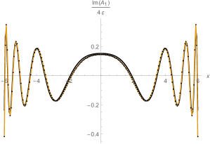
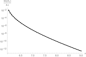
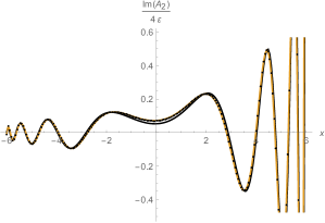
Figure 3: Plots of (the normalized imaginary part of) the lattice propagators $\mathrm{Im}\,\widetilde{A}_{1}(x,6,4,0.03)/0.12$ (top, dots) and $\mathrm{Im}\,\widetilde{A}_{2}(x,6,4,0.03)/0.12$ (bottom, dots) for $x/0.06\in\mathbb{Z}$ and $x/0.06+1/2\in\mathbb{Z}$ respectively, their analytic approximations from Theorems 2 (dark curve) and 3 (light curve). The former approximation is the imaginary part of the spin-$1/2$ Feynman propagator $\mathrm{Im}\,G^{F}_{11}(x,6,4)$ (top, dark) and $\mathrm{Im}\,G^{F}_{12}(x,6,4)$ (bottom, dark) given by (11).

The following result follows from Proposition 1 and [24, Theorems 2 and 7]; cf. [20].

Theorem 3 (Large-time asymptotic formula between the peaks; see Figure 3).

For each $\Delta>0$ there is $C_{\Delta}>0$ such that for each $m,\varepsilon>0$ and each $(x,t)\in\varepsilon\mathbb{Z}^{2}$ satisfying

$$|x|/t<1/\sqrt{1+m^{2}\varepsilon^{2}}-\Delta,\qquad\varepsilon\leq 1/m,\qquad t>C_{\Delta}/m,$$ (14)

we have

$$\widetilde{A}_{1}\left(x,t,m,\varepsilon\right) =\begin{cases}{\varepsilon}\sqrt{\frac{2m}{\pi}}\frac{\sin(\theta(x,t,m,\varepsilon)+\pi/4)}{\left(t^{2}-(1+m^{2}\varepsilon^{2})x^{2}\right)^{1/4}}+O_{\Delta}\left(\frac{\varepsilon}{m^{1/2}t^{3/2}}\right),&\text{for }(x+t)/\varepsilon\text{ odd};\\ \mathrlap{i{\varepsilon}\sqrt{\frac{2m}{\pi}}\frac{\cos(\theta(x,t,m,\varepsilon)+\pi/4)}{\left(t^{2}-(1+m^{2}\varepsilon^{2})x^{2}\right)^{1/4}}+O_{\Delta}\left(\frac{\varepsilon}{m^{1/2}t^{3/2}}\right),}\hphantom{-i{\varepsilon}\sqrt{\frac{2m}{\pi}}\sqrt{\frac{t+x}{t-x}}\frac{\sin(\theta(x,t,m,\varepsilon)+\pi/4)}{\left(t^{2}-(1+m^{2}\varepsilon^{2})x^{2}\right)^{1/4}}+O_{\Delta}\left(\frac{\varepsilon}{m^{1/2}t^{3/2}}\right),}&\text{for }(x+t)/\varepsilon\text{ even};\end{cases}$$

$$\widetilde{A}_{2}\left(x,t,m,\varepsilon\right) =\begin{cases}{\varepsilon}\sqrt{\frac{2m}{\pi}}\sqrt{\frac{t+x}{t-x}}\frac{\cos(\theta(x,t,m,\varepsilon)+\pi/4)}{\left(t^{2}-(1+m^{2}\varepsilon^{2})x^{2}\right)^{1/4}}+O_{\Delta}\left(\frac{\varepsilon}{m^{1/2}t^{3/2}}\right),&\text{for }(x+t)/\varepsilon\text{ even};\\ -i{\varepsilon}\sqrt{\frac{2m}{\pi}}\sqrt{\frac{t+x}{t-x}}\frac{\sin(\theta(x,t,m,\varepsilon)+\pi/4)}{\left(t^{2}-(1+m^{2}\varepsilon^{2})x^{2}\right)^{1/4}}+O_{\Delta}\left(\frac{\varepsilon}{m^{1/2}t^{3/2}}\right),&\text{for }(x+t)/\varepsilon\text{ odd},\end{cases}$$

where

$$\theta(x,t,m,\varepsilon) :=\frac{t}{\varepsilon}\arcsin\frac{m\varepsilon t}{\sqrt{\left(1+m^{2}\varepsilon^{2}\right)\left(t^{2}-x^{2}\right)}}-\frac{x}{\varepsilon}\arcsin\frac{m\varepsilon x}{\sqrt{t^{2}-x^{2}}}.$$

Here the notation $f(x,t,m,\varepsilon)=g(x,t,m,\varepsilon)+{O}_{\Delta}\left(h(x,t,m,\varepsilon)\right)$ means that there is a constant $C(\Delta)$ (depending on $\Delta$ but not on $x,t,m,\varepsilon$) such that for each $x,t,m,\varepsilon$ satisfying the assumptions of the theorem we have $|f(x,t,m,\varepsilon)-g(x,t,m,\varepsilon)|\leq C(\Delta)\,h(x,t,m,\varepsilon)$.

Physical interpretation.

Here $-\theta(x,t,m,\varepsilon)$ has the meaning of action. As $\varepsilon\to 0$, it tends to the action $-m\sqrt{t^{2}-x^{2}}$ of free relativistic particle (moving from the origin to $(x,t)$ with constant speed). If we introduce the Lagrangian $\mathcal{L}(v):=-\theta(vt,t,m,\varepsilon)/t$, then the well-known relation between energy (3), momentum $p$, and Lagrangian $\mathcal{L}$ holds: $\omega_{p}=pv-\mathcal{L}$ for $p=\partial\mathcal{L}/\partial v$.

2.5 Identities

Now we establish the following informal assertion (see Propositions 4–11 for formal ones).

Consistency Principle.

The new model satisfies the same identities as Feynman’s one.

In particular, the identities in this subsection are known (and easy to deduce from Definition 1) for the sublattice, where the new model coincides with the original one [24, Propositions 5–10]. For the dual sublattice, these results are not so easy to prove. Further, for the former sublattice, there are a few ‘‘exceptions’’ to the identities; but on the dual lattice, the imaginary part $b_{k}(x,t,m,\varepsilon)$ defined in [24, Definition 5] satisfies known identities [24, Propositions 5–8 and 10] literally for both $t>0$ and $t\leq 0$.

In what follows we fix $m,\varepsilon>0$ and omit the arguments $m,\varepsilon$ of the propagators.

Proposition 4 (Dirac equation).

For each $(x,t)\in\varepsilon\mathbb{Z}^{2}$ we have

$$\tilde{A}_{1}(x,t) =\frac{1}{\sqrt{1+m^{2}\varepsilon^{2}}}(\tilde{A}_{1}(x+\varepsilon,t-\varepsilon)+m\varepsilon\,\tilde{A}_{2}(x,t-\varepsilon)),$$ (15)

$$\tilde{A}_{2}(x,t) =\frac{1}{\sqrt{1+m^{2}\varepsilon^{2}}}(\tilde{A}_{2}(x-\varepsilon,t-\varepsilon)-m\varepsilon\,\tilde{A}_{1}(x,t-\varepsilon))+2\delta_{x0}\delta_{t0}.$$ (16)

In the limit $\varepsilon\to 0$, this reproduces the Dirac equation in $1$ space- and $1$ time-dimension

$$\begin{pmatrix}m&\partial/\partial x-\partial/\partial t\\ \partial/\partial x+\partial/\partial t&m\end{pmatrix}\begin{pmatrix}G^{F}_{12}(x,t)\\ G^{F}_{11}(x,t)\end{pmatrix}=\begin{pmatrix}0\\ \delta(x)\delta(t)\end{pmatrix}.$$

Proposition 5 (Klein–Gordon equation).

For each $k\in\{1,2\}$ and each $(x,t)\in\varepsilon\mathbb{Z}^{2}$, where $(x,t)\neq(0,0)$ for $k=1$ and $(x,t)\neq(-\varepsilon,0),(0,-\varepsilon)$ for $k=2$, we have

$$\sqrt{1+m^{2}\varepsilon^{2}}\,\widetilde{A}_{k}(x,t+\varepsilon)+\sqrt{1+m^{2}\varepsilon^{2}}\,\widetilde{A}_{k}(x,t-\varepsilon)-\widetilde{A}_{k}(x+\varepsilon,t)-\widetilde{A}_{k}(x-\varepsilon,t)=0.$$

In the limit $\varepsilon\to 0$, this gives the Klein–Gordon equation $\left(\tfrac{\partial^{2}}{\partial t^{2}}-\tfrac{\partial^{2}}{\partial x^{2}}+m^{2}\right)G^{F}_{1k}(x,t)=0$.

The infinite-lattice propagator has the same reflection symmetries as the continuum one.

Proposition 6 (Skew-symmetry).

For each $(x,t)\in\varepsilon\mathbb{Z}^{2}$, where $(x,t)\neq(0,0)$, we have

$$\widetilde{A}_{1}(x,t)=\widetilde{A}_{1}(-x,t)=\widetilde{A}_{1}(x,-t)=\widetilde{A}_{1}(-x,-t),$$

$$\widetilde{A}_{2}(x,t)=-\widetilde{A}_{2}(-x,-t),\qquad\qquad(t-x)\,\widetilde{A}_{2}(x,t)=(t+x)\,\widetilde{A}_{2}(-x,t).$$

Proposition 7 (Charge conservation).

For each $t\in\varepsilon\mathbb{Z}$, $\sum\limits_{x\in\varepsilon\mathbb{Z}}\dfrac{|\widetilde{A}_{1}\left(x,t\right)|^{2}+|\widetilde{A}_{2}\left(x,t\right)|^{2}}{2}=1$.

There are two versions of Huygens’ principle (cf. [24, Proposition 9]).

Proposition 8 (Huygens’ principle).

For each $x,t,t^{\prime}\in\varepsilon\mathbb{Z}$, where $t\geq t^{\prime}\geq 0$, we have

$$\widetilde{A}_{1}(x,t) =\frac{1}{2}\sum\limits_{\begin{subarray}{c}x^{\prime}\in\varepsilon\mathbb{Z}\end{subarray}}\left(\widetilde{A}_{2}(x^{\prime},t^{\prime})\widetilde{A}_{1}(x-x^{\prime},t-t^{\prime})+\widetilde{A}_{1}(x^{\prime},t^{\prime})\widetilde{A}_{2}(x^{\prime}-x,t-t^{\prime})\right),$$

$$\widetilde{A}_{2}(x,t) =\frac{1}{2}\sum\limits_{\begin{subarray}{c}x^{\prime}\in\varepsilon\mathbb{Z}\end{subarray}}\left(\widetilde{A}_{2}(x^{\prime},t^{\prime})\widetilde{A}_{2}(x-x^{\prime},t-t^{\prime})-\widetilde{A}_{1}(x^{\prime},t^{\prime})\widetilde{A}_{1}(x^{\prime}-x,t-t^{\prime})\right).$$

In the following version of Huygens’ principle, the sums are actually finite.

Proposition 9 (Huygens’ principle).

For each $x,t,t^{\prime}\in\varepsilon\mathbb{Z}$, where $t\geq t^{\prime}\geq 0$, we have

$$\widetilde{A}_{1}(x,t) =\sum\limits_{\begin{subarray}{c}x^{\prime}\in\varepsilon\mathbb{Z}:\\ (x+x^{\prime}+t+t^{\prime})/\varepsilon\text{ odd}\end{subarray}}\widetilde{A}_{2}(x^{\prime},t^{\prime})\widetilde{A}_{1}(x-x^{\prime},t-t^{\prime})+\sum\limits_{\begin{subarray}{c}x^{\prime}\in\varepsilon\mathbb{Z}:\\ (x+x^{\prime}+t+t^{\prime})/\varepsilon\text{ even}\end{subarray}}\widetilde{A}_{1}(x^{\prime},t^{\prime})\widetilde{A}_{2}(x^{\prime}-x,t-t^{\prime}),$$

$$\widetilde{A}_{2}(x,t) =\sum\limits_{\begin{subarray}{c}x^{\prime}\in\varepsilon\mathbb{Z}:\\ (x+x^{\prime}+t+t^{\prime})/\varepsilon\text{ even}\end{subarray}}\widetilde{A}_{2}(x^{\prime},t^{\prime})\widetilde{A}_{2}(x-x^{\prime},t-t^{\prime})-\sum\limits_{\begin{subarray}{c}x^{\prime}\in\varepsilon\mathbb{Z}:\\ (x+x^{\prime}+t+t^{\prime})/\varepsilon\text{ odd}\end{subarray}}\widetilde{A}_{1}(x^{\prime},t^{\prime})\widetilde{A}_{1}(x^{\prime}-x,t-t^{\prime}).$$

Proposition 10 (Equal-time mixed recurrence).

For each $(x,t)\in\varepsilon\mathbb{Z}^{2}$ we have

$$2m\varepsilon x\widetilde{A}_{1}(x,t) =(x-t-\varepsilon)\widetilde{A}_{2}(x-\varepsilon,t)-(x-t+\varepsilon)\widetilde{A}_{2}(x+\varepsilon,t),$$ (17)

$$2m\varepsilon x\widetilde{A}_{2}(x,t) =(x+t)\widetilde{A}_{1}(x-\varepsilon,t)-(x+t)\widetilde{A}_{1}(x+\varepsilon,t).$$ (18)

In particular, $\widetilde{A}_{2}(x,0)=\left(\widetilde{A}_{1}(x-\varepsilon,0)-\widetilde{A}_{1}(x+\varepsilon,0)\right)/2m\varepsilon$ for $x\neq 0$.

Proposition 11 (Equal-time recurrence relation).

For each $(x,t)\in\varepsilon\mathbb{Z}^{2}$ we have

$$(x+\varepsilon)((x-\varepsilon)^{2}-t^{2})\widetilde{A}_{1}(x-2\varepsilon,t)+(x-\varepsilon)((x+\varepsilon)^{2}-t^{2})\widetilde{A}_{1}(x+2\varepsilon,t)=\\ =2x\left((1+2m^{2}\varepsilon^{2})(x^{2}-\varepsilon^{2})-t^{2}\right)\widetilde{A}_{1}(x,t),$$

$$(x+\varepsilon)((x-\varepsilon)^{2}-(t+\varepsilon)^{2})\widetilde{A}_{2}(x-2\varepsilon,t)+(x-\varepsilon)((x+\varepsilon)^{2}-(t-\varepsilon)^{2})\widetilde{A}_{2}(x+2\varepsilon,t)=\\ =2x\left((1+2m^{2}\varepsilon^{2})(x^{2}-\varepsilon^{2})-t^{2}+\varepsilon^{2}\right)\widetilde{A}_{2}(x,t).$$

Analogous identities can be written for any $3$ neighboring lattice points by means of Proposition 3 and Gauss contiguous relations [10, 9.137].

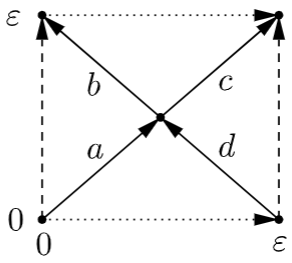
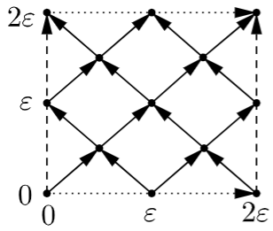
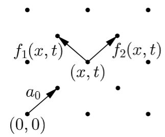
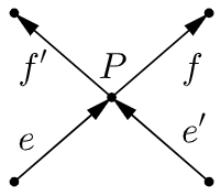
Figure 4: Lattices of sizes $1$ and $2$ (left); see Example 3. Notation for edges (right).

2.6 Combinatorial definition

Now we realize the plan from the end of §2.1, but switch the role of the lattice and its dual.

Definition 3.

Fix $T\in\mathbb{Z}$ and $\varepsilon,m,\delta>0$ called lattice size, lattice step, particle mass, and small imaginary mass respectively. Assume $T>0$ and $\delta<1$. The lattice is the quotient set

$$\faktor{\{\,(x,t)\in[0,T\varepsilon]^{2}:2x/\varepsilon,2t/\varepsilon,(x+t)/\varepsilon\in\mathbb{Z}\,\}}{\forall x,t:(x,0)\sim(x,T\varepsilon)\,\&\,(0,t)\sim(T\varepsilon,t).}$$

(This is a finite subset of the torus obtained from the square $[0,T\varepsilon]^{2}$ by an identification of the opposite sides; see Figure 4 to the left.) A lattice point $(x,t)$ is even (respectively, odd), if $2x/\varepsilon$ is even (respectively, odd). An edge is a vector starting from a lattice point $(x,t)$ and ending at the lattice point $(x+\varepsilon/2,t+\varepsilon/2)$ or $(x-\varepsilon/2,t+\varepsilon/2)$.

A generalized checker path (or just a path) is a finite sequence of distinct edges such that the endpoint of each edge is the starting point of the next one. A cycle is defined analogously, only the sequence has the unique repetition: the first and the last edges coincide, and there is at least one edge in between. (In particular, a path such that the endpoint of the last edge is the starting point of the first one is not yet a cycle; coincidence of the first and the last edges is required. The first and the last edges of a path coincide only if the path has a single edge. Thus in our setup, a path is never a cycle.) Changing the starting edge of a cycle means removal of the first edge from the sequence, then a cyclic permutation, and then adding the last edge of the resulting sequence at the beginning. A loop is a cycle up to changing of the starting edge.

A node of a path or loop $s$ is an ordered pair of consecutive edges in $s$ (the order of the edges in the pair is the same as in $s$). A turn is a node such that the two edges are orthogonal. A node or turn is even (respectively, odd), if the endpoint of the first edge in the pair is even (respectively, odd). Denote by $\mathrm{eventurns}(s)$, $\mathrm{oddturns}(s)$, $\mathrm{evennodes}(s)$, $\mathrm{oddnodes}(s)$ the number of even and odd turns and nodes in $s$. The arrow (or weight) of $s$ is

$${A}(s):={A}(s,m,\varepsilon,\delta):=\pm\frac{(-im\varepsilon)^{\mathrm{oddturns}(s)}(-\delta)^{\mathrm{eventurns}(s)}}{(1+m^{2}\varepsilon^{2})^{\mathrm{oddnodes}(s)/2}(1-\delta^{2})^{\mathrm{evennodes}(s)/2}},$$ (19)

where the overall minus sign is taken when $s$ is a loop.

A set of checker paths or loops is edge-disjoint, if no two of them have a common edge. An edge-disjoint set of loops is a loop configuration. A loop configuration with a source $a$ and a sink $f$ is an edge-disjoint set of any number of loops and exactly one path starting with the edge $a$ and ending with the edge $f$. The arrow $A(S):=A(S,m,\varepsilon,\delta)$ of a loop configuration $S$ (possibly with a source and a sink) is the product of arrows of all loops and paths in the configuration. An empty product is set to be $1$.

The arrow from an edge $a$ to an edge $f$ (or finite-lattice propagator) is

$${A}(a\to f):={A}(a\to f;m,\varepsilon,\delta,T):=\frac{\sum\limits_{\begin{subarray}{c}\text{loop configurations $S$}\\ \text{with the source $a$ and the sink $f$}\end{subarray}}A(S,m,\varepsilon,\delta)}{\sum\limits_{\begin{subarray}{c}\text{loop configurations $S$}\end{subarray}}A(S,m,\varepsilon,\delta)}.$$ (20)

Now take a point $(x,t)\in\varepsilon\mathbb{Z}^{2}$ and set $x^{\prime}:=x\mod T\varepsilon$, $t^{\prime}:=t\mod T\varepsilon$. Denote by $a_{0},f_{1}=f_{1}(x,t),f_{2}=f_{2}(x,t)$ the edges starting at $(0,0)$, $(x^{\prime},t^{\prime})$, $(x^{\prime},t^{\prime})$ and ending at $(\varepsilon/2,\varepsilon/2)$, $(x^{\prime}-\varepsilon/2,t^{\prime}+\varepsilon/2)$, $(x^{\prime}+\varepsilon/2,t^{\prime}+\varepsilon/2)$ respectively; see Figure 4 to the middle-right. The arrow of the point $(x,t)$ (or infinite-lattice propagator) is the pair of complex numbers

$$\widetilde{A}_{k}^{\mathrm{loop}}(x,t,m,\varepsilon):=-2(-i)^{k}\,\lim_{\delta\searrow 0}\lim_{\begin{subarray}{c}T\to\infty\end{subarray}}{A}(a_{0}\to f_{k}(x,t);m,\varepsilon,\delta,T)\qquad\text{for $k=1,2$.}$$ (21)

$S$	$\varnothing$	$\{aba\}$	$\{cdc\}$	$\{aca\}$	$\{bdb\}$	$\{abdca\}$	$\{acdba\}$	$\{aba,cdc\}$	$\{aca,bdb\}$
$A(S)$	$1$	${-im\varepsilon\delta}/n$	${-im\varepsilon\delta}/n$	${-1}/n$	${-1}/n$	${m^{2}\varepsilon^{2}}/n^{2}$	${-\delta^{2}}/n^{2}$	${-m^{2}\varepsilon^{2}\delta^{2}}/n^{2}$	${1}/n^{2}$

Table 2: All loop configurations on the lattice of size $1$ and their arrows; see Example 3.

Example 3 (Lattice $1\times 1$; see Figure 4 to the left).

The lattice of size $1$ lies on the square $[0,\varepsilon]^{2}$ with the opposite sides identified. The lattice has $2$ points: the midpoint and the identified vertices of the square. It has $4$ edges $a,b,c,d$ shown in Figure 4 to the left. Note that the paths $abdc$, $acdb$, $bacd$ are distinct although they contain the same edges. Their arrows are $\tfrac{-m^{2}\varepsilon^{2}}{\sqrt{1-\delta^{2}}(1+m^{2}\varepsilon^{2})}$, $\tfrac{-\delta}{\sqrt{1-\delta^{2}}(1+m^{2}\varepsilon^{2})}$, $\tfrac{\delta^{2}}{(1-\delta^{2})\sqrt{1+m^{2}\varepsilon^{2}}}$ respectively. Those paths are not the same as the cycles $acdba$, $bacdb$. The two cycles determine the same loop with the arrow $\tfrac{-\delta^{2}}{(1-\delta^{2})(1+m^{2}\varepsilon^{2})}$. All the $9$ loop configurations and their arrows are listed in Table 2, where $n:={\sqrt{1-\delta^{2}}\sqrt{1+m^{2}\varepsilon^{2}}}$. We obtain

$${A}(a\to b) =\frac{-im\varepsilon\sqrt{1-\delta^{2}}-\delta\sqrt{1+m^{2}\varepsilon^{2}}}{2(\sqrt{1+m^{2}\varepsilon^{2}}\sqrt{1-\delta^{2}}-1-im\varepsilon\delta)}, {A}(a\to c) =\frac{\sqrt{1-\delta^{2}}-\sqrt{1+m^{2}\varepsilon^{2}}}{2(\sqrt{1+m^{2}\varepsilon^{2}}\sqrt{1-\delta^{2}}-1-im\varepsilon\delta)},$$

$${A}(a\to a) =\frac{1}{2}, {A}(a\to d) =\frac{-im\varepsilon-\delta}{2(\sqrt{1+m^{2}\varepsilon^{2}}\sqrt{1-\delta^{2}}-1-im\varepsilon\delta)}.$$

Theorem 4 (Equivalence of definitions).

Both finite- and infinite-lattice propagators are well-defined, that is, the denominator of (20) is nonzero, limit (21) exists and equals $\widetilde{A}_{k}(x,t,m,\varepsilon)$.

We conclude this section with a few identities for the finite-lattice propagator. The first one is an analogue of the equality $a(\varepsilon,\varepsilon,m,\varepsilon)=1$ up to a factor of $2$ coming from (21).

Proposition 12 (Initial value).

For each edge $a$ we have ${A}(a\to a)={1}/{2}.$

Proposition 13 (Skew-symmetry).

For each pair of edges $a\neq f$ we have

$${A}(a\to f)=\begin{cases}{A}(f\to a),&\text{for $a\perp f$};\\ -{A}(f\to a),&\text{for $a\parallel f$}.\end{cases}$$

Now we state the crucial property analogous to [24, Proposition 5] and [26, Definition 3.1].

Proposition 14 (Dirac equation/S-holomorphicity).

Let $f$ be an edge starting at a lattice point $P$. Denote by $e$ and $e^{\prime}$ the two edges ending at $P$ such that $e\parallel f$ and $e^{\prime}\perp f$ (see Figure 4 to the right). Then for each edge $a$ we have

$${A}(a\to f) ={A}(a\to e)A(ef)+{A}(a\to e^{\prime})A(e^{\prime}f)+\delta_{af}$$

$$=\begin{cases}\frac{1}{\sqrt{1-\delta^{2}}}({A}(a\to e)-\delta{A}(a\to e^{\prime}))+\delta_{af},&\text{for $P$ even;}\\ \frac{1}{\sqrt{1+m^{2}\varepsilon^{2}}}({A}(a\to e)-im\varepsilon{A}(a\to e^{\prime}))+\delta_{af},&\text{for $P$ odd.}\end{cases}$$

Let us state a simple corollary of the previous three identities.

Proposition 15 (Adjoint Dirac equation).

Under the assumptions of Proposition 14,

$${A}(f\to a)=A(ef)\left({A}(e\to a)-\delta_{ea}\right)-A(e^{\prime}f)\left({A}(e^{\prime}\to a)-\delta_{e^{\prime}a}\right).$$

The following proposition is a simple generalization of Dirac equation.

Proposition 16 (Huygens’ principle).

For each $n\leq 2T$ and each pair of edges $a,f$ we have

$$A(a\to f)=\sum_{e\dots f\text{ of length }n}A(a\to e)A(e\dots f)+\sum_{a\dots f\text{ of length }<n}A(a\dots f),$$

where the first sum is over all the paths $e\dots f$ of length exactly $n$ ending with $f$ and the second sum is over all the paths $a\dots f$ of length less than $n$ starting with $a$ and ending with $f$.

Note that the finite-lattice propagator does not exhibit charge conservation (see Example 4).

3 Generalizations to several particles

In this section we upgrade the model to describe motion of several non-interacting electrons and positrons, then introduce interaction and establish perturbation expansion.

3.1 Identical particles in Feynman checkers

As a warm up, we upgrade Feynman’s original model (see Definition 1) to two identical electrons. This upgrade takes into account chirality of electrons, which can be either right or left [24, §4], but does not yet incorporate creation and annihilation of electron-positron pairs.

Definition 4.

Under the notation of Definition 1, take $m=\varepsilon=1$. Fix integer points $A=(0,0)$, $A^{\prime}=(x_{0},0)$, $F=(x,t)$, $F^{\prime}=(x^{\prime},t)$ and their diagonal neighbors $B=(1,1)$, $B^{\prime}=(x_{0}+1,1)$, $E=(x-1,t-1)$, $E^{\prime}=(x^{\prime}-1,t-1)$, where $x_{0}\neq 0$ and $x^{\prime}\geq x$. Denote

$${a}(AB,A^{\prime}B^{\prime}\to EF,E^{\prime}F^{\prime}):=\sum_{\begin{subarray}{c}s=AB\dots EF\\ s^{\prime}=A^{\prime}B^{\prime}\dots E^{\prime}F^{\prime}\end{subarray}}{a}(s){a}(s^{\prime})-\sum_{\begin{subarray}{c}s=AB\dots E^{\prime}F^{\prime}\\ s^{\prime}=A^{\prime}B^{\prime}\dots EF\end{subarray}}{a}(s){a}(s^{\prime}),$$

where the first sum is over all pairs consisting of a checker path $s$ starting with the move $AB$ and ending with the move $EF$, and a path $s^{\prime}$ starting with the move $A^{\prime}B^{\prime}$ and ending with the move $E^{\prime}F^{\prime}$, whereas in the second sum the final moves are interchanged.

The length square $P(AB,A^{\prime}B^{\prime}\to EF,E^{\prime}F^{\prime}):=\left|{a}(AB,A^{\prime}B^{\prime}\to EF,E^{\prime}F^{\prime})\right|^{2}$ is called the probability to find right electrons at $F$ and $F^{\prime}$, if they are emitted from $A$ and $A^{\prime}$. (In particular, $P(AB,A^{\prime}B^{\prime}\to EF,EF)=0$, i.e., two right electrons cannot be found at the same point; this is called exclusion principle.)

Define $P(AB,A^{\prime}B^{\prime}\to EF,E^{\prime}F^{\prime})$ similarly for $E=(x\pm 1,t-1)$, $E^{\prime}=(x^{\prime}\pm 1,t-1)$. Here we require $x^{\prime}\geq x$, if both signs in $\pm$ are the same, and allow arbitrary $x^{\prime}$ and $x$, otherwise. (The latter requirement is introduced not to count twice the contribution of physically indistinguishable final states $(EF,E^{\prime}F^{\prime})$ and $(E^{\prime}F^{\prime},EF)$.)

Proposition 17 (Locality).

For $x_{0}\geq 2t$, $x^{\prime}>x$, $E=(x-1,t-1)$, and $E^{\prime}=(x^{\prime}-1,t-1)$ we have $P(AB,A^{\prime}B^{\prime}\to EF,E^{\prime}F^{\prime})=|a_{2}(x,t,1,1)|^{2}|a_{2}(x^{\prime}-x_{0},t,1,1)|^{2}$.

This means that two sufficiently distant electrons move independently.

Proposition 18 (Probability conservation).

For each $t>0$ and $x_{0}\neq 0$ we have the identity $\sum_{E,E^{\prime},F,F^{\prime}}P(AB,A^{\prime}B^{\prime}\to EF,E^{\prime}F^{\prime})=1$, where the sum is over all quadruples $F=(x,t)$, $F^{\prime}=(x^{\prime},t)$, $E=(x\pm 1,t-1)$, $E^{\prime}=(x^{\prime}\pm 1,t-1)$, such that $x^{\prime}\geq x$, if the latter two signs in $\pm$ are the same.

3.2 Identical particles in Feynman anticheckers

Now we generalize the new model (see Definition 3) to several non-interacting electrons and positrons which can be created and annihilated during motion.

Definition 5.

A loop configuration $S$ with sources $a_{1},\dots,a_{n}$ and sinks $f_{1},\dots,f_{n}$ is an edge-disjoint set of any number of loops and exactly $n$ paths starting with the edges $a_{1},\dots,a_{n}$ and ending with the edges $f_{\sigma(1)},\dots,f_{\sigma(n)}$ respectively, where $\sigma$ is an arbitrary permutation of $\{1,\dots,n\}$. The arrow $A(S,m,\varepsilon,\delta)$ of $S$ is the permutation sign $\mathrm{sgn}(\sigma)$ times the product of arrows of all loops and paths in the configuration. Define ${A}(a_{1},\dots,a_{n}\to f_{1},\dots,f_{n})$ analogously to $A(a\to f)$, only the sum in the numerator of (20) is over all loop configurations $S$ with the sources $a_{1},\dots,a_{n}$ and the sinks $f_{1},\dots,f_{n}$. (This expression vanishes, if some two sources or some two sinks coincide.)

Given edges $a,e,f$, define ${A}(a\to f\text{ pass }e)$ analogously to ${A}(a\to f)$, only the sum in the numerator of (20) is now over loop configurations with the source $a$ and the sink $f$ containing the edge $e$ (the sum in the denominator remains the same).

Physical interpretation.

Assume that the edges $a_{1},\dots,a_{k},f_{1},\dots,f_{l}$ start on a horizontal line $t=t_{1}$ and the remaining sources and sinks start on a horizontal line $t=t_{2}$, where $t_{2}>t_{1}$. Then the model describes a transition from a state with $k$ electrons and $l$ positrons at the time $t_{1}$ to $n-l$ electrons and $n-k$ positrons at the time $t_{2}$. Beware that analogously to [24, §9.2] one cannot speak of any transition probabilities.

Proposition 19 (Determinant formula).

For each edges $a_{1},\dots,a_{n},f_{1},\dots,f_{n}$ we have

$${A}(a_{1},\dots,a_{n}\to f_{1},\dots,f_{n})=\sum_{\sigma}\mathrm{sgn}(\sigma)A(a_{1}\to f_{\sigma(1)})\dots A(a_{n}\to f_{\sigma(n)})=\det\left(A(a_{k}\to f_{l})\right)_{k,l=1}^{n},$$

where the sum is over all permutations $\sigma$ of $\{1,\dots,n\}$.

Proposition 20 (Pass-or-loop formula).

For each edges $a,e,f$ we have

$${A}(a\to f\text{ pass }e)={A}(a\to f){A}(e\to e)+{A}(a\to e){A}(e\to f)=\frac{1}{2}{A}(a\to f)+{A}(a\to e){A}(e\to f).$$

3.3 Fermi theory and Feynman diagrams

Now we couple two copies of the model in a way resembling Fermi theory, which describes one type of weak interaction between electrons and muons, slightly heavier analogues of electrons.

Definition 6.

Fix $g,m_{\mathrm{e}},m_{\mu}>0$ called coupling constant, electron, and muon mass respectively. Denote by $\mathrm{commonedges}(S_{\mathrm{e}},S_{\mu})$ the number of common edges in two loop configurations $S_{\mathrm{e}},S_{\mu}$ (possibly with sources and sinks). The arrow from edges $a_{\mathrm{e}}$ and $a_{\mu}$ to edges $f_{\mathrm{e}}$ and $f_{\mu}$ is

$${A}(a_{\mathrm{e}},a_{\mu}\to f_{\mathrm{e}},f_{\mu}):=\\ :=\frac{\sum\limits_{\begin{subarray}{c}\text{loop configurations $S_{\mathrm{e}}$}\\ \text{with the source $a_{\mathrm{e}}$}\\ \text{and the sink $f_{\mathrm{e}}$}\end{subarray}}\quad\sum\limits_{\begin{subarray}{c}\text{loop configurations $S_{\mu}$}\\ \text{with the source $a_{\mu}$}\\ \text{and the sink $f_{\mu}$}\end{subarray}}A(S_{\mathrm{e}},m_{\mathrm{e}},\varepsilon,\delta)A(S_{\mu},m_{\mu},\varepsilon,\delta)(1+g)^{\mathrm{commonedges}(S_{\mathrm{e}},S_{\mu})}}{\sum\limits_{\begin{subarray}{c}\text{loop configurations $S_{\mathrm{e}}$}\end{subarray}}\quad\sum\limits_{\begin{subarray}{c}\text{loop configurations $S_{\mu}$}\end{subarray}}A(S_{\mathrm{e}},m_{\mathrm{e}},\varepsilon,\delta)A(S_{\mu},m_{\mu},\varepsilon,\delta)(1+g)^{\mathrm{commonedges}(S_{\mathrm{e}},S_{\mu})}}.$$ (22)

Informally, the powers of $(1+g)$ are explained as follows: An interaction may or may not occur on each common edge of $S_{\mathrm{e}}$ and $S_{\mu}$. Each occurance gives a factor of $g$.

Proposition 21 (Perturbation expansion).

For $g$ sufficiently small in terms of $m_{\mathrm{e}},m_{\mu},\varepsilon,\delta,T$ and for each edges $a_{\mathrm{e}},a_{\mu},f_{\mathrm{e}},f_{\mu}$ the arrow from $a_{\mathrm{e}}$ and $a_{\mu}$ to $f_{\mathrm{e}}$ and $f_{\mu}$ is well-defined, that is, the denominator of (22) is nonzero. We have

$${A}(a_{\mathrm{e}},a_{\mu}\to f_{\mathrm{e}},f_{\mu})={A}(a_{\mathrm{e}}\overset{\mathrm{e}}{\to}f_{\mathrm{e}}){A}(a_{\mu}\overset{\mu}{\to}f_{\mu})+g\sum_{e}\left({A}(a_{\mathrm{e}}\overset{\mathrm{e}}{\to}e){A}(e\overset{\mathrm{e}}{\to}f_{\mathrm{e}}){A}(a_{\mu}\overset{\mu}{\to}e){A}(e\overset{\mu}{\to}f_{\mu})\right.+\\ +\left.{A}(a_{\mathrm{e}}\overset{\mathrm{e}}{\to}f_{\mathrm{e}}){A}(e\overset{\mathrm{e}}{\to}e){A}(a_{\mu}\overset{\mu}{\to}e){A}(e\overset{\mu}{\to}f_{\mu})+{A}(a_{\mathrm{e}}\overset{\mathrm{e}}{\to}e){A}(e\overset{\mathrm{e}}{\to}f_{\mathrm{e}}){A}(a_{\mu}\overset{\mu}{\to}f_{\mu}){A}(e\overset{\mu}{\to}e)\right)+o(g),$$

where the sum is over all edges $e$ and we denote $A(a\overset{\mathrm{e}}{\to}f):=A(a\to f;m_{\mathrm{e}},\varepsilon,\delta,T)$ and $A(a\overset{\mu}{\to}f):=A(a\to f;m_{\mu},\varepsilon,\delta,T)$.

${A}(a_{\mathrm{e}}\overset{\mathrm{e}}{\to}f_{\mathrm{e}}){A}(a_{\mu}\overset{\mu}{\to}f_{\mu})$	$g\,{A}(a_{\mathrm{e}}\overset{\mathrm{e}}{\to}e){A}(e\overset{\mathrm{e}}{\to}f_{\mathrm{e}}){A}(a_{\mu}\overset{\mu}{\to}e){A}(e\overset{\mu}{\to}f_{\mu})$
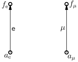
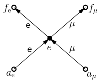
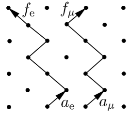
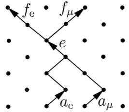
$g\,{A}(a_{\mathrm{e}}\overset{\mathrm{e}}{\to}f_{\mathrm{e}}){A}(e\overset{\mathrm{e}}{\to}e){A}(a_{\mu}\overset{\mu}{\to}e){A}(e\overset{\mu}{\to}f_{\mu})$	$g\,{A}(a_{\mathrm{e}}\overset{\mathrm{e}}{\to}e){A}(e\overset{\mathrm{e}}{\to}f_{\mathrm{e}}){A}(a_{\mu}\overset{\mu}{\to}f_{\mu}){A}(e\overset{\mu}{\to}e)$

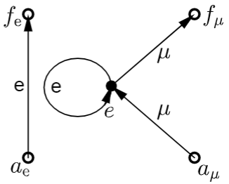
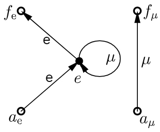
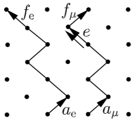
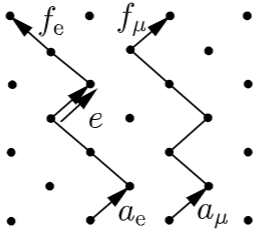
Figure 5: Terms in perturbation expansion, their Feynman diagrams, and collections of loop configurations contributing to the terms (from top to bottom in each cell); see Proposition 21.

The perturbation expansion can be extended to any order in $g$. The terms are depicted as so-called Feynman diagrams as follows (see Figure 5). For each edge in the left side, draw a white vertex. For each edge that is a summation variable in the right side, draw a black vertex. For each factor of the form $A(a\overset{\mathrm{e}}{\to}f)$ or $A(a\overset{\mu}{\to}f)$, draw an arrow from the vertex drawn for $a$ to the vertex drawn for $f$ (a loop, if $a=f$) labeled by letter ‘‘$\mathrm{e}$’’ or ‘‘$\mu$’’ respectively.

We conjecture that those Feynman diagrams have usual properties: each black vertex is the starting point of exactly two arrows labeled by ‘‘$\mathrm{e}$’’ and ‘‘$\mu$’’, is the endpoint of exactly two arrows also labeled by ‘‘$\mathrm{e}$’’ and ‘‘$\mu$’’, and is joined with a white vertex by a sequence of arrows.

Let us give a few comments for specialists. As $\varepsilon\to 0$, the contribution of Feynman diagrams involving loops blows up because $A(e\to e)=1/2$ by Proposition 12 whereas the other arrows are of order $\varepsilon$ by Theorem 2. This suggests that the model has no naive continuum limit. As usual, the true continuum limit requires renormalization, that is, choosing a lattice-dependent coupling $g(\varepsilon)$ in a wise way. Fermi model in $1$ space and $1$ time dimension is known to be renormalizable [29, §III.3, top of p. 180]; thus one expects that the true continuum limit exists. Proving the existence mathematically is as hard as for any other model with interaction.

3.4 Open problems

The new model is only a starting point of the missing Minkowskian lattice quantum field theory. Here we pick up a few informal open problems among a variety of research directions.

We start with the ones relying on Definition 2 only. As a warm-up, we suggest the following.

Problem 1.

(Cf. [19, Theorem 1],[16]) Does expected charge (2) vanish somewhere?

The most shouting problem is to find a large-time asymptotic formula, especially for $|x|>|t|$.

Problem 2.

(Cf. Theorem 3) Prove that for each $m,\varepsilon>0$ and each $(x,t)\in\varepsilon\mathbb{Z}^{2}$ satisfying $1/\sqrt{1+m^{2}\varepsilon^{2}}<|x/t|<1$ we have

$$\tilde{A}_{1}\left(x,t,m,\varepsilon\right) =\frac{i^{\frac{|x|-|t|+\varepsilon}{\varepsilon}}\varepsilon\sqrt{m}\,\theta(x,t,m,\varepsilon)^{1/2}}{\pi((1+m^{2}\varepsilon^{2})x^{2}-t^{2})^{1/4}}K_{1/3}\left(\theta(x,t,m,\varepsilon)\right)\left(1+O_{m,\varepsilon}\left(\frac{1}{|t|}\right)\right),$$

$$\tilde{A}_{2}\left(x,t,m,\varepsilon\right) =\sqrt{\frac{t+x}{t-x}}\frac{i^{\frac{|x|-|t|}{\varepsilon}}\varepsilon\sqrt{m}\,\theta(x,t,m,\varepsilon)^{1/2}}{\pi((1+m^{2}\varepsilon^{2})x^{2}-t^{2})^{1/4}}K_{1/3}\left(\theta(x,t,m,\varepsilon)\right)\left(1+O_{m,\varepsilon}\left(\frac{1}{|t|}\right)\right),$$

where

$$\theta(x,t,m,\varepsilon) :=-\frac{t}{\varepsilon}\,\mathrm{arcosh}\,\frac{m\varepsilon t}{\sqrt{\left(1+m^{2}\varepsilon^{2}\right)\left(t^{2}-x^{2}\right)}}+\frac{x}{\varepsilon}\,\mathrm{arcosh}\,\frac{m\varepsilon x}{\sqrt{t^{2}-x^{2}}}.$$

The limit of small lattice step also deserves attention. Corollary 1 assumes $|x|\neq|t|$, hence misses the main contribution to the charge. Now we ask for the weak limit detecting the peak.

Problem 3.

(Cf. Corollary 1) Find the distributional limits $\lim_{\varepsilon\searrow 0}\widetilde{A}\left(x_{\varepsilon},t_{\varepsilon},{m},{\varepsilon}\right)/{4\varepsilon}$ and $\lim_{\varepsilon\searrow 0}{Q}\left(x_{\varepsilon},t_{\varepsilon},{m},{\varepsilon}\right)/{8\varepsilon^{2}}$ on the whole $\mathbb{R}^{2}$. Is the former limit equal to propagator (4) including the generalized function supported on the lines $t=\pm x$?

The infinite-lattice propagator seems to be unique to satisfy the variety of properties from §§2.4–2.5. But there still could be different finite-lattice propagators with the same limit.

Problem 4.

(Cf. Definition 3, Example 4) Find a combinatorial construction of a finite-lattice propagator having the following properties:

consistency:

it has the same limit (21);

charge conservation:

it satisfies an analogue of Proposition 7 before passing to the limit;

other boundary conditions:

it does not require time-periodic boundary conditions.

The new model describes a free massive spin-$1/2$ quantum field but can be easily adopted to other spins via known relations between propagators for different spins. For instance, spin-$0$ and spin-$1$ massive infinite-lattice propagators are defined to be $\frac{\sqrt{1+m^{2}\varepsilon^{2}}}{2m\varepsilon}\widetilde{A}_{1}\left(x,t,{m},{\varepsilon}\right)$ and $\frac{\sqrt{1+m^{2}\varepsilon^{2}}}{2m\varepsilon}\left(\begin{smallmatrix}\widetilde{A}_{1}\left(x,t,{m},{\varepsilon}\right)&0\\ 0&\widetilde{A}_{1}\left(x,t,{m},{\varepsilon}\right)\end{smallmatrix}\right)$ respectively. Consistency with continuum theory is automatic by Corollary 1 and Proposition 5. However, it is natural to modify the combinatorial definition.

Problem 5.

(Cf. §4.4) Find a combinatorial construction of $\widetilde{A}_{1}\left(x,t,{m},{\varepsilon}\right)$ starting from the Klein–Gordon equation (Proposition 5) instead of the Dirac one, to make the construction symmetric with respect to time reversal $t\mapsto-t$.

Problem 6.

(Cf. Example 1) Find a combinatorial construction of massless spin-$0$, spin-$1/2$, and spin-$1$ infinite-lattice propagators (obtained from the massive ones in the limit $m\to 0$).

Problem 7.

Modify the combinatorial definition of the model with several identical particles (Definition 5) for spin $0$ so that the determinant in Proposition 19 is replaced by the permanent.

The next challenge is to introduce interaction and to prove that the continuum limit of the resulting model has natural physical properties (at least, satisfies Wightman axioms recalled in Appendix B). Particular goals could be quantum electrodynamics and Fermi model (see §3.3).

4 Proofs

Let us present a chart showing the dependence of the above results and further subsections:

Section 4.5 relies only on Theorem 4, Proposition 12, and Lemma 12 among the results proved in §§4.1,4.4. Appendix A contains alternative proofs and is independent from §4.

Throughout this section we use notation (3).

4.1 Fourier integral (Theorem 1, Proposition 1)

In this section we compute the functions in Definition 2 by Fourier method (see Proposition 22). Then we obtain Proposition 1 by contour integration (this step has been already performed in [24]). Finally, we discuss direct consequences (Corollaries 2–6 and Theorem 1). Although the method is analogous to the computation of the continuum propagator, it is the new idea of putting imaginary mass to the dual lattice what makes it successful (see Remark 3).

Proposition 22 (Full space-time Fourier transform).

There exists a unique pair of functions satisfying axioms 1–3 in Definition 2. Under notation $x^{*}:=x+\frac{\varepsilon}{2}$, $t^{*}:=t+\frac{\varepsilon}{2}$, it is given by

$$A_{1}(x,t) =\begin{cases}\frac{\varepsilon^{2}}{4\pi^{2}}\int_{-\pi/\varepsilon}^{\pi/\varepsilon}\int_{-\pi/\varepsilon}^{\pi/\varepsilon}\frac{m\varepsilon-i\delta e^{ip\varepsilon}}{\sqrt{1-\delta^{2}}\sqrt{1+m^{2}\varepsilon^{2}}\cos(\omega\varepsilon)-\cos(p\varepsilon)-im\varepsilon\delta}e^{ipx-i\omega t}\,d\omega dp,&\text{for $2x/\varepsilon$ even},\\ \frac{\varepsilon^{2}}{4\pi^{2}}\int_{-\pi/\varepsilon}^{\pi/\varepsilon}\int_{-\pi/\varepsilon}^{\pi/\varepsilon}\frac{m\varepsilon\sqrt{1-\delta^{2}}e^{i\omega\varepsilon}-i\delta\sqrt{1+m^{2}\varepsilon^{2}}}{\sqrt{1-\delta^{2}}\sqrt{1+m^{2}\varepsilon^{2}}\cos(\omega\varepsilon)-\cos(p\varepsilon)-im\varepsilon\delta}e^{ipx^{*}-i\omega t^{*}}\,d\omega dp,&\text{for $2x/\varepsilon$ odd};\end{cases}$$

$$A_{2}(x,t) =\begin{cases}\frac{\varepsilon^{2}}{4\pi^{2}}\int_{-\pi/\varepsilon}^{\pi/\varepsilon}\int_{-\pi/\varepsilon}^{\pi/\varepsilon}\frac{\sqrt{1-\delta^{2}}\sqrt{1+m^{2}\varepsilon^{2}}e^{-i\omega\varepsilon}-e^{ip\varepsilon}-im\varepsilon\delta}{\sqrt{1-\delta^{2}}\sqrt{1+m^{2}\varepsilon^{2}}\cos(\omega\varepsilon)-\cos(p\varepsilon)-im\varepsilon\delta}e^{ipx-i\omega t}\,d\omega dp,&\text{for $2x/\varepsilon$ even},\\ \frac{\varepsilon^{2}}{4\pi^{2}}\int_{-\pi/\varepsilon}^{\pi/\varepsilon}\int_{-\pi/\varepsilon}^{\pi/\varepsilon}\frac{\sqrt{1+m^{2}\varepsilon^{2}}e^{-ip\varepsilon}-\sqrt{1-\delta^{2}}e^{i\omega\varepsilon}}{\sqrt{1-\delta^{2}}\sqrt{1+m^{2}\varepsilon^{2}}\cos(\omega\varepsilon)-\cos(p\varepsilon)-im\varepsilon\delta}e^{ipx^{*}-i\omega t^{*}}\,d\omega dp,&\text{for $2x/\varepsilon$ odd}.\end{cases}$$

Proof.

Substituting axiom 2 into axiom 1 for each $(x,t)\in\varepsilon\mathbb{Z}^{2}$, we get

$$A_{1}(x,t) =\frac{A_{1}(x+\varepsilon,t-\varepsilon)+im\varepsilon\delta A_{1}(x,t-\varepsilon)-i\delta A_{2}(x+\varepsilon,t-\varepsilon)+m\varepsilon A_{2}(x,t-\varepsilon)}{\sqrt{1+m^{2}\varepsilon^{2}}\sqrt{1-\delta^{2}}},$$ (23)

$$A_{2}(x,t) =\frac{i\delta A_{1}(x-\varepsilon,t-\varepsilon)-m\varepsilon A_{1}(x,t-\varepsilon)+A_{2}(x-\varepsilon,t-\varepsilon)+im\varepsilon\delta A_{2}(x,t-\varepsilon)}{\sqrt{1+m^{2}\varepsilon^{2}}\sqrt{1-\delta^{2}}}+2\delta_{x0}\delta_{t0}.$$

It suffices to solve system (23) on $\varepsilon\mathbb{Z}^{2}$ (that is, for $2x/\varepsilon$ even) under the restriction given by axiom 3; then the values for $2x/\varepsilon$ odd are uniquely determined (and computed) by axiom 2.

We use Fourier method. To a function $A_{k}(x,t)$ satisfying axiom 3 assign the Fourier series

$$\widehat{A}_{k}(p,\omega):\overset{L^{2}}{=}\sum_{(x,t)\in\varepsilon\mathbb{Z}^{2}}A_{k}(x,t)e^{-ipx+i\omega t}\in L^{2}([-\pi/\varepsilon,\pi/\varepsilon]^{2}).$$

Here the summands are understood as functions on $[-\pi/\varepsilon,\pi/\varepsilon]^{2}$ and mean-square convergence of the series is assumed. By Plancherel theorem, this assignment is a bijection between the space of functions satisfying axiom 3 and the space $L^{2}([-\pi/\varepsilon,\pi/\varepsilon]^{2})$ of square-integrable functions $[-\pi/\varepsilon,\pi/\varepsilon]^{2}\to\mathbb{C}$ up to change on a set of measure zero.

Under this bijection, the shifts $x\mapsto x\pm\varepsilon$ and $t\mapsto t-\varepsilon$ are taken to multiplication by $e^{\pm ip\varepsilon}$ and $e^{i\omega\varepsilon}$ respectively, and $\delta_{x0}\delta_{t0}$ is taken to $1$. Thus (23) is transformed to the following equality almost everywhere

$$\begin{pmatrix}\widehat{A}_{1}(p,\omega)\\ \widehat{A}_{2}(p,\omega)\end{pmatrix}=\frac{e^{i\omega\varepsilon}}{\sqrt{1+m^{2}\varepsilon^{2}}\sqrt{1-\delta^{2}}}\begin{pmatrix}e^{ip\varepsilon}+im\varepsilon\delta&-i\delta e^{ip\varepsilon}+m\varepsilon\\ i\delta e^{-ip\varepsilon}-m\varepsilon&e^{-ip\varepsilon}+im\varepsilon\delta\end{pmatrix}\begin{pmatrix}\widehat{A}_{1}(p,\omega)\\ \widehat{A}_{2}(p,\omega)\end{pmatrix}+\begin{pmatrix}0\\ 2\end{pmatrix}.$$ (24)

The resulting $2\times 2$ linear system has the unique solution (this is checked in [25, §1])

$$\widehat{A}_{1}(p,\omega) =\frac{m\varepsilon-i\delta e^{ip\varepsilon}}{\sqrt{1-\delta^{2}}\sqrt{1+m^{2}\varepsilon^{2}}\cos(\omega\varepsilon)-\cos(p\varepsilon)-im\varepsilon\delta},$$

$$\widehat{A}_{2}(p,\omega) =\frac{\sqrt{1-\delta^{2}}\sqrt{1+m^{2}\varepsilon^{2}}e^{-i\omega\varepsilon}-e^{ip\varepsilon}-im\varepsilon\delta}{\sqrt{1-\delta^{2}}\sqrt{1+m^{2}\varepsilon^{2}}\cos(\omega\varepsilon)-\cos(p\varepsilon)-im\varepsilon\delta}.$$

It belongs to $L^{2}([-\pi/\varepsilon,\pi/\varepsilon]^{2})$ because $m,\varepsilon,\delta>0$ and the denominator vanishes nowhere. Now the formula for the Fourier coefficients gives the desired expressions in the proposition. ∎

Remark 3.

This argument shows that for $\delta=0$ axioms 1–3 are inconsistent even if $m$ has imaginary part because $\widehat{A}_{k}(p,\omega)$ blows up at $(\pi/2\varepsilon,\pi/2\varepsilon)$. Thus Step 2 in §2.1 is necessary.

Passing to the limit $\delta\searrow 0$ in Proposition 22 and using $\frac{\varepsilon}{2\pi}\int_{-\pi/\varepsilon}^{\pi/\varepsilon}e^{ipx}\,dp=\delta_{x0}$ for $x\in\varepsilon\mathbb{Z}$, we get the following result.

Proposition 23 (Full space-time Fourier transform).

For each $(x,t)\in\varepsilon\mathbb{Z}^{2}$ we have

$$\tilde{A}_{1}(x,t) =\lim_{\delta\searrow 0}\frac{m\varepsilon^{3}}{4\pi^{2}}\int_{-\pi/\varepsilon}^{\pi/\varepsilon}\int_{-\pi/\varepsilon}^{\pi/\varepsilon}\frac{e^{ipx-i\omega t}\,d\omega dp}{\sqrt{1+m^{2}\varepsilon^{2}}\cos(\omega\varepsilon)-\cos(p\varepsilon)-i\delta},$$

$$\tilde{A}_{2}(x,t) =\lim_{\delta\searrow 0}\frac{-i\varepsilon^{2}}{4\pi^{2}}\int_{-\pi/\varepsilon}^{\pi/\varepsilon}\int_{-\pi/\varepsilon}^{\pi/\varepsilon}\frac{\sqrt{1+m^{2}\varepsilon^{2}}\sin(\omega\varepsilon)+\sin(p\varepsilon)}{\sqrt{1+m^{2}\varepsilon^{2}}\cos(\omega\varepsilon)-\cos(p\varepsilon)-i\delta}e^{ipx-i\omega t}\,d\omega dp+\delta_{x0}\delta_{t0}.$$

Proof of Proposition 1.

This follows from Proposition 23 and [24, Proposition 17], which states that the right-hand sides of Proposition 23 and Proposition 1 are equal (and in particular, the limits in Proposition 23 exist). ∎

Performing changes of variables $(p,\omega)\mapsto(p\varepsilon,\omega\varepsilon)$, $(\pi/\varepsilon-p,\pi/\varepsilon-\omega)$, $(\pm p,-\omega)$ in the integrals from Proposition 23, one gets the following three immediate corollaries.

Corollary 2 (Scaling symmetry).

For each $k\in\{1,2\}$ and $(x,t)\in\varepsilon\mathbb{Z}^{2}$ we have $\widetilde{A}_{k}(x,t,m,\varepsilon)=\widetilde{A}_{k}(x/\varepsilon,t/\varepsilon,m\varepsilon,1)$.

Corollary 3 (Alternation of real and imaginary values).

Let $k\in\{1,2\}$ and $(x,t)\in\varepsilon\mathbb{Z}^{2}$. If $(x+t)/\varepsilon+k$ is even (respectively, odd), then $\widetilde{A}_{k}(x,t)$ is real (respectively, purely imaginary).

Corollary 4 (Skew symmetry).

For each $(x,t)\in\varepsilon\mathbb{Z}^{2}$, where $(x,t)\neq(0,0)$, we have $\widetilde{A}_{1}(x,t)=\widetilde{A}_{1}(x,-t)=\widetilde{A}_{1}(-x,-t)$ and $\widetilde{A}_{2}(x,t)=-\widetilde{A}_{2}(-x,-t)$.

Proof of Theorem 1.

The existence and uniqueness of $A_{k}(x,t,m,\varepsilon,\delta)$ is Proposition 22. The existence of limit (21) and the required equalities follow from Proposition 1, Corollary 4, and [24, Proposition 12], which states that the integrals from Proposition 1 equal $a_{1}(x,t+\varepsilon,m,\varepsilon)$ and $a_{2}(x+\varepsilon,t+\varepsilon,m,\varepsilon)$ for $t\geq 0$ and appropriate parity of $(x+t)/\varepsilon$. The rest is Corollary 3. ∎

Corollary 5 (Symmetry).

For each $(x,t)\in\varepsilon\mathbb{Z}^{2}$ we have $(t-x)\widetilde{A}_{2}(x,t)=(t+x)\widetilde{A}_{2}(-x,t)$.

Proof.

Assume that $x\neq 0$. Changing the sign of the variable $p$ in Proposition 23 we get

$$\widetilde{A}_{2}(-x,t)=\lim_{\delta\searrow 0}\frac{-i\varepsilon^{2}}{4\pi^{2}}\int_{-\pi/\varepsilon}^{\pi/\varepsilon}\int_{-\pi/\varepsilon}^{\pi/\varepsilon}\frac{\sqrt{1+m^{2}\varepsilon^{2}}\sin(\omega\varepsilon)-\sin(p\varepsilon)}{\sqrt{1+m^{2}\varepsilon^{2}}\cos(\omega\varepsilon)-\cos(p\varepsilon)-i\delta}e^{ipx-i\omega t}\,d\omega dp.$$

Adding the expression for $\widetilde{A}_{2}(x,t)$ from Proposition 23 and integrating by parts twice we get

$$\widetilde{A}_{2}(x,t)+\widetilde{A}_{2}(-x,t)=\lim_{\delta\searrow 0}\frac{-i\varepsilon^{2}}{2\pi^{2}}\int_{-\pi/\varepsilon}^{\pi/\varepsilon}\int_{-\pi/\varepsilon}^{\pi/\varepsilon}\frac{\sqrt{1+m^{2}\varepsilon^{2}}\sin(\omega\varepsilon)}{\sqrt{1+m^{2}\varepsilon^{2}}\cos(\omega\varepsilon)-\cos(p\varepsilon)-i\delta}e^{ipx-i\omega t}\,d\omega dp=\\ =\lim_{\delta\searrow 0}\frac{i\varepsilon^{2}}{2\pi^{2}}\int_{-\pi/\varepsilon}^{\pi/\varepsilon}\int_{-\pi/\varepsilon}^{\pi/\varepsilon}\frac{\sqrt{1+m^{2}\varepsilon^{2}}\sin(\omega\varepsilon)\sin(p\varepsilon)\varepsilon}{(\sqrt{1+m^{2}\varepsilon^{2}}\cos(\omega\varepsilon)-\cos(p\varepsilon)-i\delta)^{2}}\cdot\frac{e^{ipx-i\omega t}}{ix}\,d\omega dp=\\ =\lim_{\delta\searrow 0}\frac{-i\varepsilon^{2}}{2\pi^{2}}\int_{-\pi/\varepsilon}^{\pi/\varepsilon}\int_{-\pi/\varepsilon}^{\pi/\varepsilon}\frac{\sin(p\varepsilon)(it)e^{ipx-i\omega t}\,d\omega dp}{(\sqrt{1+m^{2}\varepsilon^{2}}\cos(\omega\varepsilon)-\cos(p\varepsilon)-i\delta)(ix)}=\frac{t}{x}\left(\widetilde{A}_{2}(x,t)-\widetilde{A}_{2}(-x,t)\right).$$

Here in the second equality, we integrate the exponential and differentiate the remaining factor with respect to $p$. In the third equality, we differentiate the exponential and integrate the remaining factor with respect to $\omega$. The resulting identity is equivalent to the required one. ∎

For the proof of Theorem 2, we halve the integration interval $[-\pi/\varepsilon,\pi/\varepsilon]$ in Proposition 1.

Corollary 6.

For each $(x,t)\in\varepsilon\mathbb{Z}^{2}$, where $t\geq 0$, we have

$$\widetilde{A}_{1}(x,t) =\begin{cases}\mathrm{Re}\,\left(\frac{im\varepsilon^{2}}{\pi}\int_{-\pi/2\varepsilon}^{\pi/2\varepsilon}\frac{e^{ipx-i\omega_{p}t}\,dp}{\sqrt{m^{2}\varepsilon^{2}+\sin^{2}(p\varepsilon)}}\right),&\text{for }(x+t)/\varepsilon\text{ odd};\\ \mathrlap{i\mathrm{Im}\,\left(\frac{im\varepsilon^{2}}{\pi}\int_{-\pi/2\varepsilon}^{\pi/2\varepsilon}\frac{e^{ipx-i\omega_{p}t}\,dp}{\sqrt{m^{2}\varepsilon^{2}+\sin^{2}(p\varepsilon)}}\right),}\hphantom{i\mathrm{Im}\,\left(\frac{\varepsilon}{\pi}\int_{-\pi/2\varepsilon}^{\pi/2\varepsilon}\left(1+\frac{\sin(p\varepsilon)}{\sqrt{m^{2}\varepsilon^{2}+\sin^{2}(p\varepsilon)}}\right)e^{ipx-i\omega_{p}t}\,dp\right),}&\text{for }(x+t)/\varepsilon\text{ even};\end{cases}$$

$$\widetilde{A}_{2}(x,t) =\begin{cases}\mathrm{Re}\,\left(\frac{\varepsilon}{\pi}\int_{-\pi/2\varepsilon}^{\pi/2\varepsilon}\left(1+\frac{\sin(p\varepsilon)}{\sqrt{m^{2}\varepsilon^{2}+\sin^{2}(p\varepsilon)}}\right)e^{ipx-i\omega_{p}t}\,dp\right),&\text{for }(x+t)/\varepsilon\text{ even};\\ i\mathrm{Im}\,\left(\frac{\varepsilon}{\pi}\int_{-\pi/2\varepsilon}^{\pi/2\varepsilon}\left(1+\frac{\sin(p\varepsilon)}{\sqrt{m^{2}\varepsilon^{2}+\sin^{2}(p\varepsilon)}}\right)e^{ipx-i\omega_{p}t}\,dp\right),&\text{for }(x+t)/\varepsilon\text{ odd}.\end{cases}$$

Proof.

This follows from Proposition 1 by the change of variable $p\mapsto\pi/\varepsilon-p$. For instance,

$$\widetilde{A}_{1}(x,t)=\frac{im\varepsilon^{2}}{2\pi}\int_{-\pi/2\varepsilon}^{\pi/2\varepsilon}\frac{e^{ipx-i\omega_{p}t}\,dp}{\sqrt{m^{2}\varepsilon^{2}+\sin^{2}(p\varepsilon)}}+\frac{im\varepsilon^{2}}{2\pi}\int_{\pi/2\varepsilon}^{3\pi/2\varepsilon}\frac{e^{ipx-i\omega_{p}t}\,dp}{\sqrt{m^{2}\varepsilon^{2}+\sin^{2}(p\varepsilon)}}=\\ =\frac{im\varepsilon^{2}}{2\pi}\int_{-\pi/2\varepsilon}^{\pi/2\varepsilon}\frac{e^{ipx-i\omega_{p}t}\,dp}{\sqrt{m^{2}\varepsilon^{2}+\sin^{2}(p\varepsilon)}}+(-1)^{(x+t)/\varepsilon}\frac{im\varepsilon^{2}}{2\pi}\int_{-\pi/2\varepsilon}^{\pi/2\varepsilon}\frac{e^{-ipx+i\omega_{p}t}\,dp}{\sqrt{m^{2}\varepsilon^{2}+\sin^{2}(p\varepsilon)}},\quad\text{as required.}\\[-36.98866pt]$$

∎

4.2 Asymptotic formulae (Theorem 2, Corollary 1)

In this subsection we prove Theorem 2 and Corollary 1.

First let us outline the plan of the argument. We perform the Fourier transform and estimate the difference of the resulting oscillatory integrals for the discrete and continuum models, using tails exchange and non-stationary-phase method. The proof of (9) consists of $3$ steps:

Step 1:

we replace the integration interval in the Fourier integral for the continuum model by the one from the discrete model (cutting off large momenta);

Step 2:

we replace the phase in the discrete model by the one from the continuum model;

Step 3:

we estimate the difference of the resulting integrals for the continuum and discrete models for small and intermediate momenta.

In the proof of (10), we first subtract the massless propagator from the massive one to make the Fourier integral convergent. The integral for the continuum model is as follows.

Lemma 1.

Under notation (11), for each $m>0$, $t\geq 0$, and $x\neq\pm t$ we have

$$G^{F}_{11}(x,t,m) =\frac{im}{4\pi}\int_{-\infty}^{+\infty}\frac{e^{ipx-i\sqrt{m^{2}+p^{2}}t}\,dp}{\sqrt{m^{2}+p^{2}}},$$

where the integral is understood as a conditionally convergent improper Riemann integral.

Proof.

For $t>|x|$, use the change of variables $q=tp-x\sqrt{m^{2}+p^{2}}$ and [10, 8.421.11, 8.405.1]:

$$\frac{im}{4\pi}\int_{-\infty}^{+\infty}\frac{e^{ipx-i\sqrt{m^{2}+p^{2}}t}\,dp}{\sqrt{m^{2}+p^{2}}}=\frac{im}{4\pi}\int_{-\infty}^{+\infty}\frac{e^{-i\sqrt{m^{2}(t^{2}-x^{2})+q^{2}}}\,dq}{\sqrt{m^{2}(t^{2}-x^{2})+q^{2}}}=G^{F}_{11}(x,t,m).$$

For $0\leq t<|x|$, use the change of variables $q=xp-t\sqrt{m^{2}+p^{2}}$ and [10, 8.432.5]. ∎

Proof of formula (9) in Theorem 2.

In the case when $|x|>|t|$ and $(x+t)/\varepsilon$ is odd, formula (9) follows from Theorem 1 and Definition 1; thus we exclude this case in what follows. We may assume that $x,t\geq 0$ because  (9) is invariant under the transformations $(x,t)\mapsto(\pm x,\pm t)$ by Corollaries 4–5. Assume that $(x+t)/\varepsilon$ is even; otherwise the proof is the same up to an obvious modification of the very first inequality below. Use notation (11). Formula (9) will follow from

$$\left|\widetilde{A}_{1}(x,t,m,\varepsilon)-4\varepsilon\,\mathrm{Im}G^{F}_{11}(x,t,m)\right|\leq\left|\frac{im\varepsilon^{2}}{\pi}\int\limits_{-\pi/2\varepsilon}^{\pi/2\varepsilon}\frac{e^{ipx-i\omega_{p}t}\,dp}{\sqrt{m^{2}\varepsilon^{2}+\sin^{2}(p\varepsilon)}}-\frac{im\varepsilon}{\pi}\int\limits_{-\infty}^{+\infty}\frac{e^{ipx-i\sqrt{m^{2}+p^{2}}t}\,dp}{\sqrt{m^{2}+p^{2}}}\right|\\ \leq\frac{m\varepsilon}{\pi}\left|\int_{|p|\geq\pi/2\varepsilon}\frac{e^{ipx-i\sqrt{m^{2}+p^{2}}t}\,dp}{\sqrt{m^{2}+p^{2}}}\right|+\frac{m\varepsilon}{\pi}\left|\int_{|p|\leq\pi/2\varepsilon}\frac{\varepsilon\left(e^{ipx-i\omega_{p}t}-e^{ipx-i\sqrt{m^{2}+p^{2}}t}\right)\,dp}{\sqrt{m^{2}\varepsilon^{2}+\sin^{2}(p\varepsilon)}}\right|\\ +\frac{m\varepsilon}{\pi}\left|\int_{|p|\leq\pi/2\varepsilon}\left(\frac{\varepsilon}{\sqrt{m^{2}\varepsilon^{2}+\sin^{2}(p\varepsilon)}}-\frac{1}{\sqrt{m^{2}+p^{2}}}\right)e^{ipx-i\sqrt{m^{2}+p^{2}}t}\,dp\right|=\\ =m\varepsilon\,O\left(\frac{\varepsilon}{|x-t|}+\frac{m\varepsilon(x+t)}{s}\right)+m\varepsilon\,O\left(m^{2}t\varepsilon\right)+m\varepsilon\,O\left(\frac{\varepsilon}{|x-t|}+\frac{m\varepsilon(x+t)}{s}\right)=m\varepsilon\,O\left(\varepsilon\Delta\right).$$

Here the first inequality follows from Corollary 6, Lemma 1, and the inequality $|\mathrm{Im}\,z-\mathrm{Im}\,w|\leq|z-w|$. The second inequality is straightforward. The obtained $3$ integrals are estimated below in Steps 1–3 respectively. The last bound follows from $2m(x+t)/s\leq\Delta$. Below we restrict the integrals to $p\geq 0$; the argument for $p<0$ is analogous. The estimates are slightly different for $\varepsilon<s/m(x+t)$ and $\varepsilon>s/m(x+t)$. Denote

$$\varepsilon_{+} :=\max\{\varepsilon,s/m(x+t)\};$$ (25)

$$\varepsilon_{-} :=\min\{\varepsilon,s/m(x+t)\}.$$

We use the following known result.

Lemma 2 (First derivative test).

[11, Lemma 5.1.2] Let $\alpha,\beta\in\mathbb{R}$ and $\alpha<\beta$. Assume that $f\in C^{1}[\alpha,\beta]$ has monotone nonvanishing derivative; then for each $g\in C^{0}[\alpha,\beta]$ we have

$$\left|\int_{\alpha}^{\beta}g(p)e^{if(p)}\,dp\right|\leq\frac{2\max_{[\alpha,\beta]}|g|+2V_{\alpha}^{\beta}(g)}{\min_{[\alpha,\beta]}|f^{\prime}|}.$$ (26)

Step 1. Apply Lemma 2 for $\alpha=\pi/2\varepsilon_{-}$, $\beta\to+\infty$, $f(p):=px-\sqrt{m^{2}+p^{2}}\,t$, and $g(p):=1/\sqrt{m^{2}+p^{2}}$. The derivative $f^{\prime}(p)$ is monotone because $f^{\prime\prime}(p)=-m^{2}t/(m^{2}+p^{2})^{3/2}\leq 0$. Since $g(p)\searrow 0$ as $p\to+\infty$, it follows that the numerator in the right side of (26) tends to $4g(\pi/2\varepsilon_{-})\leq 8\varepsilon_{-}/\pi=O(\varepsilon)$ as $\beta\to+\infty$. To bound the denominator from below (and in particular to check the assumption $f^{\prime}(p)\neq 0$), we need a lemma.

Lemma 3.

If $p\geq\pi m(x+t)/2s$ then $|x-tp/\sqrt{m^{2}+p^{2}}|\geq|x-t|/4$.

Proof.

We may assume that $x\neq 0$. Since $p\geq\pi m(x+t)/2s\geq\pi mx/2\sqrt{|t^{2}-x^{2}|}$ it follows that $m/p\leq 1$ and ${m^{2}}/{p^{2}}=\eta{(t^{2}-x^{2})}/{x^{2}}$ for some $\eta\in[-4/\pi^{2};4/\pi^{2}]\subset[-1/2;1/2]$. Thus

$$\left|x-t\frac{p}{\sqrt{m^{2}+p^{2}}}\right|=\frac{\left|x^{2}\left(1+m^{2}/p^{2}\right)-t^{2}\right|}{x\left(1+m^{2}/p^{2}\right)+t\sqrt{1+m^{2}/p^{2}}}=\frac{(1-\eta)|t^{2}-x^{2}|}{x\left(1+m^{2}/p^{2}\right)+t\sqrt{1+m^{2}/p^{2}}}\geq\frac{|x-t|}{4}.\vspace{-0.6cm}$$

∎

Since $\alpha=\pi/2\varepsilon_{-}\geq\pi m(x+t)/2s$, by Lemmas 2–3 we get $\int_{\pi/2\varepsilon_{-}}^{+\infty}\frac{e^{ipx-i\sqrt{m^{2}+p^{2}}t}\,dp}{\sqrt{m^{2}+p^{2}}}=O\left(\frac{\varepsilon}{|x-t|}\right)$.

For $\varepsilon\leq s/m(x+t)$, which is equivalent to $\varepsilon_{-}=\varepsilon$, this completes step 1.

For $\varepsilon>s/m(x+t)$ we need an additional bound

$$\left|\int_{\pi/2\varepsilon}^{\pi/2\varepsilon_{-}}\frac{e^{ipx-i\sqrt{m^{2}+p^{2}}t}\,dp}{\sqrt{m^{2}+p^{2}}}\right|\leq\int_{\pi/2\varepsilon}^{\pi/2\varepsilon_{-}}\frac{dp}{\pi/2\varepsilon}\leq\frac{\pi/2\varepsilon_{-}}{\pi/2\varepsilon}=\frac{m\varepsilon(x+t)}{s}.$$

Step 2. Using that $1-e^{iz}=O(|z|)$ for $z\in\mathbb{R}$ and $\sin z>z/2$ for $0<z<\pi/2$ we get

$$\int_{0}^{\pi/2\varepsilon}\frac{\varepsilon\left(e^{ipx-i\omega_{p}t}-e^{ipx-i\sqrt{m^{2}+p^{2}}t}\right)\,dp}{\sqrt{m^{2}\varepsilon^{2}+\sin^{2}(p\varepsilon)}}=\int_{0}^{\pi/2\varepsilon}\frac{\left(1-e^{i\omega_{p}t-i\sqrt{m^{2}+p^{2}}t}\right)\varepsilon e^{ipx-i\omega_{p}t}\,dp}{\sqrt{m^{2}\varepsilon^{2}+\sin^{2}(p\varepsilon)}}=\\ =O\left(\int_{0}^{\pi/2\varepsilon}\frac{\left|\omega_{p}-\sqrt{m^{2}+p^{2}}\right|\varepsilon t\,dp}{\sqrt{m^{2}\varepsilon^{2}+\sin^{2}(p\varepsilon)}}\right)=O\left(\int_{0}^{\pi/2\varepsilon}\frac{m^{2}\varepsilon^{2}t\sqrt{m^{2}+p^{2}}\,dp}{\sqrt{m^{2}+p^{2}}}\right)=O\left(\frac{\pi}{2\varepsilon}\cdot m^{2}\varepsilon^{2}t\right)=O(m^{2}t\varepsilon).$$

Here the third estimate is proved in the following lemma.

Lemma 4.

For $|p|\leq\pi/2\varepsilon$ we have

$$\omega_{p}=\sqrt{p^{2}+m^{2}}+O\left(m^{2}\varepsilon^{2}\sqrt{p^{2}+m^{2}}\right)\qquad\text{ and }\qquad\frac{\partial\omega_{p}}{\partial p}=\frac{\sin p\varepsilon}{\sqrt{\sin^{2}p\varepsilon+m^{2}\varepsilon^{2}}}=\frac{p}{\sqrt{p^{2}+m^{2}}}+O(m^{2}\varepsilon^{2}).$$

Proof.

First we estimate the derivative. By the Lagrange theorem, there is $\varepsilon^{\prime}\in[0,\varepsilon]$ such that

$$\frac{\sin p\varepsilon}{\sqrt{\sin^{2}p\varepsilon+m^{2}\varepsilon^{2}}}-\frac{p}{\sqrt{p^{2}+m^{2}}}=\left.\frac{\partial}{\partial\varepsilon}\left(\frac{\sin p\varepsilon}{\sqrt{\sin^{2}p\varepsilon+m^{2}\varepsilon^{2}}}\right)\right|_{\varepsilon=\varepsilon^{\prime}}\cdot\varepsilon=\\ =\left.\frac{m^{2}\varepsilon(p\varepsilon\cos p\varepsilon-\sin p\varepsilon)}{(\sin^{2}p\varepsilon+m^{2}\varepsilon^{2})^{3/2}}\right|_{\varepsilon=\varepsilon^{\prime}}\cdot\varepsilon=O(m^{2}\varepsilon^{2})$$

because $\sin z-z\cos z=O(z^{3})$ and $\sin z>z/2$ for $0<z<\pi/2$.

Now we estimate $\omega_{p}$. By the Lagrange theorem, there is $m^{\prime}\in[0,m]$ such that

$$\omega_{0}=\left.\frac{\partial\omega_{0}}{\partial m}\right|_{m=m^{\prime}}\cdot m=\left.\frac{1}{1+m^{2}\varepsilon^{2}}\right|_{m=m^{\prime}}\cdot m=m+O(m^{3}\varepsilon^{2}).$$

Then by the estimate for the derivative $\frac{\partial\omega_{p}}{\partial p}$, for some $p^{\prime}\in[0,p]$ we have

$$\omega_{p}-\sqrt{p^{2}+m^{2}}=\omega_{0}-m+\left.\left(\frac{\partial\omega_{p}}{\partial p}-\frac{p}{\sqrt{p^{2}+m^{2}}}\right)\right|_{p=p^{\prime}}\cdot p=O(m^{2}\varepsilon^{2}\sqrt{p^{2}+m^{2}}).\vspace{-1.1cm}$$

∎

Step 3. We have

$$\int\limits_{0}^{2\pi/\varepsilon_{+}}\left(\frac{\varepsilon}{\sqrt{m^{2}\varepsilon^{2}+\sin^{2}(p\varepsilon)}}-\frac{1}{\sqrt{m^{2}+p^{2}}}\right)e^{ipx-i\sqrt{m^{2}+p^{2}}t}\,dp=O\left(\int\limits_{0}^{2\pi/\varepsilon_{+}}p\varepsilon^{2}\,dp\right)=O\left(\frac{\varepsilon^{2}}{\varepsilon_{+}^{2}}\right)=O\left(\frac{\varepsilon m(x+t)}{s}\right).$$

Here the first estimate is proved in the following lemma.

Lemma 5.

For $0\leq p\leq\pi/2\varepsilon$ we have $\frac{\varepsilon}{\sqrt{\sin^{2}p\varepsilon+m^{2}\varepsilon^{2}}}-\frac{1}{\sqrt{p^{2}+m^{2}}}=O(p\varepsilon^{2}).$

Proof.

By the Lagrange theorem, for some $\varepsilon^{\prime}\in(0;\varepsilon)$ we have

$$\frac{\varepsilon}{\sqrt{\sin^{2}p\varepsilon+m^{2}\varepsilon^{2}}}-\frac{1}{\sqrt{p^{2}+m^{2}}}=\left.\frac{\partial}{\partial\varepsilon}\frac{\varepsilon}{\sqrt{\sin^{2}p\varepsilon+m^{2}\varepsilon^{2}}}\right|_{\varepsilon=\varepsilon^{\prime}}\cdot\varepsilon=\left.\frac{\sin p\varepsilon(\sin p\varepsilon-p\varepsilon\cos p\varepsilon)}{(\sin^{2}p\varepsilon+m^{2}\varepsilon^{2})^{3/2}}\right|_{\varepsilon=\varepsilon^{\prime}}\cdot\varepsilon=O(p\varepsilon^{2})$$

because $\sin z-z\cos z=O(z^{3})$ and $z/2<\sin z<z$ for $0<z<\pi/2$. ∎

For $\varepsilon<s/m(x+t)$ we need an additional bound:

$$\int_{\pi/2\varepsilon_{+}}^{\pi/2\varepsilon}\left(\frac{\varepsilon}{\sqrt{m^{2}\varepsilon^{2}+\sin^{2}(p\varepsilon)}}-\frac{1}{\sqrt{m^{2}+p^{2}}}\right)e^{ipx-i\sqrt{m^{2}+p^{2}}t}\,dp=O\left(\frac{\varepsilon}{|x-t|}\right)$$

obtained by applying Lemma 2 for $g(p):={\varepsilon}/{\sqrt{m^{2}\varepsilon^{2}+\sin^{2}(p\varepsilon)}}-1/\sqrt{m^{2}+p^{2}}$ and $f(p)=px-\sqrt{m^{2}+p^{2}}\,t$. The lower bound for the denominator of (26) is obtained by Lemma 3. The numerator is at most $4g(\pi/2\varepsilon)=O(\varepsilon+2\varepsilon/\pi)=O(\varepsilon)$ by the following lemma. ∎

Lemma 6.

The function $g(p):={\varepsilon}/{\sqrt{m^{2}\varepsilon^{2}+\sin^{2}(p\varepsilon)}}-1/\sqrt{m^{2}+p^{2}}$ increases on $[0,\pi/2\varepsilon]$.

Proof.

It suffices to prove that

$$\frac{\partial g}{\partial p}=-\frac{\varepsilon^{2}\sin(p\varepsilon)\cos(p\varepsilon)}{(m^{2}\varepsilon^{2}+\sin^{2}(p\varepsilon))^{3/2}}+\frac{p}{(m^{2}+p^{2})^{3/2}}\geq 0.$$

Since this expression clearly tends to $0$ as $\varepsilon\to 0$, it suffices to prove that

$$\frac{\partial^{2}g}{\partial p\partial\varepsilon}=\frac{\varepsilon\left(2\sin^{2}p\varepsilon\left(p\varepsilon(1-\cos p\varepsilon)^{2}+2(p\varepsilon-\sin p\varepsilon)\cos p\varepsilon\right)+m^{2}\varepsilon^{2}(\sin 2p\varepsilon-2p\varepsilon\cos 2p\varepsilon)\right)}{2(m^{2}\varepsilon^{2}+\sin^{2}(p\varepsilon))^{5/2}}\geq 0.$$

The equality and the inequality follow from [25, §3] and $\sin z\leq z\leq\tan z$ for $z\in[0,\pi/2]$. ∎

This completes the proof of (9). For the proof of (10) we need two lemmas establishing the Fourier integral for the continuum model.

Lemma 7.

Under notation (11) and (6), for each $m,t\geq 0$ and $x\neq\pm t$ we have

$$G^{F}_{12}(x,t,m)-G^{F}_{12}(x,t,0) =\frac{1}{4\pi}\int_{-\infty}^{+\infty}\left(\left(1+\frac{p}{\sqrt{m^{2}+p^{2}}}\right)e^{-i\sqrt{m^{2}+p^{2}}t}-\left(1+\mathrm{sgn}(p)\right)e^{-i|p|t}\right)e^{ipx}\,dp.$$

where the integral is understood as conditionally convergent improper Riemann integral.

Proof.

This is the limiting case $n\searrow 0$ of the following formula:

$$G^{F}_{12}(x,t,m)-G^{F}_{12}(x,t,n)=\left(\frac{\partial}{\partial t}-\frac{\partial}{\partial x}\right)\left(\frac{G^{F}_{11}(x,t,m)}{m}-\frac{G^{F}_{11}(x,t,n)}{n}\right)=\\ =\int_{-\infty}^{+\infty}\left(\frac{\partial}{\partial t}-\frac{\partial}{\partial x}\right)\left(\frac{e^{ipx-i\sqrt{m^{2}+p^{2}}t}}{\sqrt{m^{2}+p^{2}}}-\frac{e^{ipx-i\sqrt{n^{2}+p^{2}}t}}{\sqrt{n^{2}+p^{2}}}\right)\frac{i\,dp}{4\pi}=\int_{-\infty}^{+\infty}\left(e^{ipx-i\sqrt{m^{2}+p^{2}}t}-e^{ipx-i\sqrt{n^{2}+p^{2}}t}\right)\,\frac{dp}{4\pi}+\\ +\int_{-\infty}^{+\infty}\left(\frac{p}{\sqrt{m^{2}+p^{2}}}e^{-i\sqrt{m^{2}+p^{2}}t}-\frac{p}{\sqrt{n^{2}+p^{2}}}e^{-i\sqrt{n^{2}+p^{2}}t}\right)\frac{e^{ipx}\,dp}{4\pi}$$

Here we first applied [10, 8.473.4,5], then Lemma 1. We can change the order of the differentiation and the integration (and pass to the limit $n\searrow 0$ under the integral) by [30, Proposition 6 in §2.3 in Ch. 7] because the latter two integrals converge uniformly on compact subsets of $\mathbb{R}^{2}\setminus\{|x|=|t|\}$ by the following lemma. ∎

Lemma 8.

For each $m,n,x,t\geq 0$, $\alpha>0$, and $x\neq t$ we have

$$\int_{\alpha}^{+\infty}\left(\frac{p}{\sqrt{m^{2}+p^{2}}}e^{-i\sqrt{m^{2}+p^{2}}t}-\frac{p}{\sqrt{n^{2}+p^{2}}}e^{-i\sqrt{n^{2}+p^{2}}t}\right)e^{ipx}\,dp =O\left(\frac{(m^{2}+n^{2})t}{\alpha|x-t|}\right);$$

$$\int_{\alpha}^{+\infty}\left(e^{ipx-i\sqrt{m^{2}+p^{2}}t}-e^{ipx-i\sqrt{n^{2}+p^{2}}t}\right)\,dp =O\left(\frac{(m^{2}+n^{2})t}{\alpha|x-t|}\right).$$

Proof.

Assume $m\geq n$ without loss of generality. Let us prove the first formula; the second one is proved analogously. Rewrite the integral as a sum of two ones:

$$\int_{\alpha}^{+\infty}\left(\frac{p}{\sqrt{m^{2}+p^{2}}}-\frac{p}{\sqrt{n^{2}+p^{2}}}\right)e^{ipx-i\sqrt{n^{2}+p^{2}}t}\,dp+\int_{\alpha}^{+\infty}\frac{p\left(e^{ipt-i\sqrt{m^{2}+p^{2}}t}-e^{ipt-i\sqrt{n^{2}+p^{2}}t}\right)e^{ip(x-t)}\,dp}{\sqrt{m^{2}+p^{2}}}.$$

The first integral is estimated immediately as $\int_{\alpha}^{+\infty}(m^{2}-n^{2})\,dp/p^{2}=O\left((m^{2}+n^{2})/\alpha\right)$.

To estimate the second integral, apply Lemma 2 for $\beta\to+\infty$, $f(p):=p(x-t)$, and

$$g(p) :=\frac{p}{\sqrt{m^{2}+p^{2}}}\left(e^{ipt-i\sqrt{m^{2}+p^{2}}t}-e^{ipt-i\sqrt{n^{2}+p^{2}}t}\right).$$

(Clearly, the lemma remains true for a complex-valued function $g$, if the right side of (26) is multiplied by $2$.) The right side of (26) is not greater than

$$\frac{4\int_{\alpha}^{+\infty}|g^{\prime}(p)|\,dp}{|x-t|}=\\ =O\left(\int_{\alpha}^{+\infty}\left(\frac{m^{2}}{(m^{2}+p^{2})^{3/2}}\left(\sqrt{m^{2}+p^{2}}-\sqrt{n^{2}+p^{2}}\right)+2-\frac{p}{\sqrt{n^{2}+p^{2}}}-\frac{p}{\sqrt{m^{2}+p^{2}}}\right)\frac{t\,dp}{|x-t|}\right)=\\ =O\left(\int_{\alpha}^{+\infty}\left(1-\frac{p}{\sqrt{m^{2}+p^{2}}}\right)\frac{t\,dp}{|x-t|}\right)=O\left(\int_{\alpha}^{+\infty}\frac{m^{2}t\,dp}{|x-t|p^{2}}\right)=O\left(\frac{(m^{2}+n^{2})t}{|x-t|\alpha}\right),$$

where we use the Leibniz differentiation rule and the bounds $e^{iz}-e^{iw}=O(|z-w|)$ for $z,w\in\mathbb{R}$, $\frac{p}{\sqrt{m^{2}+p^{2}}}=O(1)$, and $1-\frac{p}{\sqrt{m^{2}+p^{2}}}=O(\frac{m^{2}}{p^{2}})$. ∎

Proof of formula (10) in Theorem 2.

This is a modification of the proof of formula (9) above. In particular, we use conventions from the first paragraph of that proof except that now we assume that $(x+t)/\varepsilon$ is odd. Use notation (11), (5), (6), (25). Formula (10) follows from the estimates obtained from Example 1, Corollary 6, Lemma 7 and Steps 1–3 below:

$$\left|\widetilde{A}_{2}(x,t,m,\varepsilon)-4\varepsilon\,\mathrm{Im}G^{F}_{12}(x,t,m)\right|=\left|\widetilde{A}_{2}(x,t,m,\varepsilon)-\widetilde{A}_{2}(x,t,0,\varepsilon)-4\varepsilon\,\mathrm{Im}\left(G^{F}_{12}(x,t,m)-G^{F}_{12}(x,t,0)\right)\right|\\ \leq\left|\frac{\varepsilon}{\pi}\int_{-\pi/2\varepsilon}^{\pi/2\varepsilon}\left(\left(1+\frac{\sin p\varepsilon}{\sqrt{m^{2}\varepsilon^{2}+\sin^{2}p\varepsilon}}\right)e^{-i\omega_{p}t}-\left(1+\mathrm{sgn}(p)\right)e^{-i|p|t}\right)e^{ipx}\,dp-\right.\\ -\left.\frac{\varepsilon}{\pi}\int_{-\infty}^{+\infty}\left(\left(1+\frac{p}{\sqrt{m^{2}+p^{2}}}\right)e^{-i\sqrt{m^{2}+p^{2}}t}-\left(1+\mathrm{sgn}(p)\right)e^{-i|p|t}\right)e^{ipx}\,dp\right|\\ \leq\frac{\varepsilon}{\pi}\left|\int_{|p|\geq\pi/2\varepsilon}\left(\left(1+\frac{p}{\sqrt{m^{2}+p^{2}}}\right)e^{-i\sqrt{m^{2}+p^{2}}t}-\left(1+\mathrm{sgn}(p)\right)e^{-i|p|t}\right)e^{ipx}\,dp\right|+\\ +\frac{\varepsilon}{\pi}\left|\int_{|p|\leq\pi/2\varepsilon}\left(1+\frac{\sin p\varepsilon}{\sqrt{m^{2}\varepsilon^{2}+\sin^{2}p\varepsilon}}\right)\left(e^{-i\omega_{p}t}-e^{-i\sqrt{m^{2}+p^{2}}t}\right)e^{ipx}\,dp\right|+\\ +\frac{\varepsilon}{\pi}\left|\int_{|p|\leq\pi/2\varepsilon}\left(\frac{\sin p\varepsilon}{\sqrt{m^{2}\varepsilon^{2}+\sin^{2}p\varepsilon}}-\frac{p}{\sqrt{m^{2}+p^{2}}}\right)e^{ipx-i\sqrt{m^{2}+p^{2}}t}\,dp\right|=\\ =\varepsilon\,O\left(\frac{m^{2}\varepsilon t}{|x-t|}\right)+\varepsilon\,O\left(\frac{m^{3}\varepsilon(x+t)^{2}}{s}+\frac{m^{2}\varepsilon t}{|x-t|}\right)+\varepsilon\,O\left(m^{2}\varepsilon\right)=\frac{m\varepsilon(x+t)}{s}\,O\left(\varepsilon\Delta\right).$$

Below we restrict the integrals to $p\geq 0$; the argument for $p<0$ is analogous.

Step 1. The integral over $p\geq 2\pi/\varepsilon$ is estimated in Lemma 8 for $n=0$ and $\alpha=2\pi/\varepsilon$.

Step 2. By Lemma 4 we have

$$\int_{0}^{\pi/2\varepsilon_{+}}\left(1+\frac{\sin p\varepsilon}{\sqrt{m^{2}\varepsilon^{2}+\sin^{2}p\varepsilon}}\right)\left(e^{-i\omega_{p}t}-e^{-i\sqrt{m^{2}+p^{2}}t}\right)e^{ipx}\,dp=O\left(\int_{0}^{\pi/2\varepsilon_{+}}\left|1-e^{it(\omega_{p}-\sqrt{m^{2}+p^{2}})}\right|\,dp\right)=\\ =O\left(\int_{0}^{\pi/2\varepsilon_{+}}m^{2}\varepsilon^{2}(p+m)t\,dp\right)=O\left(m^{2}\varepsilon^{2}t\left(\frac{1}{\varepsilon_{+}^{2}}+\frac{m}{\varepsilon_{+}}\right)\right)=O\left(\frac{m^{2}\varepsilon t}{\varepsilon_{+}}+m^{3}\varepsilon t\right)=O\left(\frac{m^{3}\varepsilon(x+t)^{2}}{s}\right).$$

For $\varepsilon<s/m(x+t)$ in addition apply Lemma 2 for $\alpha:=2\pi/\varepsilon_{+}$, $\beta:=2\pi/\varepsilon$, $f(p):=px-\sqrt{m^{2}+p^{2}}\,t$, $g(p):=\left(1+\frac{\sin p\varepsilon}{\sqrt{m^{2}\varepsilon^{2}+\sin^{2}p\varepsilon}}\right)\left(e^{i\sqrt{m^{2}+p^{2}}t-i\omega_{p}t}-1\right)$. The maximum in (26) is estimated analogously to the previous paragraph using the inequality $\varepsilon<s/m(x+t)\leq 1/m$:

$$\max_{[\pi/2\varepsilon_{+};\pi/2\varepsilon]}|g|=O\left(\max_{p\in[\pi/2\varepsilon_{+};\pi/2\varepsilon]}m^{2}\varepsilon^{2}(p+m)t\right)=O\left(m^{2}\varepsilon^{2}\left(\frac{2\pi}{\varepsilon}+m\right)t\right)=O(m^{2}\varepsilon t).$$

The variation in (26) is estimated using the Leibniz rule and Lemma 4:

$$V_{\pi/2\varepsilon_{+}}^{\pi/2\varepsilon}(g)=\int_{\pi/2\varepsilon_{+}}^{\pi/2\varepsilon}|g^{\prime}(p)|\,dp=\\ =O\left(\int_{\pi/2\varepsilon_{+}}^{\pi/2\varepsilon}\left(\frac{m^{2}\varepsilon^{3}\cos p\varepsilon}{(m^{2}\varepsilon^{2}+\sin^{2}p\varepsilon)^{3/2}}\left|\omega_{p}-\sqrt{m^{2}+p^{2}}\right|+\left|\frac{\partial\omega_{p}}{\partial p}-\frac{\partial\sqrt{m^{2}+p^{2}}}{\partial p}\right|\right)t\,dp\right)=\\ =O\left(\frac{\pi}{2\varepsilon}\cdot m^{2}\varepsilon^{2}t\right)=O\left(m^{2}\varepsilon t\right).$$

The denominator of (26) is estimated using Lemma 3. Thus $\int_{\alpha}^{\beta}g(p)e^{if(p)}\,dp=O\left({m^{2}\varepsilon t}/{|x-t|}\right)$.

Step 3. By Lemma 4 we have

$$\int_{0}^{\pi/2\varepsilon}\left(\frac{\sin p\varepsilon}{\sqrt{m^{2}\varepsilon^{2}+\sin^{2}p\varepsilon}}-\frac{p}{\sqrt{m^{2}+p^{2}}}\right)e^{ipx-i\sqrt{m^{2}+p^{2}}t}\,dp=O\left(\frac{\pi}{2\varepsilon}\cdot m^{2}\varepsilon^{2}\right)=O\left(m^{2}\varepsilon\right).\\[-45.52458pt]$$

∎

Proof of Corollary 1.

For $m>0$ this follows from Theorem 2 because $\Delta$ is uniformly bounded and the limiting functions are uniformly continuous on each compact subset of $\mathbb{R}^{2}\setminus\{|x|=|t|\}$. For $m=0$ this follows from Example 1. ∎

4.3 Identities (Propositions 2–11)

We first prove the results of §2.5 and then those of §2.3 (except Proposition 1 proved above).

Proof of Proposition 4.

This is obtained by substituting axiom 2 into axiom 1 in Definition 2 and passing to the limit $\delta\searrow 0$ (cf. (23)). ∎

Proposition 5 is deduced from the previous one similarily to [24, Proof of Proposition 7].

Proof of Proposition 5.

Substituting $t=t+\varepsilon$ in Proposition 4, Eq. (15), we get

$$\tilde{A}_{1}(x,t+\varepsilon)=\frac{1}{\sqrt{1+m^{2}\varepsilon^{2}}}(\tilde{A}_{1}(x+\varepsilon,t)+m\varepsilon\,\tilde{A}_{2}(x,t)).$$

Changing the signs of both $x$ and $t$ and applying Corollary 4 we get for $(x,t)\neq(0,0)$

$$\tilde{A}_{1}(x,t-\varepsilon)=\frac{1}{\sqrt{1+m^{2}\varepsilon^{2}}}(\tilde{A}_{1}(x-\varepsilon,t)-m\varepsilon\,\tilde{A}_{2}(x,t)).$$

Adding the resulting two identities we get the required identity for $k=1$.

The one for $k=2$ is proved analogously but we start with (16). The analogues of the above two identities hold for $(x,t)\neq(0,-\varepsilon)$ and $(x,t)\neq(-\varepsilon,0)$ respectively. ∎

Proof of Proposition 6.

This has been proved in Corollaries 4 and 5. ∎

Proof of Proposition 7.

By Proposition 1 and the Plancherel theorem we get

$$\sum\limits_{x\in\varepsilon\mathbb{Z}}\left(|\widetilde{A}_{1}\left(x,t\right)|^{2}+|\widetilde{A}_{2}\left(x,t\right)|^{2}\right)=\\ =\frac{\varepsilon}{2\pi}\int_{-\pi/\varepsilon}^{\pi/\varepsilon}\left(\left|\frac{m\varepsilon e^{-i\omega_{p}t}}{\sqrt{m^{2}\varepsilon^{2}+\sin^{2}(p\varepsilon)}}\right|^{2}+\left|\left(1+\frac{\sin(p\varepsilon)}{\sqrt{m^{2}\varepsilon^{2}+\sin^{2}(p\varepsilon)}}\right)e^{-i\omega_{p}t}\right|^{2}\right)\,dp=\\ =\frac{\varepsilon}{2\pi}\int_{-\pi/\varepsilon}^{\pi/\varepsilon}\left(2+\frac{2\sin(p\varepsilon)}{\sqrt{m^{2}\varepsilon^{2}+\sin^{2}(p\varepsilon)}}\right)\,dp=2,$$

because the second summand in the latter integral is an odd function in $p$. ∎

Proof of Proposition 8.

This follows from Proposition 1 and the convolution theorem, because

$$2\frac{im\varepsilon e^{-i\omega_{p}t}}{\sqrt{m^{2}\varepsilon^{2}+\sin^{2}(p\varepsilon)}} =\left(1+\frac{\sin(p\varepsilon)}{\sqrt{m^{2}\varepsilon^{2}+\sin^{2}(p\varepsilon)}}\right)e^{-i\omega_{p}t^{\prime}}\cdot\frac{im\varepsilon e^{-i\omega_{p}(t-t^{\prime})}}{\sqrt{m^{2}\varepsilon^{2}+\sin^{2}(p\varepsilon)}}$$

$$+\frac{im\varepsilon e^{-i\omega_{p}t^{\prime}}}{\sqrt{m^{2}\varepsilon^{2}+\sin^{2}(p\varepsilon)}}\cdot\left(1-\frac{\sin(p\varepsilon)}{\sqrt{m^{2}\varepsilon^{2}+\sin^{2}(p\varepsilon)}}\right)e^{-i\omega_{p}(t-t^{\prime})},$$

$$2\left(1+\frac{\sin(p\varepsilon)}{\sqrt{m^{2}\varepsilon^{2}+\sin^{2}(p\varepsilon)}}\right)e^{-i\omega_{p}t} =\left(1+\frac{\sin(p\varepsilon)}{\sqrt{m^{2}\varepsilon^{2}+\sin^{2}(p\varepsilon)}}\right)e^{-i\omega_{p}t^{\prime}}\cdot\left(1+\frac{\sin(p\varepsilon)}{\sqrt{m^{2}\varepsilon^{2}+\sin^{2}(p\varepsilon)}}\right)e^{-i\omega_{p}(t-t^{\prime})}$$

$$-\frac{im\varepsilon e^{-i\omega_{p}t^{\prime}}}{\sqrt{m^{2}\varepsilon^{2}+\sin^{2}(p\varepsilon)}}\cdot\frac{im\varepsilon e^{-i\omega_{p}(t-t^{\prime})}}{\sqrt{m^{2}\varepsilon^{2}+\sin^{2}(p\varepsilon)}}.$$

∎

For the next proposition we need a lemma, which follows from Definition 1 and Theorem 1.

Lemma 9 (Initial value).

For $k+x/\varepsilon$ even we have $\widetilde{A}_{k}(x,0)=\delta_{k2}\delta_{x0}$.

Proof of Proposition 9.

The proof is by induction on $t$. The base $t=t^{\prime}$ is Lemma 9. The inductive step follows from

$$\widetilde{A}_{1}(x,t+\varepsilon)=\frac{1}{\sqrt{1+m^{2}\varepsilon^{2}}}(\tilde{A}_{1}(x+\varepsilon,t)+m\varepsilon\,\tilde{A}_{2}(x,t))=\\ =\sum\limits_{\begin{subarray}{c}x^{\prime}\in\varepsilon\mathbb{Z}:\\ (x+\varepsilon+x^{\prime}+t+t^{\prime})/\varepsilon\text{ odd}\end{subarray}}\widetilde{A}_{2}(x^{\prime},t^{\prime})\widetilde{A}_{1}(x-x^{\prime}+\varepsilon,t-t^{\prime})+\sum\limits_{\begin{subarray}{c}x^{\prime}\in\varepsilon\mathbb{Z}:\\ (x+\varepsilon+x^{\prime}+t+t^{\prime})/\varepsilon\text{ even}\end{subarray}}\widetilde{A}_{1}(x^{\prime},t^{\prime})\widetilde{A}_{2}(x^{\prime}-x-\varepsilon,t-t^{\prime})+\\ +m\varepsilon\sum\limits_{\begin{subarray}{c}x^{\prime}\in\varepsilon\mathbb{Z}:\\ (x+\varepsilon+x^{\prime}+t+t^{\prime})/\varepsilon\text{ odd}\end{subarray}}\widetilde{A}_{2}(x^{\prime},t^{\prime})\widetilde{A}_{2}(x-x^{\prime},t-t^{\prime})-m\varepsilon\sum\limits_{\begin{subarray}{c}x^{\prime}\in\varepsilon\mathbb{Z}:\\ (x+\varepsilon+x^{\prime}+t+t^{\prime})/\varepsilon\text{ even}\end{subarray}}\widetilde{A}_{1}(x^{\prime},t^{\prime})\widetilde{A}_{1}(x^{\prime}-x,t-t^{\prime})=\\ =\sum\limits_{\begin{subarray}{c}x^{\prime}\in\varepsilon\mathbb{Z}:\\ (x+x^{\prime}+t+\varepsilon+t^{\prime})/\varepsilon\text{ odd}\end{subarray}}\widetilde{A}_{2}(x^{\prime},t^{\prime})\widetilde{A}_{1}(x-x^{\prime},t+\varepsilon-t^{\prime})+\sum\limits_{\begin{subarray}{c}x^{\prime}\in\varepsilon\mathbb{Z}:\\ (x+x^{\prime}+t+\varepsilon+t^{\prime})/\varepsilon\text{ even}\end{subarray}}\widetilde{A}_{1}(x^{\prime},t^{\prime})\widetilde{A}_{2}(x^{\prime}-x,t+\varepsilon-t^{\prime})$$

and an analogous computation for $\widetilde{A}_{2}(x,t+\varepsilon)$. Here the first and the last equality follow from Proposition 4, and the middle equality is the inductive hypothesis. ∎

Proof of Proposition 10.

Assume that $t\geq 0$; otherwise perform the transformation $(x,t)\mapsto(-x,-t)$, which preserves (17)–(18) by Proposition 6.

Identity (18) is then obtained from Propositions 6 and 1 as follows:

$$2m\varepsilon x\widetilde{A}_{2}(x,t)=m\varepsilon(t+x)\left(\widetilde{A}_{2}(x,t)-\widetilde{A}_{2}(-x,t)\right)=\frac{(t+x)m\varepsilon^{2}}{\pi}\int_{-\pi/\varepsilon}^{\pi/\varepsilon}\frac{\sin(p\varepsilon)e^{ipx-i\omega_{p}t}\,dp}{\sqrt{m^{2}\varepsilon^{2}+\sin^{2}(p\varepsilon)}}=\\ =\frac{-i(t+x)m\varepsilon^{2}}{2\pi}\int_{-\pi/\varepsilon}^{\pi/\varepsilon}\frac{\left(e^{ip(x+\varepsilon)}-e^{ip(x-\varepsilon)}\right)e^{-i\omega_{p}t}\,dp}{\sqrt{m^{2}\varepsilon^{2}+\sin^{2}(p\varepsilon)}}=(t+x)\left(\widetilde{A}_{1}(x-\varepsilon,t)-\widetilde{A}_{1}(x+\varepsilon,t)\right).$$

To prove (17), apply Proposition 1 and integrate by parts:

$$2m\varepsilon x\widetilde{A}_{1}(x,t) =\frac{m^{2}\varepsilon^{3}}{\pi}\int_{-\pi/\varepsilon}^{\pi/\varepsilon}\frac{\left(ixe^{ipx}\right)e^{-i\omega_{p}t}\,dp}{\sqrt{m^{2}\varepsilon^{2}+\sin^{2}(p\varepsilon)}}=-\frac{m^{2}\varepsilon^{3}}{\pi}\int_{-\pi/\varepsilon}^{\pi/\varepsilon}e^{ipx}\frac{\partial}{\partial p}\left(\frac{e^{-i\omega_{p}t}}{\sqrt{m^{2}\varepsilon^{2}+\sin^{2}(p\varepsilon)}}\right)\,dp$$

$$=\frac{m^{2}\varepsilon^{3}}{\pi}\int_{-\pi/\varepsilon}^{\pi/\varepsilon}\frac{\sin(p\varepsilon)e^{ipx-i\omega_{p}t}}{m^{2}\varepsilon^{2}+\sin^{2}(p\varepsilon)}\left(it+\frac{\varepsilon\cos(p\varepsilon)}{\sqrt{m^{2}\varepsilon^{2}+\sin^{2}(p\varepsilon)}}\right)\,dp;$$ (27)

$$(x-t)\widetilde{A}_{2}(x,t) =\frac{-i\varepsilon}{2\pi}\int_{-\pi/\varepsilon}^{\pi/\varepsilon}\left(i(x-t)e^{ip(x-t)}\right)e^{-i(\omega_{p}-p)t}\left(1+\frac{\sin(p\varepsilon)}{\sqrt{m^{2}\varepsilon^{2}+\sin^{2}(p\varepsilon)}}\right)\,dp$$

$$=\frac{i\varepsilon}{2\pi}\int_{-\pi/\varepsilon}^{\pi/\varepsilon}e^{ip(x-t)}\frac{\partial}{\partial p}\left(e^{-i(\omega_{p}-p)t}\left(1+\frac{\sin(p\varepsilon)}{\sqrt{m^{2}\varepsilon^{2}+\sin^{2}(p\varepsilon)}}\right)\right)\,dp$$

$$=\frac{im^{2}\varepsilon^{3}}{2\pi}\int_{-\pi/\varepsilon}^{\pi/\varepsilon}\frac{e^{ipx-i\omega_{p}t}\,dp}{m^{2}\varepsilon^{2}+\sin^{2}(p\varepsilon)}\left(it+\frac{\varepsilon\cos(p\varepsilon)}{\sqrt{m^{2}\varepsilon^{2}+\sin^{2}(p\varepsilon)}}\right).$$ (28)

Substituting $x\pm\varepsilon$ for $x$ in (28), subtracting the resulting equalities, and adding (27), we get (17). ∎

Proof of Proposition 11.

The first required identity follows from Proposition 10 by substituting $x\pm\varepsilon$ for $x$ in (18) and inserting the resulting expressions into (17). The second one is obtained by the same argument with (18) and (17) interchanged. ∎

Proof of Example 1.

This follows directly from Proposition 1. ∎

Proof of Example 2.

Eq. (7)–(8) are checked directly. Table 1 is filled inductively using Lemma 9 and Propositions 6, 10, 4. ∎

Proof of Proposition 2.

The value $2^{|t|/2}\mathrm{Re}\,\widetilde{A}_{k}(x,t,1,1)$ is an integer by Theorem 1 and Definition 1. It remains to prove that $2^{|t|/2}\mathrm{Im}\,\widetilde{A}_{k}(x,t,1,1)$ is a rational linear combination of $G$ and $L^{\prime}$ for $x+t+k$ odd; otherwise the expression vanishes by Theorem 1. By Proposition 6 we may assume that $x,t\geq 0$.

The proof is by induction on $t$. The base $t=0$ is proved by induction on $x$. The base $(x,t)=(0,0)$ and $(1,0)$ is Example 2. The step from $x$ to $x+1$ follows from Proposition 10. Thus the assertion holds for $t=0$ and each $x$. The step from $t$ to $t+1$ follows from Proposition 4. ∎

Proof of Proposition 3.

It suffices to prove the proposition for $x,t\geq 0$ and $\varepsilon=1$. Indeed, for $\varepsilon\neq 1$ perform the transformation $(x,t,m,\varepsilon)\mapsto(x/\varepsilon,t/\varepsilon,m\varepsilon,1)$ which preserves the required formulae by Corollary 2. For $x<0$ change the sign of $x$. The left sides transform as shown in Proposition 6. By the identity $\binom{n}{k}=\frac{n}{n-k}\binom{n-1}{k}$ it follows that the right sides transform in the same way as the left sides. For $t<0$ change the sign of $t$. The left sides transform as in Proposition 6. By the Euler transformation ${}_{2}F_{1}\left(p,q;r;z\right)=(1-z)^{r-p-q}{}_{2}F_{1}\left(r-p,r-q;r;z\right)$ [10, 9.131.1] and the identity $\binom{n}{k}=(-1)^{k}\binom{k-n-1}{k}$, the right sides transform in the same way.

For $x,t\geq 0$ and $\varepsilon=1$ the proof is by induction on $t$.

Induction base: $t=0$. To compute $\widetilde{A}_{k}(x,0)$, consider the following $3$ cases:

Case 1: $x+k$ even. The required formula holds by Lemma 9 and the identities $\binom{(x+k-2)/2}{x}=\delta_{k2}\delta_{x0}$ and ${}_{2}F_{1}(0,1;1;z)=1$ for each $k\in\{1,2\}$, $0\leq x\in\mathbb{Z}$, $z\in\mathbb{R}$.

Case 2: $x$ even, $k=1$. Recall that $\varepsilon=1$. Then the required identity follows from

$$\widetilde{A}_{1}(x,0) =\frac{im}{2\pi}\int_{-\pi}^{\pi}\frac{e^{ipx}\,dp}{\sqrt{m^{2}+\sin^{2}p}}=\frac{im}{\pi}\int_{0}^{2\pi}\frac{\sqrt{z}\cos(qx/2)\,dq}{\sqrt{1-2z\cos q+z^{2}}}=\frac{4imz^{(x+1)/2}}{xB(1/2,x/2)}\cdot{}_{2}F_{1}\left(\frac{1}{2},\frac{x+1}{2};\frac{x}{2}+{1};z^{2}\right)$$

$$=im(-1)^{x/2}2^{x+1}z^{(x+1)/2}\binom{(x-1)/2}{x}{}_{2}F_{1}\left(\frac{x+1}{2},\frac{1}{2};\frac{x}{2}+{1};z^{2}\right)$$

$$=\frac{im(-1)^{x/2}2^{x+1}z^{(x+1)/2}}{(1-z)^{x+1}}\binom{(x-1)/2}{x}{}_{2}F_{1}\left(\frac{x+1}{2},\frac{x+1}{2};1+{x};\frac{-4z}{(1-z)^{2}}\right)$$

$$=i(-im)^{-x}\binom{{(x-1)}/{2}}{x}{}_{2}F_{1}\left(\frac{x+1}{2},\frac{x+1}{2};1+x;-\frac{1}{m^{2}}\right).$$

Here the first equality is Proposition 1. The second equality is obtained by the change of the integration variable $q:=2p$, a transformation the denominator using the notation $z:=(\sqrt{1+m^{2}}-m)^{2}$, dropping the odd function containing $\sin(qx/2)$, and halving the integration interval for the remaining even function. The third equality is obtained by applying [10, 9.112] for $p=1/2$ and $n=x/2$. The fourth equality is obtained by evaluation of the beta-function [10, 8.384.1,8.339.1–2] and applying [10, 9.131.1]. The fifth equality is obtained by applying [10, 9.134.3] (with the sign of $z$ changed). The last equality follows from $4z/(1-z)^{2}=1/m^{2}$.

Case 3: $x$ odd, $k=2$. By Case 2, Proposition 10, and [10, 9.137.15] we get the identity

$$\widetilde{A}_{2}(x,0)=\frac{1}{2m}\widetilde{A}_{1}(x-1,0)-\frac{1}{2m}\widetilde{A}_{1}(x+1,0)=\frac{i(-im)^{1-x}}{2m}\binom{x/{2}-1}{x-1}{}_{2}F_{1}\left(\frac{x}{2},\frac{x}{2};x;-\frac{1}{m^{2}}\right)-\\ -\frac{i(-im)^{-x-1}}{2m}\binom{x/{2}}{x+1}{}_{2}F_{1}\left(\frac{x}{2}+1,\frac{x}{2}+1;x+2;-\frac{1}{m^{2}}\right)=(-im)^{-x}\binom{x/{2}}{x}{}_{2}F_{1}\left(\frac{x}{2},1+\frac{x}{2};1+x;-\frac{1}{m^{2}}\right).$$

Induction step. Using Proposition 4, the inductive hypothesis, and [10, 9.137.11] we get

$$\tilde{A}_{1}(x,t)=\frac{1}{\sqrt{1+m^{2}}}(\tilde{A}_{1}(x+1,t-1)+m\,\tilde{A}_{2}(x,t-1))=\\ =i\left({1+m^{2}}\right)^{-\frac{t}{2}}(-im)^{{t-x-2}}\binom{\frac{t+x-1}{2}}{x+1}{}_{2}F_{1}\left(\frac{x-t+3}{2},\frac{x-t+3}{2};x+2;-\frac{1}{m^{2}}\right)+\\ +m\left({1+m^{2}}\right)^{-\frac{t}{2}}(-im)^{t-x-1}\binom{\frac{t+x-1}{2}}{x}{}_{2}F_{1}\left(\frac{x-t+1}{2},\frac{x-t+3}{2};x+1;-\frac{1}{m^{2}}\right)=\\ =i\left({1+m^{2}}\right)^{-\frac{t}{2}}(-im)^{{t-x}}\binom{\frac{t+x-1}{2}}{x}{}_{2}F_{1}\left(\frac{x-t+1}{2},\frac{x-t+1}{2};x+1;-\frac{1}{m^{2}}\right).$$

For $\tilde{A}_{2}(x,t)$ the step is analogous; it uses  [10, 9.137.18] for $x\neq 0$ and [10, 9.137.12] for $x\!=\!0$. ∎

4.4 Combinatorial definition (Theorem 4, Propositions 12–16)

In this section we compute full space-time Fourier transform of the finite-lattice propagator (Proposition 24), use it to prove some identities (Corollary 7, Propositions 12–16) and Theorem 4. We follow the classical approach known from Kirchhoff matrix-tree theorem, the Kasteleyn and Kenyon theorems [17, 14]. Namely, the solution of Dirac equation on the finite lattice is expressed through determinants, interpreted combinatorially via loop expansion, and computed explicitly via Fourier transform.

Notation.

Let $e_{1}=e_{1}(x,t)\perp(1,1)$ and $e_{2}=e_{2}(x,t)\parallel(1,1)$ be the two edges ending at a lattice point $(x,t)$; cf. Figure 4 to the right. Denote $b_{k}:=e_{k}(0,0)$ and $x^{*}:=x+\frac{\varepsilon}{2}$, $t^{*}:=t+\frac{\varepsilon}{2}$.

Proposition 24 (Full space-time Fourier transform).

The denominator of (20) is nonzero. For each even lattice point $(x,t)$ we have

$$A(b_{2}\to e_{1}) =\frac{-i}{2T^{2}}\sum_{p,\omega\in\faktor{(2\pi/T\varepsilon)\mathbb{Z}}{(2\pi/\varepsilon)\mathbb{Z}}}\frac{m\varepsilon-i\delta e^{ip\varepsilon}}{\sqrt{1-\delta^{2}}\sqrt{1+m^{2}\varepsilon^{2}}\cos(\omega\varepsilon)-\cos(p\varepsilon)-im\varepsilon\delta}e^{ipx-i\omega t},$$

$$A(b_{2}\to e_{2}) =\frac{-i}{2T^{2}}\sum_{p,\omega\in\faktor{(2\pi/T\varepsilon)\mathbb{Z}}{(2\pi/\varepsilon)\mathbb{Z}}}\frac{\sqrt{1-\delta^{2}}\sqrt{1+m^{2}\varepsilon^{2}}\sin(\omega\varepsilon)+\sin(p\varepsilon)}{\sqrt{1-\delta^{2}}\sqrt{1+m^{2}\varepsilon^{2}}\cos(\omega\varepsilon)-\cos(p\varepsilon)-im\varepsilon\delta}e^{ipx-i\omega t}+\frac{1}{2}\delta_{x0}\delta_{t0}.$$

For each odd lattice point $$(x,t)$$ we have

$$A(b_{2}\to e_{1}) =\frac{-i}{2T^{2}}\sum_{p,\omega\in\faktor{(2\pi/T\varepsilon)\mathbb{Z}}{(2\pi/\varepsilon)\mathbb{Z}}}\frac{m\varepsilon\sqrt{1-\delta^{2}}e^{i\omega\varepsilon}-i\delta\sqrt{1+m^{2}\varepsilon^{2}}}{\sqrt{1-\delta^{2}}\sqrt{1+m^{2}\varepsilon^{2}}\cos(\omega\varepsilon)-\cos(p\varepsilon)-im\varepsilon\delta}e^{ipx^{*}-i\omega t^{*}},$$

$$A(b_{2}\to e_{2}) =\frac{1}{2T^{2}}\sum_{p,\omega\in\faktor{(2\pi/T\varepsilon)\mathbb{Z}}{(2\pi/\varepsilon)\mathbb{Z}}}\frac{\sqrt{1+m^{2}\varepsilon^{2}}e^{-ip\varepsilon}-\sqrt{1-\delta^{2}}e^{i\omega\varepsilon}}{\sqrt{1-\delta^{2}}\sqrt{1+m^{2}\varepsilon^{2}}\cos(\omega\varepsilon)-\cos(p\varepsilon)-im\varepsilon\delta}e^{ipx^{*}-i\omega t^{*}}.$$

The proposition follows from the next $3$ lemmas. The first one is proved completely analogously to Proposition 22, only the Fourier series is replaced by the discrete Fourier transform.

Lemma 10 (Full space-time Fourier transform).

There exists a unique pair of functions $A_{k}(x,t)$ on the lattice of size $T$ satisfying axioms 1–2 from Definition 2. It is given by the expressions from Proposition 22, only the integrals are replaced by the sums over $\faktor{(2\pi/T\varepsilon)\mathbb{Z}}{(2\pi/\varepsilon)\mathbb{Z}}$, and the factors $\varepsilon^{2}/4\pi^{2}$ are replaced by $1/T^{2}$.

For combinatorial interpretation, we pass from functions on the lattice to functions on edges.

Lemma 11 (Equivalence of equations).

Functions $A_{k}(x,t)$ on the lattice of size $T$ satisfy axioms 1–2 from Definition 2 if and only if the function $\alpha(e_{k}(x,t)):=-i^{k}A_{k}(x,t)/2$ on the set of edges satisfies the equation

$$\alpha(f)=\alpha(e)A(ef)+\alpha(e^{\prime})A(e^{\prime}f)+\delta_{b_{2}f}$$ (29)

for each edge $f$, where $e\parallel f$ and $e^{\prime}\perp f$ are the two edges ending at the starting point of $f$.

Proof.

Assume $f=e_{2}(x,t)$ and $(x,t)$ is even; the other cases are analogous. Then

$$e =e_{2}\left(x-\frac{\varepsilon}{2},t-\frac{\varepsilon}{2}\right), A(ef) =\frac{1}{\sqrt{1+m^{2}\varepsilon^{2}}}, \delta_{b_{2}f} =\delta_{x0}\delta_{t0},$$

$$e^{\prime} =e_{1}\left(x-\frac{\varepsilon}{2},t-\frac{\varepsilon}{2}\right), A(e^{\prime}f) =\frac{-im\varepsilon}{\sqrt{1+m^{2}\varepsilon^{2}}}.$$

Substituting $\alpha(e_{k}(x,t))=-i^{k}A_{k}(x,t)/2$, we get the second equation of axiom 2. ∎

Now we solve the system of equations (29) by Cramer’s rule.

Lemma 12 (Loop expansion).

Define two matrices with the rows and columns indexed by edges:

$$A_{fa}:=A(a\to f)\qquad\text{and}\qquad U_{fe}:=\begin{cases}A(ef),&\text{if the endpoint of $e$ is the starting point of $f$},\\ 0,&\text{otherwise}.\end{cases}$$

Denote by $Z$ be the denominator of (20). Then $Z=\det(I-U)$. If $Z\neq 0$ then $A=(I-U)^{-1}$.

Proof.

The first formula follows from

$$\det(I-U)=\sum_{\sigma}\mathrm{sgn}(\sigma)\prod_{e}(I-U)_{\sigma(e)e}=\sum_{\sigma}\mathrm{sgn}(\sigma)\prod_{e:\sigma(e)\neq e}(-U_{\sigma(e)e})=\sum_{S}A(S)=Z.$$

Here the products are over all edges $e$, the first two sums are over all permutations $\sigma$ of edges, and the last sum is over all loop configurations $S$. All the equalities except the third one follow from definitions.

To prove the third equality, take a permutation $\sigma$ of edges and decompose it into disjoint cycles. Take one of the cycles $e_{1}e_{2}\dots e_{k}e_{1}$ of length $k>1$. The contribution of the cycle to the product is nonzero only if the endpoint of each edge $e_{i}$ is the starting point of the next one. In the latter case the contribution is

$$(-U_{e_{2}e_{1}})\dots(-U_{e_{1}e_{k}})=(-1)^{k}A(e_{1}e_{2})\dots A(e_{k}e_{1})=(-1)^{k-1}A(e_{1}e_{2}\dots e_{1}),$$

where we have taken the minus sign in (19) into account.

Multiply the resulting contributions over all cycles of length greater than $1$. The cycles form together a loop configuration $S$, and the product of their arrows is $A(S)$. Since $(-1)^{k-1}$ is the sign of the cyclic permutation, the product of such signs equals $\mathrm{sgn}(\sigma)$. Clearly, the resulting loop configurations $S$ are in bijection with all permutations giving a nonzero contribution to the sum. This proves that $\det(I-U)=Z$.

To prove the formula $A=(I-U)^{-1}$, replace the entry $(I-U)_{af}$ of the matrix $I-U$ by $1$, and all the other entries in the row $a$ by $0$. Analogously to the previous argument, the determinant of the resulting matrix (the cofactor of $I-U$) equals the numerator of (20). By Cramer’s rule we get $A=(I-U)^{-1}$. ∎

Proof of Proposition 24.

This follows from Lemmas 10–12. In particular, $Z=\det(I-U)\neq 0$ because $I-U$ is the matrix of system (29) having a unique solution by Lemmas 10–11. ∎

Remark 4.

Using Lemma 12, the discrete Fourier transform, and multiplying the determinants of equations (24) over all $p,\omega$, one can show that

$$Z=2^{T^{2}}\prod_{p,\omega\in\faktor{(2\pi/T\varepsilon)\mathbb{Z}}{(2\pi/\varepsilon)\mathbb{Z}}}\left(\cos(\omega\varepsilon)-\frac{\cos(p\varepsilon)+im\varepsilon\delta}{\sqrt{1-\delta^{2}}\sqrt{1+m^{2}\varepsilon^{2}}}\right).$$

This remains true for $m=0$ or $\delta=0$, implying that $Z=0$ for $T$ divisible by $4$ (because of the factor obtained for $p=\omega=\pi/2\varepsilon$). For $\delta=0$ the latter remains true even if $m$ has imaginary part, which shows that Step 2^′ in §2.1 is necessary. Moreover, by Proposition 24, the limit $\lim_{\delta\searrow 0}A(b_{2}\to e_{1};m,\varepsilon,\delta,T)$, hence $\lim_{\delta\searrow 0}A(a_{0}\to f_{1};m,\varepsilon,\delta,T)$, does not exist for $T$ divisible by $4$ and, say, $x=t=0$. Thus one cannot change the order of limits in (21).

Example 4 (No charge conservation on the $2\times 2$ lattice).

For $T=2$ we have [25, §2]:

$$\sum_{f\text{ starting on }t=0}|{A}(a\to f)|^{2}=\frac{(1+\delta^{2})(1+m^{2}\varepsilon^{2})}{4(m^{2}\varepsilon^{2}+\delta^{2})}\neq\frac{(1-\delta^{2})(1+m^{2}\varepsilon^{2})}{4(m^{2}\varepsilon^{2}+\delta^{2})}=\sum_{f\text{ starting on }t=\varepsilon}|{A}(a\to f)|^{2},$$

where the sums are over all edges $f$ starting on the line $t=0$ and $t=\varepsilon$ respectively.

Performing the change of variables $(p,\omega)\mapsto(\pm p,-\omega)$ in Proposition 24, we get the following.

Corollary 7 (Skew symmetry).

For each $(x,t)\in\varepsilon\mathbb{Z}^{2}$, where $(x,t)\neq(0,0)$, we have the identities $A(b_{2}\to e_{1}(x,-t))=A(b_{2}\to e_{1}(x,t))$ and $A(b_{2}\to e_{2}(-x,-t))=-A(b_{2}\to e_{2}(x,t))$.

For the proof of the identities from §2.6, we need a lemma, which follows immediately from defining equations (19)–(20).

Definition 7.

The arrow $A(a\to f)$ is invariant under a transformation $\tau$ of the lattice, if $A(\tau(a)\to\tau(f))=A(a\to f)$. Clearly, $A(a\to f)=A_{fa}(-im\varepsilon,-\delta,\sqrt{1+m^{2}\varepsilon^{2}},\sqrt{1-\delta^{2}})$ for some rational function $A_{fa}$ in $4$ variables, depending on the parameters $a$, $f$, $T$. A transformation $\tau$ acts as the replacement $\delta\leftrightarrow im\varepsilon$, if $A(\tau(a)\to\tau(f))=A_{fa}(-\delta,-im\varepsilon,\sqrt{1-\delta^{2}},\sqrt{1+m^{2}\varepsilon^{2}})$.

Lemma 13 (Invariance).

The arrow $A(a\to f)$ is invariant under the translations by the vectors $(\varepsilon,0)$ and $(0,\varepsilon)$ and under the reflection with respect to the line $x=0$. The translation by $(\varepsilon/2,\varepsilon/2)$ acts as the replacement $\delta\leftrightarrow im\varepsilon$.

Proof of Proposition 12.

By Lemma 13 we may assume that $a=b_{2}$ because the required equation $A(a\to a)=1/2$ is invariant under the replacement $\delta\leftrightarrow im\varepsilon$. Apply Proposition 24 for $x=t=0$ so that $e_{2}=b_{2}$. The change of variables $(p,\omega)\mapsto(-p,-\omega)$ shows that the sum over $p,\omega$ in the expression for $A(b_{2}\to e_{2})$ vanishes. The remaining term is $1/2$. ∎

Proof of Proposition 13.

By Lemma 13 we may assume $a=b_{2}$. Assume that $(x,t)$ is even; otherwise the proof is analogous. Consider the following $2$ cases.

Case 1: $f=e_{1}(x,t)$. Translate both $a$ and $f$ by $(-x,-t)$ and reflect with respect to the line $x=0$. By Lemma 13 and Corollary 7 we get $A(e_{1}(x,t)\to b_{2})=A(b_{2}\to e_{1}(x,-t))=A(b_{2}\to e_{1}(x,t))$, as required.

Case 2: $f=e_{2}(x,t)\neq b_{2}$. Translating by $(-x,-t)$, applying Lemma 13 and Corollary 7, we get $A(e_{2}(x,t)\to b_{2})=A(b_{2}\to e_{2}(-x,-t))=-A(b_{2}\to e_{2}(x,t))$, as required. ∎

Proof of Proposition 14.

By Lemma 12 we get $(I-U)A=I$, that is, $A_{fa}-\sum_{e}U_{fe}A_{ea}=\delta_{fa}$, which is equivalent to the required identity. ∎

Proof of Proposition 15.

This follows from Propositions 12–14 because $e\parallel f$ and $e^{\prime}\perp f$. ∎

Proof of Proposition 16.

By Lemma 12 we get $(I-U^{n})A=(I+U+\dots+U^{n-1})(I-U)A=I+U+\dots+U^{n-1}$, which is equivalent to the required identity for $n\leq 2T$. ∎

Proof of Theorem 4.

The denominator of (20) does not vanish by Proposition 24. Limit (21) is computed as follows:

$$A(a_{0}\to f_{k})=\sum_{j,l=1}^{2}(-1)^{l}A(b_{l}a_{0})A(b_{l}\to e_{j})A(e_{j}f_{k})=\frac{1}{1-\delta^{2}}\sum_{j,l=1}^{2}(-\delta)^{2-l}\delta^{|j-k|}A(b_{l}\to e_{j})\\ =\frac{\sum_{j,l=1}^{2}(-\delta)^{2-l}\delta^{|j-k|}A(b_{2}\to e_{j^{\prime}}((-1)^{l}x,t))}{1-\delta^{2}}\overset{T\to\infty}{\to}-\frac{\sum_{j,l=1}^{2}(-\delta)^{2-l}\delta^{|j-k|}i^{j^{\prime}}A_{j^{\prime}}((-1)^{l}x,t)}{2(1-\delta^{2})}\overset{\delta\searrow 0}{\to}-\frac{i^{k}\widetilde{A}_{k}(x,t)}{2},$$

where $j^{\prime}:=2-|j-l|$. Here the first two equalities follow from Propositions 14–15. The third one is obtained by a reflection. The convergence holds by Propositions 24, 22, and Definition 2. ∎

4.5 Generalizations to several particles (Propositions 17–21)

The results of §3.1 are proved easily.

Proof of Proposition 17.

Due to the condition $x_{0}\geq 2t$ there are no paths starting at $A$ and ending at $F^{\prime}$ and no paths starting at $A^{\prime}$ and ending at $F$. Therefore

$$a(AB,A^{\prime}B^{\prime}\to EF,E^{\prime}F^{\prime})=\sum\limits_{\begin{subarray}{c}s=AB\dots EF\\ s^{\prime}=A^{\prime}B^{\prime}\dots E^{\prime}F^{\prime}\end{subarray}}a(s)a(s^{\prime})=\\ =\sum\limits_{s=AB\dots EF}a(s)\sum\limits_{s=AB\dots E^{\prime}F^{\prime}}a(s^{\prime})=a_{2}(x,t,1,1)a_{2}(x^{\prime}-x_{0},t,1,1).$$

Taking the norm square, we get the required formula. ∎

Proof of Proposition 18.

The proof is by induction on $t$. The base $t=1$ is obvious. The step is obtained from the following identity by summation over all unordered pairs $E,E^{\prime}$:

$$\sum_{F,F^{\prime}}P(AB,A^{\prime}B^{\prime}\to EF,E^{\prime}F^{\prime})=\sum_{D,D^{\prime}}P(AB,A^{\prime}B^{\prime}\to DE,D^{\prime}E^{\prime}),$$ (30)

where the sums are over all ordered pairs $(F,F^{\prime})$ and $(D,D^{\prime})$ of integer points such that $\overrightarrow{EF},\overrightarrow{E^{\prime}F^{\prime}},\overrightarrow{DE},\overrightarrow{D^{\prime}E^{\prime}}\in\{(1,1),(-1,1)\}$. To prove (30), consider the following $2$ cases.

Case 1: $E\neq E^{\prime}$. Dropping the last moves of the paths $s$ and $s^{\prime}$ from Definition 4, we get

$$a(AB,A^{\prime}B^{\prime}\to EF,E^{\prime}F^{\prime})=\sum_{D,D^{\prime}}a(AB,A^{\prime}B^{\prime}\to DE,D^{\prime}E^{\prime})\frac{1}{i}a(DEF)\frac{1}{i}a(D^{\prime}E^{\prime}F^{\prime}).$$

Consider the $4\times 4$ matrix with the entries $\frac{1}{i}a(DEF)\frac{1}{i}a(D^{\prime}E^{\prime}F^{\prime})$, where $(D,D^{\prime})$ and $(F,F^{\prime})$ run through all pairs as in (30). A direct checking shows that the matrix is unitary (actually a Kronecker product of two $2\times 2$ unitary matrices), which implies (30).

Case 2: $E=E^{\prime}$. Dropping the last moves of the two paths, we get for $F\neq F^{\prime}$

$$a(AB,A^{\prime}B^{\prime}\to EF,EF^{\prime})=a(AB,A^{\prime}B^{\prime}\to DE,D^{\prime}E)\left(a(DEF^{\prime})a(D^{\prime}EF)-a(DEF)a(D^{\prime}EF^{\prime})\right)=\\ =a(AB,A^{\prime}B^{\prime}\to DE,D^{\prime}E)\left(\frac{1}{\sqrt{2}}\frac{1}{\sqrt{2}}-\frac{i}{\sqrt{2}}\frac{i}{\sqrt{2}}\right)=a(AB,A^{\prime}B^{\prime}\to DE,D^{\prime}E),$$

where the integer points $D$ and $D^{\prime}$ are now defined by the conditions $\overrightarrow{DE}=\overrightarrow{EF}$ and $\overrightarrow{D^{\prime}E}=\overrightarrow{EF^{\prime}}$. Since $a(AB,A^{\prime}B^{\prime}\to EF,EF^{\prime})=a(AB,A^{\prime}B^{\prime}\to DE,D^{\prime}E)=0$ for $F=F^{\prime}$, we get (30). ∎

For the results of §3.2 we need the following lemma proved analogously to Lemma 12.

Lemma 14 (Loop expansion).

Let $a_{1},\dots,a_{n}$ be distinct edges. In the matrix $I-U$, replace the entries $(I-U)_{a_{1}f_{1}},\dots,(I-U)_{a_{n}f_{n}}$ by $1$, and all the other entries in the rows $a_{1},\dots,a_{n}$ by $0$. Then the determinant of the resulting matrix equals $ZA(a_{1},\dots,a_{n}\to f_{1},\dots,f_{n})$.

Proof of Proposition 19.

By Theorem 4 we get $Z\neq 0$. Then by Lemma 12 we get $(I-U)^{-1}=A$ and $\det A=1/\det(I-U)=1/Z$. Then by the well-known relation between complementary minors of two inverse matrices, the determinant of the matrix from Lemma 14 equals $\det\left(A_{f_{j}a_{i}}\right)_{i,j=1}^{n}/\det A=Z\det\left(A(a_{i}\to f_{j})\right)_{i,j=1}^{n}$. It remains to use Lemma 14 and cancel $Z$. ∎

Proof of Proposition 20.

The proposition follows from

$${A}(a\to f\text{ pass }e)={A}(a\to f)-{A}(a,e\to f,e)={A}(a\to f)-{A}(a\to f){A}(e\to e)+{A}(a\to e){A}(e\to f)=\\ =\frac{1}{2}{A}(a\to f)+{A}(a\to e){A}(e\to f)={A}(a\to f){A}(e\to e)+{A}(a\to e){A}(e\to f).$$

Here the first equality holds because $S\mapsto S\cup\{e\}$ is a bijection between loop configurations $S$ with the source $a$ and the sink $f$ not passing through $e$ and loop configurations with the sources $a,e$ and the sinks $f,e$. This bijection preserves $A(S)$ because $A(S\cup\{e\})=A(S)A(e)=A(S)\cdot 1$. The rest follows from Propositions 19 and 12. ∎

For the result of §3.3 we need the following lemma.

Lemma 15.

For each edge $e$ we have $\sum_{S\ni e}A(S)=\frac{1}{2}\sum_{S}A(S)$, where the left sum is over loop configurations containing $e$ and the right sum is over all loop configurations.

Proof.

This follows from $\frac{\sum_{S\ni e}A(S)}{\sum_{S}A(S)}=1-\frac{\sum_{S\not\ni e}A(S)}{\sum_{S}A(S)}=1-A(e\to e)=\frac{1}{2}.$ Here the second equality holds because $S\mapsto S\cup\{e\}$ is a bijection between loop configurations $S$ not passing through $e$ and loop configurations with the source $e$ and the sink $e$. The third equality is Proposition 12. ∎

Proof of Proposition 21.

For loop configurations $S_{\mathrm{e}}$ and $S_{\mu}$ denote $A(S_{\mathrm{e}}):=A(S_{\mathrm{e}},m_{\mathrm{e}},\varepsilon,\delta)$, $A(S_{\mu}):=A(S_{\mu},m_{\mu},\varepsilon,\delta)$, $Z_{\mathrm{e}}:=\sum_{S_{\mathrm{e}}}A(S_{\mathrm{e}})$, $Z_{\mu}:=\sum_{S_{\mu}}A(S_{\mu})$.

Up to terms of order $g^{2}$, the denominator of (22) equals

$$\sum_{S_{\mathrm{e}},S_{\mu}}A(S_{\mathrm{e}})A(S_{\mu})\left(1+\sum_{e\in S_{\mathrm{e}},S_{\mu}}g\right)=\sum_{S_{\mathrm{e}}}A(S_{\mathrm{e}})\sum_{S_{\mu}}A(S_{\mu})+g\sum_{e}\sum_{S_{\mathrm{e}}\ni e}A(S_{\mathrm{e}})\sum_{S_{\mu}\ni e}A(S_{\mu})=Z_{\mathrm{e}}Z_{\mu}\left(1+\sum_{e}\frac{g}{4}\right),$$

where the second sum is over all common edges $e$ of $S_{\mathrm{e}}$ and $S_{\mu}$, the fifth and the last sums are over all the edges $e$, and we applied Lemma 15. In particular, the denominator of (22) is nonzero for $g$ sufficiently small in terms of $m_{\mathrm{e}},m_{\mu},\varepsilon,\delta,T$ because $Z_{\mathrm{e}}Z_{\mu}\neq 0$ by Theorem 4.

Up to terms of order $g^{2}$, the numerator of (22) equals

$$Z_{\mathrm{e}}Z_{\mu}\left(A(a_{\mathrm{e}}\overset{\mathrm{e}}{\to}f_{\mathrm{e}})A(a_{\mu}\overset{\mu}{\to}f_{\mu})+g\sum_{e}A(a_{\mathrm{e}}\to f_{\mathrm{e}}\text{ pass }e)A(a_{\mu}\to f_{\mu}\text{ pass }e)\right)=\\ =Z_{\mathrm{e}}Z_{\mu}A(a_{\mathrm{e}}\overset{\mathrm{e}}{\to}f_{\mathrm{e}})A(a_{\mu}\overset{\mu}{\to}f_{\mu})+\\ +gZ_{\mathrm{e}}Z_{\mu}\sum_{e}\left(A(a_{\mathrm{e}}\overset{\mathrm{e}}{\to}e)A(e\overset{\mathrm{e}}{\to}f_{\mathrm{e}})+\frac{1}{2}A(a_{\mathrm{e}}\overset{\mathrm{e}}{\to}f_{\mathrm{e}})\right)\left(A(a_{\mu}\overset{\mu}{\to}e)A(e\overset{\mu}{\to}f_{\mu})+\frac{1}{2}A(a_{\mu}\overset{\mu}{\to}f_{\mu})\right),$$

where the sums are over all the edges $e$, and we applied Proposition 20.

Dividing the resulting expressions and applying Proposition 12, we get the result. ∎

Appendix A Alternative definitions and proofs

Here we give alternative combinatorial proofs of Propositions 12–16 and alternative definitions of Feynman anticheckers. The proofs are elementary and rely only on the assertion that the finite-lattice propagator is well-defined (see Theorem 4). The proofs of Propositions 14–16 are completely elementary. The proofs of Propositions 12–13 require some auxiliary definitions and assertions.

Second proof of Proposition 14.

Case 1: $a\neq f$. Define $A(a\to f\text{ pass }e)$ (respectively, $A(a\to f\text{ bypass }e)$) analogously to ${A}(a\to f)$, only the sum in the numerator of (20) is now over loop configurations with the source $a$ and the sink $f$ containing the edge $e$ (respectively, not containing $e$). In this case the proposition follows from the two identities:

$$A(a\to e\text{ bypass }f)A(ef)+A(a\to e^{\prime}\text{ bypass }f)A(e^{\prime}f) =A(a\to f),$$ (31)

$$A(a\to e\text{ pass }f)A(ef)+A(a\to e^{\prime}\text{ pass }f)A(e^{\prime}f) =0.$$ (32)

Let us prove (31). For each loop configuration $S$ with the source $a$ and the sink $f$, remove the last edge of the path from $a$ to $f$. Since $a\neq f$, we get a loop configuration $S^{\prime}$ not containing $f$, with the source $a$ and the sink either $e$ or $e^{\prime}$. We have decreased the number of nodes in $S$ by $1$, hence either $A(S)=A(S^{\prime})A(ef)$ or $A(S)=A(S^{\prime})A(e^{\prime}f)$ depending on if the sink is $e$ or $e^{\prime}$. Summing over all $S$ we get (31) because the map $S\mapsto S^{\prime}$ is clearly invertible.

Let us prove (32). To each loop configuration $S$ with the source $a$ and the sink $e$ containing $f$, assign a loop configuration $S^{\prime}$ with the source $a$ and the sink $e^{\prime}$ containing $f$ as follows. If $f$ in contained in a loop $f\dots e^{\prime}f$ from $S$ then combine the loop with the path $a\dots e$ from $S$ into the new path $a\dots ef\dots e^{\prime}$. If $f$ in contained in the path $a\dots e^{\prime}f\dots e$ from $S$, then decompose the path into a new path $a\dots e^{\prime}$ and a new loop $f\dots ef$. All the other loops in $S$ remain unmodified. The resulting loop configuration is $S^{\prime}$. The map $S\mapsto S^{\prime}$ changes the parity of the number of loops and preserves the nodes except that the node $(e^{\prime},f)$ is replaced by $(e,f)$. Hence $A(S^{\prime})A(e^{\prime}f)=-A(S)A(ef)$. Summing over all $S$ we get (32) because the map $S\mapsto S^{\prime}$ is invertible.

Case 2: $a=f$. To each loop configuration $S$ with the source $f$ and the sink $f,e,e^{\prime}$ respectively, assign a loop configuration $S^{\prime}$ (without sources and sinks) as follows. If $S$ has the sink $f$, then remove the path $f$ from $S$. If $S$ has the sink either $e$ or $e^{\prime}$, then close up the path in $S$ into a new loop. The resulting loop configuration is $S^{\prime}$. In the former case $S^{\prime}$ has the same loops and nodes as $S$, and in the latter case we have added one loop and one node. Thus, if the sink is $f$, or $e$, or $e^{\prime}$, then $A(S^{\prime})=A(S)$, or $-A(S)A(ef)$, or $-A(S)A(e^{\prime}f)$ respectively. Summing over all $S$ and dividing by the denominator of (20), we get

$$A(f\to f)-A(f\to e)A(ef)-A(f\to e^{\prime})A(e^{\prime}f)=1,$$

because the map $S\mapsto S^{\prime}$ is invertible. ∎

Second proof of Proposition 16.

The proof is by induction on $n$. The base $n=1$ is the trivial assertion $A(f)=1$. To perform the induction step, take a path $e\dots f$ of length $n-1$. Let $d$ and $d^{\prime}$ be the two edges with the endpoint at the starting point of $e$. By Proposition 14 we get

$$A(a\to e)A(e\dots f)=\left(A(a\to d)A(de)+A(a\to d^{\prime})A(d^{\prime}e)+\delta_{ae}\right)A(e\dots f)\\ =A(a\to d)A(de\dots f)+A(a\to d^{\prime})A(d^{\prime}e\dots f)+\delta_{ae}A(e\dots f).$$

Here $d$ and $d^{\prime}$ are distinct from all the edges in $e\dots f$ by the assumption $n\leq 2T$, and hence can be added to the path. Summing over all such paths $e\dots f$ we get

$$\sum_{e\dots f\text{ of length }n-1}A(a\to e)A(e\dots f)=\sum_{d\dots f\text{ of length }n}A(a\to d)A(d\dots f)+\sum_{a\dots f\text{ of length }n-1}A(a\dots f).$$

Adding $-A(a\to f)+\sum_{a\dots f\text{ of length }<n-1}A(a\dots f)$ to both sides and applying the inductive hypothesis, we get the required identity. ∎

The next definitions and a lemma are needed for combinatorial proofs of Propositions 12–13.

Definition 8.

(See Figure 4 to the right) Let $(e,f)$ be a pair of edges such that the endpoint of $e$ is the starting point of $f$. The complementary pair $(e^{\prime},f^{\prime})$ is formed by the other edge $e^{\prime}\neq e$ with the same endpoint as $e$ and the other edge $f^{\prime}\neq f$ with the same starting point as $f$.

Let $S$ be a loop configuration containing both nodes $(e,f)$ and $(e^{\prime},f^{\prime})$. The flip of $S$ (at the endpoint of $e$) is the loop configuration obtained as follows. If the nodes $(e,f)$ and $(e^{\prime},f^{\prime})$ belong to distinct loops $ef\dots e$ and $e^{\prime}f^{\prime}\dots e^{\prime}$ of $S$, then combine them into one new loop $ef^{\prime}\dots e^{\prime}f\dots e$. If the nodes $(e,f)$ and $(e^{\prime},f^{\prime})$ belong to the same loop $ef\dots e^{\prime}f^{\prime}\dots e$, then decompose the latter into two new loops $e^{\prime}f\dots e^{\prime}$ and $ef^{\prime}\dots e$. All the other loops in $S$ remain unmodified. The flip of a loop configuration with sources and sinks is defined analogously.

Lemma 16.

If a loop configuration $S$ (without sources and sinks) contains all the edges, then the number of loops in $S$ has the same parity as one half of the total number of turns in $S$.

Proof.

The proof is by induction over the total number of turns.

Base: If $s$ has no turns, then each loop entirely consists of the edges of the same direction. The reflection with respect to the vertical line $x=T\varepsilon/2$ shows that there is equal number of loops consisting of upwards-left and upwards-right edges. Hence the number of loops is even.

Step: Assume that $s$ has a loop with a turn $(e,f)$. Since $s$ contains all the edges, it has also a loop with the complementary turn $(e^{\prime},f^{\prime})$. Then a flip of $s$ changes the parity of the number of loops and reduces the total number of turns by $2$. By induction, the lemma follows. ∎

Definition 9.

A set $s$ of edges is a current, if for each lattice point the number of edges in $s$ starting at the point equals the number of edges in $s$ ending at the point. A set $s$ of edges is a current with sources $a_{1},\dots,a_{n}$ and sinks $f_{1},\dots,f_{n}$, if $s$ contains $a_{1},\dots,a_{n},f_{1},\dots,f_{n}$ and for each lattice point the number of edges in $s$ starting at the point and distinct from $a_{1},\dots,a_{n}$ equals the number of edges in $s$ ending at the point and distinct from $f_{1},\dots,f_{n}$.

Let $s$ be a current, possibly with distinct sources $a_{1},\dots,a_{n}$ and distinct sinks $f_{1},\dots,f_{n}$.

A lattice point is a singularity of $s$, if it is the starting point of two edges of $s$, distinct from the sources. Clearly, for each $s$ there exists a unique loop configuration (called the loop decomposition of $s$) having the same sources and sinks, consisting of the same edges, and having no turns at the singularities of $s$. If the loop decomposition has exactly $l$ loops and $n$ paths joining $a_{1},\dots,a_{n}$ with $f_{\sigma(1)},\dots,f_{\sigma(n)}$ respectively for some permutation $\sigma$, then denote $\mathrm{sgn}(s):=(-1)^{l}\mathrm{sgn}(\sigma)$. Here we set $\mathrm{sgn}(\sigma)=+1$ for $n=0$.

A node of $s$ is an ordered pair $(e,f)$ of edges of $s$ such that the endpoint of $e$ is the starting point of $f$ and is not a singularity of $s$, the edge $e$ is not a sink, and $f$ is not a source. The numbers $\mathrm{eventurns}(s)$, $\mathrm{oddturns}(s)$, $\mathrm{evennodes}(s)$, $\mathrm{oddnodes}(s)$, and $A(s)$ are defined literally as for a path or loop (see Definition 3), with the overall sign in (19) set to be $\mathrm{sgn}(s)$. Denote

$${A}^{\mathrm{current}}(a_{1},\dots,a_{n}\to f_{1},\dots,f_{n}):=\frac{\sum\limits_{\begin{subarray}{c}\text{currents $s$}\\ \text{with the sources $a_{1},\dots,a_{n}$ and the sinks $f_{1},\dots,f_{n}$}\end{subarray}}A(s)}{\sum\limits_{\begin{subarray}{c}\text{currents $s$}\end{subarray}}A(s)}.$$

If all $a_{1},\dots,a_{n},f_{1},\dots,f_{n}$ are distinct, then the complement to $s$ is the current $\bar{s}$ with sources $f_{1},\dots,f_{n}$ and sinks $a_{1},\dots,a_{n}$ formed by $f_{1},\dots,f_{n},a_{1},\dots,a_{n}$ and exactly those other edges that do not belong to $s$.

Example 5 (Empty and complete currents).

We have $A(\emptyset)=A(\overline{\emptyset})=1$, where $\overline{\emptyset}$ is the current consisting of all the edges. Indeed, the currents $\emptyset$ and $\overline{\emptyset}$ have no nodes, and $\mathrm{sgn}(\overline{\emptyset})=\mathrm{sgn}(\emptyset)=+1$ by Lemma 16 because the loop decomposition of $\overline{\emptyset}$ has no turns.

Proposition 25 (Equivalence of definitions).

For each edges $a_{1},\dots,a_{n},f_{1},\dots,f_{n}$ we have

$${A}^{\mathrm{current}}(a_{1},\dots,a_{n}\to f_{1},\dots,f_{n})={A}(a_{1},\dots,a_{n}\to f_{1},\dots,f_{n}).$$

Proof of Proposition 25.

To each loop configuration $S$ (possibly with sources and sinks), assign the set of all edges contained in the loops and paths of $S$. Clearly, we get a current with the same sources and sinks. A current $s$ with $K$ even and $J$ odd singularities has $2^{K+J}$ preimages, obtained from the loop decomposition $S$ of $s$ by flips at any subset of the set of singularities.

It suffices to prove that $A(s)=\sum_{S^{\prime}}A(S^{\prime})$, where the sum is over all $2^{K+J}$ preimages $S^{\prime}$ of $s$. Take a loop configuration $S^{\prime}$ obtained from $S$ by flips at $k$ even and $j$ odd singularities. Since each such flip increases the number of turns by $2$ and changes either the parity of the number of loops or the sign of the permutation $\sigma$ from Definition 5, it follows that $A(S^{\prime})=(-1)^{k+j}(-im\varepsilon)^{2j}(-\delta)^{2k}A(S)=(m^{2}\varepsilon^{2})^{j}(-\delta^{2})^{k}A(S)$. Summing over all the subsets of the set of singularities, we get the required equality

$$\sum_{S^{\prime}}A(S^{\prime})=\sum_{k=0}^{K}\sum_{j=0}^{J}\binom{K}{k}\binom{J}{j}(m^{2}\varepsilon^{2})^{j}(-\delta^{2})^{k}A(S)=(1+m^{2}\varepsilon^{2})^{J}(1-\delta^{2})^{K}A(S)=A(s),$$

where the factor before $A(S)$ in the latter equality compensates the contribution of the $2K+2J$ nodes of the loop decomposition $S$ which are not nodes of the current $s$. ∎

The following proposition demonstrates a symmetry between particles and antiparticles.

Proposition 26 (Complement formula).

For each current $s$, possibly with sources $a_{1},\dots,a_{n}$ and sinks $f_{1},\dots,f_{n}$, where all $a_{1},\dots,a_{n},f_{1},\dots,f_{n}$ are distinct, we have ${A}(s)=(-1)^{|\{k:a_{k}\parallel f_{k}\}|}{A}(\bar{s}).$

Example 6.

In Example 3, if the set $s=\{a,c\}$ is viewed as a current without sources and sinks, then it has the complement $\bar{s}=\{b,d\}$, so that ${A}(s)=-1/\sqrt{1+m^{2}\varepsilon^{2}}\sqrt{1-\delta^{2}}={A}(\bar{s})$. If the same set $s=\{a,c\}$ is viewed as a current with the source $a$ and the sink $c$, then the complement $\bar{s}=\{a,b,c,d\}$ has the source $c$ and the sink $a$, so that ${A}(s)=1/\sqrt{1+m^{2}\varepsilon^{2}}=-{A}(\bar{s})$.

Proof of Proposition 26.

First let us show that $A(s)=A(\bar{s})$ up to sign, namely, $A(s)\mathrm{sgn}(s)=A(\bar{s})\mathrm{sgn}(\bar{s})$. To each node $(e,f)$ of $s$, assign the complementary pair $(e^{\prime},f^{\prime})$. The latter is a node of $\bar{s}$. Indeed, since the starting point of $f$ (equal to the endpoint of $e$) is not a singularity, it follows that either $f^{\prime}\notin s$ or $f^{\prime}$ is a source of $s$. Thus $f^{\prime}\in\bar{s}$ and it is not a source of $\bar{s}$. Analogously, $e^{\prime}\in\bar{s}$ and it is not a sink of $\bar{s}$. Since $f$ is not a source, it follows that either $f\notin\bar{s}$ or $f$ is a source of $\bar{s}$. This means that the starting point of $f^{\prime}$ is not a singularity of $\bar{s}$. Thus $(e,f)\mapsto(e^{\prime},f^{\prime})$ is a bijection between the sets of nodes of $s$ and $\bar{s}$. This bijection preserves the parity of nodes and takes turns to turns. Thus $A(s)\mathrm{sgn}(s)=A(\bar{s})\mathrm{sgn}(\bar{s})$.

Second let us show that $\mathrm{sgn}(s)\mathrm{sgn}(\bar{s})=(-1)^{n-\mathrm{turns}(s)}$, where $\mathrm{turns}(s)$ is the total number of turns in the current $s$. Let $S$ and $\overline{S}$ be the loop decompositions of $s$ and $\bar{s}$. Let $S$ have exactly $l$ loops and $n$ paths $a_{1}\dots f_{\sigma(1)}$, …, $a_{n}\dots f_{\sigma(n)}$ for some permutation $\sigma$. Let $\bar{S}$ have exactly $\bar{l}$ loops and $n$ paths $f_{1}\dots a_{\bar{\sigma}(1)}$, …, $f_{n}\dots a_{\bar{\sigma}(n)}$ for some permutation $\bar{\sigma}$. Form the loop

$$a_{1}\dots f_{\sigma(1)}\dots a_{\bar{\sigma}\circ\sigma(1)}\dots f_{\sigma\circ\bar{\sigma}\circ\sigma(1)}\dots a_{1},$$

starting from $a_{1}$ and alternating the paths of $S$ and $\bar{S}$ until the first return to $a_{1}$. Form analogous loops starting from the other not yet visited edges $a_{k}$. The resulting loops are in bijection with the loops in the loop decomposition of the permutation $\bar{\sigma}\circ\sigma$. Hence their total number is even if and only if $(-1)^{n}\mathrm{sgn}(\sigma)\mathrm{sgn}(\bar{\sigma})=+1$. Consider the set consisting of the resulting loops (obtained by gluing the paths of $S$ and $\overline{S}$) and the loops of $S$ and $\overline{S}$. The number of loops in the set is even if and only if $(-1)^{n}\mathrm{sgn}(s)\mathrm{sgn}(\bar{s})=+1$ because $\mathrm{sgn}(s)=(-1)^{l}\mathrm{sgn}(\sigma)$. On the other hand, by Lemma 16 this number has the same parity as $\mathrm{turns}(s)$, because the total number of turns in $S$ and the total number of turns in $\overline{S}$ both equal $\mathrm{turns}(s)$. We get $\mathrm{sgn}(s)\mathrm{sgn}(\bar{s})=(-1)^{n-\mathrm{turns}(s)}$.

It remains to notice that $n-\mathrm{turns}(s)=|\{k:a_{k}\parallel f_{k}\}|\mod 2$. Indeed, each loop in $S$ has an even number of turns, a path $a_{k}\dots f_{\sigma(k)}$ has an even number of turns if and only if $a_{k}\parallel f_{\sigma(k)}$, and the parity of $|\{k:a_{k}\parallel f_{k}\}|$ is invariant under a permutation of $f_{1},\dots,f_{n}$. ∎

Second proof of Proposition 12.

Use Definition 9 and Proposition 25. The result follows from

$$\sum_{s\text{ with the source and sink $a$}}A(s)=\sum_{s\not\ni a}A(s)=\sum_{s\ni a}A(s)=\frac{1}{2}\left(\sum_{s\not\ni a}A(s)+\sum_{s\ni a}A(s)\right)=\frac{1}{2}\sum_{s}A(s).$$

Here the sums are over currents $s$ (in the first sum — with the source and the sink $a$). The first equality holds because $s\mapsto s-\{a\}$ is a bijection between currents with the source and sink $a$ and currents (without sources and sinks) not containing $a$. This bijection preserves $A(s)$ because $a$ does not belong to any node of $s$. The second equality holds because $s\mapsto\overline{s}$ is a bijection between the currents containing and not containing $a$. This bijection preserves $A(s)$ by Proposition 26. The third equality follows from the second one. ∎

Second proof of Proposition 13.

The map $s\mapsto\overline{s}$ is a bijection between the currents with the source $a$ and sink $f$ and the currents with the source $f$ and sink $a$. By Proposition 26, this bijection preserves $A(s)$ for $a\perp f$ and changes the sign of $A(s)$ for $a\parallel f$. Summing over all $s$ and diving by the sum over all the currents, we get the required assertion by Proposition (25). ∎

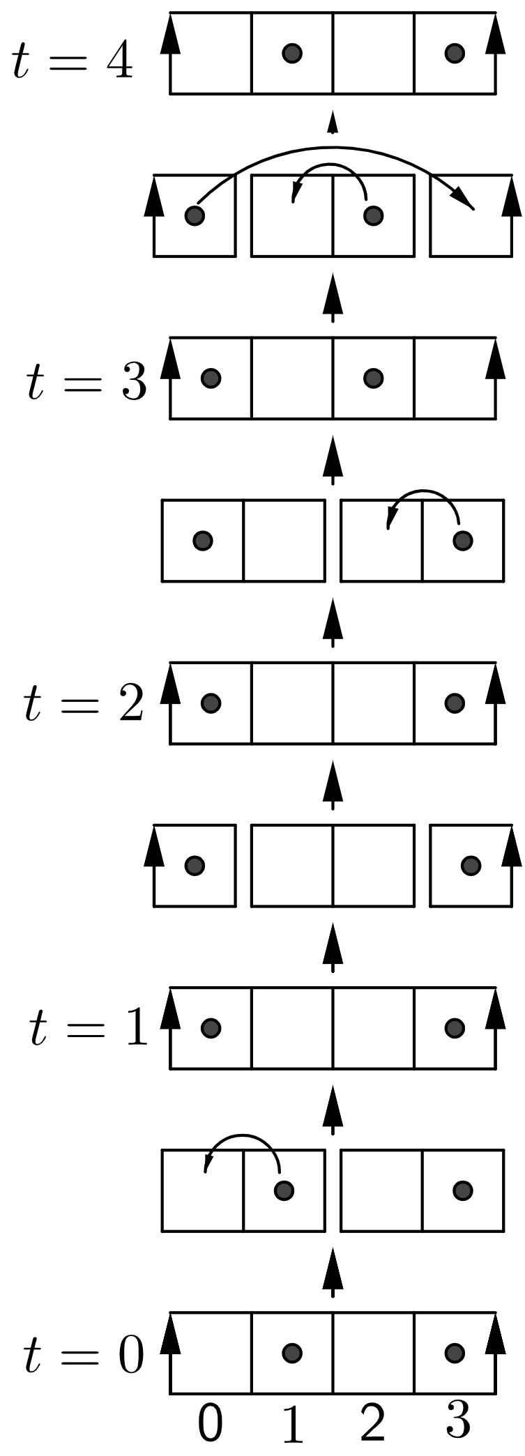
Figure 6: A realization

We conclude this section by restating Definition 9 informally in a self-contained way resembling exclusion process. (Cf. a different quantum exclusion process [1] defined by a continuous-time stochastic differential equation.)

Definition Sketch. (See Figure 6) Fix $T\in\mathbb{Z},\mu,\delta>0$ called half-period, particle mass, small imaginary mass respectively. Take a checkered stripe $1\times 2T$ closed in a ring. Enumerate the $2T$ squares by the numbers $0,\dots,2T-1$ consecutively.

Define a realization of the exclusion process inductively. At time $t=0$ some squares are occupied by identical particles, at most one per square.

At time $t=k$ decompose the stripe into $T$ rectangles $1\times 2$ so that squares $k$ and $k+1$ form a rectangle. In each rectangle with exactly $1$ particle, the particle is allowed to jump into the empty square of the same rectangle. In rectangles with $2$ or $0$ particles, nothing is changed.

Finally at time $t=2T$ it is requested that the particles occupy the same set of squares as at $t=0$. The resulting sequence of $2T$ configurations of particles at times $t=0,1,\dots,2T-1$ is a realization of the exclusion process.

A realization with a source at $(0,0)$ and a sink at $(x,t)\in\mathbb{Z}^{2}$ is defined analogously, only:

• at time $0$ before any jumps the square $0$ is empty, and a particle is added to the square;

• at time $t$ after all jumps the square $x$ is occupied, and the particle is removed from it.

To each realization $s$ (possibly with a source and a sink), assign a complex number $A(s)$ as follows. Start with $A(s)=(-1)^{n}$, where $n$ is the number of particles at time $0$ except the one added (at the source) and the one removed later (at the sink). For each moment $t=0,1,\dots 2T-1$ and each $1\times 2$ rectangle containing two particles at the moment $t$, multiply the current value of $A(s)$ by $-1$. For each moment $t=0,1,\dots 2T-1$ and each $1\times 2$ rectangle containing exactly one particle at the moment $t$, multiply the current value of $A(s)$ by

$$\begin{cases}1/\sqrt{1+\mu^{2}},&\text{if the particle jumps and $t$ is even};\\ -i\mu/\sqrt{1+\mu^{2}},&\text{if the particle does not jump and $t$ is even};\\ 1/\sqrt{1-\delta^{2}},&\text{if the particle jumps and $t$ is odd};\\ -\delta/\sqrt{1-\delta^{2}},&\text{if the particle does not jump and $t$ odd}.\end{cases}$$

The two-point function is then ${A}^{\mathrm{process}}(0,0\to x,t):=\frac{\sum\limits_{\begin{subarray}{c}\text{realizations $s$}\\ \text{with the source $(0,0)$ and the sink $(x,t)$}\end{subarray}}A(s)}{\sum\limits_{\begin{subarray}{c}\text{realizations $s$}\end{subarray}}A(s)}.$

Using Proposition 25, one can see that the two-point function actually equals the finite-lattice propagator; for instance, for $x,t$ even it equals $A(a_{0}\to f_{2};\mu/2,2,\delta,T)$. Notice that if we restrict to just realizations without particles at time $0$, drop space- and time-periodicity requirements, and take $\delta=0$, then the definition becomes equivalent to Definition 1.

Appendix B Wightman axioms

To put the new model in the general framework of quantum theory, we define the Hilbert space describing the states of the model along with the Hamiltonian and the field operators acting on this space. The definition is similar to (and simpler than) the continuum free spin $1/2$ field [7, §5.2], only we have unusual dispersion relation (3) and smaller number of spin components (coming from smaller spacetime dimension). Although the definition is self-contained, familiarity with the continuum analogue is desirable. We use notation $f^{*}$, $f^{\dagger}$, $\bar{f}$, $\langle f|g\rangle$ from [7, §1.1] (introduced below) unusual in mathematics but common in physics. For simplicity, we first perform the construction for the model with a fixed spatial size, then for the infinite lattice, and finally discuss which Wightman axioms of quantum field theory are satisfied.

Informal motivation

In quantum theory, a system is described by a Hilbert space encoding all possible states of the system. Examples of states of a free field (in a box of fixed spatial size) are: the vacuum state without any particles at all; the state with one particle of given momentum $p$; the state with two particles of momenta $p_{1}$ and $p_{2}$; the state with one particle of momentum $p$ and one anti-particle of momentum $q$; and so on. States of this kind actually form a basis of the Hilbert space. In general, a state is an arbitrary unit vector of the Hilbert space up to scalar multiples.

What quantum theory can compute is the expectation of observables such as the total energy of the system (the Hamiltonian) or charge density at a particular point. In general, an observable is a self-adjoint operator on the Hilbert space. The expectation of the observable in a given state equals the inner product of the state with its image under the operator.

Field operators are not observables but are building blocks for those. They are used to construct states such as the state with one right electron at position $x$ and time $t$, and useful functions such as the propagator.

Definition for fixed spatial size

Definition 10.

Fix $X\in\mathbb{Z}$ called lattice spatial size and $\varepsilon,m>0$. Assume $X>0$. Define $\widetilde{A}_{k}(x,t,m,\varepsilon,X)$ analogously to $\widetilde{A}_{k}(x,t,m,\varepsilon)$ (see Definition 2), only take the quotient

$$\faktor{\{\,(x,t)\in[0,X\varepsilon]\times\mathbb{R}:2x/\varepsilon,2t/\varepsilon,(x+t)/\varepsilon\in\mathbb{Z}\,\}}{\forall t\,(0,t)\sim(X\varepsilon,t).}$$

The momentum space is

$$\mathcal{P}_{X}:=\left\{\frac{2\pi k}{X\varepsilon}:-\frac{X}{2}<k\leq\frac{X}{2},k\in\mathbb{Z}\right\}.$$

Denote by $L_{2}(\mathcal{P}_{X})$ the Hilbert space with the finite orthonormal basis formed by the functions $\chi_{p}\colon\mathcal{P}_{X}\to\mathbb{C}$ equal to $1$ at a particular element $p\in\mathcal{P}_{X}$ and vanishing at all the other elements. Equip it with the natural inner product antilinear in the first argument. Let $\otimes$ and $\wedge$ be respectively the tensor and exterior product over $\mathbb{C}$. An empty exterior product of vectors (respectively, spaces) is set to be $1$ (respectively, $\mathbb{C}$).

The Hilbert space of $X$-periodic Feynman anticheckers is the $2^{2X}$-dimensional Hilbert space

$$\mathcal{H}_{X}:=\left(\bigoplus_{n=0}^{X}\bigwedge^{n}L_{2}\left(\mathcal{P}_{X}\right)\right)^{\otimes 2}.$$

It has an orthonormal basis formed by the vectors

$$\sqrt{n!l!}(\chi_{p_{1}}\wedge\dots\wedge\chi_{p_{n}})\otimes(\chi_{q_{1}}\wedge\dots\wedge\chi_{q_{l}})$$ (33)

for all integers $n,l$ from $0$ to $X$ and all $p_{1},\dots,p_{n},q_{1},\dots,q_{l}\in\mathcal{P}_{X}$ such that $p_{1}<\dots<p_{n}$ and $q_{1}<\dots<q_{l}$. (Physically, the vectors mean the states with $n$ electrons of momenta $p_{1},\dots,p_{n}$ and $l$ positrons of momenta $q_{1},\dots,q_{l}$.) The basis vector $1\in\mathbb{C}=\bigwedge^{0}L_{2}\left(\mathcal{P}_{X}\right)$ obtained for $n=l=0$ is the vacuum vector. It is denoted by $|0\rangle$. The dual vector is denoted by $\langle 0|\in\mathcal{H}_{X}^{*}$.

The Hamiltonian of $X$-periodic Feynman anticheckers is the linear operator on $\mathcal{H}_{X}$ such that all basis vectors (33) are eigenvectors with the eigenvalues (see notation (3))

$$\omega_{p_{1}}+\dots+\omega_{p_{n}}+\omega_{q_{1}}+\dots+\omega_{q_{l}}.$$

(Physically, $\omega_{p}$ is viewed as the energy of a particle with momentum $p$; hence the Hamiltonian eigenvalues mean total energy of the eigenstates.)

For $p\in\mathcal{P}_{X}$, the creation operators $a_{p}^{\dagger}$ and $b_{q}^{\dagger}$ of particles and antiparticles with momenta $p$ and $q$ respectively are the linear operators on $\mathcal{H}_{X}$ defined on basis vectors (33) by

$$a_{p}^{\dagger}\left(\sqrt{n!l!}(\chi_{p_{1}}\wedge\dots\wedge\chi_{p_{n}})\otimes(\chi_{q_{1}}\wedge\dots\wedge\chi_{q_{l}})\right) :=\sqrt{(n+1)!l!}(\chi_{p}\wedge\chi_{p_{1}}\wedge\dots\wedge\chi_{p_{n}})\otimes(\chi_{q_{1}}\wedge\dots\wedge\chi_{q_{l}}),$$

$$b_{q}^{\dagger}\left(\sqrt{n!l!}(\chi_{p_{1}}\wedge\dots\wedge\chi_{p_{n}})\otimes(\chi_{q_{1}}\wedge\dots\wedge\chi_{q_{l}})\right) :=(-1)^{n}\sqrt{n!(l+1)!}(\chi_{p_{1}}\wedge\dots\wedge\chi_{p_{n}})\otimes(\chi_{q}\wedge\chi_{q_{1}}\wedge\dots\wedge\chi_{q_{l}}).$$

Their adjoint operators are denoted by $a_{p}$ and $b_{q}$ respectively. For each $t\in\varepsilon\mathbb{Z}$ and $x\in\faktor{\varepsilon\mathbb{Z}}{X\varepsilon\mathbb{Z}}$ define the field operator $\psi_{X}(x,t)\colon\mathcal{H}_{X}\to\mathcal{H}_{X}\oplus\mathcal{H}_{X}$ by

$$\psi_{X}(x,t):=\frac{1}{\sqrt{X}}\sum_{p\in\mathcal{P}_{X}}\left(\begin{pmatrix}-i\cos(\alpha_{p}/2)\\ \sin(\alpha_{p}/2)\end{pmatrix}e^{ipx-i\omega_{p}t}a_{p}+\begin{pmatrix}i\cos(\alpha_{p}/2)\\ \sin(\alpha_{p}/2)\end{pmatrix}e^{i\omega_{p}t-ipx}b_{p}^{\dagger}\right),$$

where $\alpha_{p}\in[0,\pi]$ is determined by the condition $\cot\alpha_{p}=\frac{\sin(p\varepsilon)}{m\varepsilon}.$ (Informally, the field operator creates a positron or annihilates an electron at position $x$ and time $t$.)

The propagator is defined through field operators as follows. Denote by $\psi^{\dagger}_{X}(x,t)\colon\mathcal{H}_{X}\oplus\mathcal{H}_{X}\to\mathcal{H}_{X}$ the adjoint of the operator $\psi_{X}(x,t)$. Define the Dirac adjoint by $\bar{\psi}_{X}(x,t):=\psi_{X}^{\dagger}(x,t)\left(\begin{smallmatrix}0&-i\\ i&0\end{smallmatrix}\right)$. Define the time-ordered product

$$\mathrm{T}\psi_{X}(x,t)\bar{\psi}_{X}(0,0):=\begin{cases}\psi_{X}(x,t)\bar{\psi}_{X}(0,0),&\text{if }t\geq 0;\\ -\bar{\psi}_{X}(0,0)^{T}\psi_{X}(x,t)^{T},&\text{if }t<0.\end{cases}$$

The Feynman propagator for $X$-periodic Feynman anticheckers is $\langle 0|\mathrm{T}\psi_{X}(x,t)\bar{\psi}_{X}(0,0)|0\rangle$.

A direct checking using an analogue of Proposition 1 shows that the two constructions of the propagator are consistent: for each $x,t\in\varepsilon\mathbb{Z}$ and positive $X\in\mathbb{Z}$ the propagator for $X$-periodic Feynman anticheckers equals (cf. Proposition 27 below)

$$-i\begin{pmatrix}\widetilde{A}_{1}(-x,t,m,\varepsilon,X)&\widetilde{A}_{2}(x,t,m,\varepsilon,X)\\ -\widetilde{A}_{2}(-x,t,m,\varepsilon,X)&\widetilde{A}_{1}(x,t,m,\varepsilon,X)\end{pmatrix}.$$

Definition for the infinite lattice

Definition 11.

Denote by $L_{2}[a;b]$ the Hilbert space of square-integrable functions $[a;b]\to\mathbb{C}$ with respect to the Lebesque measure up to changing on a set of measure zero. Equip it with the inner product $\langle f|g\rangle:=\int_{[a;b]}f^{*}(p)g(p)\,dp$ antilinear in the first argument, where ^∗ denotes complex conjugation. Denote by $\bigoplus$, $\bigotimes$, and $\bigwedge$ the orthogonal direct sum, the tensor and exterior product of Hilbert spaces, that is, completions of the orthogonal direct sum, the tensor and exterior product of Hermitian spaces over $\mathbb{C}$.

Fix $\varepsilon,m>0$. The Hilbert space of Feynman anticheckers is the Hilbert space

$$\mathcal{H}:=\left(\bigoplus_{n=0}^{\infty}\bigwedge^{n}L_{2}\left[-\frac{\pi}{\varepsilon};\frac{\pi}{\varepsilon}\right]\right)^{\otimes 2}.$$

The vector $1\in\mathbb{C}=\bigwedge^{0}L_{2}\left[-\frac{\pi}{\varepsilon};\frac{\pi}{\varepsilon}\right]$ is denoted by $|0\rangle$. The dual vector is denoted by $\langle 0|\in\mathcal{H}^{*}$. Denote by $\mathcal{H}^{0}\subset\mathcal{H}$ the (incomplete) linear span of all $\bigwedge^{n}L_{2}\left[-\frac{\pi}{\varepsilon};\frac{\pi}{\varepsilon}\right]$ for $n=0,1,\dots$.

The Hamiltonian of Feynman anticheckers is the linear operator on $\mathcal{H}^{0}$ given by (see (3))

$$H(u_{1}\wedge\dots\wedge u_{n}\otimes v_{1}\wedge\dots\wedge v_{l}):=(\omega_{p}u_{1})\wedge\dots\wedge u_{n}\otimes v_{1}\wedge\dots\wedge v_{l}+\dots+u_{1}\wedge\dots\wedge u_{n}\otimes v_{1}\wedge\dots(\omega_{p}v_{l})$$

for all integers $n,l\geq 0$ and all $u_{1},\dots,u_{n},v_{1},\dots,v_{l}\in L_{2}\left[-\frac{\pi}{\varepsilon};\frac{\pi}{\varepsilon}\right]$, where $\omega_{p}$ is understood as a function in $p$. The evolution operator is the bounded linear operator on $\mathcal{H}$ given by

$$e^{-iHt}(u_{1}\wedge\dots\wedge u_{n}\otimes v_{1}\wedge\dots\wedge v_{l}):=(e^{-i\omega_{p}t}u_{1})\wedge\dots\wedge(e^{-i\omega_{p}t}u_{n})\otimes(e^{-i\omega_{p}t}v_{1})\wedge\dots\wedge(e^{-i\omega_{p}t}v_{l}).$$

The operators $P$ and $e^{-iPx}$ are defined analogously, only $\omega_{p}$ and $t$ are replaced by $p$ and $x$.

For $f\in L_{2}\left[-\frac{\pi}{\varepsilon};\frac{\pi}{\varepsilon}\right]$, the creation operators $a(f)^{\dagger}$ and $b(f)^{\dagger}$ of particles and antiparticles respectively with momentum distribution $f$ are the linear operators on $\mathcal{H}$ defined by

$$a(f)^{\dagger}(u\otimes v) :=\sqrt{n+1}\,(f\wedge u)\otimes v,$$

$$b(f)^{\dagger}(u\otimes v) :=(-1)^{n}\sqrt{l+1}\,u\otimes(f^{*}\wedge v)$$

for all $u\in\bigwedge^{n}L_{2}\left[-\frac{\pi}{\varepsilon};\frac{\pi}{\varepsilon}\right]$ and $v\in\bigwedge^{l}L_{2}\left[-\frac{\pi}{\varepsilon};\frac{\pi}{\varepsilon}\right]$. Their adjoint operators are denoted by $a(f)$ and $b(f)$ respectively. For each $x,t\in\varepsilon\mathbb{Z}$ define the field operator $\psi(x,t)\colon\mathcal{H}\to\mathcal{H}\oplus\mathcal{H}$ by

$$\psi(x,t):=\left(\begin{matrix}\psi_{1}(x,t)\\ \psi_{2}(x,t)\end{matrix}\right):=\left(\begin{matrix}a(f_{1,x,t})+b(f^{*}_{1,x,t})^{\dagger}\\ a(f_{2,x,t})+b(f^{*}_{2,x,t})^{\dagger}\end{matrix}\right),\quad\text{where}\quad\begin{aligned} f_{1,x,t}&=\sqrt{{\varepsilon}/{\pi}}\,i\cos(\alpha_{p}/2)e^{i\omega_{p}t-ipx},\\ f_{2,x,t}&=\sqrt{{\varepsilon}/{\pi}}\,\sin(\alpha_{p}/2)e^{i\omega_{p}t-ipx}.\end{aligned}$$

(The creation, annihilation, and field operators are bounded; see [7, (4.57)].) The Feynman propagator for Feynman anticheckers is defined through them analogously to Definition 10.

This construction of the propagator is consistent with the ones from Definitions 2, 3, and 9:

Proposition 27.

Let $\mathrm{T}\langle f_{k,x,t}|f_{l,0,0}\rangle:=\begin{cases}\langle f_{k,x,t}|f_{l,0,0}\rangle,&\mbox{if }t\geq 0;\\ -\langle f_{l,0,0}|f_{k,x,t}\rangle,&\mbox{if }t<0.\end{cases}$ Then for all $x,t\in\varepsilon\mathbb{Z}$ we get

$$\langle 0|\mathrm{T}\psi(x,t)\bar{\psi}(0,0)|0\rangle=i\,\mathrm{T}\begin{pmatrix}\langle f_{1,x,t}|f_{2,0,0}\rangle&-\langle f_{1,x,t}|f_{1,0,0}\rangle\\ \langle f_{2,x,t}|f_{2,0,0}\rangle&-\langle f_{2,x,t}|f_{1,0,0}\rangle\end{pmatrix}=-i\begin{pmatrix}\widetilde{A}_{1}(-x,t,m,\varepsilon)&\widetilde{A}_{2}(x,t,m,\varepsilon)\\ -\widetilde{A}_{2}(-x,t,m,\varepsilon)&\widetilde{A}_{1}(x,t,m,\varepsilon)\end{pmatrix}.$$

Proof.

Case 1: $t\geq 0$. By definition, for each $k,l\in\{1,2\}$ we have

$$\langle 0|\mathrm{T}\psi_{k}(x,t)\bar{\psi}_{l}(0,0)|0\rangle=\langle 0|\psi_{k}(x,t)\bar{\psi}_{l}(0,0)|0\rangle=-i(-1)^{l}\langle 0|\psi_{k}(x,t)\psi_{3-l}^{\dagger}(0,0)|0\rangle=\\ =-i(-1)^{l}\psi_{k}^{\dagger}(x,t)|0\rangle\cdot\psi_{3-l}^{\dagger}(0,0)|0\rangle=-i(-1)^{l}\langle f_{k,x,t}|f_{3-l,0,0}\rangle,$$

where $\cdot$ denotes the inner product in $\mathcal{H}$. The latter equality follows from

$$\psi_{k}^{\dagger}(x,t)|0\rangle =\left(a(f_{k,x,t})^{\dagger}+b(f^{*}_{k,x,t})\right)|0\rangle=f_{k,x,t}\otimes 1\in\bigwedge^{1}L_{2}\left[-\frac{\pi}{\varepsilon};\frac{\pi}{\varepsilon}\right]\otimes\bigwedge^{0}L_{2}\left[-\frac{\pi}{\varepsilon};\frac{\pi}{\varepsilon}\right],$$

where $b(f)|0\rangle=0$ because for each $u\in\bigwedge^{n}L_{2}\left[-\frac{\pi}{\varepsilon};\frac{\pi}{\varepsilon}\right]$ and $v\in\bigwedge^{l}L_{2}\left[-\frac{\pi}{\varepsilon};\frac{\pi}{\varepsilon}\right]$ we have

$$b(f)|0\rangle\cdot(u\otimes v)=|0\rangle\cdot b(f)^{\dagger}(u\otimes v)=|0\rangle\cdot(-1)^{n}\sqrt{l+1}\,u\otimes(f^{*}\wedge v)=0$$

by the condition $\bigwedge^{0}L_{2}\left[-\frac{\pi}{\varepsilon};\frac{\pi}{\varepsilon}\right]\otimes\bigwedge^{0}L_{2}\left[-\frac{\pi}{\varepsilon};\frac{\pi}{\varepsilon}\right]\perp\bigwedge^{n}L_{2}\left[-\frac{\pi}{\varepsilon};\frac{\pi}{\varepsilon}\right]\otimes\bigwedge^{l+1}L_{2}\left[-\frac{\pi}{\varepsilon};\frac{\pi}{\varepsilon}\right]$. Thus by the definitions of $f_{k,x,t}$, $\alpha_{p}$ and Proposition 1 we get

$$\langle 0|\mathrm{T}\psi(x,t)\bar{\psi}(0,0)|0\rangle=\frac{-i\varepsilon}{\pi}\int_{-\pi/\varepsilon}^{\pi/\varepsilon}\begin{pmatrix}i\,\cos(\alpha_{p}/2)\sin(\alpha_{p}/2)&\cos^{2}(\alpha_{p}/2)\\ -\sin^{2}(\alpha_{p}/2)&i\,\cos(\alpha_{p}/2)\sin(\alpha_{p}/2)\end{pmatrix}e^{ipx-i\omega_{p}t}\,dp=\\ =\frac{-i\varepsilon}{2\pi}\int\limits_{-\pi/\varepsilon}^{\pi/\varepsilon}\begin{pmatrix}\frac{im\varepsilon}{\sqrt{m^{2}\varepsilon^{2}+\sin^{2}p\varepsilon}}&1+\frac{\sin p\varepsilon}{\sqrt{m^{2}\varepsilon^{2}+\sin^{2}p\varepsilon}}\\ \frac{\sin p\varepsilon}{\sqrt{m^{2}\varepsilon^{2}+\sin^{2}p\varepsilon}}-1&\frac{im\varepsilon}{\sqrt{m^{2}\varepsilon^{2}+\sin^{2}p\varepsilon}}\end{pmatrix}e^{ipx-i\omega_{p}t}\,dp=-i\begin{pmatrix}\widetilde{A}_{1}(-x,t,m,\varepsilon)&\widetilde{A}_{2}(x,t,m,\varepsilon)\\ -\widetilde{A}_{2}(-x,t,m,\varepsilon)&\widetilde{A}_{1}(x,t,m,\varepsilon)\end{pmatrix}.$$

Case 2: $t<0$. An analogous computation shows that

$$\langle 0|\mathrm{T}\psi_{k}(x,t)\bar{\psi}_{l}(0,0)|0\rangle=i(-1)^{l}\psi_{3-l}(0,0)|0\rangle\cdot\psi_{k}(x,t)|0\rangle=i(-1)^{l}\langle f_{3-l,0,0}|f_{k,x,t}\rangle=\left(-i(-1)^{l}\langle f_{k,x,t}|f_{3-l,0,0}\rangle\right)^{*}.$$

Thus we get the same integral formula as in Case 1, only the whole expression is conjugated. The change of the variables $p\mapsto\pi/\varepsilon-p$ and Proposition 1 complete the proof. ∎

Formula (2) for the expected charge is consistent with the expression through field operators, which we briefly recall now (this paragraph is addressed to specialists). Under notation from [7, §6.4], $:\!\psi^{\dagger}(x,t)\psi(x,t)\!:$ is the charge density operator for the spin-$1/2$ field [21, (3.113)]. Thus the expected charge density in the state $\psi_{2}^{\dagger}(0,0)|0\rangle$ (meaning one right electron at the origin) is

$$\langle 0|\psi_{2}(0,0):\!\psi^{\dagger}(x,t)\psi(x,t)\!:\psi_{2}^{\dagger}(0,0)|0\rangle=\left|\langle 0|\psi^{\dagger}(x,t)\psi_{2}(0,0)|0\rangle\right|^{2}=|\widetilde{A}_{1}\left(x,t,m,\varepsilon\right)|^{2}+|\widetilde{A}_{2}\left(x,t,m,\varepsilon\right)|^{2},$$

which coincides with (2) up to normalization. Here the first equality can be deduced, for instance, from a version of Wick’s theorem [7, (6.42)], and the second one — from Proposition 27.

Wightman axioms

The continuum limit of the new model is the well-known free spin-$1/2$ quantum field theory which of course satisfies Wightman axioms [7, §5.5]. One cannot expect the discrete model to satisfy all the axioms before passing to the limit because they are strongly tied to continuum spacetime and Lorentz transformations. Remarkably, some of them still hold on the lattice.

Proposition 28 (Checking of Wightman axioms).

The objects introduced in Definition 11 satisfy the following conditions:

axiom 1:

$\psi_{k}(x,t)$ is a bounded linear operator on $\mathcal{H}$ for each $(x,t)\in\varepsilon\mathbb{Z}^{2}$ and $k\in\{1,2\}$;

axiom 2:

$|0\rangle$ is the unique up to proportionality vector in $\mathcal{H}$ such that $e^{iH\varepsilon}|0\rangle=e^{iP\varepsilon}|0\rangle=|0\rangle$;

axiom 3:

the vectors $\psi_{k_{1}}(x_{1},t_{1})\dots\psi_{k_{l}}(x_{l},t_{l})\psi^{\dagger}_{k_{l+1}}(x_{l+1},t_{l+1})\dots\psi^{\dagger}_{k_{l+n}}(x_{l+n},t_{l+n})|0\rangle$ for all $0\leq n,l\in\mathbb{Z}$, $k_{j}\in\{1,2\}$, $(x_{j},t_{j})\in\varepsilon\mathbb{Z}^{2}$ span a dense linear subspace in $\mathcal{H}$;

axiom 4 (weakened):

$e^{biH-aiP}\psi_{k}(x,t)e^{aiP-biH}=\psi_{k}(x+a,t+b)$ for each $(a,b)\in\varepsilon\mathbb{Z}^{2}$;

axiom 5 (weakened):

$H\geq 0$ and $H^{2}-(1-\omega_{0}\varepsilon/\pi)^{2}P^{2}\geq 0$;

axiom 6:

$[\psi_{k}(x,t),\psi_{k^{\prime}}(x^{\prime},t^{\prime})]_{+}=[\psi_{k}(x,t),\psi^{\dagger}_{k^{\prime}}(x^{\prime},t^{\prime})]_{+}=[\psi^{\dagger}_{k}(x,t),\psi^{\dagger}_{k^{\prime}}(x^{\prime},t^{\prime})]_{+}=0$ for all $k,k^{\prime}\in\{1,2\}$ and $(x,t),(x^{\prime},t^{\prime})\in\varepsilon\mathbb{Z}^{2}$ such that $|x-x^{\prime}|>|t-t^{\prime}|$, where $[a,b]_{+}:=ab+ba$.

Here Axiom 1 is weaker than the continuum one in the sense that the field operators are defined only on the lattice, but stronger in the sense that they are genuine bounded operators rather than distributions. The vectors in Axiom 3 mean states with electrons at the points $(x_{l+1},t_{l+1}),\dots,(x_{l+n},t_{l+n})$ and positrons at the points $(x_{1},t_{1}),\dots,(x_{l},t_{l})$. Axiom 4 is much weaker than the continuum one, which involves general Lorentz transformations. On the lattice, only translations remain, because (almost all) the other Lorentz transformations do not preserve the lattice. Axiom 5 in continuum theory asserts that $H\geq 0$ and $H^{2}-P^{2}\geq 0$, i.e. the energy is positive in any frame of reference. The inequality $H^{2}-P^{2}\geq 0$ is violated on the lattice (but this does not mean negative energy because Lorentz transformations do not preserve the lattice). The weakened Axiom 5 shows that it still holds ‘‘in the continuum limit’’. Axiom 6 is equivalent to vanishing of the real part of the Feynman propagator outside the light cone; this is obvious in the original Feynman model but nontrivial in the new one.

Proof.

Axioms 1 and 2 hold by definition; recall that the operators are bounded by [7, (4.57)]. Axiom 3 holds because linear span of the functions $(\psi_{1}(x,0)+\psi_{2}(x,0))|0\rangle=i\sqrt{\varepsilon/\pi}\,e^{-i\alpha_{p}/2-ipx}$, where $x$ runs through $\varepsilon\mathbb{Z}$, is dense in $L_{2}\left[-\frac{\pi}{\varepsilon};\frac{\pi}{\varepsilon}\right]$. Axiom 4 is checked directly. Axiom 5 follows from the inequality $\omega_{p}\geq|p|(1-\omega_{0}\varepsilon/\pi)$.

To check Axiom 6, recall that all the anticommutators of the operators $a(f),a(f)^{\dagger},b(f),b(f)^{\dagger}$ vanish except $[a(f),a(g)^{\dagger}]_{+}=[b(f^{*}),b(g^{*})^{\dagger}]_{+}=\langle f|g\rangle I$ [7, (4.56) and p.96]. This immediately implies that $[\psi_{k}(x,t),\psi_{k^{\prime}}(x^{\prime},t^{\prime})]_{+}=[\psi^{\dagger}_{k}(x,t),\psi^{\dagger}_{k^{\prime}}(x^{\prime},t^{\prime})]_{+}=0$. Finally, by Proposition 27, Theorem 1, and Definition 1 for $|x-x^{\prime}|>|t-t^{\prime}|$ we have

$$[\psi_{k}(x,t),\psi^{\dagger}_{k^{\prime}}(x^{\prime},t^{\prime})]_{+}=[a(f_{k,x,t}),a(f_{k^{\prime},x^{\prime},t^{\prime}})^{\dagger}]_{+}+[b(f^{*}_{k,x,t})^{\dagger},b(f^{*}_{k^{\prime},x^{\prime},t^{\prime}})]_{+}=\\ =\langle f_{k,x,t}|f_{k^{\prime},x^{\prime},t^{\prime}}\rangle I+\langle f_{k^{\prime},x^{\prime},t^{\prime}}|f_{k,x,t}\rangle I=2I\,\mathrm{Re}\langle f_{k,x-x^{\prime},t-t^{\prime}}|f_{k^{\prime},0,0}\rangle=0.\\[-42.67912pt]$$

∎

Acknowledgements

The authors are grateful to M. Drmota and F. Kuyanov for useful discussions.

Mikhail Skopenkov
King Abdullah University of Science and Technology and
HSE University (Faculty of Mathematics) and
Institute for Information Transmission Problems, Russian Academy of Sciences
mikhail.skopenkov @ gmail$\cdot$com  https://users.mccme.ru/mskopenkov/

Alexey Ustinov
HSE University (Faculty of Computer Science) and
Khabarovsk Division of the Institute for Applied Mathematics,
Far-Eastern Branch, Russian Academy of Sciences, Russia
Ustinov.Alexey @ gmail$\cdot$com  http://iam.khv.ru/staff/Ustinov.php

References

- [1] M. Bauer, D. Bernard, T. Jin, Stochastic dissipative quantum spin chains (i): Quantum fluctuating discrete hydrodynamics, SciPost Phys. 3, 033 (2017).
- [2] C.M. Bender, L.R. Mead, K.A. Milton, Discrete time quantum mechanics, Computers Math. Appl. 28:10-12 (1994), 279-317.
- [3] C.M. Bender, K.A. Milton, D.H. Sharp, Gauge invariance and the finite-element solution of the Schwinger model, Phys. Rev. D 31 (1985), 383; Erratum Phys. Rev. D 32 (1985), 1593.
- [4] R.P. Feynman, QED: The strange theory of light and matter. Princeton University Press, 2006.
- [5] R.P. Feynman, A.R. Hibbs, Quantum mechanics and path integrals, New York, McGraw-Hill, 1965.
- [6] S.R. Finch, Mathematical constants, Cambridge University Press, 2003.
- [7] G.B. Folland, Quantum field theory. A tourist guide for mathematicians, Math.Surveys & Monographs 149, AMS, 2008.
- [8] B.Z. Foster, T. Jacobson, Spin on a 4D Feynman Checkerboard, Int. J. Theor. Phys. 56 (2017), 129–144.
- [9] J. Glimm, A. Jaffe, Quantum physics: a functional integral point of view, Springer Science & Business Media, 2012.
- [10] I.S. Gradstein, I.M. Ryzhik, Tables of integrals, sums, series and products, 4th ed., Moscow, Fizmatgiz, 1963, 1100 pp. (in Russian).
- [11] M.N. Huxley, Area, lattice points, and exponential sums, The Clarendon Press, 1996.
- [12] T. Jacobson, Feynman’s checkerboard and other games. In: N. Sanchez (eds) Non-linear equations in classical and quantum field theory. Lect. Notes in Phys., 226, Springer, Berlin, Heidelberg, 1985.
- [13] J. Kempe, Quantum random walks: an introductory overview, Contemp. Phys. 50:1 (2009), 339-359.
- [14] R. Kenyon, The Laplacian and Dirac operators on critical planar graphs, Invent. Math. 150 (2002), 409–439.
- [15] N. Konno, Quantum walks, Sugaku Expositions 33:2 (2020), 135–158.
- [16] F. Kuyanov, A. Slizkov, Feynman checkers: number-theoretic properties, preprint, 2022.
- [17] L. Levine, Algebraic Combinatorics, Lecture 18, http://pi.math.cornell.edu/~levine/18.312/alg-comb-lecture-18.pdf
- [18] J. Maldacena, The symmetry and simplicity of the laws of physics and the Higgs boson, Europ. J. Phys. 37:1 (2016).
- [19] I. Novikov, Feynman checkers: the probability to find an electron vanishes nowhere inside the light cone, Rev. Math. Phys. (2022), to appear. arXiv:2010.05088.
- [20] F. Ozhegov, Feynman checkers: external electromagnetic field and asymptotic properties, preprint (2022).
- [21] M.E. Peskin, D.V. Schroeder, An introduction to quantum field theory, Westview Press, Boulder, 1995.
- [22] H.J. Rothe, Lattice gauge theories: an introduction, World Scientific Publishing Company, 2012. https://library.oapen.org/bitstream/handle/20.500.12657/50492/9789814365871.pdf?sequence=1
- [23] S.S. Schweber, Feynman and the visualization of space-time processes, Rev. Mod. Phys. 58:2 (1986), 449–511.
- [24] M. Skopenkov, A. Ustinov, Feynman checkers: towards algorithmic quantum theory, Russian Math. Surveys 77:3(465) (2022), 73–160. arXiv:2007.12879.
- [25] M. Skopenkov, A. Ustinov, Feynman anticheckers: auxiliary computations. https://users.mccme.ru/mskopenkov/skopenkov-pdf/anticheckers-auxiliary-computations.nb. Last accessed 29.04.2022.
- [26] S. Smirnov, Conformal invariance in random cluster models. I. Holmorphic fermions in the Ising model, Ann. Math. 2nd Ser. 172:2 (2010), 1435–1467.
- [27] G. Szegö, Orthogonal polynomials, Colloquium Publications XXIII, American Math. Society, 1939.
- [28] S.E. Venegas-Andraca, Quantum walks: a comprehensive review, Quantum Inf. Process. 11 (2012), 1015–1106.
- [29] A. Zee, Quantum field theory in a nutshell, 2nd ed., Princeton University Press, Princeton, New Jersey (2010), 576 pp.
- [30] A. Zorich, Calculus, Vol.2, Fazis, 1997.