Local Wind Regime Induced by Giant Linear Dunes: Comparison of ERA5-Land Reanalysis with Surface Measurements

Abstract

Emergence and growth of sand dunes results from the dynamic interaction between topography, wind flow and sediment transport. While feedbacks between these variables are well studied at the scale of a single and relatively small dune, the average effect of a periodic large-scale dune pattern on atmospheric flows remains poorly constrained, due to a pressing lack of data in major sand seas. Here, we compare local measurements of surface winds to the predictions of the ERA5-Land climate reanalysis at four locations in Namibia, both within and outside the giant linear dune field of the Namib Sand Sea. In the desert plains to the north of the sand sea, observations and predictions agree well. This is also the case in the interdune areas of the sand sea during the day. During the night, however, an additional wind component aligned with the giant dune orientation is measured, in contrast to the easterly wind predicted by the ERA5-Land reanalysis. For the given dune orientation and measured wind regime, we link the observed wind deviation (over 50°) to the daily cycle of the turbulent atmospheric boundary layer. During the night, a shallow boundary layer induces a flow confinement above the giant dunes, resulting in large flow deviations, especially for the slower easterly winds. During the day, the feedback of the giant dunes on the atmospheric flow is much weaker due to the thicker boundary layer and higher wind speeds. Finally, we propose that the confinement mechanism and the associated wind deflections induced by giant dunes could explain the development of smaller-scale secondary dunes, which elongate obliquely in the interdune areas of the primary dune pattern.

An edited version of this paper was published by Springer Nature: Gadal, C., Delorme, P., Narteau, C. et al. Local Wind Regime Induced by Giant Linear Dunes: Comparison of ERA5-Land Reanalysis with Surface Measurements. Boundary-Layer Meteorol (2022). https://doi.org/10.1007/s10546-022-00733-6 .

1 Introduction

The description of turbulent flows over complex topography is relevant for a large variety of different environmental systems (Sherman 1978; Walmsley et al. 1982; Baines 1995; Wood 2000; Venditti et al. 2013; Finnigan et al. 2020). For example, the flow over hills is of primary interest for wind power, meteorological and air pollution phenomena (Taylor et al. 1987). The properties of these flows are also key to the understanding of geophysical phenomena, including the formation of wind-driven waves on the ocean surface (Sullivan and McWilliams 2010), dissolution bedforms (Claudin et al. 2017; Guérin et al. 2020), or sedimentary ripples and dunes (Bagnold 1941; Charru et al. 2013; Courrech du Pont 2015). Importantly, the troposphere presents a vertical structure, with a lower convective boundary layer, of typical kilometer-scale thickness, capped by a stably stratified region (Stull 1988). The largest topographic obstacles, such as mountains, can therefore interact with this upper region and lead to internal wave generation or significant wind disturbances, such as lee-side downslope winds (Durran 1990).

Compared to hills and mountains, aeolian sand dunes offer idealized elevation profiles for the study of atmospheric turbulent flow over topographies, due to their smooth shape, free of canopies. Besides, dunes provide a rather wide range of scales, from decameters to kilometers, and very often come in a fairly regular pattern, which further simplifies the flow structure analysis. Past studies have highlighted two important topographic feedbacks on the wind flow close to the dune/hill surface. First is the effect on wind speed, with documented flow acceleration on upwind slopes (Weaver and Wiggs 2011) and deceleration on downwind slopes (Baddock et al. 2007), where the speed-up factor is essentially proportional to the obstacle aspect ratio (Jackson and Hunt 1975). Under multidirectional wind regimes with frequent wind reversals, this speed-up effect induces large differences in the amplitude and orientation of the resultant sediment transport between flat sand beds and the dune crests (Zhang et al. 2014; Rozier et al. 2019; Gao et al. 2021). In addition, the position of maximum velocity is typically shifted upwind of the obstacle crest (Jackson and Hunt 1975; Claudin et al. 2013). This behaviour has been theoretically predicted by means of asymptotic analysis of a neutrally stratified boundary-layer flow over an obstacle of vanishing aspect ratio (Jackson and Hunt 1975; Mason and Sykes 1979; Sykes 1980; Hunt et al. 1988; Belcher and Hunt 1998; Kroy et al. 2002). Experiments in flumes (Zilker et al. 1977; Zilker and Hanratty 1979; Frederick and Hanratty 1988; Poggi et al. 2007; Bristow et al. 2022), in wind tunnels (Gong and Ibbetson 1989; Finnigan et al. 1990; Gong et al. 1996) and in field conditions at all scales (Taylor and Teunissen 1987; Claudin et al. 2013; Fernando et al. 2019; Lü et al. 2021), have also documented this effect. Interestingly, a similar behaviour exists for the pressure perturbation, but with a slight downwind shift for the pressure minimum (Claudin et al. 2021).

The second effect, much less studied, is the flow deflection that occurs when the incident wind direction is not perpendicular to the ridge crest. While predicted to be small (less than $10^{\circ}$) in the linear regime valid for shallow topography (Gadal et al. 2019), significant flow steering has been reported in the field on the downwind side of steep enough obstacles, such as well-developed sand dunes (Tsoar and Yaalon 1983; Sweet and Kocurek 1990; Walker and Nickling 2002; Smith et al. 2017) and in particular coastal foredunes (e.g. Hunter et al. 1983; Rasmussen 1989; Walker et al. 2006, 2009; Hesp et al. 2015; Walker et al. 2017; de Winter et al. 2020), mountain ranges (Kim et al. 2000; Lewis et al. 2008; Fernando et al. 2019), and valley topographies (Wiggs et al. 2002; Garvey et al. 2005).

Wind measurements over sand dunes have been mainly performed over small bedforms, typically a few meters high (corresponding to several tens of meters long) (e.g. Mulligan 1988; Hesp et al. 1989; Lancaster et al. 1996; McKenna Neuman et al. 1997; Sauermann et al. 2003; Andreotti et al. 2002; Walker and Nickling 2002; Weaver and Wiggs 2011). For practical reasons, fewer studies have performed similar measurements on giant dunes (Havholm and Kocurek 1988), with kilometer-scale wavelengths and heights of tens of meters. However, such large dunes provide a choice configuration for the study of turbulent flows over a complex topography. First, one expects larger wind disturbances for larger obstacles. Secondly, their large size can make them interact with the vertical structure of the atmosphere (Andreotti et al. 2009). Third, they usually form large patterns in sand seas and thus behave as rather clean periodic perturbations, in contrast with isolated dunes. Finally, because the morphodynamics of aeolian bedforms is strongly dependent on the local wind regime (Livingstone and Warren 2019), one can expect to see the consequences of windflow disturbance by large dunes on neighbouring small dunes (Brookfield 1977; Ewing et al. 2006). A similar effect is observed on the properties of impact ripple patterns due to the presence of dunes (Howard 1977; Hood et al. 2021).

Atmospheric flows have been much studied at the desert-scale with climate reanalyses based on global atmospheric models (Blumberg and Greeley 1996; Livingstone et al. 2010; Ashkenazy et al. 2012; Jolivet et al. 2021; Hu et al. 2021; Gunn et al. 2021), such as ERA-40, ERA-Interim or ERA5 (Uppala et al. 2005; Dee et al. 2011; Hersbach et al. 2020). However, the spatial resolution of these reanalyses (tens of kilometers) implies average quantities that do not resolve the smaller scales of interest, which range from individual dunes to small mountains (Livingstone et al. 2010). Recently, the release of ERA5-Land has partly resolved this limitation by providing up to 70 years of hourly wind predictions at a $9$ km spatial resolution (Muñoz-Sabater et al. 2021). However, its validity remains to be studied, especially in remote desert areas where assimilation of measured data is very low.

In this work, we compare local wind speeds and directions measured by meteorological stations at four different locations inside and north of the giant linear dune field of the Namib sand sea to the regional predictions of the ERA5-Land climate reanalysis. Where the meteorological stations are surrounded by a relatively flat environment, we show that local measurements and regional predictions agree well. The agreement is also good in the interdune areas of the sand sea, except for some weak winds blowing at night, which exhibit an additional component aligned with the giant dune orientation. These winds are not predicted by the ERA5-Land reanalysis (Sect. 2). Further, we are able to link the magnitude of these differences to the circadian cycle of the atmospheric boundary layer (Sect. 3). Finally, we draw implications for the wind disturbances on smaller-scale dunes (Sect. 4), suggesting a possible origin for crossing dunes, a distinctive secondary dune form observed in the Namib and other sand seas.

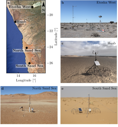
Figure 1: Studied field sites. a Location of the different sites in Namibia. b-e: Photographs of the meteorological stations.

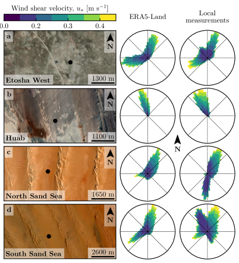
Figure 2: Wind data used in this study. Satellite images of the different environments (Google-Earth, Maxar Technologies, CNES/Airbus) are shown on the left. The black dots show the location of the wind measurements stations. On the right of the photos, the corresponding wind roses representing the data from the ERA5-Land climate reanalysis and the local wind stations are displayed. Note: the graphical convention for the wind roses is that the bars show the direction towards which the wind blows (see color bar for velocity scale).

2 Wind Regimes Across The Namib Sand Sea

We measured the wind regime at four different locations in Namibia, representative of various arid environments across the Namib desert (Figs. 1 and 2). The Etosha West station was located at the Adamax waterhole to the west of Etosha Pan in northern Namibia, in a sparsely vegetated area. The Huab station was near the coast on a hyper-arid flat gravel plain lying north of the ephemeral Huab river. Here, barchan dunes up to a few meters in height develop from the sediment blowing out of the river valley (Nield et al. 2017; Hesp and Hastings 1998). These two stations were both located in relatively flat environments. In contrast, the North Sand Sea and South Sand Sea stations were located in the interdunes between linear dunes with kilometer-scale wavelengths, hectometer-scale heights and superimposed patterns. In this section, we describe and compare winds from local measurements and climate reanalysis predictions.

2.1 Wind and Elevation Data

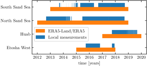
Figure S1: Gantt chart representing the valid time steps for the two data sets, for all stations.

At each meteorological station (Fig. 1), wind speed and direction were sampled every 10 minutes using cup anemometers (Vector Instruments A100-LK) and wind vanes (Vector Instruments W200-P) at a single height, which was between 2 m and 3 m depending on the station. The available period of measurements at each station ranged from 1 to 5 discontinuous years distributed between 2012 and 2020 (Online Resource Fig. S1). We checked that at least one complete seasonal cycle was available for each station. Regional winds were extracted at the same locations and periods from the ERA5-Land dataset, which is a replay at a smaller spatial resolution of ERA5, the latest climate reanalysis from the ECMWF (Hersbach et al. 2020; Muñoz-Sabater et al. 2021). This dataset provided hourly predictions of the 10-m wind velocity and direction at a spatial resolution of $0.1^{\circ}\times 0.1^{\circ}$ ($\simeq 9~{}\textup{km}$ in Namibia).

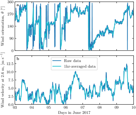
Figure S2: Local wind measurements: comparison between raw (blue) and hourly-averaged (light blue) data from South Sand Sea station. a: wind direction. b: wind velocity at height $2.6$ m.

To enable direct comparison, the local wind measurements were averaged into 1-hr bins centered on the temporal scale of the ERA5-Land estimates (Online Resource Fig. S2). As the wind velocities of both datasets were provided at different heights, we converted them into shear velocities $u_{*}$ (Online Resource section 1), characteristic of the turbulent wind profile. Wind roses in Fig. 2 show the resulting wind data.

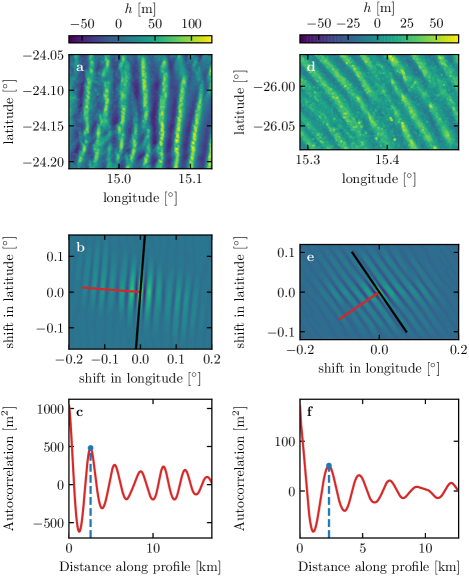
Figure S4: Analysis of the DEMs of the North Sand Sea (left column – panels a, b, c) and South Sand Sea (right column – panels d, e, f) stations. a–d: Bed elevation detrended by a fitted second order polynomial base-line. b–e: Autocorrelation matrix shown in color scale. The black line shows the detected dune orientation, and the red line represents the autocorrelation profile along which the dune wavelength is calculated, displayed in c–f. The blue lines and dots show the first peak of the autocorrelation profile, whose abscissa gives the characteristic wavelength of the dune pattern.

Dune properties were computed using autocorrelation on the 30-m Digital Elevation Models (DEMs) of the shuttle radar topography mission (Farr et al. 2007). For the North and South Sand Sea stations, we obtain, respectively, orientations of $85^{\circ}$ and $125^{\circ}$ with respect to the North, wavelengths of $2.6~{}\textup{km}$ and $2.3~{}\textup{km}$ and amplitudes (or half-heights) of $45~{}\textup{m}$ and $20~{}\textup{m}$ (Online Resource Fig. S4 for more details). This agrees with direct measurements made on site.

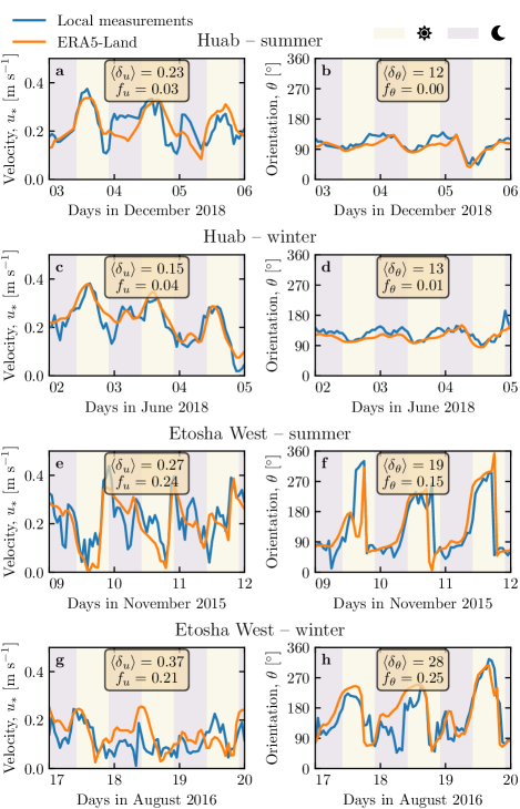
Figure 3: Temporal comparison between the wind data coming from the ERA5-Land climate reanalysis (orange lines) and from the local measurements (blue lines). Coloured swathes indicate day (between 10.00 UTC and 22.00 UTC) and night (before 10.00 UTC or after 22.00 UTC). Numbers in legends indicate the average flow deflection $\delta_{\theta}$ and relative wind modulation $\delta_{u}$ over the displayed period (see Sect. 3.2 for their definitions), as well as the percentage $f_{\theta}$ and $f_{u}$ of occurrence of extreme events ($\delta_{\theta}>50^{\circ}$, $|\delta_{u}|>0.6$). a,b: Huab station in summer. b,c: Huab station in winter. d,e: Etosha West station in summer. f,g: Etosha West station in winter. Time series of the two other stations are shown in Fig. 5.

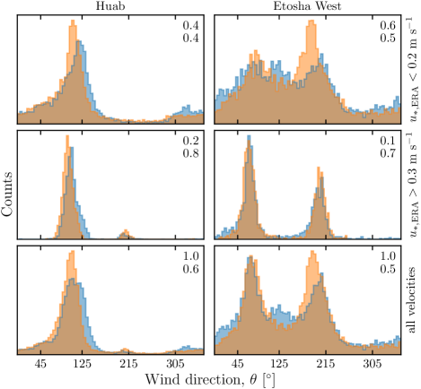
Figure 4: Distributions of wind direction at Huab and Etosha West stations for the ERA5-Land climate reanalysis (orange) and the local measurements (blue). In each subplot, both distributions are plotted from the same time steps, selected for different ranges of the wind wind velocity (rows) in the ERA5-Land dataset. The numbers at the upper right corners give the percentage of time steps selected in each sub-range (top), as well as the percentage of them corresponding to the day – defined between 10.00 UTC and 22.00 UTC (bottom).

2.2 Comparison of Local and Regional Winds

The measured and predicted wind regimes are shown in Fig. 2. In the Namib, the regional wind patterns are essentially controlled by the sea breeze, resulting in strong northward components (sometimes slightly deviated by the large scale topography) present in all regional wind roses (Lancaster 1985). These daytime winds are dominant during the period October–March (Fig. 3f and Online Resource Fig. 4f). During April–September, an additional (and often nocturnal) easterly component can also be recorded, induced by the combination of katabatic winds forming in the mountains, and infrequent ‘berg’ winds, which are responsible for the high wind velocities observed (Lancaster et al. 1984). The frequency of these easterly components decreases from inland to the coast. As a result, bidirectional wind regimes within the Namib Sand Sea and at the west Etosha site (Fig. 2a,c and d) and a unidirectional wind regime on the coast at the outlet of the Huab River (Fig. 2b) are observed.

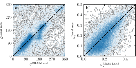
Figure S5: Statistical comparison of the wind orientation (a) and velocity (b) between the ERA5-Land dataset and the local measurements for the Huab and Etosha West stations. Data point clustering around identity lines (dashed and black) provide evidence for agreement of the two sets.

In the case of the Etosha West and Huab stations, the time series of wind speed and direction from the regional predictions quantitatively match those corresponding to the local measurements (Figs. 3,  4 and Online Resource Fig. S5). For the North Sand Sea and South Sand Sea stations within the giant linear dune field, we observe that this agreement is also good, but limited to the October-March time period (Fig. 4a, b and e, f). However, the field-measured wind roses exhibit additional wind components aligned with the dune orientation, as evidenced on the satellite images (Fig. 2c and d).

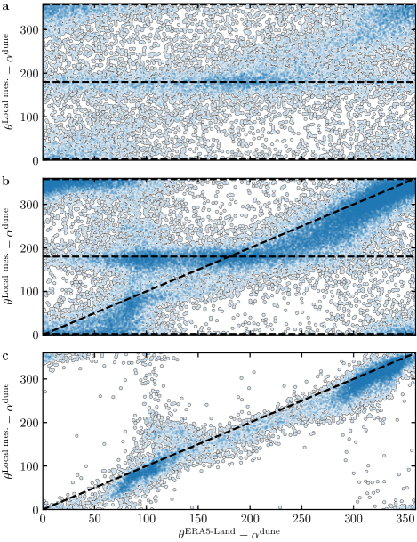
Figure S6: Statistical comparison of the wind orientation between the ERA5-Land dataset and the local measurements for the South Sand Sea and North Sand Sea stations, for different velocity ranges. a: $u_{*}^{\textup{ERA5-Land}}<0.1~{}\textup{m}~{}\textup{s}^{-1}$. b: $0.1<u_{*}^{\textup{ERA5-Land}}\leq 0.25~{}\textup{m}~{}\textup{s}^{-1}$. c: $u_{*}^{\textup{ERA5-Land}}\geq 0.25~{}\textup{m}~{}\textup{s}^{-1}$. The measured dune orientations are subtracted to the wind orientation, which allows us to plot both stations on the same graph. Black dashed lines indicate locally measured orientations aligned with the dune crests (here $0^{\circ}$, $180^{\circ}$ and $360^{\circ}$ – panels a, b), as well as the identity lines (panels b, c).

More precisely, during the April–September period, the local and regional winds in the interdune match during daytime only, i.e when the southerly/southwesterly sea breeze dominates (Figs. 5c,d,g,h and 6). In the late afternoon and during the night, when the easterly ‘berg’ and katabatic winds blow, measurements and predictions differ. In this case, the angular wind distribution of the local measurements exhibits two additional modes corresponding to reversing winds aligned with the dune orientation (purple frame in Fig. 6, Online Resource Fig. S6). This deviation is also associated with a general attenuation of the wind strength (Online Resource Fig. S7). Remarkably, all these figures show that these wind reorientation and attenuation processes occur only at low velocities of the regional wind, typically for $u_{*}^{\textup{ERA5-Land}}\lesssim 0.2~{}\textrm{m}~{}\textrm{s}^{-1}$. For shear velocities larger than $u_{*}^{\textup{ERA5-Land}}\simeq 0.3~{}\textrm{m}~{}\textrm{s}^{-1}$, the wind reorientation is not apparent. Finally, for intermediate shear velocities, both situations of wind flow reoriented along the dune crest and not reoriented can be successively observed (Online Resource Fig. S6). Importantly, these values are not precise thresholds (and certainly not related to the threshold for sediment transport), but indicative of a crossover between regimes, whose physical interpretation is discussed in the next section.

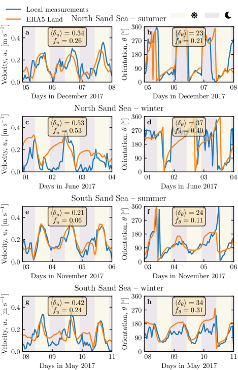
Figure 5: Same as Fig. 3 for North Sand Sea station in summer (a,b), North Sand Sea station in winter (b,c), South Sand Sea station in summer (d,e) and South Sand Sea station in winter (f,g).

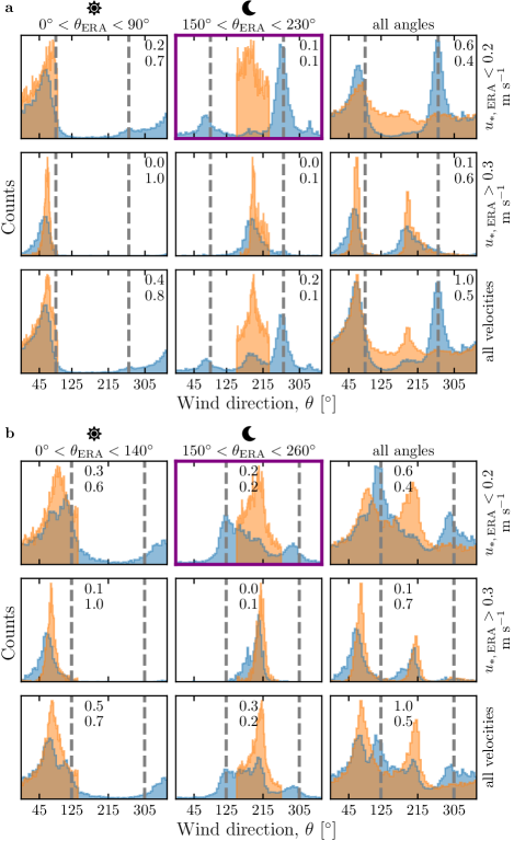
Figure 6: Same as Fig. 4 but for North Sand Sea (a) and South Sand Sea (b) stations. Here, subplots correspond to different ranges for the wind direction (columns) and wind velocity (rows) of the ERA5-Land dataset. The grey vertical dashed lines indicate the main dune orientation. In contrast with observations at the Huab and Etosha West stations (Fig. 4), histograms do not match well at low wind velocities, and the purple frame highlights the regime (low wind velocities, nocturnal easterly wind) in which the data from both datasets differ most.

3 Influence of Wind Speed and Circadian Cycle on the Atmospheric Boundary Layer

The wind deflection induced by dunes has previously been related to the incident angle between wind direction and crest orientation, with a maximum deflection evident for incident angles between $30^{\circ}$ and $70^{\circ}$ (Walker et al. 2009; Hesp et al. 2015). In the data analysed here, the most deflected wind at both the North and South Sand Sea stations is seen to be where the incident angle is perpendicular to the giant dunes (Figs. 2 and 6). It therefore appears that in our case, the incident wind angle is not the dominant control on maximum wind deflection. Further, and as shown in Fig. 6, winds of high and low velocities show contrasting behaviour in characteristics of deflection. This suggests a change in hydrodynamical regime between the winds. In this section, we discuss the relevant parameters associated with the dynamical mechanisms that govern the interactions between the atmospheric boundary layer flow and giant dune topographies. This analysis allows us to provide a physics-based interpretation of our measured wind data.

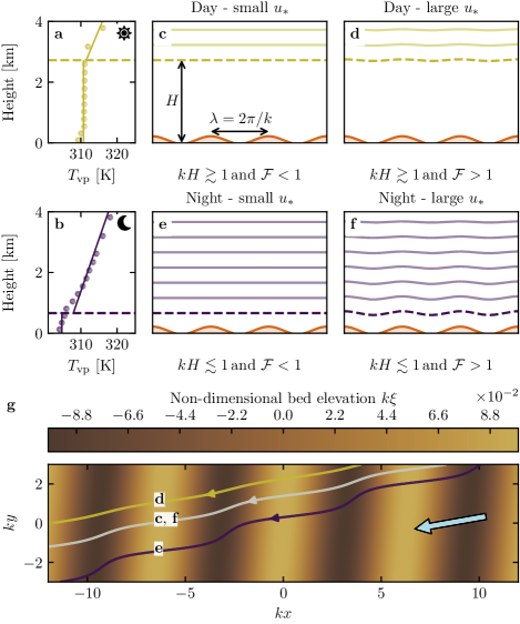
Figure 7: a,b: Vertical profiles of the virtual potential temperature $T_{\rm vp}$ at two different time steps (day - 03/11/2015 - 12.00 UTC, night - 01/13/2013 - 09.00 UTC) at the North Sand Sea station. Dots: data from the ERA5 reanalysis. Dashed lines: boundary layer height given by the ERA5 reanalysis (Online Resource section 2). Plain lines: vertical (boundary layer) and linear (free atmosphere) fits to estimate the stratification properties. c–f: Sketches representing the interaction between the giant dunes and the atmospheric flow for different meteorological conditions. g: Streamlines over a sinusoidal topography $\xi(x,y)$ qualitatively representing the effect of low, medium and strong flow confinement, in relation to the above panels (see Appendix Appendix 1: Linear Theory of Wind Response to Topographic Perturbation for more details). The blue arrow indicates the undisturbed wind direction.

3.1 Flow Over a Modulated Bed

Taking as a reference the turbulent flow over a flat bed, the general framework of our study is understanding and describing the flow response to a bed modulation (e.g. a giant dune). Without loss of generality, we can consider in this context an idealised bed elevation in the form of parallel sinusoidal ridges, with wavelength $\lambda$ (or wavenumber $k=2\pi/\lambda$) and amplitude $\xi_{0}$, and where the reference flow direction makes a given incident angle with respect to the ridge crest (Andreotti et al. 2012). Part of this response, on which we focus here, is the flow deflection by the ridges. In a simplified way, it can be understood from the Bernoulli principle (Hesp et al. 2015): as the flow approaches the ridge crest, the compression of the streamlines results in larger flow velocities, and thus lower pressures (Jackson and Hunt 1975). An incident flow oblique to the ridge is then deflected towards lower pressure zones, i.e towards the crest. Turbulent dissipation tends to increase this effect downstream, resulting in wind deflection along the crest in the lee side (Gadal et al. 2019).

Flow confinement below a capping surface, which enhances streamline compression, has a strong effect on the hydrodynamic response and typically increases flow deflection. This is the case for bedforms forming in open channel flows such as rivers (Kennedy 1963; Chang and Simons 1970; Mizumura 1995; Colombini 2004; Fourrière et al. 2010; Andreotti et al. 2012; Unsworth et al. 2018). This is also relevant for aeolian dunes as they evolve in the turbulent atmospheric boundary layer (ABL) capped by the stratified free atmosphere (FA) (Andreotti et al. 2009). Two main mechanisms, associated with dimensionless numbers must then be considered (Fig. 7). First, topographic obstacles typically disturb the flow over a characteristic height similar to their length. As flow confinement is characterised by a thickness $H$, the interaction between the dunes and the wind in the ABL is well captured by the parameter $kH$. The height $H$ is directly related to the sensitive heat flux from the Earth surface. It is typically on the order of a kilometre, but significantly varies with the circadian and seasonal cycles. Emerging and small dunes, with wavelengths in the range $20$ to $100$ m, are not affected by the flow confinement, corresponding to $kH\gg 1$. For giant dunes with kilometer-scale wavelengths, however, their interaction with the FA can be significant (Andreotti et al. 2009). This translates into a parameter $kH$ in the range $0.02$–$5$, depending on the moment of the day and the season. A second important mechanism is associated with the existence of a thin intermediate so-called capping layer between the ABL and the FA. It is characterised by a density jump $\Delta\rho$, which controls the ‘rigidity’ of this interface, i.e. how much its deformation affects streamline compression. This is usually quantified using the Froude number (Vosper 2004; Stull 2006; Sheridan and Vosper 2006; Hunt et al. 2006; Jiang 2014):

$$\mathcal{F}=\displaystyle\frac{U}{\sqrt{\displaystyle\frac{\Delta\rho}{\rho_{0}}gH}},$$ (1)

where $U$ is the wind velocity at the top of the ABL and $\rho_{0}$ its average density. The intensity of the stratification, i.e. the amplitude of the gradient $\left|\partial_{z}\rho\right|$ in the FA, also impacts the ability to deform the capping layer under the presence of an underlying obstacle, and thus affects the influence of flow confinement. This can be quantified using the internal Froude number (Vosper 2004; Stull 2006; Sheridan and Vosper 2006; Hunt et al. 2006; Jiang 2014) $\mathcal{F}_{\textup{I}}=kU/N$, where $N=\sqrt{-g\partial_{z}\rho/\rho_{0}}$ is the the Brunt-Väisälä frequency (Stull 1988). Both Froude numbers have in practice the same qualitative effect on flow confinement (a smaller Froude corresponding to a stiffer interface), and we shall restrict the main discussion to $\mathcal{F}$ only.

With this theoretical framework in mind, and in the context of the measured wind data in the North and South Sand Sea stations, the smallest wind disturbances are expected to occur during the day, when the ABL depth is the largest and comparable to the dune wavelength ($kH\gtrsim 1$), which corresponds to a weak confinement situation (Fig. 7c and d). In contrast, large wind disturbances are expected to occur during the night, when the confinement is mainly induced by a shallow ABL (Fig. 7e). However, this strong confinement can be somewhat reduced in the case of strong winds, corresponding to large values of the Froude number and a less ‘rigid’ interface (Fig. 7f). This is in qualitative agreement with the transition from deflected to non-deflected winds related to low and high velocities observed in our data (Sec. 2.2).

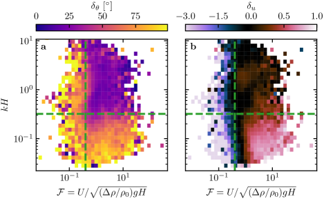
Figure 8: Regime diagrams of the wind deviation $\delta_{\theta}$ (a) and relative attenuation/amplification $\delta_{u}$ (b) in the space $(\mathcal{F},\,kH)$, containing the data from both the North Sand Sea and South Sand Sea stations. The green dashed lines empirically delimit the different regimes. The point density in each bin of the diagrams is shown in Online Resource Fig. S10 – 95% of the data occur in the range $-1<\delta u<1$. Similar regime diagrams in the spaces $(\mathcal{F}_{\textup{I}},\,kH)$ and $(\mathcal{F}_{\textup{I}},\,\mathcal{F})$ are shown in Online Resource Fig. S11.

3.2 Data Distribution in the Flow Regimes

We can go one step further and analyse how our data quantitatively spread over the different regimes discussed above. For that purpose, one needs to compute $kH$ and $\mathcal{F}$ from the time series. $H$, $U$ and the other atmospheric parameters can be deduced from the various vertical profiles (temperature, humidity) available in the ERA5 climate reanalysis (Online Resource section 2). We quantify the flow deflection $\delta_{\theta}$ as the minimal angle between the wind orientations comparing the local measurements and the regional predictions. We also compute the relative velocity modulation as

$$\delta_{\textup{u}}=\frac{u_{*}^{\textup{ERA5-Land}}-u_{*}^{\textup{Local mes.}}}{u_{*}^{\textup{ERA5-Land}}}.$$ (2)

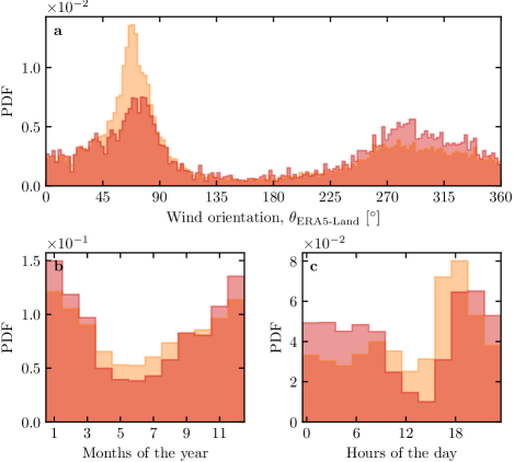
Figure S12: Normalized distributions of amplified velocities for the North sand Sea (light orange: $\delta_{u}<0$, orange: $\delta_{u}<-0.5$). a: Angular distributions. b: Monthly distributions. c: Hourly distributions.

These two quantities are represented as maps in the plane $(\mathcal{F},\,kH)$ (Fig. 8a and b), and one can clearly identify different regions in these plots. Small wind disturbances (small $\delta_{\theta}$ and $\delta_{\textup{u}}$) are located in the top-right part of the diagrams, corresponding to a regime with low-interaction as well as low-confinement ($kH$ and $\mathcal{F}$ large enough, Fig. 7d). Lower values of $kH$ (stronger interaction) or of Froude number (stronger confinement) both lead to an increase in wind disturbances, both in terms of orientation and velocity. Below a crossover value $kH\simeq 0.3$, wind disturbance is less sensitive to the $\mathcal{F}$-value. This is probably due to enhanced non-linear effects linked to flow modulation by the obstacle when confinement is strong (e.g. wakes and flow recirculations). The Froude number also controls a transition from damped to amplified wind velocities in the interdune, with a crossover around $\mathcal{F}\simeq 0.4$ (Fig. 8b). Such an amplification is rather unexpected. Checking the occurrence of the corresponding data, it appears that these amplifications are associated with the southerly sea breeze, and occur dominantly during the October-March period, when the other easterly wind is not present (Online Resource Fig. S12a–b). Furthermore, they occur less frequently during the afternoon, and more frequently at the end of the day (Online Resource Fig. S12c). This effect may be linked to a change in the flow behaviour in the lee side of the obstacles but further measurements are needed in order to assess the different possibilities (Baines 1995; Vosper 2004).

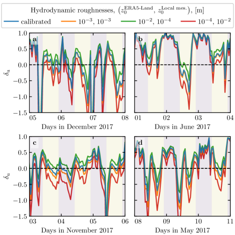
Figure S14: Time series of the relative velocity disturbance $\delta_{u}$ corresponding to Fig. 5, for different values of the hydrodynamic roughnesses. a: North Sand Sea – summer, b: North Sand Sea – winter, d: South Sand Sea – summer, e: South Sand Sea – winter. Note that $\delta_{\theta}$ is independent of the choice of $z_{0}^{\textup{ERA5-Land}}$ and $z_{0}^{\textup{Local mes.}}$.

As the hydrodynamic roughness $z_{0}$ determine the magnitude of wind shear velocities, Froude number $\mathcal{F}$ and relative velocity modulation $\delta_{u}$, it is important to discuss the sensitivity of the results to the $z_{0}$-values chosen for both the ERA5-Land and the field data (see Online Resource Sect. 1. Shear velocity and calibration of the hydrodynamical roughness). Other quantities associated with wind direction are independent of this choice. Considering the possible range of realistic roughness values, the uncertainty on velocities estimated using the law of the wall is at most 30 %. A similar maximum uncertainty applies to the Froude number. This uncertainty also propagates to $\delta_{u}$, for which Figure S14 shows that the choice of roughness has little influence on its temporal variations,even if it can induce a global increase or decrease of its values. Hence, the choice of the $z_{0}$-values will not qualitatively affect the overall aspect of the regime diagram presented in Figure 8b. It may only change the value of $\delta_{u}$ for which the transition between regimes is observed (dashed green lines in Figure 8b). Our conclusions are thus robust with respect to the somewhat arbitrary choice of the hydrodynamic roughness values.

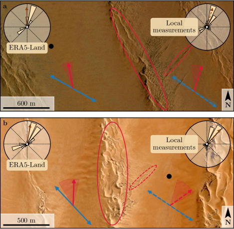
Figure 9: Implications for smaller scale patterns in (a) the South Sand Sea and (b) North Sand Sea. The ellipses indicate the different types of elongating dunes, at large (plain line) and small (dashed line) scales. Dune orientation are predicted using the model of Courrech du Pont et al. (2014) from the sand flux angular distributions, shown here (roses) along with the resultant transport direction (brown arrow) for typical values (grain size $180~{}\mu$m, flux-up ratio of $1.6$). Code for corresponding arrows: use of ERA5-Land data (plain line), use of local measurements (dashed line), prediction for the bed instability growth mechanism (blue), prediction for the elongation growth mechanism (red). Wedges show the uncertainty on the orientation calculation when parameters are varied. The black dots indicate the location of the meteorological stations in the interdune. See Appendix Appendix 2: Sediment Transport and Dune Morphodynamics for additional details.

4 Discussion and Conclusion

The feedback of the giant dunes on the wind flow has important implications for smaller scale bedforms. As illustrated in Fig. 9, small linear dunes ($\sim 50$ m wide) are often present within the 1–2 km interdune spaces between giant linear dunes in the Namib Sand Sea (Livingstone et al. 2010). These smaller dunes do not exhibit the same orientation as the large ones, and are sometimes named ‘crossing dunes’ (Chandler et al. 2022). Whilst differences between large and small scale dune patterns are observed ubiquitously, they are usually attributed to the presence of two different dune growth mechanisms, leading to two different dune patterns (orientations and/or morphologies) for the same wind regime (Courrech du Pont et al. 2014; Runyon et al. 2017; Lü et al. 2017; Song et al. 2019; Gadal et al. 2020; Hu et al. 2021). Here, however, our arguments enable the development of differing orientations for the small and giant linear dunes governed by the same dune growth mechanism (elongating mode). Figure 9 shows how the orientations for the small and giant dunes can be derived from the locally measured and regionally predicted winds respectively (red arrows in Fig. 9). These predictions require the threshold of aeolian sand transport to be specified. Importantly, its value (a shear velocity estimated at $u_{\textup{th}}\simeq 0.15~{}\textup{m}~{}\textup{s}^{-1}$ – see Appendix Appendix 2: Sediment Transport and Dune Morphodynamics) can be reached in periods during which deflected winds are observed (recall that the stronger winds, responsible for most of the sediment transport and associated dune morphodynamics, are not deflected – see Fig. 6). The feedback of the giant dunes on the wind described in this study, through wind deflection and attenuation, thus provides a potential explanation for the existence of these small linear dunes elongating across the interdune, a dynamic which has remained unresolved to date. These crossing dunes could provide additional constraints for the inference of local winds from bedforms, similarly to that currently performed on Mars using ripple orientations (Liu and Zimbelman 2015; Hood et al. 2021). Further work is needed to investigate these processes in more detail, including measurements of sediment transport and flow on the top of dunes.

This study presents field and reanalysis-based evidence that wind flow patterns around giant dunes are influenced by the atmospheric boundary layer, particularly during nocturnal conditions. However, we do not address here the question of the limitation of the giant dune pattern coarsening, and leave open the debate as to whether their size is controlled by the depth of this layer (Andreotti et al. 2009), in contrast to sediment supply limited and ever-slower growth with size (Werner and Kocurek 1999; Gunn et al. 2022). More field evidence is definitively needed from additional dune fields, but this mechanism would allow for the inference of the ABL depth from giant bedform wavelengths where measurements are not feasible or available, such as Titan (Lorenz et al. 2010).

To conclude on conditions under which the ERA5-Land reanalysis data can reliably be used to study dune morphodynamics, we summarise the comparison of local (direct measurements) and regional (climate reanalysis) wind data as follows. In flat areas, the agreement between the two confirms the ability of the ERA5-Land climate reanalysis to predict the wind regime down to scales $\sim 10$ km, i.e the model grid. When smaller scale topographies are present (giant dunes in our case), locally measured winds can significantly differ from the regionally predicted ones. This is the case when the disturbances induced by the dunes interact with the lower part of the ABL vertical structure, which presents circadian variations. During the day, when the capping layer is typically high, this interaction is small, and the ERA5-Land predictions are also quantitatively consistent with the local data. During the night, however, the presence of a shallow atmospheric boundary layer induces a strong confinement of the flow, and is associated with large wind deflection by the dunes. Importantly, we find that this effect can be counterbalanced for large wind velocities, which are capable of deforming the capping layer, thus decreasing the influence of the confinement.

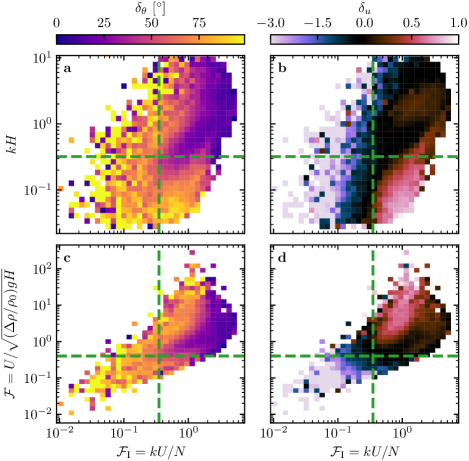
Figure S11: Regime diagrams of the wind deviation $\delta_{\theta}$ and relative attenuation/amplification $\delta_{u}$ in the spaces $(\mathcal{F}_{\textup{I}},\,kH)$ and $(\mathcal{F}_{\textup{I}},\,\mathcal{F})$, containing the data from both the North Sand Sea and South Sand Sea stations. Green dashed lines empirically delimit the different regimes. The point density in each bin of the diagrams is shown in Online Resource Fig. S10 – 95% of the data occur in the range $-1<\delta u<1$. The similar regime diagrams in the space $(\mathcal{F},\,kH)$ are shown in Fig. 8.

The theoretical computation of the wind disturbances induced by sinusoidal ridges under flow confinement has been performed in the linear limit (Andreotti et al. 2009, 2012), i.e. when the aspect ratio of these ridges is small ($k\xi_{0}\ll 1$). These models are able to qualitatively reproduce the observed wind deflection (Appendix Appendix 1: Linear Theory of Wind Response to Topographic Perturbation, Online Resource Figs. S11 and S13), and thus provide the physical support for the interpretation we propose here based on hydrodynamic regimes. However, these models cannot quantitatively predict the magnitude of our observations, probably due to the presence of expected non-linearities in high confinement situations linked to strong flow modulations. Besides, these linear calculations only predict wind attenuation in the interdune, in contrast with the observed enhanced velocities associated with particular evening winds from the south during the period October-March (Online Resource Fig. S12). Some other models predict different spatial flow structures in response to a modulated topography, such as lee waves and rotors (Baines 1995; Vosper 2004). However, our measurements are located at a single point in the interdune, and we are thus unable to explore these types of responses. Data at different places along and across the ridges are needed to investigate and possibly map such flow structures, and for further comparisons with the models.

Data Availability All data used in this study can be found in Gadal et al. (2022). Note that it contains modified Copernicus Climate Change Service Information (2021). Neither the European Commission nor ECMWF is responsible for any use that may be made of the Copernicus Information or Data it contains. Documented codes used in this study to analyse this data are available at https://github.com/Cgadal/GiantDunes (will be made public upon acceptance of this manuscript for publication).

Fundings Multiple grants have supported the collection of wind data through visits to the four sites between 2013 and 2020 (John Fell Oxford University Press (OUP) Research Fund (121/474); National Geographic (CP-029R-17); Natural Environment Research Council UK (NE/R010196/1 and NE/H021841/1 NSFGEO-NERC); Southampton Marine and Maritime Institute SMMI EPSRC-GCRF UK), along with research permits (1978/2014, 2140/2016, 2304/2017, 2308/2017, RPIV00022018, RPIV0052018, RPIV00230218). The authors are very grateful for support from Etosha National Park (especially Shyane Kötting, Boas Erckie, Pierre du Preez, Claudine Cloete, Immanuel Kapofi, Wilferd Versfeld, and Werner Kilian), Gobabeb Namib Research Institute (Gillian Maggs-Kölling and Eugene Marais), The Skeleton Coast National Park (Joshua Kazeurua). Various researchers and desert enthusiasts have assisted with instruments and the logistics of expeditions, especially Mary Seely for expert guidance at the North Sand Sea site. Finally, we acknowledge financial support from the Laboratoire d’Excellence UnivEarthS Grant ANR-10-LABX-0023, the Initiative d’Excellence Université de Paris Grant ANR-18-IDEX-0001, the French National Research Agency Grants ANR-17-CE01-0014/SONO and the National Science Center of Poland Grant 2016/23/B/ST10/01700.

Conflict of interest The authors declare that they have no conflict of interest.

Appendix 1: Linear Theory of Wind Response to Topographic Perturbation

Following the work of Fourrière et al. (2010), Andreotti et al. (2012) and Andreotti et al. (2009), we briefly describe in this appendix the framework for the linear response of a turbulent flow to a topographic perturbation of small aspect ratio. As a general bed elevation can be decomposed into Fourier modes, we focus here on a sinusoidal topography:

$$\xi=\xi_{0}\cos\left[k\left(\cos(\alpha)y-\sin(\alpha)x\right)\right],$$ (3)

which is also a good approximation for the giant dunes observed in the North Sand Sea and South Sand Sea Station (Fig. 2 and Online Resource Fig. S4). Here, $x$ and $y$ are the streamwise and spanwise coordinates, $k=2\pi/\lambda$ the wavenumber of the sinusoidal perturbation, $\alpha$ its crest orientation with respect to the $x$-direction (anticlockwise) and $\xi_{0}$ its amplitude. The two components of the basal shear stress $\boldsymbol{\tau}=\rho_{0}u_{*}\boldsymbol{u}_{*}$, constant in the flat bottom reference case, can then be generically written as:

$$\tau_{x} =\tau_{0}\left(1+k\xi_{0}\sqrt{\mathcal{A}_{x}^{2}+\mathcal{B}_{x}^{2}}\cos\left[k\left(\cos(\alpha)y-\sin(\alpha)x\right)+\phi_{x}\right]\right),$$ (4)

$$\tau_{y} =\tau_{0}\,k\xi_{0}\sqrt{\mathcal{A}_{y}^{2}+\mathcal{B}_{y}^{2}}\cos\left[k\left(\cos(\alpha)y-\sin(\alpha)x\right)+\phi_{y}\right],$$ (5)

where $\tau_{0}$ is the reference basal shear stress on a flat bed. We have defined the phase $\phi_{x,y}=\tan^{-1}\left(\mathcal{B}_{x,y}/\mathcal{A}_{x,y}\right)$ from the in-phase and in-quadrature hydrodynamical coefficients $\mathcal{A}_{x,y}$ and $\mathcal{B}_{x,y}$. They are functions of $k$ and of the flow conditions, i.e the bottom roughness, the vertical flow structure and the incident flow direction, and the theoretical framework developed in the above cited papers proposes methods to compute them in the linear regime.

Following Andreotti et al. (2012), the effect of the incident wind direction can be approximated by the following expressions:

$$\mathcal{A}_{x} =\mathcal{A}_{0}\sin^{2}\alpha,$$ (6)

$$\mathcal{B}_{x} =\mathcal{B}_{0}\sin^{2}\alpha,$$ (7)

$$\mathcal{A}_{y} =-\displaystyle\frac{1}{2}\mathcal{A}_{0}\cos\alpha\sin\alpha,$$ (8)

$$\mathcal{B}_{y} =-\displaystyle\frac{1}{2}\mathcal{B}_{0}\cos\alpha\sin\alpha,$$ (9)

where $\mathcal{A}_{0}$ and $\mathcal{B}_{0}$ are now two coefficients independent of the dune orientation $\alpha$, corresponding to the transverse case ($\alpha=90$). In the case of a fully turbulent boundary layer capped by a stratified atmosphere, these coefficients depend on $kH$, $kz_{0}$, $\mathcal{F}$ and $\mathcal{F}_{\textup{I}}$ (Andreotti et al. 2009). For their computation, we assume here a constant hydrodynamic roughness $z_{0}\simeq 1$ mm (Online Resource section 1). For the considered giant dunes, this leads to $kz_{0}\simeq 2\cdot 10^{-6}$, as their wavelength is $\lambda\simeq 2.4$ km (or $k\simeq 2\cdot 10^{-3}$ m^-1). Values of $z_{0}$ extracted from field data indeed typically fall between 0.1 mm and 10 mm (Sherman and Farrell 2008; Field and Pelletier 2018). Importantly, $\mathcal{A}_{0}$ and $\mathcal{B}_{0}$ do not vary much in the corresponding range of $kz_{0}$ (Fourrière et al. 2010), and the results presented here are robust with respect to this choice.

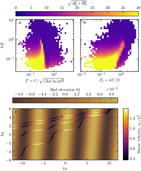
Figure S13: Computation of the flow disturbance with the linear model of Andreotti et al. (2009). a–b: Magnitude of the hydrodynamic coefficients $\mathcal{A}_{0}$ and $\mathcal{B}_{0}$, calculated from the time series of the non-dimensional numbers corresponding to the ERA5-Land wind data and ERA5 data on vertical pressure levels. c Shear velocity streamlines over sinusoidal ridges of amplitude $k\xi_{0}=0.1$ and for increasing values of $\sqrt{\mathcal{A}_{0}^{2}+\mathcal{B}_{0}^{2}}$. From the upper to the lower streamline, values of $\left(kH,\,\mathcal{F},\,\mathcal{F}_{\rm I},\,\mathcal{A}_{0},\,\mathcal{B}_{0},\,\sqrt{\mathcal{A}_{0}^{2}+\mathcal{B}_{0}^{2}}\right)$ are (1.9, 0.6, 1.5, 3.4, 1.0, 3.5), (1.5, 0.3, 0.4, 4.8, 1.4, 5.0), (0.1, 3.5, 1.0, 8.6, 0.1, 8.6), (0.5, 0.05, 0.04, 9.6, 2.5, 9.9).

With capping layer height and Froude numbers computed from the ERA5-Land time series, the corresponding $\mathcal{A}_{0}$ and $\mathcal{B}_{0}$ can be deduced, as displayed in Online Resource Fig. S13. Interestingly, it shows similar regimes as in the diagrams of Fig. 8 and Online Resource Fig. S11a,b, supporting the underlying physics. However, the agreement is qualitative only. Further, the linearity assumption of the theoretical framework requires $\left(|\tau|-\tau_{0}\right)/\tau_{0}\ll 1$, which translates into $k\xi\sqrt{\mathcal{A}_{0}^{2}+\mathcal{B}_{0}^{2}}\ll 1$. In our case, the giant dune morphology gives $k\xi_{0}\simeq 0.1$, which means that one quits the regime of validity of the linear theory when the coefficient modulus $\sqrt{\mathcal{A}_{0}^{2}+\mathcal{B}_{0}^{2}}$ becomes larger than a few units. In accordance with the theoretical expectations, these coefficients present values on the order of unity ($\mathcal{A}_{0}\simeq 3$ and $\mathcal{B}_{0}\simeq 1$) in unconfined situations (Claudin et al. 2013; Lü et al. 2021). In contrast and as illustrated in Online Resource Fig. S13a,b, larger values are predicted in case of strong confinement, which does not allow us to proceed to further quantitative comparison with the data.

Finally, the linear model is also able to reproduce the enhancement of the flow deflection over the sinusoidal ridges when $\sqrt{\mathcal{A}_{0}^{2}+\mathcal{B}_{0}^{2}}$ is increased (Online Resource Fig. S13). Here, using $k\xi_{0}\simeq 0.1$ to be representative of the amplitude of the giant dunes at the North Sand Sea station, the coefficient modulus is bounded to $10$.

Appendix 2: Sediment Transport and Dune Morphodynamics

We summarise in this appendix the sediment transport and dune morphodynamics theoretical framework leading to the prediction of sand fluxes and dune orientations from wind data.

Sediment Transport

— The prediction of sand fluxes from wind data has been a long standing issue in aeolian geomorphological studies (Fryberger and Dean 1979; Pearce and Walker 2005; Sherman and Li 2012; Shen et al. 2019). Based on laboratory studies in wind tunnels (Rasmussen et al. 1996; Iversen and Rasmussen 1999; Creyssels et al. 2009; Ho et al. 2011), as well as physical considerations (Ungar and Haff 1987; Andreotti 2004; Durán et al. 2011; Pähtz and Durán 2020), it has been shown that the steady saturated saltation flux over a flat sand bed depends linearly on the shear stress:

$$\frac{q_{\textup{sat}}}{Q}=\Omega\sqrt{\Theta_{\textup{th}}}\left(\Theta-\Theta_{\textup{th}}\right),$$ (10)

where $\Omega$ is a proportionality constant, $Q=d\sqrt{(\rho_{\textup{s}}-\rho_{0})gd/\rho_{0}}$ is a characteristic flux, $\Theta=\rho_{0}u_{*}^{2}/(\rho_{\textup{s}}-\rho_{0})gd$ the Shields number, and $\Theta_{\textup{th}}$ its threshold value below which saltation vanishes. $\rho_{\textup{s}}=2.6~{}\textup{g}~{}\textup{cm}^{-3}$ and $d=180~{}\mu\textup{m}$ are the grain density and diameter, and $g$ is the gravitational acceleration. The shear velocity, and consequently the Shields number as well as the sediment flux, are time dependent.

Recently, Pähtz and Durán (2020) suggested an additional quadratic term in Shields to account for grain-grain interactions within the transport layer at strong wind velocities:

$$\frac{q_{\textup{sat, t}}}{Q}=\frac{2\sqrt{\Theta_{\textup{th}}}}{\kappa\mu}\left(\Theta-\Theta_{\textup{th}}\right)\left(1+\frac{C_{\textup{M}}}{\mu}\left[\Theta-\Theta_{\textup{th}}\right]\right),$$ (11)

where $\kappa=0.4$ is the von Kármán constant, $C_{\rm M}\simeq 1.7$ a constant and $\mu\simeq 0.6$ is a friction coefficient, taken to be the avalanche slope of the granular material. The fit of this law to the experimental data of Creyssels et al. (2009) and Ho et al. (2011) gives $\Theta_{\textup{th}}=0.0035$. The fit of Eq. 10 on these same data similarly gives $\Omega\simeq 8$ and $\Theta_{\textup{th}}=0.005$. The sand flux angular distributions and the dune orientations in Fig. 9 are calculated using this law (11). We have checked that using the ordinary linear relationship (10) instead does not change the predicted dune orientations by more than a few degrees.

Dune Orientations

— Dune orientations are predicted with the dimensional model of Courrech du Pont et al. (2014), from the sand flux time series computed with the above transport law. Two orientations are possible depending on the mechanism dominating the dune growth: elongation or bed instability. The orientation $\alpha$ corresponding to the bed instability is then the one that maximises the following growth rate (Rubin and Hunter 1987):

$$\sigma\propto\frac{1}{H_{d}W_{d}T}\int_{0}^{T}q_{\textup{crest}}|\sin\left(\theta-\alpha\right)|\,\textup{d}t,$$ (12)

where $\theta$ is the wind orientation measured with respect to the same reference as $\alpha$, and $H_{d}$ and $W_{d}$ are dimensional constants respectively representing the dune height and width. The integral runs over a time $T$, which must be representative of the characteristic period of the wind regime. The flux at the crest is expressed as:

$$q_{\textup{crest}}=q_{\textup{sat}}\left[1+\gamma|\sin\left(\theta-\alpha\right)|\right],$$ (13)

where the flux-up ratio $\gamma$ has been calibrated to $1.6$ using field studies, underwater laboratory experiments and numerical simulations. Predictions of the linear analysis of Gadal et al. (2019) and Delorme et al. (2020) give similar results.

Similarly, the dune orientation corresponding to the elongation mechanism is the one that verifies:

$$\tan(\alpha)=\frac{\langle q_{\textup{crest}}(\alpha)\boldsymbol{e}_{\theta}\rangle\cdot\boldsymbol{e}_{WE}}{\langle q_{\textup{crest}}(\alpha)\boldsymbol{e}_{\theta}\rangle\cdot\boldsymbol{e}_{SN}},$$ (14)

where $\langle.\rangle$ denotes a vectorial time average. The unitary vectors $\boldsymbol{e}_{WE}$, $\boldsymbol{e}_{SN}$ and $\boldsymbol{e}_{\theta}$ are in the West-East, South-North and wind directions, respectively.

The resulting computed dune orientations, blue and red arrows in Fig. 9, then depend on a certain number of parameters (grain properties, flux-up ratio, etc.), for which we take typical values for aeolian sandy deserts. Due to the lack of measurements in the studied places, some uncertainties can be expected. We therefore run a sensitivity test by calculating the dune orientations for grain diameters ranging from $100~{}\mu\textup{m}$ to $400~{}\mu\textup{m}$ and for a speed-up ratio between $0.1$ and $10$ (wedges in Fig. 9).

C. Gadal^∗ $\cdot$ P. Delorme $\cdot$ C. Narteau $\cdot$ G.F.S. Wiggs $\cdot$ M. Baddock $\cdot$ J.M. Nield $\cdot$ P. Claudin

^∗ Institut de Mécanique des Fluides de Toulouse, Université de Toulouse Paul Sabatier, CNRS, Toulouse INP-ENSEEIHT, Toulouse, France.
cyril.gadal@imft.fr

1. Shear velocity and calibration of the hydrodynamical roughness

As the regionally predicted and locally measured velocities are available at different heights, we can not compare them directly. We therefore convert all velocities into shear velocities $u_{*}$, characteristic the turbulent logarithmic velocity profile (Spalding 1961; Stull 1988):

$$\frac{u(z)}{u_{*}}=\frac{1}{\kappa}\ln\left(\frac{z}{z_{0}}\right),$$ (15)

where $z$ is the vertical coordinate, $\kappa=0.4$ the von Kármán constant and $z_{0}$ the hydrodynamic roughness. Note that, strickly speaking, this logarithmic profile is valid for a neutrally stratified ABL only. Vertical density gradients occuring in other conditions may thus induce large discrepancies (Monin and Obukhov 1954; Garratt 1994; Dyer 1974). However, as our wind measurements are in the flow region close enough to the surface, where these effects are negligible, this logarithmic wind profile remains a farily good approximation in all conditions (Gunn et al. 2021). Several measurements of hydrodynamic roughnesses are available (Raupach 1992; Bauer et al. 1992; Brown et al. 2008; Nield et al. 2014). In the absence of sediment transport, it is governed by the geometric features of the bed (Flack and Schultz 2010; Pelletier and Field 2016). When aeolian saltation occurs, it is rather controlled by the altitude of Bagnold’s focal point (Durán et al. 2011; Valance et al. 2015), which depends on the wind velocity and grain properties (Sherman and Farrell 2008; Zhang et al. 2016; Field and Pelletier 2018). Whether associated with geometric features or with sediment transport, its typical order of magnitude is the millimetre scale on sandy surfaces.

We do not have precise velocity vertical profiles to be able to deduce an accurate value of $z_{0}$ in the various environments of the meteorological stations (vegetated, arid, sandy). Our approach is to rather select the hydrodynamic roughness which allows for the best possible matching between the regionally predicted and locally measured winds, i.e. minimising the relative difference $\delta$ between the wind vectors of both datasets:

$$\delta=\frac{\sqrt{\langle\|\boldsymbol{u}_{*,\textrm{era}}-\boldsymbol{u}_{*,\textrm{station}}\|^{2}\rangle}}{\sqrt{\langle\|\boldsymbol{u}_{*,\textrm{era}}\|\rangle\langle\|\boldsymbol{u}_{*,\textrm{station}}\|\rangle}},$$ (16)

where $\langle.\rangle$ denotes time average. This parameter is computed for values of $z_{0}$ in ERA5-Land analysis ranging from $10^{-5}$ m to $10^{-2}$ m for the four different stations. Note that for the North Sand Sea and South Sand Sea stations, where the giant dunes feedback presumably affect the wind, we take into account the non-deflected winds only in the calculation of $\delta$ (with a $15^{\circ}$ tolerance).

As shown in Online Resource Fig. S3, the minimum values of $\delta$ in the space ($z_{0}^{\textup{ERA5Land}}$, $z_{0}^{\textup{local}}$) form a line. We thus set the roughness in the ERA5-Land analysis to the typical value $z_{0}=10^{-3}$ m, and deduce the corresponding ones for the local stations. It leads to $2.7$, $0.8$, $0.1$ and $0.5$ mm for the Etosha West, North Sand Sea, Huab and South Sand Sea stations, respectively. Importantly, this approach somewhat impacts the calculation of the shear velocities, but not that of the wind directions. As such, most of our conclusions are independent of such a choice. However, it may affect the magnitude of the wind velocity attenuation/amplification in flow confinement situations.

2. Computation of the ABL characteristics

The estimation of the non-dimensional numbers associated with the ABL requires the computation of representative meteorological quantities. In arid areas, the vertical structure of the atmosphere can be approximated by a well mixed convective boundary layer of height $H$, topped by the stratified free atmosphere (Stull 1988; Shao 2008). In this context, one usually introduces the virtual potential temperature $T_{\textup{vp}}$, which is a constant $T_{0}$ inside the boundary layer, and increases linearly in the FA (Online Resource Fig. S8a):

$$T_{\textup{vp}}(z)=\begin{cases}T_{0}&\text{for $z\leq H$},\\ T_{0}\left(1+\displaystyle\frac{\Delta T_{\textup{vp}}}{T_{0}}+\frac{N^{2}}{g}(z-H)\right)&\text{for $z\geq H$},\end{cases}$$ (17)

where $\Delta T_{\textup{vp}}$ is the temperature discontinuity at the capping layer and $N=\sqrt{g\partial_{z}T_{\textup{vp}}/T_{0}}$ is the Brunt-Väisälä frequency, characteristic of the stratification. Note that, under the usual Boussinesq approximation, temperature and air density variations are simply related by $\delta T_{\textup{vp}}/T_{0}\simeq-\delta\rho/\rho_{0}$ (see Online Resource of Andreotti et al. (2009)), so that $N$ can equivalently be defined from the density gradient as next to (1).

The ERA5 dataset provides vertical profiles of the geopotential $\phi$, the actual temperature $T$ and the specific humidity $\eta$ at given pressure levels $P$. The vertical coordinate is then calculated as:

$$z=\frac{\phi R_{\textup{t}}}{gR_{\textup{t}}-\phi},$$ (18)

where $R_{\textup{t}}=6371229$ m is the reference Earth radius and $g=9.81$ m s^-2 is the gravitational acceleration. One also computes the virtual potential temperature as:

$$T_{\textup{vp}}=T\left[1+\left(\frac{M_{d}}{M_{w}}-1\right)\eta\right]\left(\frac{P_{0}}{P}\right)^{R/C_{p}},$$ (19)

where $P_{0}=10^{5}$ Pa is the standard pressure, $R=8.31$ J/K is the ideal gas constant, $C_{p}\simeq 29.1$ J/K is the air molar heat capacity, and $M_{w}=0.018$ kg/Mol and $M_{d}=0.029$ kg/Mol are the molecular masses of water and dry air respectively. The specific humidity is related to the vapour pressure $p_{w}$ as

$$\eta=\frac{\frac{M_{w}}{M_{d}}p_{w}}{p-\left(1-\frac{M_{w}}{M_{d}}\right)p_{w}}\,.$$ (20)

The ERA5 dataset also provides an estimate of the ABL depth $H$, based on the behaviour of the Richardson vertical profile. This dimensionless number is defined as the ratio of buoyancy and flow shear terms, and can be expressed as $\textup{Ri}=N^{2}/(\partial_{z}u)^{2}$. It vanishes in the lower well-mixed layer where $T_{\textup{vp}}$ is constant, and increases in the stratified FA. Following the method and calibration of Vogelezang and Holtslag (1996); Seidel et al. (2012), the value $\textup{Ri}(z)\simeq 0.25$ has been shown to be a good empirical criterion to give $z\simeq H$ within a precision varying from $50$% for the shallower ABL (e.g. at night) to $20$% for situations of stronger convection.

Examples of vertical virtual potential temperature profiles deduced from ERA5 are shown in Online Resource Fig. S8a. For each of them, an average temperature is computed below the ABL depth ($z<H$), and a linear function is fitted above, allowing us to extract the temperature jump $\Delta T_{\textup{vp}}$. Importantly, some profiles display a vertical structure that cannot be approximated by the simple form (17) used here (Online Resource Fig. S8b). In practice, we removed from the analysis all of those leading to the unphysical case $\Delta T_{\textup{vp}}<0$. We have noticed that these ‘ill-processed’ profiles dominantly occur in winter and are evenly spread across the hours of the day. Importantly, they represent $\simeq 12$% of the data only (Online Resource Fig. S8c,d), and we are thus confident that this data treatment does not affect our conclusions.

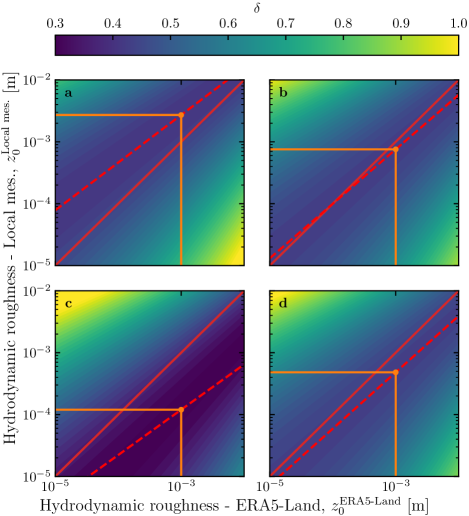
Figure S3: Calibration of hydrodynamic roughness. The parameter $\delta$ (16) quantifying the difference between local and predicted winds is shown in color scale as a function of the hydrodynamic roughnesses chosen for the ERA5-Land and for local winds, for the (a) Etosha West, (b) North Sand Sea, (c) Huab and (d) South Sand Sea stations. The red dashed and plain lines shows the minima of $\delta$ and the identity line, respectively. The orange lines and dots highlight the chosen hydrodynamic roughnesses for the local winds deduced from setting $z_{0}^{\textup{ERA5-Land}}=1$ mm.

Figure S7: Statistical comparison of the wind velocity between the ERA5-Land dataset and the local measurements for the South Sand Sea and North Sand Sea stations. a: Nocturnal summer easterly wind. b: Diurnal southerly wind. Black dashed lines are identity lines. The angle ranges used to select diurnal and nocturnal summer winds are the same as those in Figs. 4 and Figs. 6 of the main article.

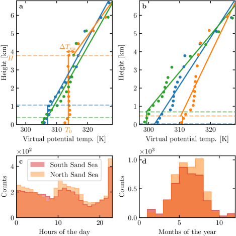
Figure S8: a: Vertical profiles of the virtual potential temperature at three different times (blue: 29/11/2012 - 11.00 UTC, orange: 21/03/2017 - 12.00 UTC, green: 21/03/2017 - 20.00 UTC) at the South Sand Sea station. Dots: data from the ERA5 reanalysis. Dashed lines: boundary layer height given by the ERA5 reanalysis. Plain lines: vertical (ABL) and linear (FA) fits to estimate the quantities displayed in Online Resource Fig. S9. b: Examples of ill-processed vertical profiles at three different times (blue: 2/12/2013 - 23.00 UTC, orange: 20/03/2017 - 00.00 UTC, green: 14/07/2017 - 14.00 UTC) at the South Sand Sea station. Distribution of ill-processed vertical profiles at South (orange) and North (light orange) Sand Sea station: hourly (c) and monthly (d) counts.

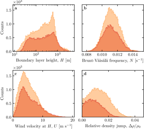
Figure S9: Distributions of the meteorological parameters resulting from the processing of the ERA5-Land data for the South Sand Sea (orange) and the North Sand Sea (light orange) stations.

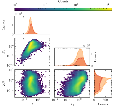
Figure S10: Non-dimensional parameters distributions. For the marginal distributions, the light orange corresponds to the South Sand Sea station, and the orange to the North Sand Sea station.

References

- Andreotti (2004) Andreotti B (2004) A two-species model of aeolian sand transport. J Fluid Mech 510:47–70
- Andreotti et al. (2002) Andreotti B, Claudin P, Douady S (2002) Selection of dune shapes and velocities part 1: dynamics of sand, wind and barchans. The European Physical Journal B-Condensed Matter and Complex Systems 28:321–339
- Andreotti et al. (2009) Andreotti B, Fourrière A, Ould-Kaddour F, Murray B, Claudin P (2009) Giant aeolian dune size determined by the average depth of the atmospheric boundary layer. Nature 457:1120–1123
- Andreotti et al. (2012) Andreotti B, Claudin P, Devauchelle O, Durán O, Fourrière A (2012) Bedforms in a turbulent stream: ripples, chevrons and antidunes. J Fluid Mech 690:94–128
- Ashkenazy et al. (2012) Ashkenazy Y, Yizhaq H, Tsoar H (2012) Sand dune mobility under climate change in the kalahari and australian deserts. Climatic Change 112:901–923
- Baddock et al. (2007) Baddock M, Livingstone I, Wiggs G (2007) The geomorphological significance of airflow patterns in transverse dune interdunes. Geomorphology 87:322–336
- Bagnold (1941) Bagnold RA (1941) The Physics of Blown Sand and Desert Dunes. London : Methuen : Chapman & Hall
- Baines (1995) Baines PG (1995) Topographic effects in stratified flows. Cambridge university press
- Bauer et al. (1992) Bauer BO, Sherman DJ, Wolcott JF (1992) Sources of uncertainty in shear stress and roughness length estimates derived from velocity profiles. The Professional Geographer 44:453–464
- Belcher and Hunt (1998) Belcher S, Hunt J (1998) Turbulent flow over hills and waves. Annu Rev Fluid Mech 30:507–538
- Blumberg and Greeley (1996) Blumberg DG, Greeley R (1996) A comparison of general circulation model predictions to sand drift and dune orientations. J Clim 9:3248–3259
- Bristow et al. (2022) Bristow NR, Best J, Wiggs GFS, Nield JM, Baddock MC, Delorme P, Christensen KT (2022) Topographic perturbation of turbulent boundary layers by low-angle, early-stage aeolian dunes. Earth Surf Process Landf n/a, DOI https://doi.org/10.1002/esp.5326
- Brookfield (1977) Brookfield M (1977) The origin of bounding surfaces in ancient aeolian sandstones. Sedimentology 24:303–332
- Brown et al. (2008) Brown S, Nickling WG, Gillies JA (2008) A wind tunnel examination of shear stress partitioning for an assortment of surface roughness distributions. J Geophys Res 113:F02S06
- Chandler et al. (2022) Chandler C, Radebaugh J, McBride J, Morris T, Narteau C, Arnold K, Lorenz R, Barnes J, Hayes A, Rodriguez S, Rittenour T (2022) Near-surface structure of a large linear dune and an associated crossing dune of the northern Namib Sand Sea from ground penetrating radar: Implications for the history of large linear dunes on Earth and Titan. Aeolian Research 57:100813, DOI https://doi.org/10.1016/j.aeolia.2022.100813
- Chang and Simons (1970) Chang H, Simons D (1970) The bed configuration of straight sand-bed channels when flow is nearly critical. J Fluid Mech 42:491–495
- Charru et al. (2013) Charru F, Andreotti B, Claudin P (2013) Sand ripples and dunes. Annu Rev Fluid Mech 45:469–493
- Claudin et al. (2013) Claudin P, Wiggs G, Andreotti B (2013) Field evidence for the upwind velocity shift at the crest of low dunes. Boundary-Layer Meteorol 148:195–206
- Claudin et al. (2017) Claudin P, Durán O, Andreotti B (2017) Dissolution instability and roughening transition. J Fluid Mech 832:R2
- Claudin et al. (2021) Claudin P, Louge M, Andreotti B (2021) Basal pressure variations induced by a turbulent flow over a wavy surface. Frontiers in Physics 9:682564
- Colombini (2004) Colombini M (2004) Revisiting the linear theory of sand dune formation. J Fluid Mech 502:1–16
- Courrech du Pont (2015) Courrech du Pont S (2015) Dune morphodynamics. C R Phys 16:118–138
- Courrech du Pont et al. (2014) Courrech du Pont S, Narteau C, Gao X (2014) Two modes for dune orientation. Geology 42:743–746
- Creyssels et al. (2009) Creyssels M, Dupont P, El Moctar AO, Valance A, Cantat I, Jenkins JT, Pasini JM, Rasmussen KR (2009) Saltating particles in a turbulent boundary layer: experiment and theory. J Fluid Mech 625:47–74
- de Winter et al. (2020) de Winter W, Donker J, Sterk G, Van Beem J, Ruessink G (2020) Regional versus local wind speed and direction at a narrow beach with a high and steep foredune. Plos one 15:e0226983
- Dee et al. (2011) Dee DP, Uppala SM, Simmons AJ, Berrisford P, Poli P, Kobayashi S, Andrae U, Balmaseda M, Balsamo G, Bauer dP, et al. (2011) The ERA-Interim reanalysis: Configuration and performance of the data assimilation system. Q J R Meteorol Soc 137:553–597
- Delorme et al. (2020) Delorme P, Wiggs G, Baddock M, Claudin P, Nield J, Valdez A (2020) Dune initiation in a bimodal wind regime. J Geophys Res 125:e2020JF005757
- Durán et al. (2011) Durán O, Claudin P, Andreotti B (2011) On aeolian transport: Grain-scale interactions, dynamical mechanisms and scaling laws. Aeolian Res 3:243–270
- Durran (1990) Durran DR (1990) Mountain waves and downslope winds. In: Atmospheric processes over complex terrain, Springer, pp 59–81
- Dyer (1974) Dyer A (1974) A review of flux-profile relationships. Boundary-Layer Meteorol 7:363–372
- Ewing et al. (2006) Ewing RC, Kocurek G, Lake LW (2006) Pattern analysis of dune-field parameters. Earth Surf Process Landf 31:1176–1191
- Farr et al. (2007) Farr TG, Rosen PA, Caro E, Crippen R, Duren R, Hensley S, Kobrick M, Paller M, Rodriguez E, Roth L, et al. (2007) The shuttle radar topography mission. Rev Geophys 45
- Fernando et al. (2019) Fernando H, Mann J, Palma J, Lundquist JK, Barthelmie RJ, Belo-Pereira M, Brown W, Chow F, Gerz T, Hocut C, et al. (2019) The perdigão: Peering into microscale details of mountain winds. Bull Am Meteorol Soc 100:799–819
- Field and Pelletier (2018) Field JP, Pelletier JD (2018) Controls on the aerodynamic roughness length and the grain-size dependence of aeolian sediment transport. Earth Surf Process Landf 43:2616–2626
- Finnigan et al. (1990) Finnigan J, Raupach M, Bradley E, Aldis G (1990) A wind tunnel study of turbulent flow over a two-dimensional ridge. Boundary-Layer Meteorol 50:277–317
- Finnigan et al. (2020) Finnigan J, Ayotte K, Harman I, Katul G, Oldroy H, Patton E, Poggi D, Ross A, Taylor P (2020) Boundary-layer flow over complex topography. Boundary-Layer Meteorol 177:247–313
- Flack and Schultz (2010) Flack K, Schultz M (2010) Review of hydraulic roughness scales in the fully rough regime. Journal of Fluids Engineering 132:041203
- Fourrière et al. (2010) Fourrière A, Claudin P, Andreotti B (2010) Bedforms in a turbulent stream: formation of ripples by primary linear instability and of dunes by nonlinear pattern coarsening. J Fluid Mech 649:287–328
- Frederick and Hanratty (1988) Frederick KA, Hanratty TJ (1988) Velocity measurements for a turbulent nonseparated flow over solid waves. Exp Fluids 6:477–486
- Fryberger and Dean (1979) Fryberger SG, Dean G (1979) Dune forms and wind regime. A study of global sand seas 1052:137–169
- Gadal et al. (2019) Gadal C, Narteau C, Courrech Du Pont S, Rozier O, Claudin P (2019) Incipient bedforms in a bidirectional wind regime. J Fluid Mech 862:490–516
- Gadal et al. (2020) Gadal C, Narteau C, Courrech du Pont S, Rozier O, Claudin P (2020) Periodicity in fields of elongating dunes. Geology 48:343–347
- Gadal et al. (2022) Gadal C, Delorme P, Narteau C, Wiggs G, Baddock M, Nield JM, Claudin P (2022) Data used in ’Local wind regime induced by giant linear dunes: comparison of ERA5-Land re-analysis with surface measurements’. DOI 10.5281/zenodo.6343138
- Gao et al. (2021) Gao X, Narteau C, Gadal C (2021) Migration of reversing dunes against the sand flow path as a singular expression of the speed-up effect. Journal of Geophysical Research: Earth Surface 126(5):e2020JF005913
- Garratt (1994) Garratt JR (1994) The atmospheric boundary layer. Earth-Science Reviews 37:89–134
- Garvey et al. (2005) Garvey B, Castro IP, Wiggs G, Bullard J (2005) Measurements of flows over isolated valleys. Boundary-Layer Meteorol 117:417–446
- Gong and Ibbetson (1989) Gong W, Ibbetson A (1989) A wind tunnel study of turbulent flow over model hills. Boundary-Layer Meteorol 49:113–148
- Gong et al. (1996) Gong W, Taylor P, Dörnbrack A (1996) Turbulent boundary-layer flow over fixed aerodynamically rough two-dimensional sinusoidal waves. J Fluid Mech 312:1–37
- Guérin et al. (2020) Guérin A, Derr J, Du Pont SC, Berhanu M (2020) Streamwise dissolution patterns created by a flowing water film. Phys Rev Lett 125:194502
- Gunn et al. (2021) Gunn A, Wanker M, Lancaster N, Edmonds D, Ewing R, Jerolmack D (2021) Circadian rhythm of dune-field activity. Geophys Res Lett 48:e2020GL090924
- Gunn et al. (2022) Gunn A, Casasanta G, Di Liberto L, Falcini F, Lancaster N, Jerolmack DJ (2022) What sets aeolian dune height? Nature communications 13(1):1–8
- Harris et al. (2020) Harris CR, Millman KJ, van der Walt SJ, Gommers R, Virtanen P, Cournapeau D, Wieser E, Taylor J, Berg S, Smith NJ, et al. (2020) Array programming with numpy. Nature 585:357–362
- Havholm and Kocurek (1988) Havholm KG, Kocurek G (1988) A preliminary study of the dynamics of a modern draa, Algodones, southeastern California, USA. Sedimentology 35:649–669
- Hersbach et al. (2020) Hersbach H, Bell B, Berrisford P, Hirahara S, Horányi A, Muñoz-Sabater J, Nicolas J, Peubey C, Radu R, Schepers D, et al. (2020) The ERA5 global reanalysis. Q J R Meteorol Soc 146:1999–2049
- Hesp et al. (1989) Hesp P, Illenberger W, Rust I, McLachlan A, Hyde R (1989) Some aspects of transgressive dunefield and transverse dune geomorphology and dynamics, south coast, South Africa. Zeitschrift fur Geomorphologie, Supplementband 73:111–123
- Hesp and Hastings (1998) Hesp PA, Hastings K (1998) Width, height and slope relationships and aerodynamic maintenance of barchans. Geomorphology 22:193–204
- Hesp et al. (2015) Hesp PA, Smyth TAG, Nielsen P, Walker IJ, Bauer BO, Davidson-Arnott R (2015) Flow deflection over a foredune. Geomorphology 230:64–74
- Ho et al. (2011) Ho TD, Valance A, Dupont P, Ould El Moctar A (2011) Scaling laws in aeolian sand transport. Phys Rev Lett 106:4–7
- Hood et al. (2021) Hood DR, Ewing RC, Roback KP, Runyon K, Avouac JP, McEnroe M (2021) Inferring airflow across martian dunes from ripple patterns and dynamics. Frontiers in Earth Science 9:702828
- Howard (1977) Howard AD (1977) Effect of slope on the threshold of motion and its application to orientation of wind ripples. Geological Society of America Bulletin 88:853–856
- Hu et al. (2021) Hu Z, Gao X, Lei J, Zhou N (2021) Geomorphology of aeolian dunes in the western Sahara Desert. Geomorphology 392:107916
- Hunt et al. (1988) Hunt J, Leibovich S, Richards K (1988) Turbulent shear flows over low hills. Q J R Meteorol Soc 114:1435–1470
- Hunt et al. (2006) Hunt JCR, Vilenski GG, Johnson ER (2006) Stratified separated flow around a mountain with an inversion layer below the mountain top. J Fluid Mech 556:105–119
- Hunter (2007) Hunter JD (2007) Matplotlib: A 2d graphics environment. Computing in science & engineering 9:90–95
- Hunter et al. (1983) Hunter RE, Richmond BM, Alpha TR (1983) Storm-controlled oblique dunes of the Oregon coast. Geol Soc America Bull 94:1450–1465
- Iversen and Rasmussen (1999) Iversen JD, Rasmussen KR (1999) The effect of wind speed and bed slope on sand transport. Sedimentology 46:723–731
- Jackson and Hunt (1975) Jackson PS, Hunt JCR (1975) Turbulent wind flow over a low hill. Q J R Meteorol Soc 101:929–955
- Jiang (2014) Jiang Q (2014) Applicability of reduced-gravity shallow-water theory to atmospheric flow over topography. J Atmos Sci 71:1460–1479
- Jolivet et al. (2021) Jolivet M, Braucher R, Dovchintseren D, Hocquet S, Schmitt J, ASTER Team (2021) Erosion around a large-scale topographic high in a semi-arid sedimentary basin: Interactions between fluvial erosion, aeolian erosion and aeolian transport. Geomorphology 386:107747
- Kennedy (1963) Kennedy JF (1963) The mechanics of dunes and antidunes in erodible-bed channels. J Fluid Mech 16:521–544
- Kim et al. (2000) Kim HG, Patel VC, Lee CM (2000) Numerical simulation of wind flow over hilly terrain. J Wind Eng Ind Aerodyn 87:45–60
- Kroy et al. (2002) Kroy K, Sauermann G, Herrmann HJ (2002) Minimal model for aeolian sand dunes. Phys Rev E 66:031302
- Lancaster et al. (1984) Lancaster J, Lancaster N, Seely M (1984) Climate of the central Namib desert. Madoqua 1984:5–61
- Lancaster (1985) Lancaster N (1985) Winds and sand movements in the Namib sand sea. Earth Surf Process Landf 10:607–619
- Lancaster et al. (1996) Lancaster N, Nickling W, Neuman CM, Wyatt V (1996) Sediment flux and airflow on the stoss slope of a barchan dune. Geomorphology 17:55–62
- Lewis et al. (2008) Lewis HW, Mobbs SD, Lehning M (2008) Observations of cross-ridge flows across steep terrain. Q J R Meteorol Soc 134:801–816
- Liu and Zimbelman (2015) Liu ZYC, Zimbelman JR (2015) Recent near-surface wind directions inferred from mapping sand ripples on martian dunes. Icarus 261:169–181
- Livingstone and Warren (2019) Livingstone I, Warren A (2019) Aeolian geomorphology: a new introduction. Wiley
- Livingstone et al. (2010) Livingstone I, Bristow C, Bryant RG, Bullard J, White K, Wiggs GFS, Baas ACW, Bateman MD, Thomas DSG (2010) The Namib Sand Sea digital database of aeolian dunes and key forcing variables. Aeolian Res 2:93–104
- Lorenz et al. (2010) Lorenz R, Claudin P, Andreotti B, Radebaugh J, Tokano T (2010) A 3 km atmospheric boundary layer on Titan indicated by dune spacing and Huygens data. Icarus 205:719–721
- Lü et al. (2017) Lü P, Narteau C, Dong Z, Rozier O, Du Pont SC (2017) Unravelling raked linear dunes to explain the coexistence of bedforms in complex dunefields. Nature Communications 8:1–9
- Lü et al. (2021) Lü P, Narteau C, Dong Z, Claudin P, Rodriguez S, An Z, Fernandez-Cascales L, Gadal C, Courrech du Pont S (2021) Direct validation of dune instability theory. Proceedings of the National Academy of Sciences 118
- Mason and Sykes (1979) Mason P, Sykes R (1979) Flow over an isolated hill of moderate slope. Q J R Meteorol Soc 105:383–395
- McKenna Neuman et al. (1997) McKenna Neuman C, Lancaster N, Nickling WG (1997) Relations between dune morphology, air flow, and sediment flux on reversing dunes, Silver Peak, Nevada. Sedimentology 44:1103–1111, DOI 10.1046/j.1365-3091.1997.d01-61.x
- Mizumura (1995) Mizumura K (1995) Free-surface profile of open-channel flow with wavy boundary. J Hydraul Eng 121:533–539
- Monin and Obukhov (1954) Monin AS, Obukhov AM (1954) Basic laws of turbulent mixing in the surface layer of the atmosphere. Contrib Geophys Inst Acad Sci USSR 151:e187
- Mulligan (1988) Mulligan KR (1988) Velocity profiles measured on the windward slope of a transverse dune. Earth Surf Process Landf 13:573–582
- Muñoz-Sabater et al. (2021) Muñoz-Sabater J, Dutra E, Agustí-Panareda A, Albergel C, Arduini G, Balsamo G, Boussetta S, Choulga M, Harrigan S, Hersbach H, et al. (2021) ERA5-Land: A state-of-the-art global reanalysis dataset for land applications. Earth Syst Sci Data 13:4349–4383
- Nield et al. (2014) Nield JM, King J, Wiggs GFS, Leyland J, Bryant RG, Chiverrell RC, Darby SE, Eckhardt FD, Thomas DSG, Vircavs LH, Washington R (2014) Estimating aerodynamic roughness over complex surface terrain. J Geophys Res 118:12948–12961
- Nield et al. (2017) Nield JM, Wiggs GG, Baddock MC, Hipondoka MH (2017) Coupling leeside grainfall to avalanche characteristics in aeolian dune dynamics. Geology 45:271–274
- Pähtz and Durán (2020) Pähtz T, Durán O (2020) Unification of aeolian and fluvial sediment transport rate from granular physics. Phys Rev Lett 124:168001
- Pearce and Walker (2005) Pearce KI, Walker IJ (2005) Frequency and magnitude biases in the ’Fryberger’ model, with implications for characterizing geomorphically effective winds. Geomorphology 68:39–55
- Pelletier and Field (2016) Pelletier JD, Field JP (2016) Predicting the roughness length of turbulent flows over landscapes with multi-scale microtopography. Earth Surface Dynamics 4:391–405
- Poggi et al. (2007) Poggi D, Katul G, Albertson J, Ridolfi L (2007) An experimental investigation of turbulent flows over a hilly surface. Phys Fluids 19:036601
- Rasmussen (1989) Rasmussen KR (1989) Some aspects of flow over coastal dunes. Proceedings of the Royal Society of Edinburgh, Section B: Biological Sciences 96:129–147
- Rasmussen et al. (1996) Rasmussen KR, Iversen JD, Rautaheimo P (1996) Saltation and wind flow interaction in a variable slope wind tunnel. Geomorphology 17:19–28
- Raupach (1992) Raupach M (1992) Drag and drag partition on rough surfaces. Boundary-Layer Meteorol 60:375–395
- Rozier et al. (2019) Rozier O, Narteau C, Gadal C, Claudin P, Courrech du Pont S (2019) Elongation and stability of a linear dune. Geophysical Research Letters 46(24):14521–14530
- Rubin and Hunter (1987) Rubin DM, Hunter RE (1987) Bedform alignment in directionally varying flows. Science 237:276–278
- Runyon et al. (2017) Runyon K, Bridges N, Ayoub F, Newman C, Quade J (2017) An integrated model for dune morphology and sand fluxes on Mars. Earth and Planetary Science Letters 457:204–212
- Sauermann et al. (2003) Sauermann G, Andrade Jr J, Maia L, Costa U, Araújo A, Herrmann H (2003) Wind velocity and sand transport on a barchan dune. Geomorphology 54:245–255
- Seidel et al. (2012) Seidel DJ, Zhang Y, Beljaars A, Golaz JC, Jacobson AR, Medeiros B (2012) Climatology of the planetary boundary layer over the continental United States and Europe. J Geophys Res 117:D17106
- Shao (2008) Shao Y (2008) Physics and modelling of wind erosion, vol 37. Springer Science & Business Media
- Shen et al. (2019) Shen Y, Zhang C, Huang X, Wang X, Cen S (2019) The effect of wind speed averaging time on sand transport estimates. Catena 175:286–293
- Sheridan and Vosper (2006) Sheridan PF, Vosper SB (2006) A flow regime diagram for forecasting lee waves, rotors and downslope winds. Meteorol Appl 13:179–195
- Sherman (1978) Sherman CA (1978) A mass-consistent model for wind fields over complex terrain. J Appl Meteorol Clim 17:312–319
- Sherman and Farrell (2008) Sherman D, Farrell E (2008) Aerodynamic roughness lengths over movable beds: Comparison of wind tunnel and field data. J Geophys Res 113:1–10
- Sherman and Li (2012) Sherman DJ, Li B (2012) Predicting aeolian sand transport rates: A reevaluation of models. Aeolian Res 3:371–378
- Smith et al. (2017) Smith AB, Jackson DWT, Cooper JAG (2017) Three-dimensional airflow and sediment transport patterns over barchan dunes. Geomorphology 278:28–42
- Song et al. (2019) Song Q, Gao X, Lei J, Li S (2019) Spatial distribution of sand dunes and their relationship with fluvial systems on the southern margin of the Taklimakan Desert, China. Geomatics, Natural Hazards and Risk 10:2408–2428
- Spalding (1961) Spalding DB (1961) A single formula for the law of the wall. Journal of Applied Mechanics 28:455–458
- Stull (2006) Stull R (2006) 9 - the atmospheric boundary layer. In: Wallace JM, Hobbs PV (eds) Atmospheric Science (Second Edition), second edition edn, Academic Press, San Diego, pp 375–417
- Stull (1988) Stull RB (1988) An introduction to boundary layer meteorology, vol 13. Springer Science & Business Media
- Sullivan and McWilliams (2010) Sullivan PP, McWilliams JC (2010) Dynamics of winds and currents coupled to surface waves. Annu Rev Fluid Mech 42:19–42
- Sweet and Kocurek (1990) Sweet M, Kocurek G (1990) An empirical model of aeolian dune lee-face airflow. Sedimentology 37:1023–1038
- Sykes (1980) Sykes RI (1980) An asymptotic theory of incompressible turbulent boundarylayer flow over a small hump. J Fluid Mech 101:647–670
- Taylor and Teunissen (1987) Taylor P, Teunissen H (1987) The Askervein hill project: overview and background data. Boundary-Layer Meteorol 39:15–39
- Taylor et al. (1987) Taylor P, Mason P, Bradley E (1987) Boundary-layer flow over low hills. Boundary-Layer Meteorol 39:107–132
- Tsoar and Yaalon (1983) Tsoar H, Yaalon DH (1983) Deflection of sand movement on a sinuous longitudinal (seif) dune: use of fluorescent dye as tracer. Sedimentary Geology 36:25–39
- Ungar and Haff (1987) Ungar JE, Haff PK (1987) Steady state saltation in air. Sedimentology 34:289–299
- Unsworth et al. (2018) Unsworth C, Parsons D, Hardy R, Reesink A, Best J, Ashworth P, Keevil G (2018) The impact of nonequilibrium flow on the structure of turbulence over river dunes. Water Resour Res 54:6566–6584
- Uppala et al. (2005) Uppala SM, Kållberg P, Simmons AJ, Andrae U, Bechtold VDC, Fiorino M, Gibson J, Haseler J, Hernandez A, Kelly G, et al. (2005) The ERA-40 re-analysis. Q J R Meteorol Soc 131:2961–3012
- Valance et al. (2015) Valance A, Rasmussen K, Ould El Moctar A, Dupont P (2015) The physics of aeolian sand transport. C R Phys 16:1–13
- Venditti et al. (2013) Venditti JG, Best JL, Church M, Hardy RJ (2013) Coherent Flow Structures at Earth’s Surface. John Wiley & Sons
- Virtanen et al. (2020) Virtanen P, Gommers R, Oliphant TE, Haberland M, Reddy T, Cournapeau D, Burovski E, Peterson P, Weckesser W, Bright J, et al. (2020) Scipy 1.0: fundamental algorithms for scientific computing in python. Nature methods 17:261–272
- Vogelezang and Holtslag (1996) Vogelezang D, Holtslag A (1996) Evaluation and model impacts of alternative boundary-layer height formulations. Boundary-Layer Meteorol 81:245–269
- Vosper (2004) Vosper SB (2004) Inversion effects on mountain lee waves. Q J R Meteorol Soc 130:1723–1748
- Walker et al. (2017) Walker I, Davidson-Arnott R, Bauer B, Hesp P, Delgado-Fernandez I, Ollerhead J, Smyth T (2017) Scale-dependent perspectives on the geomorphology and evolution of beach-dune systems. Earth-Science Review 171:220–253
- Walker and Nickling (2002) Walker IJ, Nickling WG (2002) Dynamics of secondary airflow and sediment transport over and in the lee of transverse dunes. Prog Phys Geogr 26:47–75
- Walker et al. (2006) Walker IJ, Hesp PA, Davidson-Arnott RG, Ollerhead J (2006) Topographic steering of alongshore airflow over a vegetated foredune: Greenwich Dunes, Prince Edward Island, Canada. Journal of Coastal Research 22:1278–1291
- Walker et al. (2009) Walker IJ, Hesp PA, Davidson-Arnott RG, Bauer BO, Namikas SL, Ollerhead J (2009) Responses of three-dimensional flow to variations in the angle of incident wind and profile form of dunes: Greenwich Dunes, Prince Edward Island, Canada. Geomorphology 105:127–138
- Walmsley et al. (1982) Walmsley JL, Salmon J, Taylor P (1982) On the application of a model of boundary-layer flow over low hills to real terrain. Boundary-Layer Meteorol 23:17–46
- Weaver and Wiggs (2011) Weaver C, Wiggs G (2011) Field measurements of mean and turbulent airflow over a barchan sand dune. Geomorphology 128:32–41
- Werner and Kocurek (1999) Werner BT, Kocurek G (1999) Bedform spacing from defect dynamics. Geology 27:727–730
- Wiggs et al. (2002) Wiggs G, Bullard J, Garvey B, Castro I (2002) Interactions between airflow and valley topography with implications for aeolian sediment transport. Physical Geography 23:366–380
- Wood (2000) Wood N (2000) Wind flow over complex terrain: a historical perspective and the prospect for large-eddy modelling. Boundary-Layer Meteorol 96:11–32
- Zhang et al. (2016) Zhang C, Li Q, Zhou N, Zhang J, Kang L, Shen Y, Jia W (2016) Field observations of wind profiles and sand fluxes above the windward slope of a sand dune before and after the establishment of semi-buried straw checkerboard barriers. Aeolian Res 20:59–70
- Zhang et al. (2014) Zhang D, Yang X, Rozier O, Narteau C (2014) Mean sediment residence time in barchan dunes. Journal of Geophysical Research: Earth Surface 119(3):451–463
- Zilker and Hanratty (1979) Zilker DP, Hanratty TJ (1979) Influence of the amplitude of a solid wavy wall on a turbulent flow. part 2. separated flows. J Fluid Mech 90:257–271
- Zilker et al. (1977) Zilker DP, Cook GW, Hanratty TJ (1977) Influence of the amplitude of a solid wavy wall on a turbulent flow. part 1. non-separated flows. J Fluid Mech 82:29–51
Local wind regime induced by giant linear dunes
— Supplementary Material —