Unsupervised Representation Learning in Deep Reinforcement Learning: A Review

Abstract

This review addresses the problem of learning abstract representations of the measurement data in the context of Deep Reinforcement Learning (DRL). While the data are often ambiguous, high-dimensional, and complex to interpret, many dynamical systems can be effectively described by a low-dimensional set of state variables. Discovering these state variables from the data is a crucial aspect for improving the data efficiency, robustness and generalization of DRL methods, tackling the curse of dimensionality, and bringing interpretability and insights into black-box DRL. This review provides a comprehensive and complete overview of unsupervised representation learning in DRL by describing the main Deep Learning tools used for learning representations of the world, providing a systematic view of the method and principles, summarizing applications, benchmarks and evaluation strategies, and discussing open challenges and future directions.

Keywords Reinforcement Learning  $\cdot$ Unsupervised Representation Learning  $\cdot$ Dynamical Systems

1 Introduction

Dynamical systems pervade our daily life. A pendulum swinging, a robot picking up objects, the flow of water in a river, the trend of economic costs, the spread of a disease and the prediction of climate change are all examples of dynamical systems. Understanding how these systems evolve by discovering the governing equations, how they react to inputs and how they can be controlled are crucial aspects of science, and engineering [1].

Governing equations are traditionally derived from physical principles, such as energy conservation laws and symmetries. However, many complex real-world dynamical systems exhibit strongly non-linear behaviours, making the discovery of the governing principles describing the evolution of the systems extremely challenging. Additionally, in many domains such as physical systems, robotics, economics, or health, we are interested not only into discovering the governing principles but also into controlling the dynamical systems via additional sets of input variables, called interchangeably control variables or actions, such that the systems manifest the desired behaviours. When turning to control, understanding how the systems react to changes of the control variables is crucial for obtaining optimal control laws.

In the last decade, Artificial Intelligence [2], Machine Learning (ML) [3] and data-driven methods have paved the road for new approaches to studying, analyzing, understanding and controlling dynamical systems. While data, in the forms of measurements of the systems, are often abundant, physical laws or governing equations are not always available. Even when present, they cannot fully capture the actual governing laws due to unknowns and uncertainties [4]. Traditional control techniques based on accurate models of the world are often unsuitable for such dynamical systems, making data-driven control methods, such as Reinforcement Learning (RL) [5], even more appealing.

RL is the branch of ML studying a computation approach for learning optimal behaviours – control laws – from interacting with the world to achieve predefined goals. RL founds its success in the Markov Decision Processes (MDPs) theory [6], and on the Nature-inspired paradigm of an intelligent agent , learning to act by interacting with an unknown environment and improving its behaviour based on the consequences of the actions taken. Consequences of the actions are quantified by a scalar signal called reward. RL faces the so-called curse of dimensionality [5] derived by continuous state and action spaces and by the high-dimensionality of the observable variables. The curse of dimensionality is common to many dynamical systems, making RL algorithms computationally inefficient.

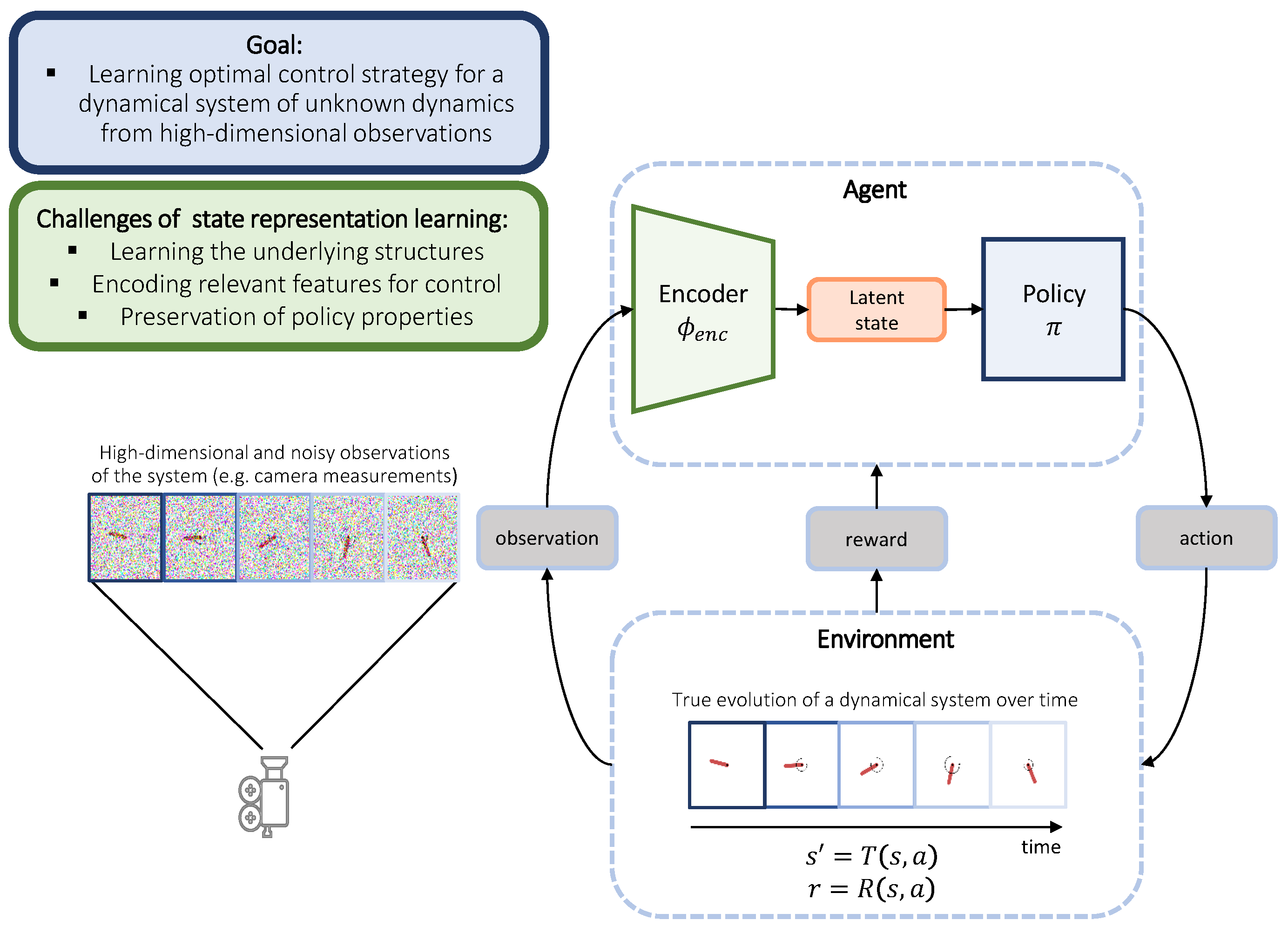
Figure 1: State Representation Learning for Deep Reinforcement Learning.

Inspired by the outstanding successes of Deep Learning (DL) [7], RL has turned towards deep function approximators, e.g. neural networks, for representing the control strategies and tackling the curse of dimensionality. The use of deep neural networks in RL gave birth to Deep Reinforcement Learning (DRL). DRL has achieved outstanding successes in learning optimal policies directly from high-dimensional observations [8, 9, 10]. However, neural networks’ drawbacks have also been inherited, namely the low sample efficiency, the consequent need for huge amounts of data, and the instabilities of learning.

The sample inefficiency of the methods is one of the significant drawbacks of DRL-based control. This aspect becomes even more severe when controlling dynamical systems requiring real-world interaction – we cannot afford our robots to collide with obstacles multiple times before learning how to navigate around them properly. The sample inefficiency of DRL derives from disregarding any prior knowledge of the world and the sole use of the reward signal to optimize the neural network models. The reward signal assesses only the quality of the decision but does not directly indicate the best course of action. It is worth highlighting that DRL does not rely on any labelled data as in the case of standard supervised learning. Therefore, DRL, to improve sample efficiency, has recently shifted its focus toward unsupervised learning of data representations [11].

In real-world control problems, we often do not have access to the state variables unequivocally describing the evolution of the systems. However, we only have access to indirect, high-dimensional, and noisy measurements – observations in DRL terminology – e.g. noisy RGB images or, in general, any given sensory data. While data are often high-dimensional, many dynamical systems exhibit low-dimensional behaviours that can be effectively described by a limited number of latent variables that capture the systems’ essential properties for control and identification purposes. Given the observation stream, we want to learn low-dimensional state representations that preserve the relevant properties of the world and eventually use such representations to learn the optimal policies. When DRL methods rely on compact representations, instead on high-dimensional observations, the algorithms gain higher sample efficiency, generalization and robustness. Figure 1 depicts how to exploit unsupervised representation learning in DRL in the context of control of dynamical systems, e.g. a simple pendulum. Again, we do not usually have access to the labelled data, i.e. the actual state values. Learning meaningful data representations for control without supervision is a significant and open challenge of DRL research, and it is often studied under the name of State Representation Learning (SRL) [12, 13, 14].

Our paper aims to provide a comprehensive and complete review of the most relevant, influential, and newest trends of unsupervised state representation learning in DRL. Other surveys from the literature, e.g. [12, 13, 14], although they cover a considerable amount of work, they are outdated considering the rapid evolution of the research in this field, and do not cover the latest discoveries. Our review:

• describes the main DL tools used in DRL for learning meaningful representations and their desired properties,

• classifies the important trends by analyzing the most relevant contributions in the field,

• summarizes the applications, benchmarks and evaluation strategies crucial for the advance of the research, and

• provides an elaborate discussion on open challenges and future research directions.

We review over 100 publications on a wide variety of approaches for unsupervised learning in DRL. We include papers from relevant journals conferences in the field (e.g. NIPS, ICRL, ICML, ICRA, and IROS) and ArXiv, and we checked each contribution’s references and related work. We identified the relevant contributions using keywords such as: "State Representation Learning", "Deep Reinforcement Learning", and "Learning Abstract Representations". The latest work included in the review is dated January 2022.

The review is organized as follows: Section Background provides the background information related to MDPs and the notation. Section Deep Learning for Learning State Representations provides a gentle introduction to the Deep Learning methods constituting the building blocks for learning meaningful representations. Section Unsupervised Representation Learning in Deep Reinforcement Learning describes the SRL methods from the literature and Section Advanced Methods and Applications describes the advanced methods and the most prominent applications of SRL. Section Evaluation and Benchmark discusses the evaluation metrics and the benchmarks. Section Discussion uses our experience in the field to discuss the open challenges and the most exciting research directions and Section Conclusion concludes the review.

2 Background

In Section Markov Decision Processes, we introduce the Markov Decision Processes (MDP) framework, in Section Partially Observable Markov Decision Processes the Partially Observable Markov Decision Processes (POMDP), and in Section Block MDP the Block Markov Decision Process (BMDP) framework. Eventually, in Section Notation, we introduce the notation used in SRL and this review.

2.1 Markov Decision Processes

The discrete time-steps agent-environment interaction scheme of RL can be studied by means of the MDPs.

Definition 1.

MDP. A finite MDP is a tuple $\langle\mathcal{S},\mathcal{A},T,R\rangle$ where $\mathcal{S}\subset\mathbb{R}^{n}$ is the set of states, $\mathcal{A}\subset\mathbb{R}^{m}$ is the set of actions, $T:\mathcal{S}\times\mathcal{S}\times\mathcal{A}\longrightarrow[0,1];\ (\bm{s}^{\prime},\bm{s},\bm{a})\longmapsto T(\bm{s}^{\prime},\bm{s},\bm{a})=p(\bm{s}^{\prime}|\bm{s},\bm{a})$ is the transition function, describing the probability $p(\bm{s}^{\prime}|\bm{s},\bm{a})$ of reaching state $\bm{s}^{\prime}$ from state $\bm{s}$ while taking action $\bm{a}$, and $R:\mathcal{S}\times\mathcal{A}\longrightarrow\mathbb{R};\ (\bm{s},\bm{a})\longmapsto R(\bm{s},\bm{a})$ is the reward function.

The goal of the agent is to find the optimal stochastic policy $\pi^{*}(\bm{a}|\bm{s})$, i.e. the policy maximizing the expected cumulative reward in the long run. Differently from Dynamic Programming [5], in RL the agent has no knowledge of the transition function $T$ and the reward function $R$ and has to learn the optimal behaviour by interacting with the environment.

2.2 Partially Observable Markov Decision Processes

In many real-world problems, the state of the environment is not directly accessible by the agent, and the world is only observable via partial and often high-dimensional observations. Examples of partial observable environments are: the Atari games [8] when played using pixel inputs, or a robot learning to navigate by relying only on sensory readings [15]. The MDP framework is insufficient for properly model these problems as a single observation may not be sufficient to distinguish between two or more states unequivocally. Therefore, one must rely on the framework of Partial Observable Markov Decision Process (POMDP).

Definition 2.

POMDP. A POMDP is a tuple $\langle\mathcal{S},\mathcal{A},\mathcal{O},T,\Omega,\mathcal{R}\rangle$ where $\mathcal{S}\subset\mathbb{R}^{n}$ is the set of unobsevables states, $\mathcal{A}\subset\mathbb{R}^{m}$ is the set of actions, $\mathcal{O}\subset\mathbb{R}^{o}$ is the set of observations, $T:\mathcal{S}\times\mathcal{S}\times\mathcal{A}\longrightarrow[0,1];\ (\bm{s}^{\prime},\bm{s},\bm{a})\longmapsto T(\bm{s}^{\prime},\bm{s},\bm{a})=p(\bm{s}^{\prime}|\bm{s},\bm{a})$ is the transition function, $\Omega:\mathcal{O}\times\mathcal{S}\times\mathcal{A}\longrightarrow[0,1];\ (\bm{o},\bm{s},\bm{a})\longmapsto\Omega(\bm{o},\bm{s},\bm{a})=p(\bm{o}|\bm{s},\bm{a})$ is the observation function and $R:\mathcal{S}\times\mathcal{A}\longrightarrow\mathbb{R};\ (\bm{s},\bm{a})\longmapsto R(\bm{s},\bm{a})$ is the reward function.

To learn the optimal policy, the agent must first infer its current state $\bm{s}_{t}$. Due to the partial observability of the environment, a single observation is not enough for discriminating between states. Thus, the state estimation problem $p(\bm{s}_{t}|\bm{o}_{t},\bm{o}_{t-1},\cdot,\bm{o}_{t-n})$ requires the history of observations. In the most general settings, the problem of learning state representation has to be modeled using the POMDP framework. However, in some cases, e.g. in [16], we can rely on a simplified version of such framework: the Block MDP (BMDP) [17].

2.3 Block MDP

In a BMDP [18], each observation has only one corresponding environment state and can be considered Markovian.

Definition 3.

BMDP. A BMDP with a tuple $\langle\mathcal{S},\mathcal{A},\mathcal{O},T,\Omega,\mathcal{R}\rangle$ where $\mathcal{S}$ is the set of unobservable states, $\mathcal{A}$ is the set of actions $\mathcal{O}$ observation space here assumed Markovian, $T:\mathcal{S}\times\mathcal{S}\times\mathcal{A}\longrightarrow[0,1];\ (\bm{s}^{\prime},\bm{s},\bm{a})\longmapsto T(\bm{s}^{\prime},\bm{s},\bm{a})=p(\bm{s}^{\prime}|\bm{s},\bm{a})$ is the transition function, $R:\mathcal{S}\times\mathcal{A}\longrightarrow\mathbb{R};\ (\bm{s},\bm{a})\longmapsto R(\bm{s},\bm{a})$ is the reward function, and $\Omega:\mathcal{O}\times\mathcal{S}\times\mathcal{A}\longrightarrow[0,1];\ (\bm{o},\bm{s},\bm{a})\longmapsto\Omega(\bm{o},\bm{s},\bm{a})=p(\bm{o}|\bm{s},\bm{a})$ is the observation function.

The advantage of modelling problems via BMDPs rather than POMDPs is that we do not need any memory structure for learning the state representation, as single observations already contain all the information for inferring the states, i.e. $p(\bm{s}_{t}|\bm{o}_{t})$. However, even when the observations are Markovian, encoding the relevant information from the high-dimensional and potentially noisy measurements to the latent states still remains a challenge.

2.4 Notation

In the most general case, a state representation $\bm{z}$ is a function of all the history of observations collected by the agent while interacting with the environment

$$\bm{z}_{t}=\phi_{\text{enc}}(\bm{o}_{t},\bm{o}_{t-1},\dots,\bm{o}_{0})\,,$$ (1)

where we refer to $\phi_{\text{enc}}$ as the encoder, $z_{t}$ is the latent state at time step $t$, and $o_{t},\dots,o_{0}$ indicate the observations from time step $t$ to $0$.

However, in practice, we rarely need the complete history, and only a subset of it is sufficient for inferring the state:

$$\bm{z}_{t}=\phi_{\text{enc}}(\bm{o}_{t},\dots,\bm{o}_{t-n})\,,$$ (2)

with $n<<t$.

In the case of BMDPs, the latent states depend only on the information at the current time step, i.e. no history is considered:

$$\bm{z}_{t}=\phi_{\text{enc}}(\bm{o}_{t})$$ (3)

For introducing and describing the SRL methods, in Section Unsupervised Representation Learning in Deep Reinforcement Learning, we will use the BMDPs notation for the sake of simplicity. However, the notation can be easily extended to sequences of observations:

$$\bm{z}_{t}=\phi_{\text{enc}}(\tilde{\bm{o}}_{t})\,,$$ (4)

with $\tilde{\bm{o}}_{t}=\bm{o}_{t,t-1,\dots,t-n}$ respectively.

Remark: In practice, many of the methods we reviewed use auxiliary models, e.g. forward or reward models, for generating informative gradients for the training of $\phi_{\text{enc}}$. Thus, the latent states are also function of the (sequence of) actions and rewards.

In this review, we specifically focus on the methods relying on Deep Learning [7] and neural networks for approximating the unknown function $\phi_{\text{enc}}$.

3 Deep Learning for Learning State Representations

This section is composed of three parts: (i) we introduce the basic neural network architectures in Section Neural Network Architectures that can be used to approximate the mapping $\phi_{\text{enc}}$ (see Equation (4)), (ii) we show different unsupervised learning methods for learning the optimal mapping $\phi_{\text{enc}}$ in Section State Representation Learning Methods, and (iii) we summarize and discuss the methods introduced in Section Summary.

3.1 Neural Network Architectures

3.1.1 Fully-Connected Neural Networks

Fully-Connected neural networks (FCNNs) [19] lay the foundations of Deep Learning (DL). FCNNs are a family of parametric models used to approximate any unknown function $f:\mathcal{X}\longrightarrow\mathcal{Y};\bm{x}\longmapsto f(\bm{x})$ by means of a parametric function $\phi$ such that $\bm{y}=\phi(\bm{x};\bm{\theta})$. The neural network parameters $\bm{\theta}\in\mathbb{R}^{t}$ are optimized, via a training set of examples and gradient descent, to find the best approximation of $f$. An example of a two-layer FNN is shown in Figure 2.

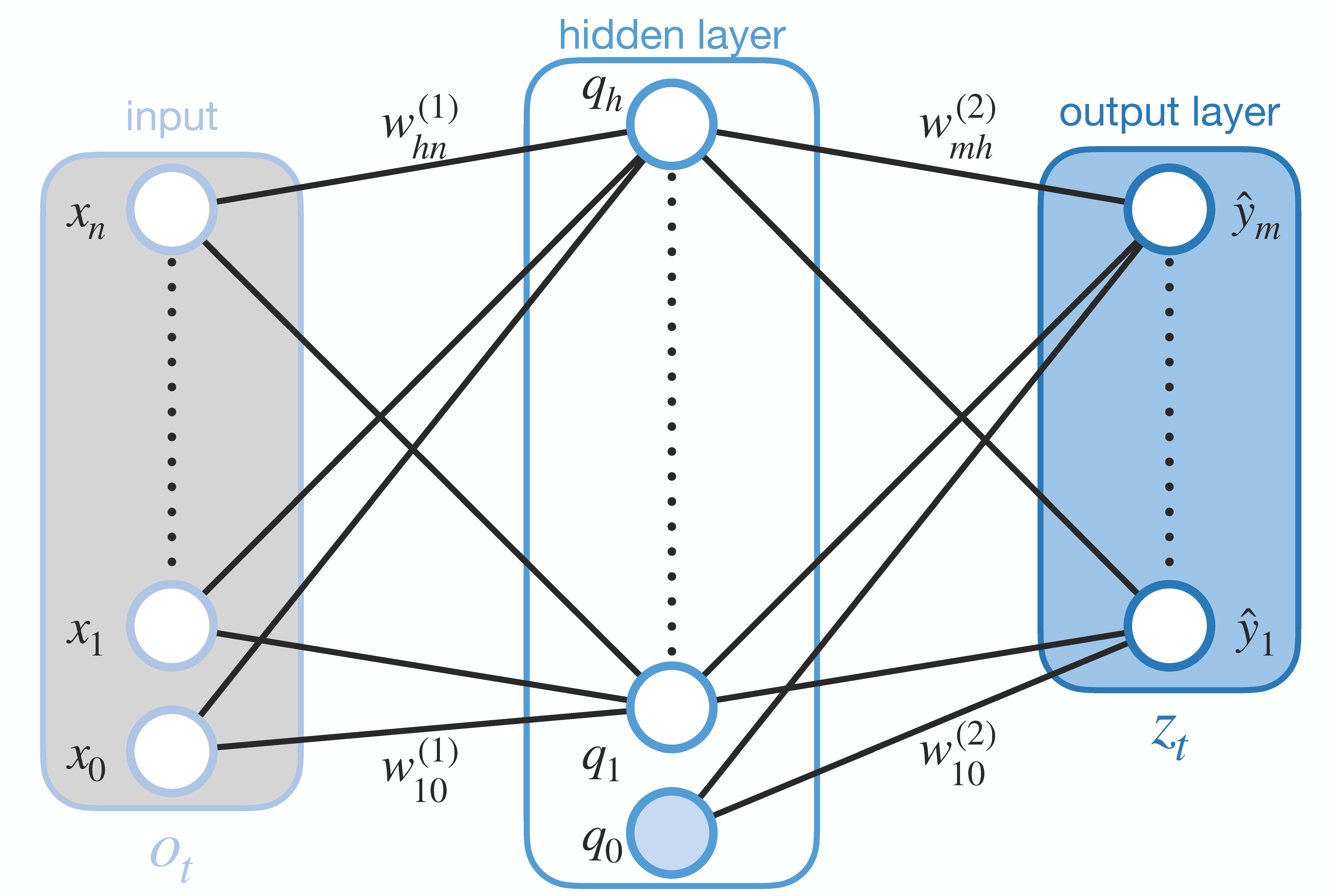
Figure 2: Two-layers feedforward neural networks with $n$ inputs, $h$ hidden neurons and $m$ outputs. The input and output are indicated with $\bm{x}$, and $\bm{y}$, the weights of the network are indicated with $w$ (e.g. $w^{(1)}_{hn}$ corresponds to the weight of the first layer connecting $n^{th}$-input to the $h^{th}$-hidden node) and the biases with the subscript $0$. In the context of SRL, the input is none other than the observation $\bm{o}_{t}$ while the output is the latent state $\bm{z}_{t}$. Figure reproduced and adapted from [20].

Assuming the FCNN depicted in Figure 2 with $n$ inputs, $h$ hidden neurons, or nodes, $m$ outputs, a set weights and biases $\bm{\theta}$, i.e. the parameters, and an activation function $\xi(\cdot)$, we can define the contribution of the $i^{th}$-component of the input $x_{i}$ to the $k^{th}$-component of the output $y_{k}$ as:

$$\begin{split}a_{j}&=\sum^{n}_{i=1}w^{(1)}_{ji}x_{i}+w^{(1)}_{j0}\\ q_{j}&=\xi(a_{j})\\ a_{k}&=\sum^{h}_{j=1}w^{(2)}_{kj}q_{j}+w^{(2)}_{k0}\\ y_{k}&=\xi(a_{k})\\ \end{split}$$ (5)

If the activation function $\xi(\cdot)$ is chosen linear, the output is a linear combination of the inputs. However, in most cases, the activation function is chosen nonlinear. FCNNs with nonlinear activations are universal function approximators [21]. Common activation functions are sigmoid, tanh, rectified linear unit (ReLU), and softmax.

Independently of the structure of the network, we need a way to learn the parameters $\bm{\theta}$, i.e. weights $w_{i}$ and biases $b_{i}$, of the network to best approximate the unknown target function $f$, given a set of training samples. We can do this by means of gradient descent and back-propagation by choosing a suitable loss, or cost function $\mathcal{L}$.

For example, consider the SRL problem in Supervised Learning settings, we are given a training set of input data $\bm{x}^{(1)},\dots,\bm{x}^{(l)}$, target values $\bm{y}^{(1)},\dots,\bm{y}^{(l)}$, and the set of predicted values $\hat{\bm{y}}^{(1)},\dots,\hat{\bm{y}}^{(l)}$, where $\hat{\bm{y}}^{(i)}=\phi(\bm{x}^{(i)};\bm{\theta})$. We can compute the prediction errors of the neural network $\phi$ and adjust the network parameters to minimize such errors. A commonly used loss function is the mean square error (MSE) loss over the training set, as shown in Equation (6)).

$$\begin{split}\min_{\bm{\theta}}&\ \ \ \ \mathcal{L}(\bm{\theta})\\ \mathcal{L}(\bm{\theta})&=\frac{1}{l}\sum^{l}_{i=1}\mid\mid\bm{y}^{(i)}-\phi(\bm{x}^{(i)};\bm{\theta})\mid\mid^{2}\\ &\approx\mathbb{E}_{\bm{x},\bm{y}\sim\mathcal{D}}\mid\mid\bm{y}-\phi(\bm{x};\bm{\theta})\mid\mid^{2}\,,\\ \end{split}$$ (6)

where $l$ is the number of data in the training set, $\bm{y}^{(i)}$ is the $i^{th}$ target output data, $\phi(\bm{x}^{(i)};\bm{\theta})$ is the predicted output given the input $\bm{x}^{(i)}$, and we assume the input and output data, $\bm{x}^{(1)},\dots,\bm{x}^{(l)}$ and $\hat{\bm{y}}^{(1)},\dots,\hat{\bm{y}}^{(l)}$ respectively, to be sampled from the empirical distribution of the training set $\mathcal{D}$. At each training operation, we compute the gradient $\nabla_{\bm{\theta}}\mathcal{L}(\bm{\theta})$ concerning the network parameters and then back-propagate this gradient through each layer and neuron from output to input. Computing the expectation over the whole training dataset $\mathbb{E}_{\bm{x},\bm{y}\sim\mathcal{D}}$ is usually expensive in terms of computations and hardware resources. Thus, a random subset of data, i.e. a minibatch, is used to train the neural networks. For more details on back-propagation and optimization methods for training deep neural networks, we refer the reader to [19].

Unfortunately, in the context of SRL, we cannot rely on the true states $\bm{s}$ and directly perform regression. However, we must use auxiliary models to learn the encoder’s parameters. We will discuss this aspect in Section Observation Reconstruction-Contrastive Learning.

3.1.2 Convolutional Neural Networks

Convolutional neural networks (CNNs) [22] are neural networks specialised in efficiently handling data with grid-like structure, e.g. images (2D pixel grids) or LiDAR readings (1D data grids). CNNs inherit their name from the mathematical operator they employ in at least one of their layers, i.e. the convolution.

For example, given a sequence of 1D noisy sensor reading measuring the position of a robot over time $\bm{x}(t)$ with $t\in(-\infty,\infty)$, we would like to obtain a better estimate of the robot position $\bm{x}(t)$ by averaging multiple measurements over time. However, past measurements’ contribution should depend on the time instant the measurements are obtained, and older measurements should be trusted less than the newer ones. Therefore, to find a smooth estimate of the robot pose, we need a weighting function $K(a)$ dependent on the age $a$ of the measurements we need to apply for each time instant $t$. The function $K$ is usually called kernel or filter. This whole operation is called convolution and is indicated by $*$. In general, we deal with computers and sensors providing data at discrete time steps, and the smoothed position of the robot $\bm{x}_{s}(t)$ can be expressed as:

$$\bm{x}_{s}(t)=(\bm{x}*K)(t)=\sum^{t}_{a=-\infty}x(a)K(t-a)$$ (7)

We can also use the convolution operator over multi-dimensional inputs, but in particular, we are interested in using convolutions for the special case of 2D inputs, e.g. images. Given a 2D image $I$ of size $m\times n$ and a 2D kernel $K$, the convolution operation of sliding the kernel over the image can be defined as:

$$S(i,j)=(I*K)(i,j)=\sum^{m}_{i=1}\sum^{n}_{j=1}I(m,n)K(i-m,j-n)$$ (8)

After defining the convolution operator, we want to understand how it is used in CNNs and the advantages of FCNNs. First, unlike FCNNs that use full connectivity of each input and output neuron, CNNs are an example of sparse connectivity when the kernel size is smaller than the input data size. Convolution allows reducing the number of network parameters, the physical memory required to store it and the number of computations for computing the outputs.

In a convolutional layer of a neural network, we can identify:

• Apply convolution to generate activations (see Figure 3)

• Pass the activations through non-linear activation functions (e.g. ReLU)

• Apply pooling to change (reduce) the shape of the output of the layer

The trainable parameters of CNNs are the elements of the kernels. These parameters can be learned with the same approach used by FCNNs by defining a loss function and adjusting the network parameters according to its gradient with respect to the parameters, i.e. via back-propagation. By learning the weights of the kernels, it is possible to identify different features of the input data, for example, edges and shapes in the case of 2D images. CNNs employ parameter sharing to reduce the number of parameters with respect to FCNNs. Multiple kernels are slid with a certain stride length across the whole data grid to extract different features. Figure 3 shows an example of convolution applied to an image. It is worth highlighting that, because of parameter sharing, CNN are shift equivariant – applying a shift transformation to the image before applying the convolution operator (see (8)) is equivalent to applying the convolution and then the shift transformation. As with FCNNs, multiple convolutional layers can be stacked together. The more the convolutional layer is close to the network’s output, the higher the level of abstraction of the learned features (e.g., edges and colours to more complex shapes).

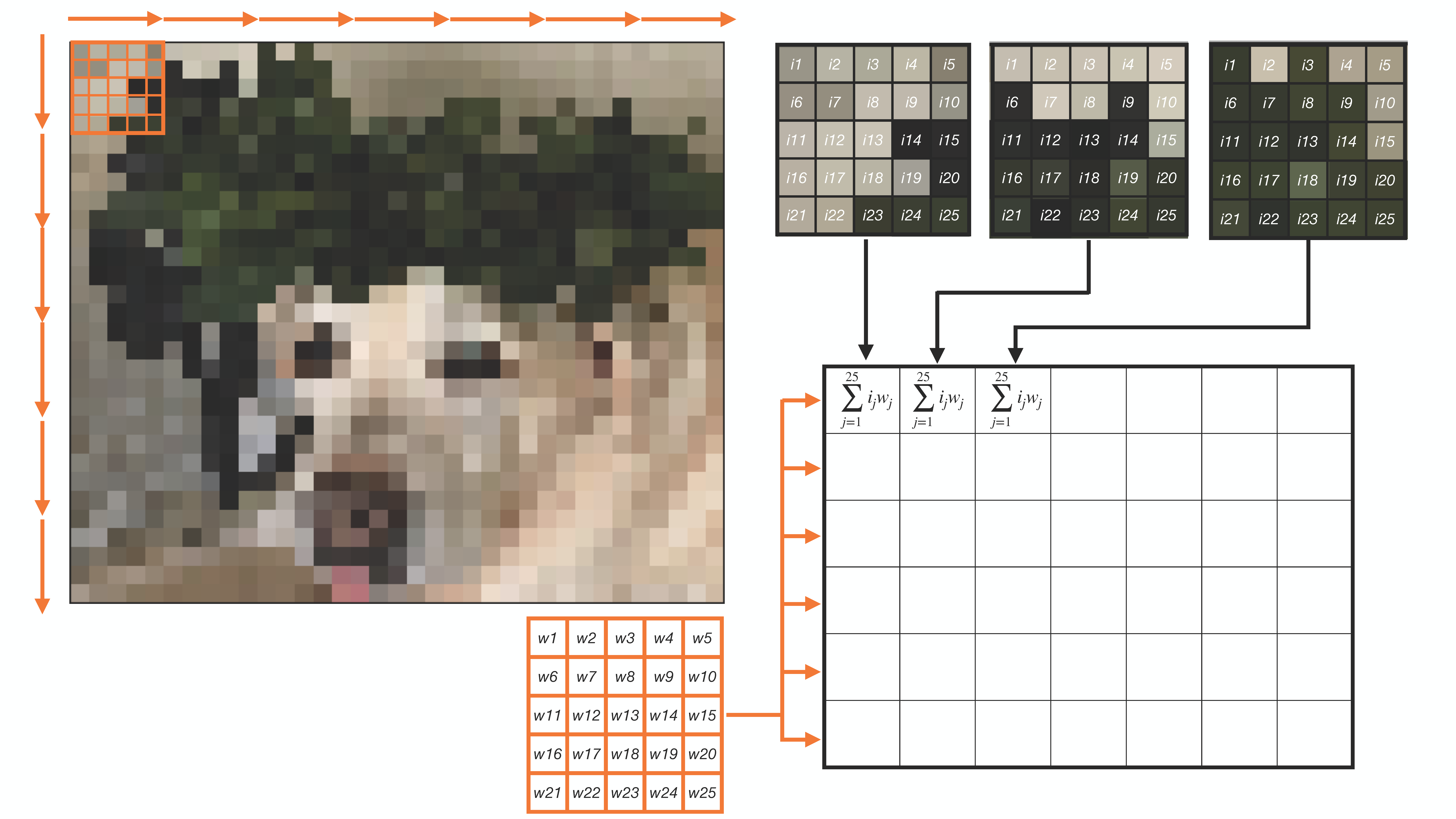
Figure 3: Example of 2D-convolution with a kernel with size $5\times 5$ and stride $5$. Figure reproduced from [20].

The most widely-studied example of using CNNs is probably the problem of classifying images. Given a training set of labelled images (e.g. a data set containing images of dogs and cats and the correct labels), the neural network has to learn to properly determine if the input images belong to one of the data classes. Therefore, the network must learn to extract each class’s representative features to distinguish among them.

In the context of SRL, we often deal with image observation. Therefore CNNs are fundamental architectures for extracting the relevant features, lightening the computational burden of FCNNs, and effectively reducing the dimensionality.

3.1.3 Recurrent Neural Networks

Recurrent neural networks (RNNs) [23] are the class of neural networks specialized in handling sequences of data with either fixed or variable length. RNNs can be used in different contexts, for example, to map sequences to sequences, e.g. in natural language processing, or sequences to a single outputs, e.g. for solving POMDP in DRL and SRL.

Similar to the case of FCNNs, we can analytically define the relation between the input vector $\bm{x}$, the hidden state vector $\bm{h}$ and the predicted output $\hat{\bm{y}}$ as:

$$\begin{split}\bm{a}_{t}&=W\bm{h}_{t-1}+U\bm{x}_{t}+\bm{b}\\ \bm{h}_{t}&=\xi(\bm{a}_{t})\\ \hat{\bm{y}}_{t}&=V\bm{y}_{t}+\bm{c}\,,\\ \end{split}$$ (9)

where $W,U,V$ are the weight matrices and $\bm{b},\bm{c}$ are the bias vectors.

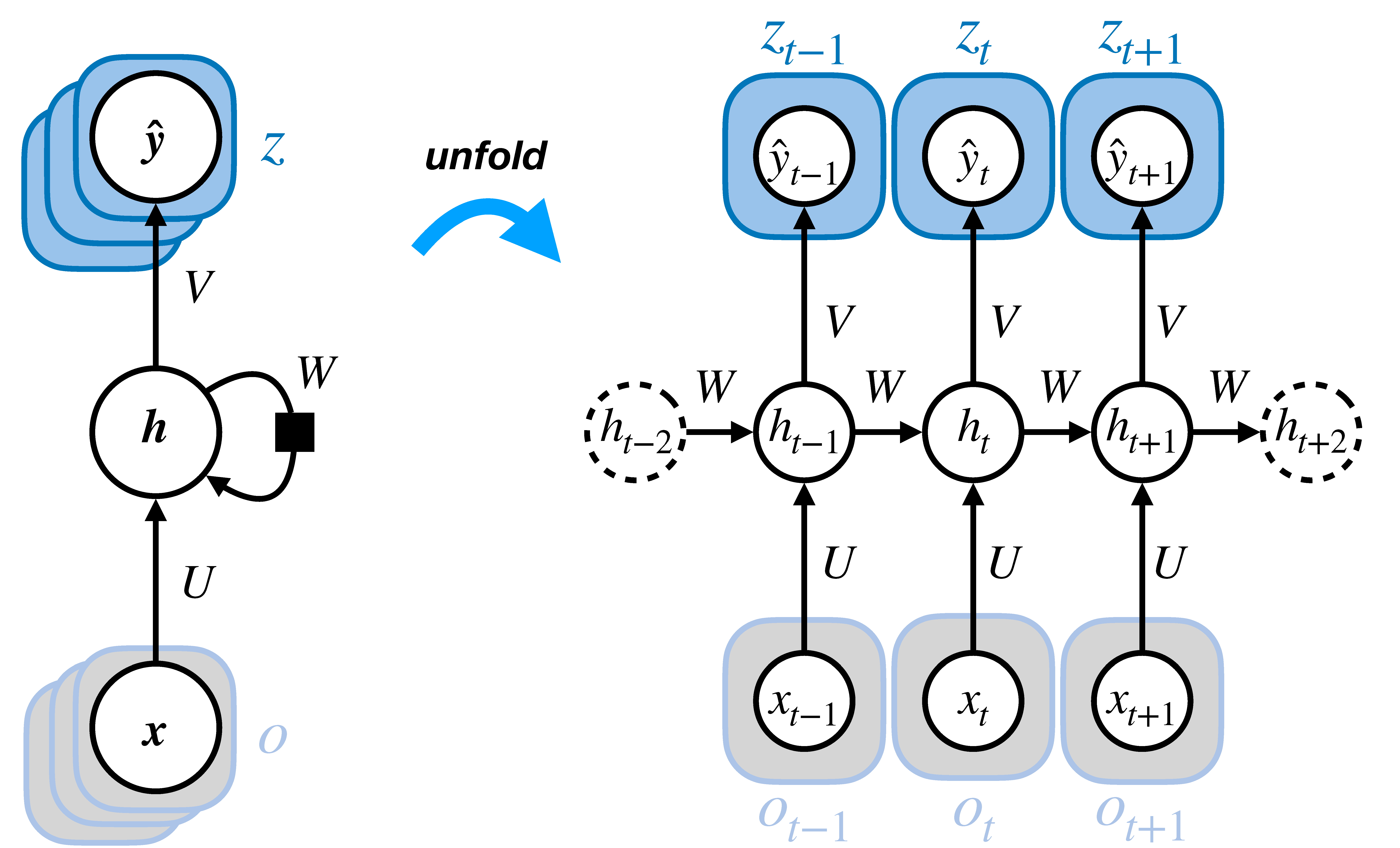
Figure 4: Computational graph of a recurrent neural network. Figure reproduced and adapted from [20].

Similarly to FCNNs and CNNs, RNNs are trained by defining a loss function and by applying back-propagation. A widely-used RNN architecture is the Long-Short Term Memory (LSTM) [24] using a sophisticated gating mechanism for preventing the vanishing of the gradient problem that affects the simple RNN architecture.

3.1.4 Neural Networks in State Representation Learning

FCNNs, CNNs, and RNNs form the building blocks for parametrizing the unknown mapping $\phi_{\text{enc}}$ encoding observations from the world into a low-dimensional latent state space that can be used to learn the optimal behaviour. The neural network architecture has to be chosen depending on the MDP type and that data structure. In Figure 5, we depict the four most used neural network architectures from the literature, in the case of MDPs, BMDPs or POMDPs and if grid-structured data are used or not.

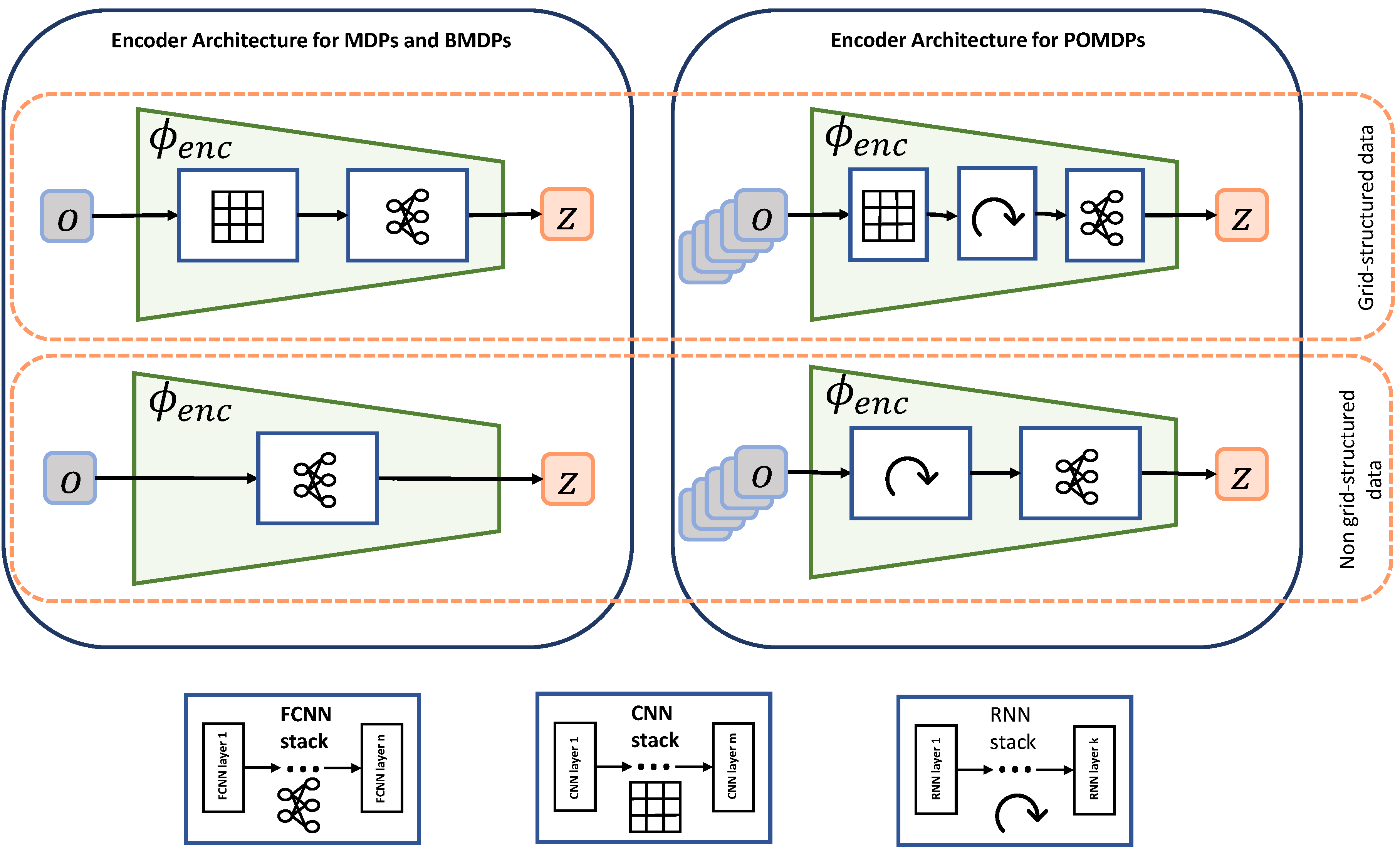
Figure 5: Neural network architectures of the encoder $\phi_{\text{enc}}$ in MDP, BMDP, and POMDPs in the presence of grid-structured and non-grid-structured data. FCNNs are indicated by the graph symbol, CNNs by the matrix grid, and RNNs by the looping arrow. The encoder $\phi_{\text{enc}}$ can be either deterministic, i.e. $\bm{z}=\phi_{\text{enc}}(\bm{o})$, or stochastic, i.e.$\bm{z}\sim p(\bm{z}|\bm{o})=\phi_{\text{enc}}(\bm{o})$.

3.2 State Representation Learning Methods

Before diving into the methods, we introduce and discuss the properties of the state representations we aim at learning in Section Properties of the Learned State Representations. The rest section is articulated in four main blocks:

• Section Observation Reconstruction we describe the approaches for SRL based on Principal Components Analysis (PCA) [25] and observation reconstruction [26, 27],

• Section Latent MDP models presents the MDP models and describes their usage as auxiliary models for encoding observations into a low-dimensional latent state space,

• Section Priors discusses the so-called Robotics Priors [28], and

• Section Contrastive Learning focuses on contrastive losses [29].

These four blocks will be a recurring theme in the rest of the review.

3.2.1 Properties of the Learned State Representations

Analogously to DL, learning compact and meaningful representation is crucial for the performance of the algorithms. In DRL, the benefits are several:

• Sample efficiency. Fast learning from limited data samples is fundamental to DRL’s progress. For example, in robotics, we have limited access to real-world data while we need to learn complicated behaviours.

• Robustness. Due to the dimensionality reduction and the embedding in lower-dimensional spaces, we are less prone to overfitting and noise.

• Generalization. By encoding and disentangling the critical factor for explaining the world from the irrelevant ones, good representations are more prone to generalize to new environments with similar features.

• Interpretability. Latent representations are often composed of interpretable features and can often be visualized in 2D or 3D plots.

In the most general case of a POMPD, the goal is to encode each sequence of high-dimensional observations into a latent state space $\mathcal{Z}$ containing all the relevant information for optimally and efficiently learning to solve the task. In the case of a BMDP, we encode single observations to infer the latent states. Here, we discuss which are the desired properties for $\mathcal{Z}$, according to [11, 12, 13]:

1. $\mathcal{Z}$ should be smooth. If $\bm{o}_{t_{1}}\approx\bm{o}_{t_{2}}$, then $\phi_{\text{enc}}(\bm{o}_{t_{1}})\approx\phi_{\text{enc}}(\bm{o}_{t_{2}})$, then our representation can generalize to similar features.

2. $\mathcal{Z}$ should be a low-dimensional manifold. The latent states are concentrated in a region of much smaller dimensionality than the observation space.

3. elements in $\mathcal{Z}$ should represent the complex dependencies arising from the study of complex systems, possibly in a simple manner, i.e. the transition function between latent states should be a relatively simple (quasi-linear) transformation.

4. $\mathcal{Z}$ should be Markovian. An RL algorithm without memory should be able to solve the problem using the state representation optimally.

5. $\mathcal{Z}$ should be temporally coherent. Consecutive observations should be mapped closer in the latent space than non-consecutive ones.

6. $\mathcal{Z}$ should be sufficiently expressive and contain enough information to allow the agent to learn the optimal policy.

We will link these properties to the methods in Section Summary.

3.2.2 Observation Reconstruction

Assuming a high-dimensional observation space, one can think of projecting the observations into a lower-dimensional space. The projection must maintain all (most of) the relevant information while discarding the irrelevant ones. This process can be done by considering the covariance matrix of the data, computing the eigenvalues and projecting the dataset in the lower-dimensional space defined by the $n$ eigenvalues with the highest variance, i.e. the eigenvalues better explaining the data. This procedure is called Principal Component Analysis (PCA) [25].

One of the drawbacks of PCA is that the data are linearly projected into a low-dimensional space. However, this hinders its application to cases where no linear mapping exists between observations and latent states, and a nonlinear complex mapping has to be learned.

Autoencoders (AEs) [26] are neural networks composed of an encoder $\phi_{\text{enc}}$, with parameters $\bm{\theta}_{\text{enc}}$, and a decoder $\phi_{\text{dec}}$, with parameters $\bm{\theta}_{\text{dec}}$. The encoder maps the input data $\bm{o}_{t}$ to a low-dimensional latent representation or abstract code $\bm{z}_{t}=\phi_{\text{enc}}(\bm{o}_{t};\bm{\theta}_{\text{enc}})$, while the decoder reconstructs the input signal $\hat{\bm{o}}_{t}=\phi_{\text{dec}}(\bm{z}_{t};\bm{\theta}_{\text{dec}})$ given the latent representation $\bm{z}_{t}$, see Figure 6.

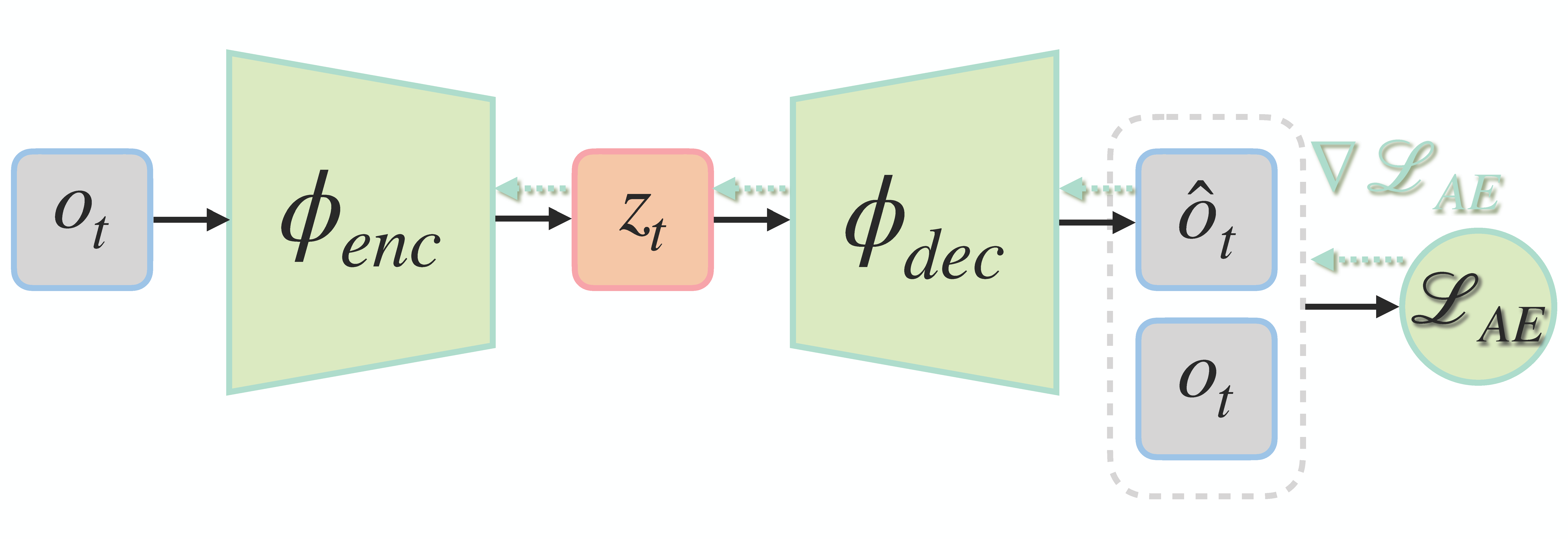
Figure 6: Autoencoder architecture.

The low-dimensionality of the latent representations is a form of regularisation for preventing the learning of the trivial identity mapping. For more information, we refer the reader to [11].

The AE is trained by minimizing the so-called reconstruction loss, i.e. the Mean Squared Error loss between the original input and the reconstructed one, as shown in Equation (10)).

$$\begin{split}\min_{\bm{\theta}_{\text{enc}},\bm{\theta}_{\text{dec}}}&\ \ \ \ \mathcal{L}_{AE}(\bm{\theta}_{\text{enc}},\bm{\theta}_{\text{dec}})\\ \mathcal{L}_{AE}(\bm{\theta}_{\text{enc}},\bm{\theta}_{\text{dec}})&=\mathbb{E}_{\bm{o}_{t}\sim\mathcal{D}}[\mid\mid\bm{o}_{t}-\hat{\bm{o}}_{t}\mid\mid^{2}]\\ &=\mathbb{E}_{\bm{o}_{t}\sim\mathcal{D}}[\mid\mid\bm{o}_{t}-\phi_{\text{dec}}(\bm{z}_{t};\bm{\theta}_{\text{dec}})\mid\mid^{2}]\\ &=\mathbb{E}_{\bm{o}_{t}\sim\mathcal{D}}[\mid\mid\bm{o}_{t}-\phi_{\text{dec}}(\phi_{\text{enc}}(\bm{o}_{t};\bm{\theta}_{\text{enc}});\bm{\theta}_{\text{dec}})\mid\mid^{2}]\,,\end{split}$$ (10)

where $\bm{o}_{t}$ is the original input observation, $\hat{\bm{o}}_{t}$ is its reconstruction using the AE, and $\mathcal{D}$ is the memory buffer containing the collected samples.

In DRL, the encoder of the AE is used to learn state representations from high-dimensional observations. Inputs can be either single observations, e.g. in BMDPs, or sequences of observations, e.g. in POMDPs. The latent state variables are then used to learn policies and value functions.

In the presence of uncertainties, AEs may be replaced with variational autoencoders (VAEs) [27]. Similarly to AEs, VAEs are also composed of an encoder and a decoder. However, differently from AEs, the latent space is modelled as a Normal distribution $\mathcal{N}(\bm{\mu}_{t},\Sigma_{t})$ with the encoder learning its statistics $\bm{\mu}_{t}$ and $\Sigma_{t}$ given an observation $\bm{o}_{t}$. The latent state $\bm{z}_{t}$ is sampled from $\mathcal{N}(\bm{\mu}_{t},\Sigma_{t})$, often using the so-called reparametrization trick [27]. Analogously to the case of an AE, $\bm{z}_{t}$ is then decoded via $\phi_{\text{dec}}$ to reconstruct the input observation $\hat{\bm{o}}_{t}$. The VAE architecture is depicted in Figure 7.

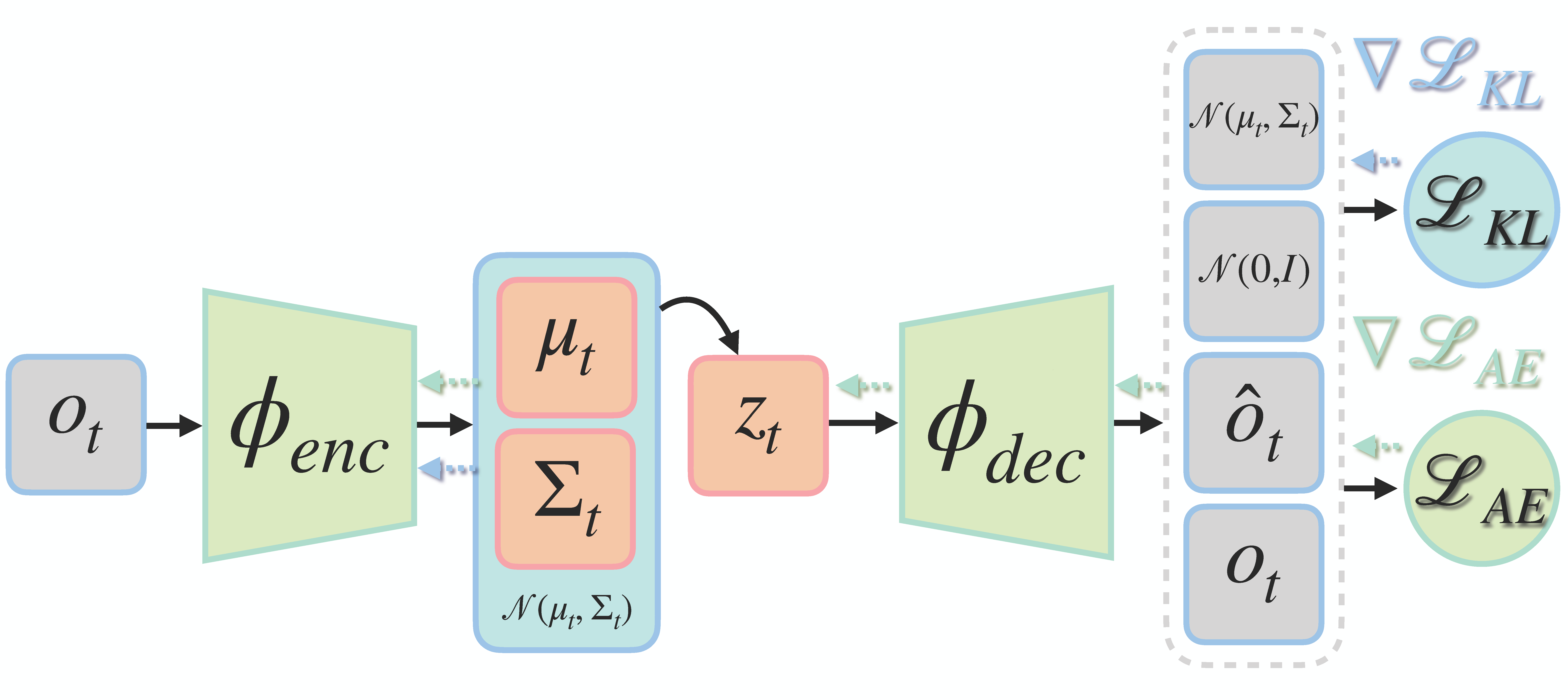
Figure 7: Variational autoencoder architecture.

The VAE loss function, shown in Equation (11), is composed of two terms: a reconstruction loss, similar to the AE, e.g. maximum likelihood, and a regularization term to enforce that the latent state distribution $\mathcal{N}(\bm{\mu}_{t},\Sigma_{t})$ is close to the Normal distribution $\mathcal{N}(\bm{0},I)$ using the Kullbach-Leibler divergence (KL).

$$\begin{split}\min_{\bm{\theta}_{\text{enc}},\bm{\theta}_{\text{dec}}}&\ \ \ \ \mathcal{L}_{AE}(\bm{\theta}_{\text{enc}},\bm{\theta}_{\text{dec}})+\mathcal{L}_{KL}(\bm{\theta}_{\text{enc}})\\ \mathcal{L}_{AE}(\bm{\theta}_{\text{enc}},\bm{\theta}_{\text{dec}})&=\mathbb{E}_{\bm{o}_{t}\sim\mathcal{D}}[-\log\phi_{\text{dec}}(\bm{o}_{t}|\bm{z}_{t};\bm{\theta}_{\text{enc}},\bm{\theta}_{\text{dec}})]\\ \mathcal{L}_{KL}(\bm{\theta}_{\text{enc}})&=\mathbb{E}_{\bm{o}_{t}\sim\mathcal{D}}[\text{KL}(\mathcal{N}(\bm{\mu}_{t},\Sigma_{t})||\mathcal{N}(\bm{0},I);\bm{\theta}_{\text{enc}})]\\ \end{split}$$ (11)

A commonly used variation of the VAE framework is the so-called $\beta$-VAE [30]. $\beta$-VAEs are special VAEs aiming to learn representations that disentangle the underlying factors of variation. This can be done by introducing a parameter $\beta$ in the loss function in Equation (11) as follows:

$$\begin{split}\min_{\bm{\theta}_{\text{enc}},\bm{\theta}_{\text{dec}}}&\ \ \ \ \mathcal{L}_{AE}(\bm{\theta}_{\text{enc}},\bm{\theta}_{\text{dec}})+\beta\mathcal{L}_{KL}(\bm{\theta}_{\text{enc}})\,,\\ \end{split}$$ (12)

where $\beta>1$ limits the capacity of the encoder and promotes the learning of disentangled representations.

The major flaw of the observation-reconstruction methods is intrinsic in the reconstruction loss itself, see Equation (10)-(12). The loss does not enforce any discrimination among features relevant for the control and features that are irrelevant. For example, images may contain many features, such as background textures, that are not relevant for learning the optimal policy, yet crucial for minimizing the reconstruction loss.

3.2.3 Latent MDP models

The state representations we seek to learn in DRL must include all the relevant information for learning to make optimal decisions. Therefore, learning approaches for SRL have to be able to discriminate between task-relevant and task-irrelevant features.

Instead of relying only on observation reconstruction, we can focus on encoding the relevant features for predicting the evolution of the world in the latent state space: the MDP models. The MDP models include the forward or transition model predicting the next state given the current one and the action taken, the reward model predicting the reward given the current state and action taken, and the inverse model predicting the action between pairs of consecutive states.

In the context of state representation learning, the MDP models act on latent state variables to describe the latent dynamics of the systems. Because these models utilize latent variables, we refer to them as latent MDP models. Figure 8 shows an example of a latent forward model. However, good latent MDP models are generally hard to learn, especially from high-dimensional noisy inputs.

In the following paragraphs, we explicitly focus on the latent forward model, the latent reward model, and the latent inverse model. These latent models are learned using the tuples $(\bm{o}_{t},\bm{a}_{t},\bm{o}_{t+1},r_{t})$ from the memory buffer. Then, we discuss different combinations of the MDP models that lay the foundation of two important theoretical frameworks in DRL: the MDP homomorphism and the bisimulation metric.

The latent forward model $T$ aims to describe the system’s forward evolution by predicting the next latent state $\bm{z}_{t+1}$ from the current latent state $\bm{z}_{t}$ and action $\bm{a}_{t}$. Depending on the context, the forward model can be either deterministic, i.e. $\bm{z}_{t+1}=T(\bm{z}_{t},\bm{a}_{t})$, or stochastic.

In deterministic settings, see Figure 8, the latent forward model $T$ maps $\bm{z}_{t}=\phi_{\text{enc}}(\bm{o}_{t};\bm{\theta}_{\text{enc}})$ and $\bm{a}_{t}$ to $\bm{z}_{t+1}=T(\bm{z}_{t},\bm{a}_{t};\bm{\theta}_{T})$.

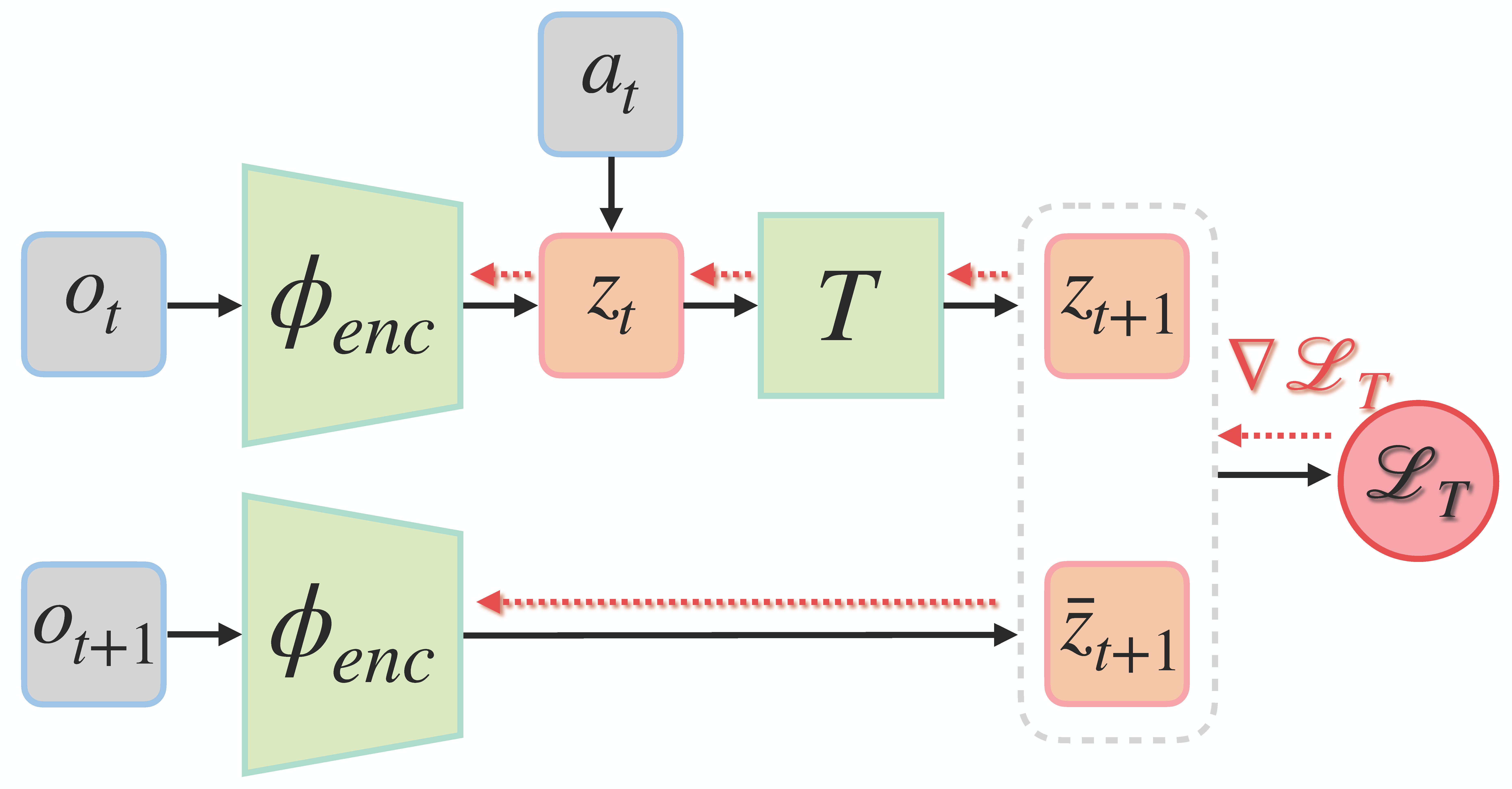
Figure 8: Latent forward model. The solid line represents the forward pass of the data through the networks, while the dashed lines the gradient flow.

The latent forward model can be used, and it is in practice often used, to compute an auxiliary loss whose gradients are employed to train the encoder $\phi_{\text{enc}}$. The loss, for the deterministic formulation of the models, is shown in Equation (13).

$$\begin{split}\min_{\bm{\theta}_{\text{enc}},\bm{\theta}_{T}}&\ \ \ \ \mathcal{L}_{T}(\bm{\theta}_{\text{enc}},\bm{\theta}_{T})\\ \mathcal{L}_{T}(\bm{\theta}_{\text{enc}},\bm{\theta}_{T})&=\mathbb{E}_{\bm{o}_{t},\bm{a}_{t},\bm{o}_{t+1}\sim\mathcal{D}}[\mid\mid\bar{\bm{z}}_{t+1}-\bm{z}_{t+1}\mid\mid^{2}]\\ &=\mathbb{E}_{\bm{o}_{t},\bm{a}_{t},\bm{o}_{t+1}\sim\mathcal{D}}[\mid\mid\phi_{\text{enc}}(\bm{o}_{t+1};\bm{\theta}_{\text{enc}})-T(\bm{z}_{t},\bm{a}_{t};\bm{\theta}_{T})\mid\mid^{2}]\\ &=\mathbb{E}_{\bm{o}_{t},\bm{a}_{t},\bm{o}_{t+1}\sim\mathcal{D}}[\mid\mid\phi_{\text{enc}}(\bm{o}_{t+1};\bm{\theta}_{\text{enc}})-T(\phi_{\text{enc}}(\bm{o}_{t};\bm{\theta}_{\text{enc}}),\bm{a}_{t};\bm{\theta}_{T})\mid\mid^{2}]\,,\end{split}$$ (13)

where the target next latent state $\bar{\bm{z}}_{t+1}=\phi_{\text{enc}}(\bm{o}_{t+1};\bm{\theta}_{\text{enc}})$ is generated by encoding the next observation $\bm{o}_{t+1}$, while $\bm{z}_{t+1}=T(\bm{z}_{t},\bm{a}_{t};\bm{\theta}_{T})$ is the predicted next latent state given the current observation $\bm{o}_{t}$ and the action taken $\bm{a}_{t}$.

Because the target next state $\bar{\bm{z}}_{t+1}$ is not known and generated by the same encoder, the representation may collapse to trivial embeddings. To prevent this issue other auxiliary losses such as contrastive losses have to be used [31, 32, 33]. We discuss contrastive losses in Section Contrastive Learning.

To encode task-relevant information into the state representation, we can make use of a latent reward model $R$ to predict the reward $\hat{r}_{t}=R(\bm{z}_{t},\bm{a}_{t})$ of a latent state-action pair $(\bm{z}_{t},\bm{a}_{t})$ (see Figure 9).

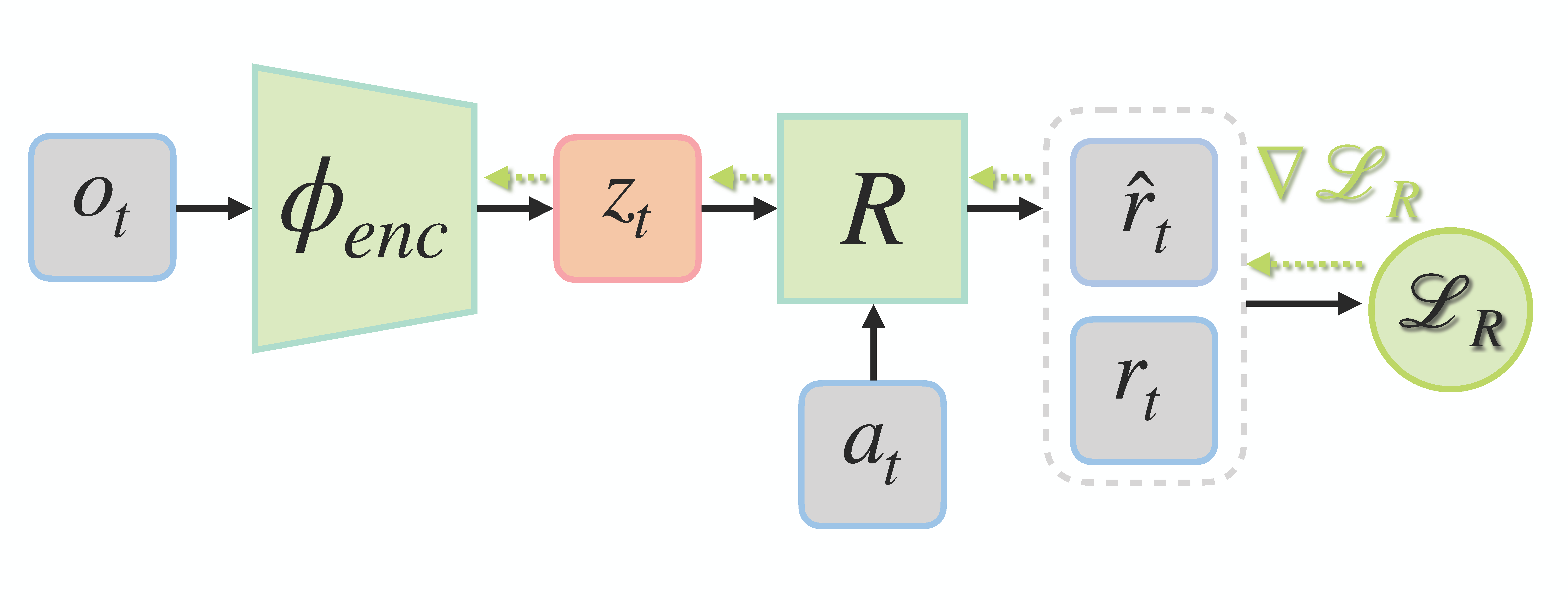
Figure 9: Latent Reward Model. The solid line represents the forward pass of the data through the networks, while the dashed lines the gradient flow.

The reward model utilizes the reward samples $r_{t}$ as target values for regression. In the deterministic case, an example of reward model loss is shown in Equation (14)).

$$\begin{split}\min_{\bm{\theta}_{\text{enc}},\bm{\theta}_{R}}&\ \ \ \ \mathcal{L}_{{R}}(\bm{\theta}_{\text{enc}},\bm{\theta}_{R})\\ \mathcal{L}_{{R}}(\bm{\theta}_{\text{enc}},\bm{\theta}_{R})&=\mathbb{E}_{\bm{o}_{t},\bm{a}_{t},r_{t}\sim\mathcal{D}}[\mid\mid r_{t}-\hat{r}_{t}\mid\mid^{2}]\\ &=\mathbb{E}_{\bm{o}_{t},\bm{a}_{t},r_{t}\sim\mathcal{D}}[\mid\mid r_{t}-R(\bm{z}_{t},\bm{a}_{t};\bm{\theta}_{R})\mid\mid^{2}]\\ &=\mathbb{E}_{\bm{o}_{t},\bm{a}_{t},r_{t}\sim\mathcal{D}}[\mid\mid r_{t}-R(\phi_{\text{enc}}(\bm{o}_{t};\bm{\theta}_{\text{enc}}),\bm{a}_{t};\bm{\theta}_{R})\mid\mid^{2}]\,,\end{split}$$ (14)

where $r_{t}$ is the reward sample from the memory buffer $\mathcal{D}$, and $\hat{r}_{t}=R(\bm{z}_{t},\bm{a}_{t};\bm{\theta}_{R},\bm{\theta}_{\text{enc}})$ is the reward predicted by the reward model $R$, parametrized by a neural network with parameters $\bm{\theta}_{R}$.

However, in the case of sparsity of the reward function, i.e. sparse rewards, the reward model alone may not be sufficient to learn a good representation as we may not be able to generate sufficiently rich gradients for training the models. Therefore, usually latent reward loss (Equation (14))) is used in combination with additional models, e.g. latent forward models, and contrastive losses [33].

Eventually, we can learn a latent inverse model $I$, again usually modelled with a neural network, predicting the action $\bm{a}_{t}$ connecting two consecutive latent states $\bm{z}_{t}$ and $\bm{z}_{t+1}$. The inverse model aids the learning of the features that are needed for predicting the action, i.e. the features the agent can control and change. Figure 10 depicts the latent inverse model.

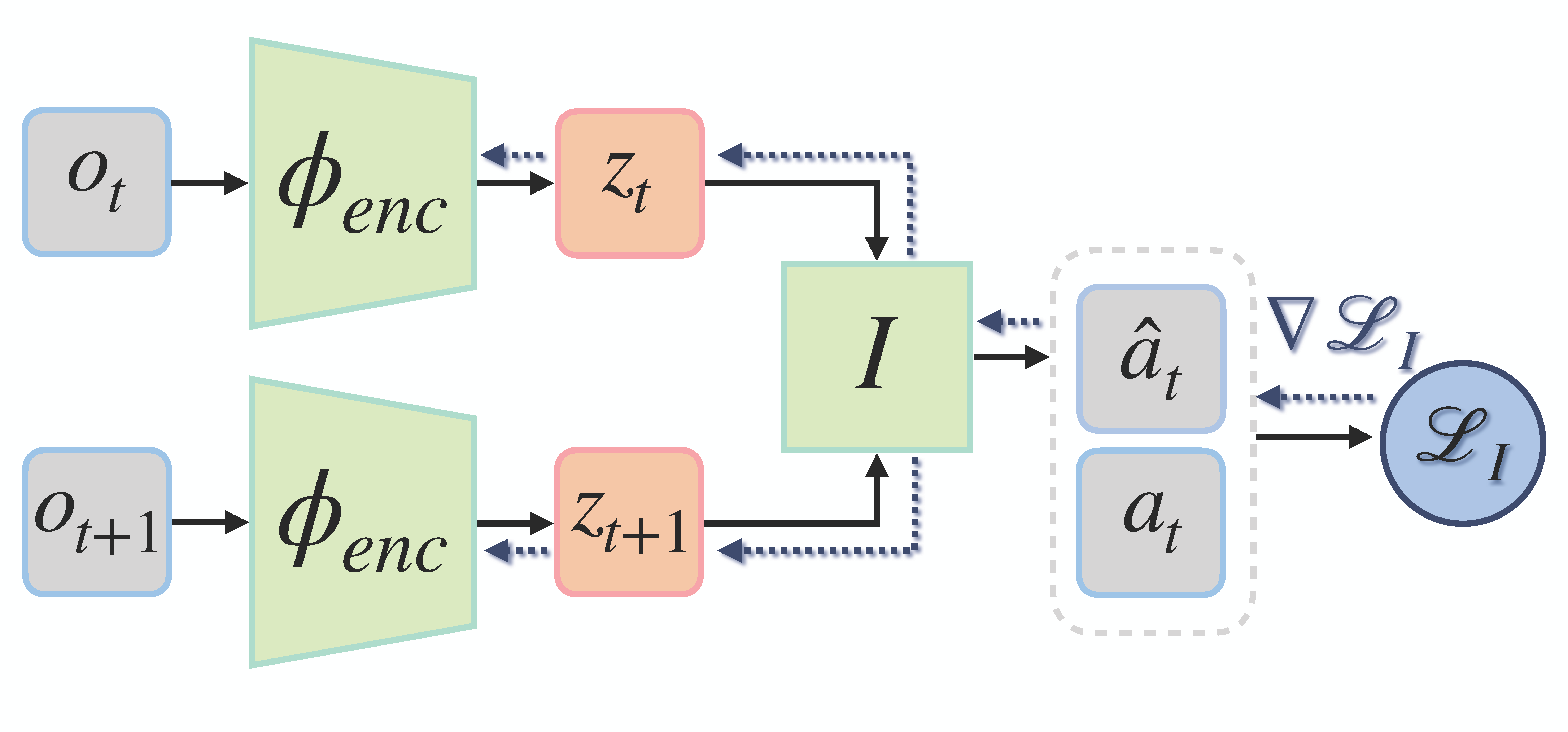
Figure 10: Latent inverse model. The solid line represents the forward pass of the data through the networks, while the dashed lines the gradient flow.

In DRL, the action space can be either continuous or discrete. Therefore, the loss function for training the latent inverse model can be either a MSE loss (see Equation (15) for continuous action spaces:

$$\begin{split}\min_{\bm{\theta}_{\text{enc}},\bm{\theta}_{I}}&\ \ \ \ \mathcal{L}_{{I}}(\bm{\theta}_{\text{enc}},\bm{\theta}_{I})\\ \mathcal{L}_{{I}}(\bm{\theta}_{\text{enc}},\bm{\theta}_{I})&=\mathbb{E}_{\bm{o}_{t},\bm{a}_{t},\bm{o}_{t+1}\sim\mathcal{D}}[\mid\mid\bm{a}_{t}-\hat{\bm{a}}_{t}\mid\mid^{2}]\\ &=\mathbb{E}_{\bm{o}_{t},\bm{a}_{t},\bm{o}_{t+1}\sim\mathcal{D}}[\mid\mid\bm{a}_{t}-I(\bm{z}_{t},\bm{z}_{t+1};\bm{\theta}_{I})\mid\mid^{2}]\\ &=\mathbb{E}_{\bm{o}_{t},\bm{a}_{t},\bm{o}_{t+1}\sim\mathcal{D}}[\mid\mid\bm{a}_{t}-I(\phi_{\text{enc}}(\bm{o}_{t};\bm{\theta}_{\text{enc}}),\phi_{\text{enc}}(\bm{o}_{t+1};\bm{\theta}_{\text{enc}});\bm{\theta}_{I})\mid\mid^{2}]\,,\end{split}$$ (15)

or, for discrete action spaces, the cross-entropy loss used for solving a multi-class classification problem (see Equation (16)).

$$\begin{split}\min_{\bm{\theta}_{\text{enc}},\bm{\theta}_{I}}&\ \ \ \ \mathcal{L}_{{I}}(\bm{\theta}_{\text{enc}},\bm{\theta}_{I})\\ \mathcal{L}_{{I}}(\bm{\theta}_{\text{enc}},\bm{\theta}_{I})&=\mathbb{E}_{\bm{o}_{t},\bm{a}_{t},\bm{o}_{t+1}\sim\mathcal{D}}[-\sum_{i\in|\mathcal{A}|}a^{i}_{t}\,\log\hat{\bm{a}}_{t}]\\ &=\mathbb{E}_{\bm{o}_{t},\bm{a}_{t},\bm{o}_{t+1}\sim\mathcal{D}}[-\sum_{i\in|\mathcal{A}|}a^{i}_{t}\,\log I(\bm{z}_{t},\bm{z}_{t+1};\bm{\theta}_{I})]\,,\end{split}$$ (16)

where $\bm{a}_{t}$ is the action label, $a^{i}_{t}$ the $i^{th}$-component of the action $\bm{a}_{t}$, and $\hat{\bm{a}}_{t}$ is a probability value obtained by applying a softmax activation at the output of the latent inverse model $I$. The softmax activation is only used in the context of discrete action spaces and in combination with the cross-entropy loss. In the continuous action spaces, the output of the inverse model is either bounded, e.g. by a tanh, or unbounded, e.g. via a linear activation.

Latent forward, inverse, and reward models are often used and optimized jointly for improving the quality of the learned state representations as shown in Equation (17).

$$\begin{split}\min_{\bm{\theta}_{\text{enc}},\bm{\theta}_{T},\bm{\theta}_{I},\bm{\theta}_{R}}\ \ \ \ &\omega_{{T}}\mathcal{L}_{{T}}(\bm{\theta}_{\text{enc}},\bm{\theta}_{T})+\omega_{{I}}\mathcal{L}_{{I}}(\bm{\theta}_{\text{enc}},\bm{\theta}_{I})+\omega_{{R}}\mathcal{L}_{{R}}(\bm{\theta}_{\text{enc}},\bm{\theta}_{R})\,,\end{split}$$ (17)

where $\omega_{{T}}$, $\omega_{{I}}$ and $\omega_{{R}}$ are three scalar factors for scaling the contribution of each loss.

Similar loss functions for learning state representations for DRL are used, for example, in [34, 35, 36, 37].

A fundamental concept in RL is the notion of MDP homomorphism [38]. The idea is to exploit the symmetries of the problem to transform a high-dimensional (in states and actions) and potentially complex MDP $\mathcal{M}$ into a low-dimensional MDP $\bar{\mathcal{M}}$ that is easier to solve. Moreover, because we learn a homomorphism between two MDPs, this framework guarantees that the optimal policy learned for the low-dimensional MDP $\bar{\mathcal{M}}$ can be lifted while maintaining its optimality to the original high-dimensional MDP $\mathcal{M}$. This statement implies that once we learn the optimal policy for $\bar{\mathcal{M}}$, this policy is the optimal policy for $\mathcal{M}$. Below we provide the formal definitions:

Definition 4.

Stochastic MDP Homomorphism: A stochastic MDP homomorphism $h$ from an MDP $\mathcal{M}=\langle\mathcal{S},\mathcal{A},T,R\rangle$ to an MDP $\mathcal{\bar{M}}=\langle\mathcal{\bar{S}},\mathcal{\bar{A}},\bar{T},\bar{R}\rangle$ is a tuple $\langle f,g_{\bm{s}}\rangle$, with:

• $f:\mathcal{S}\longrightarrow\mathcal{\bar{S}}$

• $g_{\bm{s}}:\mathcal{A}\longrightarrow\mathcal{\bar{A}}$

such that the following identities hold:

$$\forall_{\bm{s},\bm{s}^{\prime}\in\mathcal{S},\bm{a}\in\mathcal{A}}\ \ \ \bar{T}(f(\bm{s}^{\prime})|f(\bm{s}),g_{\bm{s}}(\bm{a}))=\sum_{\bm{s}^{\prime\prime}\in{[\bm{s}^{\prime}]_{f}}}\text{T}(\bm{s}^{\prime\prime}|\bm{s},a)$$ (18)

$$\forall_{\bm{s},\bm{a}\in\mathcal{A}}\ \ \ \bar{R}(f(\bm{s}),g_{\bm{s}}(\bm{a}))=R(\bm{s},\bm{a})\,,$$ (19)

where $[\bm{s}^{\prime}]_{f}$ is the equivalence class of $\bm{s}^{\prime}$ under $f$.

Definition 5.

Deterministic MDP Homomorphism: A deterministic MDP homomorphism $h$ from an MDP $\mathcal{M}=\langle\mathcal{S},\mathcal{A},T,R\rangle$ to an MDP $\mathcal{\bar{M}}=\langle\mathcal{\bar{S}},\mathcal{\bar{A}},\bar{\text{T}},\bar{\text{R}}\rangle$ is a tuple $\langle f,g_{\bm{s}}\rangle$, with:

• $f:\mathcal{S}\longrightarrow\mathcal{\bar{S}}$

• $g_{\bm{s}}:\mathcal{A}\longrightarrow\mathcal{\bar{A}}$

such that the following identities hold:

$$\forall_{\bm{s},\bm{s}^{\prime}\in\mathcal{S},\bm{a}\in\mathcal{A}}\ \ \ \text{T}(\bm{s},\bm{a})=\bm{s}^{\prime}\Longrightarrow\bar{\text{T}}(f(\bm{s}),g_{\bm{s}}(\bm{a}))=f(\bm{s}^{\prime})$$ (20)

$$\forall_{\bm{s}\in\mathcal{S},\bm{a}\in\mathcal{A}}\ \ \ \bar{\text{R}}(f(\bm{s}),g_{\bm{s}}(\bm{a}))=\text{R}(\bm{s},\bm{a})$$ (21)

If Equation (18) and (19) are satisfied, the (stochastic) policy $\bar{\pi}_{\bar{\mathcal{M}}}$ of the homomorphic image $\bar{\mathcal{M}}$ can be lifted to the original MDP $\mathcal{M}$, and we denote it as $\pi_{\mathcal{M}}$, such that for any $\bm{a}\in g_{\bm{s}}^{-1}$:

$$\pi_{\mathcal{M}}(\bm{a}|\bm{s})=\bar{\pi}_{\bar{\mathcal{M}}}(\bar{\bm{a}}|f(\bm{s}))/\mid g_{\bm{s}}^{-1}(\bar{\bm{a}})\mid\,,$$ (22)

where for any $\bm{s}$, $g_{\bm{s}}^{-1}(\bar{\bm{a}})$ denotes the set of actions that have the same image $\bar{\bm{a}}\in\mathcal{\bar{A}}$ under $g_{\bm{s}}$, and $\bar{\bm{a}}=g_{\bm{s}}(\bar{a})$.

In the context of SRL, it is possible to leverage the MDP homomorphism metric to learn the state representation. The MDP homomorphism metric makes use of an encoder $\phi_{\text{enc}}$ mapping observations to latent states, a transition $\bar{T}$, a reward model $\bar{R}$ to enforce the relation in Equation (20) and (21), and two additional models, namely $f:\mathcal{Z}\rightarrow\mathcal{\bar{Z}}$ and $g_{\bm{z}}:\mathcal{Z}\times\mathcal{A}\rightarrow\mathcal{\bar{A}}$ learning (latent) states and states-actions symmetries. The advantage of the MDP homomorphism metric is that, when minimized, i.e. $\mathcal{L}_{\bar{T}}\rightarrow 0$ and $\mathcal{L}_{\bar{R}}\rightarrow 0$, we obtain a MDP homomorphism exploiting the symmetries of the problem. The policy learned using this representation is guaranteed optimal for the original MDP too. Moreover, the latent state space is guaranteed to be Markovian. In Figure 11, the commutative diagram representing the MDP homomorphism is shown.

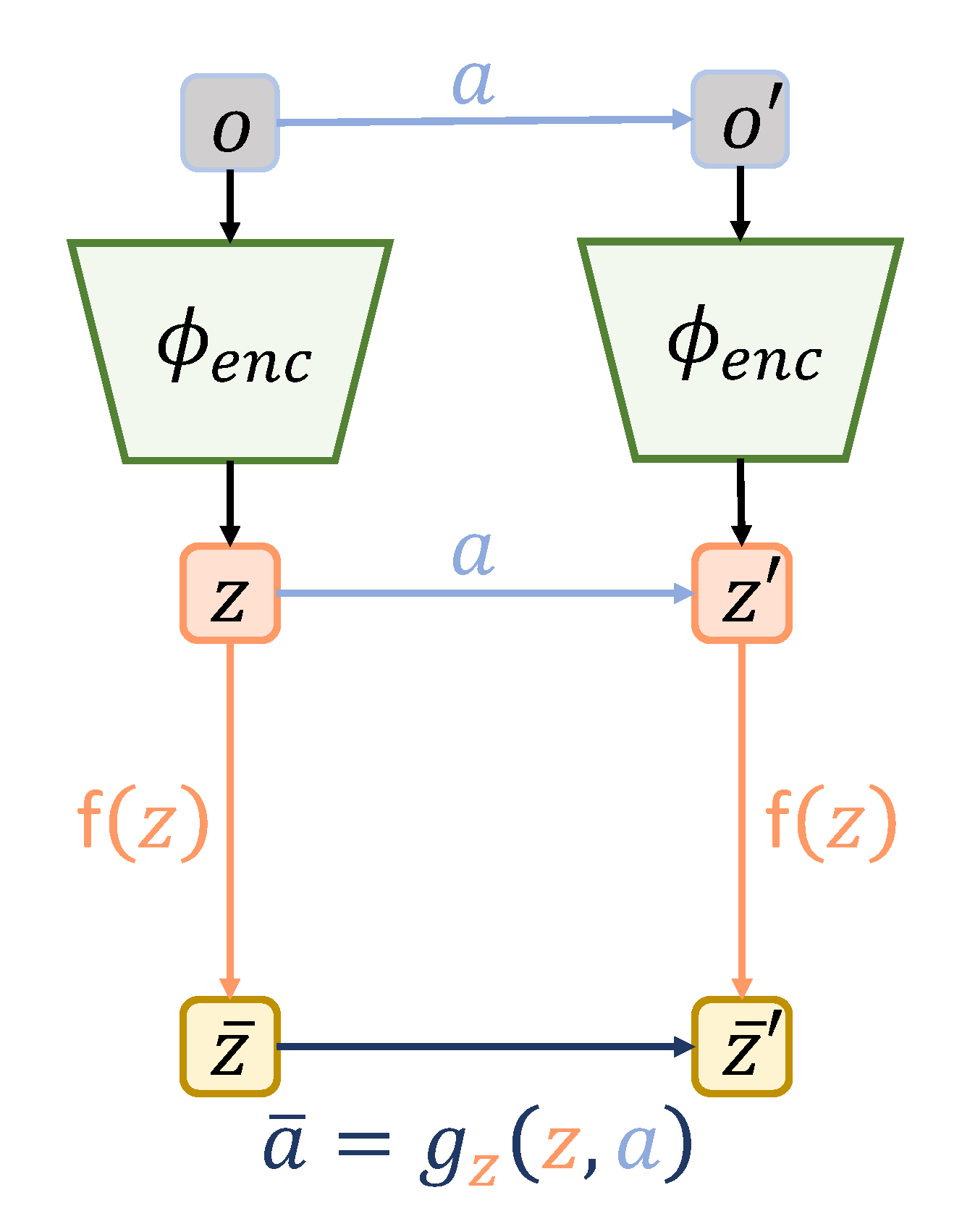
Figure 11: Commutative diagram. Encoding the observation $\bm{o}$ in $\bm{z}$ via the encoder $\phi_{\text{enc}}$ and applying action $a$ is equivalent to abstracting $\bm{z}$ via $f$ and transitioning via $\bar{\bm{a}}$.

However, learning forward and reward models is difficult for complex applications. The losses rarely converge globally and precisely to zero, and in most cases, we end up with an approximate MDP homomorphism [39].

A closely-related concept to the MDP homomorphism that can be used for learning compact representations is the bisimulation metric [40, 41]. For large MDP, we can think of partitioning the state space into sets of states with equivalent behavior, with the equivalence defined by the bisimulation relation $E\subseteq\mathcal{S}\times\mathcal{S}$:

$$\bm{s}^{\prime}E\bm{s}^{\prime\prime}\iff\forall\bm{a}\ R(\bm{s}^{\prime},\bm{a})=R(\bm{s}^{\prime\prime},\bm{a})\ \ \ \land\ \ \ \forall X\in\mathcal{S}/E\ p(X^{\prime}|\bm{s}^{\prime},\bm{a})=p(X|\bm{s}^{\prime\prime},\bm{a})$$ (23)

where $\mathcal{S}/E$ is the partition of $\mathcal{S}$ into $E$-equivalent subset of states. The bisimulation metric is the union of all the bisimulation relations. From (23) follows that two states are bisimilar if they have the same transition and reward and, consequently, the same value function. However, the bisimulation metric is difficult to satisfy completely and is not robust to small changes in the transition probabilities and rewards.

A lax bisimulation metric is introduced in [42] to exploit symmetries of the environment by relaxing the equality of the actions in the bisimulation metric in Equation (23). We can define the lax bisimulation relation $B$ as:

$$\bm{s}^{\prime}B\bm{s}^{\prime\prime}\iff\forall\bm{a}\ \exists\bm{b}\text{ such that }R(\bm{s}^{\prime},\bm{a})=R(\bm{s}^{\prime\prime},\bm{b})\ \ \ \land\ \ \ \forall X\in S/B\ p(X|\bm{s}^{\prime},\bm{a})=p(X|\bm{s}^{\prime\prime},\bm{b})$$ (24)

Again, the lax bisimulation metric is the union of the lax bisimulation relations. It is easy to see that the lax bisimulation metric is equivalent to the MDP homomorphism metric[42].

An example of a (deep) bisimulation metric in SRL is introduced in [43], where a state representation is learned such that the $L_{1}$ distances correspond to bisimulation metrics. The encoder $\phi_{\text{enc}}$ is by minimizing:

$$\begin{split}\min_{\bm{\theta}_{\text{enc}}}&\ \ \ \ \mathcal{L}_{\text{bm}}(\bm{\theta}_{\text{enc}})\\ \mathcal{L}_{\text{bm}}(\bm{\theta}_{\text{enc}})&=\mathbb{E}_{\bm{o},\bm{a},r,\bm{o}^{\prime}\sim\mathcal{D}}[(||\bm{z}_{t_{1}}-\bm{z}_{t_{2}}||_{1}-||\hat{r}_{t_{1}}-\hat{r}_{t_{2}}||_{1}-\gamma W_{2}(T(\bm{z}_{t_{1}+1}|\tilde{\bm{z}}_{t_{1}},\bm{a}_{t_{1}}),T(\bm{z}_{t_{2}+1}|\tilde{\bm{z}}_{t_{2}},\bm{a}_{t_{2}})))^{2}]\\ \end{split}$$ (25)

where $\bm{z}_{t_{1}}=\phi_{\text{enc}}(\bm{o}_{t_{1}})$, $\bm{z}_{t_{2}}=\phi_{\text{enc}}(\bm{o}_{t_{2}})$, $\tilde{z}$ indicates the stop of the gradients such that they do no propagate through the encoder, $\gamma$ is a scaling factor, and $W_{2}$ is the 2-Wasserstein metric. It is worth noticing that transition and reward models are used to compute the bisimulation loss in Equation (LABEL:eq:bisimulation_loss). However, these models are not updated jointly with the encoder, but in alternating fashion accordinhly to Equation $\eqref{eq:forward_model_loss}$ and (14).

3.2.4 Priors

When the underlying MDP model is a dynamic system fully or partially governed by the laws of physics, such as in robotics, we can encode such prior physical knowledge in the form of loss functions and use them to training of the encoder $\phi_{\text{enc}}$ such that the latent states evolve accordingly to these laws. For example, consider a mobile robot navigating based on onboard sensory readings; the underlying actual state space has specific properties dictated by the laws of physics. Therefore, we can shape the loss functions using the physical laws to learn smooth and coherent state representations.

These loss functions, called robotics priors [28], do not rely on any auxiliary morel, e.g. forward or reward model, and can be used to directly train the encoder, as shown in Figure 12.

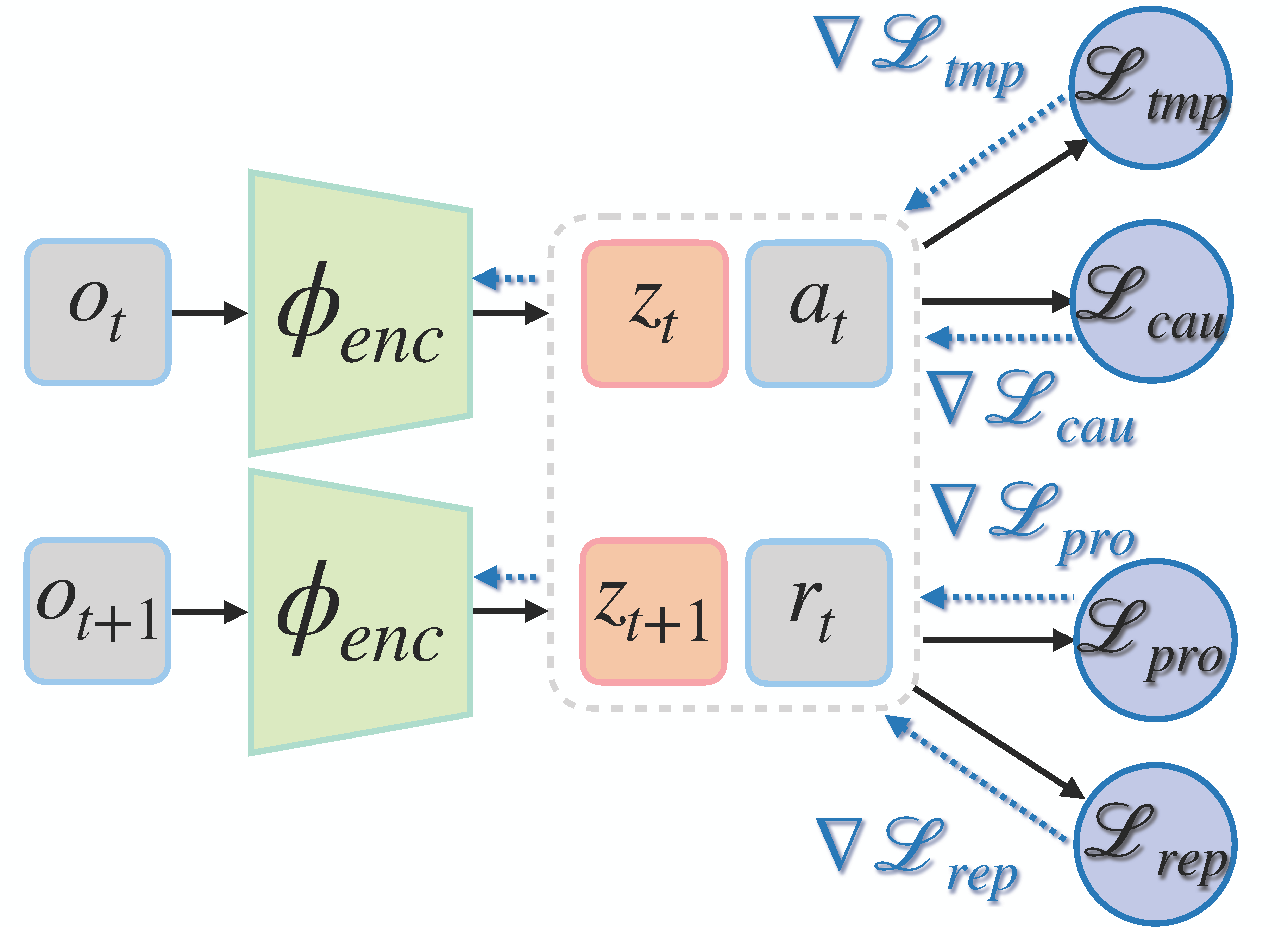
Figure 12: Robotics Priors. The solid line represents the forward pass of the data through the networks, while the dash lines the gradient flow.

An example of robotics prior is the temporal coherence loss introduced in [28] and shown in Equation (26).

$$\begin{split}\min_{\bm{\theta}_{\text{enc}}}&\ \ \ \ \mathcal{L}_{\text{tmp}}(\bm{\theta}_{\text{enc}})\\ \mathcal{L}_{\text{tmp}}(\bm{\theta}_{\text{enc}})&=\mathbb{E}_{\bm{o},\bm{o}^{\prime}\sim\mathcal{D}}[||\Delta\bm{z}_{t}||^{2}]\\ &=\mathbb{E}_{\bm{o},\bm{o}^{\prime}\sim\mathcal{D}}[||\bm{z}_{t+1}-\bm{z}_{t}||^{2}]\end{split}$$ (26)

The temporal coherence loss enforces smooth and small changes in the learned state space between pairs of consecutive latent states. The prior knowledge enforced by this loss function is the assumption that the actual state space is smooth and continuous. This property of the state space is valid for environment obeying physical laws, e.g. robotics.

The temporal coherence prior alone is insufficient for learning an informative state representation. The global minimum of such loss function is reached when mapping each latent state to the zero vector. Therefore, to prevent the learning of the trivial mapping, the causality loss is introduced. This prior, see Equation (27), utilises pairs of latent states, collected at different time instants $t_{1}$ and $t_{2}$ when the same actions $\bm{a}_{t_{1}},\bm{a}_{t_{2}}$ is taken from such states, but the rewards received are different $r_{t_{1}},r_{t_{2}}$, and it is minimised when the two states predictions are pushed apart in the latent space.

$$\begin{split}\min_{\bm{\theta}_{\text{enc}}}&\ \ \ \ \mathcal{L}_{\text{cau}}(\bm{\theta}_{\text{enc}})\\ \mathcal{L}_{\text{cau}}(\bm{\theta}_{\text{enc}})&=\mathbb{E}_{\bm{o},\bm{a},r,\bm{o}^{\prime}\sim\mathcal{D}}[e^{-||\bm{z}_{t_{1}}-\bm{z}_{t_{2}}||^{2}}|\bm{a}_{t_{1}}=\bm{a}_{t_{2}},r_{t_{1}}\neq r_{t_{2}}]\end{split}$$ (27)

When the same actions $\bm{a}_{t_{1}},\bm{a}_{t_{2}}$ are applied in different states, we want our state variations $\Delta\bm{z}_{t_{1}}=\bm{z}_{t_{1}+1}-\bm{z}_{t_{1}}$ and $\Delta\bm{z}_{t_{2}}=\bm{z}_{t_{2}+1}-\bm{z}_{t_{2}}$ to be similar in magnitude. This prior is encoded by the proportionality loss and shown in Equation (28).

$$\begin{split}\min_{\bm{\theta}_{\text{enc}}}&\ \ \ \ \mathcal{L}_{\text{pro}}(\bm{\theta}_{\text{enc}})\\ \mathcal{L}_{\text{pro}}(\bm{\theta}_{\text{enc}})&=\mathbb{E}_{\bm{o},\bm{a},\bm{o}^{\prime}\sim\mathcal{D}}[(||\Delta\bm{z}_{t_{1}}||-||\Delta\bm{z}_{t_{2}}|)^{2}|\bm{a}_{t_{1}}=\bm{a}_{t_{2}}]\end{split}$$ (28)

Another example is the repeatability loss, in Equation (LABEL:eq:repeatexample), enforcing that state changes produced by the same action to be equal in magnitude and direction.

$$\begin{split}\min_{\bm{\theta}_{\text{enc}}}&\ \ \ \ \mathcal{L}_{\text{rep}}(\bm{\theta}_{\text{enc}})\\ \mathcal{L}_{\text{rep}}(\bm{\theta}_{\text{enc}})&=\mathbb{E}_{\bm{o},\bm{a},r,\bm{o}^{\prime}\sim\mathcal{D}}[e^{-||\bm{z}_{t_{1}}-\bm{z}_{t_{2}}||^{2}}||\Delta\bm{z}_{t_{2}}-\Delta\bm{z}_{t_{1}}||^{2}|\bm{a}_{t_{1}}=\bm{a}_{t_{2}}]\\ \end{split}$$ (29)

Eventually, to obtain an informative and coherent state representation, the encoder $\phi_{\text{enc}}$ is then usually trained by jointly minimizing the sum of multiple robotics priors losses [28], as shown in Equation (30).

$$\begin{split}\min_{\bm{\theta}_{\text{enc}}}\ \ \ \ &\omega_{\text{t}}\mathcal{L}_{\text{tem}}(\bm{\theta}_{\text{enc}})+\omega_{\text{c}}\mathcal{L}_{\text{cau}}(\bm{\theta}_{\text{enc}})+\omega_{\text{p}}\mathcal{L}_{\text{pro}}(\bm{\theta}_{\text{enc}})+\omega_{\text{r}}\mathcal{L}_{\text{rep}}(\bm{\theta}_{\text{enc}})\\ \end{split}$$ (30)

where $\omega_{\text{t}}$, $\omega_{\text{c}}$, $\omega_{\text{p}}$, and $\omega_{\text{r}}$ are scaling factors for scaling the contribution of each loss.

While allowing efficient learning of state representation for simple robotics tasks, the robotics priors struggle in generalizing, e.g. in the presence of domain randomization, and robustness when the observations include visual distractors [45].

3.2.5 Contrastive Learning

Contrastive learning [29] is an unsupervised approach for learning data representations by only relying on similarities and dissimilarities of data pairs. Contrastive learning has achieved impressive results in DL, and in the most recent years, this paradigm has been used in unsupervised state representation learning more and more often. Nowadays, contrastive learning is a crucial element for sample-efficient DRL [46].

The critical ingredient of contrastive learning is contrastive loss. Contrastive losses act on pairs of embeddings, and through their minimization, they push apart negative pairs, i.e. data non-belonging to the same class or non-consecutive observations in the context of DRL. Additionally, contrastive losses prevent the collapsing of the representations to trivial embeddings when no labelled data are available. However, contrastive losses must always be combined with another loss function to effectively improve DRL algorithms’ performance. Many contrastive losses have been proposed in the DL literature, but here we focus on the most widely used in DRL: (i) InfoNCE, (ii) hinge, and (iii) causality loss.

Contrastive Predictive Coding (CPC) was introduced in [47] for unsupervised learning of representations of future observations given the past ones. CPC has been employed in unsupervised learning of visual representation, supervised learning [48], data-efficient supervised learning [49], and DRL for sample-efficient learning of state representations [46, 50, 51]. CPC employs the so-called InfoNCE loss (Equation (31)). Optimizing InfoNCE allows the neural networks to learn (future) representations from negative samples.

Given a set $X$ of $N$ random samples containing one positive samples from $p(\bm{x}_{t}|\bm{c}_{t})$, where $\bm{c}_{t}=h(\bm{z}_{t},\cdot\bm{z}_{t-r})$ is the context vector summarizing time information from the latent states and $h$ is an autoregressive model, and $N-1$ negative samples from the proposal distribution $p(\bm{x}_{t+k})$, we optimize:

$$\mathcal{L}_{\text{InfoNCE}}=-\mathbb{E}_{X}\Big{[}\log\frac{f_{k}(\bm{x}_{t+k},\bm{c}_{t})}{\sum_{x_{j}\in X}f_{k}(\bm{x}_{j},\bm{c}_{t})}\Big{]}$$ (31)

where $f_{k}(\bm{x}_{t+k},\bm{c}_{t})\propto\frac{p(\bm{x}_{t+k}|\bm{c}_{t})}{p(\bm{x}_{t+k})}$ is the density ratio preserving the mutual information between $\bm{x}_{t+k}$ and $\bm{c}_{t}$. In practice, $f_{k}(\bm{x}_{t+k},\bm{c}_{t})=\exp(\bm{z}_{t+k}^{T}W_{k}\bm{c}_{t})$ with $W_{k}$ a learnable linear transformation. The InfoNCE loss is categorical cross-entropy of classifying the positive samples correctly.

An adaptation of InfoNCE loss for SRL is proposed by [46], where the positive samples and context vectors are obtained by encoding the same observations $\bm{o}$ but with different augmentation techniques (e.g. different cropping) applied on them. In contrast, the negative examples are a set of encoded randomly-sampled observations.

Another example of contrastive loss for unsupervised learning of representation is the hinge loss [31, 33, 52].

$$\mathcal{L}_{\text{hinge}}(\phi_{\text{enc}})=\mathbb{E}_{\bm{o},\bm{o}^{\neg}\sim\mathcal{D}}[\max(0,\epsilon-d(\bm{z},\bm{z}^{\neg})]$$ (32)

where the distance $d(,)$ between two non-consecutive embeddings $\bm{z}$ and $\bm{z}^{\neg}$ and $\epsilon$ is a scaling parameter. The operator $\max(\cdot,\cdot)$ prevents the distance from growing indefinitely. The minimization of $\mathcal{L}_{\text{hinge}}$ pushes apart non-consecutive state pairs.

Another example is the causality loss introduced by [28] pushing apart pairs of state predictions when the same action is applied, but the reward received is different.

$$\mathcal{L}_{\text{cau}}=\mathbb{E}_{\bm{o},\bm{a},r,\bm{o}^{\neg}\sim\mathcal{D}}[e^{-||\bm{z}_{t_{1}}-\bm{z}_{t_{2}}||^{2}}|\bm{a}_{t_{1}}=\bm{a}_{t_{2}},r_{t_{1}}\neq r_{t_{2}}]$$ (33)

The causality loss can be generalized by removing the conditioning on action and rewards and used to push apart non-consecutive state predictions. This loss is used in [32].

$$\mathcal{L}_{\text{cau}}=\mathbb{E}_{\bm{o},\bm{o}^{\neg}\sim\mathcal{D}}[e^{-||\bm{z}_{t_{1}}-\bm{z}_{t_{2}}||^{2}}]$$ (34)

3.3 Summary

In the previous section, we introduced the four major categories of SRL methods. Methods from these categories are often combined to allow the learning of better state representations. We will discuss these advanced methods in Section Unsupervised Representation Learning in Deep Reinforcement Learning.

In Table 1, we relate the methods introduced in the previous sections to the properties of the learned state space (see Section Properties of the Learned State Representations). In particular, smoothness and low-dimensionality are naturally provided by neural networks and therefore are achieved by each method. However, obtaining simple and quasi-linear transitions between latent states or a Markovian latent state space $\mathcal{Z}$ is often hard in practice. The former property can be achieved by minimizing the distance between consecutive states and is related to the idea of temporal coherence loss (see Equation (26)). At the same time, the latter requires learning the reward and transition functions. A common trait of all methods is sufficient expressiveness, as they proved to be successful in the literature for providing a state representation that allows policy learning and solving various problems.

Table 1: Relation between the SRL methods and the desired properties of the latent space $\mathcal{Z}$ (described in Section Properties of the Learned State Representations). Each method is graded with yes/no (/), low (), medium (), or high ().

Method ($\downarrow$) - Property ($\rightarrow$)	Latent state space smoothness	Ability to reduce dimensionality	Complexity of the dependencies	Markovian	Temporal coherence	Expressiveness
Principal Component Analysis (PCA)
Autoencoders (AE)
Variational Autoencoders (VAE)
Forward Model (FW)
Reward Model (RW)
Inverse Model (IN)
MDP Homomorphism (MDPH) [33]
Bisimulation Metric (BM) [43]
Priors (PR) [53]
Contrastive Learning (CL)
Autoencoders with Forward Model (AEFW)
Autoencoders with Reward Model (AERW)
Autoencoders with Inverse Model (AEIN)
Forward Model with Contrastive Learning (FWCL))
Forward and Reward Model (FWRW)
Forward, Reward, and Inverse Model (FWRWIN)

To qualitatively evaluate the latent state space smoothness, we implemented the different methods described in Section Deep Learning for Learning State Representations and some combinations of them, as reported in Table 1. The experiments consist of learning a compact representation for a pendulum from high-dimensional observations (i.e. RGB images) without distractor, with fixed distractor, and with a randomly-positioned distractor. Examples of observations are shown in Figure 13. Details of the experiments and code implementation are provided in Implementation Details.

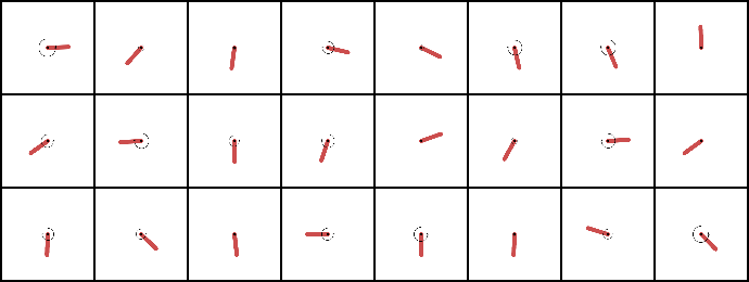
(a) No distractor.

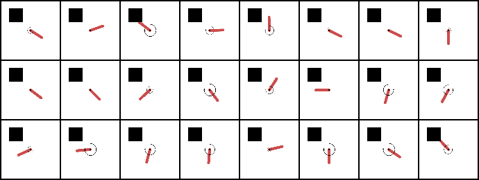
(b) Fixed distractor.

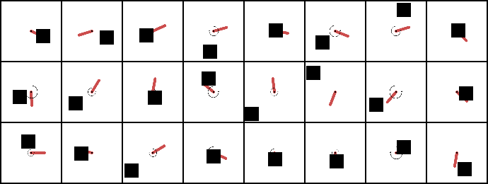
(c) Randomly-positioned distractor.

Figure 13: Different observation types.

The state representations learned with the different methods in Table 1 from distractor-free observations (see Figure 13(a)) are shown in Figure 14 and 15, where the color bar represents the true angle of the pendulum and it is used for assessing the smoothness of the latent state space. A smooth representation should be able to encode similar observations, i.e. observations captured with similar angles of the pendulum, close together in the latent space. The state representations learned from observations with fixed distractors (see Figure 13(b)) are shown in Figure 16 and 17. Eventually, the state representations learned from observations with randomly-positioned distractors (see Figure 13(c)) are shown in Figure 18 and 19.

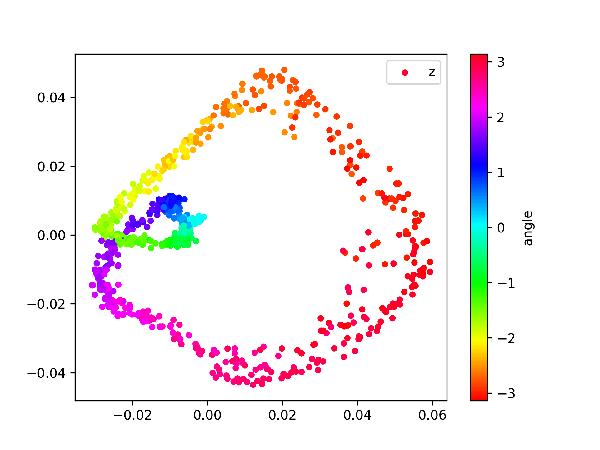
(a) PCA

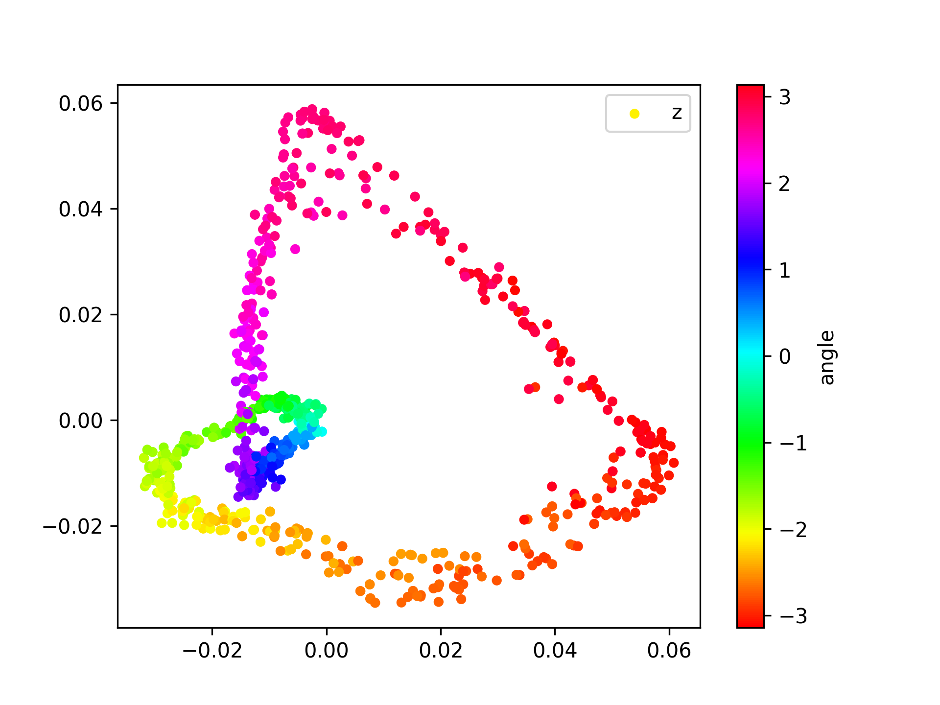
(b) AE

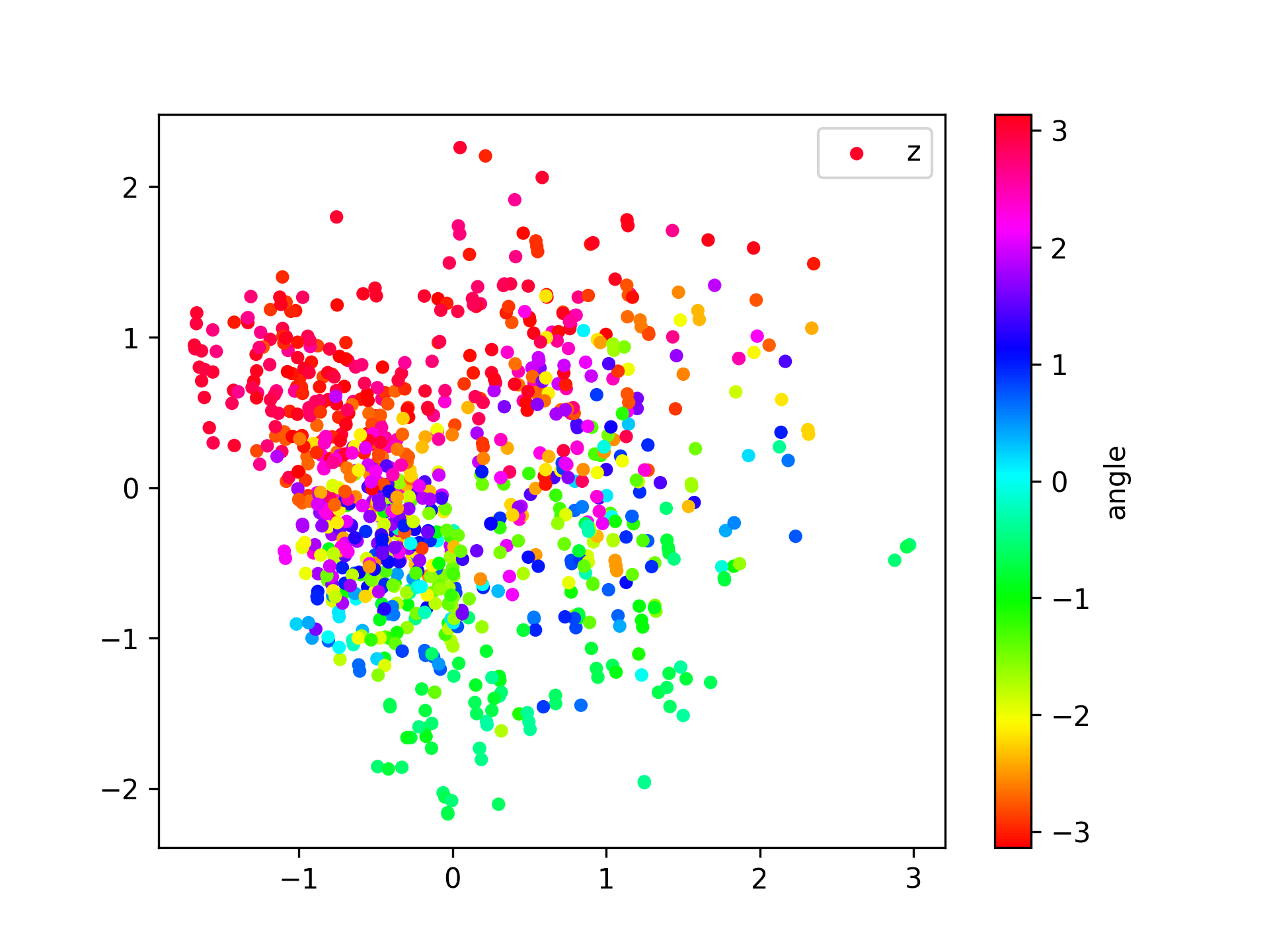
(c) VAE

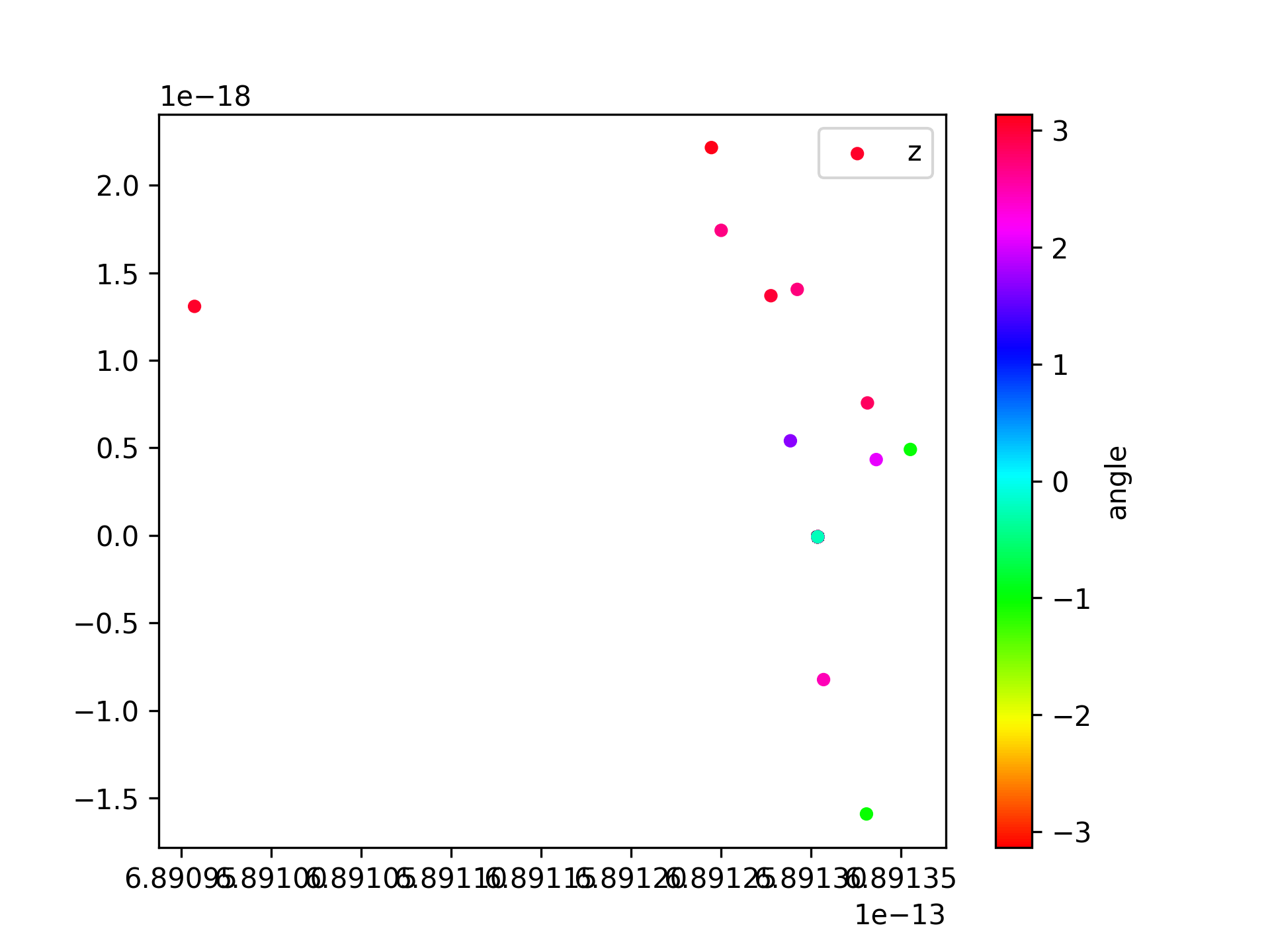
(d) FW

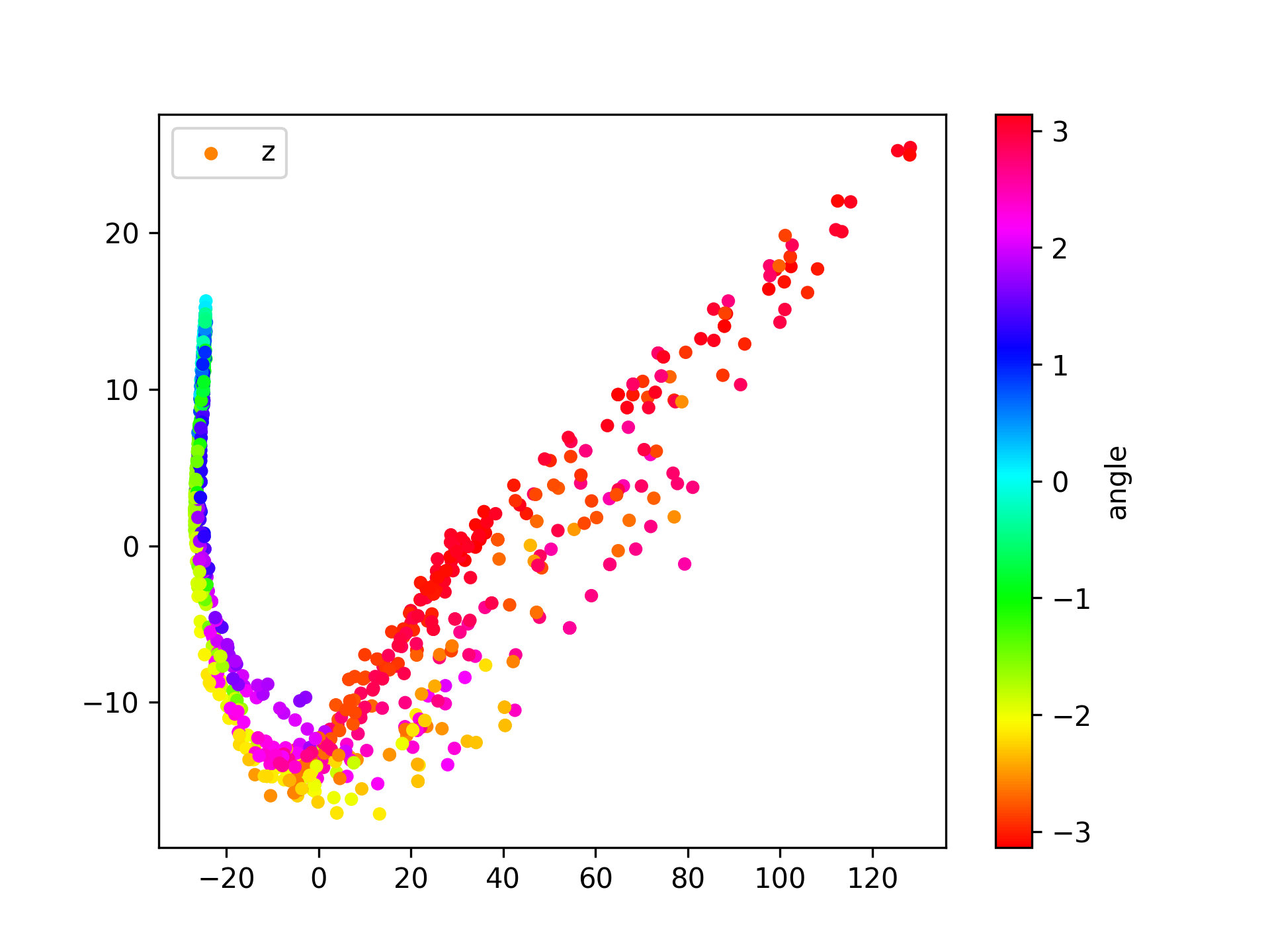
(e) RW

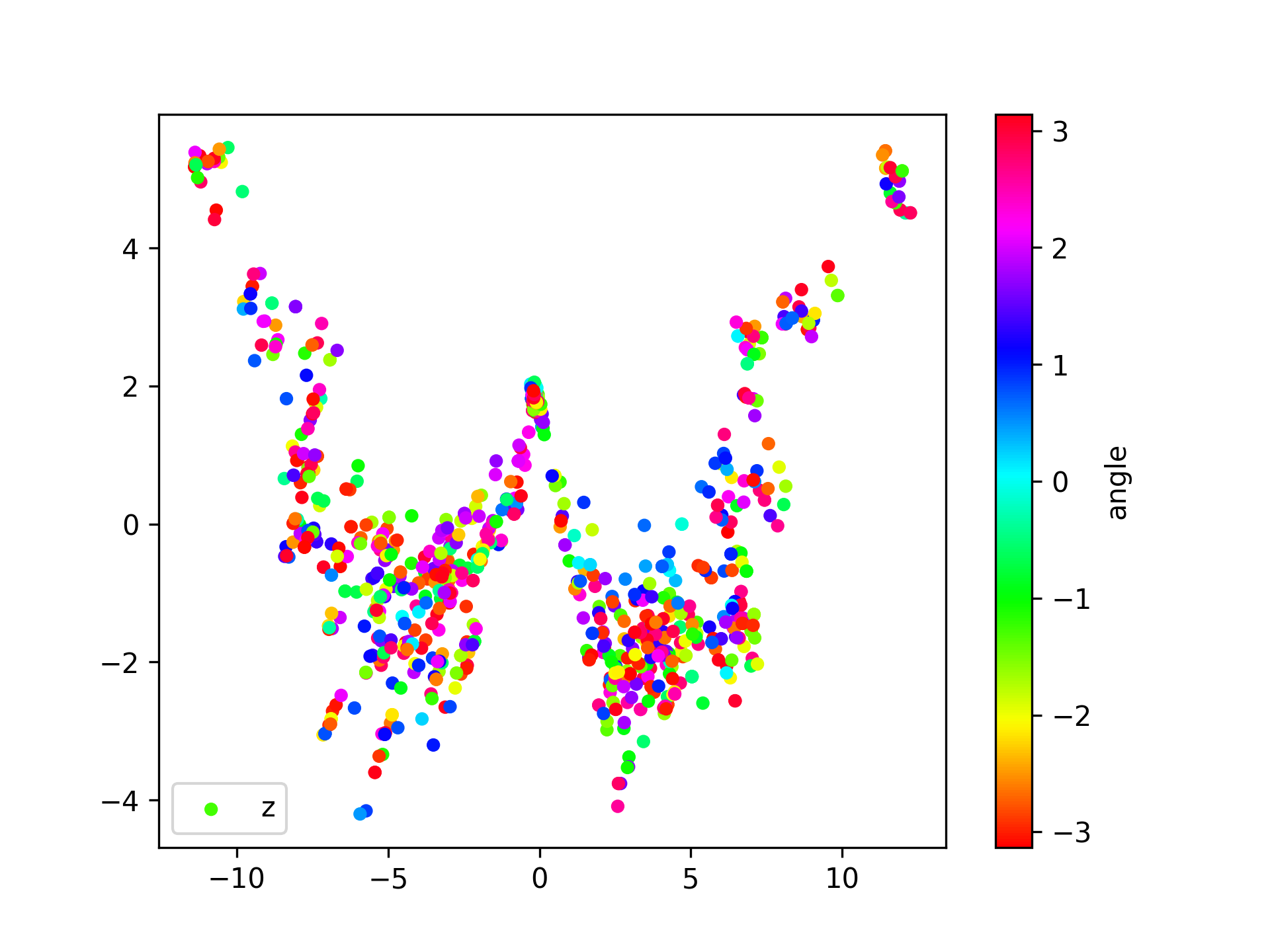
(f) IN

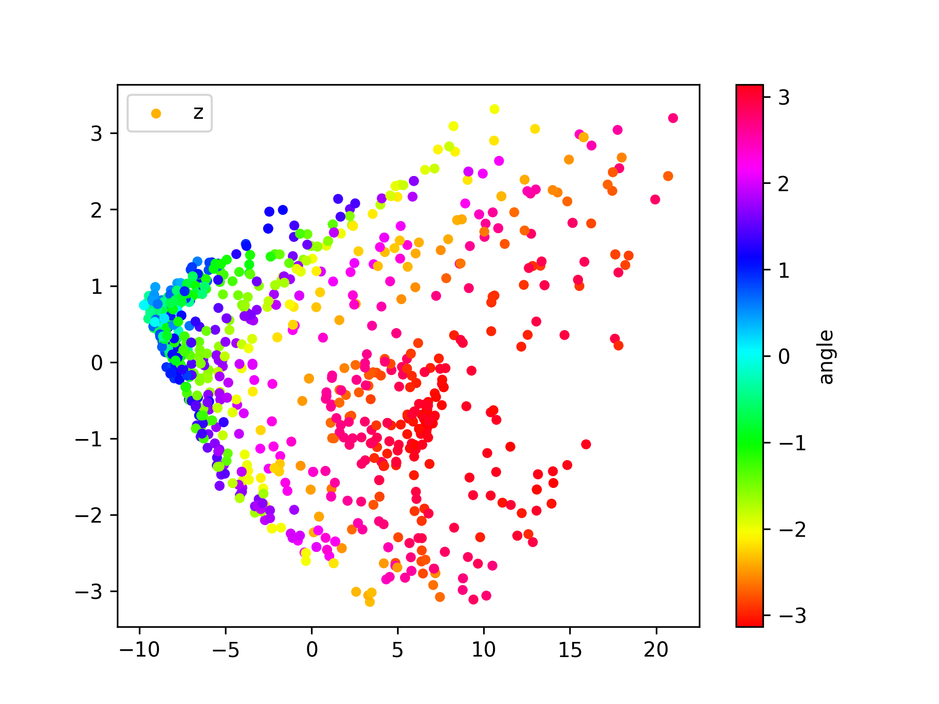
(g) MDPH

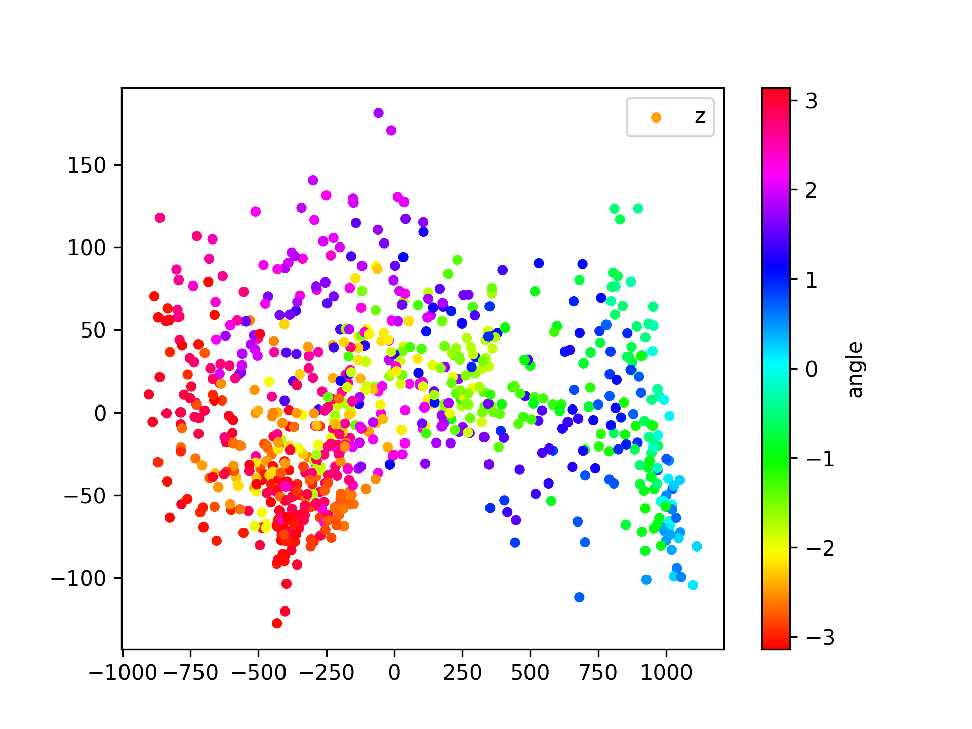
(h) BM

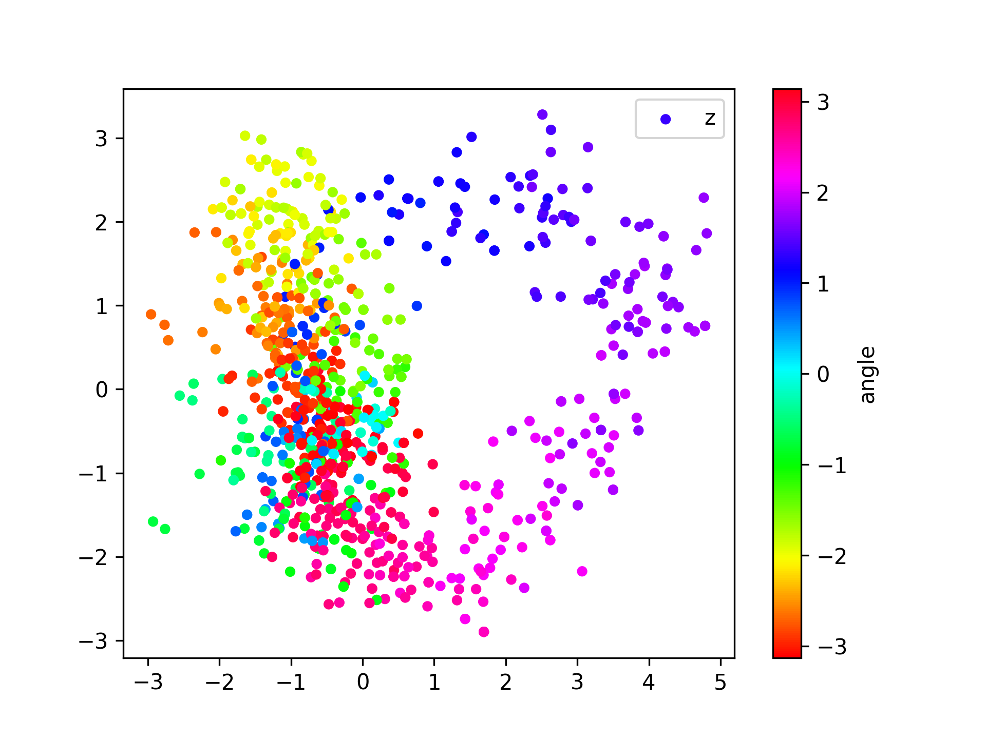
(i) PR

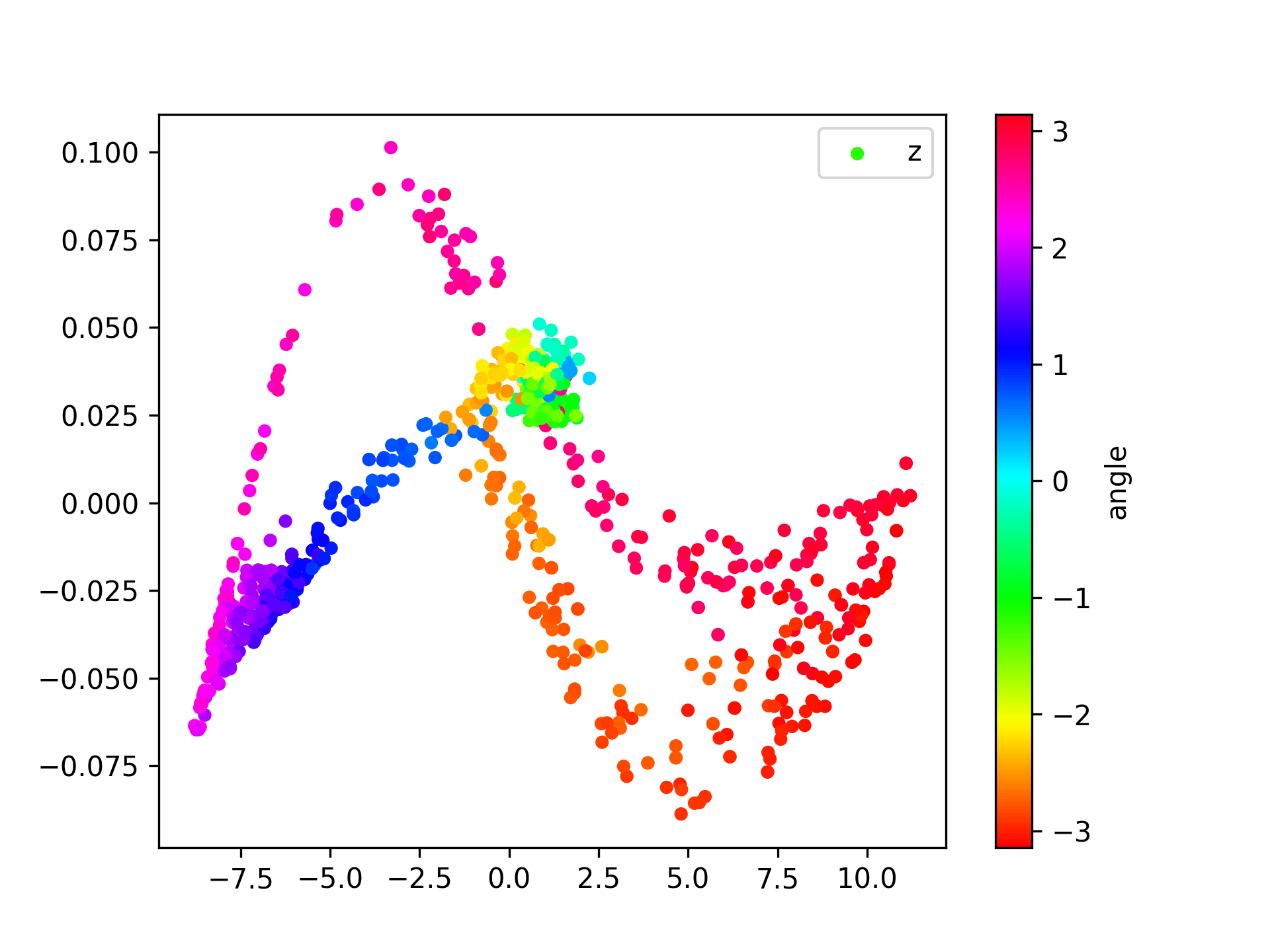
(j) CL

Figure 14: Learned state representations without distractors.

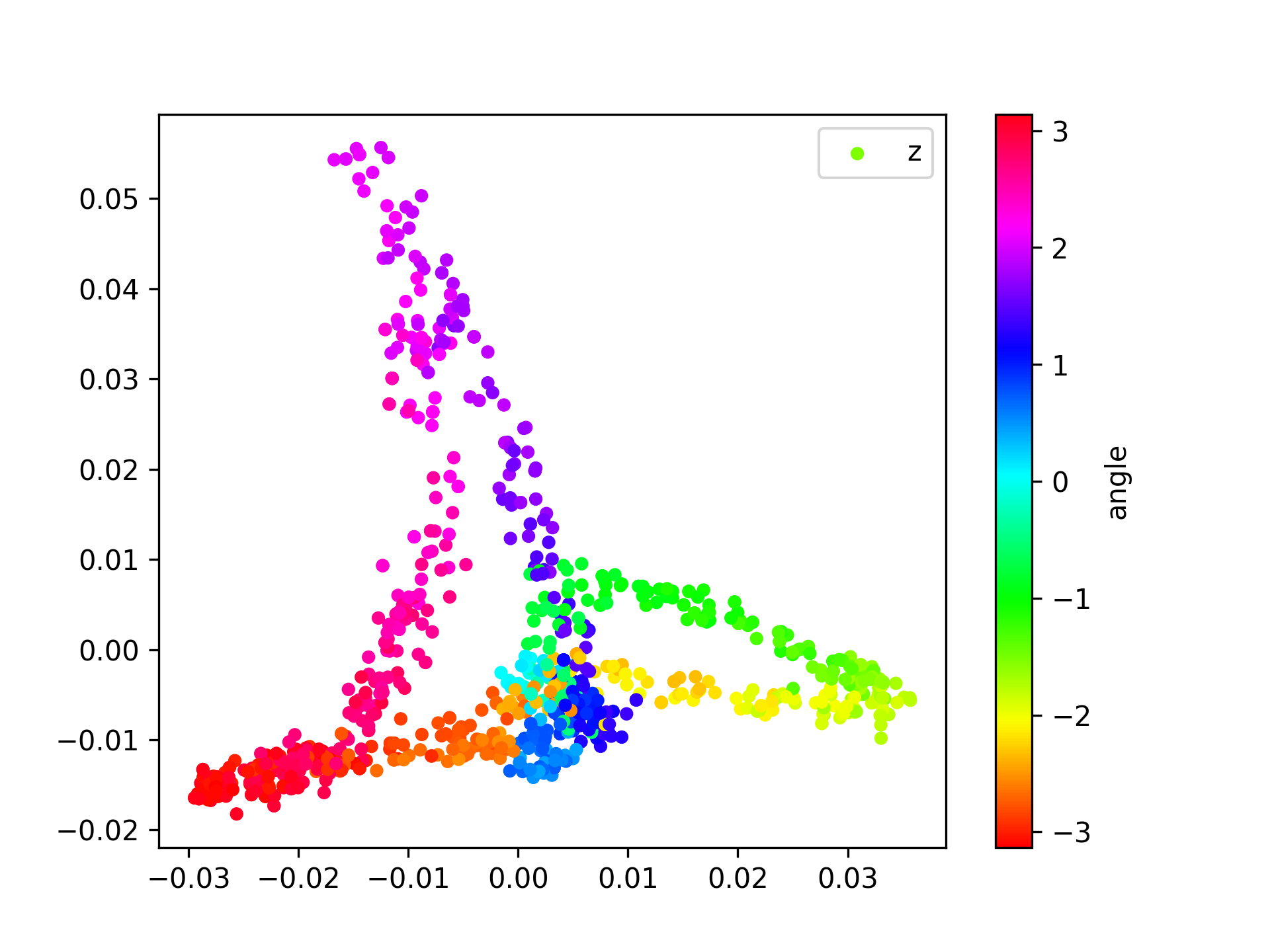
(a) AEFW

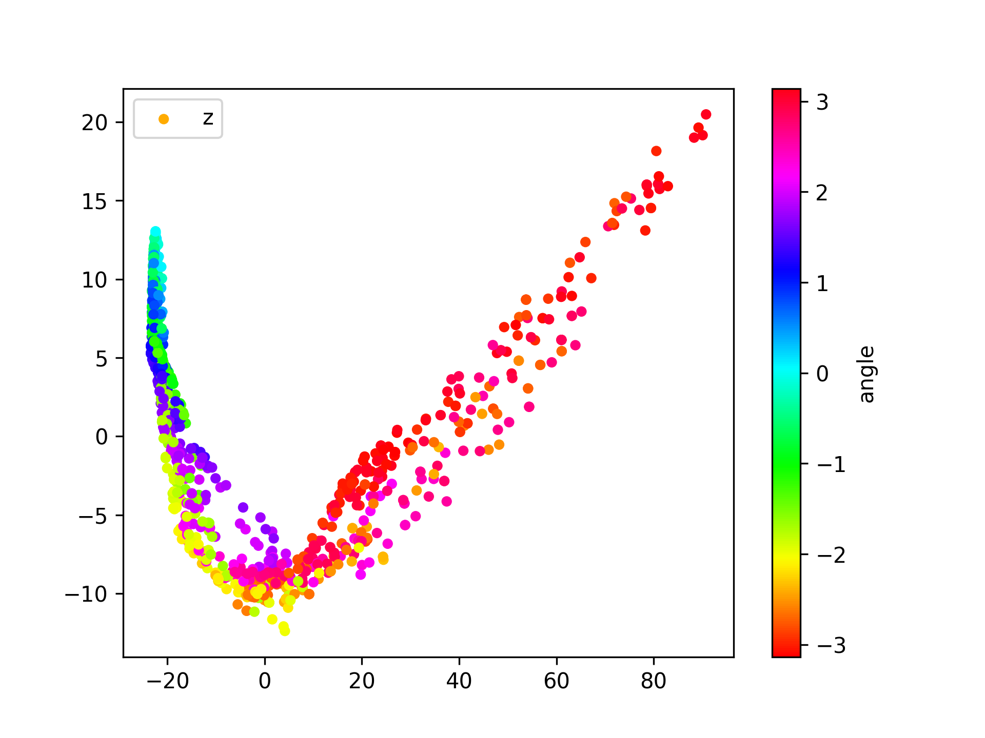
(b) AERW

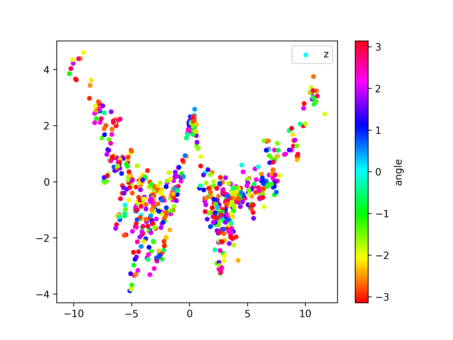
(c) AEIN

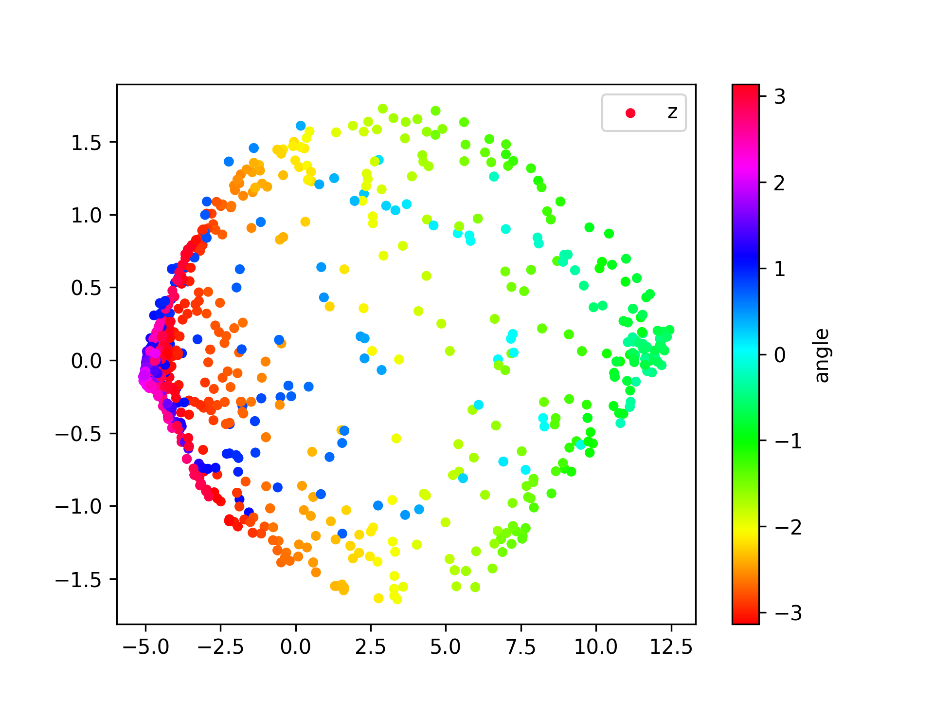
(d) FWCL

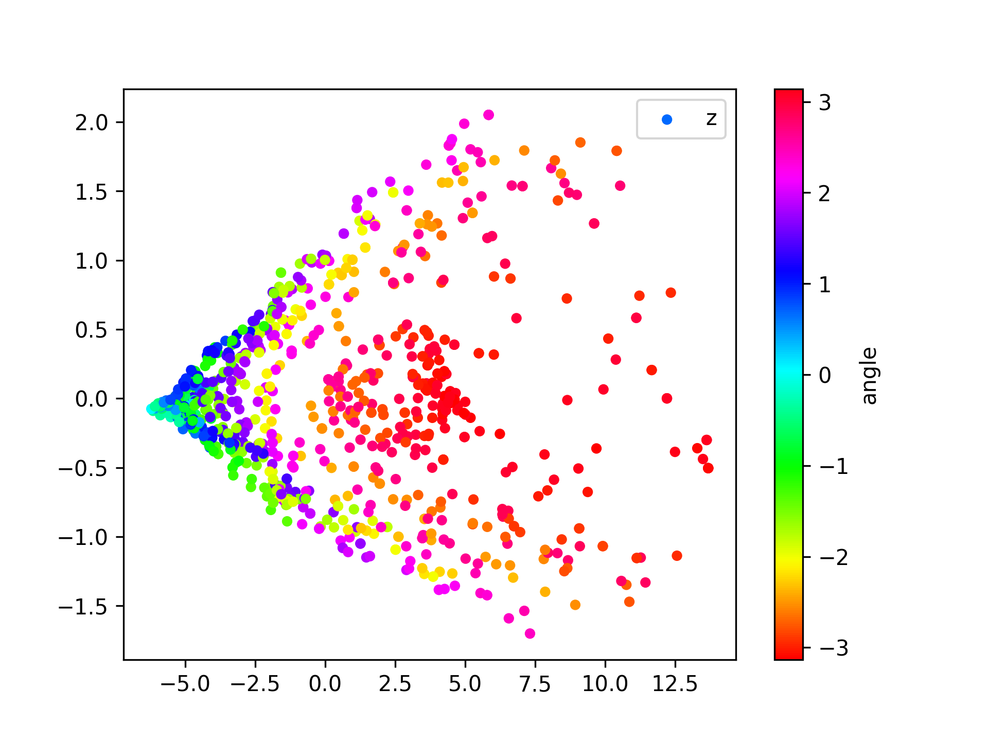
(e) FWRW

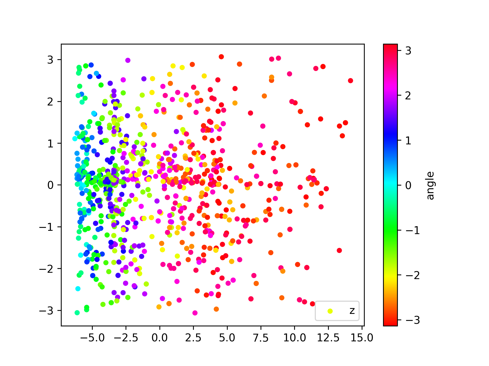
(f) FWRWIN

Figure 15: Learned state representations without distractors.

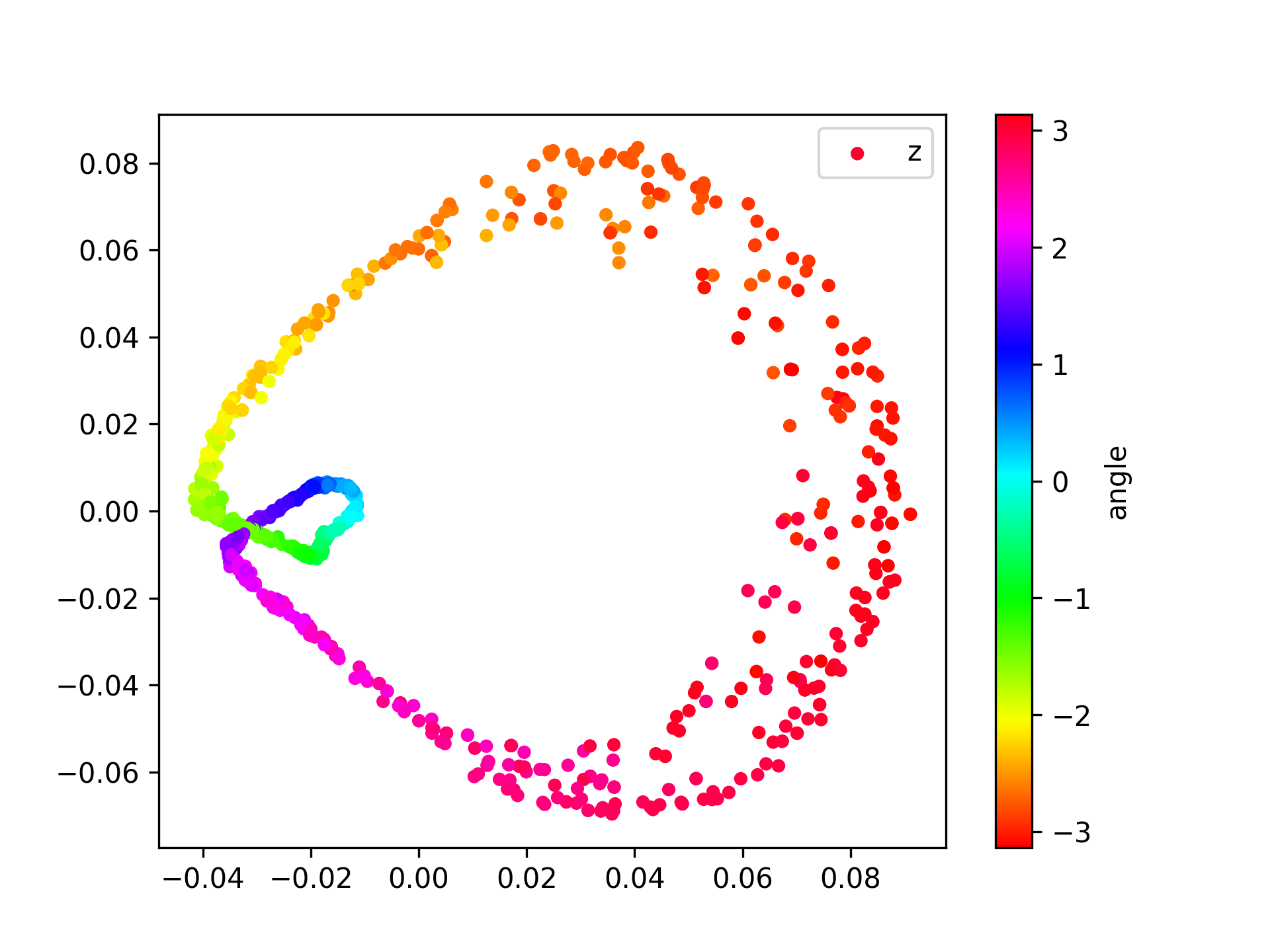
(a) PCA

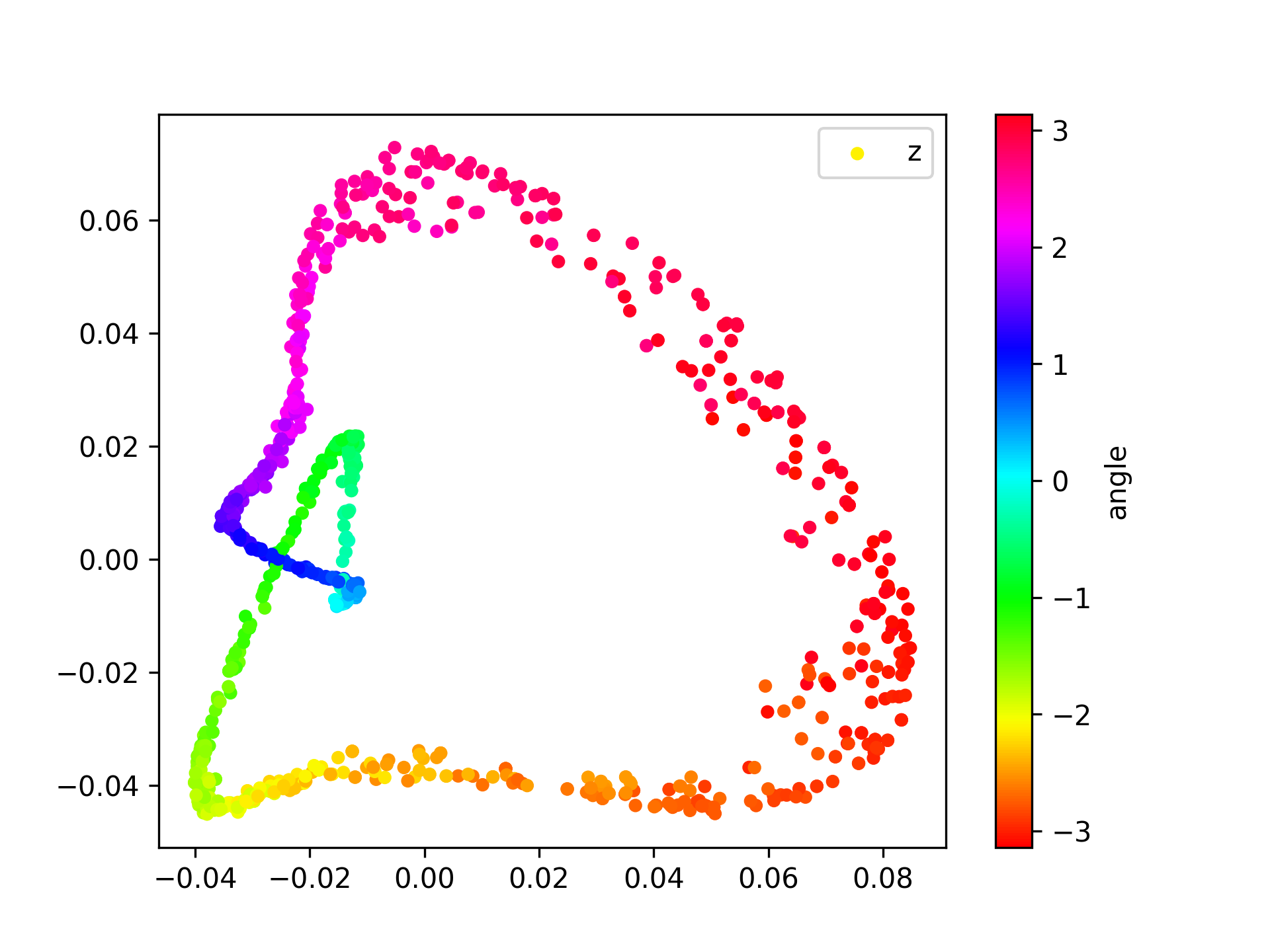
(b) AE

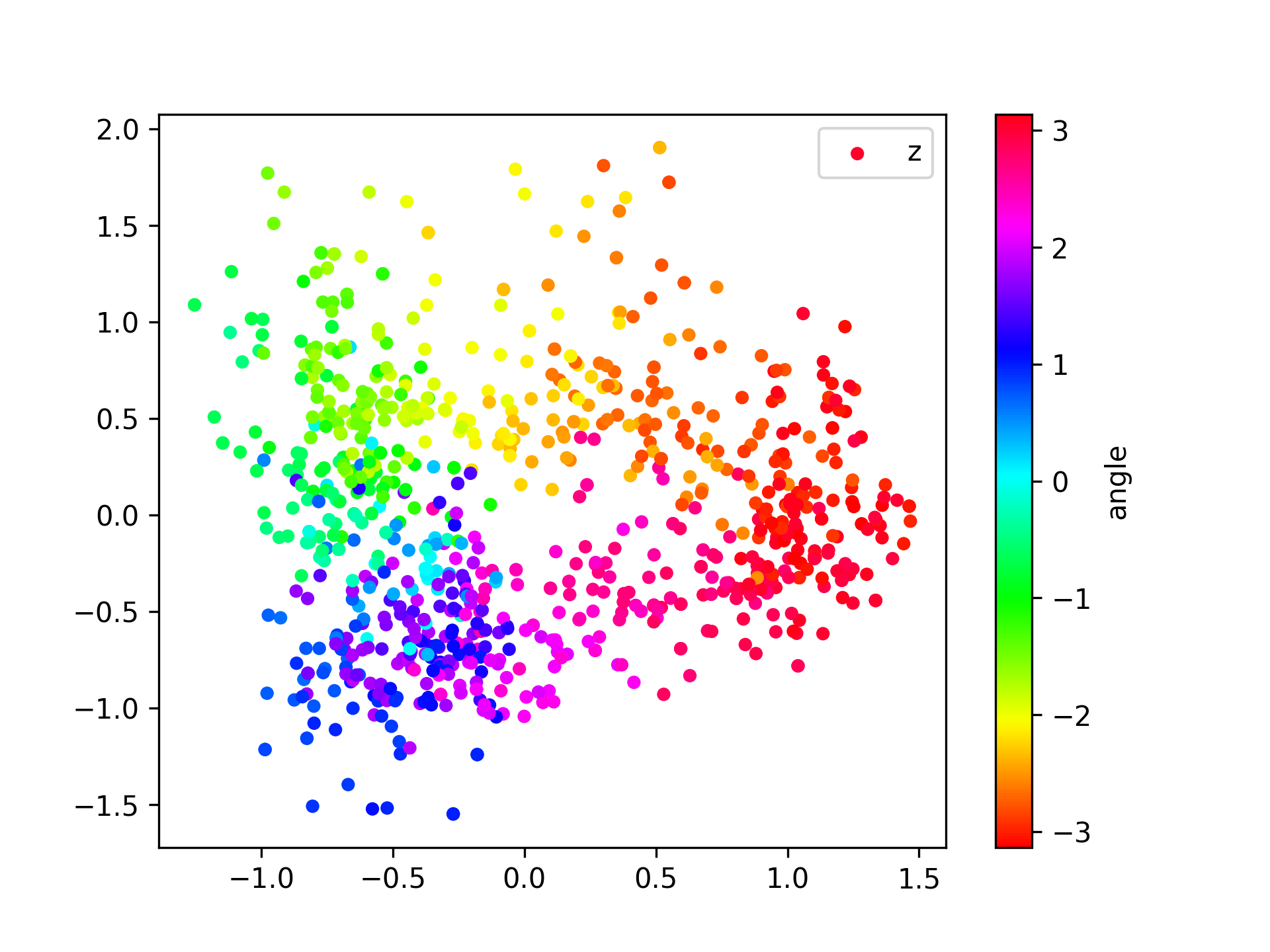
(c) VAE

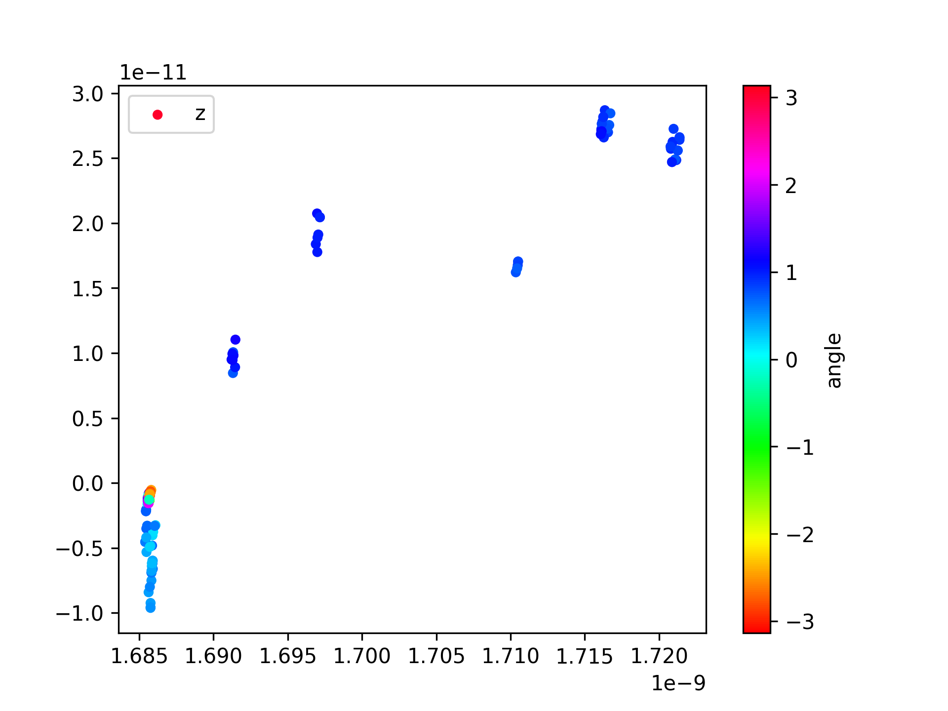
(d) FW

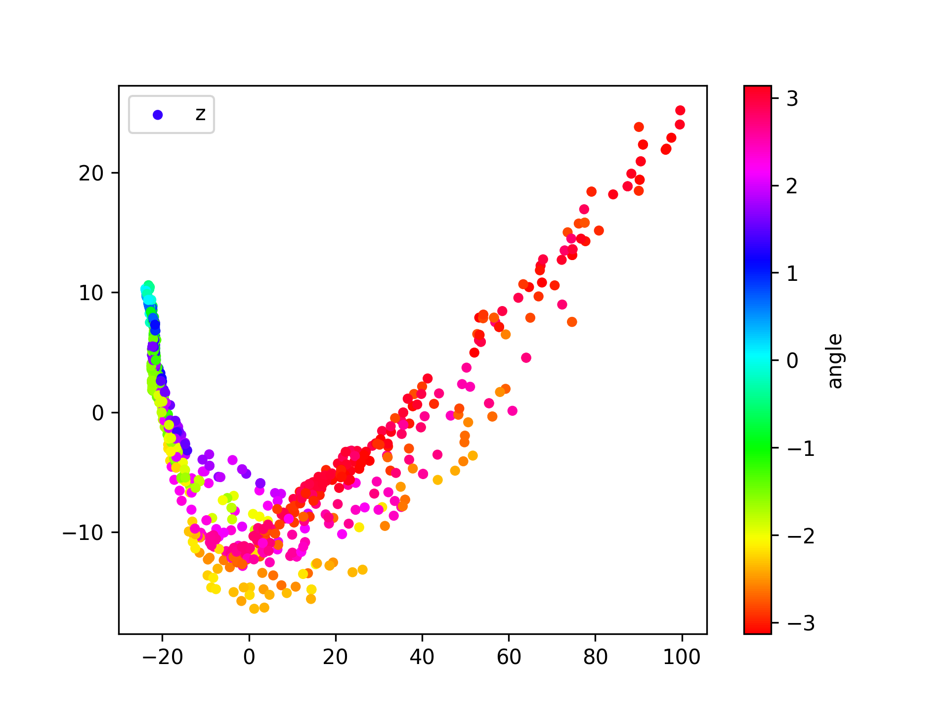
(e) RW

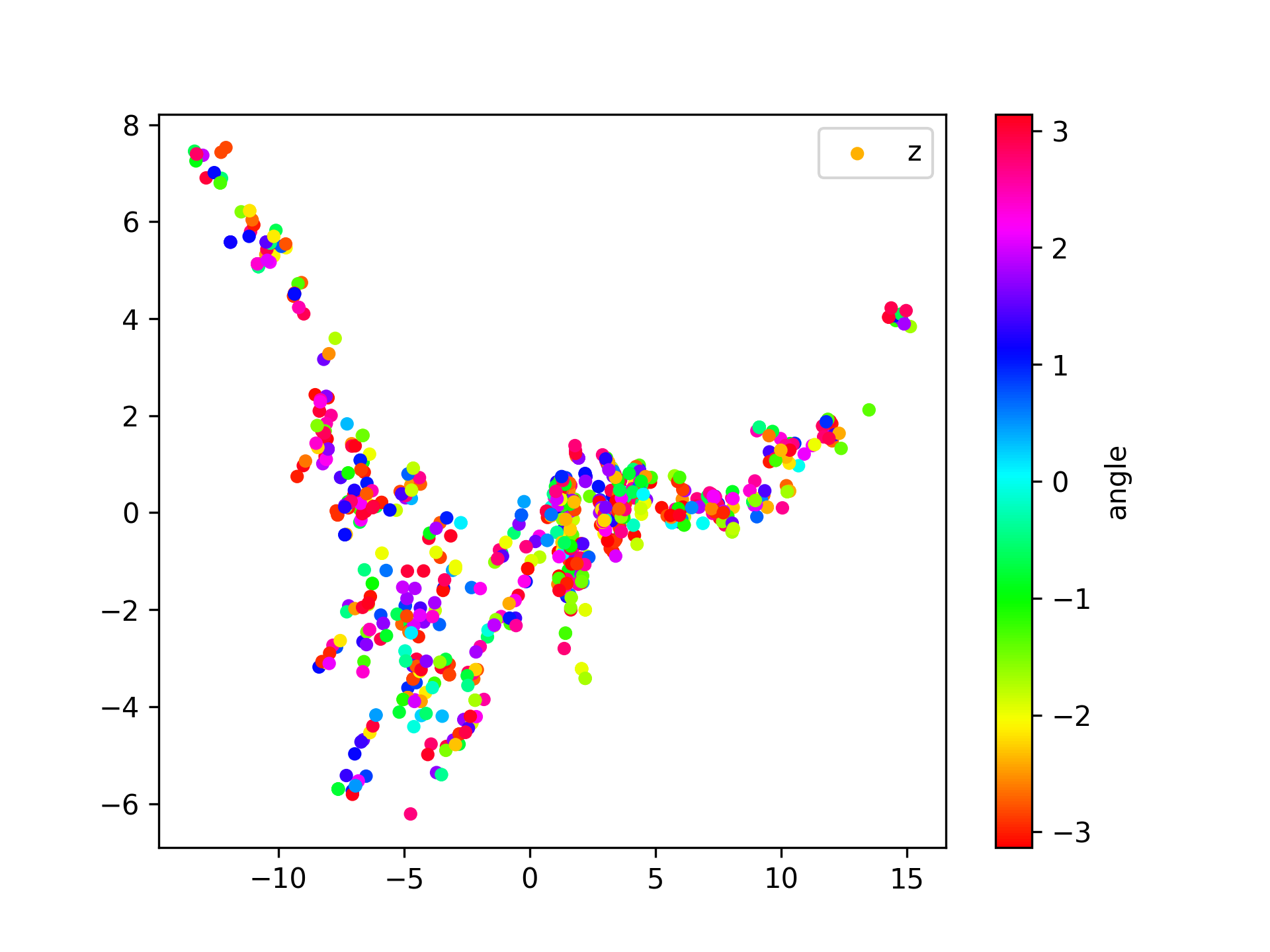
(f) IN

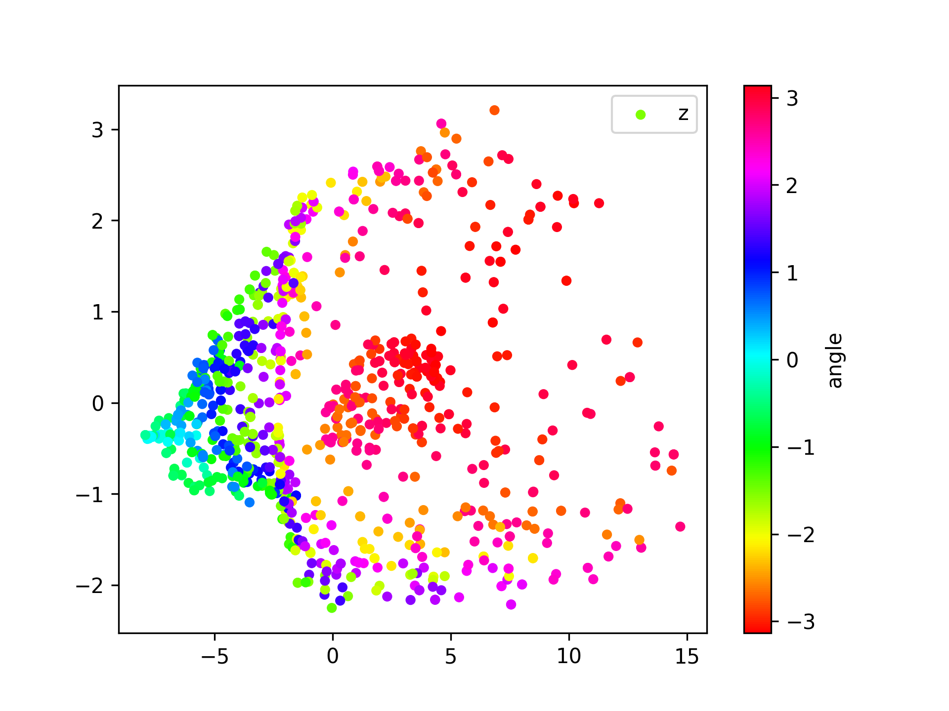
(g) MDPH

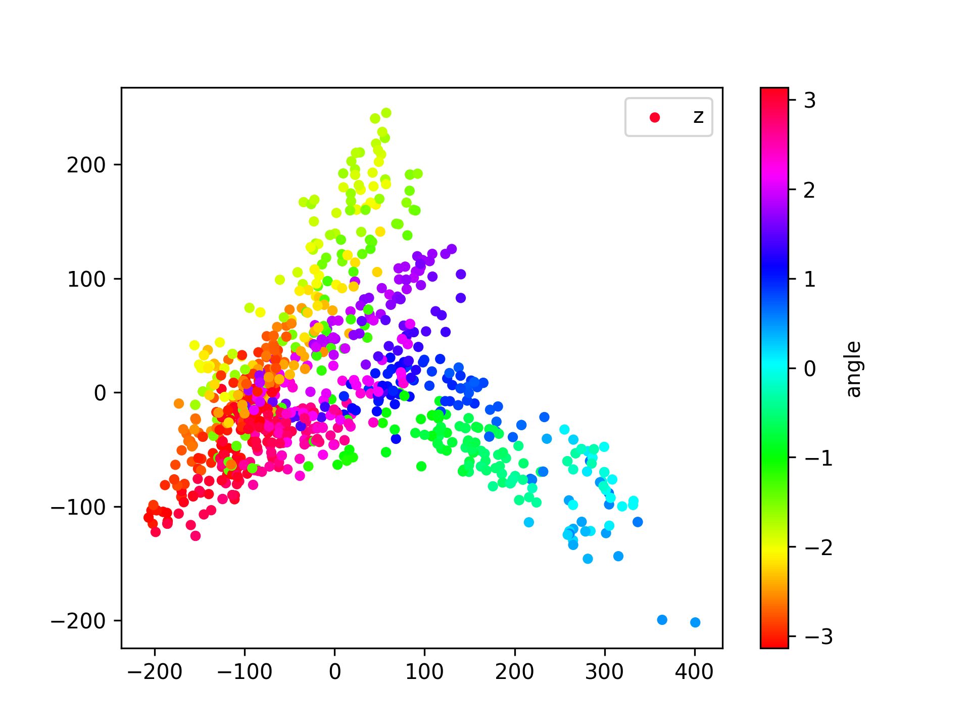
(h) BM

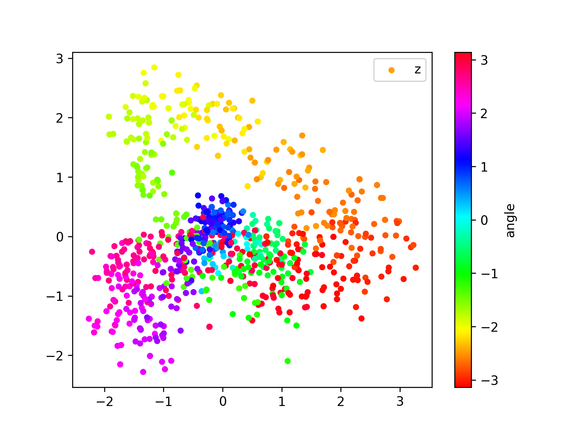
(i) PR

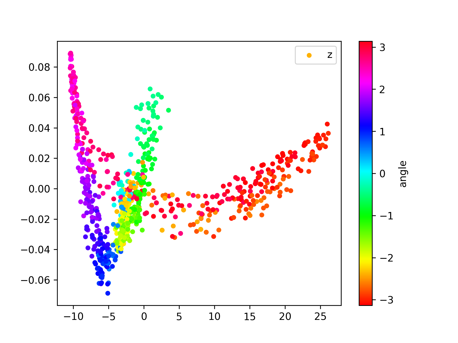
(j) CL

Figure 16: Learned state representations with fixed distractors.

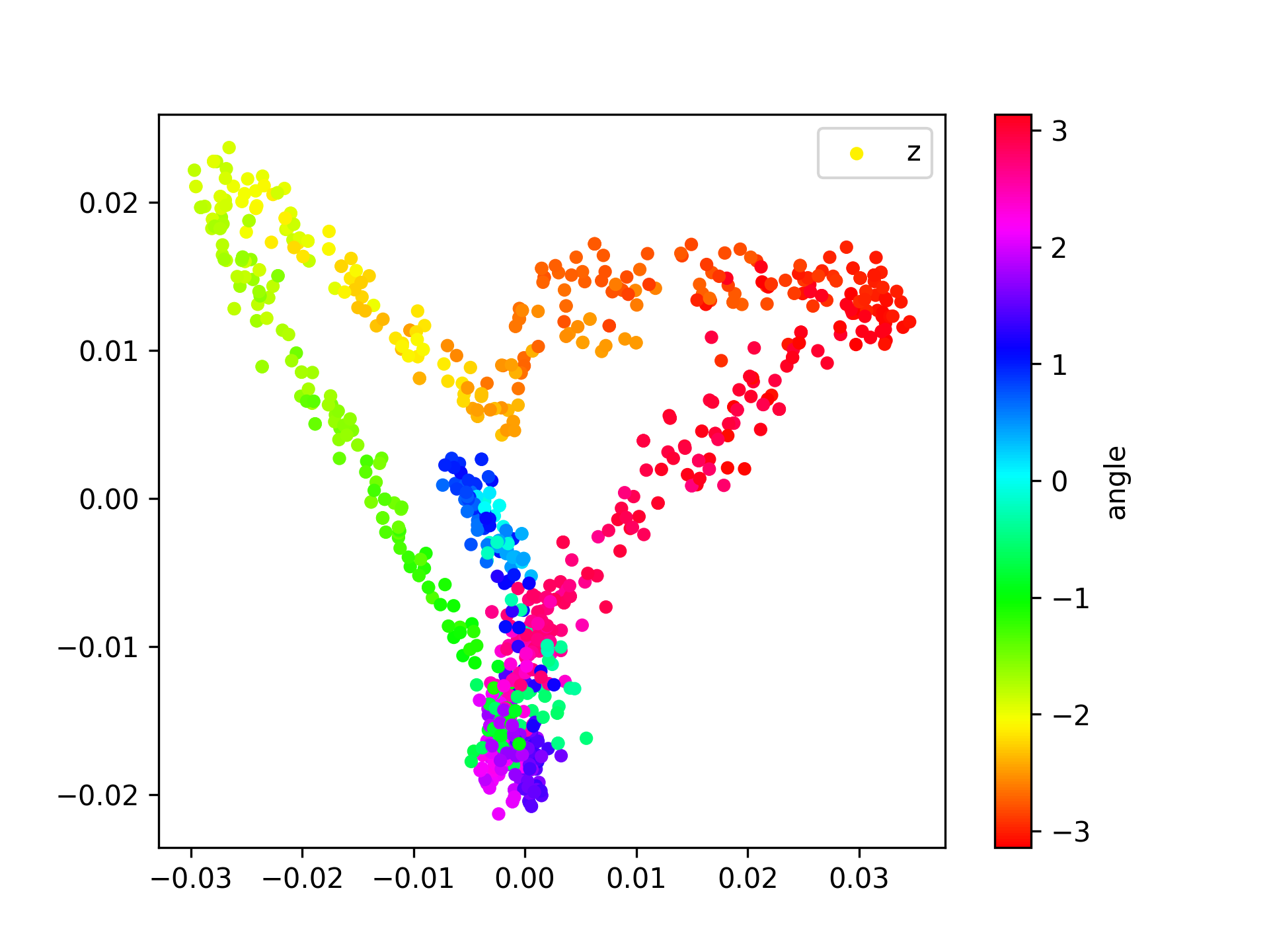
(a) AEFW

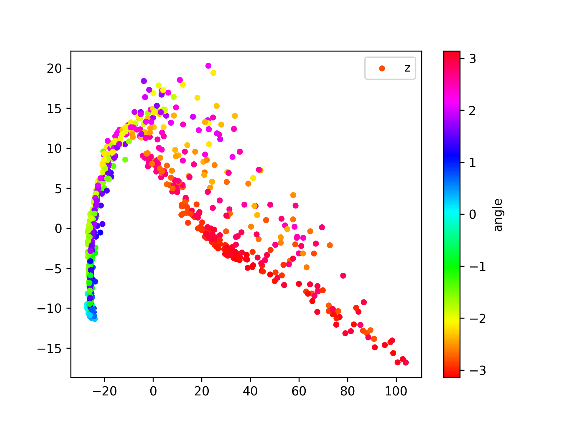
(b) AERW

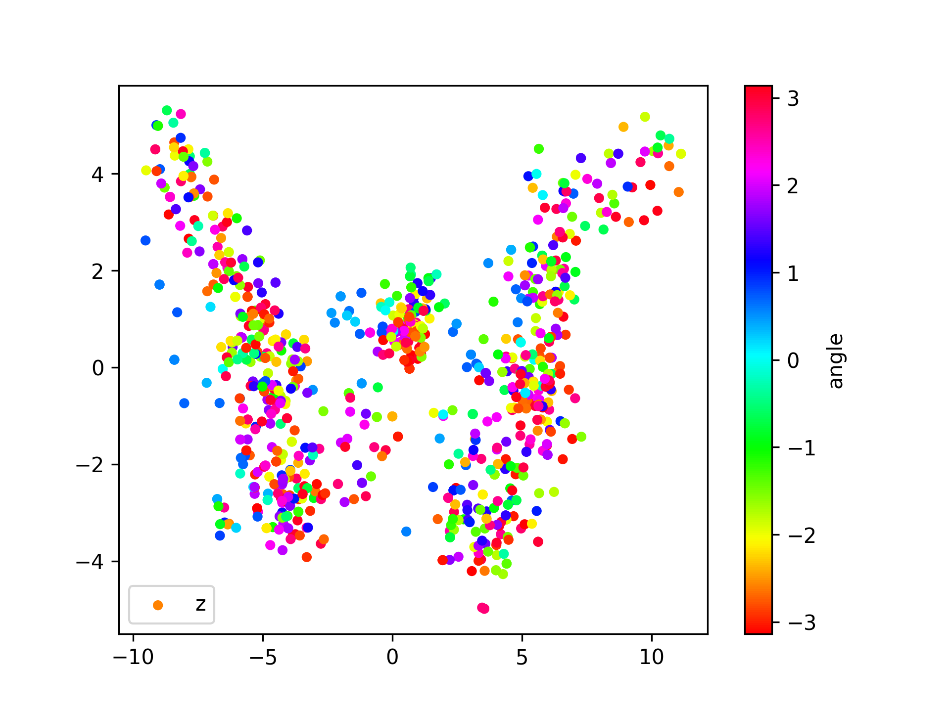
(c) AEIN

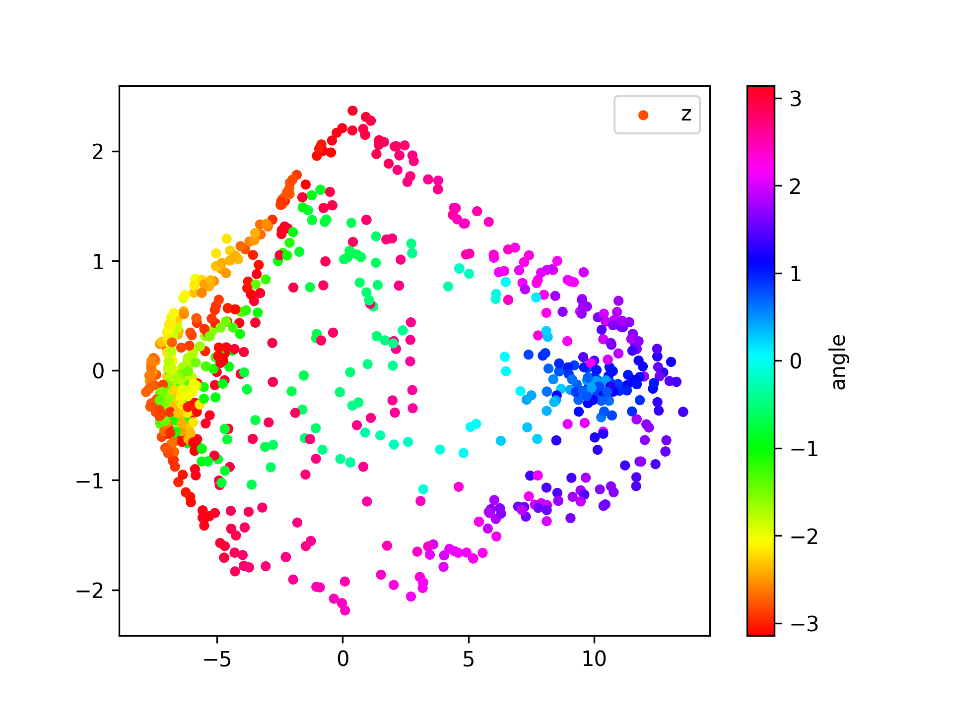
(d) FWCL

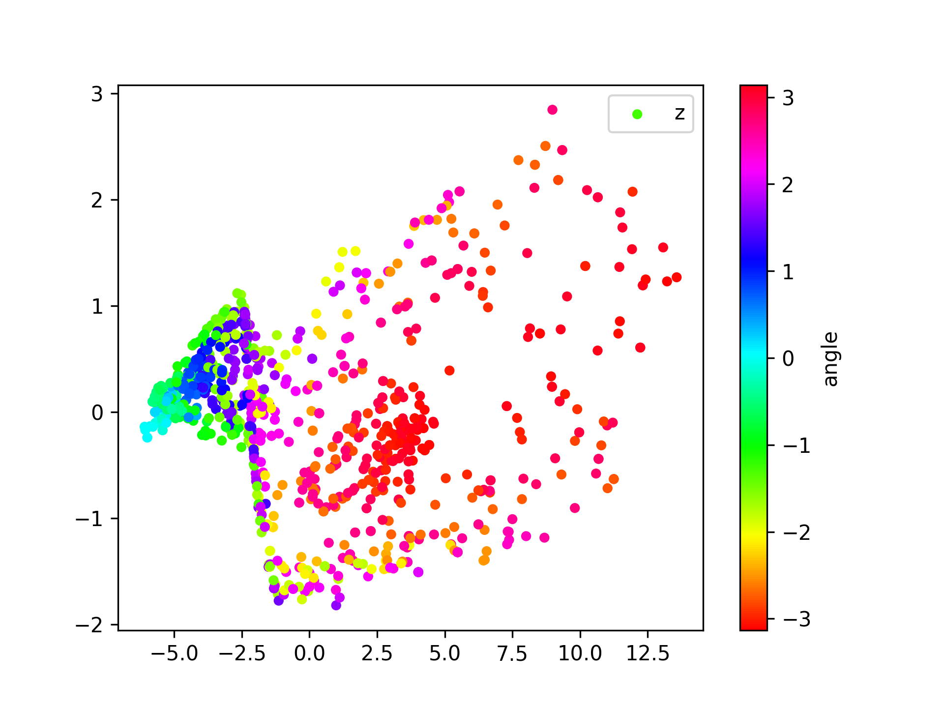
(e) FWRW

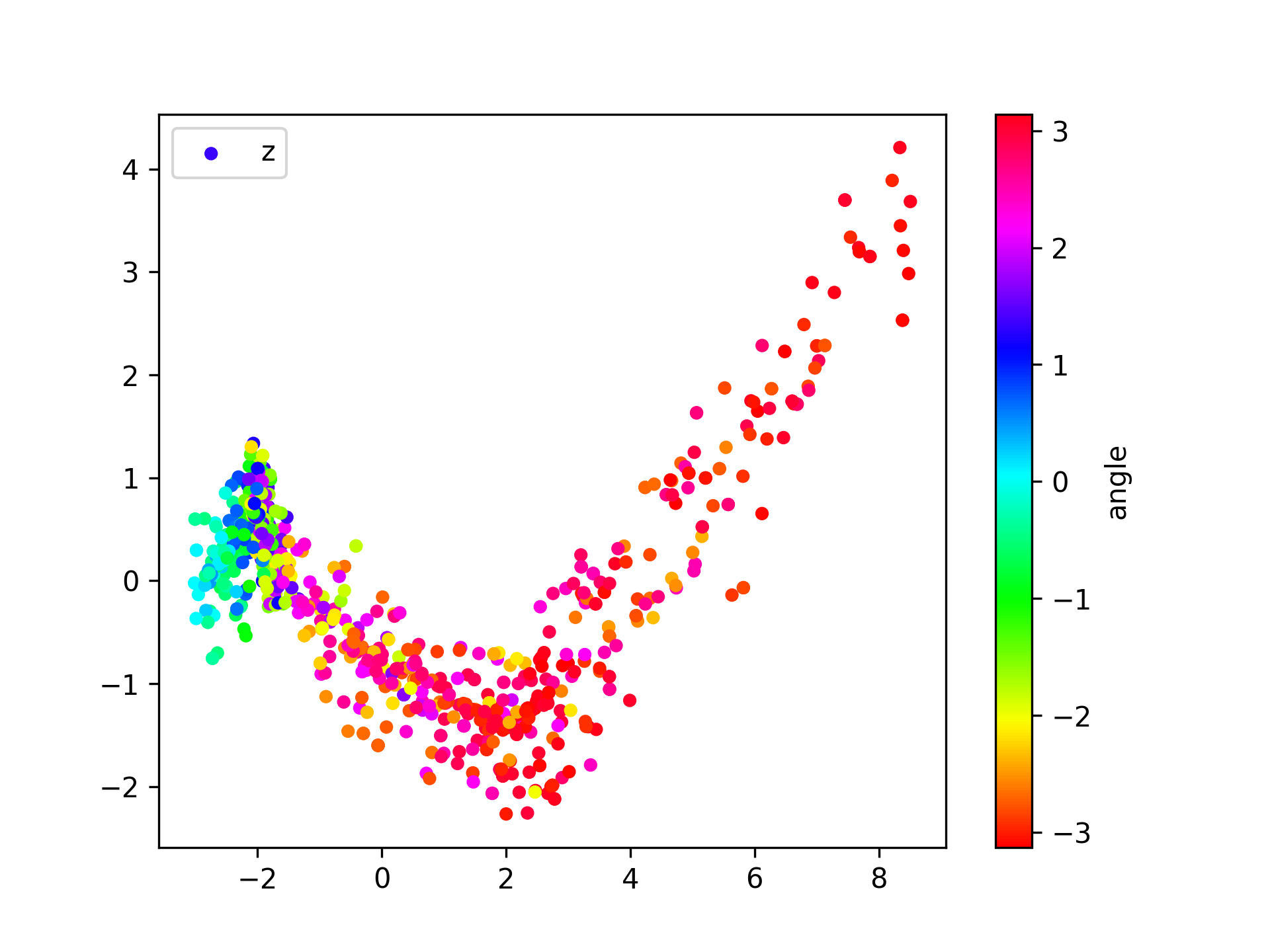
(f) FWRWIN

Figure 17: Learned state representations with fixed distractors.

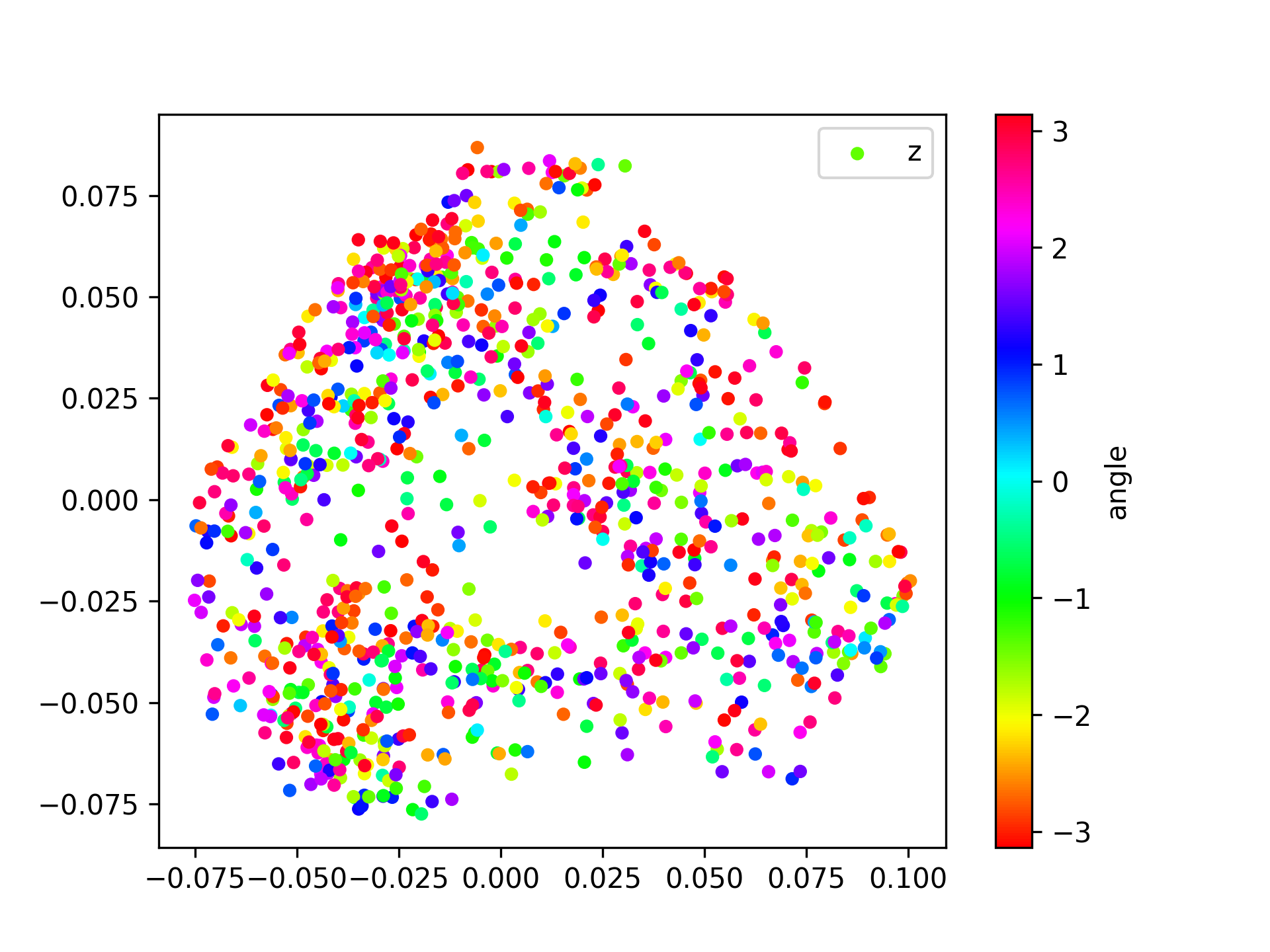
(a) PCA

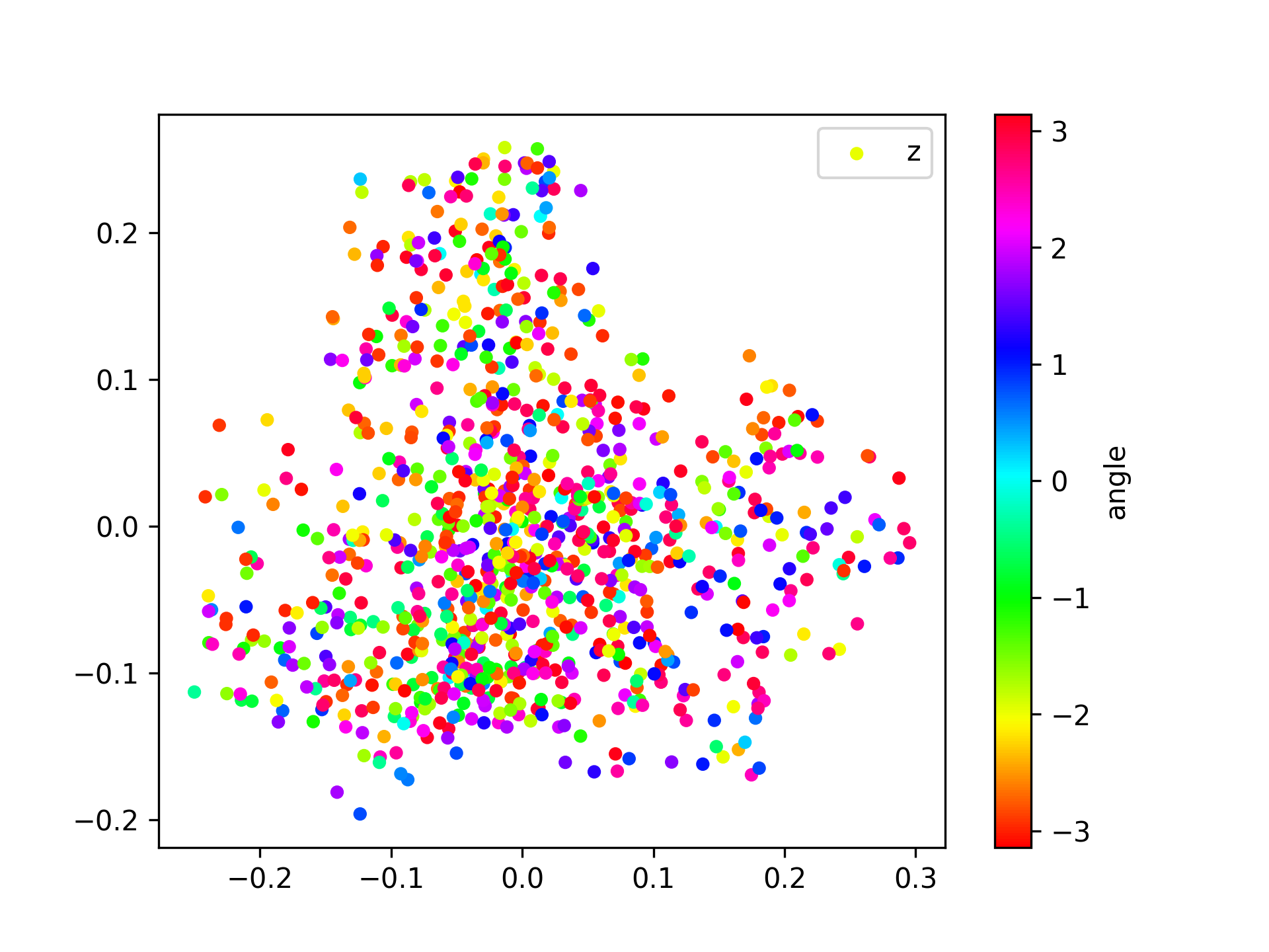
(b) AE

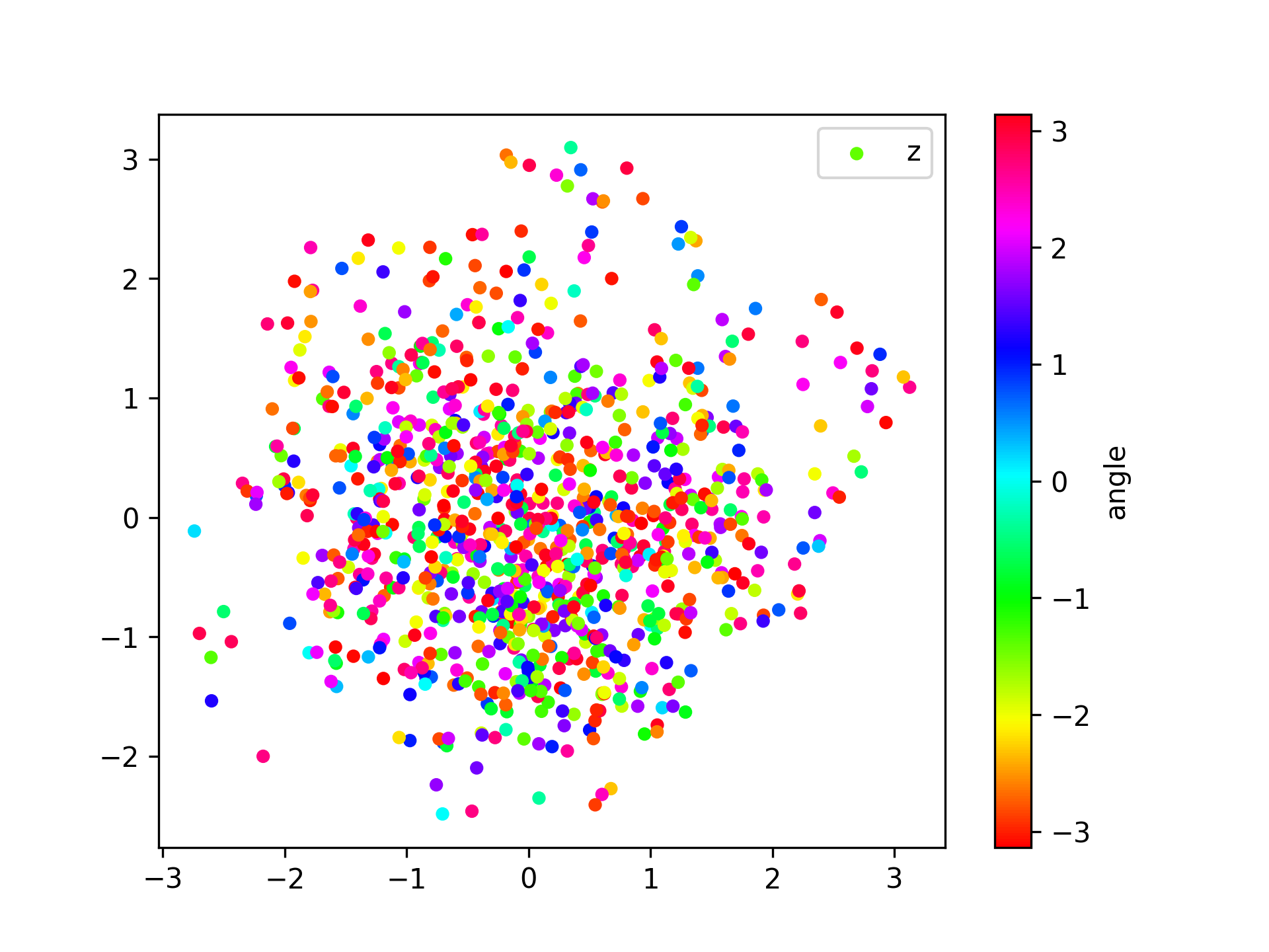
(c) VAE

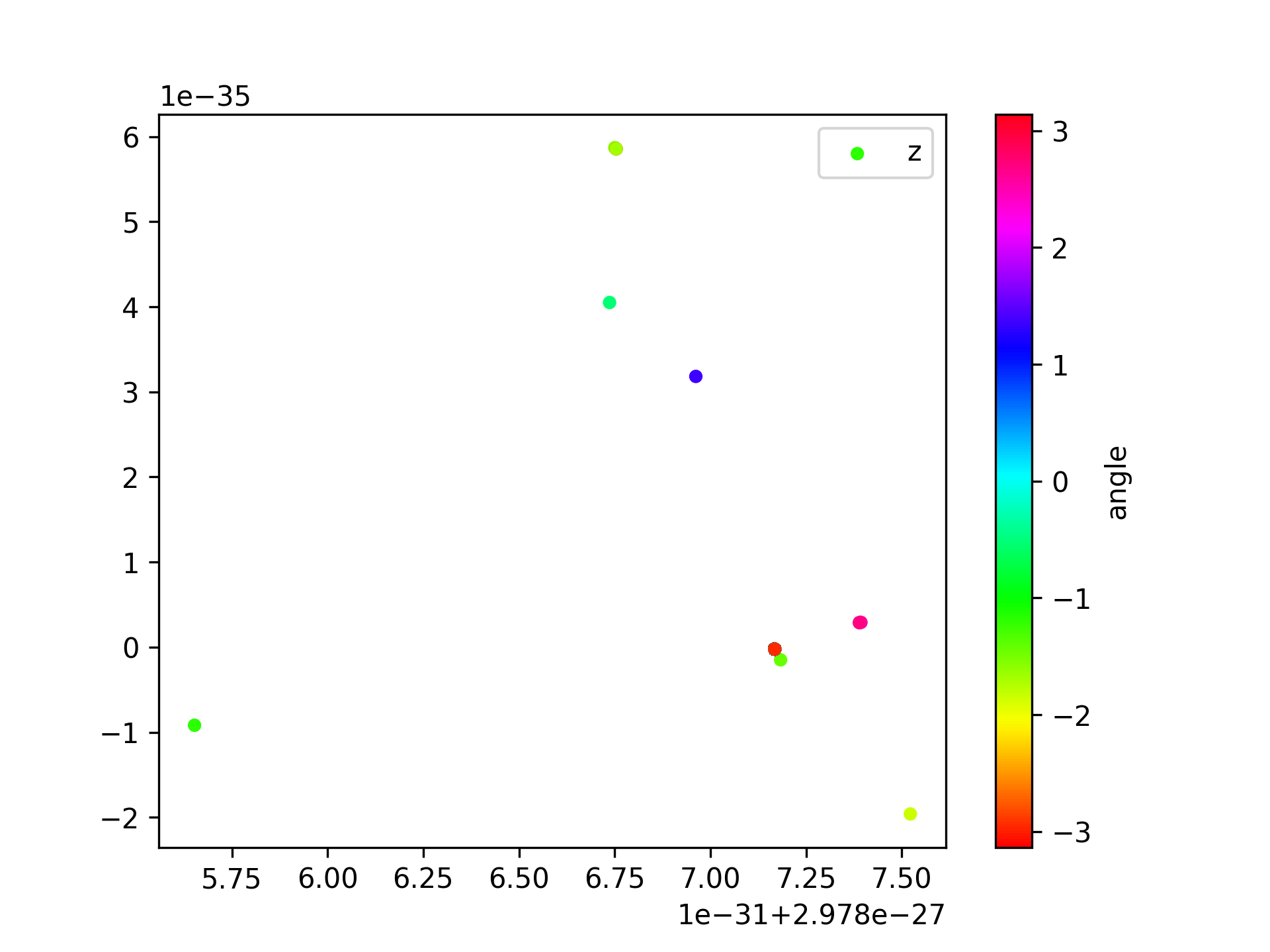
(d) FW

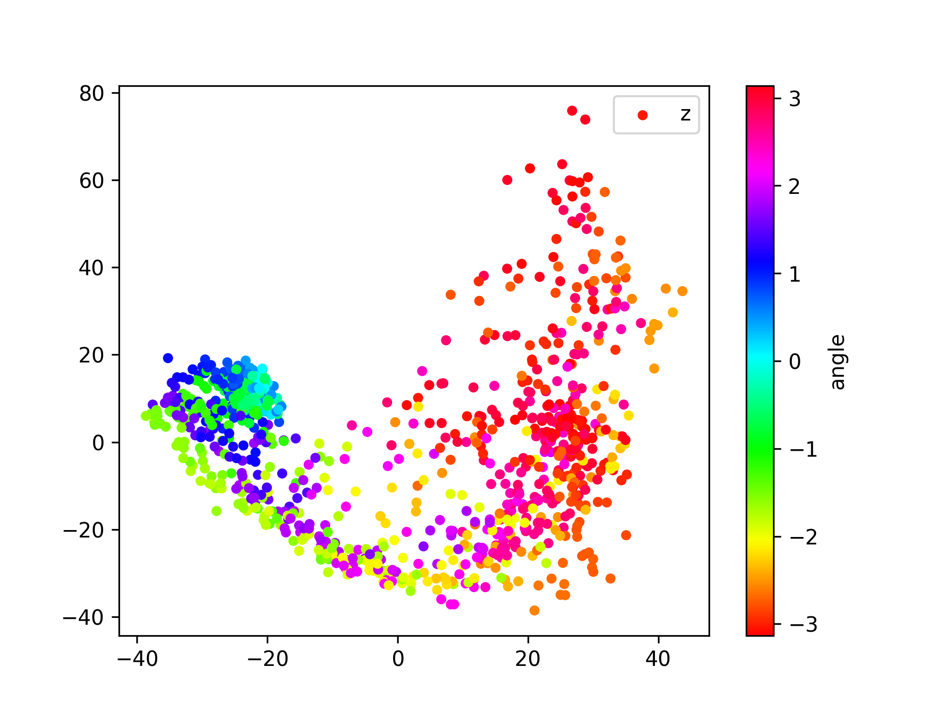
(e) RW

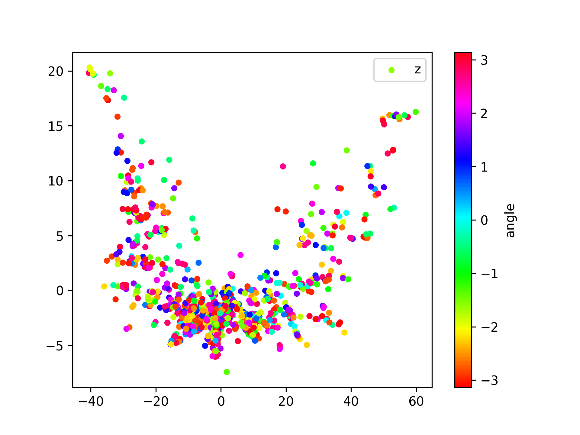
(f) IN

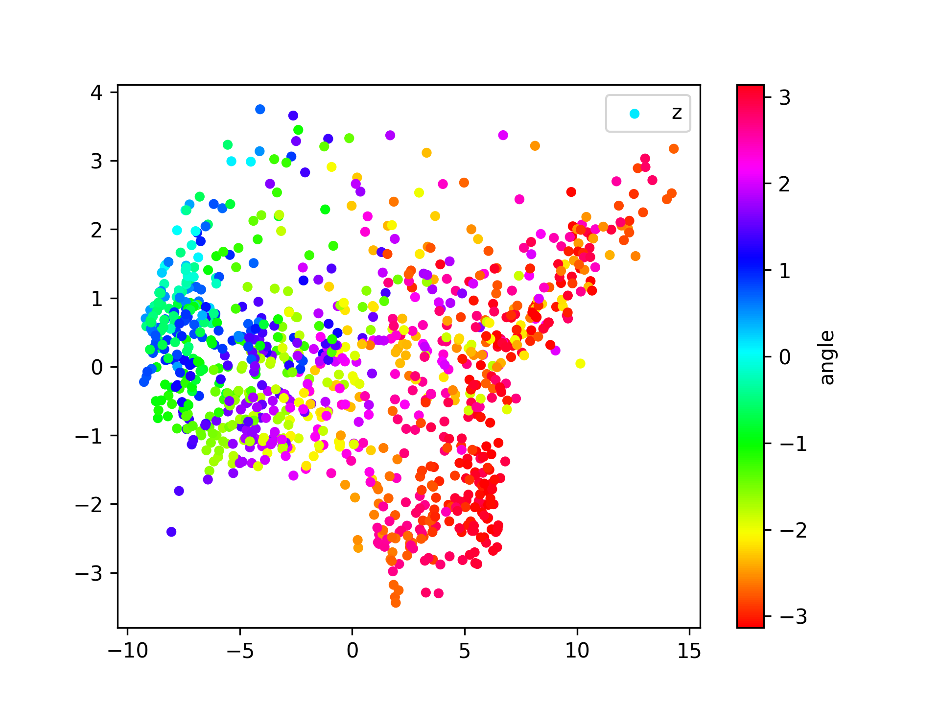
(g) MDPH

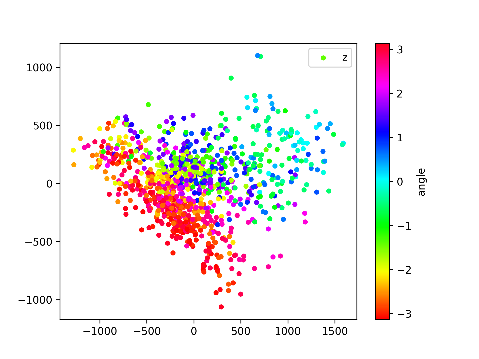
(h) BM

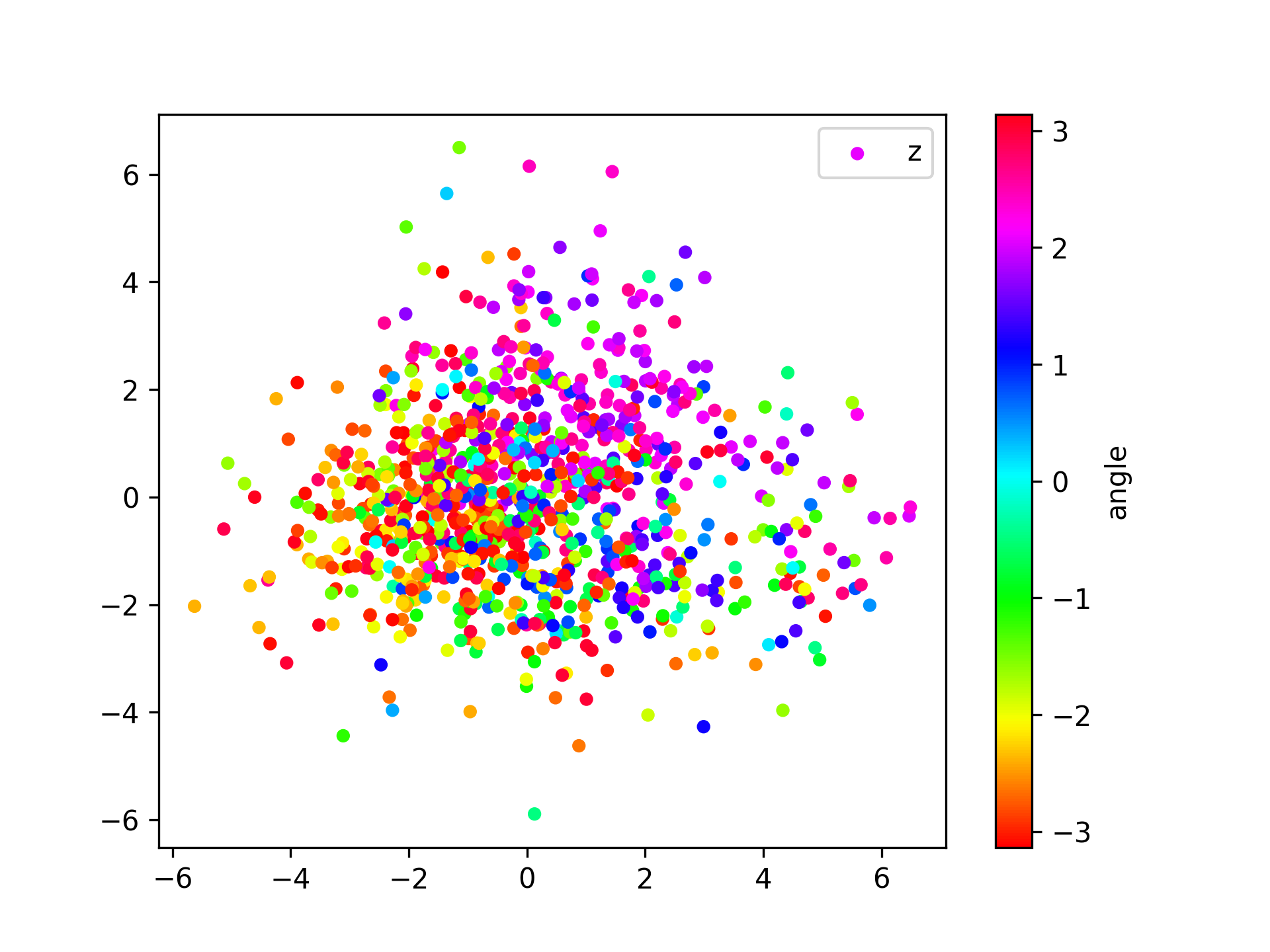
(i) PR

(j) CL

Figure 18: Learned state representations with randomly-positioned distractors.

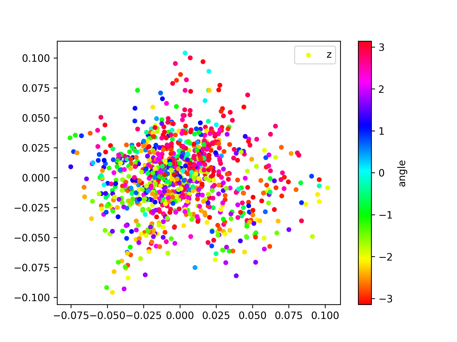
(a) AEFW

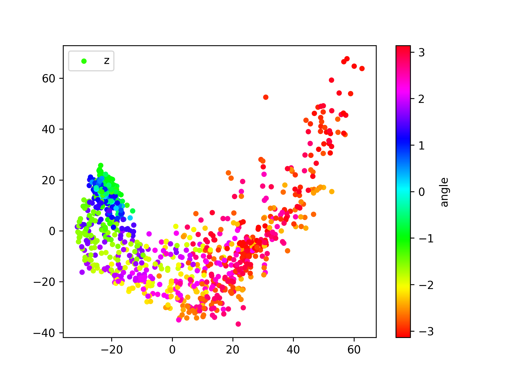
(b) AERW

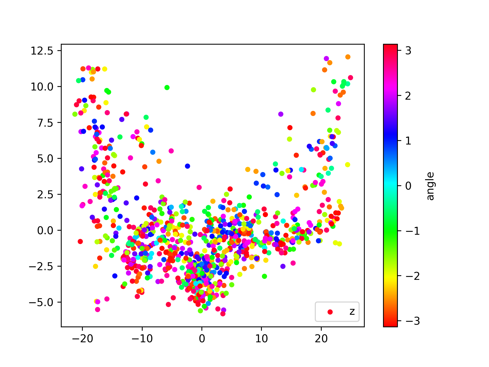
(c) AEIN

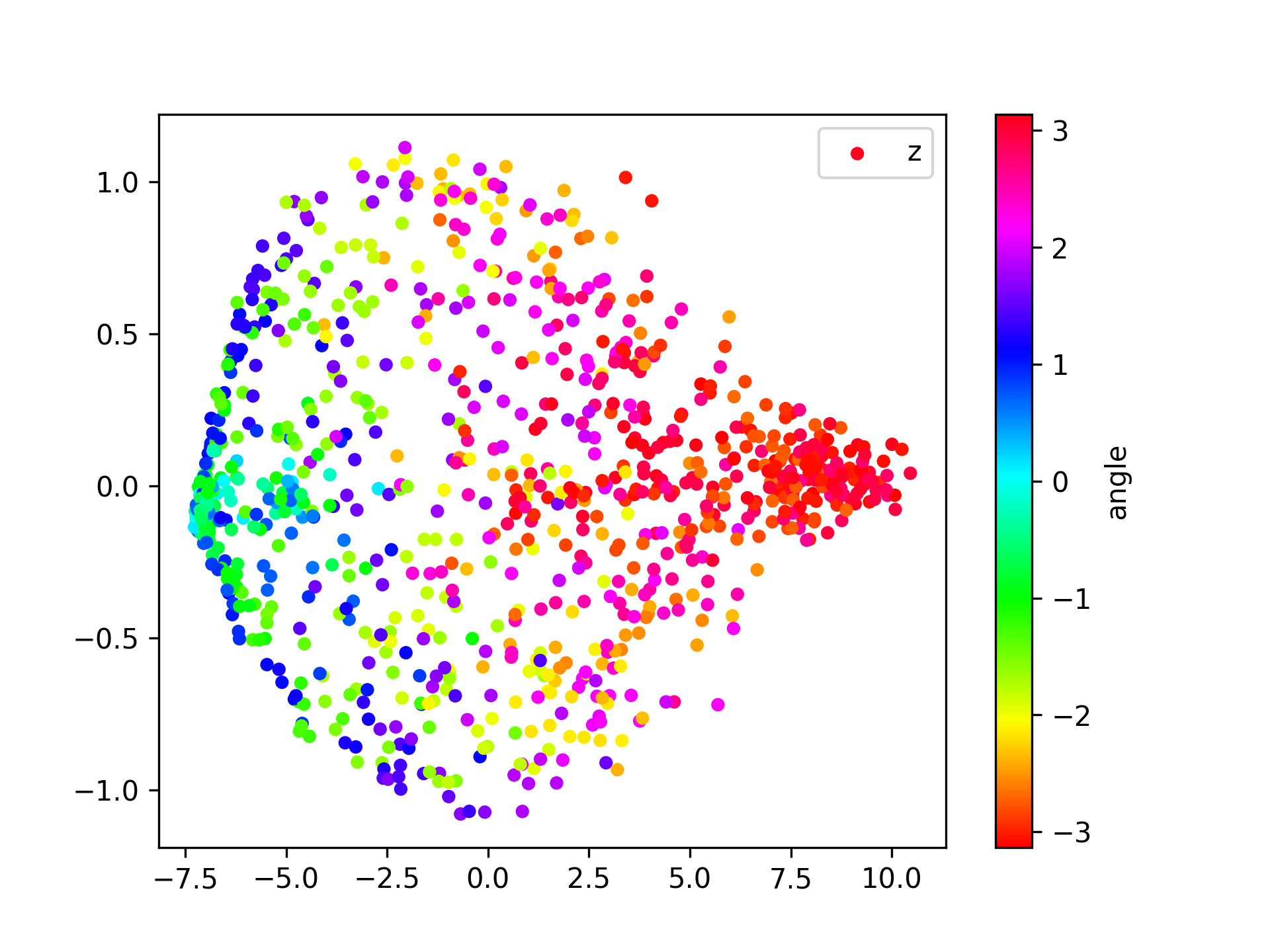
(d) FWCL

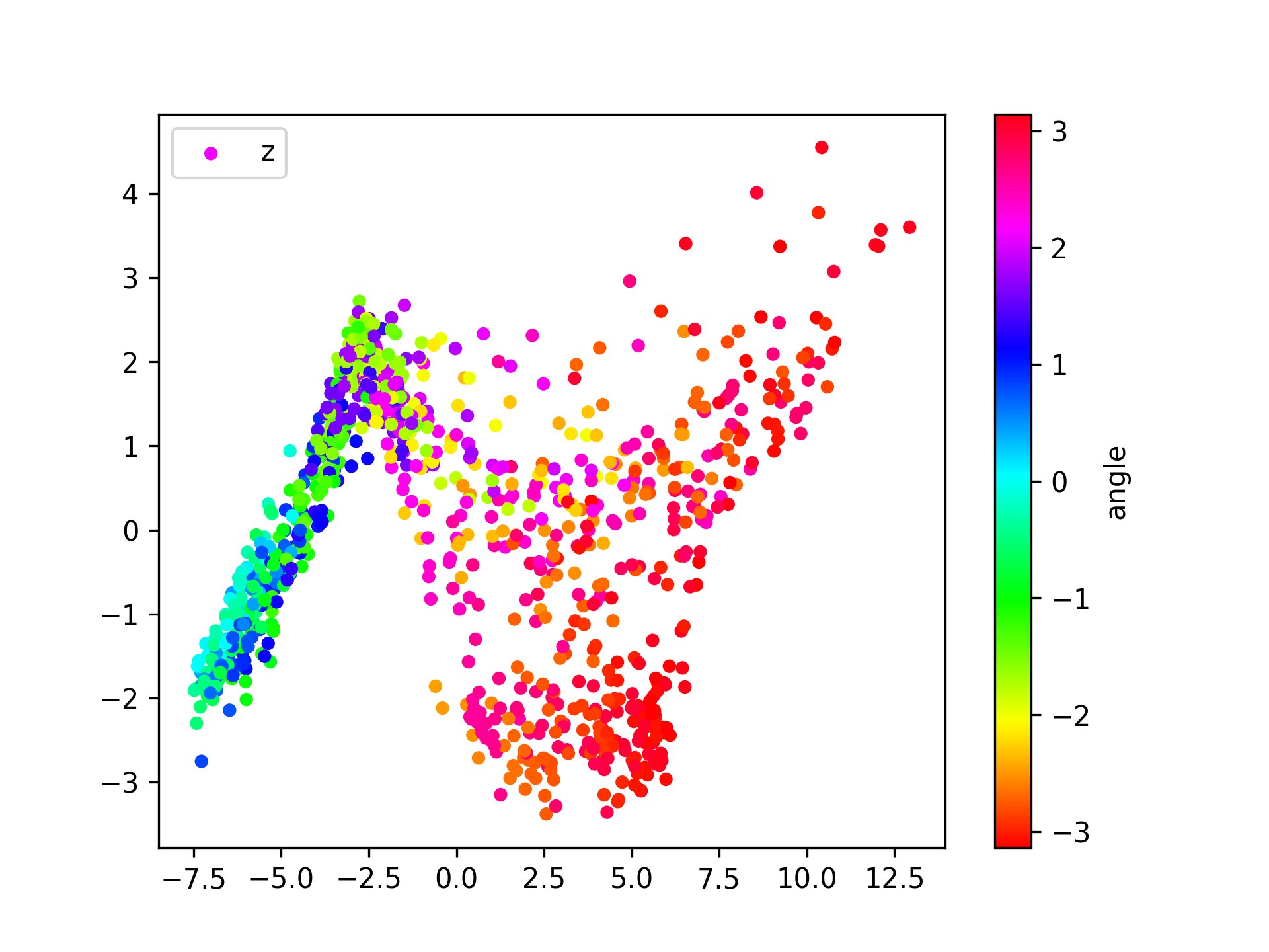
(e) FWRW

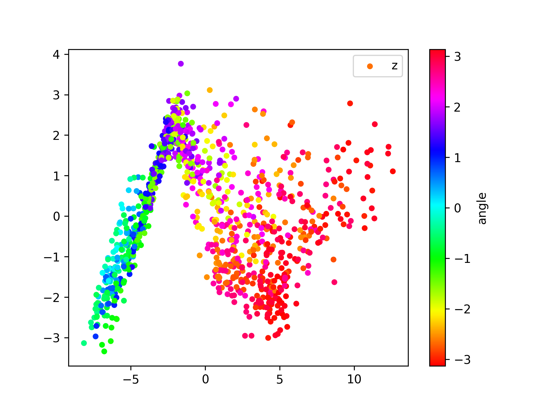
(f) FWRWIN

Figure 19: Learned state representations with randomly-positioned distractors.

In this section, we aim at briefly summarizing a key aspect of each category of methods:

• Pure observation reconstruction-based methods tend to struggle in encoding relevant features for control as the latent code may encode features useful for minimizing the reconstruction loss, e.g. backgrounds or distractors (see Figure 18(b)). However, this class of methods tends to have a more stable training procedure that hardly collapses.

• Approaches relying on MDP models naturally encode environment dynamics, but they tend to be harder to train, and they often need to be coupled with contrastive losses (e.g. in the case of the forward model) to prevent representation collapse (see Figure 14(d)).

• Priors allow higher sample efficiency than other methods but tend to suffer visual distractors and non-stationary environments (see Figure 18(i)).

• The reward model is crucial for smoothness, temporal coherence, and expressivity of the methods when randomly-position distractors are present. The reward model is a good discriminator of task-relevant and task-irrelevant information, especially in the case of non-sparse reward function (as in the pendulum example). With very sparse reward functions, the ability of the reward model to separate features is drastically reduced, and discriminating task-relevant and task-irrelevant information is an open challenge in the field. Additional mechanisms have to be often used, e.g. value function estimation.

• Contrastive losses are always combined with other losses, e.g. forward model loss [33] or temporal-difference loss [46], to improve sample efficiency and prevent representation collapsing.

4 Unsupervised Representation Learning in Deep Reinforcement Learning

When defining a taxonomy diagram for DRL methods, one of the first distinctions we have to address is how the samples collected via the interaction with the environment are used. Usually, we have two options: model-free and model-based methods. In model-free algorithms, the samples are used to directly estimate value function and policy, e.g. via temporal-difference learning or policy gradient [5]. In contrast, in model-based algorithms, the samples are used to build environment models, e.g. transition model or transition and rewards model, that are then exploited to estimate value function and policy analogously to model-free DRL.

For structuring our review, see Figure 20, we utilize these two classes of DRL methods, namely model-free and model-based, to define two macro objectives of the SRL approaches:

1. Increasing the sample efficiency, robustness, and generalization abilities of model-free DRL by learning meaningful low-dimensional state representations.

2. Improving prediction accuracy, robustness, and generalization abilities of learned latent MDP models and consequently the quality of the policies and value functions learned in model-based DRL.

Given these two objectives, we review how the approaches presented in Section Deep Learning for Learning State Representations are effectively used for improving end-to-end DRL algorithms.

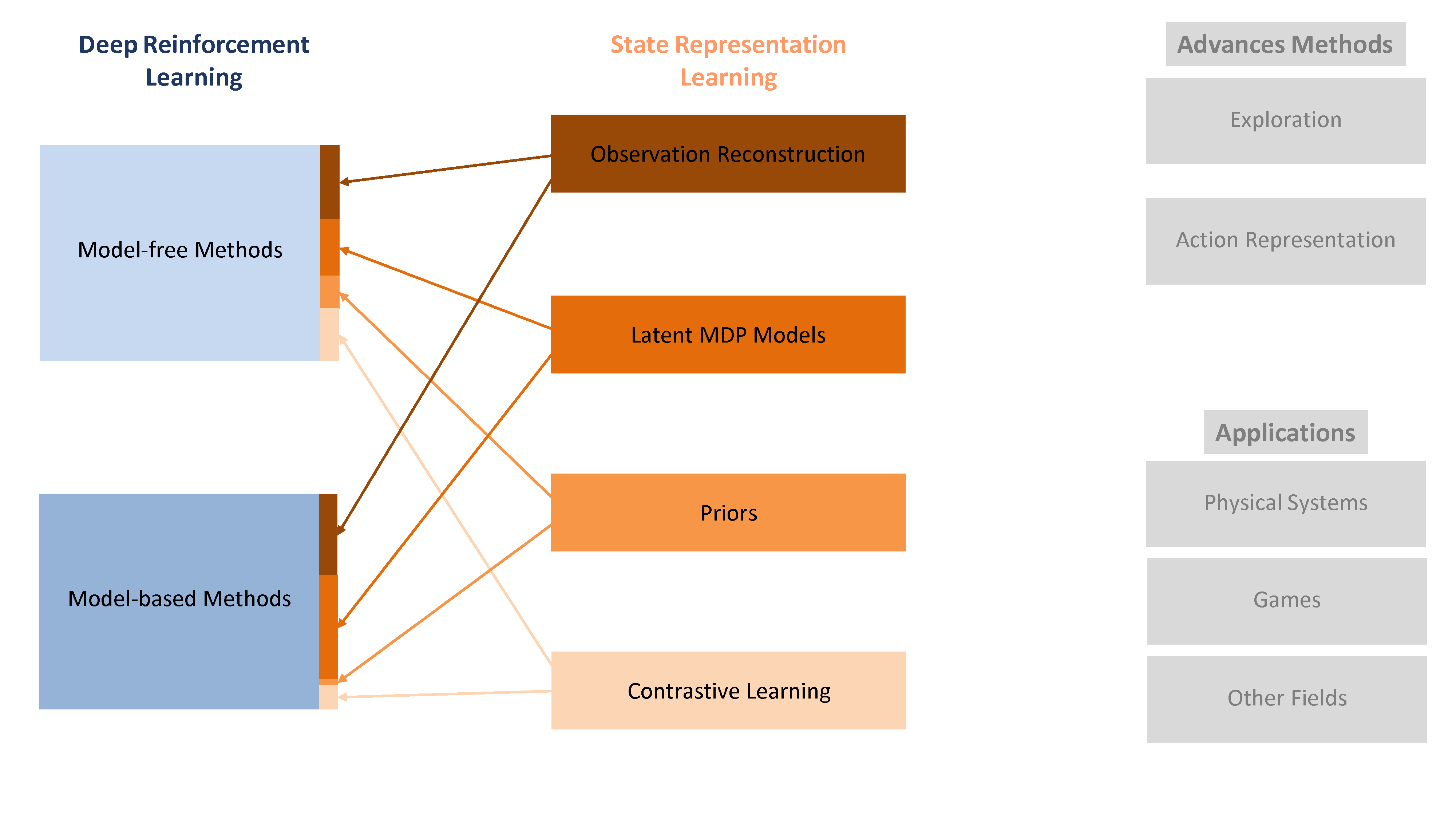
Figure 20: Overview of State Representation Learning methods in Deep Reinforcement Learning.

4.1 State Representation for Sample Efficiency in Model-free RL

This section discusses the problem of learning state representations for model-free RL. Such state representations are used by the agent to learn the value function and the policy by interacting with the environment.

4.1.1 Learning State Representations with Principal Component Analysis

One of the first applications of PCA in RL was proposed by [54], where a low-dimensional state representation was learned from raw grey-scale images. Using the state representation, the RL agent was efficiently trained to solve a single level of the game Super Mario Bros®. Another example of the use of PCA for learning low-dimensional state representation was the work of [55], where the return-weighted PCA (RW-PCA) was used to learn a state representation of a continuous grid world and the simulated robot tetherball game.

However, in complex problems, the linear mapping learned by PCA from observations to states is insufficient for encoding all the relevant information, and, commonly, non-linear and more expressive mappings are learned using the AE framework (described in Section Deep Learning for Learning State Representations).

4.1.2 Learning State Representations with Autoencoders

One of the first uses of AEs in RL was introduced in [56], where an AE is used to learn a 2D representation of a grid-world. The actual state of the environment was not observable, and the agent could only use grey-scale image observations corrupted by noise. The AE not only reduced the dimensionality of the observations to a 2-dimensional state vector allowing efficient RL, but also acted as a denoiser of the images. A similar example is the work of [57], where an AE was used to learn a compact state representation from grey-scale images of a real-world inverted-pendulum in the presence of time delays. The RL agent could quickly learn the optimal policy given the state representation, the previous action taken, and the delay. The last example of AE for SRL was shown by [58] where the AE was used for learning a compressed state representation of the game VizDoom [59].

When uncertainties have to be considered due to the stochasticity of the underlying MDP, AEs are often replaced by the VAEs (see Section Deep Learning for Learning State Representations). Examples of VAEs for RL could be found in the works of [60] using a beta-VAE in combination with a Denoising AE [61] to generate target observations for the reconstruction loss, [62], using a VAE for studying the problem of continual learning in continuously changing worlds, and [63] using a beta-VAE for learning a goal-based representation from the observation of goal states.

Despite these successes, AEs and VAEs are often not directly used in DRL because of two major limitations: (i) the reconstruction loss is often independent of the relevant features for control, and (ii) only the latent states are used in DRL, making the decoder an unnecessary element. In the following sections, we discuss how to tackle these two challenges.

4.1.3 Autoencoder Regularization with Auxiliary Losses

The lack of discrimination between relevant and irrelevant features for control due to the reconstruction loss translates into the lack of coherence and smoothness of the latent state space. For example, two consecutive observations that should be encoded close together in the latent space may be encoded by an AE far from each other if they present very different features. Therefore, AEs (and VAEs) need regularization via auxiliary losses.

In this section, we first present the approaches tackling the problem of learning the state representation in an offline fashion from batches of previously collected data. In offline approaches, the SRL model is first trained, and immediately afterwards its parameters are frozen. Eventually, the DRL algorithm is trained given a fixed state representation.

The first example is the Deep Spatial AE introduced by [64] for discovering compact state representations from RGB images in the task of learning dexterous manipulation using a robot arm. To improve the quality of the representation, next to the reconstruction loss, the authors proposed a regularization loss for keeping features from consecutive observations close to each other in the latent space. Similarly, the authors of [65] enhanced the VAE loss (see Equation (11)) with a forward model loss. Unlike other approaches, next to the state representation, the authors introduce an action representations too. In particular, each action is represented by a rotational matrix with four learnable parameters. Reward and inverse models were used by [66] for improving the AE-based state representation quality and allowing transfer learning from simulation to real-world (sim2real) in a mobile robot navigation task. A VAE regularized by a linear latent forward model was employed in [35] for learning low-dimensional representations of a pendulum and a robot arm for tactile manipulation. Similarly, a non-linear forward model in combination with an AE is used by [67]. VAEs with latent forward and reward models were used by [68, 69]. The latter used the forward model and the decoder to infer an approximate metric on the learned (Riemannian) manifold. The metric was used to penalize the uncertainties in latent states and latent dynamics. This penalization was added as an additional term in the reward functions to improve the training efficiency of the agent. The problem of imitation learning from third-person to first-person views was studied by [70]. A pair of AEs encoding third-person view observation and respective first-person view observation are regularized for disentangling view information from state space information using a permutation loss for matching third-person views to first-person views.

Alternatively, one could use the DRL loss as an additional regularizer for the encoder and train the neural networks online while interacting with the world (as in the case of end-to-end DRL). While these approaches more naturally update encoder and policy, they usually comes at the price of additional training instabilities as the state representation is not stationary anymore.

Online approaches were proposed by [71] where the Double DQN (DDQN) [72] loss, reconstruction loss, reward loss, temporal coherence loss, causality loss, and forward and inverse model losses were used. Another example is the work of [73], where a regularized AE [74] was combined with Soft Actor-Critic (SAC) [75], and [76], where a stochastic latent variable model was used in combination with a VAE and a forward stochastic model. In the context of multi-agent RL in partially observable settings, the authors of [77] proposed a recurrent AE combined with an Asynchronous Actor-Critic (A2C) [78] for learning the relations between the trajectory of the controlled agent and the trajectory of the modelled agent. The recurrent AE encoded sequences of observations and actions and produced a latent code that was used together with the raw observations as inputs to the A2C agent. Differently, the authors in [79] introduced a selectivity loss for specifically learning K controllable features using K independent policies. The selectivity of the features was defined as the expected difference in the representation of the next state and the current one. Selectivity can be interpreted as the reward for the control problem. The AE loss and the selectivity of the policy are jointly optimized to learn a navigation task in a grid world. Despite the novelty, this approach does not scale well with the size of the problem as K different policies have to be trained jointly. Unfortunately, K can vastly grow in complex scenarios.

4.1.4 Learning State Representations with MDP models

In RL, we are interested in learning task-relevant and compressed representations of the observations. The latent representations are used in most cases for learning the value functions and the policies, and the observation reconstructions are rarely used in practice, except for analyzing the results and for interpretability. In this section, we review approaches that do not rely on a decoder but only on auxiliary losses using the latent MDP models. The methods in this section are online approaches.

The first important aspect is the MDP homomorphism (see Section Deep Learning for Learning State Representations). The MDP homomorphism allows us to define a metric to train the encoder without needing a reconstruction loss and guaranteeing a Markovian latent space when the loss functions approach zero. In this category of approaches, we find the work of [37], where the MDP homomorphism metrics were formulated as loss functions and used as regularizers for a distributional Q-learning agent [80]. In most Atari games, the approach outperformed different baselines, such as end-to-end DRL and AE-based approaches.

A closely-related concept to the MDP homomorphism is the so-called bisimulation metric. Here we find the work of [81, 82, 83, 43] combining the bisimulation metric with high-dimensional observations for learning-low dimensional representation for discrete and continuous MDPs. Minimizing Lax Bisimulation and MDP homomorphism metrics guarantee a Markovian latent space homomorphic to the true MDP in terms of transition and reward function. However, two major problems arise from using these two metrics: (i) collapsing of the state representation to a trivial one in case of sparse reward functions, and (ii) learning of the forward model is often hard in practice.

Traditionally in DL, the collapsing of the representations is prevented using contrastive losses pushing negative embeddings apart (see Section Contrastive Learning). Contrastive losses are often used in approaches that do not rely on a decoder and are more prone to representation collapse. InfoNCE loss and momentum encoders [84] were used in combination with SAC and Proximal Policy Optimization (PPO) [85] by [50], SAC and RainbowDQN [86] by CURL [46], distributional Q-learning by [87], and PPO by [88] for continuous and discrete control problems. In contrast, the authors in [89] introduced PI-SAC that, similarly to CURL, used the InfoNCE bound to capture the mutual information between two random observations as an auxiliary task for continuous control from pixels. However, differently from CURL, PI-SAC captures information about the future states. Additionally to the InfoNCE, [51] added a forward model loss and a mutual information loss between the current latent state and the next latent state to add further structure to the state representation and improve the accuracy of the forward model. A return-based contrastive loss is used by [90] in combination with a state and action embedding, SAC and RainbowDQN, while [91] uses a triplet loss for learning state representations of robot behaviours from video demonstrations in combination with the PILQR algorithm [92].

Instead of relying only on the forward, reward, or contrastive losses, many authors proposed different combinations of multiple objectives in addition to the DRL algorithm loss. One of the earliest methods introduced by [93] combines the A3C loss [78] with a reward model and a pixel control loss for learning a Q-function to change the pixel values maximally. Similarly, in the context of robot navigation, [94] uses A3C with additional objectives for inferring depth maps from RGB images and detecting loop closure. In [95], the authors combine the PoPArt-IMPALA [96] with a recurrent encoder, a forward model, predicting the latent states from the history of observations, and a reverse model, where the reverse model predicts the history of observations from the latent states. IMPALA [97] is also used by [98] in combination with a recurrent forward model for belief estimation. [36] combines forward and inverse models for learning to poke with the Baxter robot in the real world. In contrast, [99] uses a goal-aware cross-entropy loss for discriminating goals in the context of multi-target DRL. In [100], the authors use an inverse model loss with a mutual information loss to learn a provable Markovian state abstraction without needing forward and reward models.

4.1.5 Learning State Representations with Priors

Instead of relying on the learning of the MDP models that are often hard to learn, it is possible to shape the loss functions used to train the encoder to incorporate known properties of the actual environment state (see Section Priors). Differently from the case of the latent MDP models, the approaches relying on the priors are offline.

The so-called robotics priors were introduced in [28, 16]. These loss functions were inspired and shaped accordingly to simple physical laws in the context of robotics. An example of regularization provided by the robotics priors is the proportionality loss, placing pairs of state embeddings close to each other if generated by consecutive observation and connected by an action. In [101], a new set of priors was introduced. Differently from the previous set, the authors proposed priors regularizing the positions of the state embeddings and their velocities, i.e. variations between two consecutive states, to be close to each other in consecutive states better to exploit the underlying smoothness of the physical world. In [53], the authors introduced a new set of robotics priors exploiting action structures in continuous action spaces, a common scenario in robotics, while in [102] the set of original priors from [28] were extended to multi-task learning with the addition of a task-coherence prior pushing apart embeddings from different tasks. In [45], the robustness of the original priors was tested in the presence of visual distractors and domain randomization. The authors introduced the so-called reference-point prior compensating for the degrading of the performance due to the rapid changes in the environment background. The reference-point prior uses true state samples as references for patching together the different embeddings from different trajectories The robotics priors have been extended to deal with POMDP by [15]. To do that, the authors introduced the so-call landmark prior that extends the reference prior from [45] to multiple reference points. Using multiple reference points is crucial for regularizing the different trajectories in the latent space. The robotics priors do not use any task-specific information in the reward function. One could argue that the state representation has to incorporate information about the goal. On this line of thought, the authors of [103] introduced a new set of priors enforcing similarities and dissimilarities of state pairs using the rewards collected in each state. These reward-shape priors are a natural way to incorporate task-specific knowledge in the state representation.

4.1.6 Learning State Representation without Auxiliary Models

Improving the quality of the state representation can be done without additional objectives. An example is the work of [104] where the Behavioural Cloning (BC) [105] loss was used for training the encoder. Two consecutive state embeddings were concatenated to form the vector that was fed to the DRL networks. A similar approach was used by [106] where consecutive state embeddings from a stack of frames were concatenated together with their latent flows, i.e. the difference of pairs of consecutive embedding, to form the augmented state vector that was used by the DRL algorithm. The authors of [107] proposed a framework for learning a context representation using the history of image stacks and force sensor readings for learning to push objects using a robot arm in combination with Qt-Opt [108]. The context representation was concatenated with the encoder features and fed to the DRL algorithm.

4.1.7 Summary

In this section, we aim at briefly summarizing a key aspect of the methods:

• Most of the reviewed contributions rely on the (V)AE or on the CL frameworks. AE and CL are essential elements for SRL in DRL by providing the foundation for learning different latent MDP models. MDP models that, when used alone, are prone to representation collapsing.

• Non-SRL objectives that we named in the table "other objectives" are often included when learning the representations, especially in an online fashion. These objectives are often the DRL algorithms objectives, such as minimization of the TD error or maximization of the reward.

• In contrast, despite being often done in practice, the policy objective was empirically proven to be detrimental to the learning of the state representation [73].

• One could also think of combining many different methods to obtain the best representation, e.g. in [71]. However, training the encoder using multiple loss functions needs additional care in balancing the different terms. An unbalanced total loss may cancel some of the gradients of single losses.

In Table 2, we summarize the contribution presented in this section and we highlight the methods from Section Deep Learning for Learning State Representations that each contribution employs.

Table 2: Which SRL methods are used by each contribution?

Method ($\rightarrow$) Contribution ($\downarrow$)	PCA	AE	VAE	FW	RW	IN	MDP H	BM	PR	CL	Other Objectives
[54]
[55]
[56]
[57]
[58]
[59]
[60]
[61]
[62]
[63]
[64]
[65]
[66]
[35]
[67]
[68]
[69]
[70]
[71]
[73]
[76]
[77]
[79]
[37]
[109]
[81]
[82]
[83]
[43]
[50]
[46]
[87]
[88]
[89]
[51]
[90]
[91]
[93]
[94]
[95]
[36]
[99]
[100]
[28]
[16]
[101]
[53]
[102]
[45]
[15]
[103]
[104]
[106]
[107]
[108]

4.2 State Representation for Accurate Latent Models in Model-based RL

In this section, we review the most relevant model-based DRL methods for learning predictive state representations through latent forward models in Section Learning State Representation with Latent Forward Models or latent forward and reward models in Section Learning State Representation with Latent Forward and Reward Models.

4.2.1 Learning State Representation with Latent Forward Models

Embed to Control (E2C) [110] used a VAE for learning a low-dimensional latent state space that was used as input to a linear latent forward model for obtaining a linear reduced-order model of a system from high-dimensional observations. The linear forward model forced the encoder to encode features that linearize the latent state space dynamics. VAE and the latent forward model are jointly trained together. After learning the reduced-order model, the control was performed via model-based techniques relying on the learned model, such as iterative linear quadratic regulation and approximate inference control. The authors of [111] proposed a similar approach to E2C. However, a non-linear latent forward model was combined with an AE. Model Predictive Control (MPC) was used to control the system. Another example is the work of [112], where again an AE with non-linear forward dynamics was emplyed with the addition of latent-space consistency loss. The consistency loss enforces that the latent states are close to the embedding of their next observation, providing further regularization to the latent state space.

The State Space Models (SSMs) [113] introduced an approach for learning deterministic and stochastic state representations for state estimation in the context of model-based RL. The deterministic SSMs (dSSMs) used an AE or a VAE in combination with a deterministic forward model, while the stochastic SSMs (sSSMs) used a VAE in combination with a stochastic forward model. Differently from many works in the literature, the stochastic forward model did not directly approximate $\bm{z}_{t+1}\sim p(\bm{z}_{t+1}|\bm{z}_{t},\bm{a}_{t})$, but made use of a latent variable $\bm{\eta_{t+1}}\sim p(\bm{\eta}_{t+1}|\bm{z}_{t},\bm{a}_{t},\bm{o}_{t+1})$ to predict the next latent state $\bm{z}_{t+1}=T(\bm{z}_{t},\bm{a}_{t},\bm{\eta}_{t+1})$. The approach was tested on the Atari Learning Environment (ALE) [114], and the policy was learned using the state representation via Imagination Augmented Agent [115]. Similar approaches to sSSMs, combining VAEs and stochastic forward models, were introduced by [116, 117, 118, 119], but with the sole goal of proper state estimation and the control was left as future work.

All the prior approaches relied on a vector representation of the latent states. However, encoding observations as vectors is not the only option. One could think of exploiting inductive biases and encoding the observations as nodes of a graph. Contrastive Structured World Model [31] encoded the latent states as an element of a graph and used a non-linear forward model approximated by a Message Passing Graph Neural Network [120, 121]. Another approach embedding observations into a graph is Plan2Vec [122], where the graph was constructed by learning the distance between the nodes, i.e. the latent states and a search algorithm is used to learn the shortest path on the graph from the current state to a goal state.

4.2.2 Learning State Representation with Latent Forward and Reward Models

The problems of continuous control, state representation learning, and latent models learning were tackled by PlaNet [123] and Dreamer [124], where a recurrent VAE with stochastic latent forward and reward model was learned. The policy was learned via MPC by PlaNet and via actor-critic DRL by Dreamer. Control via MPC was employed in [125] after learning a task-agnostic state representation using an AE, a linear forward model relying on the Koopman operator [4], and a reward model. Discrete control was done in [126] via predictive autoencoding and a reward prediction model for learning to play the Atari games in a model-based fashion using PPO.

The learning of a plannable MDP homomorphism was proposed by [33], using a similar approach to [37]. However, the authors of [33] additionally learned an action representation and used a contrastive hinge loss (see Section Deep Learning for Learning State Representations) to prevent the state representation from collapsing due to sparse rewards. After learning the state representation, latent forward and reward models offline, they discretized the learned state and action space and used them for planning and learning the policy without further real-world interaction via Value Iteration [5]. A combination of model-free and model-based DRL was proposed by [32]. The state representation was learned using multiple objectives: latent forward model, discount factor prediction, contrastive loss, and DQN loss. Moreover, they introduce a loss for improving the interpretability of the learned representations.

Eventually, the authors of [127] learned a state representation via the DQN loss, the forward, reward, and terminal condition loss. However, instead of relying on vector representations, the authors used a set-based representation, learned through a set-based encoder [128]. Moreover, they proposed the so-called consciousness bottleneck using a multi-layer self-attention [130] to enforce sparsity of the dependencies the forward, reward, and terminal condition model could relate. The set representation and the attention mechanism allowed outstanding generalization properties of the agent when places in randomly generated and unseen mazes.

4.2.3 Summary

In this section, we aim at briefly summarizing a key aspect of each category of methods:

• The contributions utilizing only the forward model often rely on MPC to derive the optimal controller. At the same time, when the reward model is also learned, DRL algorithms can be used directly by sampling from the latent models and by limiting the real-world interaction.

• In model-based DRL, AE and VAE tend to be preferred to CL, especially when training in an online fashion encoder, models and policy. Contribution relying on a decoder often outperforms CL-based ones. An empirical comparison was provided in [124].

• Stochastic models are more often employed than deterministic ones. However, the quantification of the uncertainties is understudied and often all the uncertainties quantified by the encoder, e.g. [123, 124], or, when the variances of the latent models are learned, no analysis on the role of uncertainties is done, e.g. [116, 117, 118, 119].

In Table 3, we summarize the most prominent SRL methods in the context of model-based DRL.

Table 3: Which SRL methods are used by each contribution?

Method ($\rightarrow$) Contribution ($\downarrow$)	PCA	AE	VAE	FW	RW	IN	MDP H	BM	PR	CL	Other Objectives
[110]
[111]
[112]
[113]
[116]
[117]
[118]
[119]
[31]
[122]
[123]
[124]
[125]
[126]
[33]
[32]
[127]

To conclude, in Figure 20, we highlight the use of the different SRL methods in model-free and model-based DRL. While in model-free DRL, the four methods are almost equally exploited, in model-based DRL, methods employing latent MDP models and observation reconstructions are by far the most employed.

5 Advanced Methods and Applications

In this section, we provide a different dimension to the SRL methods we discussed in Section Unsupervised Representation Learning in Deep Reinforcement Learning. In particular, in Section Advanced Methods we focus on advanced derivations of the SRL methods that we name advanced methods solving not only the SRL problem but also more general problems of DRL: exploration and action representation. In contrast, in Section Applications we focus on the major application domains of the SRL methods (see Figure 21).

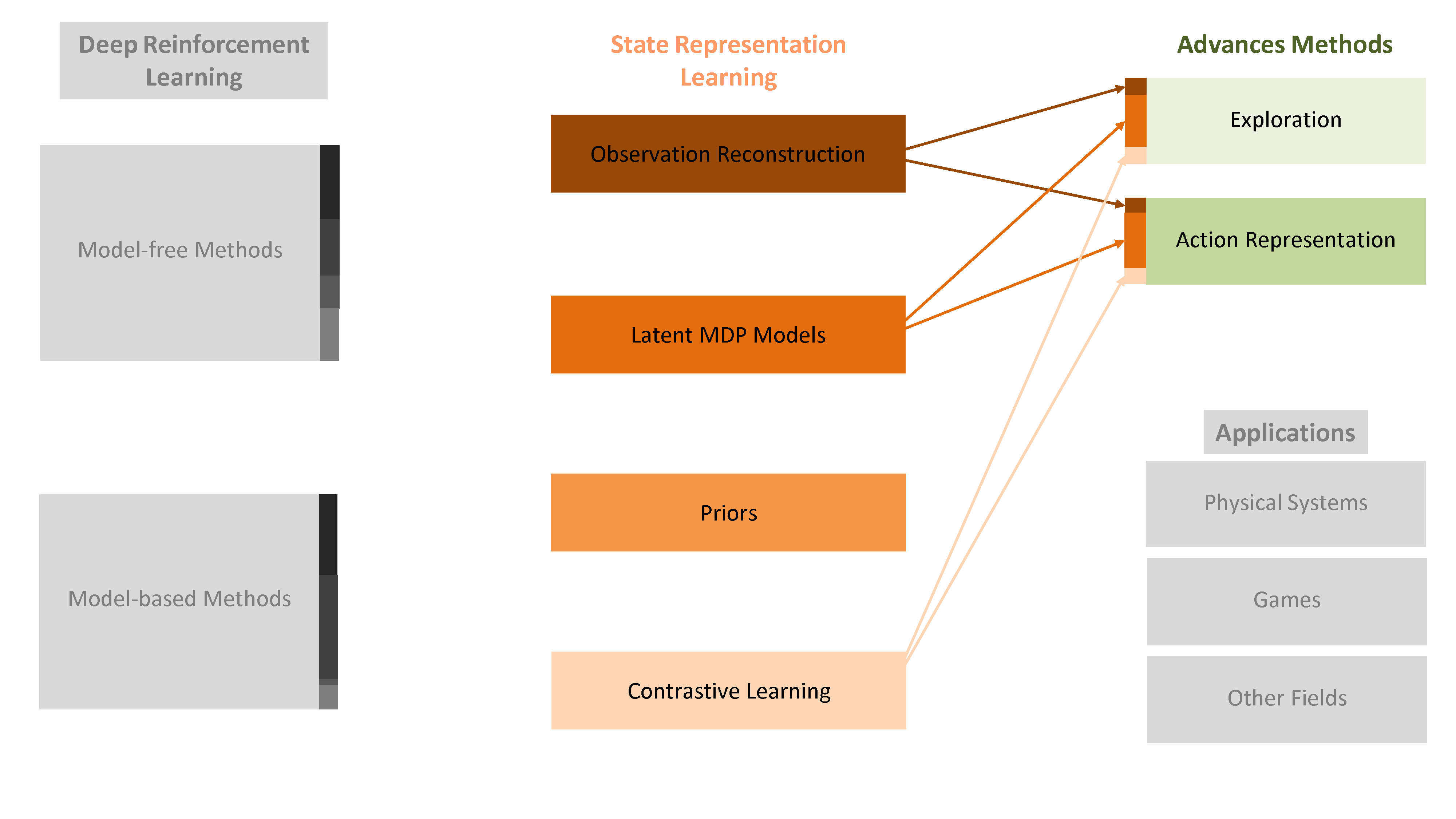
Figure 21: Overview of advanced methods.

5.1 Advanced Methods

We enhance the review by studying two crucial challenges for scaling DRL to complex applications:

• Enhancing exploration skills of the DRL agents by using the latent representations to generate intrinsic rewards.

• Transforming large action spaces in lower-dimensional latent action spaces for easier policy learning.

5.1.1 State Representation for Efficient Exploration in Complex Environments

The exploration-exploitation dilemma is one of the most studied problems in RL. Efficient exploration of the unknown world while exploiting known rewards is especially problematic in large and complex environments where random exploration or heuristics cannot guarantee sufficient coverage of underlying state space. This aspect is even more severe when the state of the environment is not available to the agent, and only high-dimensional observations are fed to the agent. Learning state representations reveal to be a crucial aspect even in the context of better exploration of the world.

Curiosity-driven exploration [131, 132] founds its success in the concept of rewarding the agent for exploring unexplored areas of the world. Unexplored areas are areas without or with limited samples, therefore hard to predict using, for example, forward models. By rewarding the agent with a scalar value proportional to the prediction error, we promote to visit uncertain states more often and enhance the agent’s exploration skills.

Despite the plethora of work on this topic [133], in this section, we focus on a curiosity-driven exploration through learning state representations and latent MDP models to highlight further the versatility of SRL and its benefits in many aspects of DRL. Again SRl and the process of encoding observations to a low dimensional space by maintaining the relevant information for exploring is of crucial importance here.

One of the first works combining learned state representations and latent MDP models to generate curiosity rewards is [134], where an encoder trained by an inverse model and a forward model was used to reduce the dimensionality of the observations. The inverse model is used to focus the learning of features that are controllable by the agent and, therefore, more interesting for exploration. The latent forward model and the embeddings of the observations are used to compute the prediction error that was summed to the reward to promote exploration. However, this method presented several limitations that were highlighted in [135]. The major one arises when the environment dynamic is stochastic. The curiosity-driven agent, as it is, could not distinguish uncertainties due to the lack of data from uncertainties due to the stochasticity of the environment dynamics. Therefore the agent was subjected to learning policies that exploited the stochasticity of the environment without any exploratory meaning. Improvements to curiosity-driven exploration to limit the problem of the stochasticity of the environment were proposed by[136] where an ensemble of latent forward models was used to make N independent prediction-error terms. The curiosity bonus was then computed by looking at the variance of the error terms as a mean of exploiting disagreement of the models.

Exploration can also be promoted if the agent learns to avoid terminal states that the actions cannot reverse. With this idea in mind, the authors in [137] developed an approach for intelligent exploration that penalized visiting irreversible states. Randomly initialized AEs can also generate exploration bonuses for aiding the visit of different features of the latent state space [138].

Novelty can be defined not only by prediction error but also in terms of how distant a state is from other visited states. This idea was exploited by [139] with the method named episodic curiosity. First, observations were embedded in the latent state space. Then each embedding was compared with the embeddings of novel states, stored in the so-called reachability buffer, to generate a score depending on how far the embedding was from the others in the buffer. If the score was above a certain threshold, i.e. the observation was deemed novel, the observation was added to the reachability buffer. The score was used as a curiosity bonus rewarding the agent for visiting states far from the set of known ones. A similar concept is used by [140], where the curiosity bonus was defined by looking at the latent states’ K-Nearest Neighbours (KNN) to reward visiting states with high KNN scores. States with high KNN scores belonged to areas with more exploratory potential. Closely related, we found the work of [141], where an inverse model aided the learning of the latent states used for computing the KNN score to focus on controllable features, the work of [142] where a contrastive loss was used instead of the inverse model, and the work of [143] that, differently from the other approaches, simultaneously learned a state representation that was directly used by the policy and to generate the exploration bonus.

Eventually, we find the methods keeping track of the visiting count of each state and rewarding exploration strategies achieving uniform coverage [144, 145, 146]. However, these methods struggle in large discrete and continuous state spaces where complicated and expensive density models have to be learned and updated during the exploration process.

5.1.2 Learning Action Representations

Reducing the dimensionality of the observations by encoding them in a lower-dimensional latent state space is a powerful and crucial tool for sample-efficient DRL. In this section, we argue that the same mechanism of encoding can be used for the agent’s actions. While many works have only focused on learning state representations, only a few have focused on learning action representations or jointly learning state and action representations. This section reviews the methods relying on action (and state-action) representations.

One of the first examples is the work of [147] in the context of Natural Language Processing. The goal was to train a DQN agent that, by looking at a sentence, i.e. the state, could predict the sentence that would follow correctly. State and actions are recurrently and independently encoded, and their embeddings, i.e. the state and the action representations, were fed to the Q-network to estimate the Q-value. Learning the Q-value in the latent state-action space proved to be the critical ingredient for outperforming other approaches in the literature.

Large and discrete action spaces are traditionally a challenge for DRL algorithms as it is hard to properly explore the action space. However, one could think of embedding the action space in continuous latent spaces to exploit similarities among actions and allow generalization. Despite different effects, actions with similar effects on the states could be mapped together in the latent action space, making learning the value function and the policy more accessible. In this context, we find the work of [148] that, given an action embedding, computed the K closest actions via KNN, and then evaluated the Q-value of those actions only. This approach efficiently saved evaluations of the Q-value, making the DRL algorithm efficient for large action spaces. Another way to learn action embeddings was proposed by [149]. The authors introduced a variant of an inverse model with a bottleneck. Two consecutive states were used as inputs to an inverse model to predict the latent action between two states. Then, the latent action was fed to a decoder network mapping the latent action to the original action space. A continuous latent policy was efficiently trained to map states to latent actions.

State representation and action representations were combined by [150] using similar principles to [149] with the difference of using a forward model instead of an inverse one. Again embedding states and actions proved to be a powerful way to achieve sample efficiency in DRL, especially in the case of large discrete action spaces where embedding the actions added structures and exploited their similarities. In the same line of thought, the authors of [52] proposed a framework for jointly learning state and action representations from high-dimensional observations by relying on the MDP homomorphism metrics for guaranteeing optimality and equivalence of the latent policy mapping latent state to latent actions and the overall policy from observations to actions.

A similar architecture to [150] was proposed by [151], but, similarly to [147], the action representation was learned from a sequence of actions and not from a single one. Moreover, state and action representations are enforced to be Gaussian distributions using a KL-divergence loss. Because sequences of actions were mapped to a latent action vector, decoding this vector back to a sequence of actions was an ill-posed inverse problem requiring regularization and the complete pre-training of the action encoder.

5.1.3 Discussion

In this section, we aim at briefly summarizing a key aspect of each category of methods:

• In particular, while additional objectives are very often used in this context, especially in online exploration, we notice that forward, and inverse models are used to extract the set of epistemically uncertain yet controllable features.

• Similarly to model-based DRL, the exploration via forward models requires precise quantification and discrimination of aleatoric and epistemic uncertainties. Deepening the connection between uncertainty quantification, SRL and learning latent dynamical models is an important aspect to address for further progress.

• Combining the learning of state and action representations from high-dimensional observation has been proposed only in [151, 52]. These approaches may open the door to more sample-efficient DRL algorithms combined with temporal abstractions of action and states.

In Table 4, we summarize how the contributions presented utilize the SRL methods.

Table 4: Which SRL methods are used by each contribution?

Method ($\rightarrow$) Contribution ($\downarrow$)	PCA	AE	VAE	FW	RW	IN	MDP H	BM	PR	CL	Other Objectives
[134]
[135]
[136]
[137]
[139]
[140]
[141]
[142]
[143]
[138]
[144]
[145]
[146]
[147]
[148]
[149]
[150]
[151]
[52]

In Figure 21, we show the use of the SRL methods in exploration and action representation. In both cases, the latent MDP models are the most often employed methods and the priors are never used.

5.2 Applications

After an in-depth presentation of the basic approaches, methods and advanced methods, we focus on the most relevant applications of SRL (see Figure 22). State estimation is one of the most well-studied problems in dynamical systems evolving over time. Predicting such systems’ natural and controlled evolution is crucial when we talk about physical systems, such as robotics and fluid dynamics, games, e.g. chess or Atari, and other fields such as health and finance.

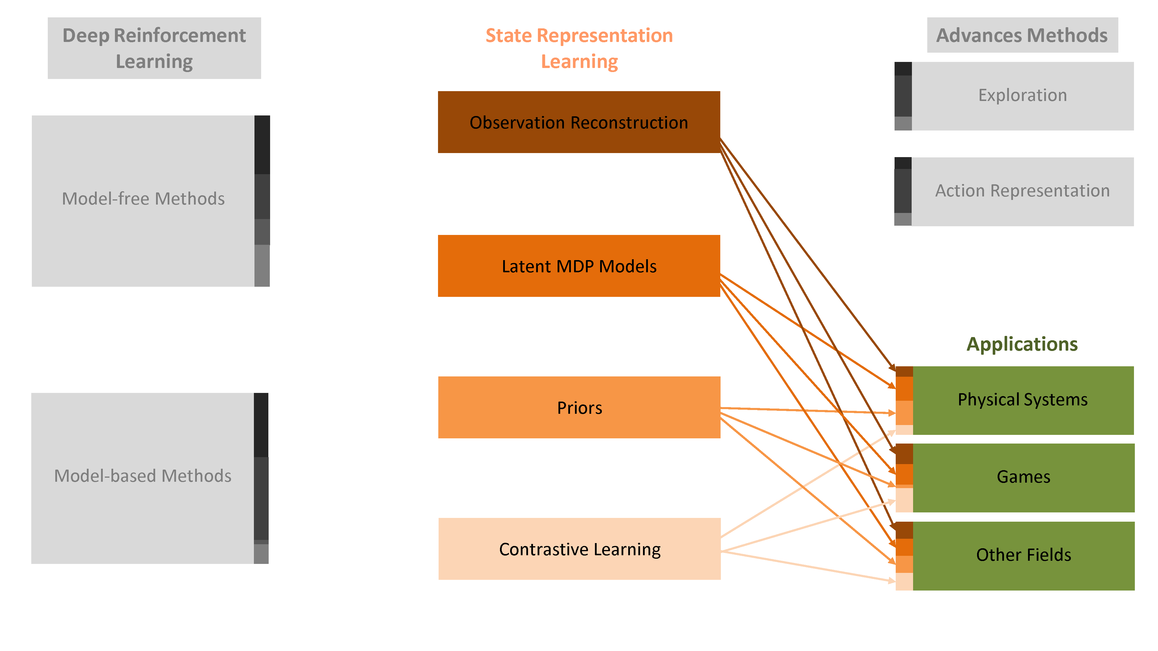
Figure 22: Overview of the applications.

5.2.1 Physical Systems

Physical systems often present a crucial challenge: real-world interaction. The interaction with the real world, and the consequent need for learning from limited data, is possibly the most significant obstacle DRL-based control systems have to overcome. In the context of physical systems, robotics is one of the most researched application domains due to the potential societal impacts of autonomous robots and the possibility of studying how to deal with the real world and tackle the problem of learning from limited samples.

Simulators are often used as a proxy for the real world. However, the simulation-to-reality gap often hinders the direct transfer of the learned behaviours to the real world [152]. SRL plays an important role here as well. Dimensionality reduction makes the low-dimensional state representations and the policies learned, given such representations, more robust to noise, visual distractors, and discrepancies between the simulator and the real world compared to DRL algorithms learning directly from high-dimensional measurements. Moreover, due to the higher sample efficiency of the DRL algorithm, it is possible to fine-tune the performance with real-world samples in some cases.

Alternatively, one could think of training the algorithms directly in the real world. While model-free approaches are predominant with simulators, model-based approaches become more appealing when learning directly in the real world. Therefore, learning accurate and reduced-order latent models from measurements is crucial. Again, sample efficiency and robustness are the two essential concepts that must be considered.

The literature proposed a wide variety of robotics applications from mobile robot navigation, dexterous manipulation with robot arms, autonomous driving, and continuous control In the context of continuous control with DRL, especially in recent years, fluid dynamics has gathered more attention [153]. While traditionally, fluid dynamics has focused only on model-order reduction and state estimation. SRL principles have yet to be exploited in this field, but they can be crucial for systems without known physical models.

5.2.2 Games

Games such as chess, Go, Atari and Montezuma’s Revenge are other examples of successful application of SRL and DRL. While sample efficiency might not appear critical due to the lack of real-world interaction, solving games with long-term dependencies, multiple levels of difficulty, requiring complex exploration policies, against or in collaboration with multiple players requires unobtainable amounts of data. Therefore, learning good and general state representations and latent models can allow the development of new approaches and more advanced solutions to, for example, efficient exploration or credit assignment.

Unlike physical systems, where continuous action spaces are often preferred for the smoothness of the control laws, games present discrete action spaces spanning from simple north-south-west-east movements on a grid to more complex actions such as grabbing objects opening doors and moving different chess pieces.

5.2.3 Other fields

DRL has become increasingly popular in many applications in different fields in recent years. However, SRL methods remain understudied. Here, we show how the problem-specific challenges of each field can enormously benefit from SRL methods.

The first example is economics. Decision-making problems such as the stock market, portfolio management and allocation of capital, online services and recommendations systems can all be tackled with DRL [154]. Improving information compression, quantifying uncertainties in the measured variables over wide windows of time, and providing interpretable results are some problems the SRL methods could potentially solve.

Secondly, the health domain [155] has recently shifted its focus towards dynamic treatment regimes with long-term effects for chronic disease, automated medical diagnoses, and health resource scheduling and allocation, e.g. time slots, nursing resources, and diagnostic devices. Many challenges arise in this field, such as sample efficiency due to the limited data, state-action spaces engineering due to multiple high-dimensional measurements over long time windows and potentially coming from different devices, interpretability of the decisions and the learned latent variables, development of patient-specific models, dealing with uncertainties, exploration of new treatment regimes, and the integration of prior knowledge. These challenges perfectly fit the scope of SRL methods, and SRL can open new frontiers in health research.

DRL has also invaded domains such as the Internet of Things (IoT) and communication networks [156] for solving power control and power management, reducing latency and traffic load problems, and cloud computing, smart grid, and resource allocation. With many users involved, the key challenges include dealing with multi-agent systems and encoding partial information over time.

Natural Language Process presents problems that DRL has started to solve, such as language understanding, text generation, machine translation and conversational systems [157]. The proper encoding and representation of sentences and sounds and the generalization to new speakers are crucial for decision making. SRL may be again an essential element for further progress.

Eventually, we find the field of Explainable AI (ExAI) [158, 159]. ExAI aims to open the black box and, in DRL, understand the agent’s behaviour. SRL can be seen as a way to simplify the problem of decision-making by separating feature extraction and policy learning by identifying the low-dimensional set of important variables for control. These SRL goals align with ExAI, and further research should be conducted to strengthen this connection.

5.3 Summary

In Figure 22, we show the use of the SRL methods for the different groups of applications. In particular, we highlight:

• latent models, and priors play a crucial role for physical systems where prediction of the dynamics of the world is often as important as the learning of the policy. When dealing with physical interaction with the world, model-based DRL is preferable to model-free.

• model-free DRL is often preferred for games, and contrastive losses are often employed next to DRL algorithm loss (e.g. reward maximization) to help the learning of good state representations.

• in other field, SRL principles have yet to be studied and exploited. Therefore, each of the four SRL methods has the potential to bring important contribution to the different fields.

6 Evaluation and Benchmark

6.1 Evaluation Metrics

Evaluating the learned representations is crucial for assessing and comparing new approaches, especially in DRL, where many results come from empirical evaluations. We can identify three major ways of evaluating state representations:

• Reward over training and testing.

• Structural metrics.

• Qualitative metrics.

6.1.1 Reward Over Training

The reward over training and testing is the most used of the metrics. The quality of the different learned representations is indirectly compared using the training speed of the learned policy and its robustness when tested. The policy can be learned jointly with the representation or after the representation is entirely learned. The performance of the agent is ultimately the critical metric in DRL. However, it is usually computational expensive to train multiple agents, the performance is heavily dependent on the choice of the DRL algorithm and its hyperparameters, making it difficult to disentangle the benefits of the learned representation from the overall increment of the cumulative rewards.

6.1.2 Structural Metrics

An alternative and appealing way of assessing the learned representations’ quality is using the so-called structural metrics. Structural metrics are all the metrics evaluating the properties of learned representations independently of the performance of the DRL agent. An example is a relation between the learned states and the actual states of the environment. Common structural metrics are:

• Ground Truth Correlation (GTC) [161] measuring the correlation between the learned states and the true environment states.

• K-Nearest Neighbour (K-NN) [161] measuring the distance between K neighbours of latent states and K neighbours of true states.

• Linear Reconstruction Error (LRE) [29] measuring the disentangle of the state features by linearly mapping them to their respective true state value.

• Validation Decoder [15] measuring if the latent states can be used to reconstruct the observations without disambiguities.

• Ground Truth Error (GTE) [162] measuring the error to the ground truth with Euclidean or geodesic distance.

• Normalization Independent Embedding Quality Assessment (NIEQA) [163] measures the quality of the latent manifold in terms of preservation of the true underlying structure.

• Feature predictiveness [64] measuring how many of the features learned by the encoder are used by the forward model for predicting the future states.

• Hits at rank K [31] measuring if the predicted latent state belongs to the K-NN of the true encoded observation.

6.1.3 Qualitative Metrics

Eventually, qualitative evaluations are often provided by the authors of the papers, especially when the representation is attributable to a lower-dimensional domain, e.g. robot control, where the features can be directly related to physical quantities, such as positions and velocities. Visualization of latent representations is crucial for interpretability. Because in most cases, it is preferred to keep the dimension of the latent representation higher than the actual state space, usually PCA or t-distributed Stochastic Neighbour Embedding (t-SNE) [164] are used to project, linearly and non-linearly, respectively, the latent state variables into a visualizable space, i.e. 2D or 3D, that can be plotted. However, complex problems cannot often be reduced to plottable dimensions. Therefore, their interpretability remains an open problem in the literature.

6.2 Benchmarks

SRL algorithms are usually evaluated using the same environments built for DRL. Their domains span from the Atari games to continuous control tasks such as pendulum and cheetah. Below, we list the most used platforms:

• Atari Learning Environment [114] providing an RL interface to the Atari games with the possibility of playing them from pixels. The Atari games offer the possibility of testing discrete state and action spaces algorithms and present several challenges to the algorithms, such as partial observability, long-term exploration, and reward sparsity.

• DeepMind Control Suite [165] including a vast range of continuous control tasks such as pendulum, cheetah, and humanoid. Continuous control tasks require the algorithms to deal with continuous state and action spaces, multiple degrees of freedom, and partial observability when played from pixels. The physics is simulated by Mujoco [166].

• DeepMind Lab [167] introducing a first-person 3D environment for testing the navigation, exploration, and generalization skills of the agents.

• SRL-Toolbox [161] offering a complete package with many of the early SRL approaches from the literature, evaluation functions, and a set of testing environments, smaller if compared to the other platforms.

• OpenAI-Gym [168] collecting a wide variety of RL environments, spanning from the Atari games to continuous control and robotics problems.

7 Discussion

In Figure 23, we provide a graphical overview of the SRL methods in model-free and model-based DRL and their role in advanced methods and applications.

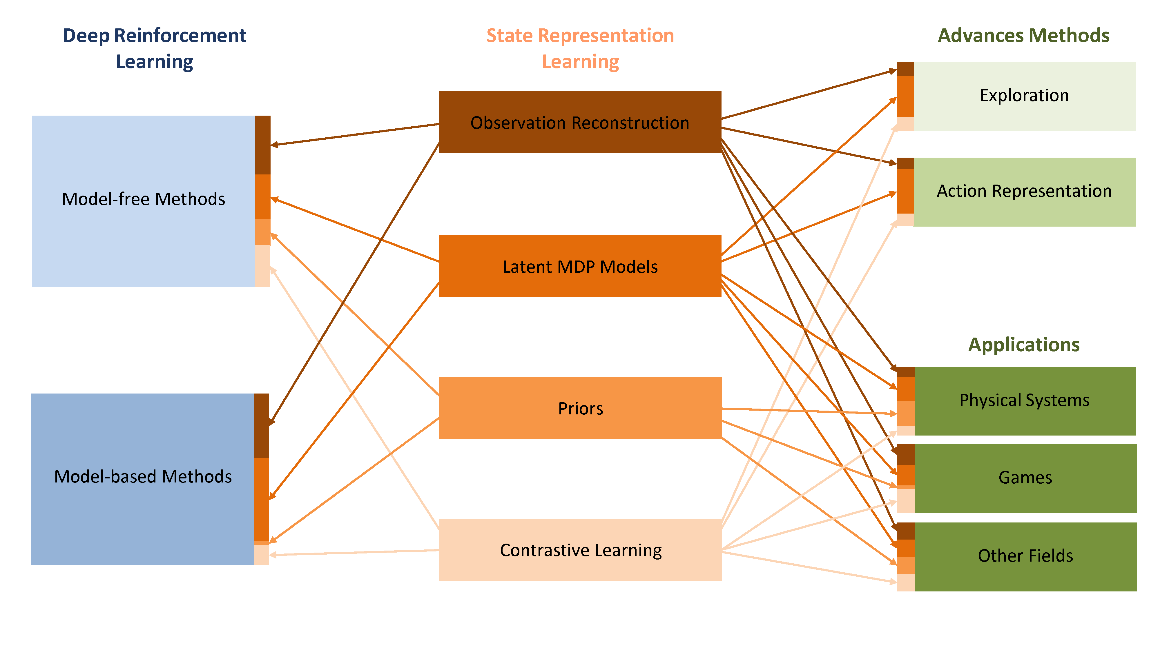
Figure 23: The big picture.

Eventually, we discuss two final aspects: (i) open challenges and (ii) future directions.

7.1 Open Challenges and Future Directions

DRL and SRL are two quickly-evolving fields, and here we summarize the most exciting future directions. From our review of the literature, we have identified several aspects that are currently understudied in the field:

• the incorporation of inductive biased and prior knowledge in the neural network architectures using the tools provided by Geometric Deep Learning [129],

• the proper quantification of uncertainties in the latent variables, observations, and MDP dynamics,

• the learning of general representations using the Meta-Learning paradigm [169], and

• the evaluation and comparison of the approaches and the interpretability and explainability of the latent representations.

7.1.1 Incorporation of Inductive Biases

In the last decade, DL has solved many high-dimensional problems considered beyond reach by developing increasingly complex architectures with a continuously-growing number of parameters and requiring more data.

When scaling to larger problems, simply increasing the model complexity and the size of the training set do not seem viable options. However, many complex problems present low-dimensional structures, symmetries, and geometry deriving from the physical world. Incorporating this knowledge into the neural network architectures and the learned representations is essential for tackling the curse of dimensionality, reducing the number of parameters needed by each model, and improving generalization to unseen data [129]. For example, when learning a latent forward model for a mobile robot, we would like the model to learn invariant features to background changes or noise in the measurements.

The SRL methods described in this review have prepared the ground for incorporating geometry, group theory and symmetries in DRL methods. Exploiting symmetries, structures, and prior knowledge are three critical ingredients for sample efficient SRL and DRL that are yet under-investigated but have shown outstanding potential for future research [170, 171].

7.1.2 Uncertainty Quantification in Unsupervised Representation Learning

Uncertainties may arise from different sources, e.g. the measurement noise or the chaotic dynamics of the system at hand. Quantifying and disentangling these data uncertainties is crucial to the generalization of state representations and latent models. While this problem is primarily studied in supervised learning [172], it is even more complex in unsupervised representation learning in dynamical systems. The goal of understanding and discovering the low-dimensional set of variables describing the evolution of the systems cannot be achieved without proper uncertainty quantification.

In particular, we highlight Deep Kernel Learning [173, 174, 175] as a computationally-efficient approach, scalable to high-dimensional data, for combining the expressive power of neural networks with the uncertainty quantification abilities of Gaussian processes and kernel methods [176].

7.1.3 Meta-Learning General Representations

DRL agents have faced an uncountable amount of different tasks, and this trend is only destined to grow in the future. Learning to adjust the behavior to new problems from limited data is still an open question in DRL research. While the Meta-Learning has been studied in DRL for learning general-purpose policies [177, 178, 179], this paradigm has yet to be exploited for learning general-purpose state and action representations and MDP models. In contrast, with the expensive Meta-DRL from high-dimensional observations, Meta-Learning of representations may provide new ways to tackle the problem of generalization and transfer learning of the learned policy to new tasks and new environments in an efficient sample manner.

7.1.4 Evaluation and Interpretability of the Latent Representations

In Section Evaluation and Benchmark, we discussed different metrics for assessing the quality of the representations, e.g. through the reward over training, structural and qualitative metrics.

However, here we argue that none of these metrics provides the ultimate answer to which method is the best. While the reward over training is the most popular metric, this is subjected to the intrinsic stochasticity of the DRL process, and the results need to be evaluated over multiple runs. The need for multiple runs makes the process extremely computational and resource-intensive for complex environments and high-dimensional observations. On the other side, structural metrics provide a good way of comparing approaches without high-computational demands. However, high metric scores do not necessarily translate into optimal policy results and the highest reward over training. The same holds for qualitative metrics. High human-interpretability of the representations does not necessarily mean optimal behaviors of the agents.

Therefore, we believe that further research must be done to understand what the optimal state representation is, how to learn it, and how to interpret and explain representations and agents’ behaviors.

8 Conclusion

This paper reviewed the most important and newest research trends on unsupervised SRL in DRL. From the literature, we identified four major classes of SRL methods: observation reconstruction, learning of latent MDP models, using priors, and contrastive learning. Moreover, we study how these methods are combined to develop more complex approaches. Eventually, we extended the review to include the advanced methods and applications of SRL.

Unsupervised representation learning has proven to be a crucial element of the best-performing DRL algorithms for improving sample efficiency, robustness, generalization, and interpretability. Despite the progress in the field, many issues remain open for tackling complex real-world problems.

The incorporation of prior knowledge and geometry, the exploitation and learning of symmetries, the quantification of the uncertainties, the generalization to different tasks, and the evaluation and interpretability of the representations are important problems to address in the future.

Appendix A Implementation Details

A.1 Code

In this section, we provide the implementation details for reproducing the results presented in Section Deep Learning for Learning State Representations. The code used for generating the results and the dataset used is publicly available at https://github.com/nicob15/State_Representation_Learning_Methods. The code is constructed using the PyTorch [180].

A.1.1 Pendulum Model

For our experiments, we consider the pendulum described by the following equation:

$$\ddot{\psi}(t)=-\frac{1}{ml}(mg\sin{\psi}(t)+a(t))\,,$$ (35)

where $\psi$ is the angle of the pendulum, $\ddot{\psi}$ is the angular acceleration, $m$ is the mass, $l$ is the length, and $g$ denotes the gravity acceleration.

We assume no access to $\psi$ or its derivatives, and the measurements are RGB images of size $84\times 84\times 3$ obtained through an RGB camera and we utilize frame stacking to allow the network to infer velocity information, making the observations of size $84\times 84\times 6$. The observation are collected by following a random policy for 200 steps with different initial conditions. The training set is composed of 10000 data tuples $(\mathbf{o}_{t},a_{t},\mathbf{o}_{t+1})$, while the test set is composed of 2000 data tuples. Different random seeds are used for collecting training and test sets.

The pendulum environment used for collecting the data tuples is the Pendulum-v1 from Open-Gym [168].

A.1.2 Encoder Architecture

The input observations are two $84\times 84\times 3$ RGB images stacked together. The (deterministic) encoder $\phi_{\text{enc}}$ is composed of 4 convolutional layers with 32 filters per layer. The convolutional filters are of size $(3\times 3)$ and shifted across the images with stride 1 (only the first convolutional layer has stride 2 to quickly reduce the input dimensionality). Batch normalization is also used after the 2nd and 4th convolutional layers. A similar convolutional architecture is used in PlaNet[123] and Dreamer[124]. The output features of the last convolutional layer are flattened and fed to two final fully connected layers of dimensions 256 and 50, respectively, compressing the features to a 50-dimensional latent state vector. Each layer has ELU activations, except the last fully-connected layer with a linear activation.

Analogously, the VAE (stochastic) encoder shares the same architecture with the deterministic encoders but instead of learning the latent state vectors $\mathbf{z}_{t}$, the encoder learns the mean and the covariance of a Gaussian distribution representing the distribution $p(\bm{z}_{t}|\bm{o}_{t})=\mathcal{N}(\bm{\mu}_{t},\bm{\Sigma}_{t})$. Samples $\bm{z}_{t}$ from $p(\bm{z}_{t}|\bm{o}_{t})$ are obtained by reparametrization trick [27].

A.1.3 Decoder Architecture

The decoder $\phi_{\text{dec}}$ is parametrized by an NN composed of a linear fully-connected layer and 4 transpose convolutional layers with 32 filters each. The convolutional filters are of size $(3\times 3)$ and shifted across the images with stride 1 (again, the last convolutional layer has stride 2). Batch normalization is used after the 2nd and 4th convolutional layers, and ELU activations are employed for all the layers except the last one. The output is the observation reconstruction $\hat{\bm{o}}_{t}$.

A.1.4 Latent Models Architectures

The latent models implemented are:

• forward model with input $\bm{z}_{t}$ and $\bm{a}_{t}$ and output $\bm{z}_{t+1}$,

• reward with input $\bm{z}_{t}$ and $\bm{a}_{t}$ or $\bm{z}_{t}$ and output the predicted reward $\hat{r}_{t}$,

• inverse with input $\bm{z}_{t}$ and $\bm{z}_{t+1}$ and output the predicted action $\hat{\bm{a}}_{t}$, and

• action encoder with input $\bm{z}_{t}$ and $\bm{a}_{t}$ and output $\bar{\bm{a}}_{t}$

All these models are composed of an input layer of size dependent on the input data, an hidden layer of size 256, and an output layer again model-dependent.

A.1.5 Hyperparameters of the Experiments

The hyperparameters used in our experiments are reported in Table 5, where for fairness of comparison they are shared among the different methods.

Hyperparameter	Value
learning rate of NN	$3\mathrm{e}-4$
$L^{2}$ regularization coefficient	$1\mathrm{e}{-3}$
$\beta$ (VAE)	$0.5$
$\gamma$ (BM)	$0.99$
number of epochs	$50$
latent state dimension	$50$
latent action dimension	$50$
image dimension	$84\times 84\times 3$
observation dimension	$84\times 84\times 6$
action dimension	1
mass of the pendulum	1
length of the pendulum	1

Table 5: Hyperparameters used in the experiments.

References

- Brunton et al. [2016] Steven L Brunton, Joshua L Proctor, and J Nathan Kutz. Discovering governing equations from data by sparse identification of nonlinear dynamical systems. Proceedings of the national academy of sciences, 113(15):3932–3937, 2016.
- Winston [1984] Patrick Henry Winston. Artificial intelligence. Addison-Wesley Longman Publishing Co., Inc., 1984.
- Mitchell and Mitchell [1997] Tom M Mitchell and Tom M Mitchell. Machine learning, volume 1. McGraw-hill New York, 1997.
- Brunton and Kutz [2022] Steven L Brunton and J Nathan Kutz. Data-driven science and engineering: Machine learning, dynamical systems, and control. Cambridge University Press, 2022.
- Sutton and Barto [1998] R.S. Sutton and A.G. Barto. Reinforcement Learning: An Introduction. IEEE Transactions on Neural Networks, 9(5), 1998. ISSN 1045-9227. doi:10.1109/tnn.1998.712192.
- Puterman [1990] Martin L Puterman. Markov decision processes. Handbooks in operations research and management science, 2:331–434, 1990.
- LeCun et al. [2015] Yann LeCun, Yoshua Bengio, and Geoffrey Hinton. Deep learning. nature, 521(7553):436–444, 2015.
- Mnih et al. [2013] Volodymyr Mnih, Koray Kavukcuoglu, David Silver, Alex Graves, Ioannis Antonoglou, Daan Wierstra, and Martin Riedmiller. Playing atari with deep reinforcement learning. arXiv preprint arXiv:1312.5602, 2013.
- Mnih et al. [2015] Volodymyr Mnih, Koray Kavukcuoglu, David Silver, Andrei A Rusu, Joel Veness, Marc G Bellemare, Alex Graves, Martin Riedmiller, Andreas K Fidjeland, Georg Ostrovski, et al. Human-level control through deep reinforcement learning. nature, 518(7540):529–533, 2015.
- Arulkumaran et al. [2017] Kai Arulkumaran, Marc Peter Deisenroth, Miles Brundage, and Anil Anthony Bharath. Deep reinforcement learning: A brief survey. IEEE Signal Processing Magazine, 34(6):26–38, 2017.
- Bengio et al. [2013] Yoshua Bengio, Aaron Courville, and Pascal Vincent. Representation learning: A review and new perspectives. IEEE Transactions on Pattern Analysis and Machine Intelligence, 35(8), 2013. ISSN 01628828. doi:10.1109/TPAMI.2013.50.
- Böhmer et al. [2015] Wendelin Böhmer, Jost Tobias Springenberg, Joschka Boedecker, Martin Riedmiller, and Klaus Obermayer. Autonomous Learning of State Representations for Control: An Emerging Field Aims to Autonomously Learn State Representations for Reinforcement Learning Agents from Their Real-World Sensor Observations. KI - Kunstliche Intelligenz, 29(4), 2015. ISSN 16101987. doi:10.1007/s13218-015-0356-1.
- Lesort et al. [2018] Timothée Lesort, Natalia Díaz-Rodríguez, Jean-François Goudou, and David Filliat. State Representation Learning for Control: An Overview. 2018.
- Achille and Soatto [2017] Alessandro Achille and Stefano Soatto. A Separation Principle for Control in the Age of Deep Learning. 2017.
- Morik et al. [2019] Marco Morik, Divyam Rastogi, Rico Jonschkowski, and Oliver Brock. State representation learning with robotic priors for partially observable environments. In 2019 IEEE/RSJ International Conference on Intelligent Robots and Systems (IROS), pages 6693–6699. IEEE, 2019.
- Jonschkowski and Brock [2015] Rico Jonschkowski and Oliver Brock. Learning state representations with robotic priors. Autonomous Robots, 39(3):407–428, 2015.
- Sanders et al. [2020] Jaron Sanders, Alexandre Proutière, and Se-Young Yun. Clustering in block markov chains. The Annals of Statistics, 48(6):3488–3512, 2020.
- Du et al. [2019] Simon Du, Akshay Krishnamurthy, Nan Jiang, Alekh Agarwal, Miroslav Dudik, and John Langford. Provably efficient rl with rich observations via latent state decoding. In International Conference on Machine Learning, pages 1665–1674. PMLR, 2019.
- Goodfellow et al. [2016] Ian Goodfellow, Yoshua Bengio, and Aaron Courville. Deep learning. MIT press, 2016.
- Botteghi [2021] Nicolò Botteghi. Robotics deep reinforcement learning with loose prior knowledge. University of Twente, 2021.
- Hornik et al. [1989] Kurt Hornik, Maxwell Stinchcombe, and Halbert White. Multilayer feedforward networks are universal approximators. Neural networks, 2(5):359–366, 1989.
- LeCun et al. [1995] Yann LeCun, Yoshua Bengio, et al. Convolutional networks for images, speech, and time series. The handbook of brain theory and neural networks, 3361(10):1995, 1995.
- Pineda [1987] Fernando J Pineda. Generalization of back-propagation to recurrent neural networks. Physical review letters, 59(19):2229, 1987.
- Graves [2012] Alex Graves. Supervised sequence labelling. In Supervised sequence labelling with recurrent neural networks, pages 5–13. Springer, 2012.
- Wold et al. [1987] Svante Wold, Kim Esbensen, and Paul Geladi. Principal component analysis. Chemometrics and intelligent laboratory systems, 2(1-3):37–52, 1987.
- Lecun [1987] Yann Lecun. Phd thesis: Modeles connexionnistes de l’apprentissage (connectionist learning models). 1987.
- Kingma and Welling [2014] Diederik P Kingma and Max Welling. Stochastic gradient vb and the variational auto-encoder. In Second International Conference on Learning Representations, ICLR, volume 19, page 121, 2014.
- Jonschkowski and Brock [2014] Rico Jonschkowski and Oliver Brock. State representation learning in robotics: Using prior knowledge about physical interaction. In Robotics: Science and Systems, 2014.
- Chopra et al. [2005] Sumit Chopra, Raia Hadsell, and Yann LeCun. Learning a similarity metric discriminatively, with application to face verification. In 2005 IEEE Computer Society Conference on Computer Vision and Pattern Recognition (CVPR’05), volume 1, pages 539–546. IEEE, 2005.
- Higgins et al. [2016] Irina Higgins, Loic Matthey, Arka Pal, Christopher Burgess, Xavier Glorot, Matthew Botvinick, Shakir Mohamed, and Alexander Lerchner. beta-vae: Learning basic visual concepts with a constrained variational framework. 2016.
- Kipf et al. [2019] Thomas Kipf, Elise van der Pol, and Max Welling. Contrastive learning of structured world models. In International Conference on Learning Representations, 2019.
- François-Lavet et al. [2019] Vincent François-Lavet, Yoshua Bengio, Doina Precup, and Joelle Pineau. Combined reinforcement learning via abstract representations. In Proceedings of the AAAI Conference on Artificial Intelligence, volume 33, pages 3582–3589, 2019.
- van der Pol et al. [2020a] Elise van der Pol, Thomas Kipf, Frans A Oliehoek, and Max Welling. Plannable approximations to mdp homomorphisms: Equivariance under actions. In Proceedings of the 19th International Conference on Autonomous Agents and MultiAgent Systems, pages 1431–1439, 2020a.
- Goroshin et al. [2015] Ross Goroshin, Michael Mathieu, and Yann Lecun. Learning to linearize under uncertainty. In Advances in Neural Information Processing Systems, volume 2015-Janua, 2015.
- Van Hoof et al. [2016] Herke Van Hoof, Nutan Chen, Maximilian Karl, Patrick van der Smagt, and Jan Peters. Stable reinforcement learning with autoencoders for tactile and visual data. In 2016 IEEE/RSJ international conference on intelligent robots and systems (IROS), pages 3928–3934. IEEE, 2016.
- Agrawal et al. [2016] Pulkit Agrawal, Ashvin Nair, Pieter Abbeel, Jitendra Malik, and Sergey Levine. Learning to poke by poking: Experiential learning of intuitive physics. Advances in Neural Information Processing Systems, pages 5074–5082, 2016. ISSN 10495258.
- Gelada et al. [2019] Carles Gelada, Saurabh Kumar, Jacob Buckman, Ofir Nachum, and Marc G Bellemare. Deepmdp: Learning continuous latent space models for representation learning. In International Conference on Machine Learning, pages 2170–2179. PMLR, 2019.
- Ravindran and Barto [2002] Balaraman Ravindran and Andrew G Barto. Model minimization in hierarchical reinforcement learning. In International Symposium on Abstraction, Reformulation, and Approximation, pages 196–211. Springer, 2002.
- Ravindran and Barto [2004] Balaraman Ravindran and Andrew G Barto. Approximate homomorphisms: A framework for non-exact minimization in markov decision processes. 2004.
- Givan et al. [2003] Robert Givan, Thomas Dean, and Matthew Greig. Equivalence notions and model minimization in markov decision processes. Artificial Intelligence, 147(1-2):163–223, 2003.
- Ferns et al. [2004] Norm Ferns, Prakash Panangaden, and Doina Precup. Metrics for finite markov decision processes. In UAI, volume 4, pages 162–169, 2004.
- Taylor et al. [2008] Jonathan Taylor, Doina Precup, and Prakash Panagaden. Bounding performance loss in approximate mdp homomorphisms. Advances in Neural Information Processing Systems, 21:1649–1656, 2008.
- Zhang et al. [2020] Amy Zhang, Rowan McAllister, Roberto Calandra, Yarin Gal, and Sergey Levine. Learning Invariant Representations for Reinforcement Learning without Reconstruction. jun 2020. ISSN 2331-8422. URL http://arxiv.org/abs/2006.10742.
- Raissi et al. [2019] Maziar Raissi, Paris Perdikaris, and George E Karniadakis. Physics-informed neural networks: A deep learning framework for solving forward and inverse problems involving nonlinear partial differential equations. Journal of Computational physics, 378:686–707, 2019.
- Lesort et al. [2019] Timothée Lesort, Mathieu Seurin, Xinrui Li, Natalia Díaz-Rodríguez, and David Filliat. Deep unsupervised state representation learning with robotic priors: a robustness analysis. In 2019 International Joint Conference on Neural Networks (IJCNN), pages 1–8. IEEE, 2019.
- Laskin et al. [2020] Michael Laskin, Aravind Srinivas, and Pieter Abbeel. Curl: Contrastive unsupervised representations for reinforcement learning. In International Conference on Machine Learning, pages 5639–5650. PMLR, 2020.
- Oord et al. [2018] Aaron van den Oord, Yazhe Li, and Oriol Vinyals. Representation learning with contrastive predictive coding. arXiv preprint arXiv:1807.03748, 2018.
- Chen et al. [2020] Ting Chen, Simon Kornblith, Mohammad Norouzi, and Geoffrey Hinton. A simple framework for contrastive learning of visual representations. In International conference on machine learning, pages 1597–1607. PMLR, 2020.
- Henaff [2020] Olivier Henaff. Data-efficient image recognition with contrastive predictive coding. In International Conference on Machine Learning, pages 4182–4192. PMLR, 2020.
- Stooke et al. [2021] Adam Stooke, Kimin Lee, Pieter Abbeel, and Michael Laskin. Decoupling representation learning from reinforcement learning. In International Conference on Machine Learning, pages 9870–9879. PMLR, 2021.
- You et al. [2022] Bang You, Oleg Arenz, Youping Chen, and Jan Peters. Integrating contrastive learning with dynamic models for reinforcement learning from images. Neurocomputing, 2022.
- Botteghi et al. [2021a] Nicolò Botteghi, Mannes Poel, Beril Sirmacek, and Christoph Brune. Low-dimensional state and action representation learning with mdp homomorphism metrics. arXiv preprint arXiv:2107.01677, 2021a.
- Botteghi et al. [2021b] Nicolò Botteghi, Khaled Alaa, Mannes Poel, Beril Sirmacek, Christoph Brune, Abeje Mersha, and Stefano Stramigioli. Low dimensional state representation learning with robotics priors in continuous action spaces. In IEEE/RSJ International Conference on Intelligent Robots and Systems (IROS), pages 190–197. IEEE, 2021b.
- Curran et al. [2015] William Curran, Tim Brys, Matthew Taylor, and William Smart. Using pca to efficiently represent state spaces, 2015.
- Parisi et al. [2017] Simone Parisi, Simon Ramstedt, and Jan Peters. Goal-driven dimensionality reduction for reinforcement learning. In 2017 IEEE/RSJ International Conference on Intelligent Robots and Systems (IROS), pages 4634–4639. IEEE, 2017.
- Lange and Riedmiller [2010] Sascha Lange and Martin Riedmiller. Deep auto-encoder neural networks in reinforcement learning. In The 2010 International Joint Conference on Neural Networks (IJCNN), pages 1–8. IEEE, 2010.
- Mattner et al. [2012] Jan Mattner, Sascha Lange, and Martin Riedmiller. Learn to swing up and balance a real pole based on raw visual input data. In International Conference on Neural Information Processing, pages 126–133. Springer, 2012.
- Alvernaz and Togelius [2017] Samuel Alvernaz and Julian Togelius. Autoencoder-augmented neuroevolution for visual doom playing. In 2017 IEEE Conference on Computational Intelligence and Games, CIG 2017, 2017. doi:10.1109/CIG.2017.8080408.
- Kempka et al. [2016] Michał Kempka, Marek Wydmuch, Grzegorz Runc, Jakub Toczek, and Wojciech Jaśkowski. Vizdoom: A doom-based ai research platform for visual reinforcement learning. In 2016 IEEE conference on computational intelligence and games (CIG), pages 1–8. IEEE, 2016.
- Higgins et al. [2017] Irina Higgins, Arka Pal, Andrei Rusu, Loie Matthey, Christopher Burgess, Alexander Pritzel, Matthew Botvinick, Charles Blundell, and Lexander Lerchner. DARLA: Improving zero-shot transfer in reinforcement learning. In 34th International Conference on Machine Learning, ICML 2017, volume 3, 2017.
- Vincent et al. [2008] Pascal Vincent, Hugo Larochelle, Yoshua Bengio, and Pierre-Antoine Manzagol. Extracting and composing robust features with denoising autoencoders. In Proceedings of the 25th international conference on Machine learning, pages 1096–1103, 2008.
- Caselles-Dupré et al. [2018] Hugo Caselles-Dupré, Michael Garcia-Ortiz, and David Filliat. Continual state representation learning for reinforcement learning using generative replay. arXiv preprint arXiv:1810.03880, 2018.
- Nair et al. [2018] Ashvin Nair, Vitchyr Pong, Murtaza Dalal, Shikhar Bahl, Steven Lin, and Sergey Levine. Visual Reinforcement Learning with Imagined Goals. jul 2018. URL http://arxiv.org/abs/1807.04742.
- Finn et al. [2016] Chelsea Finn, Xin Yu Tan, Yan Duan, Trevor Darrell, Sergey Levine, and Pieter Abbeel. Deep spatial autoencoders for visuomotor learning. In 2016 IEEE International Conference on Robotics and Automation (ICRA), pages 512–519. IEEE, 2016.
- Caselles-Dupré et al. [2019] Hugo Caselles-Dupré, Michael Garcia Ortiz, and David Filliat. Symmetry-based disentangled representation learning requires interaction with environments. Advances in Neural Information Processing Systems, 32, 2019.
- Raffin et al. [2019] Antonin Raffin, Ashley Hill, René Traoré, Timothée Lesort, Natalia Díaz-Rodríguez, and David Filliat. Decoupling feature extraction from policy learning: assessing benefits of state representation learning in goal based robotics. arXiv preprint arXiv:1901.08651, 2019.
- Kim et al. [2021a] Taewon Kim, Yeseong Park, Youngbin Park, Sang Hyoung Lee, and Il Hong Suh. Acceleration of actor-critic deep reinforcement learning for visual grasping by state representation learning based on a preprocessed input image. In 2021 IEEE/RSJ International Conference on Intelligent Robots and Systems (IROS), pages 198–205. IEEE, 2021a.
- Rafailov et al. [2021] Rafael Rafailov, Tianhe Yu, Aravind Rajeswaran, and Chelsea Finn. Offline reinforcement learning from images with latent space models. In Learning for Dynamics and Control, pages 1154–1168. PMLR, 2021.
- Tennenholtz et al. [2021] Guy Tennenholtz, Nir Baram, and Shie Mannor. Gelato: Geometrically enriched latent model for offline reinforcement learning. arXiv preprint arXiv:2102.11327, 2021.
- Shang and Ryoo [2021] Jinghuan Shang and Michael S Ryoo. Self-supervised disentangled representation learning for third-person imitation learning. In 2021 IEEE/RSJ International Conference on Intelligent Robots and Systems (IROS), pages 214–221. IEEE, 2021.
- De Bruin et al. [2018] Tim De Bruin, Jens Kober, Karl Tuyls, and Robert Babuška. Integrating state representation learning into deep reinforcement learning. IEEE Robotics and Automation Letters, 3(3):1394–1401, 2018.
- van Hasselt et al. [2015] Hado van Hasselt, Arthur Guez, and David Silver. Deep reinforcement learning with double q-learning, 2015.
- Yarats et al. [2021a] Denis Yarats, Amy Zhang, Ilya Kostrikov, Brandon Amos, Joelle Pineau, and Rob Fergus. Improving sample efficiency in model-free reinforcement learning from images. In Proceedings of the AAAI Conference on Artificial Intelligence, volume 35, pages 10674–10681, 2021a.
- Ghosh et al. [2019] Partha Ghosh, Mehdi SM Sajjadi, Antonio Vergari, Michael Black, and Bernhard Schölkopf. From variational to deterministic autoencoders. arXiv preprint arXiv:1903.12436, 2019.
- Haarnoja et al. [2018] Tuomas Haarnoja, Aurick Zhou, Pieter Abbeel, and Sergey Levine. Soft actor-critic: Off-policy maximum entropy deep reinforcement learning with a stochastic actor. In International conference on machine learning, pages 1861–1870. PMLR, 2018.
- Lee et al. [2020a] Alex X Lee, Anusha Nagabandi, Pieter Abbeel, and Sergey Levine. Stochastic latent actor-critic: Deep reinforcement learning with a latent variable model. Advances in Neural Information Processing Systems, 33:741–752, 2020a.
- Papoudakis et al. [2021] Georgios Papoudakis, Filippos Christianos, and Stefano Albrecht. Agent modelling under partial observability for deep reinforcement learning. Advances in Neural Information Processing Systems, 34, 2021.
- Mnih et al. [2016] Volodymyr Mnih, Adria Puigdomenech Badia, Mehdi Mirza, Alex Graves, Timothy Lillicrap, Tim Harley, David Silver, and Koray Kavukcuoglu. Asynchronous methods for deep reinforcement learning. In International conference on machine learning, pages 1928–1937. PMLR, 2016.
- Thomas et al. [2017] Valentin Thomas, Jules Pondard, Emmanuel Bengio, Marc Sarfati, Philippe Beaudoin, Marie-Jean Meurs, Joelle Pineau, Doina Precup, and Yoshua Bengio. Independently Controllable Factors. aug 2017. URL http://arxiv.org/abs/1708.01289.
- Bellemare et al. [2017] Marc G Bellemare, Will Dabney, and Rémi Munos. A distributional perspective on reinforcement learning. In International Conference on Machine Learning, pages 449–458. PMLR, 2017.
- Castro [2020] Pablo Samuel Castro. Scalable methods for computing state similarity in deterministic markov decision processes. In Proceedings of the AAAI Conference on Artificial Intelligence, volume 34, pages 10069–10076, 2020.
- Biza and Platt [2019] Ondrej Biza and Robert Platt. Online abstraction with mdp homomorphisms for deep learning. In Proceedings of the 18th International Conference on Autonomous Agents and MultiAgent Systems, 2019.
- Kemertas and Aumentado-Armstrong [2021] Mete Kemertas and Tristan Aumentado-Armstrong. Towards robust bisimulation metric learning. Advances in Neural Information Processing Systems, 34, 2021.
- He et al. [2020] Kaiming He, Haoqi Fan, Yuxin Wu, Saining Xie, and Ross Girshick. Momentum contrast for unsupervised visual representation learning. In Proceedings of the IEEE/CVF conference on computer vision and pattern recognition, pages 9729–9738, 2020.
- Schulman et al. [2017] John Schulman, Filip Wolski, Prafulla Dhariwal, Alec Radford, and Oleg Klimov. Proximal policy optimization algorithms. arXiv preprint arXiv:1707.06347, 2017.
- Hessel et al. [2018] Matteo Hessel, Joseph Modayil, Hado Van Hasselt, Tom Schaul, Georg Ostrovski, Will Dabney, Dan Horgan, Bilal Piot, Mohammad Azar, and David Silver. Rainbow: Combining improvements in deep reinforcement learning. In Thirty-second AAAI conference on artificial intelligence, 2018.
- Mazoure et al. [2020] Bogdan Mazoure, Remi Tachet des Combes, Thang Doan, Philip Bachman, and R Devon Hjelm. Deep reinforcement and infomax learning. arXiv preprint arXiv:2006.07217, 2020.
- Anand et al. [2019] Ankesh Anand, Evan Racah, Sherjil Ozair, Yoshua Bengio, Marc-Alexandre Côté, and R Devon Hjelm. Unsupervised state representation learning in atari. In Proceedings of the 33rd International Conference on Neural Information Processing Systems, pages 8769–8782, 2019.
- Lee et al. [2020b] Kuang-Huei Lee, Ian Fischer, Anthony Liu, Yijie Guo, Honglak Lee, John Canny, and Sergio Guadarrama. Predictive information accelerates learning in rl. arXiv preprint arXiv:2007.12401, 2020b.
- Liu et al. [2021] Guoqing Liu, Chuheng Zhang, Li Zhao, Tao Qin, Jinhua Zhu, Jian Li, Nenghai Yu, and Tie-Yan Liu. Return-Based Contrastive Representation Learning for Reinforcement Learning. feb 2021. URL http://arxiv.org/abs/2102.10960.
- Sermanet et al. [2018] Pierre Sermanet, Corey Lynch, Yevgen Chebotar, Jasmine Hsu, Eric Jang, Stefan Schaal, Sergey Levine, and Google Brain. Time-contrastive networks: Self-supervised learning from video. In 2018 IEEE international conference on robotics and automation (ICRA), pages 1134–1141. IEEE, 2018.
- Chebotar et al. [2017] Yevgen Chebotar, Karol Hausman, Marvin Zhang, Gaurav Sukhatme, Stefan Schaal, and Sergey Levine. Combining model-based and model-free updates for trajectory-centric reinforcement learning. In International conference on machine learning, pages 703–711. PMLR, 2017.
- Jaderberg et al. [2016] Max Jaderberg, Volodymyr Mnih, Wojciech Marian Czarnecki, Tom Schaul, Joel Z Leibo, David Silver, and Koray Kavukcuoglu. Reinforcement learning with unsupervised auxiliary tasks. arXiv preprint arXiv:1611.05397, 2016.
- Mirowski et al. [2016] Piotr Mirowski, Razvan Pascanu, Fabio Viola, Hubert Soyer, Andrew J Ballard, Andrea Banino, Misha Denil, Ross Goroshin, Laurent Sifre, Koray Kavukcuoglu, et al. Learning to navigate in complex environments. arXiv preprint arXiv:1611.03673, 2016.
- Guo et al. [2020] Zhaohan Daniel Guo, Bernardo Avila Pires, Bilal Piot, Jean-Bastien Grill, Florent Altché, Rémi Munos, and Mohammad Gheshlaghi Azar. Bootstrap latent-predictive representations for multitask reinforcement learning. In International Conference on Machine Learning, pages 3875–3886. PMLR, 2020.
- Hessel et al. [2019] Matteo Hessel, Hubert Soyer, Lasse Espeholt, Wojciech Czarnecki, Simon Schmitt, and Hado van Hasselt. Multi-task deep reinforcement learning with popart. In Proceedings of the AAAI Conference on Artificial Intelligence, volume 33, pages 3796–3803, 2019.
- Espeholt et al. [2018] Lasse Espeholt, Hubert Soyer, Remi Munos, Karen Simonyan, Vlad Mnih, Tom Ward, Yotam Doron, Vlad Firoiu, Tim Harley, Iain Dunning, et al. Impala: Scalable distributed deep-rl with importance weighted actor-learner architectures. In International Conference on Machine Learning, pages 1407–1416. PMLR, 2018.
- Gregor et al. [2019] Karol Gregor, Danilo Jimenez Rezende, Frederic Besse, Yan Wu, Hamza Merzic, and Aaron van den Oord. Shaping belief states with generative environment models for rl. Advances in Neural Information Processing Systems, 32, 2019.
- Kim et al. [2021b] Kibeom Kim, Min Whoo Lee, Yoonsung Kim, JeHwan Ryu, Minsu Lee, and Byoung-Tak Zhang. Goal-aware cross-entropy for multi-target reinforcement learning. Advances in Neural Information Processing Systems, 34, 2021b.
- Allen et al. [2021] Cameron Allen, Neev Parikh, Omer Gottesman, and George Konidaris. Learning markov state abstractions for deep reinforcement learning. Advances in Neural Information Processing Systems, 34, 2021.
- Jonschkowski et al. [2017] Rico Jonschkowski, Roland Hafner, Jonathan Scholz, and Martin Riedmiller. Pves: Position-velocity encoders for unsupervised learning of structured state representations. arXiv preprint arXiv:1705.09805, 2017.
- Höfer et al. [2016] Sebastian Höfer, Antonin Raffin, Rico Jonschkowski, Oliver Brock, and Freek Stulp. Unsupervised learning of state representations for multiple tasks. In Deep Learning Workshop at the Conference on Neural Information Processing Systems (NIPS), 2016.
- Botteghi et al. [2021c] Nicolò Botteghi, Ruben Obbink, Daan Geijs, Mannes Poel, Beril Sirmacek, Christoph Brune, Abeje Mersha, and Stefano Stramigioli. Low dimensional state representation learning with reward-shaped priors. In 2020 25th International Conference on Pattern Recognition (ICPR), pages 3736–3743. IEEE, 2021c.
- Merckling et al. [2020] Astrid Merckling, Alexandre Coninx, Loic Cressot, Stephane Doncieux, and Nicolas Perrin. State representation learning from demonstration. In International Conference on Machine Learning, Optimization, and Data Science, pages 304–315. Springer, 2020.
- Torabi et al. [2018] Faraz Torabi, Garrett Warnell, and Peter Stone. Behavioral cloning from observation. arXiv preprint arXiv:1805.01954, 2018.
- Shang et al. [2021] Wenling Shang, Xiaofei Wang, Aravind Srinivas, Aravind Rajeswaran, Yang Gao, Pieter Abbeel, and Michael Laskin. Reinforcement learning with latent flow. arXiv preprint arXiv:2101.01857, 2021.
- Xu et al. [2020] Zhuo Xu, Wenhao Yu, Alexander Herzog, Wenlong Lu, Chuyuan Fu, Masayoshi Tomizuka, Yunfei Bai, C Karen Liu, and Daniel Ho. Cocoi: Contact-aware online context inference for generalizable non-planar pushing. arXiv preprint arXiv:2011.11270, 2020.
- Kalashnikov et al. [2018] Dmitry Kalashnikov, Alex Irpan, Peter Pastor, Julian Ibarz, Alexander Herzog, Eric Jang, Deirdre Quillen, Ethan Holly, Mrinal Kalakrishnan, Vincent Vanhoucke, et al. Scalable deep reinforcement learning for vision-based robotic manipulation. In Conference on Robot Learning, pages 651–673. PMLR, 2018.
- Munk et al. [2016] Jelle Munk, Jens Kober, and Robert Babuška. Learning state representation for deep actor-critic control. In 2016 IEEE 55th Conference on Decision and Control (CDC), pages 4667–4673. IEEE, 2016.
- Watter et al. [2015] Manuel Watter, Jost Tobias Springenberg, Joschka Boedecker, and Martin Riedmiller. Embed to control: a locally linear latent dynamics model for control from raw images. In Proceedings of the 28th International Conference on Neural Information Processing Systems-Volume 2, pages 2746–2754, 2015.
- Wahlström et al. [2015] Niklas Wahlström, Thomas B Schön, and Marc P Desienroth. From pixels to torques: Policy learning with deep dynamical models. In Deep Learning Workshop at the 32nd International Conference on Machine Learning (ICML 2015), July 10-11, Lille, France, 2015.
- Assael et al. [2015] John-Alexander M Assael, Niklas Wahlström, Thomas B Schön, and Marc Peter Deisenroth. Data-Efficient Learning of Feedback Policies from Image Pixels using Deep Dynamical Models. 2015.
- Buesing et al. [2018] Lars Buesing, Theophane Weber, Sébastien Racaniere, SM Eslami, Danilo Rezende, David P Reichert, Fabio Viola, Frederic Besse, Karol Gregor, Demis Hassabis, et al. Learning and querying fast generative models for reinforcement learning. arXiv preprint arXiv:1802.03006, 2018.
- Bellemare et al. [2013] Marc G Bellemare, Yavar Naddaf, Joel Veness, and Michael Bowling. The arcade learning environment: An evaluation platform for general agents. Journal of Artificial Intelligence Research, 47:253–279, 2013.
- Racanière et al. [2017] Sébastien Racanière, Théophane Weber, David Reichert, Lars Buesing, Arthur Guez, Danilo Jimenez Rezende, Adrià Puigdomènech Badia, Oriol Vinyals, Nicolas Heess, Yujia Li, et al. Imagination-augmented agents for deep reinforcement learning. Advances in neural information processing systems, 30, 2017.
- Karl et al. [2016] Maximilian Karl, Maximilian Soelch, Justin Bayer, and Patrick Van der Smagt. Deep variational bayes filters: Unsupervised learning of state space models from raw data. arXiv preprint arXiv:1605.06432, 2016.
- Doerr et al. [2018] Andreas Doerr, Christian Daniel, Martin Schiegg, Nguyen-Tuong Duy, Stefan Schaal, Marc Toussaint, and Trimpe Sebastian. Probabilistic recurrent state-space models. In International Conference on Machine Learning, pages 1280–1289. PMLR, 2018.
- Krishnan et al. [2015] Rahul G Krishnan, Uri Shalit, and David Sontag. Deep kalman filters. arXiv preprint arXiv:1511.05121, 2015.
- Fraccaro et al. [2017] Marco Fraccaro, Simon Kamronn, Ulrich Paquet, and Ole Winther. A disentangled recognition and nonlinear dynamics model for unsupervised learning. Advances in neural information processing systems, 30, 2017.
- Gilmer et al. [2017] Justin Gilmer, Samuel S Schoenholz, Patrick F Riley, Oriol Vinyals, and George E Dahl. Neural message passing for quantum chemistry. In International conference on machine learning, pages 1263–1272. PMLR, 2017.
- Battaglia et al. [2018] Peter W Battaglia, Jessica B Hamrick, Victor Bapst, Alvaro Sanchez-Gonzalez, Vinicius Zambaldi, Mateusz Malinowski, Andrea Tacchetti, David Raposo, Adam Santoro, Ryan Faulkner, et al. Relational inductive biases, deep learning, and graph networks. arXiv preprint arXiv:1806.01261, 2018.
- Yang et al. [2020] Ge Yang, Amy Zhang, Ari Morcos, Joelle Pineau, Pieter Abbeel, and Roberto Calandra. Plan2Vec: Unsupervised Representation Learning by Latent Plans, jul 2020. ISSN 2640-3498. URL https://proceedings.mlr.press/v120/yang20b.html.
- Hafner et al. [2019a] Danijar Hafner, Timothy Lillicrap, Ian Fischer, Ruben Villegas, David Ha, Honglak Lee, and James Davidson. Learning latent dynamics for planning from pixels. In International Conference on Machine Learning, pages 2555–2565. PMLR, 2019a.
- Hafner et al. [2019b] Danijar Hafner, Timothy Lillicrap, Jimmy Ba, and Mohammad Norouzi. Dream to control: Learning behaviors by latent imagination. In International Conference on Learning Representations, 2019b.
- van der Heijden et al. [2021] Bas van der Heijden, Laura Ferranti, Jens Kober, and Robert Babuška. Deepkoco: Efficient latent planning with a task-relevant koopman representation. In 2021 IEEE/RSJ International Conference on Intelligent Robots and Systems (IROS), pages 183–189. IEEE, 2021.
- Kaiser et al. [2019] Lukasz Kaiser, Mohammad Babaeizadeh, Piotr Milos, Blazej Osinski, Roy H Campbell, Konrad Czechowski, Dumitru Erhan, Chelsea Finn, Piotr Kozakowski, Sergey Levine, et al. Model-based reinforcement learning for atari. arXiv preprint arXiv:1903.00374, 2019.
- Zhao et al. [2021] Mingde Zhao, Zhen Liu, Sitao Luan, Shuyuan Zhang, Doina Precup, and Yoshua Bengio. A consciousness-inspired planning agent for model-based reinforcement learning. arXiv preprint arXiv:2106.02097, 2021.
- Zaheer et al. [2017] Manzil Zaheer, Satwik Kottur, Siamak Ravanbakhsh, Barnabas Poczos, Russ R Salakhutdinov, and Alexander J Smola. Deep sets. Advances in neural information processing systems, 30, 2017.
- Bronstein et al. [2021] Michael M. Bronstein, Joan Bruna, Taco Cohen, and Petar Veličković. Geometric deep learning: Grids, groups, graphs, geodesics, and gauges, 2021.
- Vaswani et al. [2017] Ashish Vaswani, Noam Shazeer, Niki Parmar, Jakob Uszkoreit, Llion Jones, Aidan N Gomez, Łukasz Kaiser, and Illia Polosukhin. Attention is all you need. Advances in neural information processing systems, 30, 2017.
- Schmidhuber [1991] Jürgen Schmidhuber. Curious model-building control systems. In Proc. international joint conference on neural networks, pages 1458–1463, 1991.
- Houthooft et al. [2016] Rein Houthooft, Xi Chen, Yan Duan, John Schulman, Filip De Turck, and Pieter Abbeel. Vime: Variational information maximizing exploration. Advances in neural information processing systems, 29, 2016.
- Yang et al. [2021] Tianpei Yang, Hongyao Tang, Chenjia Bai, Jinyi Liu, Jianye Hao, Zhaopeng Meng, and Peng Liu. Exploration in deep reinforcement learning: a comprehensive survey. arXiv preprint arXiv:2109.06668, 2021.
- Pathak et al. [2017] Deepak Pathak, Pulkit Agrawal, Alexei A Efros, and Trevor Darrell. Curiosity-driven exploration by self-supervised prediction. In International conference on machine learning, pages 2778–2787. PMLR, 2017.
- Burda et al. [2018] Yuri Burda, Harri Edwards, Deepak Pathak, Amos Storkey, Trevor Darrell, and Alexei A Efros. Large-scale study of curiosity-driven learning. arXiv preprint arXiv:1808.04355, 2018.
- Pathak et al. [2019] Deepak Pathak, Dhiraj Gandhi, and Abhinav Gupta. Self-supervised exploration via disagreement. In International conference on machine learning, pages 5062–5071. PMLR, 2019.
- Grinsztajn et al. [2021] Nathan Grinsztajn, Johan Ferret, Olivier Pietquin, Philippe Preux, and Matthieu Geist. There is no turning back: A self-supervised approach for reversibility-aware reinforcement learning. arXiv preprint arXiv:2106.04480, 2021.
- Seo et al. [2021] Younggyo Seo, Lili Chen, Jinwoo Shin, Honglak Lee, Pieter Abbeel, and Kimin Lee. State entropy maximization with random encoders for efficient exploration. In International Conference on Machine Learning, pages 9443–9454. PMLR, 2021.
- Savinov et al. [2018] Nikolay Savinov, Anton Raichuk, Raphaël Marinier, Damien Vincent, Marc Pollefeys, Timothy Lillicrap, and Sylvain Gelly. Episodic curiosity through reachability. arXiv preprint arXiv:1810.02274, 2018.
- Tao et al. [2020] Ruo Yu Tao, Vincent François-Lavet, and Joelle Pineau. Novelty search in representational space for sample efficient exploration. Advances in Neural Information Processing Systems, 33:8114–8126, 2020.
- Badia et al. [2020] Adrià Puigdomènech Badia, Pablo Sprechmann, Alex Vitvitskyi, Daniel Guo, Bilal Piot, Steven Kapturowski, Olivier Tieleman, Martín Arjovsky, Alexander Pritzel, Andew Bolt, et al. Never give up: Learning directed exploration strategies. arXiv preprint arXiv:2002.06038, 2020.
- Liu and Abbeel [2021] Hao Liu and Pieter Abbeel. Behavior from the void: Unsupervised active pre-training. Advances in Neural Information Processing Systems, 34, 2021.
- Yarats et al. [2021b] Denis Yarats, Rob Fergus, Alessandro Lazaric, and Lerrel Pinto. Reinforcement Learning with Prototypical Representations. feb 2021b. URL http://arxiv.org/abs/2102.11271.
- Martin et al. [2017] Jarryd Martin, Suraj Narayanan Sasikumar, Tom Everitt, and Marcus Hutter. Count-based exploration in feature space for reinforcement learning. arXiv preprint arXiv:1706.08090, 2017.
- Tang et al. [2017] Haoran Tang, Rein Houthooft, Davis Foote, Adam Stooke, OpenAI Xi Chen, Yan Duan, John Schulman, Filip DeTurck, and Pieter Abbeel. # exploration: A study of count-based exploration for deep reinforcement learning. Advances in neural information processing systems, 30, 2017.
- Machado et al. [2020] Marlos C Machado, Marc G Bellemare, and Michael Bowling. Count-based exploration with the successor representation. In Proceedings of the AAAI Conference on Artificial Intelligence, volume 34, pages 5125–5133, 2020.
- He et al. [2015] Ji He, Jianshu Chen, Xiaodong He, Jianfeng Gao, Lihong Li, Li Deng, and Mari Ostendorf. Deep reinforcement learning with a natural language action space. arXiv preprint arXiv:1511.04636, 2015.
- Dulac-Arnold et al. [2015] Gabriel Dulac-Arnold, Richard Evans, Hado van Hasselt, Peter Sunehag, Timothy Lillicrap, Jonathan Hunt, Timothy Mann, Theophane Weber, Thomas Degris, and Ben Coppin. Deep reinforcement learning in large discrete action spaces. arXiv preprint arXiv:1512.07679, 2015.
- Chandak et al. [2019] Yash Chandak, Georgios Theocharous, James Kostas, Scott Jordan, and Philip Thomas. Learning action representations for reinforcement learning. In International Conference on Machine Learning, pages 941–950. PMLR, 2019.
- Pritz et al. [2020] Paul J Pritz, Liang Ma, and Kin K Leung. Joint state-action embedding for efficient reinforcement learning. arXiv e-prints, pages arXiv–2010, 2020.
- Whitney et al. [2019] William Whitney, Rajat Agarwal, Kyunghyun Cho, and Abhinav Gupta. Dynamics-aware embeddings. In International Conference on Learning Representations, 2019.
- Kober et al. [2013] Jens Kober, J Andrew Bagnell, and Jan Peters. Reinforcement learning in robotics: A survey. The International Journal of Robotics Research, 32(11):1238–1274, 2013.
- Garnier et al. [2021] Paul Garnier, Jonathan Viquerat, Jean Rabault, Aurélien Larcher, Alexander Kuhnle, and Elie Hachem. A review on deep reinforcement learning for fluid mechanics. Computers & Fluids, 225:104973, 2021.
- Mosavi et al. [2020] Amirhosein Mosavi, Yaser Faghan, Pedram Ghamisi, Puhong Duan, Sina Faizollahzadeh Ardabili, Ely Salwana, and Shahab S Band. Comprehensive review of deep reinforcement learning methods and applications in economics. Mathematics, 8(10):1640, 2020.
- Yu et al. [2021] Chao Yu, Jiming Liu, Shamim Nemati, and Guosheng Yin. Reinforcement learning in healthcare: A survey. ACM Computing Surveys (CSUR), 55(1):1–36, 2021.
- Xiong et al. [2019] Zehui Xiong, Yang Zhang, Dusit Niyato, Ruilong Deng, Ping Wang, and Li-Chun Wang. Deep reinforcement learning for mobile 5g and beyond: Fundamentals, applications, and challenges. IEEE Vehicular Technology Magazine, 14(2):44–52, 2019.
- Uc-Cetina et al. [2022] Victor Uc-Cetina, Nicolás Navarro-Guerrero, Anabel Martin-Gonzalez, Cornelius Weber, and Stefan Wermter. Survey on reinforcement learning for language processing. Artificial Intelligence Review, pages 1–33, 2022.
- Wells and Bednarz [2021] Lindsay Wells and Tomasz Bednarz. Explainable ai and reinforcement learning—a systematic review of current approaches and trends. Frontiers in artificial intelligence, 4:550030, 2021.
- Nauta et al. [2022] Meike Nauta, Jan Trienes, Shreyasi Pathak, Elisa Nguyen, Michelle Peters, Yasmin Schmitt, Jörg Schlötterer, Maurice van Keulen, and Christin Seifert. From anecdotal evidence to quantitative evaluation methods: A systematic review on evaluating explainable ai. arXiv preprint arXiv:2201.08164, 2022.
- Agarwal et al. [2021] Rishabh Agarwal, Max Schwarzer, Pablo Samuel Castro, Aaron C Courville, and Marc Bellemare. Deep reinforcement learning at the edge of the statistical precipice. Advances in Neural Information Processing Systems, 34, 2021.
- Raffin et al. [2018] Antonin Raffin, Ashley Hill, René Traoré, Timothée Lesort, Natalia Díaz-Rodríguez, and David Filliat. S-rl toolbox: Environments, datasets and evaluation metrics for state representation learning. arXiv preprint arXiv:1809.09369, 2018.
- Henderson et al. [2018] Peter Henderson, Riashat Islam, Philip Bachman, Joelle Pineau, Doina Precup, and David Meger. Deep reinforcement learning that matters. In 32nd AAAI Conference on Artificial Intelligence, AAAI 2018, 2018.
- Zhang et al. [2012] Peng Zhang, Yuanyuan Ren, and Bo Zhang. A new embedding quality assessment method for manifold learning. Neurocomputing, 97:251–266, 2012.
- Van der Maaten and Hinton [2008] Laurens Van der Maaten and Geoffrey Hinton. Visualizing data using t-sne. Journal of machine learning research, 9(11), 2008.
- Tassa et al. [2018] Yuval Tassa, Yotam Doron, Alistair Muldal, Tom Erez, Yazhe Li, Diego de Las Casas, David Budden, Abbas Abdolmaleki, Josh Merel, Andrew Lefrancq, et al. Deepmind control suite. arXiv preprint arXiv:1801.00690, 2018.
- Todorov et al. [2012] Emanuel Todorov, Tom Erez, and Yuval Tassa. Mujoco: A physics engine for model-based control. In 2012 IEEE/RSJ international conference on intelligent robots and systems, pages 5026–5033. IEEE, 2012.
- Beattie et al. [2016] Charles Beattie, Joel Z Leibo, Denis Teplyashin, Tom Ward, Marcus Wainwright, Heinrich Küttler, Andrew Lefrancq, Simon Green, Víctor Valdés, Amir Sadik, et al. Deepmind lab. arXiv preprint arXiv:1612.03801, 2016.
- Brockman et al. [2016] Greg Brockman, Vicki Cheung, Ludwig Pettersson, Jonas Schneider, John Schulman, Jie Tang, and Wojciech Zaremba. Openai gym. arXiv preprint arXiv:1606.01540, 2016.
- Vilalta and Drissi [2002] Ricardo Vilalta and Youssef Drissi. A perspective view and survey of meta-learning. Artificial intelligence review, 18(2):77–95, 2002.
- van der Pol et al. [2020b] Elise van der Pol, Daniel Worrall, Herke van Hoof, Frans Oliehoek, and Max Welling. Mdp homomorphic networks: Group symmetries in reinforcement learning. Advances in Neural Information Processing Systems, 33, 2020b.
- Mondal et al. [2020] Arnab Kumar Mondal, Pratheeksha Nair, and Kaleem Siddiqi. Group equivariant deep reinforcement learning. arXiv preprint arXiv:2007.03437, 2020.
- Abdar et al. [2021] Moloud Abdar, Farhad Pourpanah, Sadiq Hussain, Dana Rezazadegan, Li Liu, Mohammad Ghavamzadeh, Paul Fieguth, Xiaochun Cao, Abbas Khosravi, U Rajendra Acharya, et al. A review of uncertainty quantification in deep learning: Techniques, applications and challenges. Information Fusion, 76:243–297, 2021.
- Wilson et al. [2016a] Andrew Gordon Wilson, Zhiting Hu, Ruslan Salakhutdinov, and Eric P Xing. Deep kernel learning. In Artificial intelligence and statistics, pages 370–378. PMLR, 2016a.
- Wilson et al. [2016b] Andrew G Wilson, Zhiting Hu, Russ R Salakhutdinov, and Eric P Xing. Stochastic variational deep kernel learning. Advances in Neural Information Processing Systems, 29, 2016b.
- Botteghi et al. [2022] Nicolò Botteghi, Mengwu Guo, and Christoph Brune. Deep kernel learning of dynamical models from high-dimensional noisy data. arXiv preprint arXiv:2208.12975, 2022.
- Rasmussen [2003] Carl Edward Rasmussen. Gaussian processes in machine learning. In Summer school on machine learning, pages 63–71. Springer, 2003.
- Finn et al. [2017] Chelsea Finn, Pieter Abbeel, and Sergey Levine. Model-agnostic meta-learning for fast adaptation of deep networks. In International conference on machine learning, pages 1126–1135. PMLR, 2017.
- Pang et al. [2018] Kunkun Pang, Mingzhi Dong, Yang Wu, and Timothy Hospedales. Meta-learning transferable active learning policies by deep reinforcement learning. arXiv preprint arXiv:1806.04798, 2018.
- Li et al. [2018] Da Li, Yongxin Yang, Yi-Zhe Song, and Timothy Hospedales. Learning to generalize: Meta-learning for domain generalization. In Proceedings of the AAAI conference on artificial intelligence, volume 32, 2018.
- Paszke et al. [2019] Adam Paszke, Sam Gross, Francisco Massa, Adam Lerer, James Bradbury, Gregory Chanan, Trevor Killeen, Zeming Lin, Natalia Gimelshein, Luca Antiga, et al. Pytorch: An imperative style, high-performance deep learning library. Advances in neural information processing systems, 32, 2019.