Development of the characterization methods without electrothermal feedback for TES bolometers for CMB measurements

Abstract

Superconducting Transition-Edge Sensor (TES) bolometers are used for cosmic microwave background (CMB) observations. We used a testbed to evaluate the thermal performance of TES bolometers in regard to the saturation power $P_{\mathrm{sat}}$ and intrinsic thermal time constant $\tau_{0}$. We developed an evaluation method that is complementary to methods with electrothermal feedback. In our method, the antenna termination resistor of the bolometer is directly biased with DC or AC electric power to simulate optical power, and the TES is biased with small power, which allows $P_{\mathrm{sat}}$ and $\tau_{0}$ to be determined without contribution from the negative electrothermal feedback. We describe the method and results of the measurement using it. We evaluated $P_{\mathrm{sat}}$ of five samples by applying DC power and confirmed the overall trend between $P_{\mathrm{sat}}$ and the inverse leg length. We evaluated $\tau_{0}$ of the samples by applying DC plus AC power, and the measured value was reasonable in consideration of the expected values of other TES parameters. This evaluation method enables us to verify whether a TES has been fabricated with the designed values and to provide feedback for fabrication for future CMB observations.

1 Introduction

A Transition-Edge Sensor (TES) Irwin2005 has a narrow temperature region between normal and superconducting states and is used as a thermometer in a bolometer, which can measure the power of incoming photons. TES bolometers have been adopted in cosmic microwave background (CMB) observations due to their supreme sensitivity adachi2020 ; choi2020atacama ; sayre2020 ; ade2021 .

In this paper, we focus on evaluation of two relevant TES parameters: the saturation power $P_{\mathrm{sat}}$ and intrinsic thermal time constant $\tau_{0}$. $P_{\mathrm{sat}}$ is the amount of electrical power required to drive the TES normal in the absence of absorbed optical power. Its desired value is informed by the optical power from the sky absorbed by the TES bolometers hill2018 . $P_{\mathrm{sat}}$ is related to TES thermal carrier noise due to fluctuations in heat flow between TES and the heat bath as $\mathrm{NEP}_{\mathrm{g}}\propto\sqrt{P_{\mathrm{sat}}}$, where $\mathrm{NEP}_{\mathrm{g}}$ is the noise equivalent power of the thermal carrier noise Mather1982 . $\tau_{0}$ is defined as $C/G$, which is the ratio of the heat capacity of the bolometer island $C$ and the thermal conductivity $G$ between the TES and the heat bath. The response speed of TES is faster than $\tau_{0}$ due to negative electrothermal feedback. The time constant with the feedback can be defined as $\tau_{\mathrm{eff}}=\tau_{0}/(\mathscr{L}+1)$, where $\mathscr{L}$ is the loop gain related to the TES bias power. Since $\tau_{\mathrm{eff}}$ acts as a low-pass filter for the TES current, the requirement of $\tau_{\mathrm{eff}}$ for CMB experiments is set based on the sampling rate and signal modulation frequency cothard2020 in addition to stability.

We developed an evaluation method for $P_{\mathrm{sat}}$ and $\tau_{0}$ without considering electrothermal feedback. Our evaluation method enables us to provide feedback to the fabrication. These parameters are tuned in the fabrication process of the TES to satisfy the observation requirements westbrook2018 . In the fabrication, $P_{\mathrm{sat}}$ is tuned by varying the length of the bolometer legs because it is proportional to $G$, while $\tau_{0}$ is tuned by varying $C$. Our method is complementary to $I$-$V$ measurement with the feedback stevens2020 ; cothard2020 , in which the TES current is measured while sweeping the bias voltage. We can measure $\tau_{0}$ directly with our method, in contrast to the $I$-$V$ method where $\tau_{0}$ is estimated from $\tau_{\mathrm{eff}}$ as a function of the loop gain $\mathscr{L}$ cothard2020 . Here, we describe the methods and results of the measurement using them.

2 Saturation Power Measurement

2.1 Setup

We measured TES test samples for the development of a next-generation ground-based CMB experiment, provided by UC Berkeley. The samples have an antenna termination resistor coupled with a TES thermally as shown in Figure 1 (left). In actual operation, optical signals from the antenna travel on microstrip transmission lines, and the termination resistor converts the optical signals into thermal signals. Here, instead we applied DC electric power to the termination resistor to simulate an optical signal.

Figure 1 (right) shows the circuit of the measurement setup. The bolometer sample was installed on the mixing chamber stage of a dilution refrigerator. The stage temperature was controlled by a heater on the stage under closed-loop PID control with an accuracy of around 0.1 mK. Electric power to the termination resistor was provided by a room-temperature DC power supply. The TES was biased with a small AC current with frequency of 9.8 Hz with an AC resistance bridge. We measured the TES resistance by recording the TES voltage. The bias power ($\sim$ 0.01 pW) was much smaller than $P_{\mathrm{sat}}$ ($\sim$ 1-10 pW), so $P_{\mathrm{sat}}$ could be determined without electrothermal feedback.

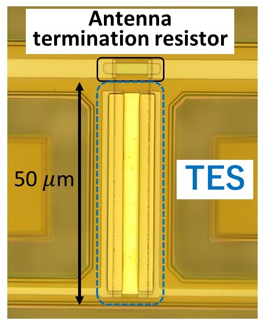
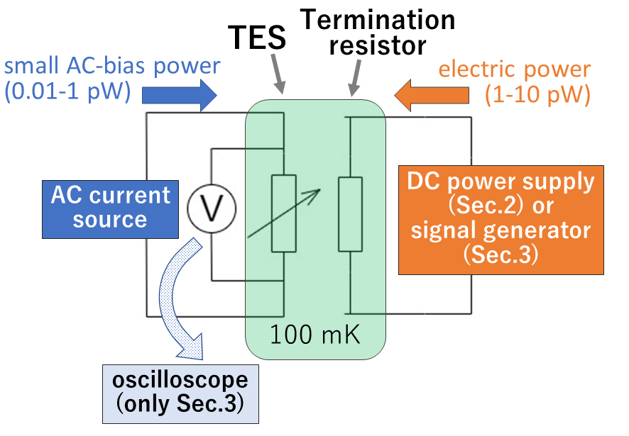
Figure 1: Left: the photograph of the measured bolometer sample. The antenna termination resistor is thermally coupled with the TES. Right: the circuit of the measurement setup. TES was biased with small AC power. An oscilloscope was used only in the time constant measurement (Sec. 3). A DC power supply (Sec. 2) or a signal generator (Sec. 3) provided electric power to the termination resistor. (Color figure online)

2.2 Evaluation method and results

We defined $P_{\mathrm{sat}}$ as equivalent to $P_{\mathrm{bath}}(T_{\mathrm{c}})$, which is the power flow to the heat bath when the TES island temperature is at critical temperature $T_{\mathrm{c}}$. This can be expressed using the bath temperature $T_{\mathrm{b}}$, index $n$, and $G$ Irwin2005 :

$$P_{\mathrm{sat}}=P_{\mathrm{bath}}(T_{\mathrm{c}})=K(T_{\mathrm{c}}^{n}-T_{\mathrm{b}}^{n})={\color[rgb]{0,0,0}\frac{G}{nT_{\mathrm{c}}^{n-1}}}(T_{\mathrm{c}}^{n}-T_{\mathrm{b}}^{n})$$ (1)

where the thermal conductivity at $T_{\mathrm{c}}$ is well defined using constant $K$ as $G=\mathrm{d}P_{\mathrm{bath}}(T)/\mathrm{d}T|_{T_{\mathrm{c}}}=nKT_{\mathrm{c}}^{n-1}$. At steady state, $P_{\mathrm{bath}}=P_{\mathrm{opt}}+P_{\mathrm{bias}}$, where $P_{\mathrm{opt}}$ is the optical power TES receives, and $P_{\mathrm{bias}}$ is the TES bias power. In our measurements, $P_{\mathrm{opt}}$ was replaced with the DC electric power dissipated in the resistor, $P_{\mathrm{res}}$ ($\sim$1-10 pW), and $P_{\mathrm{bias}}$ ($\sim$ 0.01 pW) could be neglected. Therefore, we assumed that $P_{\mathrm{bath}}=P_{\mathrm{res}}$.

First, we measured the TES resistance $R$ while sweeping $T_{\mathrm{b}}$ without applying $P_{\mathrm{res}}$ and then determined $T_{\mathrm{c}}$ from the $R$-$T_{\mathrm{b}}$ curve. The small bias power in our method enables the measurement of $T_{\mathrm{c}}$ at zero current; increasing the current may shift and widen the transition Bennett2012 . Next, we applied DC power to the termination resistor and repeated the $R$-$T_{\mathrm{b}}$ curve measurement. Figure 2 (left) shows the result of the $R$-$T_{\mathrm{b}}$ curves of one bolometer for various $P_{\mathrm{res}}$. To consider systematic errors, the error bars were re-scaled so that the reduced chi square reached 1. We found that the transition occurred at lower $T_{\mathrm{b}}$ when higher $P_{\mathrm{res}}$ was applied. From the $R$-$T_{\mathrm{b}}$ curves, we determined $T_{\mathrm{b,trans}}$, which is $T_{\mathrm{b}}$ in transition with a given $P_{\mathrm{res}}$. Figure 2 (right) shows the relation between $P_{\mathrm{res}}$ and $T_{\mathrm{b,trans}}$ of five TES samples with different leg length. The data were fitted with Eq. eq:Psat to estimate $G$ and $n$. Then we determined $P_{\mathrm{sat}}$ at the nominal operating temperature of 100 mK.

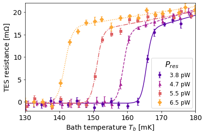
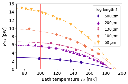
Figure 2: Left: the measured resistance of one sample (100 $\mu$m leg length) as a function of bath temperature for various $P_{\mathrm{res}}$. The error bars were calculated by the standard deviation from multiple measurements and the systematics. Right: the relation between $P_{\mathrm{res}}$ and $T_{\mathrm{b,trans}}$ of five samples with different leg length $\ell$. The lines show fitting results with Eq. eq:Psat. $P_{\mathrm{sat}}$ at 100 mK was estimated from the fitting lines as the red vertical line shows. (Color figure online)

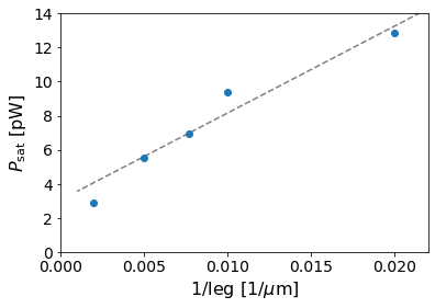
Figure 3: The measured $P_{\mathrm{sat}}$ as a function of the inverse leg length. The dashed line is a linear fit. (Color figure online)

The results of $G,n,$ and $P_{\mathrm{sat}}$ are shown in Table 1. All estimated $n$ values of the five samples were around 3, which is reasonable because $n$ is the thermal conductance index and was expected to be between 2 and 4 due to the material’s properties Mather1982 . $P_{\mathrm{sat}}$ was expected to be inversely proportional to the leg length suzuki2013multichroic ; koopman2018 . As shown in Figure 3, we confirmed the overall trend between $P_{\mathrm{sat}}$ and the inverse leg length, although the linear fit result was influenced by possible systematic effects, such as the extra systematic errors in $P_{\mathrm{sat}}$ fitting and slight geometrical variation of the five samples.

Table 1: The estimated parameters of five TES samples with different leg length $\ell$. The error of $T_{\mathrm{c}}$ comes from fitting of $R$-$T_{\mathrm{b}}$ curve. The errors of $G$ and $n$ come from fitting of $P_{\mathrm{res}}$-$T_{\mathrm{b,trans}}$ curve. $P_{\mathrm{sat}}$ at 100 mK was determined using $G$ and $n$.

ID	$\ell$ [$\mu$m]	$T_{\mathrm{c}}$ [mK]	$G$ [pW/K]	$n$	$P_{\mathrm{sat}}$(100 mK) [pW]
1	500	187.7 $\pm$ 0.2	53 $\pm$ 4	2.9 $\pm$ 0.4	2.86 $\pm$ 0.06
2	200	186.6 $\pm$ 0.2	103 $\pm$ 1	2.93 $\pm$ 0.03	5.51 $\pm$ 0.04
3	130	185.7 $\pm$ 0.2	129 $\pm$ 4	2.9 $\pm$ 0.2	6.9 $\pm$ 0.1
4	100	192.1 $\pm$ 0.1	172 $\pm$ 1	3.03 $\pm$ 0.03	9.38 $\pm$ 0.03
5	50	190.0 $\pm$ 0.3	248 $\pm$ 1	3.20 $\pm$ 0.03	12.86 $\pm$ 0.03

3 Time Constant Measurement

3.1 Setup

To measure the intrinsic time constant $\tau_{0}$, we applied AC electric power to the termination resistor, and measured the phase shift of the TES output voltage that was modulated by the electric power. The measurement setup was almost the same as that of the $P_{\mathrm{sat}}$ measurement as described in Section 2, except for two differences. Instead of a DC power supply, we used a signal generator to provide differential signals consisting of DC power plus a small amount of sinuous power. The AC resistance bridge can output a raw analog signal of TES voltage as well as a digital signal, so we measured the analog output signal using an oscilloscope.

3.2 Evaluation method and results

The TES thermal differential equation is shown below Irwin2005 :

$$C\frac{\mathrm{d}T}{\mathrm{d}t}=-P_{\mathrm{bath}}+P_{\mathrm{bias}}+P_{\mathrm{opt}}$$ (2)

where $T$ is the TES temperature. We considered a case where the TES is in transition with a small signal limit and $P_{\mathrm{bath}}=P_{\mathrm{bath}0}+G\Delta T$, where $P_{\mathrm{bath}0}$ is $P_{\mathrm{bath}}$ at steady-state. In our measurement $P_{\mathrm{bias}}$ ($\sim$0.1 pW) is negligible. $P_{\mathrm{opt}}$ is replaced with a DC offset plus small sinuous electric power with $f_{\mathrm{res}}$ applied to the termination resistor, $(P_{\mathrm{opt}}=)$ $\,P_{0}+\Delta P(t)=P_{0}+P_{\mathrm{res}}\cos(2\pi f_{\mathrm{res}}t)$. We can rewrite Eq. eq:thermal and solve the differential equation for $\Delta T(t)$:

$$\Delta T(t)=\frac{P_{\mathrm{res}}}{G}\left[\frac{1}{\sqrt{1+(2\pi f_{\mathrm{res}}\tau_{0})^{2}}}\cos\left(2\pi f_{\mathrm{res}}t+\phi(f_{\mathrm{res}})\right)\right]$$ (3)

where

$$\phi(f_{\mathrm{res}})=-\arctan(2\pi f_{\mathrm{res}}\tau_{0})$$ (4)

is the phase shift due to the electric power and $\tau_{0}=C/G$. We can write the TES resistance $R(t)$ as $R_{\mathrm{bias}}(1+\alpha\Delta T/T_{\mathrm{c}})$, neglecting the TES current term. When we bias TES with the AC current $I(t)=I_{\mathrm{bias}}\cos(2\pi f_{\mathrm{TES}}\,t)$, the TES output voltage $V=R(t)I(t)$ is:

$$V=R_{\mathrm{bias}}I_{\mathrm{bias}}\left[\cos(2\pi f_{\mathrm{TES}}\,t)+A\left(\cos(2\pi(f_{\mathrm{res}}+f_{\mathrm{TES}})t+\phi)+\cos(2\pi(f_{\mathrm{res}}-f_{\mathrm{TES}})t+\phi)\right)\right]$$ (5)

where $A=\alpha P_{\mathrm{res}}/(2GT_{\mathrm{c}}\sqrt{1+(2\pi f_{\mathrm{res}}\tau_{0})^{2}})$. We measured $\phi$ from the TES output voltage (Eq. eq:TESvolt) and estimated $\tau_{0}$ from Eq. eq:phase2tau0.

We set $P_{0}=$ 6.3 pW, which almost corresponds to the measured $P_{\mathrm{sat}}$, and $P_{\mathrm{res}}=$ 0.15 pW, which is $\sim$2% of $P_{\mathrm{sat}}$. We swept $f_{\mathrm{res}}$ from 10 to 50 Hz for 4 hours, over which the bath temperature of $\sim$100 mK and the TES resistance on transition were kept stable. We measured the TES voltage with an oscilloscope over 64 seconds for each $f_{\mathrm{res}}$ with a sampling rate of 3 kHz. Figure 5 shows an example of the time-ordered output signals with $f_{\mathrm{res}}$ of 16 Hz and $f_{\mathrm{TES}}$ of 9.8 Hz.

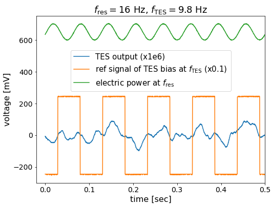
Figure 4: The example of the time-ordered signals ($f_{\mathrm{res}}=16$ Hz, $f_{\mathrm{TES}}=9.8$ Hz). The blue line is the TES output signal amplified by $10^{6}$, orange is the reference square signal of $P_{\mathrm{bias}}$ at $f_{\mathrm{TES}}$, and green is the electric power including the DC offset and small sinuous wave at $f_{\mathrm{res}}$. (Color figure online)

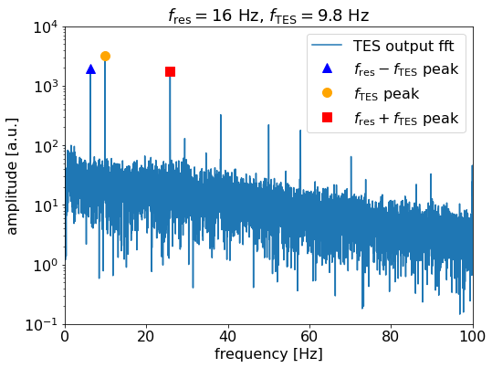
Figure 5: The amplitude of the Fourier transform of TES output signal ($f_{\mathrm{res}}=16$ Hz, $f_{\mathrm{TES}}=9.8$ Hz). The square and triangle mark correspond to the components of frequency $(f_{\mathrm{res}}\pm f_{\mathrm{TES}})$. (Color figure online)

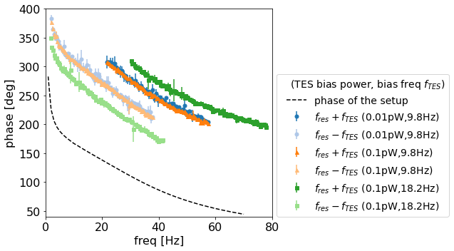
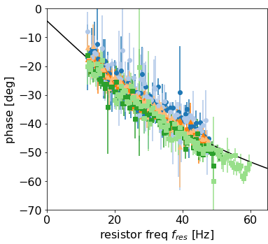
Figure 6: Left: the phase of $f_{\mathrm{res}}\pm f_{\mathrm{TES}}$ components measured at various $P_{\mathrm{bias}}$ (0.01 or 0.1 pW) and $f_{\mathrm{TES}}$ (9.8 or 18.2 Hz). Note that the x-axis is the actual frequency, not $f_{\mathrm{res}}$. The dashed line is the phase of the measurement setup. Right: the phase after subtraction of the phase of the measurement setup as a function of $f_{\mathrm{res}}$. The solid line is a fit result. (Color figure online)

The analysis procedure consisted of four steps: (I) A template signal was made by mixing the resistor signal (Fig. 5 green) with the TES input square signal, which had an amplitude of 5V TTL (Fig. 5 orange) in the time domain. The TES input square signal was provided by the AC resistance bridge and synchronized to $f_{\mathrm{TES}}$, so the template signal had two components proportional to $\cos(2\pi(f_{\mathrm{res}}\pm f_{\mathrm{TES}})t)$. (II) To extract the information of the modulated waves from the TES output signal, $\cos(2\pi(f_{\mathrm{res}}\pm f_{\mathrm{TES}})t)$, the Fourier transform of the TES output signal (Fig. 5) was cross-correlated with the Fourier transform of the template from step (I). (III) The phase of the modulated waves was computed, and (IV) the phase delay due to the measurement setup, including the preamplifier and wirings, was subtracted as shown in Figure 6.

The phases are consistent after subtraction of that of the measurement setup in all measurement conditions (Fig. 6 right), even though we measured the phase shift with different $f_{\mathrm{res}}$ and TES bias power. The data were fitted with Eq. eq:phase2tau0 plus a DC offset $\phi_{0}$: $\phi=-\arctan(2\pi f_{\mathrm{res}}\tau_{0})+\phi_{0}$. $\tau_{0}$ of the TES sample was estimated as 3.0 $\pm$ 0.1 msec, while $\phi_{0}$ was estimated as -4.6 $\pm$ 0.8 deg. The systematic error of $\tau_{0}$ was estimated to be 0.6 msec, which is the difference of the fits between free $\phi_{0}$ and fixed $\phi_{0}=0$. The measured value of $\tau_{0}$ is consistent with the expected value within a factor of 2, considering the estimated value of $C$ (0.28 pJ/K) from the specific heat of the normal metal on the bolometer island rayne1957 and the measured value of $G$ (129 pW/K) with the method described in Section 2.

4 Conclusion

We demonstrated evaluation methods for TES parameters by applying DC or AC electric power to simulate optical power. These methods enabled us to evaluate $P_{\mathrm{sat}}$ and $\tau_{0}$ without electrothermal feedback because only small TES bias power is applied. These methods are necessary to characterize TES samples and to provide feedback for the fabrication and development of TES bolometers for future CMB experiments abazajian2016 .

- (1) K. Irwin, G. Hilton, in Topics Appl. Phys., vol. 99 (2005), pp. 63–150
- (2) S. Adachi, et al., The Astrophysical Journal 897(1), 55 (2020)
- (3) S.K. Choi, et al., Journal of Cosmology and Astroparticle Physics 2020(12), 045 (2020)
- (4) J. Sayre, et al., Physical Review D 101(12), 122003 (2020)
- (5) P. Ade, et al., Physical review letters 127(15), 151301 (2021)
- (6) C.A. Hill, et al., in Millimeter, Submillimeter, and Far-Infrared Detectors and Instrumentation for Astronomy IX, vol. 10708 (SPIE, 2018), vol. 10708, pp. 698–718
- (7) J.C. Mather, Applied Optics 21(6), 1125 (1982)
- (8) N.F. Cothard, et al., in Millimeter, Submillimeter, and Far-Infrared Detectors and Instrumentation for Astronomy X, vol. 11453 (2020), vol. 11453, p. 1145325
- (9) B. Westbrook, et al., Journal of Low Temperature Physics 193(5), 758 (2018)
- (10) J.R. Stevens, et al., Journal of Low Temperature Physics pp. 1–9 (2020)
- (11) D.A. Bennett, et al., J Low Temp Phys 167, 102 (2012). DOI 10.1007/s10909-011-0431-4
- (12) A. Suzuki, Multichroic bolometric detector architecture for cosmic microwave background polarimetry experiments. Ph.D. thesis, UC Berkeley (2013)
- (13) B.J. Koopman, et al., Journal of Low Temperature Physics 193(5), 1103 (2018)
- (14) J.A. Rayne, Physical Review 107(3), 669 (1957)
- (15) K.N. Abazajian, et al., arXiv preprint arXiv:1610.02743 (2016)