The GW-Universe Toolbox III: simulating joint observations of gravitational waves and gamma-ray bursts

Abstract

Context. In the current multi-messenger astronomy era, it is important that information about joint gravitational wave (GW) and electromagnetic (EM) observations through short gamma-ray burst (sGRBs) remains easily accessible to each member of the GW-EM community. The possibility for non-experts to execute quick computations of joint GW-sGRB detections should be facilitated.

Aims. In this study, we construct a model for sGRBs and add this to the framework of the previously-built Gravitational Wave Universe Toolbox (GWToolbox or Toolbox). We provide expected joint GW-sGRB detection rates for different combinations of GW detectors and high-energy (HE) instruments.

Methods. We employ and adapt a generic GRB model to create a computationally low-cost top-hat jet model suitable for the GWToolbox. With the Toolbox, we simulate a population of binary neutron stars (BNSs) observed by a user-specified GW detector such as LIGO, Virgo, the Einstein Telescope (ET) or the Cosmic Explorer (CE). Based on the characteristics of each binary, our model predicts the properties of a resulting sGRB, as well as its detectability for HE detectors such as Fermi/GBM, Swift/BAT or GECAM.

Results. We report predicted joint detection rates for combinations of GW detectors (LIGO and ET) with HE instruments (Fermi/GBM, Swift/BAT, and GECAM). Our findings stress the significance of the impact that ET will have on the multi-messenger astronomy; where the LIGO sensitivity is currently the limiting factor regarding the number of joint detections, ET will observe BNSs at such a rate, that the vast majority of detected sGRBs will have a GW counterpart observed by ET. These conclusions hold for CE as well. Additionally, since LIGO can only detect BNSs up to redshift $\sim$0.1 where few sGRBs exist, a search for sub-threshold GW signals at higher redshifts using sGRB information from HE detectors has the potential to be very successful and significantly increase the number of joint detections. Equivalently, during the ET era, GW data can assist in finding sub-threshold sGRBs, potentially increasing e.g. the number of joint ET-Fermi/GBM observations by $\sim$270%. Lastly, we find that our top-hat jet model underestimates the number of joint detections that include an off-axis sGRB. We correct for this by introducing a second, wider and weaker jet component. We predict that the majority of joint detections during the LIGO/Virgo era will include an off-axis sGRB, making GRB170817A not as unlikely as one would think based on the simplest top-hat jet model. In the ET era, most joint detections will contain an on-axis sGRB.

1 Introduction

Nearly five years after the first joint observation of a gravitational wave (GW) signal and a short gamma-ray burst (sGRB) from a binary neutron star (BNS) merger (Abbott et al., 2017b, a; Goldstein et al., 2017), multi-messenger astronomy has established itself as a central part of modern astrophysics. The ability to observe astrophysical events both gravitationally and electromagnetically allows for unique insights into (astro)physical phenomena, potentially probing new fundamental understandings in physics. The implications of multi-messenger astrophysics stretch beyond GW physics, as this concept can be applied to many different areas within physics and astrophysics. For example, one can use joint detections to compute the Hubble constant (e.g. Chen et al. (2021b, a)), rule out or confirm certain binary progenitor models (e.g. Eichler et al. (1989)), improve our understanding on neutron star (NS) interior and equation-of-state (EOS) (e.g. Metzger (2019)), or carry out tests of general relativity (e.g. Kim, 2021; Clark et al., 2015). The number of joint observations will only increase in the near future; BNS and black hole - neutron star (BHNS) mergers, the main candidates for joint detections due to their production of GW signals as well as electromagnetically sGRBs, will be observed more frequently. Current detectors such as aLIGO (Harry & the LIGO Scientific Collaboration, 2010) and Virgo (Acernese et al., 2015) will eventually operate at their design sensitivities, and the planned Einstein Telescope (ET, Punturo et al. (2010)) and Cosmic Explorer (CE, Reitze et al. (2019)) will observe GW sources at an unprecedented rate in this frequency band ($\sim$10 - 1000 Hz). Additionally, next to already established high-energy (HE) detectors such as Fermi/GBM (Meegan et al., 2009) and Swift/BAT (Gehrels et al., 2004), newer instruments like Insight-HXMT (Song et al., 2022) and GECAM-GRD (Xiao et al., 2022; Zhang et al., 2019) (launched in 2017 and 2020 respectively) will prove extremely useful in the search of sGRBs as electromagnetic (EM) counterparts to GW observations.

Previously, we built a open-source Python based software, the Gravitational Wave Universe Toolbox (Yi et al., 2021, 2022, the GWToolbox or Toolbox hereafter for short) to make GW astrophysics easily accessible. The GWToolbox can be found at gw-universe.org, or downloaded as a Python package at https://bitbucket.org/radboudradiolab/gwtoolbox. The GWToolbox can be used to simulate observations with different kinds of GW detectors on various common GW source populations, among which are BNS and BHNS mergers. It can return a synthetic catalogue of BNS/BHNS, which could be detected with a user-specified GW detector, signal-to-noise (SNR) threshold and observation duration. For each event in the catalogue, the Toolbox returns the masses of the binary, luminosity distance, orbital inclination and effective spin. We have now added to this a sGRB model that allows the Toolbox to return the properties of a potential sGRB from these sources as observed by a user-selected HE detector. This enables the user to study the detectability of these events as GRB with respect to a certain HE detector, and investigate joint GW-EM detection rates. This new functionality makes the GWToolbox a multi-messenger simulator, and paves the way towards more applications in studies such as prospects of joint-detections with different GW/HE detectors and sub-threshold strategies, GRB physics and compact binary merger history. The first study is conducted in this work, while we will discuss in more detail several planned other projects in Section 4. Where this research is in a sense similar to a recent study by Ronchini et al. (2022), it should be noted that our project touches upon several slightly different aspects of the prospects of multi-messenger astronomy, meaning that these two studies can be viewed as complementary to one another.

In this paper, we describe the sGRB model that has been added to the Toolbox, as well as investigate joint detection rates predicted by the upgraded GWToolbox. The paper is organised as follows: in Section 2, we will first give a brief introduction on how the GWToolbox gives the synthetic catalogue of BNS/BHNS. Then we describe how GRBs emission from a BNS/BHNS progenitor is simulated in our model, and how we determine the detectability of the GRB for a certain HE detector. In Section 3, we first reproduce individual and population properties of historical GRBs, and by doing that we fix the parameters in the underlying population and GRB models. Subsequently, we use the simulation to predict future detection rates, with different combinations of GW/HE detectors, with sub-threshold joint-observation strategies, and specifically for off-axis sGRBs. In Section 4 we summarise our findings and provide future prospects.

2 Methods

2.1 The GWToolbox: producing a synthetic GW catalogue

Here we give a brief explanation on how a synthetic GW catalogue is generated in the GWToolbox. For a detailed description, we refer to Yi et al. (2021). For a certain GW detector, its noise power spectrum and the antenna pattern are denoted as $S_{n}(f)$ and $F_{+,\times}$ respectively. The $S_{n}(f)$ is either from literature if the GW detector is from a default list, or calculated with FINESSE (Brown et al., 2020) if it has a user-customised configuration. The detector response to the GW from a compact binary merger is:

$$h(f)=F_{+}h_{+}(f)+F_{\times}h_{\times}(f),$$ (1)

where $h_{+,\times}$ are the ”plus” and ”cross” polarisations of the GW waveform, which are calculated with a certain waveform approximant (e.g., IMRPhenomD, Husa et al. (2016); Khan et al. (2016)). The signal-to-noise ratio (S/N, SNR, or $\rho$) of the GW is calculated as:

$$\rho^{2}=4\int^{f_{\rm{high}}}_{f_{\rm{low}}}\frac{|h^{2}(f)|}{S_{\rm{n}}(f)}df.$$ (2)

For a certain S/N threshold, we can define a probability of detection of a source as:

$$\mathcal{D}(\mathbf{\Theta})=\oiint d\Omega d\Omega^{\prime}\mathcal{H}(\rho^{2}-\rho^{2}_{\star})/(4\pi)^{2},$$ (3)

$\mathbf{\Theta}$ denotes the intrinsic parameters (e.g., masses and effective spin, depending on the waveform approximant) and the luminosity distance of the source, $\Omega$ and $\Omega^{\prime}$ denote the sky location angles ($\theta$, $\phi$), the inclination angle ($\iota$) and the polarisation angles ($\psi$); $\mathcal{H}$ is the Heaviside step function. With a merger rate model of the population, $\dot{n}(\mathbf{\Theta})$, the expected distribution of detectable sources is:

$$N_{\rm{D}}(\mathbf{\Theta})=\frac{T}{1+z}\frac{dV_{\rm{c}}}{dz}\dot{n}(\mathbf{\Theta})\mathcal{D}(\mathbf{\Theta}),$$ (4)

and the expected number of detection is an integration of $N_{\rm{D}}(\mathbf{\Theta})$ over the possible parameter space. A synthetic catalogue is obtain by a MCMC sampling from $N_{\rm{D}}(\mathbf{\Theta})$. Fig. 1 is an example of the simulated catalogues from the GWToolbox. The GWToolbox has one default parameterised BNS model (pop-A) and two BHNS population models (pop-A and pop-B). For a detailed description of these population models, we refer to Yi et al. (2021). The common hyper-parameters for BNS, BHNS-pop-A and pop-B are listed in Tab. 1 (including hyper-parameters for the GRB model, which will be introduced in Sec. 2.3). For BNS, there are five extra hyper-parameters describing the mass distribution of the NS, and its effective spin. In our treatment, we assume no dependence of the GRB properties on these parameters. For BHNS-pop-A, there are 9 extra parameters describing the masses distribution of BH and NS, and their effective spin. The values of these hyper-parameters influence the fraction of BHNS system which passes the $R_{\rm{tid}}>R_{\rm{ISCO}}$ criterion (see Sec. 2.2). We list these hyper-parameters and their default values in Tab. 2. The difference between BHNS-pop-A and pop-B is that the latter includes another Gaussian mass peak centered at $\sim 40\,M_{\odot}$ on the mass function of pop-A to take into account the BH originated from pair-instability supernovae.

Hyper-parameter	Description	Default value
$R_{\rm{n}}$	Normalisation factor of the cosmic merger rate of BNS merger	50 Gpc-3 yr-1
$\tau$	the averaged time-delay between the binary star formation and BNS merger	10 Gyr
$\Delta\theta_{\rm{mean}}$	Mean jet opening angle	15∘
$\Delta\theta_{\rm{std}}$	Standard deviation of the jet opening angle	4∘
$\log r_{0,\rm{mean}}$	Mean log GRB radius	13 $\log\text{cm}$
$\log r_{0,\rm{std}}$	Standard deviation of log GRB radius	0.1 $\log\text{cm}$
$\log E_{\rm{GRB,mean}}$	Mean of total GRB energy	49.3 $\log\text{ergs}$
$\log E_{\rm{GRB,std}}$	Standard deviation of total GRB energy	0.5 $\log\text{ergs}$
$\nu^{\prime}_{0,\rm{mean}}$	the mean value of the reference frequency in the jet co-moving frame	0.001 MeV
$\nu^{\prime}_{0,\rm{std}}$	Standard deviation of the reference frequency in the jet co-moving frame	0.00075 MeV
$\gamma_{\rm{mean}}$	Mean of the bulk Lorentz factor	250
$\gamma_{\rm{std}}$	Standard deviation of the bulk Lorentz factor	75
$t_{d,std}$	Standard deviation of the time delay $t_{d}$	0.4 s

Table 1: Common hyper-parameters for both BNS/BHNS originated GRB population model. Their default values are listed in the third column, with which, the historical observation can be optimally reconstructed.

Hyper-parameter	Description	Default value
$m_{\rm{n,mean}}$	The mean of NS masses	1.4 $M_{\odot}$
$m_{\rm{n,std}}$	The standard deviation of NS masses	0.5 $M_{\odot}$
$m_{\rm{n,high}}$	The higher limit of NS masses	2.5 $M_{\odot}$
$\gamma$	the power index of the mass function tail	2.5
$c$	$c/\gamma+\mu$ is the peak mass of BH mass function	15
$m_{\bullet,\rm{cut}}$	the upper limit of BH mass	95 $M_{\odot}$
$\chi_{\rm{eff}}$	the standard deviation of the effective spin parameters	0.1

Table 2: Extra hyper-parameters of the underlying BHNS population of model pop-A.

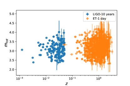
Figure 1: Redshift distribution of a simulated BNS merger catalogue from the GWToolbox for a LIGO observation time of 10 years (blue) and 1 day of ET observations (orange).

The catalogue simulated in this way does not include the orbital inclination angles, since the angles are marginalised when calculating the probability of detection. Since the inclination angle $\iota$ is a crucial property of GRBs, we want to recover $\iota$ from $\mathcal{D}(\mathbf{\Theta})$. We note that $\mathcal{D}(\mathbf{\Theta})$ is equivalent to the fraction in a uniform sample of $(\theta,\phi,\iota,\psi)$ that results in $\rho\geq\rho_{\star}$. We know:

$$\rho\propto\sqrt{\left(\frac{1+\cos^{2}\iota}{2}\right)^{2}F_{+}^{2}+\cos\iota^{2}F_{\times}^{2}},$$ (5)

where we define the right-hand side as $\bar{\rho}$. For a GW event in the catalogue, with a detection probability $\mathcal{D}$: we draw a sample of uniformly distributed $(\theta,\phi,\iota,\psi)$, and calculate the corresponding $\bar{\rho}$. We randomly select a $\tilde{\rho}$ which is larger than the $(1-p)$-th quantile. The corresponding $\iota$ is assigned as the inclination angle of the source. In Fig. 2, we plot the distribution of $\iota$ of the simulated detected sample of BNSs. We can find in the histogram that for $\rho_{\star}=0$, $\iota$ follows an isotropic distribution ($\sin\iota$). When $\rho_{\star}=8$, the distribution of $\iota$ peaks at around $\sim 30^{\circ}$. This is a result of the increasing GW signal towards lower inclinations combined with the $\sin\iota$ of the solid angle.

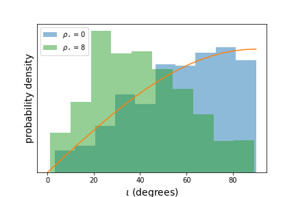
Figure 2: Inclination angle distribution of GW detection of different S/N threshold.

2.2 BNS and BHNS mergers that result in a sGRB

In general, the merger remnant after a BNS or BHNS is only able to produce a sGRB if it is surrounded by a sizeable accretion disk powering a relativistic jet (e.g. Bernuzzi, 2020; Fryer et al., 2015; Zhang, 2018). For BNS systems, in cases when the binary promptly collapses to a black hole (BH), it is known that the remnant satisfies this criterion. However, depending on the initial binary mass, different scenarios are possible for the final fate of the BNS merger remnant: apart from a BH, a BNS may form a short-lived hyper- or supermassive NS collapsing to a BH, or result in an infinitely stable supermassive NS (e.g. Ciolfi, 2018). There still exists uncertainty regarding the ability of a NS remnant to contain an accretion disk and relativistic jet. However, recent observations as well as numerical evidence suggest that NS remnants may indeed launch jets resulting in a sGRB (Sarin & Lasky, 2020). As such, in the Toolbox, we assume that all of the simulated BNSs will launch a relativistic jet after merger, triggering a sGRB.

For a BHNS system, only in the case that the NS is swallowed by the BH before it is tidally disrupted, there will be no associated EM counterpart (Fryer et al., 2015). Therefore, we impose a condition for the association of a prompt GRB with a BHNS as:

$$R_{\rm{tid}}>R_{\rm{ISCO}},$$ (6)

where $R_{\rm{tid}}$ is the tidal radius, within which the NS will be tidally disrupted by the BH. It can be calculated with:

$$R_{\text{tid}}=\big{(}\frac{M_{\bullet}}{M_{\rm{NS}}}\big{)}^{1/3}R_{\rm{NS}},$$ (7)

where $M_{\bullet}$ and $M_{\rm{NS}}$ are masses of the BH and NS respectively, and $R_{\rm{NS}}$ is the radius of the NS. $R_{\rm{ISCO}}$ is the radius of the Innermost Stable Circular Orbit (ISCO) around the BH, within which the NS is thought to be swallowed by the BH. The component masses of the BHNS are outputs from the GW catalogue of the Toolbox. However, the $R_{\rm{NS}}$ depends on the mass-radius-relation of a NS. Therefore, in the GWToolbox, we build in four possible mass-radius-relations (MRRs): one relativistic Brueckner-Hartree-Fock EoS (MPA1) (Müther et al., 1987), two relativistic mean-field theory EOSs (MS0, MS2) (Müller & Serot, 1996), and one nonrelativistic potential model (PAL1) (Prakash et al., 1988). In general, any tabulated MRR can be incorporated.

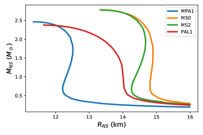
Figure 3: Built-in MRRs in the GWToolbox. We use the Brueckner-Hartree-Fock EoS (MPA1), two relativistic mean-field theory EOSs (MS0, MS2), and one nonrelativistic potential model (PAL1).

2.3 The sGRB model

With a catalogue of GRB progenitors, we still need a GRB emission model so as to simulate the GRB from those progenitors. Here we employ and adapt a generalised geometrical model for GRBs from Ioka & Nakamura (2001), which is independent of the details of the physics, and is therefore compatible with various physical GRB models. Its mathematical structure allows for potential future adaptations for an increased complexity and accuracy to be easy to implement. Additionally, it serves the purpose of the Toolbox: while it should recover the GRB with a reasonable accuracy, its simplicity keeps the computational cost low allowing for quick computations. The core quantity is the observed flux at the observed instance $T$:

$$F_{\nu}(T)=\frac{\nu D}{\gamma\beta}\int^{2\pi}_{0}\phi\int^{\alpha_{m}}_{0}\alpha^{2}d\alpha\int^{\nu\gamma(1+\beta)}_{\nu\gamma(1-\beta)}\frac{d\nu^{\prime}}{\nu^{\prime}}\frac{j^{\prime}_{\nu^{\prime}}}{(1-\mu^{2})^{3/2}},$$ (8)

where $\gamma$ is the bulk Lorentz factor of the jet, $\beta=\sqrt{1-\gamma^{2}}$; $\alpha$, $\alpha_{m}$ and $\mu$ are geometry parameters describing the relative position between the emitting region and the observer. $j^{\prime}_{\nu^{\prime}}$ is the emissivity in the jet-comoving frame, which is assumed to be isotropic. For more details, see Ioka & Nakamura (2001) as well as Woods & Loeb (1999) & Piran (1999).

The emissivity $j^{\prime}_{\nu\prime}$ is constructed as follows:

$$j^{\prime}_{\nu^{\prime}}=A_{0}f(\nu^{\prime})\pi(t)\psi(r)\Pi(\Omega),$$ (9)

where $\pi(t)$ and $\psi(r)$ are, respectively, the temporal and radial distribution of the emission, in the comoving frame. $\Pi(\Omega)$ is the angular structure of the jet, $A_{0}$ is a constant, and $f(\nu^{\prime})$ denotes the spectrum in the comoving frame. Here, we employ the most simplified case, where a top-hat jet with instantaneous emission at time $t_{0}$ and radius $r_{0}$ is assumed. We get:

$$\pi(t)=\delta(t-t_{0}),$$ (10)

$$\psi(r)=\delta(r-r_{0}),$$ (11)

$$\begin{split}&\Pi(\Omega)=H(\Delta\theta-|\theta-\theta_{v}|)\\ &\qquad H\left[\cos\phi-\left(\frac{\cos\Delta\theta-\cos\theta_{v}\cos\theta}{\sin\theta_{v}\sin\theta}\right)\right].\end{split}$$ (12)

$\Delta\theta$ and $\theta_{v}$ are the half-opening angle and viewing angle of the jet, respectively. For the spectrum $f(\nu^{\prime})$, we use the shape of the Band function (Band et al., 1993):

$$f(\nu^{\prime})=\big{(}\frac{\nu^{\prime}}{\nu^{\prime}_{0}}\big{)}^{1+\alpha_{B}}\big{(}1+\frac{\nu^{\prime}}{\nu^{\prime}_{0}}\big{)}^{(\alpha_{B}-\beta_{B})/s}.$$ (13)

We set $\alpha_{B}=-1$, $\beta_{B}=-2.2$, and $s=1$, as these are typical values resulting in a spectrum whose shape matches the Band spectrum (Preece et al., 2000; Ioka & Nakamura, 2018). With the assumptions of Eqs. 10-12, Eq. 8 becomes

$$F_{\nu}(T)=\frac{2cA_{0}r_{0}\gamma^{2}}{D^{2}}\frac{\Delta\phi(T)f\big{(}\nu\gamma(1-\beta\cos\theta(T))\big{)}}{\bigg{(}\gamma^{2}\big{(}1-\beta\cos\theta(T)\big{)}\bigg{)}^{2}}.$$ (14)

We visualise the geometry of our setup in Fig. 4 for an off-axis (top) and on-axis GRB (bottom).

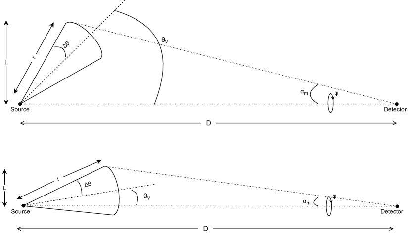
Figure 4: Schematic overview of the structure and geometry of our sGRB model, for a jet with opening angle $\Delta\theta$, viewing angle $\theta_{v}$ and distance to earth $D$. We depict an off-axis GRB in the top panel, while the bottom shows an on-axis one.

In equation (14), the constant $A_{0}$ is related to the total energy of the GRB ($E_{\rm{GRB}})$. In order to find the relation between $A_{0}$ and $E_{\rm{GRB}}$, we conduct the following derivation. In the comoving frame, the radiating energy of the ejecta is:

$$E^{\prime}_{\rm{GRB}}=\int j^{\prime}dV\int d\nu^{\prime}\int d\Omega\int dt,$$ (15)

where $j^{\prime}$ is the emissivity in the comoving frame, $\int dV$, $\int d\nu^{\prime}$, $\int d\Omega$ and $\int dt$ are integrals over volume, frequencies, emission directions and time respectively. Assuming isotropy of emission in the comoving frame, the direction integral gives $4\pi$, and with the assumption of instantaneous emission at an infinitely thin layer with a top-hat jet, the volume and time integrals give

$$\int dV\int dt=2\pi(1-\cos\Delta\theta)r^{2}_{0}.$$

The frequency integral of the Band spectrum gives

$$\int f(\nu^{\prime})d\nu^{\prime}=-A_{0}\nu^{\prime}_{0}\frac{s^{2}\Gamma(\frac{\alpha}{2}+1+\frac{2}{s})\Gamma(-\frac{\beta}{s}+1-\frac{2}{s})}{(\alpha+2)(\beta+2)|s|\Gamma(-\frac{\beta-\alpha}{2})}.$$

Therefore, equation (15) becomes:

$$E^{\prime}_{\rm{GRB}}=8\pi^{2}(1-\cos\Delta\theta)r^{2}_{0}A_{0}\mathcal{I}\nu^{\prime}_{0},$$ (16)

where

$$\mathcal{I}=-\frac{s^{2}\Gamma(\frac{\alpha}{2}+1+\frac{2}{s})\Gamma(-\frac{\beta}{s}+1-\frac{2}{s})}{(\alpha+2)(\beta+2)|s|\Gamma(-\frac{\beta-\alpha}{2})},$$

which is 6.64 when $s=1$, $\alpha=-1$ and $\beta=-2.2$. Note that energy is not Lorentz invariant, and in the observer frame, the energy transformed to:

$$E_{\rm{GRB}}=\gamma E^{\prime}_{\rm{GRB}}.$$ (17)

So, we have

$$E_{\rm{GRB}}=A_{0}\gamma 8\pi^{2}(1-\cos\Delta\theta)r^{2}_{0}A_{0}\mathcal{I}\nu^{\prime}_{0}.$$ (18)

Equivalently:

$$A_{0}=\frac{E_{\rm{GRB}}}{\gamma 8\pi^{2}(1-\cos\Delta\theta)r^{2}_{0}A_{0}\mathcal{I}\nu^{\prime}_{0}}.$$ (19)

It should be noted that $E_{\text{GRB}}$ depends on the mass of the accretion disk surrounding the merger remnant as well as the accretion efficiency, both of which depend on the binary parameters (Bernuzzi, 2020; Fryer et al., 2015). Where efforts have been made to connect these quantities (e.g. Radice et al. (2018); Bernuzzi et al. (2020); Nedora et al. (2020)), as of yet the exact relationship between the binary properties and GRB energy is not known. As such, taking $E_{\text{GRB}}$ as a direct free parameter instead of indirectly through e.g. the binary mass is currently the safest option. More so, the total GRB energy is typically well-approximated by assuming a standard reservoir clustered around some central energy value (Frail et al., 2001; Zhang, 2018).

Note that equation (14) assumes an instantaneous emission from one location $r=r_{0}$ and $t=r_{0}/c$. The corresponding lightcurve is a single pulse which rises sharply at $T=0$ for on-axis cases. In reality the lightcurve is a superposition of multiple pulses, resulting in a more gradual rise. We recover this feature by implementing a temporally extended jet launch: every GRB pulse is launched with a different delay time $t_{\rm{d}}$ (in the source frame) relative to the merger, and $t_{\rm{d}}$ follows an extended probability distribution. The lightcurve can be obtained by convolving the original lightcurve with the probability distribution of (the red-shifted) $t_{\rm{d}}$, for which we use a Gaussian with a width $t_{\rm{d},std}(1+z)$, centred at $3t_{\rm{d},std}(1+z)$.

As a summary, our GRB requires the following parameters.
Intrinsic parameters:

• $\gamma$: the bulk Lorentz factor of the jet;

• $r_{0}$: the radius from the central engine, where the gamma-ray emission happens;

• $E_{GRB}$: the total energy released into prompt gamma-ray, in the observer frame, this is related with the normalization parameter $A_{0}$;

• $\alpha_{B}$, $\beta_{B}$, $s$ and $\nu^{\prime}_{0}$: intrinsic spectrum parameters;

• $\Delta\theta$: the half opening angle of the jet cone;

• $t_{\rm{d,std}}$ the standard deviation of the intrinsic jet launch delay time distribution.

Extrinsic parameters:

• $\iota$: the viewing angle of the observer, or equivalently, the inclination angle of the binary orbital plane;

• $D$ or $z$: the luminosity distance from the source to the observer, or equivalently, the red-shift of the GRB.

For each GRB in the Toolbox, the $\Delta\theta$, $\log r_{0}$, $\log E_{\rm{grb}}$, $\nu^{\prime}_{0}$, $\gamma$ are assigned as Gaussian randoms. The corresponding means and standard deviations are $\Delta\theta_{\rm{mean}}$ and $\Delta\theta_{\rm{std}}$, $\log r_{0,\rm{mean}}$ and $\log r_{0,\rm{std}}$, $\log E_{\rm{grb},\rm{mean}}$ and $\log E_{\rm{grb},\rm{std}}$, $\nu^{\prime}_{0,\rm{mean}}$ and $\nu^{\prime}_{0,\rm{std}}$, $\gamma_{\rm{mean}}$ and $\gamma_{\rm{std}}$ respectively. We summarise these hyper-parameters for the underlying GRB population in Tab.1. The inclination angle $\iota$ and the distance $D$ are taken directly from the GW part of the GWToolbox.

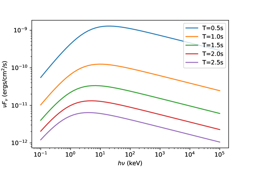
(a) The simulated time-evolving spectrum of the on-axis sGRB GRB131004A.

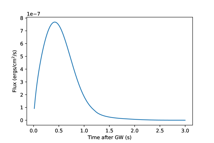
(b) The simulated lightcurve of the on-axis GRB131004A, within an energy range of 10-1000 keV.

Figure 5: Characteristics of a GRB131004A-like on-axis GRB, according to the GWToolbox. We use the following hyper-parameters: $\gamma=100$, $\log(r_{0}/\text{cm)}=12.93$, $\log(E_{\text{GRB}}/\text{ergs})=49.8$, $\nu_{0}^{\prime}=0.7$keV, $\Delta\theta=15^{\circ}$, $\theta_{v}=10^{\circ}$, and $z=0.717$.

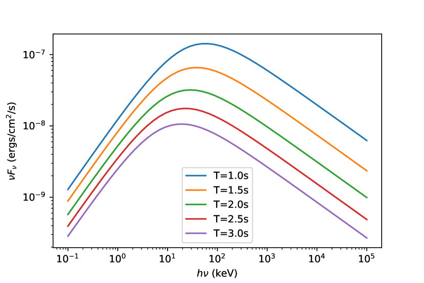
(a) The simulated time-evolving spectrum of the off-axis sGRB GRB170817A.

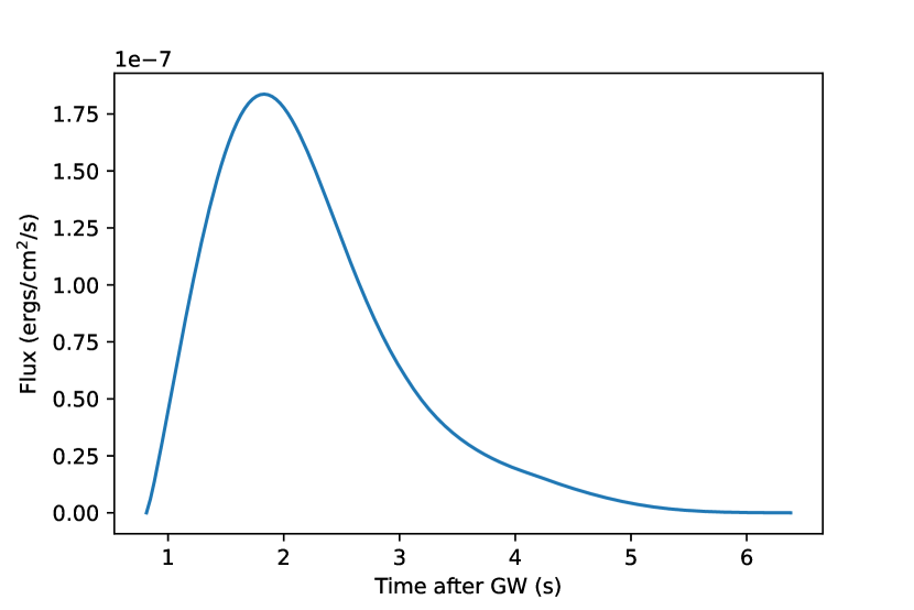
(b) The simulated lightcurve of the off-axis GRB170817A, within an energy range of 10-1000 keV.

Figure 6: Characteristics of a GRB170817A-like off-axis GRB, according to the GWToolbox. We use $\gamma=100$, $\log(r_{0}/\text{cm})=13.03$, $\log(E_{\text{GRB}}/\text{ergs})=49.65$, $\nu_{0}^{\prime}=8$ keV, $\Delta\theta=15^{\circ}$, $\theta_{v}=18.75^{\circ}$, and $z=0.0099$.

To illustrate and visualise the model, in Figs. 5 & 6 we show the time-evolving spectrum and lightcurve of an on- and off-axis sGRB respectively. The time-evolving spectrum $F_{\nu}(t)$ can be calculated with the method described above. The lightcurve, either in units of phs/s/cm² or ergs/s/cm², can be calculated with:

$$L_{\rm{ph}}(t)=\int\frac{F_{\nu}(t)}{h\nu}d\nu,$$ (20)

or

$$L_{\rm{ergs}}(t)=\int F_{\nu}(t)d\nu,$$ (21)

respectively, with the integral over the photon frequencies corresponding to the energy range of the detector. In Fig. 5, we attempt to recover the properties of the on-axis sGRB GRB131004A, observed by Fermi/GBM (von Kienlin et al., 2020; Gruber et al., 2014; von Kienlin et al., 2014; Bhat et al., 2016). With the hyper-parameters listed in Fig. 5, our model finds: $T_{90}=0.96$s (compared to an observed 1.152s), a fluence (10-1000 keV) of $5.64\times 10^{-7}$ (observed $5.099\times 10^{-7}$) ergs/cm², a 1-sec and 64-ms peak flux of respectively 5.85 (6.8) and 8.25 (9.8) ph/cm²/s, and $E_{\text{peak}}=118$ (observed 118 as well) keV. We also show the evolving spectrum and lightcurve according to our model in the same energy range, for the off-axis GRB170817A observed by Fermi/GBM (Goldstein et al., 2017) in Figs. 6(a) & 6(b). Here, we find $T_{90}=2.55$s (compared to an observed $2.0\pm 0.5$s), a fluence of $3.16\times 10^{-7}$ (observed $2.8\pm 0.2\times 10^{-7}$) ergs/cm², a 64-ms peak flux of 3.00 (compared to $3.7\pm 0.9$) ph/cm²/s, and an $E_{\text{peak}}$ of 130 keV (observed $185\pm 62$) keV. Overall, these predictions match the observations quite well for both GRBs. Still, for GRB170817A, we needed to choose quite an atypical value for $\nu_{0}^{\prime}$ in order to obtain somewhat realistic observables. This indicates that our top-hat jet model may contain several limitations which become exposed for off-axis GRBs, specifically regarding the angular dependence of the GRB spectrum; for a more detailed discussion, see Sec. 4 and Ioka & Nakamura (2019). Nonetheless, keeping in mind that we expect the majority of GRB observations to be on-axis, if its main limitation is an inaccurate computation of off-axis spectral peaks, our model is accurate enough to serve the purpose of the GWToolbox. The aim of the Toolbox is not to perfectly match all observations made by HE detectors; it should simply be able to recover the majority of the observations reasonably well, with low computational effort. This allows the user to make quick computations of joint detectabilities.

2.4 GRB detectability against HE detectors

Detector	Energy Range (keV)	Flux Limit	FoV (percentage)	$\mathbf{f_{c}}$
Compton-BATSE	50-300	0.3phs/cm2/s	25%	1
Swift/BAT	15-150	1.5 phs/cm2/s	10%	2
Fermi/GBM	10-1000	2.28 phs/cm2/s	60%	2
Insight-HE1	30-250	$2\times 10^{-8}$ ergs/s/cm2	60%	1
GECAM2	15-5000	$1.8\times 10^{-8}$ ergs/s/cm2	30%	1

• While we include Insight-HE in our list here, we leave this instrument out of our analysis; as its published GRB catalogue is currently incomplete, we are not able to extract an effective flux threshold at which it operates at the present time. Similarly to Fermi/GBM and Swift/BAT, using the theoretical threshold does not lead to accurate detection rates for sGRBs.

• The designed FoV of GECAM is 100%, however, due to a power problem, the actual on-orbit FoV had been only about $\sim 30\%$ for the past year. During the preparation of this manuscript, we learnt that the FoV has been restored to $\sim 60\%$ recently from a private conversation.

Table 3: Default parameters for built-in HE detectors. Please note: the Swift/BAT and Fermi/GBM flux limits as well as the Fermi/GBM energy range differ from their theoretical specified values. We follow Coward et al. (2012) and realise that it is more difficult for a sGRB to be detected as it needs to produce a significant signal over a short amount of time. As such, we use the lowest value for the peak flux in the sGRB catalogues (Lien et al. (2016) for Swift/BAT, von Kienlin et al. (2020); Gruber et al. (2014); von Kienlin et al. (2014); Bhat et al. (2016) for Fermi/GBM) of each of these instruments, in the shortest time accumulation window (20 ms for Swift/BAT, and 64ms for Fermi/GBM where flux for the latter was given within 10-1000 keV). More HE detectors will be added to the GWToolbox in the future.

To decide whether a simulated sGRB is detectable by a selected HE instrument, the Toolbox computes the peak of the lightcurve (using Eq. 20 or 21), and adds to this peak some typical background flux within the specified detector energy range. A GRB is detected if the sum of the GRB flux and background flux is above the detection threshold of the HE instrument. For Swift/BAT sGRBs, a typical background is 0.3 ph/s/cm² (Barthelmy et al., 2005), which, with a flux threshold of 1.5 ph/s/cm² (Coward et al., 2012), leads to a detection if the total flux is $>5$ times that of the background. For simplicity, we assume the same factor of 5 for other detectors, and since we know the effective threshold of these other HE instruments, we can set the background accordingly. Even if a GRB is bright enough to be observed by a certain detector, it may still remain undetected, for either it is not in the detector’s field-of-view (FoV), or it does not pass the detector’s complex trigger algorithm. We treat this by introducing two parameters for each detector: i) the FoV as a percentage of the full sky, and ii) a factor $f_{c}$ to account for the correction due to the trigger algorithm. For each GRB that passes the sensitivity threshold, we compare a random variable $u$ in [0,1] with $\text{FoV}/f_{c}$. If $u<\text{FoV}/f_{c}$, we consider the GRB detected, otherwise we flag it undetected. In Figs. 7 & 8, we summarise the detection algorithm for a BNS and BHNS respectively. In Tab. 3, we list the parameters for our built-in HE detectors.

Figure 7: The flowchart showing the sGRB detection test pipeline of BNSs.

Figure 8: The flowchart showing the sGRB detection test pipeline of BHNSs.

3 Results and discussion

3.1 Comparing the GRB model with observations

Before investigating the GWToolbox GRB observations, we comment on our population parameters. In the GWToolbox we use $R_{0}=50$ Gpc^-3 yr^-1 and $\tau=10$ Gyr for the BNS population, and $R_{0}=10$ Gpc^-3 yr^-1 and $\tau=10$ Gyr for the BHNS population. Both are in accordance with the merger rate density estimates from GW observations (Abbott et al. (2021b) and Abbott et al. (2021a) respectively). In this study, we assume that all generated sGRBs originate from BNSs. This assumption is justified as follows: the Toolbox finds that the GRB-launching BHNS population (i.e. satisfying Eq. 6) in the universe ($\sim$2300 in 1 yr) is about 17 times smaller than its BNS equivalent ($\sim$40000 per year), and is therefore negligible for our purposes. Our model predicts $\sim$11 GRBs Gpc^-3 yr^-1 whose jet is directly in our line-of-sight (i.e. on-axis). This agrees with a previously predicted rate of 8${}^{+5}_{-3}$ Gpc^-3 yr^-1 (Coward et al., 2012). For a LIGO-O3 configuration, the GWToolbox finds a GRB detection rate of $\sim$0.68 per year, which we deem reasonably accurate as compared to the 1 BNS that was detected during O3 (Abbott et al., 2020).

To verify how realistically the GWToolbox can recover the observed GRB population, we let it observe BNSs for 1 year with ET, using a SNR threshold of 0. This is an approximation to all BNS mergers in the universe within 1 year. Due to computational cost, we choose to not use a longer observing time. While this could lead to a potentially low number simulated sGRBs to compare with observations, we regard this as unproblematic as our goal is to only recover observations reasonably well. We constructed a detected GRB population from this by observing the BNSs with Swift/BAT. In Fig. 9, we show in blue several observables of this population. We compare these with the full observed Swift/BAT GRB catalogue for GRBs with $T_{90}\leq$2s (Lien et al., 2016).

First of all, we find that apart from the intrinsic GRB rate matching with Coward et al. (2012), we are also able to successfully reproduce actual observation rates for all detectors. In the case of Swift/BAT depicted in Fig. 9, we find $\sim$8 sGRBs per year, which is in line with the observed rate of 8 sGRB yr^-1 (Lien et al., 2016). It should be noted that we manually chose our correction factor $f_{c}$ such, that the resulting detection rate would (roughly) coincide with observations. Therefore, this comparison should be seen as nothing more than a check that this calibration was successful. Concerning other observables, it is especially important that we are able to recover the observed redshift distribution to at least some degree of accuracy, as the predictions for joint detection rates that we will make further along in this paper heavily rely on an accurate sGRB redshift distribution. Looking at Fig. 9, we observe that in fact most histograms (redshift, fluence, and $E_{p}$) show a good match. Only the histograms for the duration $T_{90}$ and 1-second peak flux seem to indicate that a part of the observed population cannot be reproduced by the GWToolbox. In the case of $T_{90}$, sGRBs shorter than $\sim$0.3 seconds are not generated by the Toolbox. The cause of this is our manually implemented time delay between merger and jet launch, quantified by the parameter $t_{d,std}$. Since we set this standard deviation as well as the corresponding mean to a fixed number ($0.4\times(1+z)$s and $1.2\times(1+z)$s respectively), there cannot be significant variations in $T_{90}$. Still, since the the duration is not nearly as decisive for the detectability of the GRB as e.g. the fluence or the redshift, this is not problematic for our purposes. Somewhat similarly, the 1-sec peak photon flux shows no detections below $\sim$1 ph cm^-2 s^-1. This is a direct result of our choice to approximate the complex Swift/BAT triggering algorithm by setting a relatively high threshold (a 20-ms peak photon flux of 1.5 phs cm^-2 s^-1) and introducing a correction factor $f_{c}$. Where a more accurate representation would result in the inclusion of more low-flux (and low-fluence) sGRBs, this would be too complex for the (current version of) the GWToolbox. Nonetheless, the accuracy of our recovered redshift distribution clearly does not visibly suffer from the lack of low-energy sGRBs so for the purposes of this paper, we also deem this limitation acceptable.

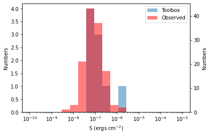
(a)

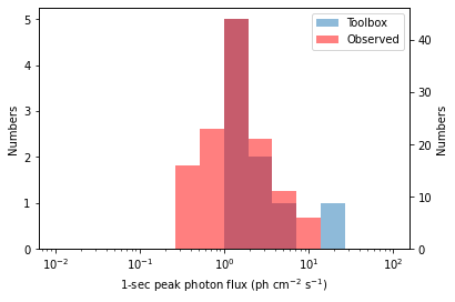
(b)

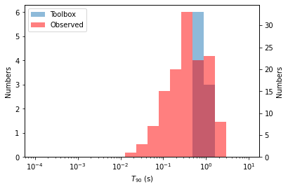
(c)

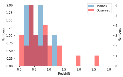
(d)

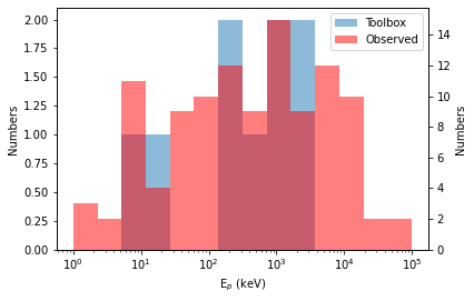
(e)

Figure 9: Fluence, 1-second peak photon flux, T90 and redshift histograms. We compare the GWToolbox simulation of Swift/BAT observing sGRBs for 1 year (blue) with all sGRBs in the Swift/BAT GRB catalogue (red) (Lien et al., 2016).

3.2 Joint detection rates

In Tab. 4, we show the number of GW detections per year for LIGO (design sensitivity) and ET, as well as joint GW-sGRB detections for four different HE detectors. We give numbers for 3 different SNR thresholds for the GW detection. In this Section, we will only discuss observations with the standard SNR of 8, whereas sub-threshold detections with SNR 7 or 6 will be addressed in Sec. 3.3. While expected joint rates for ET are in line with other predictions (e.g. Ronchini et al. (2022)), our predictions for LIGO are lower than those in other studies (e.g. Howell et al. (2019); Clark et al. (2015)). This is due to the low number of off-axis GRB observations according to our model. We further discuss this in Sec. 3.4. In Figs. 10 and 11, we visualise the redshift distribution of our predicted GW and sGRB observations, for LIGO (design sensitivity) and ET respectively. These figures do not only generally provide insights into joint detection rates, but also give information on sub-threshold and off-axis joint observations. Figs. 10-13 all use the same Fermi/GBM GRB distribution. In this Section, we will discuss the former topic of these three, whereas he latter two will be addressed in Sec. 3.3 and 3.4.

A feat that immediately stands out in Tab. 4 is the substantial difference in yearly joint detections between LIGO and ET. This is visualised in Figs. 10 and 11. To accompany these, in Fig. 12 we also show the redshift distribution of Fermi/GBM with LIGO-O3. In these figures, joint detections can only be made in the overlapping region. We see that the LIGO horizon is a main cause of the small number of joint GW-EM observations in our current era. Typical observable sGRBs by Fermi/GBM lie at redshifts $\sim$0.6-0.8, while even at design sensitivity LIGO only reaches up to redshift $\sim$0.1. For LIGO-O3, the overlap is very minimal and hardly visible. For this configuration, we expect $\sim$0.027 joint detections per year out of $\sim$0.681 GW detections per year. This is a surprisingly low number of joint observations, given that we in fact had one joint detection in O2 (Abbott et al., 2017b). We refer to Sec. 3.4 for an explanation. Even though LIGO-design shows an increase in joint detections with Fermi/GBM ($\sim$0.141 yr^-1) over LIGO-O3, drastic instrument changes would have to be made in order to significantly extend the horizon out to where more BNSs can be observed gravitationally.

Our predictions for ET show the effects of such changes, depicted in Fig. 11. Not only does ET observe significantly more sources than LIGO up to a redshift of 0.1, its horizon stretches out to much larger redshifts, clearly increasing the number of joint observations. We find that ET makes sure that the GW coverage for each HE detector in our model is close to 100%, i.e. almost every observed GRB will also have a detected GW counterpart, as the joint observation rates found in Tab. 4 are very close to the yearly detection rates by the HE instruments themselves. This is an important finding, as it will allow us to place constraints on sGRB progenitors: if all sGRBs are accompanied by a GW signal, we will know that compact binaries are the sole origins of these bursts. It is important to realise that this is a theoretical prediction, as the GW detectors do not have a 100% duty cycle, so in reality the GW coverage for every HE instument will be lower. Additionally, it should be noted that the while HE detectors that we use in the GWToolbox will not be operational during the ET era, we can still use them as reference instruments to extract useful information, some of which will apply to future instruments as well. With future HE detectors such as AMEGO (McEnery et al., 2019), HERMES (Fiore et al., 2020), TAP-GTM (Camp et al., 2019) and THESEUS (Amati et al., 2018, 2021; Ciolfi et al., 2021; Rosati et al., 2021), we will be able to make joint observations at redshifts far beyond the current Fermi/GBM limit of $\sim$2.

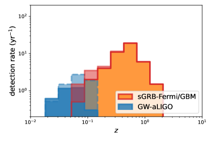
Figure 10: Redshift distribution of BNSs through detection of GWs and sGRBs. In blue, we show the distribution for LIGO (design sensitivity), where the shaded region with the dotted line represents the distribution for those GW sources with SNR between 6 and 8. In orange, we plot the distribution of Fermi/GBM GRBs (the same distribution as in Figs. 11-13), where the red region corresponds to the off-axis GRBs, generated with the addition to our model as described in Sec. 3.4.

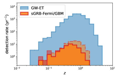
Figure 11: Redshift distribution of BNSs through detection of GWs and sGRBs. In blue, we show the distribution for ET. Again, in orange, we plot the distribution of Fermi/GBM GRBs (same distribution as Figs. 10, 12 & 13), where the red region corresponds to the off-axis GRBs, generated with the addition to our model as described in Sec. 3.4. The orange region with dotted line represents those GRBs with a peak flux between 50% and 100% of the Fermi/GBM detection threshold.

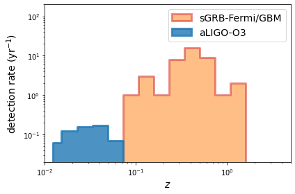
Figure 12: Redshift distribution of LIGO-O3 BNSs (blue), and Fermi/GBM BNSs measured through sGRBs (orange). Once again, the Fermi/GBM distribution is the same as in Figs. 10, 11 & 13.

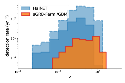
Figure 13: Redshift distribution of BNSs detected with a ”half-ET” configuration (blue) which has a sensitivity halfway between LIGO and ET, and Fermi/GBM BNSs measured through sGRBs (orange, same distribution as in Figs. 10-12). Also here, the shaded region with the dotted line corresponds to those sources with a SNR between 6 and 8. SNR8: 2038, SNR6: 6019 in 5 yrs.

For illustrative purposes, we also show a ”half-ET” configuration in of Fig. 13. This detector has a sensitivity that is halfway in-between LIGO (design sensitivity) and ET, which we obtained by multiplying the ET noise curve with a factor 10.89 (see Yi et al. (2022)), representing an early stage of the ET capability or GW detectors in-between LIGO-design and ET-design. This configuration yields $\sim$408 GW observations per year, $\sim$6 of which would be observed by Fermi/GBM as well. This shows that even an ET operating at a fraction of its capacity would be a major improvement over current-era detectors. As it is expected that ET will not immediately operate at its designed sensitivity, this is a very bright prospect. This is especially the case for the number of joint detections, as the ”half-ET” horizon lies at a redshift of $\sim$1, which is much further than the typical LIGO horizon, leading to more and higher-redshift joint detections.

3.3 Sub-threshold detections

Expected joint detection rates for different SNR thresholds
SNR	LIGO				ET
	GW	Fermi/GBM	Swift/BAT	GECAM	GW	Fermi/GBM	Swift/BAT	GECAM
8	3.330	0.141	0.0236	0.143	12470	48	7	134
7	4.792	0.178	0.0258	0.182	15372	50	8	149
6	7.033	0.252	0.0410	0.264	18951	52	8	155

Table 4: Number of GW and joint detections per year, for three different GW detector SNRs. For more accurate results, we ran all simulations involving LIGO for 1000 years rather than a single year. The numbers are the average rates from running each simulation 50 and 25 times for combinations involving LIGO and ET respectively.

Expected joint detection rates for different sub-threshold values
Sub-threshold	LIGO			ET
	Fermi/GBM	Swift/BAT	GECAM	Fermi/GBM	Swift/BAT	GECAM
1	0.141	0.0236	0.143	48	7	134
0.5	0.143	0.0239	0.145	83	12	179
0.3	0.147	0.0248	0.154	130	21	227

Table 5: Number of joint detections with different sub-threshold values for the HE detectors. Also here, we ran all simulations involving LIGO for 1000 years, and the numbers are the average rates from running each simulation 50 and 25 times for combinations involving LIGO and ET respectively.

In the multi-messenger astronomy era, we have the possibility of using GW observations to search for possible EM counterparts in data from HE instruments, as well as the other way around. Since this might lead to the discovery of sGRBs or GW signals that would otherwise not have been found, a quantitative investigation could provide us valuable insights. Here, we address the potential gains of a targeted search for sub-threshold observations of BNSs.

Tab. 4 depicts the number of GW and joint observations for different GW-HE combinations as predicted by the Toolbox, for SNR thresholds of 8, 7 and 6 respectively. With the Toolbox, we predict that for a threshold of 6, about 35 of 100 detected events is of astrophysical origin. With HE data at hand, it would be quite easy to filter out the real GW signals whose properties match with those of the detected GRBs. We find that the fraction of astrophysical events drops significantly beyond 6; at 5.5, we already find ourselves at about 1 out of 100 detections that has an astrophysical origin. However, we might be able to still pinpoint this single GW detection with sGRB data; it is generally up to the GW-EM community which lowest SNR value maximises the scientific output of such studies Lynch et al. (2018). Tab. 5 shows a type of results similar to Tab. 4, but for sub-threshold sGRB detections. Here, we do not go down further than a fraction 0.3 of the current treshold, as the Toolbox models the typical flux of the background as a fraction 0.2 of the threshold, i.e. we need to stay above the background.

Tab. 4 clearly shows that the LIGO sensitivity is an important limiting factor in the current era. Fig. 10 visualises this, as we observe that many of the sources between SNR=8 and SNR=6 are at higher redshift ($\geq$0.1, up to $\sim$0.15), beyond the LIGO horizon with SNR=8. In this case, decreasing the threshold shifts the LIGO horizon more towards the peak of the z-distribution of the HE detectors, thus increasing the number of joint detections. Decreasing the SNR to 6 would lead to an increase in joint detections of e.g. 179% and 185% for Fermi/GBM and GECAM with LIGO, respectively. As such, targeted searches for such sub-threshold GW observations would be extremely beneficial not only for the number of joint detections, but also for the BNS merger history. As the weaker GW signals typically originate from those BNSs further away, this would allow us to investigate the BNS redshift distribution and merger history in more detail. Additionally, with a larger sample extending to higher redshifts, we would be able to test gravitational waveform models in a larger part of their parameter space. Interestingly, lowering the threshold for HE detectors does not yield substantially more joint observations, as we notice in Tab. 5. While the number of sGRB detections increases for lower thresholds, the majority of them is beyond the LIGO horizon and therefore does not contribute to the joint detection rate. Only a few intrinsically faint sGRBs below redshift $\sim$0.1 are added to the number of joint detections. Therefore, we can conclude that searches for sub-threshold GRBs using LIGO detections should not be a priority. The yield of such campaigns would be very limited, and focus should be on sub-threshold GWs with information from sGRB data at hand instead.

Tabs. 4 and 5 show different patterns for the ET era. First of all, in Tab. 4 we see barely any increase in the number of joint detections as we lower the threshold and increase the number of GW observations by ET. This ties in well with our previous remarks on the fact that nearly 100% of all GRBs in the ET era will be also detected gravitationally. The depletion of current-era HE detectors during the ET era that is clearly visible here can be interpreted as a motivation for the development of new HE detectors that can keep up with the ET sensitivity. Future detectors should cover at least part of redshifts $\sim$2-5 to make a significant contribution to the number of joint detections with ET. Still, without new detectors reaching to much larger redshifts, a search for sub-threshold observations in GRB data of instuments like the current ones during the ET era could yield many new joint detections. In Tab. 5, we can see increases up to 270% for Fermi/GBM, and joint observation numbers as high as 227 per year for GECAM. Similarly to before, lowering the HE detection threshold leads to more GRBs with higher redshift, most of which have a GW counterpart. Sub-threshold searches should not only be focused on higher redshifts (beyond $\sim$2), but also on those BNSs with low inclination. Those GRBs that are further away are much more likely to be observable if their jet points in our line-of-sight; off-axis GRBs are too weak to be observed at such redshifts. BNSs with inclination angles below $\sim$15^∘ should be prioritised, as this is the typical width of a jet opening angle (Sarin et al., 2022; Fong et al., 2015; Salafia & Ghirlanda, 2022).

In Fig. 13, the shaded region around the main blue population visualises the BNS detections by the ”half-ET” configuration that have a SNR between 6 and 8. This population contains $\sim$956 BNSs per year, which results in a total number of 1364 when added to the original 408 sources with SNR $\geq$8. Most sub-threshold events are contained at redshifts beyond 0.2-0.3, reaching out to $\geq$1. The total population of BNSs with an SNR of 6 or higher yields $\sim$21 joint detections with half-ET and Fermi/GBM. This is clearly higher than the $\sim$6 joint detections for those with SNR $\geq$8. Where the redshift distribution of half-ET BNSs does not overlap completely with Fermi/GBM sGRBs, including sub-threshold GW detections can partially take care of this limitation as Fig. 13 shows us that many BNSs are added at the high-redshift end. This results in about 50% of Fermi/GBM detections that have a GW counterpart which is detectable by half-ET. Where this is clearly not close to the near 100% predicted for ET, it shows that even a half-ET configuration can be extremely beneficial and valuable for the GW-EM community, especially when compared with current-era GW instruments.

3.4 Off-axis detections

The sole joint GW-GRB detection thus far contained an off-axis GRB (Abbott et al., 2017b; Goldstein et al., 2017; Ioka & Nakamura, 2018). With the Toolbox we can predict the expected detection rate of such GRBs. We report the following results: we find $\sim$0.0035 joint observations with LIGO-O3 and Fermi/GBM per year that are off-axis (with a general joint detection rate of $\sim$0.027 yr^-1). Assuming this number is realistic, chances that the very first joint GW-sGRB observation contains an off-axis GRB are very slim, making GW170817/GRB170817A an extremely unlikely event. A more logical explanation is the fact that these numbers expose the limitations of the top-hat jet model. In reality, the energy of the GRB leaks to a wider angle than we describe in this model, leading to observable (off-axis) GRBs whose inclination is well outside the jet cone. As such, with our current model, we treat many GRBs with higher inclination angles as undetected, where in reality they are visible to HE instruments.

In this Section, we improve our off-axis detection rate by adding a second component to the model. Typically, a jet is surrounded by a wide-angle, mildly relativistic cocoon surrounding the relativistic jet (Zhang, 2018; Ciolfi, 2018). We model this cocoon as the main source of off-axis detections. Still, since the vast majority of independent HE detections of sGRBs consists of on-axis GRBs, the cocoon should be several orders of magnitude less energetic than the main jet, not significantly contributing to the HE instruments’ detection rate. We model the wide-angle cocoon emission by running a second population of GRBs, next to our main population described in Tab. 1. For this second population, we use $\log E_{\text{GRB, mean}}=48$, $\gamma=150$ and a typical $\Delta\theta_{\text{mean}}=60^{\circ}$ with $\Delta\theta_{\text{std}}=1^{\circ}$ (see e.g. Ramirez-Ruiz et al. (2002)). All other parameters remain unchanged. With this population, we can still recover the properties of GRB170817A-like GRBs, this time without having to increase $\nu^{\prime}_{0}$ to atypical values.

We show our predicted off-axis detection rates in Tab. 6. This population satisfies the condition of not significantly increasing the number of independent HE detections as compared to the main population: we find, for example, 1-2 extra detections with Fermi/GBM per year. The joint detection rates we obtain with LIGO are more in line with predictions made by previous studies (e.g. Howell et al. (2019); Clark et al. (2015)). Interestingly, we find that for all HE detectors, the joint off-axis detection rate with LIGO exceeds the number on-axis GRB observations listed in Tab. 4. Here, we can clearly see the impact of the inclination angle and redshift. With a typical cocoon opening angle about 4 times larger than the GRB jet opening angle, this second population generally contains more sources whose emission is in the line-of-sight of the detector. Moreover, even though their flux is relatively weak as compared to the main GRB jet itself, many of these GRBs are still detected due to their proximity. With the LIGO horizon at a redshift of only $\sim$0.1, a relatively high off-axis detection rate is not surprising. This shows that the properties and characteristics of GW170817/GRB170817A are not as unique as one might think at first glance; with this improvement included, an off-axis GRB as a first joint detection is in fact quite likely. For ET, the off-axis detections encompass only a small part of the total number of joint observations. When combined with the on-axis observations in Tab. 4, we still find a total rate that is in agreement with predictions (Ronchini et al., 2022). ET stretches out to a horizon (a redshift of $\sim$5) that is far beyond that of HE instruments observing off-axis GRBs (only $\sim$0.05 for Fermi/GBM). As such, the majority of ET joint observations will contain on-axis GRBs. Still, we expect more low-redshift off-axis joint detections with ET as compared to LIGO, due to its higher sensitivity. This means that the ET era is a very bright prospect, also in this regard. A potential $\sim$20 joint off-axis detections per year with ET-GECAM and likely more with next-generation HE detectors will allow us to cover significant parts of the parameter space for off-axis GRBs. We will be able to understand the GRB emission mechanism in more detail by comparing with the high number of on-axis joint detections we will have. This may probe a higher level of understanding of GRB central engines.

Expected off-axis joint detection rates
	LIGO	ET
Fermi/GBM	0.435	1.88
Swift/BAT	0.0630	0.200
GECAM	0.692	19.7

Table 6: The expected detection rates for off-axis GRBs for different GW detector - HE instrument combinations. For LIGO, we ran the population for 1000 years to obtain a more accurate rate. The values are averages that we obtained by repeating the simulation 50 times for LIGO combinations, and 25 times for ET.

4 Summary & future prospects

Based on GWToolbox, we developed an algorithm that simulates the potential prompt GRB emission from BNS and BHNS mergers, and check their detectability against a list of known HE detectors. Our algorithm pipeline of sGRB detectability determination is plotted as flowcharts in Figs. 7 and 8. We employed the algorithm to simulate observations of sGRBs and joint observations with GW and HE detectors of BNS and BHNS, and studied the prospect of sub-threshold observation strategies in both GW and HE observation.

In the list below, we summarise our main findings in this study. Afterwards, we will discuss several future prospects for additions to the model as well as possible topics to explore using the GWToolbox.

• We have constructed a sGRB model for the GWToolbox using a top-hat jet, operating with an accuracy sufficient for the purposes of the Toolbox. The addition of this model increases the number of possible uses for the Toolbox making it a valuable tool to investigate the detectability and properties of GW sources in the multi-messenger astronomy era.

• Our findings stress the significance of the impact that ET will have on multi-messenger astronomy. Where currently the LIGO sensitivity is the main limiting factor to the relatively low number of observations, we can quantitatively see that ET completely turns this around and will detect BNSs at an unprecedented rate. We have showed that a ”half-ET” instrument which is more than 10 times less sensitive than ET already increases the number of joint detections significantly.

• We find that in the ET era, the GW coverage will be close to 100% for each HE detector. Almost every detected GRB will have a GW counterpart that is observed by ET. In reality, this percentage will be lower due to the fact that GW detectors do not have a 100% duty cycle. Still, reaching 100% coverage would allow us to confirm that compact binaries are the sole origin of sGRBs.

• A targeted search campaign in LIGO data for sub-threshold GW detections has the potential of being successful in increasing the number of joint observations. LIGO is not able to detect most independent GRB detections by HE instruments. With information about the source from GRB data at hand, it will be relatively simple to pinpoint GW signals within the LIGO datastream in terms of localisation, chirp time and parameter space. We show an increase in joint detections of e.g. $\sim$185% for GECAM if we would be able to find GW detections down to an SNR of 6. This highlights the value of multi-messenger observations, as a sub-threshold search campaign will clearly increase the number of observed BNSs, as well as the parameter space in which these BNSs find themselves.

• In the ET era, this will be the other way around as we will have many more GW observations than GRB detections. Those GWs further away measured by ET can be used to search for sub-threshold GRBs. Since ET stretches quite far out, we will be able to find more (e.g. $\sim$170% more if we search down to a threshold half of the current Fermi/GBM threshold) joint detections if we perform a targeted search to sub-threshold GRBs. Such a search should be focused on high-redshift (e.g. beyond $\sim$2 for Fermi/GBM) GRBs, as closeby BNSs will be covered by both HE and GW detectors. Additionally, such campaigns are more likely to be successful when focusing on BNSs with inclinations lower than $\sim 15^{\circ}$, as this is the typical opening angle of a GRB jet.

• The top-hat jet model in the GWToolbox generally predicts joint detection rates that are quite low compared to other predictions, especially with LIGO. This is a direct result of the low number of off-axis detections predicted by the model. We achieve more realistic rates by including a second population, modelling the wide-angle cocoon around the jet, showing that the majority of joint detections in the LIGO era originates from off-axis GRBs. This feat makes the characteristics of GRB170817A not as unlikely as one may think based on the top-hat model. With ET, $\sim$100% of electromagnetically detected off-axis GRBs will have an GW counterpart. However, the ET horizon stretches far beyond the off-axis detection horizon of current HE instruments, so on-axis GRBs will dominate the ET joint detection rate.

Our model has a number of limitations that can be addressed in future work. Here, we list potential improvements that serve as future prospects for continuation of this work. Additionally, we address general applications of the newly upgraded GWToolbox now functioning as a multi-messenger simulation program.

4.1 Future improvements

• We employed the top-hat jet model in this study, and a nested wider and less energetic top-hat jet to mimic the off-axis emissions. With increasing evidences, people now believe the jet of GRB should be structured (Salafia & Ghirlanda, 2022). Our methodology is compatible with a structured jet, by substituting the top-hat function $\Pi(\Omega)$ in the emissivity with a more general continuous angular distribution. The time-evolving spectrum in this case will not take the form in equation (14), but should be integrated through equation (8) respectively.

• The comoving spectrum indices $\alpha_{B}$, $\beta_{B}$ and $s$ are not sampled from a distribution like $\gamma$, $\nu^{\prime}_{0}$ etc., but share the values for all sGRBs in the catalogue. In reality these parameters can differ from burst to burst, depending on the local emission condition and mechanism. We argue that the influence on detectability of bursts from the diversity on these spectrum parameters is largely degenerate with that from $\gamma$ and $\nu^{\prime}_{0}$. Our current treatment is a trade-off between the generality and degrees-of-freedom of the model, although extension to include six more hyper-parameters to describing distributions of these spectrum parameters would be straightforward. Other possible improvements to the spectrum could be more along the lines of Ioka & Nakamura (2019), where we would implement an intrinsic angular dependence in both $\gamma$ and $\nu^{\prime}_{0}$.

• In our simulation, we assume every BNS merger or BHNS that have $R_{\text{t}}>R_{\text{ISCO}}$ is associated with prompt GRB emission. While there are studies show that some merger remnants can not work as engine to power a GRB jet (Sarin & Lasky, 2020; Shemi & Piran, 1990; Ciolfi, 2018; Nakar, 2007; Murguia-Berthier et al., 2014, 2017; Margalit et al., 2015; Beniamini et al., 2017), and the scenario of a ”choked jet” is also possible; here, the jet fails to break out of the surrounding ejecta, and is not able to dissipate and emit a prompt GRB (Rosswog & Davies, 2002; Murguia-Berthier et al., 2014; Lazzati et al., 2018; Bromberg et al., 2011; Lazzati & Perna, 2019; Salafia et al., 2020). The above mentioned possibility will yield a fraction of failed GRB, which is not considered in our treatment, and will cause an overestimation of the sGRB detection rate by a factor $f_{\text{fail}}$; On the other hand, there could be sGRB whose progenitor is other than BNS/BHNS merger, which we also did not include in our consideration, which will cause an underestimation of the detection rate by a factor $f_{\text{other}}$. Since we collaborate the simulator with the historical detection rates, those effect of $f_{\text{other}}f_{\text{fail}}$ is absorbed into the merger rate parameter $R_{\text{n}}$ and the detector correcting factor $f_{c}$, and therefore will not cause under- or overestimation on the detection rate of future (joint) observations. When $R_{\text{n}}$ is more accurately estimated from a larger GW population, and $f_{c}$ is determined through dedicated trigger simulations, $f_{\text{fail}}f_{\text{other}}$ will be in turn constrained.

4.2 Applications on GRB physics and compact binaries merger history

As shown inTab. 1, the underlying GRB population model of the simulator has hyper-parameters that describe the merger rate of the progenitor binaries and GRB physics. A comparison between the simulated catalogue with the real observation from the same detector can in turn give constraints on this parameters, and thus give information on the GRB physics and progenitor binaries merger history. More specifically, such inference can be done in a Bayesian fashion:

$$p(\mathcal{B}|\{\Theta_{i}\})\propto\mathcal{L}(\{\Theta_{i}\}|\mathcal{B})p(\mathcal{B}),$$ (22)

where $p(\mathcal{B}|\{\Theta_{i}\})$ is the posterior distributions of the list of the hyper-parameters of GRB population model, given a catalogue of detected GRB $\{\Theta_{i}\}$. $\Theta_{i}$ denotes a list of observable, e.g.,T90, Fluence, redshift, $E_{\rm{peak}}$ etc., of the $i$-th sGRB in the catalogues.

The key step is to find out the likelihood function on the right-hand side: $\mathcal{L}(\{\Theta_{i}\}|\mathcal{B})$, which has a known function form as in a inhomogeneous Poisson process:

$$\mathcal{L}(\{\Theta_{i}\}|\mathcal{B})=N!\prod_{i=1}^{N}p(\Theta_{i,\rm{obs}}|\mathcal{B})p(N|\lambda_{\rm{GRB}}(\mathcal{B})),$$ (23)

where $N$ is the number of event in the catalogue, $z_{i}$ is the redshift of $i$-th sGRB, $p(z_{i,\rm{obs}}|\mathcal{B})$ is probability of observing $z_{i}$ given model, and $\lambda_{\rm{GRB}}$ is the expected total number in the catalogue, which is also function of model parameters $\mathcal{B}$. $p(N|\lambda_{GRB})$ is a Poisson probability with expectation $\lambda_{\rm{GRB}}$. With simulations from GWToolbox, $\lambda_{GRB}$ and $p(\Theta_{i,\rm{obs}}|\mathcal{B})$ can be obtained, and thus makes the study possible.

References

- Abbott et al. (2017a) Abbott, B., Abbott, R., Abbott, T., et al. 2017a, Physical Review Letters, 119, 161101
- Abbott et al. (2020) Abbott, B. P., Abbott, R., Abbott, T. D., et al. 2020, The Astrophysical Journal Letters, 892, L3
- Abbott et al. (2017b) Abbott, B. P., Abbott, R., Abbott, T. D., et al. 2017b, The Astrophysical Journal, 848, L12
- Abbott et al. (2021a) Abbott, R., Abbott, T. D., Abraham, S., et al. 2021a, The Astrophysical Journal Letters, 915, L5
- Abbott et al. (2021b) Abbott, R., Abbott, T. D., Abraham, S., et al. 2021b, The Astrophysical Journal Letters, 913, L7
- Acernese et al. (2015) Acernese, F., Agathos, M., Agatsuma, K., et al. 2015, Classical and Quantum Gravity, 32, 024001
- Amati et al. (2021) Amati, L., O’Brien, P. T., Götz, D., Bozzo, E., & Santangelo, A. 2021, The THESEUS space mission: updated design, profile and expected performances, Tech. rep., publication Title: arXiv e-prints ADS Bibcode: 2021arXiv210208702A Type: article
- Amati et al. (2018) Amati, L., O’Brien, P., Götz, D., et al. 2018, Advances in Space Research, 62, 191
- Band et al. (1993) Band, D., Matteson, J., Ford, L., et al. 1993, The Astrophysical Journal, 413, 281
- Barthelmy et al. (2005) Barthelmy, S. D., Barbier, L. M., Cummings, J. R., et al. 2005, Space Science Reviews, 120, 143
- Beniamini et al. (2017) Beniamini, P., Giannios, D., & Metzger, B. D. 2017, Monthly Notices of the Royal Astronomical Society, 472, 3058
- Bernuzzi (2020) Bernuzzi, S. 2020, General Relativity and Gravitation, 52, 108
- Bernuzzi et al. (2020) Bernuzzi, S., Breschi, M., Daszuta, B., et al. 2020, Monthly Notices of the Royal Astronomical Society, 497, 1488
- Bhat et al. (2016) Bhat, P. N., Meegan, C. A., von Kienlin, A., et al. 2016, The Astrophysical Journal Supplement Series, 223, 28
- Bromberg et al. (2011) Bromberg, O., Nakar, E., Piran, T., & Sari, R. 2011, The Astrophysical Journal, 740, 100, aDS Bibcode: 2011ApJ…740..100B
- Brown et al. (2020) Brown, D. D., Jones, P., Rowlinson, S., et al. 2020, SoftwareX, 12, 100613
- Camp et al. (2019) Camp, J., Abel, J., Barthelmy, S., et al. 2019, 51, 85, conference Name: Bulletin of the American Astronomical Society ADS Bibcode: 2019BAAS…51g..85C
- Chen et al. (2021a) Chen, H.-Y., Cowperthwaite, P. S., Metzger, B. D., & Berger, E. 2021a, The Astrophysical Journal, 908, L4
- Chen et al. (2021b) Chen, H.-Y., Holz, D. E., Miller, J., et al. 2021b, Classical and Quantum Gravity, 38, 055010, arXiv:1709.08079 [astro-ph]
- Ciolfi (2018) Ciolfi, R. 2018, International Journal of Modern Physics D, 27, 1842004, arXiv: 1804.03684
- Ciolfi et al. (2021) Ciolfi, R., Stratta, G., Branchesi, M., et al. 2021, Experimental Astronomy, 52, 245
- Clark et al. (2015) Clark, J., Evans, H., Fairhurst, S., et al. 2015, The Astrophysical Journal, 809, 53
- Coward et al. (2012) Coward, D., Howell, E., Piran, T., et al. 2012, Monthly Notices of the Royal Astronomical Society, 425, 2668, arXiv: 1202.2179
- Eichler et al. (1989) Eichler, D., Livio, M., Piran, T., & Schramm, D. N. 1989, Nature, 340, 126
- Fiore et al. (2020) Fiore, F., Burderi, L., Lavagna, M., et al. 2020, in Space Telescopes and Instrumentation 2020: Ultraviolet to Gamma Ray, ed. J.-W. A. den Herder, K. Nakazawa, & S. Nikzad (Online Only, United States: SPIE), 166
- Fong et al. (2015) Fong, W., Berger, E., Margutti, R., & Zauderer, B. A. 2015, The Astrophysical Journal, 815, 102
- Frail et al. (2001) Frail, D. A., Kulkarni, S. R., Sari, R., et al. 2001, The Astrophysical Journal, 562, L55
- Fryer et al. (2015) Fryer, C. L., Belczynski, K., Ramirez-Ruiz, E., et al. 2015, The Astrophysical Journal, 812, 24
- Gehrels et al. (2004) Gehrels, N., Chincarini, G., Giommi, P., et al. 2004, The Astrophysical Journal, 611, 1005
- Goldstein et al. (2017) Goldstein, A., Veres, P., Burns, E., et al. 2017, The Astrophysical Journal, 848, L14
- Gruber et al. (2014) Gruber, D., Goldstein, A., von Ahlefeld, V. W., et al. 2014, The Astrophysical Journal Supplement Series, 211, 12
- Harry & the LIGO Scientific Collaboration (2010) Harry, G. M. & the LIGO Scientific Collaboration. 2010, Classical and Quantum Gravity, 27, 084006
- Howell et al. (2019) Howell, E. J., Ackley, K., Rowlinson, A., & Coward, D. 2019, Monthly Notices of the Royal Astronomical Society, 485, 1435
- Husa et al. (2016) Husa, S., Khan, S., Hannam, M., et al. 2016, Physical Review D, 93, 044006, arXiv:1508.07250 [gr-qc]
- Ioka & Nakamura (2001) Ioka, K. & Nakamura, T. 2001, The Astrophysical Journal, 554, L163
- Ioka & Nakamura (2018) Ioka, K. & Nakamura, T. 2018, arXiv:1710.05905 [astro-ph, physics:gr-qc], arXiv: 1710.05905
- Ioka & Nakamura (2019) Ioka, K. & Nakamura, T. 2019, Monthly Notices of the Royal Astronomical Society, 487, 4884
- Khan et al. (2016) Khan, S., Husa, S., Hannam, M., et al. 2016, Physical Review D, 93, 044007, arXiv:1508.07253 [gr-qc]
- Kim (2021) Kim, C. 2021, Journal of the Korean Physical Society, 78, 918
- Lazzati & Perna (2019) Lazzati, D. & Perna, R. 2019, The Astrophysical Journal, 881, 89, aDS Bibcode: 2019ApJ…881…89L
- Lazzati et al. (2018) Lazzati, D., Perna, R., Morsony, B. J., et al. 2018, Physical Review Letters, 120, 241103
- Lien et al. (2016) Lien, A., Sakamoto, T., Barthelmy, S. D., et al. 2016, The Astrophysical Journal, 829, 7, arXiv:1606.01956 [astro-ph]
- Lynch et al. (2018) Lynch, R., Coughlin, M., Vitale, S., Stubbs, C. W., & Katsavounidis, E. 2018, The Astrophysical Journal, 861, L24
- Margalit et al. (2015) Margalit, B., Metzger, B. D., & Beloborodov, A. M. 2015, Physical Review Letters, 115, 171101
- McEnery et al. (2019) McEnery, J., Barrio, J. A., Agudo, I., et al. 2019, arXiv:1907.07558 [astro-ph]
- Meegan et al. (2009) Meegan, C., Lichti, G., Bhat, P. N., et al. 2009, The Astrophysical Journal, 702, 791
- Metzger (2019) Metzger, B. D. 2019, Annals of Physics, 410, 167923
- Murguia-Berthier et al. (2014) Murguia-Berthier, A., Montes, G., Ramirez-Ruiz, E., De Colle, F., & Lee, W. H. 2014, The Astrophysical Journal, 788, L8
- Murguia-Berthier et al. (2017) Murguia-Berthier, A., Ramirez-Ruiz, E., Montes, G., et al. 2017, The Astrophysical Journal, 835, L34
- Müller & Serot (1996) Müller, H. & Serot, B. D. 1996, Nuclear Physics A, 606, 508
- Müther et al. (1987) Müther, H., Prakash, M., & Ainsworth, T. 1987, Physics Letters B, 199, 469
- Nakar (2007) Nakar, E. 2007, Physics Reports, 442, 166
- Nedora et al. (2020) Nedora, V., Schianchi, F., Bernuzzi, S., et al. 2020, arXiv:2011.11110 [astro-ph, physics:gr-qc], arXiv: 2011.11110
- Piran (1999) Piran, T. 1999, Physics Reports, 314, 575
- Prakash et al. (1988) Prakash, M., Ainsworth, T. L., & Lattimer, J. M. 1988, Physical Review Letters, 61, 2518
- Preece et al. (2000) Preece, R. D., Briggs, M. S., Mallozzi, R. S., et al. 2000, The Astrophysical Journal Supplement Series, 126, 19, aDS Bibcode: 2000ApJS..126…19P
- Punturo et al. (2010) Punturo, M., Abernathy, M., Acernese, F., et al. 2010, Classical and Quantum Gravity, 27, 194002
- Radice et al. (2018) Radice, D., Perego, A., Hotokezaka, K., et al. 2018, The Astrophysical Journal, 869, 130
- Ramirez-Ruiz et al. (2002) Ramirez-Ruiz, E., Celotti, A., & Rees, M. J. 2002, Monthly Notices of the Royal Astronomical Society, 337, 1349, arXiv:astro-ph/0205108
- Reitze et al. (2019) Reitze, D., Adhikari, R. X., Ballmer, S., et al. 2019, number: arXiv:1907.04833 arXiv:1907.04833 [astro-ph, physics:gr-qc]
- Ronchini et al. (2022) Ronchini, S., Branchesi, M., Oganesyan, G., et al. 2022, number: arXiv:2204.01746 arXiv:2204.01746 [astro-ph, physics:gr-qc]
- Rosati et al. (2021) Rosati, P., Basa, S., Blain, A. W., et al. 2021, Experimental Astronomy, 52, 407
- Rosswog & Davies (2002) Rosswog, S. & Davies, M. B. 2002, Monthly Notices of the Royal Astronomical Society, 334, 481
- Salafia et al. (2020) Salafia, O. S., Barbieri, C., Ascenzi, S., & Toffano, M. 2020, Astronomy & Astrophysics, 636, A105
- Salafia & Ghirlanda (2022) Salafia, O. S. & Ghirlanda, G. 2022, arXiv:2206.11088 [astro-ph]
- Sarin & Lasky (2020) Sarin, N. & Lasky, P. D. 2020, arXiv:2012.08172 [astro-ph, physics:gr-qc], arXiv: 2012.08172
- Sarin et al. (2022) Sarin, N., Lasky, P. D., Vivanco, F. H., et al. 2022, arXiv:2201.08491 [astro-ph, physics:gr-qc], arXiv: 2201.08491
- Shemi & Piran (1990) Shemi, A. & Piran, T. 1990, The Astrophysical Journal, 365, L55, aDS Bibcode: 1990ApJ…365L..55S
- Song et al. (2022) Song, X.-Y., Xiong, S.-L., Zhang, S.-N., et al. 2022, The Astrophysical Journal Supplement Series, 259, 46
- von Kienlin et al. (2014) von Kienlin, A., Meegan, C. A., Paciesas, W. S., et al. 2014, arXiv:1401.5080 [astro-ph]
- von Kienlin et al. (2020) von Kienlin, A., Meegan, C. A., Paciesas, W. S., et al. 2020, The Astrophysical Journal, 893, 46
- Woods & Loeb (1999) Woods, E. & Loeb, A. 1999, The Astrophysical Journal, 523, 187
- Xiao et al. (2022) Xiao, S., Liu, Y. Q., Peng, W. X., et al. 2022, Monthly Notices of the Royal Astronomical Society, 511, 964
- Yi et al. (2021) Yi, S.-X., Nelemans, G., Brinkerink, C., et al. 2021, arXiv:2106.13662 [astro-ph], arXiv: 2106.13662
- Yi et al. (2022) Yi, S.-X., Stoppa, F., Nelemans, G., & Cator, E. 2022, Astronomy & Astrophysics
- Zhang (2018) Zhang, B. 2018, The physics of gamma-ray bursts (Cambridge ; New York, NY: Cambridge University Press)
- Zhang et al. (2019) Zhang, D., Li, X., Xiong, S., et al. 2019, Nuclear Instruments and Methods in Physics Research Section A: Accelerators, Spectrometers, Detectors and Associated Equipment, 921, 8