Identifying Weight-Variant Latent Causal Models

Abstract

The task of causal representation learning aims to uncover latent higher-level causal representations that affect lower-level observations. Identifying true latent causal representations from observed data, while allowing instantaneous causal relations among latent variables, remains a challenge, however. To this end, we start with the analysis of three intrinsic indeterminacies in identifying latent space from observations: transitivity, permutation indeterminacy, and scaling indeterminacy. We find that transitivity acts as a key role in impeding the identifiability of latent causal representations. To address the unidentifiable issue due to transitivity, we introduce a novel identifiability condition where the underlying latent causal model satisfies a linear-Gaussian model, in which the causal coefficients and the distribution of Gaussian noise are modulated by an additional observed variable. Under some mild assumptions, we can show that the latent causal representations can be identified up to trivial permutation and scaling. Furthermore, based on this theoretical result, we propose a novel method, termed Structural caUsAl Variational autoEncoder (SuaVE), which directly learns latent causal representations and causal relationships among them, together with the mapping from the latent causal variables to the observed ones. Experimental results on synthetic and real data demonstrate the identifiability and consistency results and the efficacy of SuaVE in learning latent causal representations.

1 Introduction

While there is no universal formal definition, one widely accepted feature of disentangled representations (Bengio et al., 2013) is that a change in one dimension corresponds to a change in one factor of variation in the underlying model of the data, while having little effect on others. The underlying model is rarely available for interrogation, however, which makes learning disentangled representations challenging. Several excellent works for disentangled representation have been proposed that focus on enforcing independence over the latent variables that control the factors of variation (Higgins et al., 2017; Chen et al., 2018; Locatello et al., 2019; Kim & Mnih, 2018; Locatello et al., 2020). In many applications, however, the latent variables are not statistically independent, which is at odds with the notion of disentanglement, i.e., foot length and body height exhibit strong correlation in the observed data (Träuble et al., 2021).

Causal representation learning avoids the aforementioned limitation, as it aims to learn a representation that exposes the unknown high-level causal structural variables, and the relationships between them, from a set of low-level observations (Schölkopf et al., 2021). Unlike disentangled representation learning, it identifies the possible causal relations among latent variables. In fact, disentangled representation learning can be viewed as a special case of causal representation learning where the latent variables have no causal influences (Schölkopf et al., 2021). One of the most prominent additional capabilities of causal representations is the ability to represent interventions and to make predictions regarding such interventions (Pearl, 2000), which enables the generation of new samples that do not lie within the distribution of the observed data. This can be particularly useful to improve the generalization of the resulting model. Causal representations also enable answering counterfactual questions, e.g., would a given patient have suffered heart failure if they had started exercising a year earlier?

Despite its advantages, causal representation learning is a notoriously hard problem—without certain assumptions, identifying the true latent causal model from observed data is generally not possible. There are three primary approaches to achieve identifiability: 1) adapting (weakly) supervised methods with given latent causal graphs or/and labels (Kocaoglu et al., 2018; Yang et al., 2021; Von Kügelgen et al., 2021; Brehmer et al., 2022), 2) imposing sparse graphical conditions, e.g., with bottleneck graphical conditions (Adams et al., 2021; Xie et al., 2020; Lachapelle et al., 2021), 3) using temporal information (Yao et al., 2021; Lippe et al., 2022). A brief review is provided in Section 2. For the supervised approach, when labels are known, the challenging identifiability problem in latent space has been transferred to an identifiability problem in the observed space, for which some commonly-used functional classes have been proven to be identifiable (Zhang & Hyvarinen, 2012; Peters et al., 2014). Given latent causal graphs overly depends on domain knowledge. For the second approach, many true latent causal graphs do not satisfy the assumed sparse graph structure. The temporal approach is only applicable when temporal information or temporal intervened information among latent factors is available.

In this work, we explore a new direction in the identifiability of latent causal representations, by allowing causal influences among latent causal variables to change, motivated by recent advances in nonlinear ICA (Hyvarinen et al., 2019; Khemakhem et al., 2020). Hyvarinen et al. (2019); Khemakhem et al. (2020) have shown that with an additional observed variable $\mathbf{u}$ to modulate latent independent variables, the latent independent variables conditional on $\mathbf{u}$ are identifiable. Then a question naturally arises: with causal relationships among latent variables, what additional assumptions are required for the identifiability? To answer this question, we start from the analysis of three intrinsic indeterminacies in latent space (see Section 3): transitivity, permutation indeterminacy, and scaling indeterminacy, which further give rise to the following insights. 1) Transitivity is the scourge of identifiability of the latent causal model. 2) Permutation indeterminacy means the recovered latent variables can have an arbitrary permutation of the underlying orders, due to the flexibility in latent space. This nature enables us to enforce the learned causal representations in correct causal orders regularized by a predefined a directed acyclic fully-connected graph, avoiding troublesome directed acyclic graph (DAG) constraints. 3) Scaling and permutation indeterminacy only allow recovering latent causal variables up to permutation and scaling, not the exact values. To overcome the transitivity challenge we model the underlying causal representation with weight-variate linear Gaussian models, where both the weights (i.e., causal coefficients) and the mean and variance of the Gaussian noise are modulated by an additional observed variable $\mathbf{u}$ (see Section 4). With these assumptions, we can show that the latent causal representations can be recovered up to a trivial permutation and scaling. Based on this result, in Section 5, we further propose a novel method, Structural caUsAl Variational autoEncoder (SuaVE), for learning latent causal representations with consistency guarantee. Section 6 verifies the efficacy of the proposed approach on both synthetic and real fMRI data.

The key to the identifiability result above is that the causal influences (weights) among the latent causal variables are allowed to change. Intuitively, the changing causal influences enable us to obtain (soft) interventional observed data, which enables the identifiability of the latent causal variables. In fact, the change of causal influences for identifiability has been explored in observed space (Ghassami et al., 2018; Huang* et al., 2020). In addition, recent progress in identifying latent causal representation by randomly chosen unknown hard intervention Brehmer et al. (2022) can be regarded as a special change of causal influences.

2 Related work

Due to the challenges of identifiability in causal representation learning, most existing works handle this problem by imposing assumptions. We thus give a brief review of the related work on this basis.

(Weakly) Supervised Causal Representation Learning Approaches falling within this class assume known latent causal graphs or labels. CausalGAN (Kocaoglu et al., 2018) requires a-priori knowledge of the structure of the causal graph of latent variables, which is a significant practical limitation. CausalVAE (Yang et al., 2021) needs additional labels to supervise the learning of latent variables. Such labels are not commonly available, however, and manual labeling can be costly and error-prone. Von Kügelgen et al. (2021) use a known but non-trivial causal graph between content and style factors to study self-supervised causal representation learning. Brehmer et al. (2022) learn causal representation in a weakly supervised setting whereby they assume access to data pairs representing the system before and after a randomly chosen unknown intervention.

Sparse Graphical Structure  Most recent progress in identifiability focuses on sparse graphical structure constraints (Silva et al., 2006; Shimizu et al., 2009; Anandkumar et al., 2013; Frot et al., 2019; Cai et al., 2019; Xie et al., 2020, 2022). Adams et al. (2021) provided a unifying viewpoint of this approach whereby a sparser model that fits the observation is preferred. However, they primarily consider linear relations between latent causal variables, and between latent causal variables and observed variables, which are often violated in real-world applications. Lachapelle et al. (2021) handles nonlinear causal relation between latent variables by assuming special sparse graphical structures. However, many latent causal graphs in reality may be more or less arbitrary, beyond a purely sparse graph structure. In contrast, our work assumes a function class of latent variables, and does not restrict the graph structure over them.

Temporal Information  The temporal constraint that the effect cannot precede the cause has been used repeatedly in latent causal representation learning (Yao et al., 2021; Lippe et al., 2022; Yao et al., 2022). For example, Yao et al. (2021) recover latent causal variables and the relations between them using Variational AutoEncoders and enforcing constraints in causal process prior. Lippe et al. (2022) learn causal representations from temporal sequences, which requires the underlying causal factors to be intervened. All of these works can be regarded as special cases of exploring the change of causal influences among latent variables in time series data. The approach proposed is more general since the observed auxiliary variable $\mathbf{u}$ could represent time indices, domain indices, or almost any additional or side information.

Besides, Kivva et al. (2021) considers a nonlinear setting for latent causal discovery. It assumes discrete latent causal variables that are rendered identifiable by a mixture oracle, while here we consider continuous latent causal variables.

3 Indeterminacies in Latent Causal Models

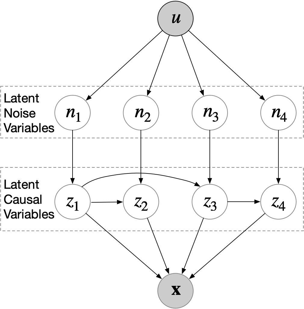
Figure 1: Causal representation with $\mathbf{u}$.

In this section, we first build a connection between nonlinear ICA and causal representation learning, by exploiting the correspondence between the independence of latent variables in nonlinear ICA and the independence of latent noise variables in causal representations. We then consider three indeterminacies in latent space: transitivity, permutation indeterminacy, and scaling indeterminacy, and analyze their impact on identifiability.

3.1 Relating Causal Representation with Identifiable Nonlinear ICA

Causal representation learning aims to uncover latent higher-level causal representations that can explain lower-level raw observations with a nonlinear mapping. Specifically, we assume that the observed variables $\mathbf{x}$ are influenced by latent causal variables ${z_{i}}$, and the causal structure among ${z_{i}}$ can be any directed acyclic graph (which is unknown). For each latent causal variable $z_{i}$, there is a corresponding latent noise variable $n_{i}$, as shown in Figure 1, which represents some unmeasured factors that influence $z_{i}$. The latent noise variables $n_{i}$ are assumed to be independent with each other, conditional on the observed variable $\mathbf{u}$, in a causal system (Peters et al., 2017), so it is natural to leverage recent progress in nonlinear ICA (Hyvarinen et al., 2019; Khemakhem et al., 2020), which has shown that the independent latent noise variables $n_{i}$ are identifiable under relatively mild assumptions, i.e., one of the main assumptions is that $\{n_{i}\}$ are Gaussian distributed with their mean and variance modulated by an observed variable $\mathbf{u}$. Taking one step further, our goal is to recover the latent causal variables $z_{i}$. However, with the assumptions for the identifiability of latent noise variables $n_{i}$ from nonlinear ICA, it is still insufficient to identify the latent causal variables $z_{i}$. The reason of such non-identifiability will be given in Section 3.2. Given this fact, a further question is what additional conditions are needed to recover the latent causal variables $z_{i}$. The corresponding identifiability conditions will be given in Section 4.

3.2 Transitivity: the Challenge of Identifying Causal Representations

Even with the identifiable $n_{i}$, it is impossible to identify the latent causal variables $z_{i}$ without additional assumptions. To interpret this point, for simplicity, let us only consider the influences of $z_{1}$ and $z_{2}$ on $\mathbf{x}$ in Figure 1. According to the graph structure in Figure 1, assume that $z_{1}:=n_{1}$, $z_{2}:=z_{1}+n_{2}$ and $\mathbf{x}:=\mathbf{f}(z_{1},z_{2})+{\boldsymbol{\varepsilon}}$ (case 1). We then consider the graph structure shown in the left column of Figure 2, where the edge $z_{1}\rightarrow z_{2}$ has been removed, and assume that $z_{1}:=n_{1}$, $z_{2}:=n_{2}$ and $\mathbf{x}:=\mathbf{f}\circ\mathbf{g}(z_{1},z_{2})+{\boldsymbol{\varepsilon}}$ where $\mathbf{g}(z_{1},z_{2})=[z_{1},z_{1}+z_{2}]$ (case 2). Interestingly, we find that the causal models in case 1 and case 2 generate the same observed data $\mathbf{x}$, which implies that there are two different causal models to interpret the same observed data. Clearly, $z_{2}$ in both the two equivalent causal structures are different, and thus $z_{2}$ is unidentifiable.

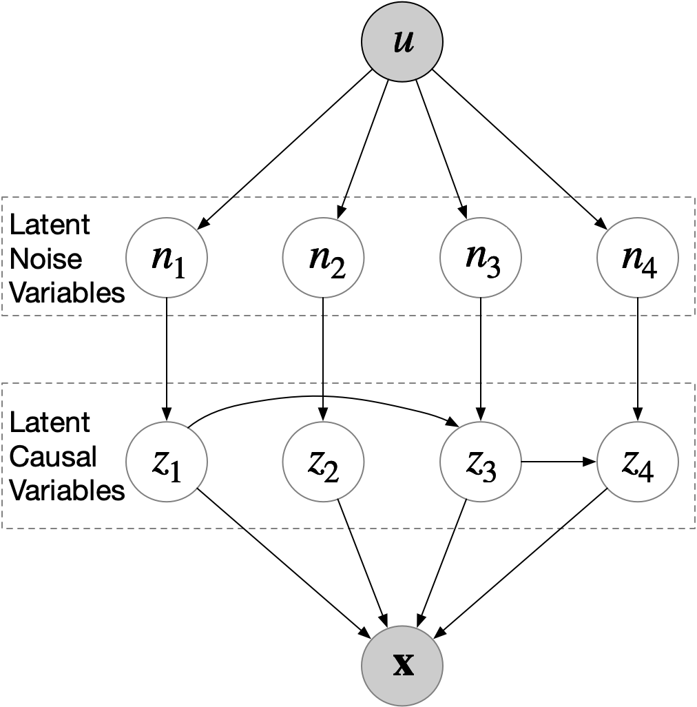
Figure 2: Two equivalent graph structures.

Similarly, we can cut the edge $z_{1}\rightarrow z_{3}$ in Figure 1, obtaining another equivalent causal graph as shown in the right of Figure 2. That is, we can have two different $z_{3}$ to interpret the same observed data, and thus $z_{3}$ is unidentifiable. Since there exist many different equivalent causal structures, the latent causal variables in Figure 1 are unidentifiable. Such a result is because the effect of $z_{1}$ on $z_{2}$ (or $z_{3}$) in latent space can be ‘absorbed’ by the nonlinear function from $\mathbf{z}$ to $\mathbf{x}$. We term this indeterminacy transitivity in this work. We will show how to handle this challenge in Section 4. Before that, we introduce the other two indeterminacies in latent space, which assists in understanding our identifiability result.

3.3 Scaling Indeterminacy in Causal Representations

The scaling indeterminacy of latent causal variables is also an intrinsic indeterminacy in latent space. Again, for simplicity, we only consider the influence of $z_{1}$ and $z_{2}$ on $\mathbf{x}$ in Figure 1, and assume that $z_{1}:=n_{1}$, $z_{2}:=z_{1}+n_{2}$ and $\mathbf{x}:=\mathbf{f}(z_{1},z_{2})+{\boldsymbol{\varepsilon}}$. Under this setting, if the value of $z_{1}$ is scaled by $s$, e.g. $s\times z_{1}$, we can easily obtain the same observed data $\mathbf{x}$ by: 1) letting $z_{2}:=\frac{1}{s}\times z_{1}+n_{2}$ and 2) $\mathbf{x}:=\mathbf{f}\circ\mathbf{g}(z_{1},z_{2})+{\boldsymbol{\varepsilon}}$ where $\mathbf{g}(z_{1},z_{2})=[s\times z_{1},z_{1}]$. This indeterminacy is because the scaling of the latent variables $z_{i}$ can be ‘absorbed’ by the nonlinear function from $\mathbf{z}$ to $\mathbf{x}$ and the causal functions among the latent causal variables. Therefore, without additional information to determine the values of the latent causal variables $z_{i}$, it is only possible to identify the latent causal variable up to scaling, not exactly recovering the values. In general, this scaling does not affect identifying the causal structure among the latent causal variables. We will further discuss this point in Section 4.

3.4 Permutation Indeterminacy in Causal Representations

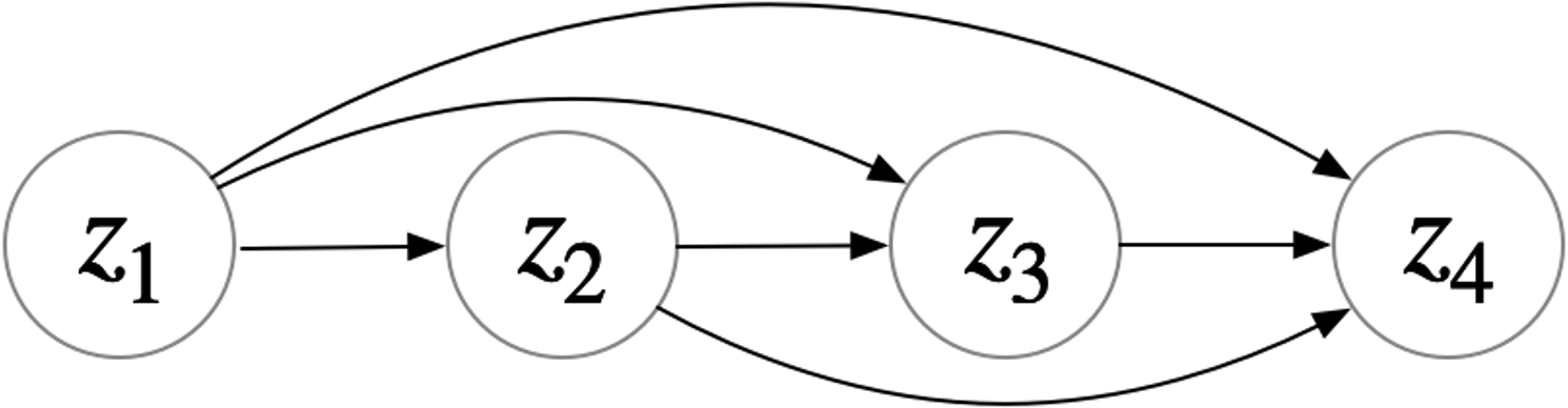
Figure 3: A Causal Fully-connected Graph.

Due to the nature of ill-posedness, latent causal representation learning suffers from permutation indeterminacy, where the recovered latent causal representations have an arbitrary permutation. For example, assume that the underlying (synthetic) latent causal representations are corresponding to the size, color, shape, and location of an object, and we obtain the recovered latent causal representations $z_{1},z_{2},z_{3},z_{4}$. Permutation indeterminacy means that we can not ensure that the recovered $z_{1}$ represents which specified semantic information, e.g., the size or the color. Therefore, without additional information to determine the order of the recovered latent causal representations $z_{i}$, it is only possible to identify the latent causal representations up to permutation.

Although the flexibility and ambiguity in latent space cause permutation indeterminacy bringing some troubles, they also bring a benefit for learning latent causal representations with a straightforward way to handle the causal order on latent causal representations. That is, we can always pre-define a causal order $z_{1},z_{2},z_{3},z_{4}$, without specified semantic information for the nodes. Based on this, we can further pre-define a causal fully-connected graph as depicted by Figure 3. As a result, the four predefined nodes $z_{1},z_{2},z_{3},z_{4}$ are enforced to learn four corresponding latent variables in the correct causal order. For example, assume that a correct underlying causal order is: size $\succ$ color $\succ$ shape $\succ$ location. Since $z_{1}$ is the first node in the predefined causal fully-connected graph, $z_{1}$ is enforced to the semantic information of the first node in the correct underlying causal order, e.g., the size. Similarly, $z_{2}$ is enforced to the semantic information of the second node in the correct underlying causal order, e.g., the color. The proposed causal fully-connected graph can naturally ensure a directed acyclic graph estimation in learning causal representation, avoiding DAG constraints (such as the one proposed in Zheng et al. (2018)). We will further show how to implement it in the proposed method in Section 5.

4 Identifiable Causal Representations with Weight-variant Linear Gaussian Models

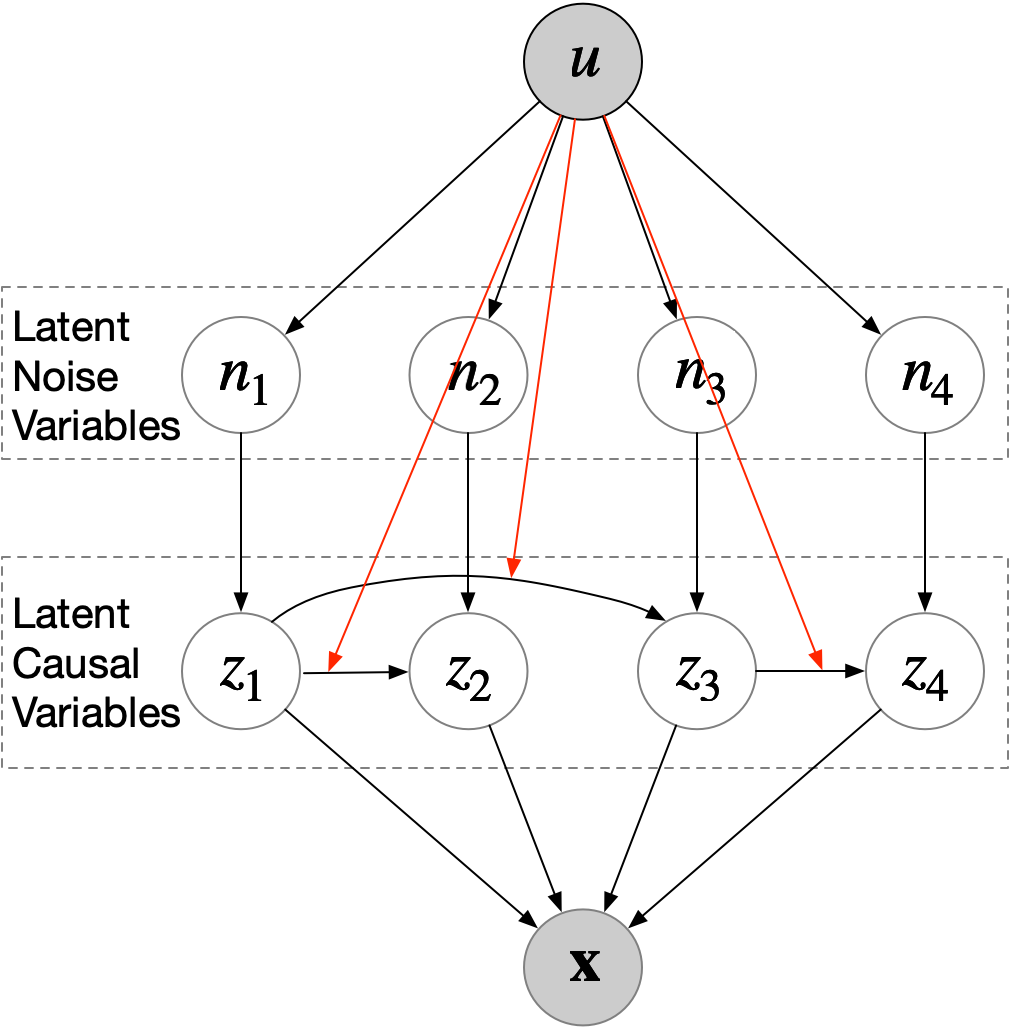
Figure 4: The proposed Latent Causal Model. Here we use the ’red’ lines to indicate the changes of weights across $\mathbf{u}$, which is different from the definition of edges (e.g., causal direction) in standard SCM.

As discussed in Section 3.2, the key factor that impedes identifiable causal representations is the transitivity in latent space. Note that the transitivity is because the causal influences among the latent causal variables may be ‘absorbed’ by the nonlinear mapping from latent variables $\mathbf{z}$ to the observed variable $\mathbf{x}$. To address this issue, motivated by identifying causal structures with the change of causal influences in observed space (Ghassami et al., 2018; Huang et al., 2019; Huang* et al., 2020), we allow causal influences among latent causal variables to be modulated by an additionally observed variable $\mathbf{u}$, represented by the red edge in Figure 4. Intuitively, variant causal influences among latent causal variables cannot be ‘absorbed’ by an invariant nonlinear mapping from $\mathbf{z}$ to $\mathbf{x}$, resulting in identifiable causal representations. We assume $\mathbf{x}$ and $\mathbf{z}$ satisfy:

$$n_{i}:\sim{\cal N}({\beta_{i,1}(\mathbf{u})},{\beta_{i,2}(\mathbf{u})}),$$ (1)

$${z_{i}}:={\boldsymbol{\lambda}^{T}_{i}(\mathbf{u})(\mathbf{z})}+n_{i},$$ (2)

$$\mathbf{x}:=\mathbf{f}(\mathbf{z})+\boldsymbol{\varepsilon}$$ (3)

where

• each noise term $n_{i}$ is Gaussian distributed with mean ${\beta_{i,1}(\mathbf{u})}$ and variance ${\beta_{i,2}(\mathbf{u})}$; both ${\beta_{i,1}}$ and ${\beta_{i,2}}$ can be nonlinear mappings. Moreover, the distribution of $n_{i}$ is modulated by the observed variable $\mathbf{u}$.

• In Eq. (2), $\boldsymbol{\lambda_{i}}(\mathbf{u})$ denote the vector corresponding to the causal weights from $\mathbf{z}$ to $z_{i}$, e.g. $\boldsymbol{\lambda_{i}}(\mathbf{u})=[\lambda_{1,i}(\mathbf{u}),\lambda_{2,i}(\mathbf{u}),...,\lambda_{n,i}(\mathbf{u})]$, and each ${\lambda_{j,i}}$ could be a nonlinear mapping.

• In Eq. (3), $\mathbf{f}$ denote a nonlinear mapping, and $\boldsymbol{\varepsilon}$ is independent noise with probability density function $p_{\boldsymbol{\varepsilon}}(\boldsymbol{\varepsilon})$.

In Eq. (1), we assume the latent noise variables to be Gaussian, thus the joint distribution can be expressed by the following exponential family:

$$p_{\mathbf{(\mathbf{T}_{\mathbf{n}},\boldsymbol{\beta})}}({\mathbf{n}|\mathbf{u}})=\frac{1}{Z_{\mathbf{n}}(\boldsymbol{\beta},\mathbf{u})}\exp{{\Big{(}\mathbf{T_{n}}^{T}(\mathbf{n})\boldsymbol{\eta}_{\mathbf{n}}(\mathbf{u})\Big{)}}},$$ (4)

where $Z_{\mathbf{n}}(\boldsymbol{\beta},\mathbf{u})$ denotes the normalizing constant, and $\mathbf{T}_{\mathbf{n}}(\mathbf{n})$ denotes the sufficient statistic for $\mathbf{n}$, whose the natural parameter $\boldsymbol{\eta}_{\mathbf{n}}(\mathbf{u})$ depends on $\beta_{i,1}$ and $\beta_{i,2}$.

In Eq. (2), we assume the latent causal model of each $z_{i}$ satisfies a linear causal model with the causal weights being modulated by $\mathbf{u}$, and we call it weight-variant linear Gaussian model. Therefore, $p({\mathbf{z}|\mathbf{u}})$ satisfies the following multivariate Gaussian distribution:

$$p_{\mathbf{(\boldsymbol{\lambda},\boldsymbol{\beta})}}({\mathbf{z}|\mathbf{u}})={\cal N}(\boldsymbol{\mu},\Sigma),$$ (5)

with the mean $\boldsymbol{\mu}$ and the covariance matrix $\Sigma$ computed by the following recursion relations (Bishop & Nasrabadi, 2006; Koller & Friedman, 2009):

$${\mu}_{i}=\sum_{j\in\mathrm{pa}_{i}}\lambda_{j,i}(\mathbf{u}){\mu}_{j}+{\beta_{i,1}(\mathbf{u})},$$ (6)

$$\Sigma_{i,i}=\sum_{j\in\mathrm{pa}_{i}}\lambda^{2}_{j,i}(\mathbf{u})\Sigma_{j,j}+{\beta_{i,2}(\mathbf{u})},$$

$$\Sigma_{i,j}=\sum_{k\in\mathrm{pa}_{j}}\lambda_{k,j}(\mathbf{u})\Sigma_{i,k},\quad for\quad i\neq j,$$

where $\mathrm{pa}_{i}$ denotes the parent nodes of $z_{i}$. Here, $\mathbf{u}$ can represent the domain index, condition index, or time index. Different values of $\mathbf{u}$ give different causal models of $\mathbf{z}$, resulting in nonstationary data of $\mathbf{z}$, so the modulation of $\mathbf{u}$ can be considered as soft interventions done by nature. Making use of distribution shifts to identify causal structures has been widely considered for causal structure learning among observed variables (Ghassami et al., 2018; Huang et al., 2019; Huang* et al., 2020; Schölkopf et al., 2021), and here we extend it to identify latent causal structures.

Furthermore, this multi-variate Gaussian can be re-formulated with the following exponential family:

$$p_{\mathbf{(\mathbf{T}_{\mathbf{z}},\boldsymbol{\lambda},\boldsymbol{\beta})}}({\mathbf{z}|\mathbf{u}})=\frac{1}{Z_{\mathbf{z}}(\boldsymbol{\lambda},\boldsymbol{\beta},\mathbf{u})}\exp{{\Big{(}\mathbf{T}^{T}_{\mathbf{z}}(\mathbf{z})\boldsymbol{\eta}_{\mathbf{z}}(\mathbf{u})\Big{)}}},$$ (7)

where the parameter $\boldsymbol{\eta}_{\mathbf{z}}(\mathbf{u})=[{\Sigma}^{-1}\boldsymbol{\mu};-\frac{1}{2}\operatorname{vec}({{\Sigma}^{-1}})]$, $Z_{\mathbf{z}}(\boldsymbol{\lambda},\boldsymbol{\beta},\mathbf{u})$ denotes the normalizing constant, and the sufficient statistic $\mathbf{T}_{\mathbf{z}}(\mathbf{z})=[\mathbf{z};\operatorname{vec}(\mathbf{z}\mathbf{z}^{T})]$ (‘vec’ denotes the vectorization of a matrix). We further denote by $\mathbf{T}_{\text{min}}$ the minimal sufficient statistic and by $k$ its dimension, with $2n\leq k\leq n+(n(n+1))/2$. In particular, $k=2n$ corresponds to the case when $\mathbf{T}_{\text{min}}(\mathbf{z})=[{z_{1}},z_{2},...,z_{n},{z^{2}_{1}},{z^{2}_{2}},...,{z^{2}_{n}}]$, or in other words, there is no edges among the latent variables $\mathbf{z}$, while $k=n+(n(n+1))/2$ corresponds to a full-connected causal graph over $\mathbf{z}$. So with different causal structures over $\mathbf{z}$, the dimension $k$ may vary. For the graph structure in Figure 1, $\mathbf{T}_{\text{min}}(\mathbf{z})=[{z_{1}},z_{2},z_{3},z_{4},{z^{2}_{1}},{z^{2}_{2}},{z^{2}_{3}},{z^{2}_{4}},z_{1}z_{2},z_{1}z_{3},z_{3}z_{4}]$ and $k=11$.

The following theorem shows that under certain assumptions on the nonlinear mapping $\mathbf{f}$ and the variability of $\mathbf{u}$, the latent variable $\mathbf{z}$ can be identifiability up to trivial permutation and scaling.

Theorem 4.1.

Suppose latent causal variables $\mathbf{z}$ and the observed variable $\mathbf{x}$ follow the generative models defined in Eq. (1)- Eq. (3), with parameters $({\mathbf{f},\boldsymbol{\lambda},\boldsymbol{\beta}})$. Assume the following holds:

• The set $\{\mathbf{x}\in\mathcal{X}|\varphi_{\varepsilon}(\mathbf{x})=0\}$ has measure zero (i.e., has at the most countable number of elements), where $\varphi_{\boldsymbol{\varepsilon}}$ is the characteristic function of the density $p_{\boldsymbol{\varepsilon}}$.

• The function $\mathbf{f}$ in Eq. (3) is bijective.

• There exist $2n+1$ distinct points $\mathbf{u}_{\mathbf{n},0},\mathbf{u}_{\mathbf{n},1},...,\mathbf{u}_{\mathbf{n},2n}$ such that the matrix

  $$\mathbf{L}_{\mathbf{n}}=(\boldsymbol{\eta}_{\mathbf{n}}(\mathbf{u}_{\mathbf{n},1})-\boldsymbol{\eta}_{\mathbf{n}}(\mathbf{u}_{\mathbf{n},0}),...,\boldsymbol{\eta}_{\mathbf{n}}(\mathbf{u}_{\mathbf{n},2n})-\boldsymbol{\eta}_{\mathbf{n}}(\mathbf{u}_{\mathbf{n},0}))$$ (8)

  of size $2n\times 2n$ is invertible.

• There exist $k+1$ distinct points $\mathbf{u}_{\mathbf{z},0},\mathbf{u}_{\mathbf{z},1},...,\mathbf{u}_{\mathbf{z},k}$ such that the matrix

  $$\mathbf{L}_{\mathbf{z}}=(\boldsymbol{\eta}_{\mathbf{z}}(\mathbf{u}_{\mathbf{z},1})-\boldsymbol{\eta}_{\mathbf{z}}(\mathbf{u}_{\mathbf{z},0}),...,\boldsymbol{\eta}_{\mathbf{z}}(\mathbf{u}_{\mathbf{z},k})-\boldsymbol{\eta}_{\mathbf{z}}(\mathbf{u}_{\mathbf{z},0}))$$ (9)

  of size $k\times k$ is invertible.

• The function class of $\lambda_{i,j}$ can be expressed by a Taylor series: for each $\lambda_{i,j}$, $\lambda_{i,j}(\mathbf{0})=0$,

then the true latent causal variables $\mathbf{z}$ are related to the estimated latent causal variables ${\mathbf{\hat{z}}}$ by the following relationship: $\mathbf{z}=\mathbf{P}\mathbf{\hat{z}}+\mathbf{c},$ where $\mathbf{P}$ denotes the permutation matrix with scaling, $\mathbf{c}$ denotes a constant vector.

Appendix A.2 provides further discussion for the above assumptions. Intuitively, the identifiability result benefits from the weight-variant linear Gaussian model in Eq. (2). The auxiliary observed variable $\mathbf{u}$ modulates the variant weights among latent causal variables, which can be regarded as an intervention and contributes to the identifiability, so a wrong causal structure over the latent variables will violate the assumed model class. As a challenging problem, causal representation learning is known to be generally impossible without further assumptions. The proposed weight-variant linear Gaussian model explores the possibility of identifiable causal representation learning, without any special causal graphical structure constraints. See Appendix A.1 for proof.

The above theorem has shown that the latent causal variables can be identified up to trivial permutation and linear scaling. With this result, the identifiability of causal structure in latent space reduces to the identifiability of the causal structure in observed space. With the help of recent progress in causal discovery from heterogeneous data (Huang* et al., 2020), the following corollary shows that the causal structure among latent variables $\mathbf{z}$ is also identifiable up to the Markov equivalence class. Moreover, although there exists scaling indeterminacy for the recovered latent variables as stated in Theorem 4.1, it does not affect the identifiability of the causal structure.

Corollary 4.2.

Suppose latent causal variables $\mathbf{z}$ and the observed variable $\mathbf{x}$ follow the generative models defined in Eq. (1)- Eq. (3), and that the conditions in Theorem 4.1 hold. Then, under the assumption that the joint distribution over $\mathbf{z}$ and $\mathbf{u}$ is Markov and faithful to $G_{\mathbf{z}\cup\mathbf{u}}$, the acyclic causal structure among latent variables $\mathbf{z}$ can be identified up to the Markov equivalence class of $G_{\mathbf{z}}$, where $G_{\mathbf{z}\cup\mathbf{u}}$ denotes the causal graph over $\mathbf{z}\cup\mathbf{u}$ and $G_{\mathbf{z}}$ denotes the causal graph over $\mathbf{z}$.

In addition, with the help of the independent causal mechanisms (ICM) principle (Ghassami et al., 2018; Huang* et al., 2020; Schölkopf et al., 2021), the following corollary shows that the causal structure among latent variables $\mathbf{z}$ is fully identifiable.

Corollary 4.3.

Suppose latent causal variables $\mathbf{z}$ and the observed variable $\mathbf{x}$ follow the generative models defined in Eq. (1)- Eq. (3), and that the conditions in Theorem 4.1 hold. Further, denote by $\boldsymbol{\theta}_{i}$ the involved parameters in the causal mechanism of $z_{i}$, with $\boldsymbol{\theta}_{i}=(\beta_{i,1};\beta_{i,2};\boldsymbol{\lambda}_{i})$, and denote by $z_{pa(i)}$ the parents of $z_{i}$ in $G_{\mathbf{z}}$. If $\boldsymbol{\theta}_{i}$ and $\boldsymbol{\theta}_{pa(i)}$ change independently across different values of $\mathbf{u}$ for any $z_{i}$, then the acyclic causal structure among latent variables $\mathbf{z}$ can be fully identified.

The underlying reason for the identifiability of the entire causal structure is the ICM principle: in the causal direction, the causal modules, as well as their included parameters, change independently across $\mathbf{u}$, but such independence generally does not hold in the anti-causal direction. Clearly, The scaling indeterminacy for the recovered latent variables does not affect this principle.

5 Learning Causal Representations with Weight-Variant Linear Gaussian Models

Based on the identifiable results above, in this section, we propose a structural causal variational autoencoder (SuaVE) to learn latent causal representations. We first propose a structural causal model prior relating to the proposed weight-variant linear Gaussian model. We then show how to incorporate the proposed prior into the traditional VAE framework (Kingma & Welling, 2013a). We finally give a consistency result for the proposed SuaVE.

5.1 Prior on Learning Latent Causal Representations

Since we can always have a super causal graph for the causal structure among $\mathbf{z}$ as shown in Figure 3 as discussed in 3.4, the corresponding weight matrix $\boldsymbol{\lambda}=[\boldsymbol{\lambda}_{1}(\mathbf{u}),...,\boldsymbol{\lambda}_{n}(\mathbf{u})]$ can be constrained as a upper triangular matrix with zero-value diagonal elements. As a result, the causal model for the latent causal variables, e.g., Eq. (1) and Eq. (2), can be reformulated with the following probabilistic model.

$$p({\bf{z}}|\mathbf{u})=p(z_{1}|\mathbf{u})\prod\limits_{i=2}^{n}{p({{z_{i}}}|{\bf z}_{<i},\mathbf{u})}=\prod\limits_{i=1}^{n}{{\cal N}(\mu_{z_{i}},\delta^{2}_{z_{i}})},$$ (10)

where $\mu_{z_{i}}=\sum\limits_{i^{\prime}<i}\lambda_{i^{\prime},i}(\mathbf{u})z_{i^{\prime}}+\beta_{i,1}(\mathbf{u}),\delta^{2}_{z_{i}}=\beta_{i,2}(\mathbf{u}).$ The proposed prior naturally ensures a directed acyclic graph estimation, avoiding additional DAG constraints. In contrast, traditional methods, i.e. CausalVAE (Yang et al., 2021), employ a relaxed DAG constraint proposed by Zheng et al. (2018) to estimate the causal graph, which may result in a cyclic graph estimation due to the inappropriate setting of the regularization hyper parameter.

5.2 SuaVE for Learning Latent Causal Representations

The nature of the proposed prior in Eq. (10) gives rise to the following variational posterior:

$$q({\bf{z}}|\mathbf{x,u})=q(z_{1}|\mathbf{x,u})\prod\limits_{i=2}^{n}{q({{z_{i}}}|{\bf z}_{<i},\mathbf{x,u})}=\prod\limits_{i=1}^{n}{{\cal N}(\mu^{\prime}_{z_{i}},\delta^{{}^{\prime}2}_{z_{i}})},$$ (11)

where $\mu^{\prime}_{z_{i}}=\sum\limits_{i^{\prime}<i}\lambda^{{}^{\prime}}_{i^{\prime},i}(\mathbf{u})z_{i^{\prime}}+\beta^{{}^{\prime}}_{i,1}(\mathbf{x,u}),\delta^{{}^{\prime}2}_{z_{i}}=\beta^{{}^{\prime}}_{i,2}(\mathbf{x,u}).$ Therefore, we can arrive at a simple objective:

$$\mathop{\max}\mathbb{E}_{q(\mathbf{z}|\mathbf{x,u})}(p(\mathbf{x}|\mathbf{z},\mathbf{u}))-{D_{KL}}({q}(\mathbf{z|x,u})||p(\mathbf{z}|\mathbf{u})),$$ (12)

where ${D_{KL}}$ denotes Kullback–Leibler divergence. Note that the proposed SuaVE is different from hierarchical VAE models (Kingma et al., 2016; Sønderby et al., 2016; Maaløe et al., 2019; Vahdat & Kautz, 2020) in that the former has rigorous theoretical justification for identifiability, while the latter has no such supports without further assumptions. Besides, the theoretical justification implies the consistency of estimation for the proposed SuaVE as follows:

Theorem 5.1.

Assume the following holds:

• The variational distributions Eq. (11) contains the ture posterior distribution $p_{\mathbf{f},\boldsymbol{\lambda},\boldsymbol{\beta}}(\mathbf{z}|\mathbf{x},\mathbf{u})$.

• We maximize the objective function: $\mathop{\max}\mathbb{E}_{q(\mathbf{z}|\mathbf{x,u})}(p(\mathbf{x}|\mathbf{z},\mathbf{u}))-{D_{KL}}({q}(\mathbf{z|x,u})||p(\mathbf{z}|\mathbf{u}))$.

then in the limit of infinite data, the proposed SuaVE learns the true parameters $\boldsymbol{\theta}=({\mathbf{f},\boldsymbol{\lambda},\boldsymbol{\beta}})$ up to $\mathbf{z}=\mathbf{P}\mathbf{\hat{z}}+\mathbf{c},$ where $\mathbf{P}$ denotes the permutation matrix with scaling, $\mathbf{c}$ denotes a constant vector.

6 Experiments

Synthetic Data

We first conduct experiments on synthetic data, generated by the following process: we divide the latent noise variables into $M$ segments, where each segment corresponds to one conditional variable $\mathbf{u}$ as the segment label. Within each segment, we first sample the mean ${\beta}_{i,1}$ and variance ${\beta}_{i,2}$ from uniform distributions $[-2,2]$ and $[0.01,3]$, respectively. We then sample the weights $\boldsymbol{\lambda}_{i,j}$ from uniform distributions $[0.1,2]$. Then for each segment, we generate the latent causal samples according to the generative model in Eq.3. Finally, we obtain the observed data samples $\mathbf{x}$ by an invertible nonlinear mapping. More details can be found in Appendix.

Comparison

We compare the proposed method with identifiable VAE (iVAE) (Khemakhem et al., 2020), $\beta$-VAE (Higgins et al., 2017), CausalVAE(Yang et al., 2021), and vanilla VAE (Kingma & Welling, 2013b). Among them, iVAE has been proven to be identifiable so that it is able to learn the true independent noise variables with certain assumptions. While $\beta$-VAE has no theoretical support, it has been widely used in various disentanglement tasks. Note that both methods assume that the latent variables are independent, and thus they cannot model the relationships among latent variables. To make a fair comparison in the unsupervised setting, we implement an unsupervised version of CausalVAE, which is not identifiable.

Performance metric

Since the proposed method can recover the latent causal variables up to trivial permutation and linear scaling, we compute the mean of the Pearson correlation coefficient (MPC) to evaluate the performance of our proposed method. The Pearson correlation coefficient is a measure of linear correlation between the true latent causal variables and the recovered latent causal variables. Note that the Pearson coefficient is suitable for iVAE, since it has been shown that iVAE can also recover the latent noise variables up to linear scaling under the setting where the mean and variance of the latent noise variables are changed by $\mathbf{u}$ (Sorrenson et al., 2020). To remove the permutation effect, following Khemakhem et al. (2020), we first calculate all pairs of correlation and then solve a linear sum assignment problem to obtain the final results. A high correlation coefficient means that we successfully identified the true parameters and recovered the true variables, up to component-wise linear transformations.

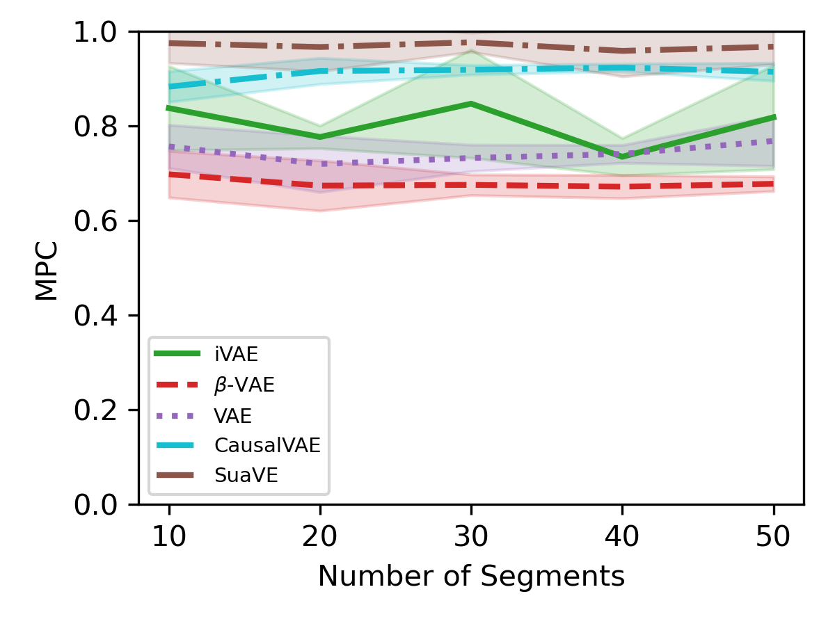
(a)

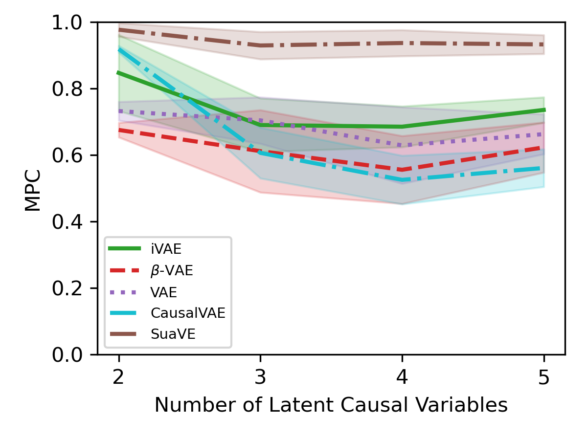
(b)

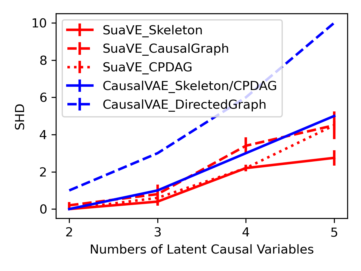
(c)

Figure 5: Performances of the proposed SuaVE in comparison to iVAE, $\beta$-VAE, VAE and CausalVAE in recovering the latent causal variables on synthetic data with different numbers of segments (a), and with different numbers of the latent causal variables (b). The proposed SuaVE obtain the best MPC, compared with the others. (c) The SHD obtained by the proposed SuaVE and CausalVAE.

Results

We compared the performance of the proposed SuaVE to some variants of VAE mentioned above. We used the same network architecture for encoder and decoder parts in all these models. In particular, we add a sub-network to model the conditional prior in both iVAE and the proposed SuaVE. We further assign a linear SCM sub-network to model the relations among latent causal variables in the proposed SuaVE. We trained these 5 models on the dataset described above, with different numbers of segments and different numbers of latent causal variables. For each method, we use 5 different random seeds for data sampling. Figure 5 (a) shows the performance on two latent causal variables with different numbers of segment. The proposed SuaVE obtains the score 0.96 approximately for all the different numbers of segment. In contrast, $\beta$-VAE, VAE and CausalVAE fail to achieve a good estimation of the true latent variables, since they are not identifiable. iVAE obtains unsatisfactory results, since its theory only holds for i.i.d. latent variables. Figure 5 (b) shows the performance in recovering latent causal variables on synthetic data with different numbers of the latent causal variables. Figure 5 (c) depicts the structural Hamming distance (SHD) of the recovered skeletons, causal graphs and completed partial directed acyclic graphs (CPDAG) by the proposed SuaVE and CausalVAE. Since CausalVAE obtains fully connected graphs, the SHD of the recovered CPDAG is the same as one of the recovered skeletons.

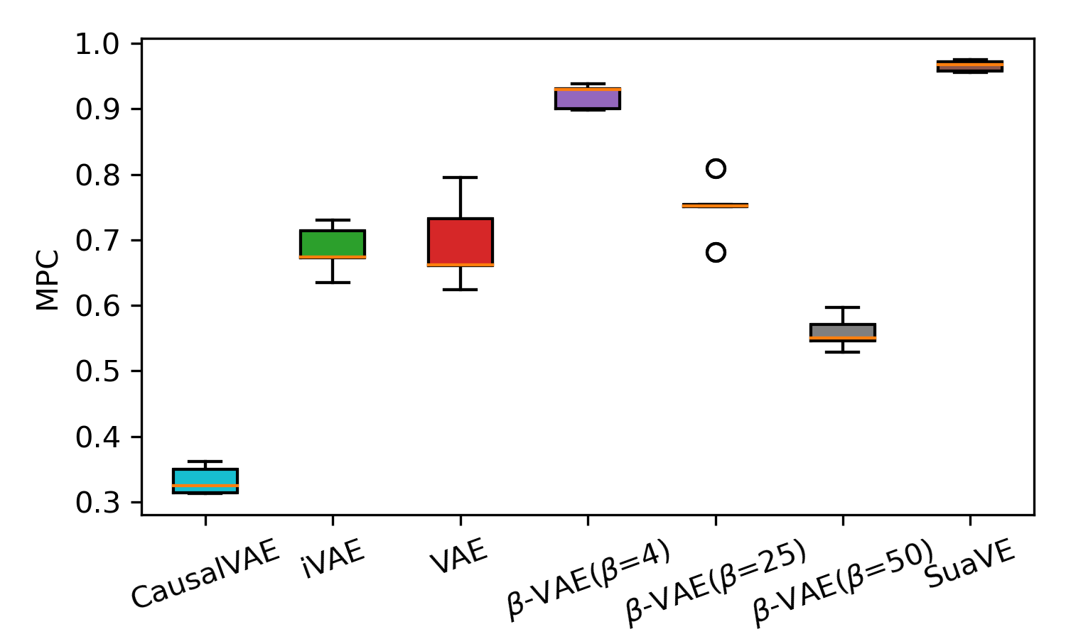
(a)

(b)

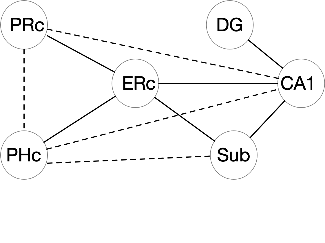
(c)

Figure 6: Performance on fMRI Data. (a) the performance of the proposed SuaVE in comparison to iVAE, $\beta$-VAE, VAE and CausalVAE in recovering the latent six signals. (b) The skeleton of the anatomical connections given in Bird & Burgess (2008). (c) The recovered skeleton by the proposed SuaVE, where the dashed lines indicate errors.

fMRI Data

Following Ghassami et al. (2018), we applied the proposed method to fMRI hippocampus dataset (Laumann & Poldrack, 2015), which contains signals from six separate brain regions: perirhinal cortex (PRC), parahippocampal cortex (PHC), entorhinal cortex (ERC), subiculum (Sub), CA1, and CA3/Dentate Gyrus (DG) in the resting states on the same person in 84 successive days. Each day is considered as different $\mathbf{u}$, thus $\mathbf{u}$ is a 84-dimensional vector. Since we are interested in recovering latent causal variables, we treat the six signals as latent causal variables by applying a random nonlinear mapping on them to obtain observed data. We then apply various methods on the observed data to recover the six signals. Figure 6 (a) shows the performance of the proposed SuaVE in comparison to iVAE, $\beta$-VAE, VAE and CausalVAE in recovering the latent six signals. $\beta$-VAE aims to recover independent latent variables, and it obtains an interesting result: enforcing independence (e.g., $\beta=25,50$) leads to worse MPC, and relaxing it (though contracting to its own independence assumption) improves the result (e.g. $\beta=4$). This is because the latent variables given the time index are not independent in this dataset.

We further verify the ability of the proposed method to recover causal skeleton. We use the anatomical connections (Bird & Burgess, 2008) as a reference as shown in Figure 6 (b), since causal connections among the six regions should not exist if there is no anatomical connection. After recovering the latent causal variables, we estimate the causal skeleton by a threshold (0.1) on the learned $\mathbf{\lambda}_{i,j}$ to remove some edges, and obtain the final causal skeleton. Figure 6 (c) shows an example of the estimated causal skeleton by the proposed SuaVE. Averaging over 5 different random seeds for the used nonlinear mapping from latent space to observed space, structural Hamming distance (SHD) obtained by the proposed SuaVE is 5.0 $\pm$ 0.28. In contrast, iVAE, $\beta$-VAE and VAE assume latent variables to be independent, and thus can not obtain the causal skeleton. We further analyse the result of $\beta$-VAE with $\beta=4$ by using the PC algorithm (Spirtes et al., 2001) to discovery skeleton on the recovered latent variables, and obtain SHD = 5.8 $\pm$ 0.91. This means that: 1) $\beta$-VAE with $\beta=4$ does not ensure the strong independence among the recover latent variables as it is expected, 2) the proposed SuaVE is an effective one-step method to discovery the skeleton. The unsupervised version of CausalVAE is not identifiable, and can also not ensure the relations among the recover variables to be causal skeleton in principle. In experiments we found that CausalVAE always obtains fully-connected graphs for the 5 different random seeds, for which SHD is 9.0 $\pm$ 0.

Table 1: Performance for violated assumptions. Uniform (Laplace, Gamma) Noise: the distribution of latent noise variables. Unchanged Weights: weights keep unchanged across $\mathbf{u}$. Violated assumption (v): $\lambda_{i,j}({\mathbf{0}})=c$ where $c$ a non-zero constant. Matching Assumptions: a setting that matches our theoretical assumptions.

Generative process	MPC(Mean $\pm$ Std)
Uniform Noise	0.83 $\pm$ 0.09
Laplace Noise	0.83 $\pm$ 0.03
Gamma Noise	0.82 $\pm$ 0.05
Unchanged Weights	0.85 $\pm$ 0.09
Violated Assumption (v)	0.87 $\pm$ 0.05
Matching Assumptions	0.95 $\pm$ 0.01

Performance for violated assumptions

To further understand the assumptions of our identifiability result, we conduct experiments in the setting where the assumptions are violated. Table 1 shows the performance for violated assumptions. We can see that violated assumption (v) and unchanged weights obtain similar performance. This is consistent with our analysis of Assumption (v) in section A.2. In addition, the possible reasons for the results of Uniform (Laplace, Gamma) Noise may be: 1) the proposed method enforces Gaussian prior and posterior to approximate non-Gaussian noise, 2) the settings of Uniform (Laplace, Gamma) Noise may be nonidentifiable.

7 Conclusion

Identifying latent causal representations is known to be generally impossible without certain assumptions. Motivated by recent progress in the identifiability result of nonlinear ICA, we analyse three intrinsic indeterminacies in latent space, e.g., transitivity, permutation indeterminacy and scaling indeterminacy, which provide deep insights for identifying latent causal representations. To address the unidentifiable issue due to transitivity, we explore a new line of research in the identifiability of latent causal representations, that of allowing the causal influences among the latent causal variables to change. We show that latent causal representations, modeled by weight-variant linear Gaussian models, can be identified up to permutation and scaling, with mild assumptions. We then propose a novel method to consistently learn latent causal representations. Experiments on synthetic and fMRI data demonstrate the identifiability and consistency results and the efficacy of the proposed method.

Appendix A Appendix

A.1 The proof of Theorem 4.1

The proof of Theorem 4.1 is done in three steps. Step I is to show the identifiability result of nonlinear ICA holds in our setting where there is an additional mapping from $\mathbf{n}$ to $\mathbf{z}$, and the mapping changes across $\mathbf{u}$. Step II consists of building a linear transformation between the true latent variables $\mathbf{z}$ and the estimated ones $\mathbf{\hat{z}}$. Step III shows that the linear transformation in Step II can be reduced to permutation transformation by using the result of Step I and the assumption (v).

Step I: For convenience, let us discuss the property of the mapping from $\mathbf{n}$ to $\mathbf{z}$ first, which plays a key role in the proof. Let function $\mathbf{g}_{\mathbf{u}}$ denote the mapping from $\mathbf{n}$ to $\mathbf{z}$. That is:

$$\mathbf{z}=\mathbf{g}_{\mathbf{u}}(\mathbf{n})=(\mathbf{I}-\boldsymbol{\lambda}^{T}(\mathbf{u}))^{-1}\mathbf{n},$$ (13)

where $\mathbf{I}$ denotes the identity matrix. Due to DAG constraints in a causal system and the assumption of linear models on $\mathbf{z}$, we have 1) the determinant of the Jacobian matrix is equal to 1, e.g., $\det{\mathbf{J}}_{\mathbf{g_{u}}^{-1}}(\mathbf{z})=\det{\mathbf{J}}_{\mathbf{g_{u}}}(\mathbf{u})=1$, 2) the mapping $\mathbf{g}_{\mathbf{n}}$ is invertible.

Suppose we have two sets of parameters $\theta=({\mathbf{f},\mathbf{T}_{\mathbf{n}},\boldsymbol{\lambda},\boldsymbol{\beta}})$ and $\hat{\theta}=({\mathbf{\hat{f}},\mathbf{\hat{T}}_{\mathbf{n}},\boldsymbol{\hat{\lambda}},\boldsymbol{\hat{\beta}}})$ such that $p_{({\mathbf{f},\mathbf{T}_{\mathbf{n}},\boldsymbol{\lambda},\boldsymbol{\beta}})}(\mathbf{x}|\mathbf{u})=p_{({\mathbf{\hat{f}},\mathbf{\hat{T}}_{\mathbf{n}},\boldsymbol{\hat{\lambda}},\boldsymbol{\hat{\beta}}})}(\mathbf{x}|\mathbf{u})$ for all pairs $(\mathbf{x},\mathbf{u})$. Due to the assumption (i), the assumption (ii) that $\mathbf{f}$ is bijective and the fact that $\mathbf{g}_{\mathbf{n}}$ is invertible, by expanding these expressions via the change of variables formula and taking the logarithm we have:

$$\log{|\det\mathbf{J}_{(\mathbf{f}\circ\mathbf{g_{u}})^{-1}}(\mathbf{x})|}+\log p_{\mathbf{(\mathbf{T}_{\mathbf{n}},\boldsymbol{\beta})}}({\mathbf{n}|\mathbf{u}})=\log{|\det\mathbf{J}_{(\mathbf{\hat{f}}\circ\mathbf{\hat{g}_{u}})^{-1}}(\mathbf{x})|}+\log p_{\mathbf{(\mathbf{\hat{T}}_{\mathbf{\hat{n}}},\boldsymbol{\hat{\beta}})}}({\mathbf{\hat{n}}|\mathbf{u}}),$$ (14)

Using the exponential family Eq. (4) to replace $p_{\mathbf{(\mathbf{T}_{\mathbf{n}},\boldsymbol{\beta})}}({\mathbf{n}|\mathbf{u}})$, we have:

$$\log{|\det\mathbf{J}_{(\mathbf{f}\circ\mathbf{g_{u}})^{-1}}(\mathbf{x})|}+\mathbf{T}^{T}_{\mathbf{n}}\big{(}(\mathbf{f}\circ\mathbf{g_{u}})^{-1}(\mathbf{x})\big{)}\boldsymbol{\eta}_{\mathbf{n}}(\mathbf{u})-\log{Z_{\mathbf{n}}(\boldsymbol{\beta},\mathbf{u})}=$$ (15)

$$\log{|\det\mathbf{J}_{(\mathbf{\hat{f}}\circ\mathbf{\hat{g}_{u}})^{-1}}(\mathbf{x})|}+\mathbf{\hat{T}}_{\mathbf{\hat{n}}}^{T}\big{(}(\mathbf{\hat{f}}\circ\mathbf{\hat{g}_{u}})^{-1}(\mathbf{x})\big{)}\boldsymbol{\hat{\eta}}_{\mathbf{n}}(\mathbf{u})-\log{\hat{Z}_{\mathbf{\hat{n}}}(\boldsymbol{\hat{\beta}},\mathbf{u})},$$ (16)

By using:

$$\det\mathbf{J}_{(\mathbf{f}\circ\mathbf{g_{u}})^{-1}}(\mathbf{x})$$ (17)

$$= \det\mathbf{J}_{\mathbf{g}_{\mathbf{u}}^{-1}\circ\mathbf{f}^{-1}}(\mathbf{x})$$

$$= \det\Big{(}\mathbf{J}_{\mathbf{g}_{\mathbf{u}}^{-1}}(\mathbf{f}^{-1}(\mathbf{x}))\mathbf{J}_{\mathbf{f}^{-1}}(\mathbf{x})\Big{)}$$

$$= \det\mathbf{J}_{\mathbf{g}_{\mathbf{u}}^{-1}}(\mathbf{f}^{-1}(\mathbf{x}))\det\mathbf{J}_{\mathbf{f}^{-1}}(\mathbf{x})$$

$$= \det\mathbf{J}_{\mathbf{f}^{-1}}(\mathbf{x}),$$

where the laster derivation is from the fact that $\det{\mathbf{J}}_{\mathbf{g_{u}}^{-1}}(\mathbf{z})=\det{\mathbf{J}}_{\mathbf{g_{u}}}(\mathbf{u})=1$. Obviously, the term $\det\mathbf{J}_{\mathbf{f}^{-1}}(\mathbf{x})$ does not depend on $\mathbf{u}$ as $\mathbf{f}$ is invariant across $\mathbf{u}$. As a result, Eqs. (15)-(16) can be reduced to:

$$\log{|\det\mathbf{J}_{\mathbf{f}^{-1}}(\mathbf{x})|}+\mathbf{T}^{T}_{\mathbf{n}}\big{(}(\mathbf{f}\circ\mathbf{g_{u}})^{-1}(\mathbf{x})\big{)}\boldsymbol{\eta}_{\mathbf{n}}(\mathbf{u})-\log{Z_{\mathbf{n}}(\boldsymbol{\beta},\mathbf{u})}=$$ (18)

$$\log{|\det\mathbf{J}_{\mathbf{\hat{f}}^{-1}}(\mathbf{x})|}+\mathbf{\hat{T}}_{\mathbf{\hat{n}}}^{T}\big{(}(\mathbf{\hat{f}}\circ\mathbf{\hat{g}_{u}})^{-1}(\mathbf{x})\big{)}\boldsymbol{\hat{\eta}}_{\mathbf{n}}(\mathbf{u})-\log{\hat{Z}_{\mathbf{\hat{n}}}(\boldsymbol{\hat{\beta}},\mathbf{u})},$$ (19)

The following proof is similar to the proof of Sorrenson et al. (2020). For completeness, we present a slightly simplified proof. With different points in assumption (iii), we can subtract this expression with $\mathbf{u}_{\mathbf{n},0}$ by the expression with $l_{\mathbf{n}}$, $l_{\mathbf{n}}=1,...,2n$. Since the Jacobian terms do not depend on $\mathbf{u}$, the Jacobian terms will be canceled out:

$$\log\frac{Z_{\mathbf{n}}(\boldsymbol{\beta},\mathbf{u}_{\mathbf{n},0})}{Z_{\mathbf{n}}(\boldsymbol{\beta},\mathbf{u}_{\mathbf{n},l_{\mathbf{n}}})}+\mathbf{T}^{T}_{\mathbf{n}}\big{(}(\mathbf{f}\circ\mathbf{g_{u}})^{-1}(\mathbf{x})\big{)}\big{(}\boldsymbol{\eta}_{\mathbf{n}}(\mathbf{u}_{\mathbf{n},l_{\mathbf{n}}})-\boldsymbol{\eta}_{\mathbf{n}}(\mathbf{u}_{\mathbf{n},0})\big{)}=$$ (20)

$$\log\frac{\hat{Z}_{\mathbf{\hat{n}}}(\boldsymbol{\hat{\beta}},\mathbf{u}_{\mathbf{n},0})}{\hat{Z}_{\mathbf{\hat{n}}}(\boldsymbol{\hat{\beta}},\mathbf{u}_{\mathbf{n},l_{\mathbf{n}}})}+\mathbf{\hat{T}}_{\mathbf{\hat{n}}}^{T}\big{(}(\mathbf{\hat{f}}\circ\mathbf{\hat{g}_{u}})^{-1}(\mathbf{x})\big{)}\big{(}\boldsymbol{\hat{\eta}}_{\mathbf{n}}(\mathbf{u}_{\mathbf{n},l_{\mathbf{n}}})-\boldsymbol{\hat{\eta}}_{\mathbf{n}}(\mathbf{u}_{\mathbf{n},0})\big{)}.$$ (21)

Combining the $2n$ expressions into a single matrix equation we can write it in terms of $\mathbf{L}_{\mathbf{n}}$ from assumption (iii):

$$\mathbf{L}^{T}_{\mathbf{n}}\mathbf{T_{\mathbf{n}}\big{(}(\mathbf{f}\circ\mathbf{g_{u}})^{-1}(x)\big{)}}=\mathbf{\hat{L}}^{T}_{\mathbf{\hat{n}}}\mathbf{\hat{T}_{\mathbf{\hat{n}}}\big{(}(\mathbf{\hat{f}}\circ\mathbf{\hat{g}_{u}})^{-1}(x)\big{)}}+\mathbf{b}_{\mathbf{n}},$$ (22)

where $\mathbf{L}_{\mathbf{n}}$ is defined as the assumption (iii), $\mathbf{b}_{\mathbf{n},l_{\mathbf{n}}}=\log\frac{\hat{Z}_{\mathbf{\hat{n}}}(\boldsymbol{\hat{\beta}},\mathbf{u}_{\mathbf{n},0})Z_{\mathbf{n}}(\boldsymbol{\beta},\mathbf{u}_{\mathbf{n},l_{\mathbf{n}}})}{\hat{Z}_{\mathbf{\hat{n}}}(\boldsymbol{\hat{\beta}},\mathbf{u}_{\mathbf{n},l_{\mathbf{n}}})Z_{\mathbf{n}}(\boldsymbol{\beta},\mathbf{u}_{\mathbf{n},0})}$. Since $\mathbf{L}^{T}_{\mathbf{n}}$ is invertible by the assumption (iii), we can multiply this expression by its inverse:

$$\mathbf{T_{\mathbf{n}}\big{(}(\mathbf{f}\circ\mathbf{g_{u}})^{-1}(x)\big{)}}=\mathbf{A}_{\mathbf{n}}\mathbf{\hat{T}_{\mathbf{\hat{n}}}\big{(}(\mathbf{\hat{f}}\circ\mathbf{\hat{g}_{u}})^{-1}(x)\big{)}}+\mathbf{c}_{\mathbf{n}},$$ (23)

Following Khemakhem et al. (2020); Sorrenson et al. (2020), it is easily to show that $\mathbf{A}_{\mathbf{n}}$ is invertible. Since we assume the noise to be Gaussian, Eq. (23) can be re-expressed as:

$$\left(\begin{array}[]{c}\mathbf{n}\\ \mathbf{n}^{2}\\ \end{array}\right)=\mathbf{A}_{\mathbf{n}}\left(\begin{array}[]{c}\mathbf{\hat{n}}\\ \mathbf{\hat{n}}^{2}\\ \end{array}\right)+\mathbf{c}_{\mathbf{n}},$$ (24)

Then, by the contradiction between 1) for every $n_{i}$, there exists a polynomial with a degree at most 2, and 2) for every $n^{2}_{i}$, there also exists a polynomial with a degree at most 2 (Sorrenson et al., 2020), we can obtain:

$$\mathbf{n}=\mathbf{P}\mathbf{\hat{n}}+\mathbf{c}_{\mathbf{n}},$$ (25)

where $\mathbf{P}$ denote the permutation matrix with scaling.

Step II: Again, suppose we have two sets of parameters $\theta=({\mathbf{f},\mathbf{T}_{\mathbf{z}},\boldsymbol{\lambda},\boldsymbol{\beta}})$ and $\hat{\theta}=({\mathbf{\hat{f}},\mathbf{\hat{T}}_{\mathbf{z}},\boldsymbol{\hat{\lambda}},\boldsymbol{\hat{\beta}}})$ such that $p_{({\mathbf{f},\mathbf{T}_{\mathbf{z}},\boldsymbol{\lambda},\boldsymbol{\beta}})}(\mathbf{x}|\mathbf{u})=p_{({\mathbf{\hat{f}},\mathbf{\hat{T}}_{\mathbf{z}},\boldsymbol{\hat{\lambda}},\boldsymbol{\hat{\beta}}})}(\mathbf{x}|\mathbf{u})$ for all pairs $(\mathbf{x},\mathbf{u})$. Due to the assumptions (i) and (ii), by expanding these expressions via the change of variables formula and taking the logarithm we have:

$$\log{|\det\mathbf{J}_{\mathbf{f}^{-1}}(\mathbf{x})|}+\log p_{\mathbf{(\mathbf{T}_{\mathbf{z}},\boldsymbol{\lambda},\boldsymbol{\beta})}}({\mathbf{z}|\mathbf{u}})=\log{|\det\mathbf{J}_{\mathbf{\hat{f}}^{-1}}(\mathbf{x})|}+\log p_{\mathbf{(\mathbf{\hat{T}}_{\mathbf{\hat{z}}},\boldsymbol{\hat{\lambda}},\boldsymbol{\hat{\beta}})}}({\mathbf{\hat{z}}|\mathbf{u}}),$$ (26)

Using the exponential family Eq. (7) to replace $p_{\mathbf{(\mathbf{T}_{\mathbf{z}},\boldsymbol{\lambda},\boldsymbol{\beta})}}({\mathbf{z}|\mathbf{u}})$:

$$\log{|\det\mathbf{J}_{\mathbf{f}^{-1}}(\mathbf{x})|}+\mathbf{T}^{T}_{\mathbf{z}}(\mathbf{f}^{-1}(\mathbf{x}))\boldsymbol{\eta}_{\mathbf{z}}(\mathbf{u})-\log{Z_{\mathbf{z}}(\boldsymbol{\lambda},\boldsymbol{\beta},\mathbf{u})}=$$ (27)

$$\log{|\det\mathbf{J}_{\mathbf{\hat{f}}^{-1}}(\mathbf{x})|}+\mathbf{\hat{T}}^{T}_{\mathbf{\hat{z}}}(\mathbf{\hat{f}}^{-1}(\mathbf{x}))\boldsymbol{\hat{\eta}}_{\mathbf{\hat{z}}}(\mathbf{u})-\log{\hat{Z}_{\mathbf{\hat{z}}}(\boldsymbol{\hat{\lambda}},\boldsymbol{\hat{\beta}},\mathbf{u})}.$$ (28)

Let $\mathbf{u}_{\mathbf{z},0},\mathbf{u}_{\mathbf{z},1},...,\mathbf{u}_{\mathbf{z},k}$ be the points provided by the assumption (iv). We define $\bar{\boldsymbol{\eta}}_{\mathbf{z}}(\mathbf{u}_{\mathbf{z},l_{\mathbf{z}}})={\boldsymbol{\eta}}_{\mathbf{z}}(\mathbf{u}_{\mathbf{z},l_{\mathbf{z}}})-{\boldsymbol{\eta}_{\mathbf{z}}}(\mathbf{u}_{\mathbf{z},0})$. We plug each of those $\mathbf{u}_{\mathbf{z},l_{\mathbf{z}}},l_{\mathbf{z}}=1,...,k$ in Eq. (28) to obtain $k+1$ equations. We subtract the first equation for $\mathbf{u}_{\mathbf{z},0}$ from the remaining $k$ equations. For example, for $\mathbf{u}_{\mathbf{z},0}$ and $\mathbf{u}_{\mathbf{z},l_{\mathbf{z}}}$ we have two equations:

$$\log{|\det\mathbf{J}_{\mathbf{f}^{-1}}(\mathbf{x})|}+\mathbf{T}^{T}_{\mathbf{z}}(\mathbf{f}^{-1}(\mathbf{x}))\boldsymbol{\eta}_{\mathbf{z}}(\mathbf{u}_{\mathbf{z},0})-\log{Z_{\mathbf{z}}(\boldsymbol{\lambda},\boldsymbol{\beta},\mathbf{u}_{\mathbf{z},0})}=$$ (29a)

$$\log{|\det\mathbf{J}_{\mathbf{\hat{f}}^{-1}}(\mathbf{x})|}+\mathbf{\hat{T}}^{T}_{\mathbf{z}}(\mathbf{\hat{f}}^{-1}(\mathbf{x}))\boldsymbol{\hat{\eta}}_{\mathbf{\hat{z}}}(\mathbf{u}_{\mathbf{z},0})-\log{\hat{Z}_{\mathbf{\hat{z}}}(\boldsymbol{\hat{\lambda}},\boldsymbol{\hat{\beta}},\mathbf{u}_{\mathbf{z},0})},$$

$$\log{|\det\mathbf{J}_{\mathbf{f}^{-1}}(\mathbf{x})|}+\mathbf{T}^{T}_{\mathbf{z}}(\mathbf{f}^{-1}(\mathbf{x}))\boldsymbol{\eta}_{\mathbf{z}}(\mathbf{u}_{\mathbf{z},l_{\mathbf{z}}})-\log{Z_{\mathbf{z}}(\boldsymbol{\lambda},\boldsymbol{\beta},\mathbf{u}_{\mathbf{z},l_{\mathbf{z}}})}=$$ (29b)

$$\log{|\det\mathbf{J}_{\mathbf{\hat{f}}^{-1}}(\mathbf{x})|}+\mathbf{\hat{T}}^{T}_{\mathbf{z}}(\mathbf{\hat{f}}^{-1}(\mathbf{x}))\boldsymbol{\hat{\eta}}_{\mathbf{\hat{z}}}(\mathbf{u}_{\mathbf{z},l_{\mathbf{z}}})-\log{\hat{Z}_{\mathbf{\hat{z}}}(\boldsymbol{\hat{\lambda}},\boldsymbol{\hat{\beta}},\mathbf{u}_{\mathbf{z},l_{\mathbf{z}}})},$$

Using Eq. (29b) subtracts Eq. (29a), canceling the terms that do not include $\mathbf{u}$, we have:

$$\log\frac{Z_{\mathbf{z}}(\boldsymbol{\lambda},\boldsymbol{\beta},\mathbf{u}_{\mathbf{z},0})}{Z_{\mathbf{z}}(\boldsymbol{\lambda},\boldsymbol{\beta},\mathbf{u}_{\mathbf{z},l_{\mathbf{z}}})}+\mathbf{T}_{\mathbf{z}}{(\mathbf{f}^{-1}(\mathbf{x}))}\big{(}\boldsymbol{\eta}_{\mathbf{z}}(\mathbf{u}_{\mathbf{z},l_{\mathbf{n}}})-\boldsymbol{\eta}_{\mathbf{z}}(\mathbf{u}_{\mathbf{z},0})\big{)}=\log\frac{\hat{Z}_{\mathbf{\hat{z}}}(\boldsymbol{\hat{\lambda}},\boldsymbol{\hat{\beta}},\mathbf{u}_{\mathbf{z},0})}{\hat{Z}_{\mathbf{\hat{z}}}(\boldsymbol{\hat{\lambda}},\boldsymbol{\hat{\beta}},\mathbf{u}_{\mathbf{z},l_{\mathbf{z}}})}+\mathbf{\hat{T}}_{\mathbf{\hat{z}}}{(\mathbf{\hat{f}}^{-1}(\mathbf{x}))}\big{(}\boldsymbol{\hat{\eta}}_{\mathbf{\hat{z}}}(\mathbf{u}_{\mathbf{z},l_{\mathbf{n}}})-\boldsymbol{\hat{\eta}}_{\mathbf{\hat{z}}}(\mathbf{u}_{\mathbf{z},0})\big{)}.$$ (30)

Let $\mathbf{L}_{\mathbf{z}}$ be the matrix defined in Eq. (9) in assumption (iv), and $\mathbf{\hat{L}}_{\mathbf{\hat{z}}}$ similarly ($\mathbf{\hat{L}}_{\mathbf{\hat{z}}}$ is not necessarily invertible). Define $b_{\mathbf{z},l_{\mathbf{z}}}={\log{\frac{\hat{Z}_{\mathbf{\hat{z}}}(\boldsymbol{\hat{\lambda}},\boldsymbol{\hat{\beta}},\mathbf{u}_{\mathbf{z},0})Z_{\mathbf{z}}(\boldsymbol{\lambda},\boldsymbol{\beta},\mathbf{u}_{\mathbf{z},l_{\mathbf{z}}})}{Z_{\mathbf{z}}(\boldsymbol{\lambda},\boldsymbol{\beta},\mathbf{u}_{\mathbf{z},0})\hat{Z}_{\mathbf{\hat{z}}}(\boldsymbol{\hat{\lambda}},\boldsymbol{\hat{\beta}},\mathbf{u}_{\mathbf{z},l_{\mathbf{z}}})}}}$. Expressing Eq. (30) for all points in matrix form, we get:

$$\mathbf{L}_{\mathbf{z}}^{T}\mathbf{T_{\mathbf{z}}(f^{-1}(x))}=\mathbf{\hat{L}}_{\mathbf{\hat{z}}}^{T}\mathbf{\hat{T}_{\mathbf{z}}(\hat{f}^{-1}(x))}+\mathbf{b}_{\mathbf{z}}.$$ (31)

We multiply both sides of Eq. (31) by the inverse of $\mathbf{L}^{T}_{\mathbf{z}}$ (by assumption (iv)) to find:

$$\mathbf{T_{\mathbf{z}}(f^{-1}(x))}=\mathbf{A}_{\mathbf{z}}\mathbf{\hat{T}_{\mathbf{\hat{z}}}(\hat{f}^{-1}(x))}+\mathbf{c}_{\mathbf{z}},$$ (32)

where $\mathbf{A}_{\mathbf{z}}=(\mathbf{L}_{\mathbf{z}}^{T})^{-1}\mathbf{\hat{L}}_{\mathbf{\hat{z}}}^{T}$ and $\mathbf{c}_{\mathbf{z}}=(\mathbf{L}_{\mathbf{z}}^{T})^{-1}\mathbf{b}_{\mathbf{z}}$. As mentioned in Eq. (7), the sufficient statistic $\mathbf{T}_{\mathbf{z}}(\mathbf{z})=[\mathbf{z};\operatorname{vec}(\mathbf{z}\mathbf{z}^{T})]$. In this case, the relationship Eq. (32) becomes:

$$\left(\begin{array}[]{c}\mathbf{z}\\ \mathbf{z}^{2}\\ \mathbf{z}_{i\neq j}\\ \end{array}\right)=\mathbf{A}_{\mathbf{z}}\left(\begin{array}[]{c}\mathbf{\hat{z}}\\ \mathbf{\hat{z}}^{2}\\ \mathbf{\hat{z}}_{i\neq j}\\ \end{array}\right)+\mathbf{c}_{\mathbf{z}},$$ (33)

where $\mathbf{z}$ denotes $[z_{1},...,z_{i}]$, $\mathbf{z}^{2}$ denotes $[z^{2}_{1},...,z^{2}_{i}]$, $\mathbf{z}_{i\neq j}$ denotes the vector whose elements are ${z}_{i}{z}_{j}$ for all $i\neq j$, $\mathbf{A}_{\mathbf{z}}$ in block matrix can be rewritten as:

$$\mathbf{A}_{\mathbf{z}}=\left(\begin{array}[]{ccc}\mathbf{A}^{(1)}&\mathbf{A}^{(2)}&\mathbf{A}^{(3)}\\ \mathbf{A}^{(4)}&\mathbf{A}^{(5)}&\mathbf{A}^{(6)}\\ \mathbf{A}^{(7)}&\mathbf{A}^{(8)}&\mathbf{A}^{(9)}\\ \end{array}\right)$$ (34)

and $\mathbf{c}_{\mathbf{z}}$ as:

$$\mathbf{c}_{\mathbf{z}}=\left(\begin{array}[]{c}\mathbf{c}^{(1)}\\ \mathbf{c}^{(2)}\\ \mathbf{c}^{(3)}\\ \end{array}\right).$$ (35)

Then, we have:

$$\mathbf{z}=\mathbf{A}^{(1)}\mathbf{\hat{z}}+\mathbf{A}^{(2)}\mathbf{\hat{z}}^{2}+\mathbf{A}^{(3)}\mathbf{\hat{z}}_{i\neq j}+\mathbf{c}^{(1)},$$ (36)

$$\mathbf{z}^{2}=\mathbf{A}^{(4)}\mathbf{\hat{z}}+\mathbf{A}^{(5)}\mathbf{\hat{z}}^{2}+\mathbf{A}^{(6)}\mathbf{\hat{z}}_{i\neq j}+\mathbf{c}^{(2)}.$$ (37)

So we can write for each ${z}_{i}$:

$${z_{i}}=\sum_{j}({A}_{i,j}^{(1)}{\hat{z}}_{j})+\sum_{j}({A}_{i,j}^{(2)}{\hat{z}^{2}}_{j})+({\mathbf{A}}_{i,:}^{(3)}\hat{\mathbf{z}}_{i\neq j})+{c}_{i}^{(1)},$$ (38)

$$z_{i}^{2}=\sum_{j}({A}_{i,j}^{(4)}{\hat{z}}_{j})+\sum_{j}({A}_{i,j}^{(5)}{\hat{z}^{2}}_{j})+({\mathbf{A}}_{i,:}^{(6)}\hat{\mathbf{z}}_{i\neq j})+{c}_{i}^{(2)}.$$ (39)

Squaring Eq. (38), we have:

$${z}_{i}^{2}= \underbrace{(\sum_{j}({A}_{i,j}^{(2)}{\hat{z}^{2}}_{j}))^{2}}_{\mathbf{(a)}}+\underbrace{(\sum_{j}({A}_{i,j}^{(1)}{\hat{z}}_{j}))^{2}}_{\text{(b)}}+\underbrace{({\mathbf{A}}_{i,:}^{(3)}\hat{\mathbf{z}}_{i\neq j})^{2}}_{\text{(c)}}+({c}_{i}^{(1)})^{2}+.....$$ (40)

It is notable that Eq. (39) and Eq. (40) are derived from Eq. (32) which holds for arbitrary $\mathbf{x}$, then by the assumption (ii) in Theorem 4.1 that $\mathbf{f}$ is a bijective mapping from $\mathbf{z}$ to $\mathbf{x}$, and thus Eq. (39) and Eq. (40) must holds for $\mathbf{z}$ everywhere. Then by the fact that the right sides of the Eq. (39) and Eq. (40) are both polynomials with finite degree, we have each coefficients of the two polynomials must be equal. In more detail, for the term (a) in Eq. (40):

$${(\sum_{j}({A}_{i,j}^{(2)}{\hat{z}^{2}}_{j}))^{2}}=\sum_{j}({A}_{i,j}^{(2)})^{2}{\hat{z}^{4}}_{j}+\sum_{j\neq j^{\prime}}(2{A}_{i,j}^{(2)}{A}_{i,j^{\prime}}^{(2)}{\hat{z}^{2}}_{j}{\hat{z}^{2}}_{j^{\prime}}).$$ (41)

Compared with Eq. (39), since there is no term ${\hat{z}^{4}}_{j}$ in Eq. (39), we must have that:

$$\mathbf{A}^{(2)}=0.$$ (42)

For the term (c) in Eq. (40):

$${({\mathbf{A}}_{i,:}^{(3)}\hat{\mathbf{z}}_{i\neq j})^{2}}={\sum_{j^{{}^{\prime}},i\neq j}({A}_{i,j^{\prime}}^{(3)})^{2}(\hat{z}_{i}\hat{z}_{j})^{2}}+...$$ (43)

Compared with Eq. (39), since there is no term $(\hat{z}_{i}\hat{z}_{j})^{2}$ in Eq. (39), we must have that:

$$\mathbf{A}^{(3)}=0$$ (44)

As a result, Eq. (36) becomes:

$$\mathbf{z}=\mathbf{A}^{(1)}\mathbf{\hat{z}}+\mathbf{c}^{(1)}.$$ (45)

The above equation indicates the latent causal variables can be recovered up to linear transformation.

Step III We then show that the linear transformation matrix $\mathbf{A}^{(1)}$ in Eq. (45) must be a permutation matrix. As we mentioned in step I, for the Gaussian noise variables $\mathbf{n}$, we have:

$$\mathbf{n}=\mathbf{P}\mathbf{\hat{n}}+\mathbf{c}_{n},$$ (46)

where $\mathbf{P}$ denote the permutation matrix with scaling. With Eq. (46), the Eq. (45) can be rewritten as follows:

$$\mathbf{B}(\mathbf{P}\mathbf{\hat{n}}+\mathbf{c}_{n})=\mathbf{A}^{(1)}(\mathbf{\hat{B}}\mathbf{\hat{n}})+\mathbf{c}^{(1)}.$$ (47)

$$\Rightarrow (\mathbf{B}\mathbf{P}-\mathbf{A}^{(1)}\mathbf{\hat{B}})\mathbf{\hat{n}}=\mathbf{c}^{(1)}-\mathbf{B}\mathbf{c}_{n},$$ (48)

where, without loss of generality, $\mathbf{B}$ and $\mathbf{\hat{B}}$ denote a lower triangular matrix, for which the main diagonal are 1, the others depend on $\lambda_{i,j}(\mathbf{u})$ and ${\hat{\lambda}_{i,j}}(\mathbf{u})$, respectively. By differentiating Eq. (48) with respect to $\mathbf{\hat{n}}$, we have:

$$(\mathbf{B}\mathbf{P}-\mathbf{A}^{(1)}\mathbf{\hat{B}})\mathbf{I}=\mathbf{0},$$ (49)

where $\mathbf{I}$ denote the identity matrix, which implies that:

$$\mathbf{B}\mathbf{P}=\mathbf{A}^{(1)}\mathbf{\hat{B}}.$$ (50)

Elements above the diagonal

Since $\mathbf{A}^{(1)}=\mathbf{B}\mathbf{P}\mathbf{\hat{B}}^{-1}$, and both $\mathbf{B}$ and $\mathbf{\hat{B}}$ are lower triangular matrices with diagonal elements 1, and $\mathbf{P}$ is a permutation matrix with scaling, $\mathbf{A}^{(1)}$ must be a lower triangular matrix. That is, elements above the diagonal are equal to 0.

The diagonal elements

Without loss of generality, we assume $\mathbf{P}$ to be diagonal with elements $s_{1,1},s_{2,2},s_{3,3},...$. By expanding the left side of Eq. (50), we have:

$$\mathbf{B}\mathbf{P}=\left(\begin{array}[]{cccc}s_{1,1}&0&0&...\\ s_{1,1}\lambda_{2,1}(\mathbf{u})&s_{2,2}&0&...\\ s_{1,1}\lambda_{3,1}(\mathbf{u})&s_{2,2}\lambda_{3,2}(\mathbf{u})&s_{3,3}&...\\ .&.&.&...\\ \end{array}\right).$$ (51)

Since $\mathbf{\hat{B}}$ in the right side of Eq. (50) is a lower triangular matrix with diagonal elements 1, the diagonal elements of $\mathbf{A}^{(1)}$ must be $s_{1,1},s_{2,2},s_{3,3},...$.

Elements below the diagonal

For each element $\mathbf{A}^{(1)}_{i,j}$ where $i>j$, since the diagonal elements of $\mathbf{\hat{B}}$ are 1, by multiplying the $i$th row of $\mathbf{A}^{(1)}$ and the $j$th column of $\mathbf{\hat{B}}$, we can always obtain: $(\mathbf{A}^{(1)}\mathbf{\hat{B}})_{i,j}=\mathbf{A}^{(1)}_{i,j}+\sum_{j^{\prime}>j}{\mathbf{A}^{(1)}_{i,j^{\prime}}{\hat{\lambda}_{j^{\prime},j}}(\mathbf{u})}$. Then by the fact that $(\mathbf{A}^{(1)}\mathbf{\hat{B}})_{i,j}=(\mathbf{B}\mathbf{P})_{i,j}$, we have: $\mathbf{A}^{(1)}_{i,j}+\sum_{j^{\prime}>j}{\mathbf{A}^{(1)}_{i,j^{\prime}}{\hat{\lambda}_{j^{\prime},j}}(\mathbf{u})}=s_{j,j}\lambda_{i,j}(\mathbf{u})$. Then by assumption (v), we have $\mathbf{A}^{(1)}_{i,j}=0$.

As a result, the matrix $\mathbf{A}^{(1)}$ is the same as the matrix $\mathbf{P}$. That is,

$$\mathbf{z}=\mathbf{P}\mathbf{\hat{z}}+\mathbf{c}_{\mathbf{z}}.$$ (52)

A.2 Understanding Assumptions in Theorem 4.1

Assumptions (i)-(iii)

All three assumptions are motivated by the nonlinear ICA literature (Khemakhem et al., 2020), which is to provide a guarantee that we can recover latent noise variables $\mathbf{n}$ up to a permutation and scaling transformation. Note that assumptions (i)-(ii) also provide support for recovering the latent causal variables up to a linear transformation.

Assumptions (iv)

Similar to nonlinear ICA (Khemakhem et al., 2020), the intuition of assumption (iv) is to enable the weights to vary sufficiently across $\mathbf{u}$, so that there exists a linear relation between the true latent variables $\mathbf{z}$ and the estimated latent variables $\mathbf{\hat{z}}$. Note that the distinct points in $\{\mathbf{u}_{\mathbf{n},0},\mathbf{u}_{\mathbf{n},1},...,\mathbf{u}_{\mathbf{n},2n}\}$ could be overlapping with the distinct points in $\{\mathbf{u}_{\mathbf{z},0},\mathbf{u}_{\mathbf{z},1},...,\mathbf{u}_{\mathbf{z},k}\}$. That is, ideally, we may only need $k$ distinct points, for which both $\mathbf{L}_{\mathbf{n}}$ and $\mathbf{L}_{\mathbf{z}}$ are invertible.

Assumption (v)

Assumption (v) is to avoid a special case as follows: $\lambda_{i,j}({\mathbf{u}})=\lambda^{\prime}_{i,j}{\mathbf{u}}+b$ where $b$ is a non-zero constant. For example, if $z_{2}=(\lambda^{\prime}_{1,2}(\mathbf{u})+b)z_{1}+n_{2}$, then the term $bz_{1}$ is still unchanged across all $\mathbf{u}$, and thus can still be ‘absorbed’ by the nonlinear mapping from latent variables $\mathbf{z}$ to the observed variable $\mathbf{x}$ due to the transitivity, which results in non-identifiability. Assumption (v) is sufficient to handle the special case, but it may not be necessary. Note that assumption (v) is only to restrict the function class for $\lambda_{i,j}({\mathbf{u}})$. That is, it does not require that the observed data include the data corresponding to ${\mathbf{u}}=\mathbf{0}$. There may exist a possible assumption to relax the assumption (v). We expect that a sufficient and necessary condition is proposed in the future to handle the special case above.

Gaussian assumption on the latent noise variables

Our first assumption is implicitly enforcing Gaussian distribution on the latent noise variables. Note that the assumptions of nonlinear ICA (Khemakhem et al., 2020) on the noise could be broad exponential family distribution, e.g., Gaussian distributions, Laplace, Gamma distribution, and so on. This work considers Gaussian distribution, mainly because it can be straightforwardly implemented for the re-parameterization trick in VAE. 2) it is convenient for simplifying the proof process. It is worthwhile and promising to extend the Gaussian assumption to exponential family for future work.

Linear model assumption for the latent causal variables

As the first work to discuss the relation between the change of causal influences and identifiability of latent causal model, this work simply considers linear models for the latent causal variables, because it can be directly parameterized, which helps us to analyze the challenge of identifiability and how to handle it. In addition, together with Gaussian noise, we arrive at the same probabilistic model as linear Gaussian Bayesian networks, which is a well-studied model as mentioned in Eq. (6). We expect that the proposed weights-variant linear models can motivate more general functional classes in future work, e.g., nonlinear additive noise models.

Changes of weights

We allow changes of weight (e.g., causal influences) among latent causal variables across $\mathbf{u}$ to handle the transitivity problem. We argue that this is not a necessary condition for identifiability (Existing methods, including sparse graph structure and temporal information, could be regarded as feasible ways to handle the transitivity.), but it is a sufficient condition to handle the transitivity, and provide a new research line for causal representation learning. In fact, exploring the change of causal influences is not new in observed space (Ghassami et al., 2018; Huang* et al., 2020). In addition, identifying latent causal representation by randomly chosen unknown hard intervention Brehmer et al. (2022) can also be regarded as a special change of causal influences. For this viewpoint, we argue that exploring the change of causal influences for identifying latent causal representation is a promising way and not too restricted in reality.

We emphasize that we require the change of weights among latent causal variables across $\mathbf{u}$. But this does not imply that the weights always change across $\mathbf{u}$. That is, some weights are allowed to keep unchanged for some points $\mathbf{u}$, as long as these weights change for other points $\mathbf{u}^{\prime}$. See experimental results in section A.7 for further discussion.

A.3 The Proof of Corollary 4.2

Theorem 4.1 has shown that the latent causal variables $\mathbf{z}$ can be identified up to trivial permutation and linear scaling. Hence, the identifiability of the causal structure in latent space can be reduced to the identifiability of the causal structure in observed space. Moreover, we need to show that the linear scaling does not affect theoretical identifiability of the causal structure.

For the identifiability of the causal structure in observed space from heterogeneous data, fortunately, we can leverage the results from Huang* et al. (2020). Corollary 4.2 relies on the Markov condition and faithfulness assumption and the assumption that the latent change factor (i.e., causal strength in the linear case) can be represented as a function of the domain index $\mathbf{u}$. Hence, it relies on the same assumptions as that in Huang* et al. (2020).

It has been shown in Huang* et al. (2020) that if the joint distribution over $\mathbf{z}$ and $\mathbf{u}$ ($\mathbf{z}$ and $\mathbf{u}$ are observed variables here) are Markov and faithful to the augmented graph, then the causal structure over $\mathbf{z}\cup\mathbf{u}$ can be identified up to the Markov equivalence class, by making use of the conditional independence relationships.

Next, we show that the Markov equivalence class over $\mathbf{z}$ is also identifiable. Denote by $M$ the Markov equivalence class over $\mathbf{z}\cup\mathbf{u}$, and by $M_{z}$ the Markov equivalence class over $\mathbf{z}$. Then after removing variable $\mathbf{u}$ in $M$ and its edges, the resulting graph (denoted by $M’_{z}$) is the same as $M_{z}$. This is because of the following reasons. First, it is obvious that $M’_{z}$ and $M_{z}$ have the same skeleton. Second, in this paper, $\mathbf{u}$ has an edge to every $z_{i}$ when considering $\mathbf{n}$ as latent noise variables, because all causal strength and noise distributions change with $\mathbf{u}$. Hence, there is no v-structure over $\mathbf{u}$, $z_{i}$, and $z_{j}$, so it is not possible to have more oriented edges in $M’_{z}$. Therefore, $M’_{z}$ and $M_{z}$ have the same skeleton and the same directions.

Moreover, the conditional independence relationships will not be affected by linear scaling of the variables, so the conditional independence relationships still hold in the identified latent variables. Furthermore, for linear-Gaussian models, independence equivalence is the same as distributional equivalence. This is because of the following reasons. First, since we are concerned with linear Gaussian models over the latent variables, the identifiability up to equivalence class also holds for score-based methods that use the likelihood of data as objective functions. This is because independence equivalence, i.e., two DAGs have the same conditional independence relations, is the same as distributional equivalence for linear-Gaussian models, i.e., two Bayesian networks corresponding to the two DAGs can define the same probability distribution. That is to say, score-based methods also find the structure based on independence relations implicitly. Because the scaling does not change the independence relations, it will also not affect the identifiability of the graph structure.

Therefore, the causal structure among latent variables $\mathbf{z}$ can be identified up to the Markov equivalence class.

A.4 The Proof of Corollary 4.3

To prove this corollary, let us introduce ICM first.

Definition A.1.

(Independent Causal Mechanisms). In a causally sufficient system, the causal modules, as well as their included parameters, change independently across domains.

Here we follow Ghassami et al. (2018) to define ICM principle. Another slightly different definition appears in Peters et al. (2017); Schölkopf et al. (2021). Both two definitions imply the same principle that the causal modules change independently across $\mathbf{u}$. According to ICM principle, in the causal direction, the causal modules, as well as their included parameters, change independently across $\mathbf{u}$. However, such independence generally does not hold in the anti-causal direction (Ghassami et al., 2018; Huang* et al., 2020). For example, consider $z_{1}$ and $z_{2}$ in Figure 1. According to model definition in Eq. (1)- Eq. (3), for causal direction $z_{1}\rightarrow z_{2}$, we have:

$$z_{1}:=n_{1},\qquad z_{2}:=\lambda_{1,2}({\mathbf{u}})z_{1}+n_{2}.$$ (53)

For the reverse direction, we have

$$\begin{split}&z_{1}=\lambda^{\prime}_{1}(\mathbf{u})z_{2}+n_{1}^{\prime},\qquad\qquad\qquad\qquad\ z_{2}=n_{2}^{\prime}\\ &\lambda^{\prime}_{1}(\mathbf{u})=\frac{1}{\lambda_{1,2}(\mathbf{u})},\quad n_{1}^{\prime}=-\frac{1}{\lambda_{1,2}(\mathbf{u})}n_{2}\qquad n_{2}^{\prime}=\lambda_{1,2}({\mathbf{u}})z_{1}+n_{2}\end{split}$$ (54)

In this case, the module $p(z_{2})$ is dependent of the module $p(z_{1}|z_{2})$, e.g., both modules depend on the same parameter $\lambda_{1,2}({\mathbf{u}})$, which violates ICM principle. Clearly, the scaling indeterminacy for the recovered latent variables does not affect such dependence. As a result, regardless of the scaling, with the help of ICM, we can fully identify the acyclic causal structure among latent variables $\mathbf{z}$.

A.5 The proof of Theorem 5.1

The proof of Theorem 5.1 is similar to the proof of Theorem 4 in non-linear ICA (Khemakhem et al., 2020). If the variational posterior $q(\mathbf{z}|\mathbf{x,u})$ is large enough to include the true posterior $p(\mathbf{z}|\mathbf{x,u})$, then by optimizing the loss, the KL term will be zero, and the loss will be equal to the log-likelihood. Since our identifiability is guaranteed up to permutation and scaling, the consistency of maximum log-likelihood means that we converge to the true latent causal variables up to permutation and scaling classes, in the limit of infinite data.

A.6 Implementation Details

A.6.1 Experiments for Figure 5 (a)

Data

For experimental results of Figure 5 (a) the number of segments (e.g.,$\mathbf{u}$) $M$ is 10,20,30,40 and 50 respectively. For each segment, the number of latent causal variables is 2 and the sample size is 1000. We consider the following structural causal model

$$n_{1}:={\cal N}({\beta}(\mathbf{u})_{1,1},{\beta}(\mathbf{u})_{1,2}),\qquad n_{2}:={\cal N}({\beta}(\mathbf{u})_{2,1},{\beta}(\mathbf{u})_{2,2}),$$ (55)

$${z_{1}}:=n_{1},\qquad\qquad\qquad\qquad\quad\ \ {z_{2}}:=\lambda_{1,2}(\mathbf{u}){z_{1}}+n_{2},$$ (56)

where we sample the mean ${\beta}(\mathbf{u})_{i,1}$ and variance ${\beta}(\mathbf{u})_{i,2}$ from uniform distributions $[-2,2]$ and $[0.01,3]$, respectively. We sample the weights $\lambda_{1,2}(\mathbf{u})$ from uniform distributions $[0.1,2]$. We sample latent variable z according to Eqs. 55 and 56, and then mix them using a 2-layer multi-layer perceptron (MLP) to generate observed $\mathbf{x}$.

Network and Optimization

For all methods, we used a encoder, e.g. 3-layer fully connected network with 30 hidden nodes and Leaky-ReLU activation functions, and decoder, e.g. 3-layer fully connected network with 30 hidden nodes and Leaky-ReLU activation functions. We also use 3-layer fully connected network with 30 hidden nodes and Leaky-ReLU activation functions. For optimization, we use Adam optimizer with learning rate $1r=1e-3$. For hyper-parameters, we set $\beta=4$ for the $\beta$-VAE. For CausalVAE, we set the hyper-parameters as suggested in the paper (Yang et al., 2021).

A.6.2 Experiments for Figure 5 (b) and (c)

Data

For experimental results of Figure 5 (b) and (c), the number of segments is $30$ and sample size is 1000, while the number (e.g., dimension) of latent causal variables is 2,3,4,5 respectively. For 2-dimensional latent causal variables, the setting is the same as experiments for Figure 5 (a). For 3-dimensional case, we consider the following structural causal model:

$$n_{1}:={\cal N}({\beta}(\mathbf{u})_{1,1},{\beta}(\mathbf{u})_{1,2}),\quad n_{2}:={\cal N}({\beta}(\mathbf{u})_{2,1},{\beta}(\mathbf{u})_{2,2}),\quad n_{3}:={\cal N}({\beta}(\mathbf{u})_{3,1},{\beta}(\mathbf{u})_{3,2}),$$ (57)

$${z_{1}}:=n_{1},\quad\qquad\qquad\qquad\quad\ \ {z_{2}}:=\lambda_{1,2}(\mathbf{u}){z_{1}}+n_{2},\qquad\quad\ {z_{3}}:=\lambda_{2,3}(\mathbf{u}){z_{2}}+n_{3}.$$ (58)

For 4-dimensional case, we consider the following structural causal model:

$$n_{1}:={\cal N}({\beta}(\mathbf{u})_{1,1},{\beta}(\mathbf{u})_{1,2}),\qquad n_{2}:={\cal N}({\beta}(\mathbf{u})_{2,1},{\beta}(\mathbf{u})_{2,2}),$$ (59)

$$n_{3}:={\cal N}({\beta}(\mathbf{u})_{3,1},{\beta}(\mathbf{u})_{3,2}),\qquad n_{4}:={\cal N}({\beta}(\mathbf{u})_{4,1},{\beta}(\mathbf{u})_{4,2}),$$ (60)

$${z_{1}}:=n_{1},\quad\qquad\qquad\qquad\quad\quad\ \ {z_{2}}:=\lambda_{1,2}(\mathbf{u}){z_{1}}+n_{2},$$ (61)

$${z_{3}}:=\lambda_{2,3}(\mathbf{u}){z_{2}}+n_{3},\qquad\ \qquad{z_{4}}:=\lambda_{2,4}(\mathbf{u}){z_{2}}+n_{4}.$$ (62)

For 5-dimensional case, we consider the following structural causal model:

$$n_{1}:={\cal N}({\beta}(\mathbf{u})_{1,1},{\beta}(\mathbf{u})_{1,2}),\quad n_{2}:={\cal N}({\beta}(\mathbf{u})_{2,1},{\beta}(\mathbf{u})_{2,2}),$$ (63)

$$n_{3}:={\cal N}({\beta}(\mathbf{u})_{3,1},{\beta}(\mathbf{u})_{3,2}),\quad n_{4}:={\cal N}({\beta}(\mathbf{u})_{4,1},{\beta}(\mathbf{u})_{4,2}),\quad n_{5}:={\cal N}({\beta}(\mathbf{u})_{5,1},{\beta}(\mathbf{u})_{5,2}),$$ (64)

$${z_{1}}:=n_{1},\quad\quad\qquad\qquad\quad\quad\ \ {z_{2}}:=\lambda_{1,2}(\mathbf{u}){z_{1}}+n_{2},$$ (65)

$${z_{3}}:=\lambda_{2,3}(\mathbf{u}){z_{2}}+n_{3},\qquad\ \quad{z_{4}}:=\lambda_{2,4}(\mathbf{u}){z_{2}}+n_{4},\qquad\quad\ {z_{5}}:=\lambda_{4,5}(\mathbf{u}){z_{4}}+n_{5}.$$ (66)

Again, for all these Eqs 57-66, we sample the mean ${\beta}(\mathbf{u})_{i,1}$ and variance ${\beta}(\mathbf{u})_{i,2}$ from uniform distributions $[-2,2]$ and $[0.01,3]$, respectively. We sample the weights $\lambda_{i,j}(\mathbf{u})$ from uniform distributions $[0.1,2]$. We sample latent variable z according to these equations, and then mix them using a 2-layer multi-layer perceptron (MLP) to generate observed $\mathbf{x}$.

Network and Optimization

The network architecture, optimization and hyper-parameters are the same as used for experiments of Figure 5 (a), except for the 5-dimensional case where we use 40 hidden nodes for each linear layer.

A.6.3 Experiments for Table 1

For experimental results of Table 1, the number of segments is $30$ and the sample size is 1000, and the number (e.g., dimension) of latent causal variables is 3. For the case of the matching assumptions, we consider the structural causal model as mentioned in Eqs. (57)-(58). For the cases of uniform, Laplace and Gamma noise, we replace the original Gaussian noise by using uniform noise, Laplace and Gamma noise, respectively, while the remaining parts are the same as Eqs. (57)-(58). For the case of unchanged weights, we replace the weights in Eqs. (57)-(58) by unchanged weights across $\mathbf{u}$, which are sampled from an uniform distribution $[0.1,2]$. For the case of violated assumption (v), we replace the weights in Eqs. (57)-(58) by $\lambda_{i,j}(\mathbf{u})+b$, where $b$ is a constant from an uniform distribution $[0.1,2]$. The network architecture, optimization, and hyper-parameters are the same as used for experiments of Figure 5 (a).

A.7 Experiments on Changes of Part of Weights

In this part, we conduct experiments on changes of part of weighs. To this end, we consider two cases on the following graph: $z_{1}\rightarrow z_{2}\rightarrow z_{3}$ (data details as mentioned in section A.6.2 for 3-dimensional case): Change 1: the weight on the edge of $z_{1}\rightarrow z_{2}$ changes across $\mathbf{u}$, while the weight on the edge of $z_{2}\rightarrow z_{3}$ remains unchanged across $\mathbf{u}$, Change 2: the weight on the edge of $z_{1}\rightarrow z_{2}$ changes only for the first 15 segments (e.g., $\mathbf{u}$), the weight on the edge of $z_{2}\rightarrow z_{3}$ changes only for the last 15 segments (totally 30 segments). Again, the network architecture, optimization and hyper-parameters are the same as used for experiments of Figure 5 (a).

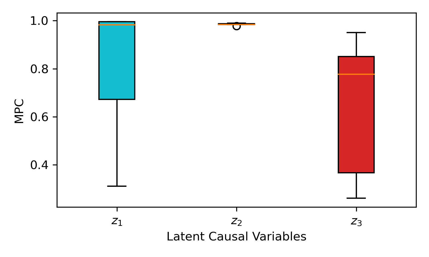
(a)

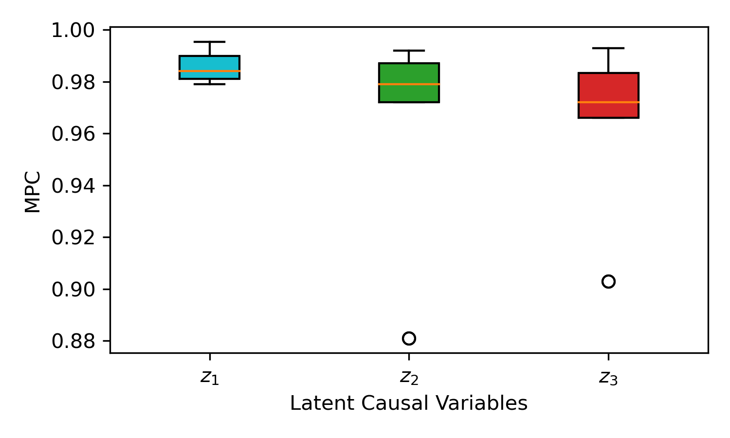
(b)

Figure 7: Performances of the proposed SuaVE in recovering the latent causal variables on Change 1 (a), and Change 2 (b).

The Figure 7 shows the MPC between the recovered latent variables and the true ones by the proposed SuaVE. For Change 1, we can see that only the recovered $z_{2}$ obtains satisfactory MPC. For Change 2, all the recovered latent causal variables obtain high MPC, which seems to be promising to obtain identifiability. To further understand this interesting result, we investigate the recovered graph in the case of Change 2. Again, we also use a threshold to remove some edges to obtain the final graph. Since no identifiability is provided, we measure the SHD of CPDAG. We found that for Change 2, the proposed method obtains SHD = 1.0 $\pm$ 0.39. Compared to that, we reported SHD = 0.6 $\pm$ 0.35 in Figure 5 where the weights always change across $\mathbf{u}$. Note that, the setting of Change 2 still meets the assumptions of Theorem 4.1, thus obtaining identifiability.

A.8 Experiments on i.i.d. $z_{i}$

As we mentioned in the main paper, our work is closely related to nonlinear ICA, and our assumptions includes the assumptions for identifying the Gaussian noise variables. To verify this point, we conduct experiments on the case where any two latent causal variables $z_{i}$ are independent given $\mathbf{u}$. Data details is the same as mentioned in section A.6.2, but we here enforce $\lambda_{i,j}(\mathbf{u})=0$ for each $i,j$. Again, the network architecture, optimization and hyper-parameters are the same as section A.6.2, except for learning rate (here we set $1r=1e-2$). Figure 8 shows the performances of the proposed SuaVE and iVAE. We can see that iVAE is slightly better than the proposed SuaVE, both obtain satisfying results in terms of MPC.

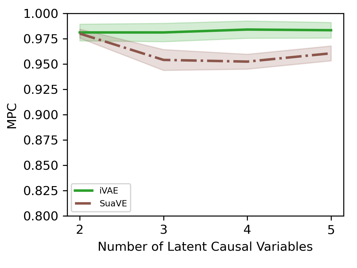
(a)

Figure 8: Performances of the proposed SuaVE and iVAE in recovering the independent latent causal variables conditional $\mathbf{u}$.

A.9 Detailed Results on fMRI

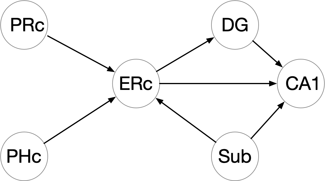
(a)

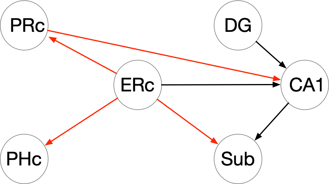
(b)

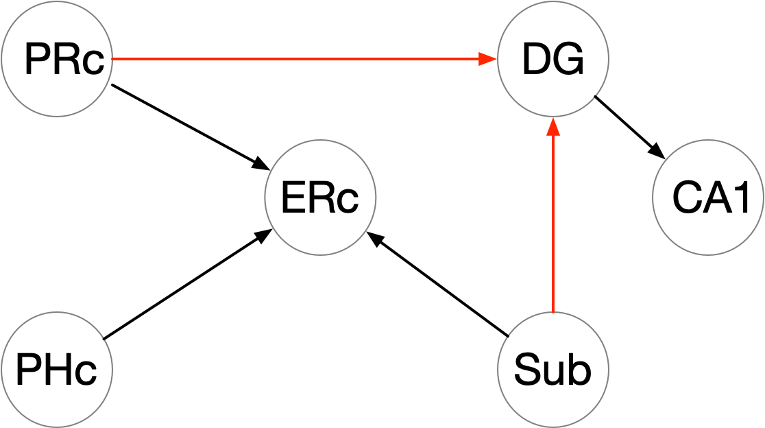
(c)

Figure 9: Recovered graphs on fMRI Data. (a) the anatomical connections given in Bird & Burgess (2008). (b) The recovered causal graph by the proposed SuaVE. (c) The recovered causal graph reported in (Ghassami et al., 2018). Note that the setting in (b) treats fMRI data as latent variables, while the setting in (c) treats fMRI data as observed variables.

Figure 9 (a) show the edges in the anatomical ground truth reported in (Ghassami et al., 2018). Figure 9 (b) show the latent recovered edges by the proposed SuaVE, in the setting where we treat fMRI data as latent causal variables. For comparison, Figure 9 (c) shows the recovered causal graph reported in (Ghassami et al., 2018), in the setting where fMRI data are treated as observed variables. That is, the setting in (b) is more challenging than the setting in (c).

Figure 10 shows the recovered latent six signals (Blue) and the true ones (Red) within one day by the proposed SuaVE.

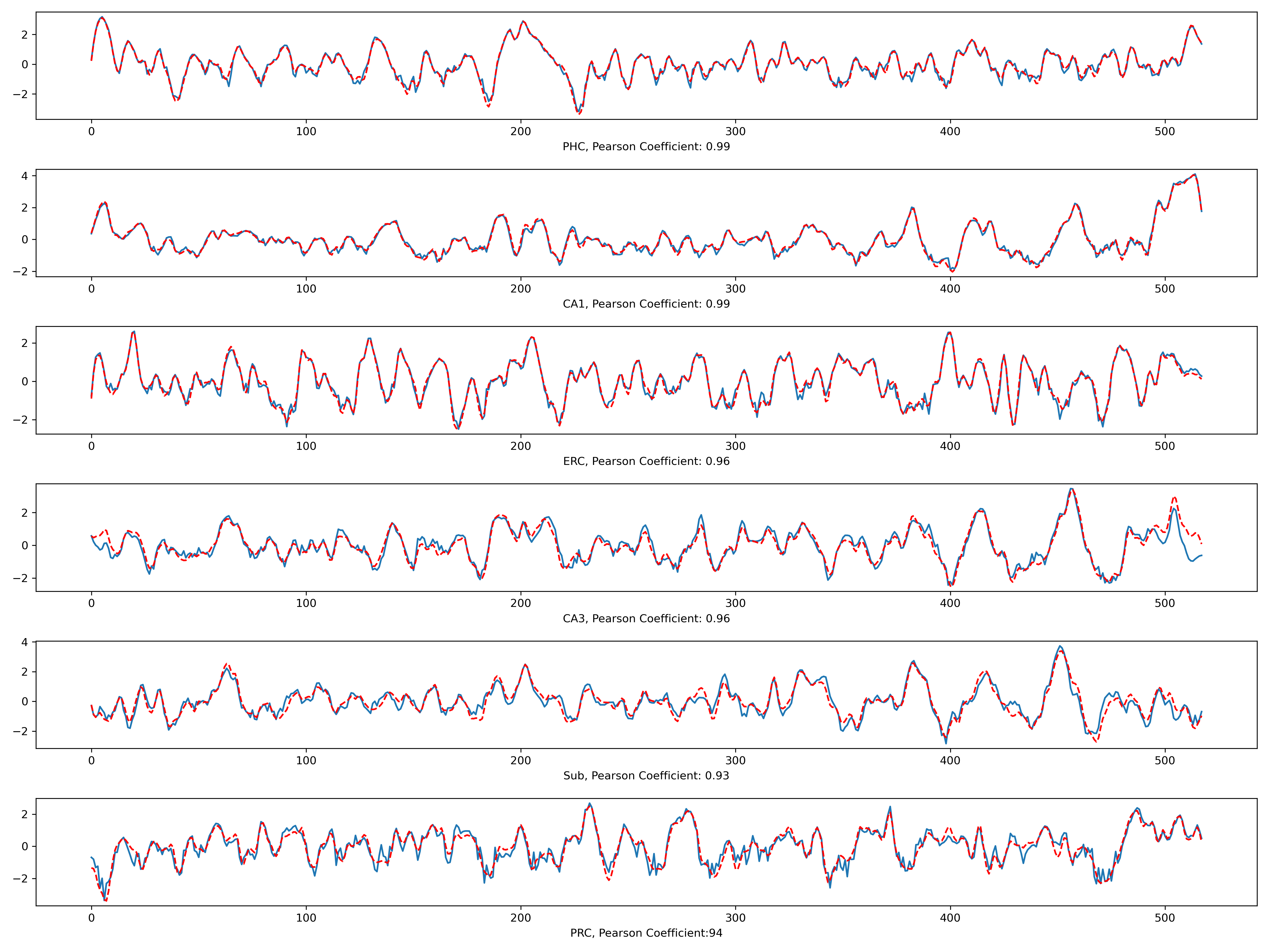
Figure 10: Recovered latent six signals (Blue) and the true ones (Red) within one day by the proposed SuaVE.

The recovered latent fMRI variables within one day by iVAE are depicted by Figure 11.

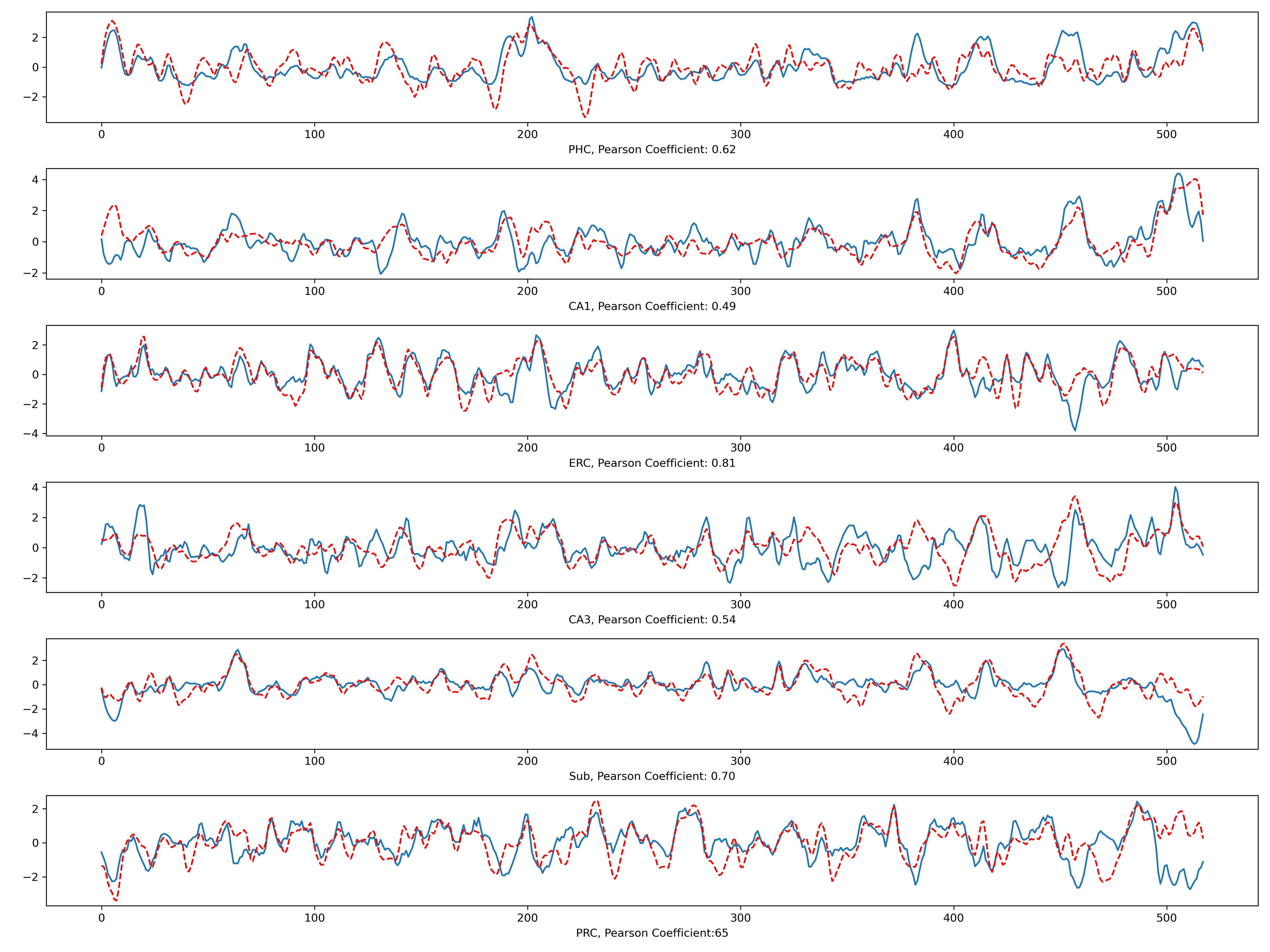
Figure 11: Recovered latent six signals (Blue) and the true ones (Red) within one day by iVAE.

The recovered latent fMRI variables within one day by VAE are depicted by Figure 12.

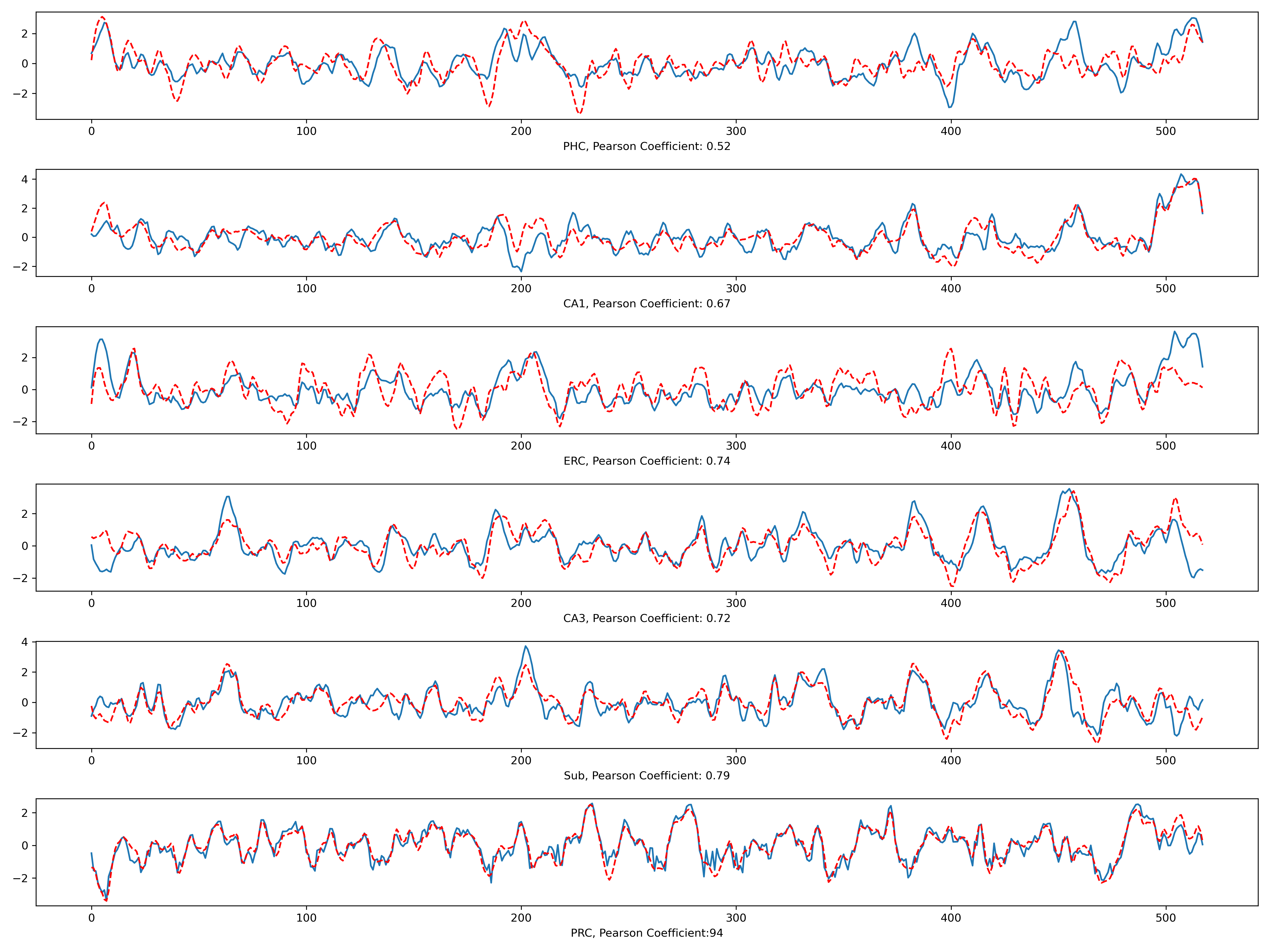
Figure 12: Recovered latent six signals (Blue) and the true ones (Red) within one day by VAE.

The recovered latent fMRI variables within one day by $\beta$-VAE are depicted by Figure 13.

The recovered latent fMRI variables within one day by CausalVAE are depicted by Figure 14.

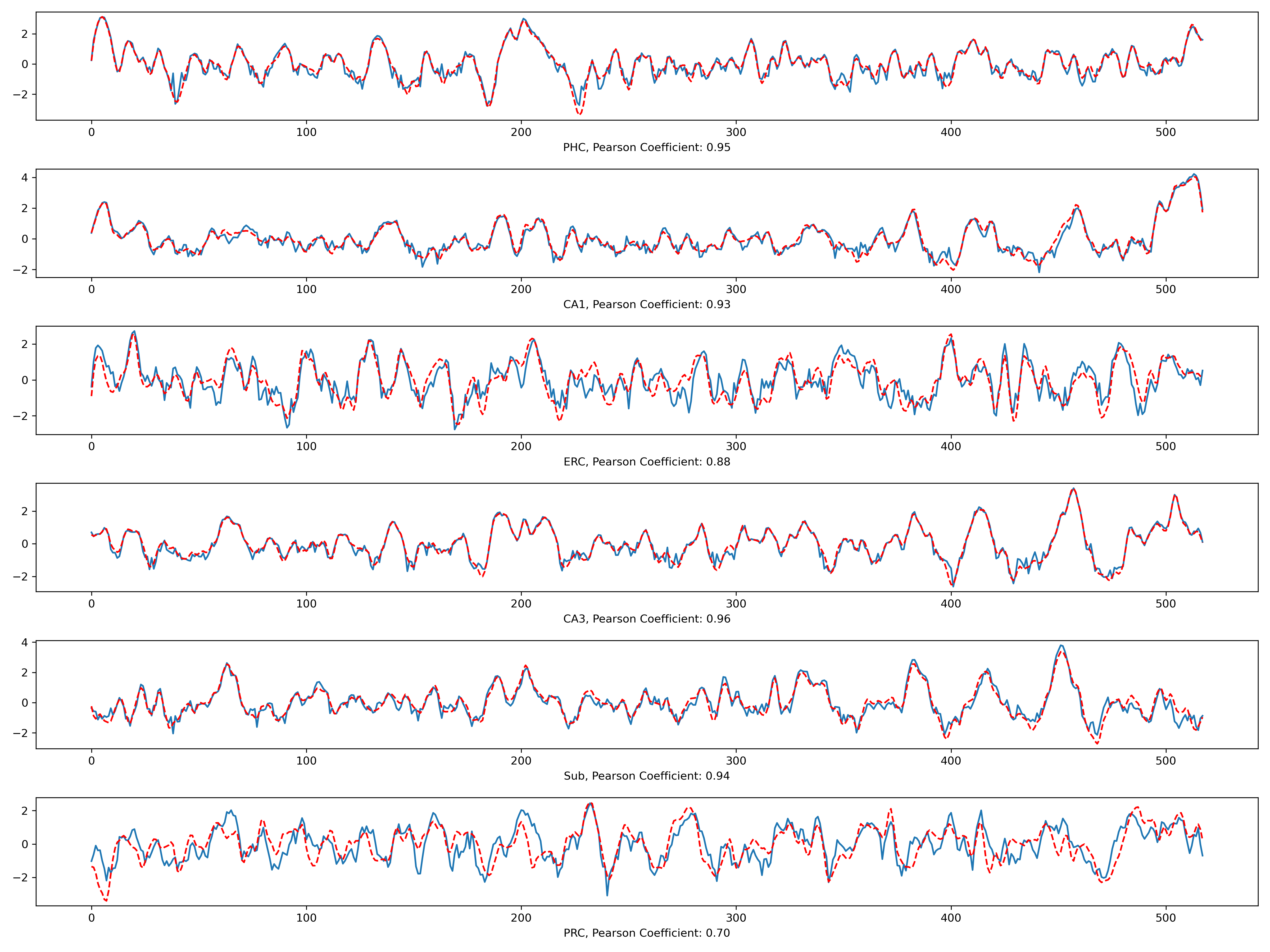
Figure 13: Recovered latent six signals (Blue) and the true ones (Red) within one day by $\beta$-VAE.

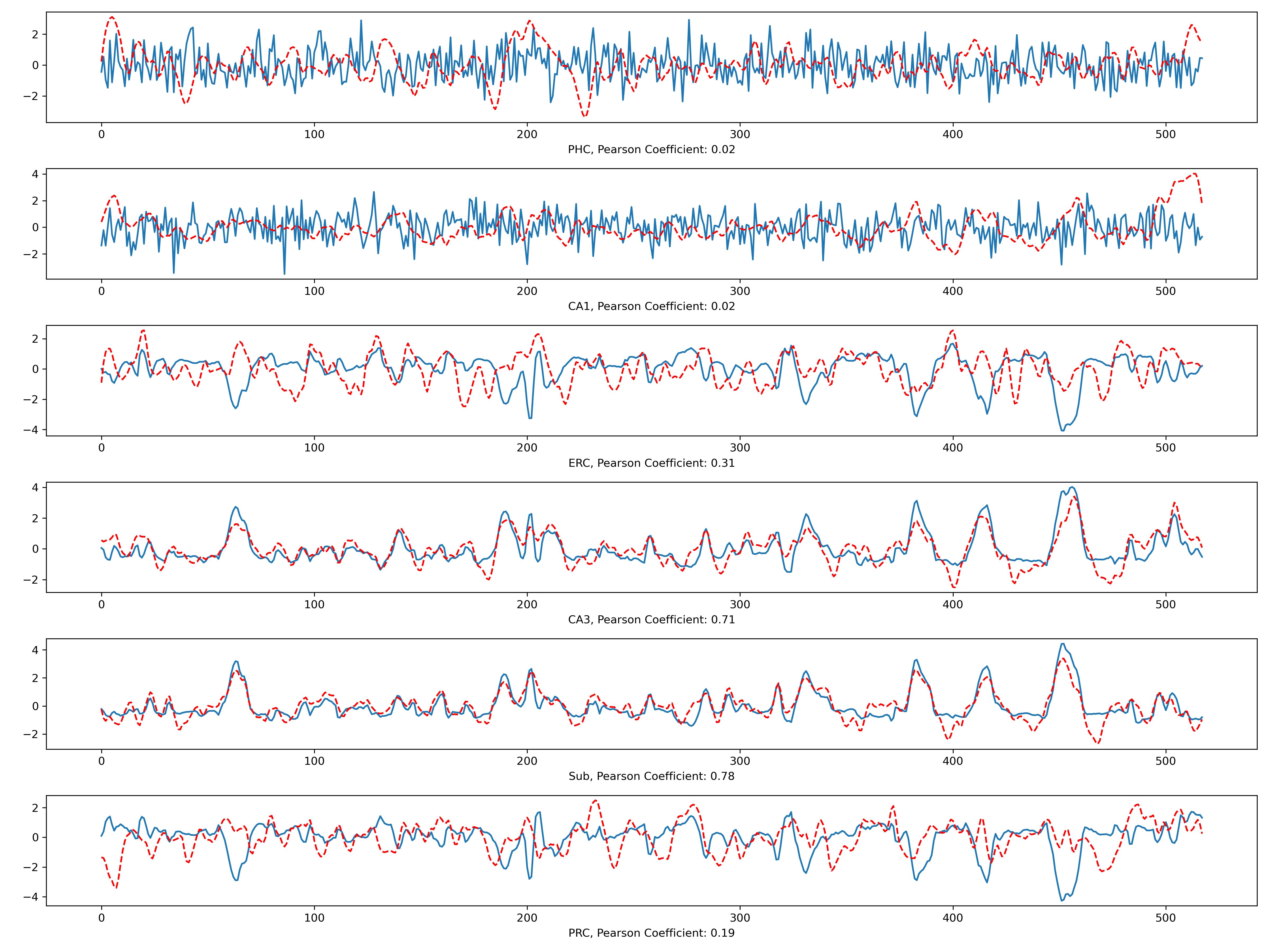
Figure 14: Recovered latent six signals (Blue) and the true ones (Red) within one day by CausalVAE.

Implementation Details: For fMRI data, again, we used the same network architecture for encoder (e.g. 3-layer fully connected network with 30 hidden nodes for each layer) and decoder (e.g. 3-layer fully connected network with 30 hidden nodes for each layer) parts in all these models. For prior model in the proposed SuaVE and iVAE, we use 3-layer fully connected network with 30 hidden nodes for each layer. We assign an 3-layer fully connected network with 30 nodes to generate the weights to model the relations among latent causal variables in the proposed SuaVE. For hyper-parameters, we set $\beta=4,25,50$ for $\beta$-VAE. For CausalVAE, we use the hyper-parameters setting as recommended by the authors (Yang et al., 2021), for generating observed $\mathbf{x}$, we use an invertible 2-layer multi-layer perceptron on the fMRI with different 5 random seeds.

References

- Adams et al. (2021) Adams, J., Hansen, N., and Zhang, K. Identification of partially observed linear causal models: Graphical conditions for the non-gaussian and heterogeneous cases. In NeurIPS, 2021.
- Anandkumar et al. (2013) Anandkumar, A., Hsu, D., Javanmard, A., and Kakade, S. Learning linear bayesian networks with latent variables. In ICML, pp. 249–257, 2013.
- Bengio et al. (2013) Bengio, Y., Courville, A., and Vincent, P. Representation learning: A review and new perspectives. IEEE TPAMI, 35(8):1798–1828, 2013.
- Bird & Burgess (2008) Bird, C. M. and Burgess, N. The hippocampus and memory: insights from spatial processing. Nature Reviews Neuroscience, 9(3):182–194, 2008.
- Bishop & Nasrabadi (2006) Bishop, C. M. and Nasrabadi, N. M. Pattern recognition and machine learning, volume 4. Springer, 2006.
- Brehmer et al. (2022) Brehmer, J., De Haan, P., Lippe, P., and Cohen, T. Weakly supervised causal representation learning. arXiv preprint arXiv:2203.16437, 2022.
- Cai et al. (2019) Cai, R., Xie, F., Glymour, C., Hao, Z., and Zhang, K. Triad constraints for learning causal structure of latent variables. In NeurIPS, 2019.
- Chen et al. (2018) Chen, R. T., Li, X., Grosse, R., and Duvenaud, D. Isolating sources of disentanglement in vaes. In NeurIPS, 2018.
- Frot et al. (2019) Frot, B., Nandy, P., and Maathuis, M. H. Robust causal structure learning with some hidden variables. Journal of the Royal Statistical Society: Series B (Statistical Methodology), 81(3):459–487, 2019.
- Ghassami et al. (2018) Ghassami, A., Kiyavash, N., Huang, B., and Zhang, K. Multi-domain causal structure learning in linear systems. Advances in neural information processing systems, 31, 2018.
- Higgins et al. (2017) Higgins, I., Matthey, L., Pal, A., Burgess, C. P., Glorot, X., Botvinick, M., Mohamed, S., and Lerchner, A. beta-vae: Learning basic visual concepts with a constrained variational framework. In ICLR, 2017.
- Huang et al. (2019) Huang, B., Zhang, K., Gong, M., and Glymour, C. Causal discovery and forecasting in nonstationary environments with state-space models. ICML, 2019.
- Huang* et al. (2020) Huang*, B., Zhang*, K., Zhang, J., Ramsey, J., Sanchez-Romero, R., Glymour, C., and Schölkopf, B. Causal discovery from heterogeneous/nonstationary data. JMLR, 21(89), 2020.
- Hyvarinen et al. (2019) Hyvarinen, A., Sasaki, H., and Turner, R. Nonlinear ica using auxiliary variables and generalized contrastive learning. In The 22nd International Conference on Artificial Intelligence and Statistics, pp. 859–868. PMLR, 2019.
- Khemakhem et al. (2020) Khemakhem, I., Kingma, D., Monti, R., and Hyvarinen, A. Variational autoencoders and nonlinear ica: A unifying framework. In AISTAS, pp. 2207–2217. PMLR, 2020.
- Kim & Mnih (2018) Kim, H. and Mnih, A. Disentangling by factorising. In ICML, 2018.
- Kingma & Welling (2013a) Kingma, D. P. and Welling, M. Auto-encoding variational bayes. NeurIPS, 2013a.
- Kingma & Welling (2013b) Kingma, D. P. and Welling, M. Auto-encoding variational bayes. arXiv preprint arXiv:1312.6114, 2013b.
- Kingma et al. (2016) Kingma, D. P., Salimans, T., Jozefowicz, R., Chen, X., Sutskever, I., and Welling, M. Improved variational inference with inverse autoregressive flow. In NeurIPS, volume 29, pp. 4743–4751, 2016.
- Kivva et al. (2021) Kivva, B., Rajendran, G., Ravikumar, P., and Aragam, B. Learning latent causal graphs via mixture oracles. NeurIPS, 2021.
- Kocaoglu et al. (2018) Kocaoglu, M., Snyder, C., Dimakis, A. G., and Vishwanath, S. Causalgan: Learning causal implicit generative models with adversarial training. In ICLR, 2018.
- Koller & Friedman (2009) Koller, D. and Friedman, N. Probabilistic graphical models: principles and techniques. MIT press, 2009.
- Lachapelle et al. (2021) Lachapelle, S., López, P. R., Sharma, Y., Everett, K., Priol, R. L., Lacoste, A., and Lacoste-Julien, S. Disentanglement via mechanism sparsity regularization: A new principle for nonlinear ica. arXiv preprint arXiv:2107.10098, 2021.
- Laumann & Poldrack (2015) Laumann, T. O. and Poldrack, R. A., 2015. URL https://openfmri.org/dataset/ds000031/.
- Lippe et al. (2022) Lippe, P., Magliacane, S., Löwe, S., Asano, Y. M., Cohen, T., and Gavves, S. Citris: Causal identifiability from temporal intervened sequences. In International Conference on Machine Learning, pp. 13557–13603. PMLR, 2022.
- Locatello et al. (2019) Locatello, F., Bauer, S., Lucic, M., Raetsch, G., Gelly, S., Schölkopf, B., and Bachem, O. Challenging common assumptions in the unsupervised learning of disentangled representations. In ICML, 2019.
- Locatello et al. (2020) Locatello, F., Poole, B., Rätsch, G., Schölkopf, B., Bachem, O., and Tschannen, M. Weakly-supervised disentanglement without compromises. In ICML, 2020.
- Maaløe et al. (2019) Maaløe, L., Fraccaro, M., Liévin, V., and Winther, O. Biva: A very deep hierarchy of latent variables for generative modeling. In NeurIPS, 2019.
- Pearl (2000) Pearl, J. Causality: Models, Reasoning, and Inference. Cambridge University Press, Cambridge, 2000.
- Peters et al. (2014) Peters, J., Mooij, J. M., Janzing, D., and Schölkopf, B. Causal discovery with continuous additive noise models. JMLR, 15(58):2009–2053, 2014.
- Peters et al. (2017) Peters, J., Janzing, D., and Schlkopf, B. Elements of Causal Inference: Foundations and Learning Algorithms. The MIT Press, 2017.
- Schölkopf et al. (2021) Schölkopf, B., Locatello, F., Bauer, S., Ke, N. R., Kalchbrenner, N., Goyal, A., and Bengio, Y. Toward causal representation learning. Proceedings of the IEEE, 109(5):612–634, 2021.
- Shimizu et al. (2009) Shimizu, S., Hoyer, P. O., and Hyvärinen, A. Estimation of linear non-gaussian acyclic models for latent factors. Neurocomputing, 72(7-9):2024–2027, 2009.
- Silva et al. (2006) Silva, R., Scheines, R., Glymour, C., Spirtes, P., and Chickering, D. M. Learning the structure of linear latent variable models. JMLR, 7(2), 2006.
- Sønderby et al. (2016) Sønderby, C. K., Raiko, T., Maaløe, L., Sønderby, S. K., and Winther, O. Ladder variational autoencoders. In NeurIPS, 2016.
- Sorrenson et al. (2020) Sorrenson, P., Rother, C., and Köthe, U. Disentanglement by nonlinear ica with general incompressible-flow networks (gin). arXiv preprint arXiv:2001.04872, 2020.
- Spirtes et al. (2001) Spirtes, P., Glymour, C., and Scheines, R. Causation, Prediction, and Search. MIT Press, Cambridge, MA, 2nd edition, 2001.
- Träuble et al. (2021) Träuble, F., Creager, E., Kilbertus, N., Locatello, F., Dittadi, A., Goyal, A., Schölkopf, B., and Bauer, S. On disentangled representations learned from correlated data. In ICML, pp. 10401–10412. PMLR, 2021.
- Vahdat & Kautz (2020) Vahdat, A. and Kautz, J. Nvae: A deep hierarchical variational autoencoder. In NeurIPS, 2020.
- Von Kügelgen et al. (2021) Von Kügelgen, J., Sharma, Y., Gresele, L., Brendel, W., Schölkopf, B., Besserve, M., and Locatello, F. Self-supervised learning with data augmentations provably isolates content from style. In Advances in neural information processing systems, 2021.
- Xie et al. (2020) Xie, F., Cai, R., Huang, B., Glymour, C., Hao, Z., and Zhang, K. Generalized independent noise condition for estimating latent variable causal graphs. In NeurIPS, 2020.
- Xie et al. (2022) Xie, F., Huang, B., Chen, Z., He, Y., Geng, Z., and Zhang, K. Identification of linear non-gaussian latent hierarchical structure. In International Conference on Machine Learning, pp. 24370–24387. PMLR, 2022.
- Yang et al. (2021) Yang, M., Liu, F., Chen, Z., Shen, X., Hao, J., and Wang, J. Causalvae: Structured causal disentanglement in variational autoencoder. In CVPR, 2021.
- Yao et al. (2021) Yao, W., Sun, Y., Ho, A., Sun, C., and Zhang, K. Learning temporally causal latent processes from general temporal data. arXiv preprint arXiv:2110.05428, 2021.
- Yao et al. (2022) Yao, W., Chen, G., and Zhang, K. Learning latent causal dynamics. arXiv preprint arXiv:2202.04828, 2022.
- Zhang & Hyvarinen (2012) Zhang, K. and Hyvarinen, A. On the identifiability of the post-nonlinear causal model. arXiv preprint arXiv:1205.2599, 2012.
- Zheng et al. (2018) Zheng, X., Aragam, B., Ravikumar, P., and Xing, E. P. Dags with no tears: Continuous optimization for structure learning. In NeurIPS, 2018.