A theoretical review on the single-impurity electron spin resonance on surfaces
Abstract
The development of electron spin resonance (ESR) combined with scanning tunneling spectroscopy (STM) is undoubtedly one of the main experimental breakthroughs in surface science of the last decade thanks to joining the extraordinarily high energy resolution of ESR (nano-eV scale) with the single-atom spatial resolution of STM (sub-Ångström scale). While the experimental results have grown with the number of groups that have succeeded in implementing the technique, the physical mechanism behind it is still unclear, with several different mechanisms proposed to explain it. Here, we start by revising the main characteristics of the experimental setups and observed features. Then, we review the main theoretical proposals, with both their strengths and weaknesses. One of our conclusions is that many of the proposed mechanisms share the same basic principles, This explains why these mechanims are essentially equivalent in a broad picture. We analyze the subtle differences between some of them and how they compare with the different experimental observations.
keywords:
STM, magnetic-resonance , spin , adatoms , drivingPACS:
72.15.Qm , 75.10.Jm , 75.30.GW , 75.30.Hx , 75.78.-n , 76.20.+q1 Introduction
Electron spin resonance (ESR, also known as electron paramagnetic resonance -EPR) and nuclear magnetic resonance (NMR) are two of the most successful and broadly used characterization and imaging techniques, employed from medical and bio applications to chemical characterization of paramagnetic complexes [1]. Among their strengths, they provide a high-energy resolution of magnetic transitions even in ambient conditions, limited basically by the time the wave functions preserve their phase, known as the phase decoherence time , and non-invasive and non-destructive measurement, ideal for in-vivo applications. The spatial resolution of these techniques is essentially limited by the magnetic field gradients that can be implemented. Presently this implies commercial equipments [2] capable of spatial resolutions of the order of 100 m3. While these resolutions can be enough for biomedical imaging applications, a higher spatial resolution is desirable for surface and chemical analysis, such as the one needed in quality assessment of thin-layer industrial applications (hard drives, magnetic tunnel junctions for sensing applications, etc). NMR with nm3 spatial resolution has been demonstrated by optical means using a nitrogen-vacancy center in a nanodiamond at the tip apex of atomic force microscope (AFM) [3] or, more recently, NV-center layer at the surface of a diamond chip [4].
Early attempts of ESR implemented on an STM (STM-ESR) used a radiofrequency rotating magnetic field to modulate the static magnetic field. When the central frequency of the narrow detection band equaled the frequency of the signal, the detector showed a signal until the magnetic-field modulation frequency was out of the detection band. These initial attempts demonstrated the presence of resonant magnetic field-dependent features, revealed as an increased noise in the tunnel current at the spin precession frequency [5, 6]. Unfortunately, difficulties some of the experimental variables made the results sometimes irreproducible and unclear.
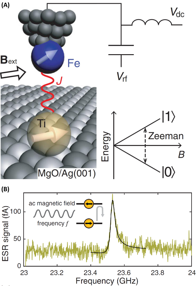
All-electrical ESR with atomic spatial resolution has been a long-standing goal of the surface science community. The use of a radiofrequency-driven electric field renders the technique more simple to achieve. In 2014, Müllegger et al. reported STM-ESR and NMR [7] of a terbium-double decker molecule (TbPc2) residing inside the STM tunnel junction formed by the tip and an Au(111) substrate, and they argued that the observed features of the resonance did not satisfy well-established dipole selection rules () for the magnetic resonance [8]. Baumann et al. [9] provided the first conclusive and fully-reproducible results of STM-ESR of single atoms. Among the many experimental challenges that Baumann et al. had to solve to achieve this reproducibility, the full characterization and compensation of the frequency-dependent transmission function of the STM junction was a key technical point. Since then, a plethora of experimental results of STM-ESR has appeared [9, 10, 11, 12, 13, 14, 15, 16, 17, 18, 19, 20, 21, 22, 23], demonstrating the STM-ESR with a resolution capable of revealing hyperfine interactions on single transition-metal atoms deposited on MgO [24]. This technique has shown remarkable achievements such as the unambiguous measurement of the magnetic moment of a single -electron atom [10], the differentiation of individual Ti atoms by their number of nucleons [14], or the full characterization of the spin interaction between two adatoms [11, 18] among others.
These all-electric STM-ESR works use a high-end radiofrequency generator to modulate the applied bias between tip and sample, see Fig. 4. Another successful approach uses a second macroscopic electrode positioned at milli-meters from the STM tip, working as a radiofrequency antenna [25, 20]. Within the available data, these different approaches seem capable of the same achievements.
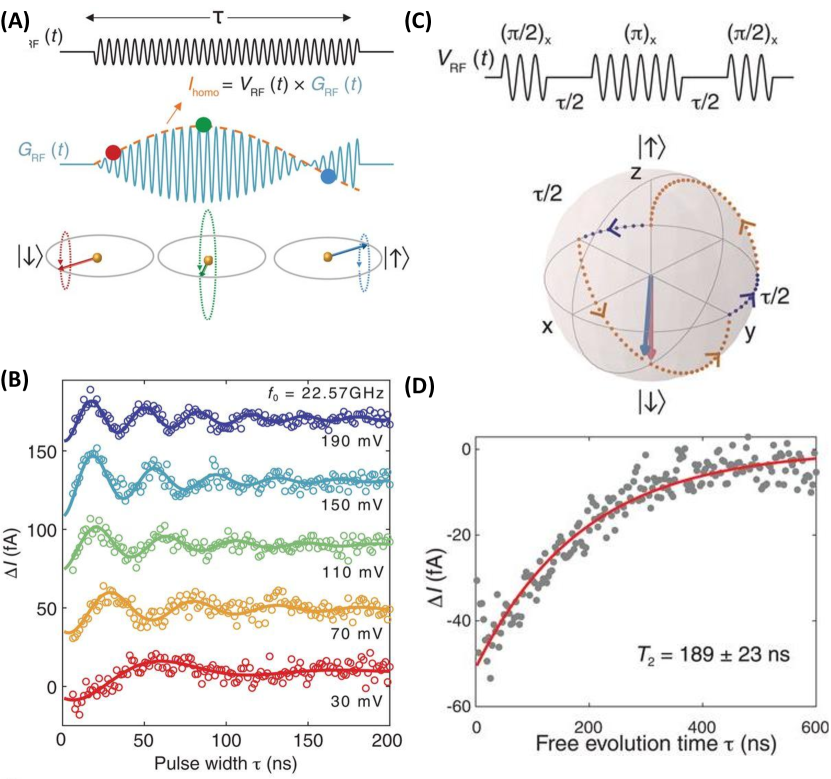
The above results show the spectroscopic capabilities of continuous-wave STM-ESR. Indeed, the long-time average under a continuous sinusoidal driving of the tip-sample electric field is an efficient way of revealing Rabi oscillations between local spin states. Beyond spectroscopy obtained in the continuous-wave mode, it is interesting to do STM-ESR with microwave pulses. Pulses of radiation interacting with single spins are at the core of quantum operations [26, 27, 28]. Recently, pulses of radiofrequencies were mastered in the STM-ESR [19], which paves the way for coherent manipulation of single spins with atomic resolution, see Fig. 2.
Understanding the actual driving mechanisms of local spins in the STM junction is not easy. For a comprehensive review on the theoretical approaches trying to explain the early experiments by Mannassen et al., see the work of Balatsky et al. [6]. In essence, the possible mechanism lies into two non-mutually exclusive classes: those works that rely on the spin-orbit coupling to explain the interaction between the local spin and the tunnel current, or those where such a coupling is not demanded, such as the direct exchange mechanism based on a tunnel barrier modulation. Here, we will instead focus on the theory of all-electrical STM-ESR
Direct estimations of the radiofrequency magnetic field created by the alternating tunnel current [18] or the radiofrequency antenna [25] displacement current permit us to discard this straightforward origin. Moreover, recent measurements of the STM-ESR dependence on the standoff tip-sample distance are not compatible with the dependence of these radiofrequency current-mediated mechanisms [20].
A different mechanism based on a radiofrequency current-induced magnetic field was proposed [29], where the spin-polarized current was driving finite uniaxial and transverse anisotropy fields on the local spin moment. However, this mechanism predicts null ESR signal on half-integer spins, such as the spin-1/2 STM-ESR on Ti that was observed later [13, 14, 15, 17, 18, 19, 25, 20, 21, 22, 23].
The piezoelectric displacement of the adatom produced by the radiofrequency electric field in the STM junction is at the origin of several proposed mechanism. Baumann et al. [9] argue that this piezoelectric vibration of the adatom produces a modulation of the single-ion magnetic anisotropy, which is seen in the spin-polarized DC tunnel current thanks to its magnetoresistive dependence. Another mechanism associated with the piezoelectric displacement is the modulation of the exchange and dipolar magnetic fields created by the tip [30, 20]. Additionally, for certain systems, the modulation of the -factor due to the variation of the crystal field felt by the local moment may be sufficient to explain the ESR signal [31]. These mechanisms will be discussed in Sec. 3.1. Furthermore, there is additional mechanism that does not need to be related to the piezoelectric coupling, but can be strongly enhanced by the piezoelectric response of the substrate. This mechanism is based on the modulation of the tunneling probability by the applied alternating bias voltage. This modulation can stand on either a piezoelectric deformation of the tunnel barrier, and thus, a variation of the effective barrier width, or a change in the barrier height associated with the alternating bias established at the STM junction. In both cases, its effect on the DC tunnel current can be taken into account by a time-dependent description of the cotunneling processes [32]. To end this list, we mention a different proposal based on the time-dependent spin-torque produced by the spin-polarized tunnel current [33].
All-electric STM-ESR has been very successful on local magnetic moments adsorbed on a bilayer of MgO grown on Ag (100). To the best of our knowledge, this is the only substrate that has led to ESR-active atomic and molecular adsorbates. The strong piezoelectric response of MgO layers is a good indication of the importance of mechanical vibrations induced by the oscillating electric field of the tip in the ESR mechanism. However, as emphasized by the cotunneling approach, the ultimate origin may be the way the tunneling properties change with the applied electric field. This modulation can be greatly enhanced by the piezoelectric response of the substrate, but it is in principle independent of it. This fact implies that all-electric STM-ESR should be possible on a number of substrates besides MgO.
The structure of this article is a first section reviewing qualitative aspects of STM-ESR together with the figures of merit governing the spin-resonance process. Next, we review the different proposals for the mechanisms behind STM-ESR. Followed by a section analyzing common and specific features. The article ends with a summary and conclusions section. Several appendices give more details on the derivations of the involved theories.
2 Basics of STM-ESR. Figures of merit.
Electron spin resonance is a technique based on exciting a Rabi oscillation between two magnetic levels in an electronic system. It is then important to understand Rabi oscillations between two levels. In this section, we give a brief overview of the driven two-level system (TLS) and the figures of merit that characterizes the stationary dynamics, typically obtained as long-time averages. As we mentioned in the Introduction, the specificities of STM-ESR is to use an all-electric technique to drive a single atomic or molecular spin system in an STM junction. Besides driving the spin, we need to detect it. The ESR signal translates into a change in electronic current when either the frequency of the driving bias voltage [9] or of the radiofrequency field created by a microantenna [20] matches the Larmor frequency of the TLS. In this section, we briefly review these concepts and how they apply to the STM-ESR case.
2.1 Driven spin system: the Rabi frequency
A key ingredient in ESR is the Rabi frequency, also known as Rabi flop rate. Just by understanding and evaluating this quantity, much insight can be gained in the resonant excitation of a spin. We briefly review its definition and meaning in the context of the dynamics of the driven TLS.
2.1.1 The TLS
The magnetic resonance of a quantum system can be described exactly in the same way as standard ESR or nuclear magnetic resonance (NMR), and it is formally equivalent to an optically driven system [45]. To begin with, let us assume that a quantum system described by a Hamiltonian is subjected to a time-dependent field oscillating at an angular frequency . Due to this time-dependent interaction, we assume that only two states and with eigenenergies and of the unperturbed are connected by a transition frequency111In the context of magnetic resonance of a spin system, this will be the Larmor frequency , with the electronic gyromagnetic factor close enough to the driving frequency . Under these conditions, the driven isolated system can be treated as a TLS. Thus, we will concentrate on the time evolution on the subspace of dimension two spanned by and . If the radiative shifts of levels and are included in the frequency , we can write the driven system Hamiltonian as
| (1) | |||||
where is the -Pauli matrix in the basis set and is called the Rabi frequency, which characterizes the strength of the driving.
To get some further insight, let us consider the stationary case with . If the system is initially prepared in state , the state at time will be given by
| (2) |
In other words, the state of the system will oscillate coherently between and at a frequency (the probabilities or state populations oscillate at ).
The dynamics of the driven system (1) is certainly more complex. In disentangling the role of the Rabi frequency, it is convenient to write the driving term as
| (3) |
where we have defined and . Thus, the driving term contains resonant processes where the system is excited by the absorption of a photon (or decay by the emission of a photon), the first two terms in Eq. (3), and non-resonant processes where it is excited after emitting a photon (or it decays after absorbing a photon), the last two terms in Eq. (3) [45]. These last two non-resonant processes are very unlikely and can be then neglected. This constitutes the rotating-wave approximation (RWA). Hence, the driving term under the RWA takes the form .
The main benefit of the RWA is that it permits describing the system dynamics in a rotating frame where the time-dependence can be removed. In particular, by applying the transformation to the rotation frame defined by , we get that the Hamiltonian is transformed according to , so that
| (4) |
where . This Hamiltonian can be easily diagonalized to obtain the two eigenvalues, , where is known as the generalized Rabi frequency. This result allows us to interpret the Rabi frequency in quite simple terms. When the system is driven by a quasi-resonant perturbation of intensity , its state coherently oscillates at in a frame rotating around the -axis of Hamiltonian (1) at frequency , very much like in Eq. (2). In particular, at resonance (), it will oscillate at half the Rabi frequency , i.e., the state will oscillate between states and at a frequency determined by the strength of the driving.
The proposed mechanism for STM-ESR must be such that the Rabi frequency matches the experimental one. A system will be ESR-active if we have sizeable Rabi frequencies.
2.1.2 Bloch equations for the TLS
The time evolution of the isolated system will be determined by the Schrödinger equation , or equivalently, by the coherent evolution of its density matrix, . Let us now consider a very large system composed by our quantum system, characterized by a Hamiltonian , and the rest, which we will call reservoirs. In particular, we will be interested in the limit where the reservoirs are very large systems with quasi-continuum spectra, in other words, thermal baths that will remain in thermal equilibrium. If is the complete many-body time-dependent state of the full system, the density matrix of the whole system will be . Since in general we are interested only in the evolution of our quantum system, we can disregard most of the information of the baths. Hence, it is particularly useful to trace out the degrees of freedom of the reservoirs by introducing the reduced density matrix of the system:
| (5) |
where indicates the trace over the bath degrees of freedom, . The reduced density matrix can be used to describe the evolution of the system coupled to its environment, but the price to pay is that the Heisenberg equation of motion of will contain, in addition to the coherent part , a very complex dissipative part accounting for the coupling with the baths. This is done by including a super-operator called the Liouvillian, see for example Ref. ([46]). In general, such a problem cannot be solved, and further approximations are needed. Fortunately, in many cases, the coupling of the quantum system with its environment can be considered weak, so a second-order perturbative treatment on this coupling is sufficient. In addition, the bath correlation time is often very short, much shorter than any other characteristic time scale of the system, which allows us to neglect memory effects. This is known as the Markovian approximation. Under these conditions, one can derive a Bloch-Redfield master equation for where the Liouvillian takes the form of the time-independent Lindblad super-operators [46].
In order to derive the main equations controlling the ESR, we will use the standard approximation employed to derive the optical Bloch equations for the two level system [45]. As such, we will assume a relaxation rate and a decoherence rate independent of the driving field. This approximation is valid if the effect of this radiation can be neglected during the correlation time of the vacuum fluctuations responsible for the spontaneous emission, which holds if [45]. In addition, we limit the discussion to the TLS under the RWA where fast oscillating terms, at frequencies , are neglected.
and as spins down and up respectively. Then, we can identify [47] the quantities , and , and splitting the real and imaginary parts by introducing and , we get the following dynamical equations[45]
| (6) | |||||
| (7) | |||||
| (8) |
where is the thermal equilibrium value of . Equations (8) are equivalent to the macroscopic dynamical equations for the magnetization dynamics in ESR or NMR described in a rotating frame [1], see Fig. 3. In particular, the steady state solution of these effective spin components are given by
| (9) | |||||
| (10) | |||||
| (11) |
where .
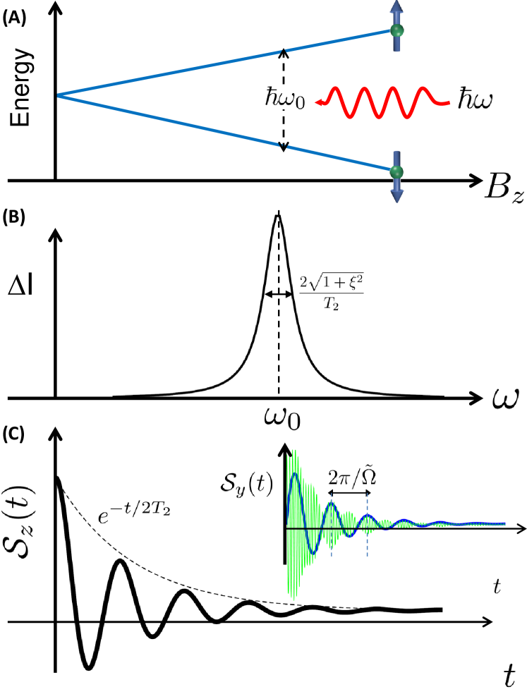
The dynamics of the TLS in the steady-state or at long times are then completely controlled by three quantities proper to the TLS and its environment: the Rabi frequency, , the relaxation time, , and the decoherence time, . The meaning of the two relaxation times, and , can be easily derived from (8). is de exponential decline of the population difference. It is indeed a relaxation time towards its equilibrium value. controls the non-diagonal terms of the density matrix (coherences) account for the relative phase between the states of . This phase is destroyed if an event introduces a random phase in one of the wavefunction components, like scattering with an external particle. This is a purely dephasing event, and it is usually assigned a pure-dephasing rate . But of course, destroying the population of one of the state also leads to losing the coherence between states. Then the decoherence rate of a TLS is given by
| (12) |
Depending on the actual parameters of the system, the dynamics of the populations can actually vary. For the Fig. 3, we find that the difference in populations or longitudinal magnetization, , actually decays as . This type of dependence of the population difference on the decoherence rate has been explored in Ref. ([48]).
In summary, these three numbers, , and , control the features of continuous-wave ESR where the driving is a single harmonic function of time. Typical figures for experiments on a Fe adatom on MgO/Ag(100) [9, 12] are s-1, s, s. We see that decoherence dominates the evolution. Indeed, of the tunneling electrons cause decoherence [12] of the spin of Fe.
2.2 Detection mechanism of STM-ESR
In STM-ESR, the magnetic resonance is measured through the tunneling magnetoresistance effect at the STM junction. This means that the junction conductance depends on the relative alignment between the tip magnetic moment, and the precessing adatom spin, i.e., a contribution proportional to , where is the magnetic moment of the tip. Hence, it is not surprising that the change in the tunnel current between the RF on and RF off follows the frequency dependence of in Eq. (11) [9].
The DC current can be written in terms of the tunnel rates defined as the transition rate between the and states of the magnetic atom ( and if we stick to the TLS approximation) when an electron from the tip (surface) is scattered to the surface (tip). If we write the voltage and frequency-dependent occupation of the state as , the tunnel current can be written as
| (13) |
The occupations will differ in general from the thermal equilibrium ones, and they will be given by the stationary solution of the dynamical equation of the density matrix, i.e., . Using the solution of the Bloch equations for the TLS, Eq. (11), one can write the occupation difference between the two states connected by the ESR [50, 32]
| (14) |
where and will be given by the non-equilibrium occupation difference in the absence of RF modulation. In the case of a TLS, a closed expression of the tunnel current can be obtained with given by the thermal equilibrium occupation difference between the and states.
Let us consider the experimentally relevant case where a large DC bias voltage is applied (). Under these conditions, . In addition, we will assume a dominant elastic contribution to the current, , which is quite frequently found in spin-polarized STM experiments [51]. Then, by introducing the expectation value of the spin state, and the quantity , where is the direct spin-independent tunneling coupling and the tunneling exchange coupling (also known as the potential and exchange scattering matrix elements respectively), the change in tunneling current is
| (15) |
where is the tip polarization and the junction elastic conductance. Notice that since is the excited state, , so () when the tip and the adatom magnetic moment are aligned (antialigned). In other words, we can expect a deep (peak) in the DC tunnel current for the aligned (antialigned) tip polarization when the resonant condition is satisfied.
Equation (15) clearly illustrates the detection mechanism. The DC current is the non-equilibrium induced adatom magnetic moment and the tip moment ), which explains by STM-ESR is not observed in the absence of spin-polarization.
Experimental data of STM-ESR under larger RF voltages [18, 20, 25, 12] and/or larger tunnel conductances [16] shows important deviation from the symmetric frequency profile derived from Eq. (15). This asymmetric line shape has been explained in terms of the homodyne contribution to the DC current [13, 15, 19] (homodyne refers to processes happening at the same frequency). In the present context, there is a new contribution to the long-time average or DC current due to the RF component of the applied bias voltage. The symmetric contribution is due to the above magnetoresistive mechanism that yields a change in current with precessing frequency for a DC applied bias voltage. The homodyne contribution is, however, due to time-dependent tunneling conductance associated with the spin precession when it matches the RF applied bias, and it is responsible the appearance of an asymmetric Fano-like profile with frequency. In essence, the measured sinusoidal lock-in signal contains an approximately linear background as a function of the driving frequency that depends on both the Rabi frequency and the junction conductance. In the case of continuous STM-ESR, the resulting amplitude of the ESR signal close to resonance can be written as [15, 20]
| (16) |
where is a background contribution that accounts for the non-linearity of the junction, is the angle between the tip magnetic moment and the rotating magnetic moment, and defines the amplitude of the ESR signal, given by the equivalent of Eq. (15) for the total current,
| (17) |
Here we have introduced the saturation current as measured experimentally [15], while the phase shift between the RF excitation and the local spin has been neglected [20].
Interestingly, Eq. (16) contains both a symmetric contribution associated to the tunneling magnetoresistance () and the asymmetric homodyne contribution (). Thus, the resonance profile can be characterized by three quantities [20]: the amplitude , the width (we recall that ) and the asymmetry of the profile controlled by .
Interestingly, one can explain the asymmetric line shape without resorting to the homodyne detection scheme. G. Shavit et al. [52] demonstrated that the origin of the deviations from the symmetric line shape stands on the frequency dependences of the dissipative dynamics neglected in the derivation of the Bloch equations. By using a series of unitary transformations of the system Hamiltonian and avoiding the usual secular approximation with regard to the low-frequency Rabi frequency, they derived the asymmetric line shape (16). Moreover, their approach allowed them to account for the signal asymmetry sign depending on the applied bias, magnetic field orientation, and driving amplitude. This more involved approach does not contradict the above results. It rather goes beyond the simplifications above to express in a succinct formulation the same physics.
3 Proposed driving mechanism
3.1 Piezoelectric response
The piezoelectric displacement of the adatom driven by the radio frequency (RF) tip-induced electric field is at the core of several mechanisms proposed to explain the STM-ESR. For instance, the original mechanism based on the modulation of the crystal field [9] relies on this piezoelectric effect. In particular, for the 4-fold symmetric Fe/MgO/Ag system, Baumann and coworkers argue that the Rabi oscillations were proportional to [9]
| (18) |
Here, is a crystal field parameter mixing the orbitals states that differs in four units of orbital angular momenta. The basic principle behind this expression is the following. The radiofrequency voltage induces a displacement of the surface-adatom distance, much smaller than the equilibrium tip-adatom distance . Then, this change gives place to a RF modification of the crystal field parameter . Although the proposed mechanism correctly reproduces the magnetic field dependence of the Rabi flop rate for the Fe/MgO/Ag system [9, 10, 11, 12, 14, 16, 20, 21], it fails to explain the observed resonances on other adatoms, such as the Ti-H () [13, 14, 15, 17, 18, 19, 25, 20, 21, 22, 23]or the NMR of Cu [24].
In addition to the renormalization of the crystal field parameters due to the piezoelectric displacement, this oscillation modifies the exchange coupling between the adatom spin and the itinerant electrons [30]. The coupling with both tip and surface electrons is then modified, and thus, the tunneling-related exchange coupling. In particular, the finite tip magnetic moment can give place to an effective magnetic field that, due to the RF piezoelectric oscillation, it follows the electric field. This mechanism is analyzed in detail in Sec. 3.1.1.
Moreover, there is a third mechanism associated to piezoelectric displacement. In addition to the renormalization of the crystal field parameters, the piezoelectric displacement also gives place to a renormalization of the -factor. However, Ferrón et al. estimated that this contribution to the Rabi flop rate is between one and two orders of magnitude smaller than the experimental values. [31]
In general, the efficiency of this piezoelectric effect is determined by the amplitude of the induced oscillation and the parametric dependence on the displacement. By assuming a small displacement, we can write [30]
| (19) |
This expression evinces how an RF oscillation of the adatom-surface distance gives place to a driving term of the adatom Hamiltonian. In particular, if the driving frequency is close enough to the Larmor frequency between states and of , the induced Rabi flop rate will be
| (20) |
3.1.1 Exchange modulation
A universal mechanism based on a modulation of the exchange coupling between the tip and impurity magnetic moments for STM-ESR was proposed by J. Lado and coworkers [30]. The basics idea is as follows. In an STM-ESR setup, a spin-polarized tip is used, which will give place to an exchange coupling between the localized spin of the adatom and the tip magnetic moment. If this exchange is modulated in time at the driving frequency by some given mechanism, it will give place to a time-dependent exchange, i.e., .
The effect of this exchange is equivalent to an effective magnetic field,
| (21) |
where is the tip-magnetic dipole moment. Notice that here we have assumed a static magnetic moment of the tip. Later we will come back to this assumption. Hence, the working principle of the proposed mechanism is evident. If the total DC magnetic field is applied along a given direction, which we will denote as , and it gives place to a splitting of the energy levels and ,222The splitting can be induced by a combination of magnetic anisotropy terms defined along some crystallographic direction , and the total static field . For instance, in the case of the Fe adatom on MgO/Ag, where the tip magnetic moment is aligned with the large static field along the in-plane direction , the splitting is induced by a small out-of-plane field , while the large field only produces a minor energy shift due to the large out-of-plane magnetic anisotropy of the system. the time-dependent modulation of the exchange coupling translates into a Rabi flop rate . Notice that one can only induce a finite Rabi flop rate if the direction of the RF field, which is parallel to the tip magnetic dipole moment , is such that . For instance, in the case of the isotropic spin whose energy levels are split by a field along the direction, this is only possible if . Hence, it works in the same way as the usual EPR and NMR experiments, where the applied static and RF magnetic fields are perpendiculars.
Despite the intuitive meaning of the effective field, Eq. (21), the source of the time-modulated exchange coupling remains unclear. In the STM-ESR experiments, the only time-dependent field is the electric field between the tip and the sample generated by the radiofrequency bias voltage.333Notice that a modulation voltage in the KHz range may be applied to measure the through a locking technique, but this frequency is much lower than the relaxation and decoherence rates, so that it can be considered as a static field. J. Lado and coworkers [30] proposed a piezoelectric origin for the modulation . The radiofrequency electric field generates an oscillation of the tip-adatom distance, which due to the exponential dependence of the exchange coupling, translates into an observable variation of the spin-spin interaction that can efficiently drive the local spin. Then, they claimed that this modulation changes the occupation of the surface spin states, which changes the average magnetic moment. Finally, the magnetoresistive response of the junction induced by the finite spin-polarization of the STM tip permits the observation of the resonant effect in the DC current.
Following Ref. ([30]), let us assume that the applied voltage induces a displacement of the surface-adatom distance much smaller than the equilibrium tip-adatom distance . The exchange coupling with the tip is assumed to decay exponentially, i.e., , with the tip-adatom equilibrium distance. Then, by making a Taylor expansion we have that .
As it was assumed in Eq. (21), the quantum fluctuations of the magnetic moment of the apex atom were ignored [30]. These fluctuations are quenched by the combination of an applied magnetic field and strong Korringa damping [53] with the tip electron bath. Therefore, the tip spin is treated in a mean-field or classical approximation, as done, for instance, in Ref. ([54]).
The direct dipolar coupling between the tip magnetic moment and the adatom was also explored in Ref. ([30]), finding that . Here, it was assumed that the tip magnetic moment was perpendicular to the tip-adatom axis.
In any of these proposed mechanisms, the Rabi frequency depends linearly on the adatom-surface oscillation amplitude, . By taking the same sensible values of the tip-adatom distance ( nm), decay length ( nm) and using the exchange coupling meV estimated from experiments on Fe/Cu2N/Cu(100) [54], it was estimated that meV/nm, while meV/nm. Hence, it was concluded that the Rabi frequency induced by the modulation of the dipolar coupling is negligible in the typical STM-ESR conditions.
Density functional calculations (DFT) combined with electronic multiplet calculations allowed Lado et al. to derive effective magnetic anisotropy parameters for the Fe/MgO/Ag system, and the matrix elements () required in the calculation of the Rabi frequency [30]. Using DFT, they estimated the amplitude of the adatom oscillation by assuming a harmonic restoring potential with a spring constant . By doing so, they obtained a spring constant eV/nm2 for the Fe adatom. This translated into a displacement pm at meV, or, equivalently, an exchange modulation eV. The predicted displacement was in good qualitative agreement with the displacement extracted by fitting the experimental Rabi frequency.
However, Yang et al. later measured the exchange coupling between a Ti-H molecule on MgO/Ag and the STM tip [18]. They inferred a piezoelectric displacement of 2.9 pm at mV, which was a factor 40 larger than the one calculated using DFT. Thus, they argued that there should be other sources of piezoelectric displacement. Specifically, the relative vertical displacement of the Ti atom with respect to the tip could be enhanced by the motion of the MgO layer and/or the motion of the Fe atoms constituting the tip apex.
3.1.2 Time-dependent local magnetic field
Equation (21) clearly illustrates a simple idea for the driving mechanism: the spin system evolves under an effective magnetic field that has both a static and a time-dependent component. In the exchange modulation mechanism of Sec. 3.1.1, the effective RF magnetic field was associated with the exchange coupling with the tip magnetic moment. However, this is not the only source of magnetic fields. For instance, the RF tunneling current and the RF displacement currents are expected to create an associated RF magnetic field. Yet, the corresponding magnetic fields have been estimated and discarded by their tiny contributions [18, 25]. In addition to the exchange field, the tip also induces a dipolar magnetic field whose intensity, direction and sign will depend on the relative orientation between the tip magnetic moment and the tip-adatom distance. This field was shown to be present for some STM tips [17, 20]. Seifert et al. [20] found that for a broad range of experimental conditions, their STM-ESR signals could be accounted for by considering a (fixed-sign) exchange coupling and a dipolar field of the form
| (22) |
where and are unitary vectors along the directions x and z. Here, the exchange components could be described by an exponentially decaying amplitude, , while the dipolar field was given by and . Notice that the coordinate system has been chosen such that . They found that, in the case of Fe, for their tip realization , T (the sign was the same for all their tip realizations), pm, and . This indicates a clear competition between the dipolar and exchange fields, in contrast with the case reported before [13, 18, 16].
Crucially, the tip-adatom distance dependence is different for both contributions, which will have important consequences for the Rabi frequency derived by the piezoelectric displacement, see Eq. (19). In particular, , while .
Following previous works [30, 18], Seifert et al. [20] computed the piezoelectric displacement from the structural response of the adatom to an electric field using DFT. with displacements of the order of 0.5 pm/(V/nm) for both Fe and Ti-H. Compared to the pm/(V/nm) found by Lado et al.[30] or the 125 pm/(V/nm) found by Yang et al.[30, 18] these values are much smaller, showing the difficulty in assigning clear physical causes to the STM-ESR origin.
A careful examination of the Rabi frequency dependence with the standoff (tip-adsorbate) distance showed a non-monotonous behavior for Fe and a monotonic decay for Ti-H [20]. Whereas the can be explained considering only the exchange contribution, the highly anisotropic Fe case requires taking into account both tip-induced magnetic fields. Moreover, the presence of the specific magnetic anisotropy of Fe allows a finite driving Rabi frequency associated to the RF magnetic field along the direction of the static field, in clear contrast to the isotropic case of Ti-H and the usual ESR/NMR field configurations [1].
3.2 Radiofrequency excitation of spins via phonons
Soon after the first reports of STM-ESR [7], it was clear that the well-established dipole selection rules () did not describe the observed magnetic resonance [8]. In 2015, Müllegger et al. proposed the following physical mechanism [8]. The RF electric field established at the STM junction was responsible for a periodic transient charging of the magnetic molecule, inducing an electric polarization that translates into an asymmetric deformation of the confinement potential. The resulting structural perturbation takes the form of a mechanical oscillation that permits angular momentum transfer between the molecule’s spin and its mechanical backbone, very much like in spin-phonon coupling. The substrate underneath lowers the symmetry, and it increases the molecule strain, making the mechanism very efficient. Thus, in the proposal of Müllegger et al. [8], the internal mechanical degrees of freedom of the magnetic molecule where driving a spin-phonon-like coupling.
They argued that the efficient higher spin excitations via one-step excitation processes in STM-ESR pointed towards the involvement of mechanical degrees of freedom as the way to fullfil the fundamental angular momentum conservation. Notice that as recently demonstrated for a single Fe adatom on Cu2N atop N [55], such an apparent violation of the total angular momentum can appear in single adatoms due to the coupling of the spin and orbital degrees of freedom.
In particular, for the magnetic anisotropy of the Terbium double-decker (TbPc2) single-ion magnet on a Au(111) studied by Müllegger et al [7], the resulting spin-phonon coupling takes the form
| (23) |
where () is the the transverse local strain, with the parameters depending on the single ion anisotropy, phonon frequency and molecule moment of inertia [56]. Equation (23) implies that the resulting spin-phonon coupling relaxes the dipolar selection rules, allowing transitions with and .
The driving mechanism proposed for the TbPc2 strongly relies on the mechanical degrees of freedom of the molecule. Hence, it is not clear whether a similar mechanism could be at work in the case of single magnetic adatoms. Even if the orbital degrees of freedom of the adatom were playing supplying the required angular momentum, it would not explain why the magnetic resonance is visible for bias voltages way below the orbital angular momentum excitation threshold [55]. Moreover, it seems that this mechanism works even in the absence of spin-polarization, in clear contrast to the experiments [9, 10, 11, 12, 13, 14, 15, 16, 17, 18, 19, 20, 21, 22, 23]. Moreover, the standoff distance dependence observed experimentally [20] for Fe and Ti-H on MgO/Ag could not be explained by this deformation potential.
A different spin-phonon-mediated mechanism has been presented by Calero and Chudnovsky [57]. Here, a propagating surface phonon shakes the adatom, inducing a time-dependent perturbation of its magnetic environment. Their calculations assume a single phonon displacing an adatom as a wave would displace a buoy in the sea. This changes the normal of the atom with respect to the surface, inducing a torque on the adatom spin. This is different from the above piezoelectric effect where the adatom-tip distance is modulated due to the action of the electrical field. The Rabi frequencies thus computed only depend on the phonon frequency, the atomic displacement of the surface atoms during the phonon propagation, the value of the oscillating spin as well as the transversal sound velocity. When evaluated with reasonable values corresponding to Fe adsorbates on MgO, the experimental order-of-magnitude for Rabi frequencies is retrieved. However, the calculated Rabi frequencies scale as where is the driving angular frequency. This scaling would imply a strong change of signal as the frequency of the resonance changes that does not seem to be present in the available experimental data.
The above calculations[57] were performed assuming surface phonons propagating in one sense, which would correspond to a system that presents asymmetries along the surface. However, for the symmetry of adsorbed atoms, a piezoelectric displacement, as the one assumed before, is the only one that retains the full symmetry of the problem. Indeed, this type of motion can be decomposed in phonon contributions, but as expected, the effect of the transversal phonons cancel out, and the torque on the spin is identically zero, leading to zero Rabi frequencies. In other words, in the presence of a surface system with cylindrical symmetry about the magnetic adatom, the combined effect of all surface phonons perfectly cancels. This seems to be the case of most experiments, where the excitation of Rabi oscillations is independent of the distance to defects or other symmetry-breaking features of the surface. Then, this mechanism does not seem plausible for realistic systems where a good degree of cylindrical symmetry exists about the magnetic adatom.
3.3 Cotunneling theory
The physical properties of diluted magnetic impurities in alloys have been studied in terms of both the Anderson model [58] and the Kondo exchange model [59]. Both models have been extended and applied to magnetic adatoms on surfaces [50, 60, 61]. In particular, when the adatoms are adsorbed on thin insulating surfaces, as it is the case in STM-ESR, the charge fluctuations included in the Anderson model and relevant in Hund’s metals [62] can be neglected, and both models are equivalent as soon discovered by Schrieffer and Wolff [63]. Thus, one would expect that the exchange mechanism for STM-ESR pointed out in Ref. ([30]) could be rephrased in terms of the Anderson model. Still, when mapping both models, the physical origin of the time-depending modulation of the exchange coupling, or equivalently, the effective time-dependent quantum magnetic field induced by the STM-ESR [19], can be completely different.
The idea behind the proposed cotunneling mechanism for STM-ESR is the following [32]. The RF electric field at the STM junction induces a change in the transmission amplitude through the junction, a change that, to lowest order in the applied bias voltage, can be considered linear in and proportional to the hopping amplitudes in the Anderson model. As it is well known in the context of open quantum systems, the coupling of a quantum system (QS) with a bath induces a renormalization of its energy spectrum. Thus, as a result of the time-oscillating hopping amplitudes there would be an effective oscillating term of the QS Hamiltonian, which, in principle, may contain finite off-diagonal matrix elements in the bases of eigenstates of the isolated QS. Henceforth, the Rabi frequency will be directly proportional to the off-diagonal matrix elements of this effective renormalization due to the RF oscillation of the transmission through the tunnel barrier.
When the coupling between a magnetic impurity and the itinerant electrons is weak enough, one can treat this coupling effect using perturbation theory. For the magnetic adatoms on thin decoupling layers, second [50] or third [64] order perturbation theory is enough to reproduce almost all the observed experimental features, from the inelastic steps in the in IETS to the behavior of the relaxation and decoherence times. Perturbative treatment of an electronic multiplet model, a natural extension of the Anderson single orbital model, has been successfully applied to describe the spin-flips of magnetic atoms on Cu2N [65]. More recently, this cotunneling theory was used to explain the complete reversal of the atomic unquenched orbital moment [55] of Fe adatoms on a Cu2N/Cu3Au(100) surface or the observed STM-ESR signal of different -transition metal atoms on MgO [32].
Suppose a quantum system (QS), initially isolated and described by a Hamiltonian , is weakly coupled to several metallic electrodes by a tunneling Hamiltonian , where is a composite index including all the quantum numbers in the QS, and () stands for all the quantum numbers characterizing the free electrons, i..e., ), with denoting the electrode, the wave vector and the spin direction, while and are the corresponding annihilation and creation operators.444We assume that the tunneling Hamiltonian conserves the spin, i.e., . In the absence of time-dependent modulations, the time evolution of the coupled QS can be represented by an effective cotunneling Hamiltonian where the QS operators and the reservoirs operators have been factorized, and where the transition amplitudes can be easily evaluated by applying the Fermi Golden Rule to this effective coupling [65, 32]. In other words, the total system formed by the QS coupled to the electrodes can be modeled by a Hamiltonian of the form , where is the Hamiltonian corresponding to the free-electron gases of the electrodes and is the effective cotunneling Hamiltonian that can be written as [32]
| (24) |
Here denotes operators on the Hilbert space of that can depend parametrically on . They can be related to transition amplitude matrix elements.
The dynamics of such a coupled system can be described by the standard Bloch-Redfield (BRF) master equation for weakly coupled QS fluctuating around a zero expectation value of the interaction. Thus, in general, we need to define a dressed system Hamiltonian and interaction Hamiltonian , where denotes the trace over the reservoirs degrees of freedom. The resulting markovian BRF master equation takes the usual form of a Liouville’s equation where the dissipative part reads as linear Lindblad super-operator responsible for dissipation and thus, decoherence and relaxation.
Using the expressions (24) and some basic fermionic algebra, one can write down the effective coupled-system Hamiltonian as , where
| (25) |
where is occupation operator, which can take the values 0 or 1.
The above description of time-independent cotunneling cannot be directly applied when there is some time modulation in the total Hamiltonian, for instance, the modulation produced by an RF electric field in STM-ESR. As discussed in Ref. ([32]), the time-dependent electric field could, in principle, affect the three terms of the total Hamiltonian. While physical solutions are obtained only when the occupation of the single-particle states of the reservoirs are time-independent [66], both the hybridization couplings and the energy spectrum of could be affected by the time-dependent electric field. In the STM-ESR experiments up to now, where the substrate consist of a MgO bilayer on top of Ag(100) surface, the electric field is almost fully screened by the MgO bilayer and, as demonstrated in Ref. ([67]), the energy spectrum of the magnetic adatoms are mostly unaffected by the external electric fields typically induced in the STM junction. Hence, this leads to as the only (or dominant) source of time modulation.
The hopping amplitudes of the Anderson model are directly related to the transmission amplitude of the STM junction. Thus, it will depend on the different parameters that characterize the junction and, in particular, on the applied bias voltage. By making a series expansion around the Fermi energy of the electrodes, we can write . By introducing the density of states , we can write the transmission amplitude as with a normalization constant. Since the typical metal density of states can be considered constant in a energy window of a hundred meV or smaller around the Fermi level, we can take the value of at the Fermi surface. Thus, by making the corresponding substitution we have that
| (26) |
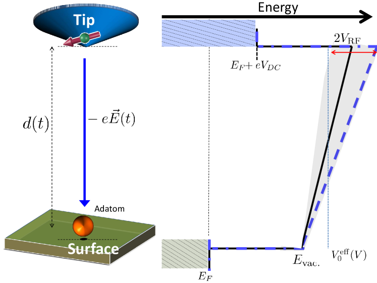
A quite accurate description of the transmission amplitude in an STM junction is given in terms of the Tersoff-Hamann model [68]. In this approach, the tip is modeled as a geometrical point, so that the tip effect can be simplified and factorized out of the problem, with the tunneling amplitude proportional to the surface wavefunction at the tip position and inversely proportional to the decay constant . An even simpler description of the STM junction can be provided by a one-dimensional square barrier at zero-bias voltage, assuming the same tip and surface work-functions, which evolves into a tilted barrier at finite bias voltage. Under this description, one can obtain a simple relation of the hybridization constants and the energy-dependent transmission amplitude. Strictly speaking, under a finite bias, we should solve the problem of a triangular barrier, which involves the Airy functions [69] and cumbersome expressions of the transmission amplitudes . This approach was used in Ref. ([32]) where it was shown that the transmission amplitude could be expressed as , where is the transmission amplitude in the absence of bias voltage.
| (27) |
where we have considered an opaque barrier and taken the values at the Fermi level, i.e., , with the effective mass and the tip-surface distance. This simple dependence is also reproduced in the Tersoff-Hamann model [70]. Here we should make the following remark. This result is based on the assumption that the effective barrier height changes linearly with the applied bias voltage , i.e., . The coefficient will depend on the electrostatic characteristics of the tip-sample junction. In the above results, we have assumed that the drop in the potential induced by the bias voltage occurs at the tip, while the surface’s chemical potential is unaffected by the bias voltage. This asymmetric situation is common in STM junctions, while for quantum dots coupled to similar electrodes, the drop would occur symmetrically in the tip and surface chemical potentials, leading to . Given the highly nontrivial potential dependence found by DFT in the MgO/Ag(100) surface under a finite electric field [67], an accurate description of the effect of the electric field on the transmission may require to use a numerical estimation of the transmission function for a given self-consistent potential .
In any case, the central result is that we can relate the hybridization constants and the applied RF bias voltage to write down
| (28) |
A formal solution to the transport problem in the presence of a driving field requires using the Floquet theory in combination with the Keldysh Green’s function [71]. However, a much simpler description can be used for weak coupling and weak driving regimes. Here the essential assumption is that the dissipative part of the time evolution of the density matrix, which is described by a Lindblad super-operator [46], is not affected by the driving field. This approach is exactly the same used for the derivation of the optical Bloch equation of Sec. 2.1. In that case, the system evolves under an effective time-dependent Hamiltonian
| (29) |
where we have defined
| (30) |
A direct comparison of Eqs. (1) and (29) allows us to identify the Rabi frequency extracted from the cotunneling model, as examined in detailed in Ref. ([32]). First, we assumed that transition frequency is the only one close to the driving frequency . Mathematically this can be expressed as follows. If is the lifetime of state , and , for any pair of states different from or , . Then, one directly obtains by direct inspection that , where we have defined the global phase of the interaction such that .
3.3.1 Relation with the Kondo exchange mechanism
As mentioned at the beginning of Sec. 3.3, the single-orbital Anderson model can be mapped into the Kondo exchange coupling using the Schrieffer and Wolf canonical transformation. This procedure becomes far from trivial in the case of a multiorbital model. Thus, here we take an alternative mapping where our main goal will be to extract the relation between the exchange coupling of a single impurity and the virtual transition operators . For this purpose, we omit the potential scattering term and write the Kondo coupling as , where is the spin density at the impurity site and corresponds to the exchange of an electron scattering from the to the electrodes. Thus, introducing the Pauli matrices , we can write
| (32) | |||||
| (33) |
where we have introduced the notation . Notice that only the first term contributes to the spin-flip processes. In particular, the term responsible of rising the spin of the local spin is given by
| (34) |
Now we try to evaluate the equivalent term in the cotunneling Hamiltonian (24). The cotunneling Hamiltonian can be written as555Since we are interested only in the spin-flip processes, we can omit the correction term in diagonal in the electrodes degrees of freedom.
| (35) |
Now we make the following approximation. Since the scattering is dominated by processes close to the Fermi surface, we approximate the virtual transition operators by their values at the Fermi level. This approximation is consistent with the expression of the Kondo exchange Hamiltonian , where we have neglected the variation of the exchange coupling with the wave vectors. Then, we split the cotunneling Hamiltonian into two contributions, a spin-conserving and the spin-flip term. The last one is given by (after using the explicit quantum numbers)
| (36) |
where we have omitted the wave-vector index to indicate the values evaluated at the Fermi surface. A direct comparison of (34) and the equivalent term in (36) allows us to identify the Kondo-exchange coupling. For that, we project over the states and of the local spin (QS) connected by the Kondo coupling (cotunneling Hamiltonian)
| (37) |
where . This expression permits us to extract the effective exchange coupling from the cotunneling Hamiltonian. The explicit expressions of the virtual transition operators can be found in Appendix A.
Notice that either a variation of the charging energies or a variation of the hybridization constants will automatically reflect into a variation of the exchange constants .
Now we come back to the general Kondo Hamiltonian where, in addition to the exchange coupling proportional to , we may have a direct scattering term
| (38) |
where we have defined . Here is the identity in the Hilbert space of the local spin, and . Following an analysis similar to the one used for the spin-flip terms, and taking special care to split the spin-independent scattering and the spin-elastic scattering, we can arrive to the expression (see Appendix B for details):
| (39) |
It is worth pointing out that the cotunneling description and the Kondo exchange model with the parameters extracted from Eqs. (37) and (39) are not fully equivalent. This can be easily checked by looking at the result for the case of a transition metal adatom with the configuration, the counterpart, presented in Appendix C. The first important difference with the single orbital Anderson model, which can be mapped to the Kondo exchange model, is that the coupling with the reservoirs can occur through different orbitals. While in the case of the coupling to the STM tip it may be a reasonable ansatz, this may not be the case for the substrate coupling. If the coupling to the reservoir occurs only through one orbital state, the can be written as
| (40) | |||||
| (41) |
where . This result is the same that in the single Anderson impurity model obtained through the Schrieffer and Wolff transformation. Then, a second and more subtle difference appears in the virtual transition operator . Contrary to the single orbital Anderson model, the lowest energy states of the configuration correspond to a spin triplet (), with where the two electrons are located on different orbitals with parallel spins. Crucially, these three triplet states , and do not contribute to the spin-flip terms, nor to the potential scattering between tip and surface. Thus, we will need the next excited state for the transport properties, which is a spin and orbital singlet state, . A direct inspection of the transition matrix elements of leads to the following result:
| (42) | |||||
| (43) |
These results are qualitatively analogous to those obtained for the single orbital Anderson model, see Eqs. (58) and (61) in Appendix C. Here we have neglected the denominator’s energy differences, considering that the typical addition and removal energies are of the order of 1 eV or larger. Moreover, we have neglected contributions from other virtual states, which can be of the order of a 10%.
Finally, these results deserve additional comments. First, the approximations involved in (42) do not hold in general. They are based on the assumption that tip and substrate couplings are only with the orbital of the transition metal atom. In addition, the specific properties , and , which leads to a negligible contribution of the (virtual) lowest energy triplet, are specific of the symmetry considered. Second, the cotunneling description includes effects that are not considered within the standard exchange coupling description, mainly the charge fluctuations. For instance, the spin Hamiltonian dressing due to a Kondo exchange coupling can only affect the spin spectrum when the reservoir is spin-polarized, playing the role of an effective magnetic field, as in Eq. (21). However, the cotunneling Hamiltonian includes a finite correction even for the coupling to a spin-averaging electrode. This has important consequences for the STM-ESR since, as described in Ref. ([32]), it can explain the DC current-independent Rabi frequency observed for some STM tips [12].
Recent calculations based on the cotunneling physics, computing the full time-dependent current through an atomic orbital in the presence of atomic magnetic transitions [72] shows that the modulation of the hopping amplitude in time, or equivalently, the modulation of the tunnel barrier by the driving electric field, is far enough to reproduce the STM-ESR spectra as a function of driving frequency. As in the above theory, the problem is the degree of actual change of the barrier by the driving field. Although in the simple description used in Eq. (27), we have assumed that the RF modulation only affects the barrier height, a more precise picture would also require to account for the barrier width variation associated with the piezoelectric displacement discussed in Sec. 3.1. Nevertheless, both effects will give place to a modulation of the hopping amplitudes , Eq. (26), as considered in the cotunneling picture. Our calculations seem to indicate that sizeable barrier modulations are achievable with usual STM-induced fields, leading us to the upbeat conclusion that STM-ESR should transcend the use of MgO as the sole STM-ESR substrate.
3.4 Other possible origins
In addition to the physical mechanisms signaled above, several alternative explanations deserve some comments. Although under the current experimental conditions of STM-ESR, the present experimental data suggest they may have a negligible contribution, they could be relevant under different experimental conditions. A novel mechanism was proposed by Shakirov et al. [33], who suggested that the resonance effect is a consequence of the spin-transfer-torque (STT), i.e., the nonlinearity of the coupling between the magnetic moment and the spin-polarized current. This nonlinear process is enhanced near resonance, and it is proportional to the square of the driving amplitude . Moreover, the effect does not rely on any mechanical or orbital degrees of freedom, involving only the dissipative interaction with the spin-polarized tunnel current, which agrees well with the observed ubiquity of the resonant effect.
When compared to the experimental findings, the peak resonance signal was found to be proportional to the DC current and to saturate with the RF bias voltage [12], in contrast to the quadratic dependence expected from the STT mechanism. Moreover, the strong dependence of the Rabi frequency with the standpoint distance at constant DC setpoint current does not seem compatible with this mechanism [20].
The modulation of the tunnel barrier by the exchange interaction between the localized spin and the tunneling electrons was already suggested [73, 6] as a possible origin of the resonance signal after the first STM-ESR attempts. Although this mechanism can be related to the exchange mechanism of Sec.3.1.1 and the cotunneling mechanism of Sec. 3.3, the theoretical treatment was based on the analysis of the elastic current. It was argued that the barrier height for a particular electron scattering has a contribution coming from magnetic coupling, which depends on the average spin. This gives place to a modulation of the current that depends on the relative orientation between the localized spin and the tunneling electron’s spin. Then, they adduced that tunneling electrons keep the memory of the spin polarization on a finite time scale, leading to a nonzero instantaneous spin current that could be related to the 1/ noise features [73].
The modulation of the tunnel barrier is also behind a class of proposed physical mechanisms where the relativistic effects are essential for magnetic resonance. Balatsky et al. proposed a mechanism where the modulation of the tunnel barrier was mediated by the spin-orbit interaction of the substrate-metal conduction electrons [74]. This effect translates into a current-independent modulation of the density of states by the precessing spin, which should work even in the absence of current spin-polarization, in contrast with the broadly accepted STM-ESR measurements [9, 10, 11, 12, 13, 14, 15, 16, 17, 18, 19, 20, 21, 22, 23]. The modulation of the tunneling barrier by the electric dipole moment originating from the spin-orbit interaction was also considered by Shachal and Manassen [75], but this effect was later estimated to be negligible [76]. Other mechanisms mediated by relativistic effects were the coherent interference of the two resonance tunneling-current components passing through the Zeeman levels split by the static magnetic field [77], spin-flip coupling between the conduction electrons on the localized spin site and electrodes [78], coherent tunneling of a pair of electrons with opposite spins [79] among others [6].
4 Concluding remarks
The growing number of experimental results on STM-ESR is starting to delineate the role of the different experimental variables that control the resonance signal. They have clarified the relevance of the DC and RF bias voltage, the tunnel conductance, the temperature, or some of the tip microscopic details [12, 20, 21].
A clear picture emerges where the coupling with the spin-polarized tip plays a key role. STM-ESR can be observed even in the absence of external static magnetic field [16, 22], but the tip polarization is indispensable. Once the magnetic field associated with the RF electric field has been discarded due to its tiny magnitude [18, 25], the tip-induced magnetic field appears as the most likely source of coupling between the RF electric field and the local spin. The data point at two sources of tip-induced magnetic field [20], a dipolar one due to the direct interaction between the dipolar moment of the adatom and of the magnetic tip, and an exchange-field one that is shorter range. The exchange field has been argued to be sufficient to explain STM-ESR on Fe adatoms [30], but recent data suggest that the longer-range contribution of the dipolar field is needed [20]. The exchange field source is ultimately the Kondo exchange that is due to the overlap of the tip and adatom electronic wave function. As such, the tunneling barrier between tip and adatom becomes a fundamental ingredient to induce sizeable exchange fields.
There is s growing consensus on the need to have a tip-induced magnetic field, as we just saw, but one mandatory ingredient is needed; a time-dependent field. Indeed, ESR requires an RF oscillating magnetic field acting on the magnetic adatom. Several related mechanisms could explain this oscillating field. On one side, different works point to the piezoelectric displacement of the adatom with the RF electric field. Estimations based on density functional calculations combined with multiplet calculations shows in general qualitative agreement with the experimentally observed Rabi frequency [30, 18, 20]. The differences, which can vary from a factor 2-4 [20, 30] to almost a factor 40 [18], have been attributed to the harmonic approximation in the estimation of the recovery constant [20] or to the piezoelectric motion of the MgO layer, as well as the motion of the Fe atom at the tip apex [18]. Independent of the other piezoelectric displacement sources, it is clear that this mechanism can drive an RF magnetic coupling with the local spin. However, the cotunneling proposal [32] shows that a piezoelectric response is not needed long as the RF electric field strongly modifies the tunneling probability for the electron. In this case, the tunneling barrier modulation leads to an effective time-dependent magnetic field that suffices to induce Rabi oscillations. The piezoelectric effect enhances the barrier modulation, facilitating the appearance of the magnetic resonance. For these reasons, we believe that STM-ESR should be feasible on different types of substrates other than MgO/Ag(100).
Acknowledgements
We are pleased to thank our collaborators for important discussions. A non-exhaustive list of the many contributors to our discussions is: D.-J. Choi, T. Choi, F. Donatti, A. J. Heinrich, J. Fernández-Rossier, P. Gambardella, L. Limot, F. Natterer, J. Reina Gálvez, T. Seifert, S. Stepanow, P. Willke, C. Wolf. Financial support from the Spanish MICINN (projects RTI2018-097895-B-C44, PlD2019-109539G8-C41, ) is gratefully acknowledged. FD acknowledges financial support from Basque Government, grant IT986-16 and Canary Islands program Viera y Clavijo (Ref. 2017/0000231).
Appendix A Virtual transition operators for the cotunneling model
In the case of a multiorbital correlated QS weakly coupled to the electrodes, the matrix elements of the virtual transition operators between the eigenstates of are given by [65, 32]:
| (44) |
where labels the eigenstates of with electrons, is the ground state energy of , denotes the quasiparticle energy, and and .666For clarity reasons, here we have assumed real coupling matrix elements Here and denotes the annihilation and creation operators in the orbital of the QS with spin .
Appendix B Derivation of the direct scattering term
In the case of the elastic scattering, we need to include not only the off-diagonal terms of the cotunneling Hamiltonian but also the diagonal ones. This makes it necessary to include the corrected cotunneling Hamiltonian instead of since the diagonal terms will also contribute to the spin-conserving processes. First, we project on the states , where denotes an eigenstate of the reservoir with spin and energy
For the cotunneling Hamiltonian , the matrix elements will be given by
| (48) | |||||
As we did for the spin-flip terms, we consider that the scattering processes are mainly due to the vicinity of the Fermi surface and, besides, we also assume that the hoppings do not depend on the direction of the wave-vector . Moreover, we particularize the previous expressions for the case and , so that
| (51) | |||||
We now evaluate the spin-conserving terms of . As for the cotunneling Hamiltonian, we look at the matrix elements of the Kondo Hamiltonian and the states . Then, we get
| (53) | |||||
where we have introduced the short notation . A direct comparison between expressions (53) and (51) allows us to identify the following relation:
| (54) |
which is the equation used in the main text.
Appendix C Example of an electronic configuration: the TiH on MgO (bridge position)
We now calculate the transition matrix elements obtained from the multiplet calculation for the TiH adatom on the bridge side of MgO/Ag(100). In that system, the lowest energy orbital state corresponds to the orbital (). We thus assume that only this orbital is hybridized with the surface and tip electrodes, with intensities and , respectively (we assume that those couplings are real). In addition, we evaluate the different operators only at the Fermi level, i.e., .
We first start calculating the expressions of the operator and we particularize to the tip-substrate tunneling term. For clarity, we omit the electrode indexes whenever possible. Considering that the vacuum state has only one state, , we have that
| (55) |
where we have defined . Notice that, since the orbital state is the (non-degenerate) ground state in the presence of the crystal field can be written as , where the label denotes the orbital state. Hence, we have for the spin-flip terms the following operators in the bases:
| (58) |
and the spin conserving term
| (61) |
(Similarly for the matrix elements).
We now consider the operator. In the first place, we remind the results obtained for the single Anderson impurity model. In that case, the charged state with two electrons consists of a doubly occupied singlet state . Then, one gets the following transition operators
| (64) |
and the spin conserving term
| (67) |
where , with . Let us come back to the TiH system. Neglecting the energy differences in the denominator, and contributions from other higher energy states, which could account for corrections of the order of 10%, we get that
| (70) |
For the spin-conserving terms, we find that
| (73) |
With this expressions we can arrive to the following relations:
| (74) |
and
| (75) |
If we particularize to the case of electron-hole symmetry, where , and considering that and , as it corresponds to an isotropic spin system in a field , we get that
| (76) |
and
| (77) |
These last two equations correspond to the Schrieffer and Wolff transformation results for the spin system [63].
References
- [1] A. Abragam, B. Bleaney, Electron Paramagnetic Resonance of Transition Ions, Oxford University Press, Oxford, 1970.
-
[2]
R. M. Fratila, A. H. Velders,
Small-volume
nuclear magnetic resonance spectroscopy, Annual Review of Analytical
Chemistry 4 (1) (2011) 227–249.
doi:10.1146/annurev-anchem-061010-114024.
URL https://doi.org/10.1146/annurev-anchem-061010-114024 -
[3]
H. J. Mamin, M. Kim, M. H. Sherwood, C. T. Rettner, K. Ohno, D. D. Awschalom,
D. Rugar,
Nanoscale nuclear
magnetic resonance with a nitrogen-vacancy spin sensor, Science 339 (6119)
(2013) 557–560.
arXiv:https://science.sciencemag.org/content/339/6119/557.full.pdf,
doi:10.1126/science.1231540.
URL https://science.sciencemag.org/content/339/6119/557 - [4] D. R. Glenn, D. B. Bucher, J. Lee, M. D. Lukin, H. Park, R. L. Walsworth, High-resolution magnetic resonance spectroscopy using a solid-state spin sensor, Nature 555 (7696) (2018) 351–354.
-
[5]
Y. Manassen, R. J. Hamers, J. E. Demuth, A. J. Castellano Jr.,
Direct
observation of the precession of individual paramagnetic spins on oxidized
silicon surfaces, Phys. Rev. Lett. 62 (1989) 2531–2534.
doi:10.1103/PhysRevLett.62.2531.
URL https://link.aps.org/doi/10.1103/PhysRevLett.62.2531 -
[6]
A. V. Balatsky, M. Nishijima, Y. Manassen,
Electron spin
resonance-scanning tunneling microscopy, Advances in Physics 61 (2) (2012)
117–152.
doi:10.1080/00018732.2012.668775.
URL https://doi.org/10.1080/00018732.2012.668775 -
[7]
S. Müllegger, S. Tebi, A. K. Das, W. Schöfberger, F. Faschinger, R. Koch,
Radio
frequency scanning tunneling spectroscopy for single-molecule spin
resonance, Phys. Rev. Lett. 113 (2014) 133001.
doi:10.1103/PhysRevLett.113.133001.
URL https://link.aps.org/doi/10.1103/PhysRevLett.113.133001 -
[8]
S. Müllegger, E. Rauls, U. Gerstmann, S. Tebi, G. Serrano,
S. Wiespointner-Baumgarthuber, W. G. Schmidt, R. Koch,
Mechanism for
nuclear and electron spin excitation by radio frequency current, Phys. Rev.
B 92 (2015) 220418.
doi:10.1103/PhysRevB.92.220418.
URL https://link.aps.org/doi/10.1103/PhysRevB.92.220418 - [9] S. Baumann, W. Paul, T. Choi, C. P. Lutz, A. Ardavan, A. J. Heinrich, Electron paramagnetic resonance of individual atoms on a surface, Science 350 (6259) (2015) 417–420. doi:10.1126/science.aac8703.
- [10] F. D. Natterer, K. Yang, W. Paul, P. Willke, T. Choi, T. Greber, A. J. Heinrich, C. P. Lutz, Reading and writing single-atom magnets, Nature 543 (7644) (2017) 226–228.
- [11] T. Choi, W. Paul, S. Rolf-Pissarczyk, A. J. Macdonald, F. D. Natterer, K. Yang, P. Willke, C. P. Lutz, A. J. Heinrich, Atomic-scale sensing of the magnetic dipolar field from single atoms, Nature nanotechnology 12 (5) (2017) 420.
- [12] P. Willke, W. Paul, F. D. Natterer, K. Yang, Y. Bae, T. Choi, J. Fernández-Rossier, A. J. Heinrich, C. P. Lutz, Probing quantum coherence in single-atom electron spin resonance, Science Advances 4 (2). arXiv:http://advances.sciencemag.org/content/4/2/eaaq1543.full.pdf, doi:10.1126/sciadv.aaq1543.
-
[13]
K. Yang, Y. Bae, W. Paul, F. D. Natterer, P. Willke, J. L. Lado, A. Ferrón,
T. Choi, J. Fernández-Rossier, A. J. Heinrich, C. P. Lutz,
Engineering
the eigenstates of coupled spin- atoms on a surface, Phys. Rev. Lett.
119 (2017) 227206.
doi:10.1103/PhysRevLett.119.227206.
URL https://link.aps.org/doi/10.1103/PhysRevLett.119.227206 -
[14]
P. Willke, Y. Bae, K. Yang, J. L. Lado, A. Ferrón, T. Choi, A. Ardavan,
J. Fernández-Rossier, A. J. Heinrich, C. P. Lutz,
Hyperfine
interaction of individual atoms on a surface, Science 362 (6412) (2018)
336–339.
arXiv:http://science.sciencemag.org/content/362/6412/336.full.pdf,
doi:10.1126/science.aat7047.
URL http://science.sciencemag.org/content/362/6412/336 -
[15]
Y. Bae, K. Yang, P. Willke, T. Choi, A. J. Heinrich, C. P. Lutz,
Enhanced quantum
coherence in exchange coupled spins via singlet-triplet transitions, Science
Advances 4 (11).
arXiv:https://advances.sciencemag.org/content/4/11/eaau4159.full.pdf,
doi:10.1126/sciadv.aau4159.
URL https://advances.sciencemag.org/content/4/11/eaau4159 -
[16]
P. Willke, A. Singha, X. Zhang, T. Esat, C. P. Lutz, A. J. Heinrich, T. Choi,
Tuning single-atom
electron spin resonance in a vector magnetic field, Nano Letters 19 (11)
(2019) 8201–8206, pMID: 31661282.
doi:10.1021/acs.nanolett.9b03559.
URL https://doi.org/10.1021/acs.nanolett.9b03559 - [17] P. Willke, K. Yang, Y. Bae, A. J. Heinrich, C. P. Lutz, Magnetic resonance imaging of single atoms on a surface, Nature Physics 15 (10) (2019) 1005–1010.
-
[18]
K. Yang, W. Paul, F. D. Natterer, J. L. Lado, Y. Bae, P. Willke, T. Choi,
A. Ferrón, J. Fernández-Rossier, A. J. Heinrich, C. P. Lutz,
Tuning the
exchange bias on a single atom from 1 mt to 10 t, Phys. Rev. Lett. 122
(2019) 227203.
doi:10.1103/PhysRevLett.122.227203.
URL https://link.aps.org/doi/10.1103/PhysRevLett.122.227203 -
[19]
K. Yang, W. Paul, S.-H. Phark, P. Willke, Y. Bae, T. Choi, T. Esat, A. Ardavan,
A. J. Heinrich, C. P. Lutz,
Coherent spin
manipulation of individual atoms on a surface, Science 366 (6464) (2019)
509–512.
arXiv:https://science.sciencemag.org/content/366/6464/509.full.pdf,
doi:10.1126/science.aay6779.
URL https://science.sciencemag.org/content/366/6464/509 -
[20]
T. S. Seifert, S. Kovarik, D. M. Juraschek, N. A. Spaldin, P. Gambardella,
S. Stepanow,
Longitudinal and
transverse electron paramagnetic resonance in a scanning tunneling
microscope, Science Advances 6 (40).
arXiv:https://advances.sciencemag.org/content/6/40/eabc5511.full.pdf,
doi:10.1126/sciadv.abc5511.
URL https://advances.sciencemag.org/content/6/40/eabc5511 - [21] W. M. van Weerdenburg, M. Steinbrecher, N. P. van Mullekom, J. W. Gerritsen, H. von Allwörden, F. D. Natterer, A. A. Khajetoorians, A scanning tunneling microscope capable of electron spin resonance and pump-probe spectroscopy at mk temperature and in vector magnetic field, arXiv preprint arXiv:2007.01835.
- [22] M. Steinbrecher, W. M. van Weerdenburg, E. F. Walraven, N. P. van Mullekom, J. W. Gerritsen, F. D. Natterer, D. I. Badrtdinov, A. N. Rudenko, V. V. Mazurenko, M. I. Katsnelson, et al., Quantifying the interplay between fine structure and geometry of an individual molecule on a surface, arXiv preprint arXiv:2007.01928.
- [23] L. M. Veldman, L. Farinacci, R. Rejali, R. Broekhoven, J. Gobeil, D. Coffey, M. Ternes, A. F. Otte, Free coherent evolution of a coupled atomic spin system initialized by electron scattering (2021).
- [24] K. Yang, P. Willke, Y. Bae, A. Ferrón, J. L. Lado, A. Ardavan, J. Fernández-Rossier, A. J. Heinrich, C. P. Lutz, Electrically controlled nuclear polarization of individual atoms, Nature nanotechnology 13 (12) (2018) 1120.
-
[25]
T. S. Seifert, S. Kovarik, C. Nistor, L. Persichetti, S. Stepanow,
P. Gambardella,
Single-atom
electron paramagnetic resonance in a scanning tunneling microscope driven by
a radio-frequency antenna at 4 k, Phys. Rev. Research 2 (2020) 013032.
doi:10.1103/PhysRevResearch.2.013032.
URL https://link.aps.org/doi/10.1103/PhysRevResearch.2.013032 -
[26]
M. Atatüre, J. Dreiser, A. Badolato, A. Högele, K. Karrai, A. Imamoglu,
Quantum-Dot
Spin-State Preparation with Near-Unity Fidelity, Science
312 (5773) (2006) 551–553, publisher: American Association for the
Advancement of Science Section: Report.
doi:10.1126/science.1126074.
URL http://science.sciencemag.org/content/312/5773/551 -
[27]
D. Press, T. D. Ladd, B. Zhang, Y. Yamamoto,
Complete quantum control of
a single quantum dot spin using ultrafast optical pulses, Nature 456 (7219)
(2008) 218–221, number: 7219 Publisher: Nature Publishing Group.
doi:10.1038/nature07530.
URL http://www.nature.com/articles/nature07530 -
[28]
S. L. Bayliss, D. W. Laorenza, P. J. Mintun, B. D. Kovos, D. E. Freedman, D. D.
Awschalom,
Optically
addressable molecular spins for quantum information processing, Science
370 (6522) (2020) 1309–1312, publisher: American Association for the
Advancement of Science Section: Report.
doi:10.1126/science.abb9352.
URL http://science.sciencemag.org/content/370/6522/1309 - [29] P. Berggren, J. Fransson, Electron paramagnetic resonance of single magnetic moment on a surface, Scientific reports 6 (2016) 25584.
-
[30]
J. L. Lado, A. Ferrón, J. Fernández-Rossier,
Exchange mechanism
for electron paramagnetic resonance of individual adatoms, Phys. Rev. B 96
(2017) 205420.
doi:10.1103/PhysRevB.96.205420.
URL https://link.aps.org/doi/10.1103/PhysRevB.96.205420 -
[31]
A. Ferrón, S. A. Rodríguez, S. S. Gómez, J. L. Lado,
J. Fernández-Rossier,
Single spin
resonance driven by electric modulation of the -factor anisotropy, Phys.
Rev. Research 1 (2019) 033185.
doi:10.1103/PhysRevResearch.1.033185.
URL https://link.aps.org/doi/10.1103/PhysRevResearch.1.033185 -
[32]
J. Reina Gálvez, C. Wolf, F. Delgado, N. Lorente,
Cotunneling
mechanism for all-electrical electron spin resonance of single adsorbed
atoms, Phys. Rev. B 100 (2019) 035411.
doi:10.1103/PhysRevB.100.035411.
URL https://link.aps.org/doi/10.1103/PhysRevB.100.035411 - [33] A. M. Shakirov, A. N. Rubtsov, P. Ribeiro, Spin transfer torque induced paramagnetic resonance, Phys. Rev. B 99 (2019) 054434. doi:10.1103/PhysRevB.99.054434.
-
[34]
W. E. Moerner, L. Kador,
Optical detection
and spectroscopy of single molecules in a solid, Phys. Rev. Lett. 62 (1989)
2535–2538.
doi:10.1103/PhysRevLett.62.2535.
URL https://link.aps.org/doi/10.1103/PhysRevLett.62.2535 -
[35]
G. M. Steeves, A. Y. Elezzabi, M. R. Freeman,
Nanometer-scale imaging with an
ultrafast scanning tunneling microscope, Applied Physics Letters 72 (4)
(1998) 504–506.
arXiv:https://doi.org/10.1063/1.120798, doi:10.1063/1.120798.
URL https://doi.org/10.1063/1.120798 - [36] S. Yampolsky, D. A. Fishman, S. Dey, E. Hulkko, M. Banik, E. O. Potma, V. A. Apkarian, Seeing a single molecule vibrate through time-resolved coherent anti-stokes raman scattering, Nature Photonics 8 (8) (2014) 650–656.
-
[37]
M. Orrit, J. Bernard,
Single pentacene
molecules detected by fluorescence excitation in a p-terphenyl crystal,
Phys. Rev. Lett. 65 (1990) 2716–2719.
doi:10.1103/PhysRevLett.65.2716.
URL https://link.aps.org/doi/10.1103/PhysRevLett.65.2716 -
[38]
T. Plakhotnik, D. Walser, M. Pirotta, A. Renn, U. P. Wild,
Nonlinear
spectroscopy on a single quantum system: Two-photon absorption of a single
molecule, Science 271 (5256) (1996) 1703–1705.
arXiv:https://science.sciencemag.org/content/271/5256/1703.full.pdf,
doi:10.1126/science.271.5256.1703.
URL https://science.sciencemag.org/content/271/5256/1703 -
[39]
A. Gaiduk, M. Yorulmaz, P. V. Ruijgrok, M. Orrit,
Room-temperature
detection of a single molecule’s absorption by photothermal
contrast, Science 330 (6002) (2010) 353–356.
arXiv:https://science.sciencemag.org/content/330/6002/353.full.pdf,
doi:10.1126/science.1195475.
URL https://science.sciencemag.org/content/330/6002/353 - [40] M. Reutzel, A. Li, Z. Wang, H. Petek, Coherent multidimensional photoelectron spectroscopy of ultrafast quasiparticle dressing by light, Nature communications 11 (1) (2020) 1–5.
-
[41]
D. A. Yarotski, R. D. Averitt, N. Negre, S. A. Crooker, A. J. Taylor, G. P.
Donati, A. Stintz, L. F. Lester, K. J. Malloy,
Ultrafast
carrier-relaxation dynamics in self-assembled inas/gaas quantum dots, J.
Opt. Soc. Am. B 19 (6) (2002) 1480–1484.
doi:10.1364/JOSAB.19.001480.
URL http://josab.osa.org/abstract.cfm?URI=josab-19-6-1480 - [42] Y. Terada, S. Yoshida, O. Takeuchi, H. Shigekawa, Real-space imaging of transient carrier dynamics by nanoscale pump–probe microscopy, Nature photonics 4 (12) (2010) 869.
- [43] T. L. Cocker, V. Jelic, M. Gupta, S. J. Molesky, J. A. Burgess, G. De Los Reyes, L. V. Titova, Y. Y. Tsui, M. R. Freeman, F. A. Hegmann, An ultrafast terahertz scanning tunnelling microscope, Nature Photonics 7 (8) (2013) 620–625.
- [44] T. L. Cocker, D. Peller, P. Yu, J. Repp, R. Huber, Tracking the ultrafast motion of a single molecule by femtosecond orbital imaging, Nature 539 (7628) (2016) 263–267.
- [45] C. Cohen-Tannoudji, G. Grynberg, J. Dupont-Roc, Atom-Photon Interactions, Wiley and Sons, INC., New York, 1998.
- [46] H.-P. Breuer, F. Petruccione, The theory of open quantum systems, Oxford University Press, 2002.
- [47] K. Yosida, Theory of Magnetism (Springer Series in Solid-State Sciences), Springer, 2001.
-
[48]
J.-P. Gauyacq, N. Lorente,
Decoherence-governed
magnetic-moment dynamics of supported atomic objects, Journal of Physics:
Condensed Matter 27 (45) (2015) 455301.
doi:10.1088/0953-8984/27/45/455301.
URL http://stacks.iop.org/0953-8984/27/i=45/a=455301 - [49] F. Delgado, J. Fernández-Rossier, Storage of classical information in quantum spins, Phys. Rev. Lett. 108 (2012) 196602. doi:10.1103/PhysRevLett.108.196602.
- [50] F. Delgado, J. Fernández-Rossier, Spin decoherence of magnetic atoms on surfaces, Progress in Surface Science 92 (1) (2017) 40–82.
- [51] F. Delgado, J. Fernández-Rossier, Spin dynamics of current-driven single magnetic adatoms and molecules, Phys. Rev. B 82 (13) (2010) 134414. doi:10.1103/PhysRevB.82.134414.
-
[52]
G. Shavit, B. Horovitz, M. Goldstein,
Generalized open
quantum system approach for the electron paramagnetic resonance of magnetic
atoms, Phys. Rev. B 99 (2019) 195433.
doi:10.1103/PhysRevB.99.195433.
URL https://link.aps.org/doi/10.1103/PhysRevB.99.195433 - [53] J. Korringa, Nuclear magnetic relaxation and resonnance line shift in metals, Physica 16 (7) (1950) 601–610.
- [54] S. Yan, D.-J. Choi, J. A. Burgess, S. Rolf-Pissarczyk, S. Loth, Control of quantum magnets by atomic exchange bias, Nature nanotechnology 10 (1) (2015) 40.
- [55] R. Rejali, D. Coffey, J. Gobeil, J. W. González, F. Delgado, A. F. Otte, Complete reversal of the atomic unquenched orbital moment by a single electron, npj Quantum Materials 5 (1) (2020) 1–7.
-
[56]
E. M. Chudnovsky, D. A. Garanin, R. Schilling,
Universal
mechanism of spin relaxation in solids, Phys. Rev. B 72 (2005) 094426.
doi:10.1103/PhysRevB.72.094426.
URL https://link.aps.org/doi/10.1103/PhysRevB.72.094426 -
[57]
C. Calero, E. M. Chudnovsky,
Rabi Spin
Oscillations Generated by Ultrasound in Solids, Physical Review
Letters 99 (4).
doi:10.1103/PhysRevLett.99.047201.
URL https://link.aps.org/doi/10.1103/PhysRevLett.99.047201 -
[58]
P. W. Anderson,
Localized magnetic
states in metals, Phys. Rev. 124 (1961) 41–53.
doi:10.1103/PhysRev.124.41.
URL https://link.aps.org/doi/10.1103/PhysRev.124.41 - [59] J. Kondo, Resistance minimum in dilute magnetic alloys, Prog. Theor. Phys. 32 (1964) 37–49.
- [60] M. Ternes, Probing magnetic excitations and correlations in single and coupled spin systems with scanning tunneling spectroscopy, Progress in Surface Science 92 (1) (2017) 83 – 115.
-
[61]
D.-J. Choi, N. Lorente, J. Wiebe, K. von Bergmann, A. F. Otte, A. J. Heinrich,
Colloquium:
Atomic spin chains on surfaces, Rev. Mod. Phys. 91 (2019) 041001.
doi:10.1103/RevModPhys.91.041001.
URL https://link.aps.org/doi/10.1103/RevModPhys.91.041001 - [62] A. Khajetoorians, M. Valentyuk, M. Steinbrecher, T. Schlenk, A. Shick, J. Kolorenc, A. Lichtenstein, T. Wehling, R. Wiesendanger, J. Wiebe, Tuning emergent magnetism in a hund’s impurity, Nature nanotechnology 10 (11) (2015) 958–964.
- [63] J. R. Schrieffer, P. A. Wolff, Relation between the Anderson and Kondo Hamiltonians, Phys. Rev. 149 (1966) 491–492.
- [64] M. Ternes, Spin excitations and correlations in scanning tunneling spectroscopy, New Journal of Physics 17 (6) (2015) 063016.
- [65] F. Delgado, J. Fernández-Rossier, Cotunneling theory of atomic spin inelastic electron tunneling spectroscopy, Phys. Rev. B 84 (2011) 045439. doi:10.1103/PhysRevB.84.045439.
- [66] A. P. Jauho, N. S. Wingreen, Y. Meir, Time-dependent transport in interacting an noninteracting resonant-tunneling systems, Phys. Rev. B. 50 (1994) 5528.
- [67] C. Wolf, F. Delgado, J. Reina, N. Lorente, Efficient ab initio multiplet calculations for magnetic adatoms on mgo, The Journal of Physical Chemistry A 124 (11) (2020) 2318–2327.
- [68] J. Tersoff, D. R. Hamann, Theory of the scanning tunneling microscope, Phys. Rev. B 31 (1985) 805–813. doi:10.1103/PhysRevB.31.805.
- [69] R. H. Fowler, L. Nordheim, Electron emission in intense electric fields, Proc. R. Soc. Lond. 119 (781) (1928) 173–181.
- [70] S. Lounis, Theory of scanning tunneling microscopy, ArXiv:1404.0961.
-
[71]
B. Baran, T. Domański,
Quasiparticles of
a periodically driven quantum dot coupled between superconducting and normal
leads, Phys. Rev. B 100 (2019) 085414.
doi:10.1103/PhysRevB.100.085414.
URL https://link.aps.org/doi/10.1103/PhysRevB.100.085414 - [72] José Reina et al., unpublished.
-
[73]
Y. Manassen, A. V. Balatsky,
1/f
spin noise and a single spin detection with stm, Israel Journal of Chemistry
44 (4) (2004) 401–408.
arXiv:https://onlinelibrary.wiley.com/doi/pdf/10.1560/QD9U-ULHL-6NWH-V0U0,
doi:https://doi.org/10.1560/QD9U-ULHL-6NWH-V0U0.
URL https://onlinelibrary.wiley.com/doi/abs/10.1560/QD9U-ULHL-6NWH-V0U0 - [74] A. Balatsky, I. Martin, Theory of single spin detection with stm, Quantum Information Processing 1 (5) (2002) 355–364.
-
[75]
D. Shachal, Y. Manassen,
Mechanism of
electron-spin resonance studied with use of scanning tunneling microscopy,
Phys. Rev. B 46 (1992) 4795–4805.
doi:10.1103/PhysRevB.46.4795.
URL https://link.aps.org/doi/10.1103/PhysRevB.46.4795 -
[76]
R. Prioli, J. S. Helman,
Effect of resonating
paramagnetic centers on the current of the scanning tunneling microscope,
Phys. Rev. B 52 (1995) 7887–7889.
doi:10.1103/PhysRevB.52.7887.
URL https://link.aps.org/doi/10.1103/PhysRevB.52.7887 -
[77]
D. Mozyrsky, L. Fedichkin, S. A. Gurvitz, G. P. Berman,
Interference
effects in resonant magnetotransport, Phys. Rev. B 66 (2002) 161313.
doi:10.1103/PhysRevB.66.161313.
URL https://link.aps.org/doi/10.1103/PhysRevB.66.161313 -
[78]
J.-X. Zhu, A. V. Balatsky,
Quantum
electronic transport through a precessing spin, Phys. Rev. Lett. 89 (2002)
286802.
doi:10.1103/PhysRevLett.89.286802.
URL https://link.aps.org/doi/10.1103/PhysRevLett.89.286802 -
[79]
S. Molotkov,
Theory
of electron-spin resonance topography of surfaces by the scanning tunneling
microscope, Surface Science 302 (1) (1994) 235 – 240.
doi:https://doi.org/10.1016/0039-6028(94)91113-4.
URL http://www.sciencedirect.com/science/article/pii/0039602894911134