A microfluidic method for passive trapping of sperms in microstructures

Abstract

Sperm motility is a prerequisite for male fertility. Enhancing the concentration of motile sperms in assisted reproductive technologies - for human and animal reproduction - is typically achieved through aggressive methods such as centrifugation. Here we propose a passive technique for the amplification of motile sperm concentration, with no externally imposed forces or flows. The technique is based upon the disparity between probability rates, for motile cells, of entering in and escaping from complex structures. The effectiveness of the technique is demonstrated in microfluidic experiments with microstructured devices, comparing the trapping power in different geometries. In these micro-traps we observe an enhancement of cells’ concentration close to $10$, with a contrast between motile and non-motile increased by a similar factor. Simulations of suitable interacting model sperms in realistic geometries reproduce quantitatively the experimental results, extend the range of observations and highlight the ingredients that are key to optimal trap design.

I Introduction

It is estimated that the male factor is the origin of roughly half of the case of fertility problems Barratt et al. (2009); Frey (2010). Improving the selection of motile sperms, particularly when they are rare, would be beneficial for assisted reproduction technologies, for both zootechnics and human reproduction. These aspects emphasize the importance of scientific research on sperm motility, particularly for mammals, a field which is certainly blessed by the recent advancements in imaging techniques, molecular biology and computational analysis Friedrich and Jülicher (2007); Friedrich et al. (2010); Gaffney et al. (2011); Guasto et al. (2020).

The most successful in-vitro fertilisation techniques (e.g. Fertilisation in Vitro and Embryo Transfer (FIVET) and Intracytoplasmic Sperm Injection (ICSI)) are highly aggressive, particularly for the female partner, and very expensive so that a part of the population cannot access them Schill et al. (2010). Less expensive techniques, such as Intrauterine Insemination (IUI), is even more dependent upon the selection of highly motile sperms, a problem which is typically solved by centrifuge, density gradients and swim-up techniques Boomsma et al. (2004) which can compromise the integrity of cells, mechanically or by exposition to DNA-disrupting chemical species Zini et al. (2000); Rappa et al. (2016). Sperm selection is also important for sperm cryopreservation. Established selection techniques are moreover poorly effective in the most serious cases of oligospermia ($<4$ million/ml) Smith and Takayama (2017). Microfluidics is certainly a promising road for the future of in-vitro fertilization Han et al. (2010); Matsuura et al. (2013); Chen et al. (2013); Tasoglu et al. (2013); Huang et al. (2015); Knowlton et al. (2015); Hussain et al. (2016); Zaferani et al. (2019). Microfluidic methods for sperm selection have been recently implemented Cho et al. (2003); Schuster et al. (2003), demonstrating interesting capabilities and important reduction of damaging probabilities Nosrati et al. (2014); Asghar et al. (2014); Rappa et al. (2016); Shirota et al. (2016); Xiao et al. (2021); Simchi et al. (2021). Many of these methods require the use of an external pumping in the micro-flows through channels, which is a further source of possible mechanical stress on the cells as well as a technological complication affecting costs. Microfluidics-based techniques for sperm sorting without external flow pumping have also been investigated recently Nosrati et al. (2014); Xiao et al. (2021); Simchi et al. (2021). In these studies the largest effort is devoted to the design of a ready-to-use chip for biomedical applications and to the evaluation of DNA fragmentation, while less attention is paid to the role of geometry and trap shapes, looking for possible physical effects that can enhance the sorting capacity.

The improvement of automatic techniques for separating motile cells from the non-motile ones can impact also diagnostic protocols. The evaluation of sperm concentration is typically operated by direct observation, under the optical microscope, in so-called Makler or Neubauer cameras, with noticeable approximation. The assessment of motility, not necessarily correlated with concentration, is another factor of subjectivity Agarwal et al. (2016) so that the classical male fertility exam, the spermiogram, is considered to be of not really high statistical significance Lu et al. (2010). Less subjective approaches include expensive systems such as CASA (Computer Assisted Sperm Analysis) and flow cytometry Graham (2001). Recent studies have evidenced how microfluidics is a promising technology for sperm diagnostics and point-of-care applications Zheng et al. (2011).

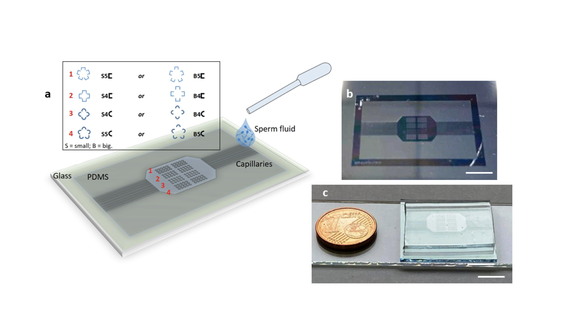
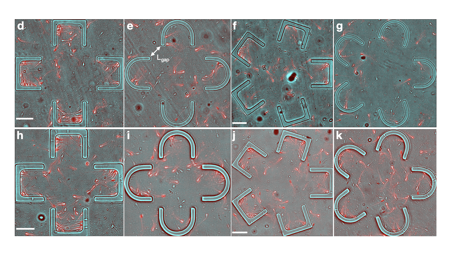
Figure 1: Design of microfluidic devices. a. Sketch of the quasi-2D hydrostastic microfluidic device showing the two networks of input /output capillaries connected to a cell sorter chamber including an array of microstructured trapping units. The chamber was filled, by capillarity, with bull sperm samples. The legend on the top shows geometric characteristics of the 4 groups of different shaped trapping units together with the corresponding acronyms used in the text. b. Picture of a patterned SU-8 master. c. Picture of the final microfluidic polydimethylsiloxane (PDMS) device for the passive trapping of sperms. Scale bars in b and c: $1cm$. (d-k): Microscope pictures with the design of the eight kinds of structures. The top row represents structures with big (B) gaps, $L_{gap}\approx 40\mu m$, the lower row structures with small (S) gaps, $L_{gap}\approx 20\mu m$. The pictures have been recorded in gray-scale from the microscope camera (see Methods) and coloured according to the following protocol. Red encodes motility, i.e. red level of each pixel indicates the variance of that pixel along a sequence of 7 frames centred around a given frame. The blue and green levels put in evidence structures and non-motile sperm cells, as they just encode the light level of the original central frame. Scale bars in d,f,h,j: $50\mu m$.

Our aim here is to demonstrate a new class of sperm sorting/concentration techniques which do not require external pumping in the micro-flows but still take advantage of low-cost and integrated microfluidic systems, obtained by soft-lithography microfabrication. This approach allows to enhance and modulate the confinement effects experienced by cells in their dynamics even in a restricted diffusion condition, typical of flow at the microscale. In this case, a pumped active flow is not really necessary, because the cells are motile by themselves and a separation can occur spontaneously. Indeed, non-motile (dead) sperms behave as passive particles dispersed in the fluid, and therefore diffuse very slowly without preferences for particular regions of the channel. The motile cells, as other kinds of cells equipped with self-propulsion (such as Escherichia coli, Bacillus subtilis and others) move very fast and display non-intuitive behavior in the presence of solid surfaces Elgeti et al. (2015); Nosrati et al. (2015); Rode et al. (2019), particularly adhesion Rothschild (1963); Li et al. (2008); Smith et al. (2009); Elgeti et al. (2010); Magdanz et al. (2015), swimming parallel to surfaces/obstacles Denissenko et al. (2012); Guidobaldi et al. (2014); Nosrati et al. (2015); Rode et al. (2019) but also long-time trapping in partially closed geometries Paoluzzi et al. (2020); Yaghoobi et al. (2021). The consequence of this behavior for filtering purposes on general models and on real bacteria have been studied theoretically and experimentally Galajda et al. (2007); Angelani et al. (2011); Koumakis et al. (2013, 2014). From the point of view of statistical physics, the demixing (e.g. separation between motile and non-motile cells) originates from the contrast between opposite thermodynamic situations, i.e. equilibrium (non-motile cells) vs. non-equilibrium (motile cells). In the first case, one cannot expect spontaneous de-mixing, as dictated by the second principle of thermodynamics, whereas in the latter case de-mixing is not forbidden, and the spontaneous ratchet effect due to asymmetric geometries is a way to realise it Makse et al. (1997); Di Leonardo et al. (2010); McCandlish et al. (2012); Gnoli et al. (2013); Medina-Sánchez et al. (2016); Chen et al. (2018); Striggow et al. (2020).

In our study we investigate experimentally a wide range of microstructures within an integrated microfluidic device to determine the key ingredients optimising the trapping/sorting power. A numerical simulation widen even more the range of accessible structures, confirming and deepening our understanding of the trapping mechanism. An important feature of sperm passive trapping, already emerged in previous research Guidobaldi et al. (2014), is the high trapping power of curved walls with small curvature radius, such as corners Nosrati et al. (2016). Inspired by those previous works, we take advantage of this effect to increase the sorting capability of a micro-structured fluidic device. Thanks to this observation, the maximum relative concentration (ratio between the density of motile cells inside and outside of the traps) achieved in our study doubles what found using geometries with large curvatures. We expect that our study can be a starting point for the development of point-of-care applications for male fertility diagnostics and for automatization of sperm sorting procedure finalised to the less expensive in vitro fertilization techniques (e.g. IUI).

II Results: experimental

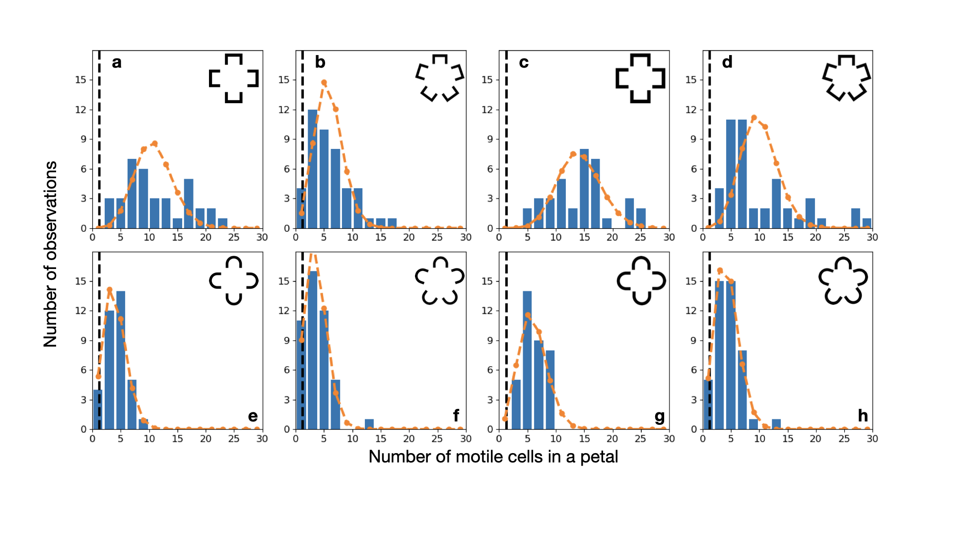
Figure 2: Concentration in petals (experiments). Histograms of the observed numbers of motile cells in each petals. Each bin has width $2$. The top four histograms are for the structures with $\sqsubset$-shaped petals, the lower fourhistograms are for the structures with $\subset$-shaped petals. The first two columns refer to big gap microstructures, $L_{gap}=40\mu m$, while the last two are small gap microstructures, $L_{gap}=20\mu m$. It is evident the larger trapping power of petals with $\sqsubset$-shape Poissonian distributions with the same average of the data are superimposed to the histograms in orange. Poissonian statistics is compatible with all data (p-value larger than $0.05$) apart from the first and last case of top row (B4$\sqsubset$ with $p=0.04$ and S5$\sqsubset$ with $p=10^{-5}$). The vertical dashed lines mark the number of motile cells that are found in the sperm liquid far from the structures, in an area equal to that of the petal.

Trapping experiments have been carried on using quasi-2D hydrostatic microfluidic devices. Each integrated device consists of two networks of input /output microchannels connected to the microstructured chamber (Fig. 1) and filled, by capillarity, with bull sperm samples after standard thawing protocols. The microfluidic trapping devices are realized in polydimethylsiloxane (PDMS) by conventional soft-lithography and replica-molding technique, starting from patterned SU-8 master ad hoc fabricated by photolithography Xia and Whitesides (1998). The chamber is designed as a functional cell sorter, with a total surface area of approximately $80\,mm^{2}$ and an internal volume of about $1.2\,\mu l$, and is micro-structured inside (Fig. 1a). A network of rectangular microfluidic-channels is used to allow the injection of the sample by capillary imbibition Viola et al. (2005) (see Methods for details). PDMS was chosen to ensure optical transparency for the real-time microscopy imaging, compatibility with cells and biomolecules, flexibility and high conformability with the master structure (Fig. 1b) Zizzari et al. (2019). The final sorting devices are produced by placing the microstructured polymeric replicas in conformal contact with glass substrates in order to obtain a perfect sealing of both microchannels and chamber. A picture of the final device is shown in Fig. 1c. The dimensions and characteristics of both the microfluidic chamber and of microstructures guarantee spontaneous imbibition and capillary displacement of the sample without any external pressure. In a microfluidic device with very low aspect ratio microstructures, the fluid displacement is in fact mainly driven by restricted diffusion and laminar flow Viola et al. (2005); Zizzari et al. (2014).

Details for microlithography and sample treatment procedures are given in the Methods. The design of the functional chambers is based upon an array with 4 groups of different shaped trapping units, each group contains several identical units separated by an average period of about $450\mu m$. Each trapping unit has a flower-like design made of n “petals” (with n = 4 or n = 5 and different shaped petals) around a central region: the spaces between petals are the inlets allowing sperm cells to enter or leave a trapping unit; in the following we call them “gaps”, their minimum distance is named $L_{gap}$ and in the two chamber designs it takes two values: $20\mu m$ (“S” small) and $40\mu m$ (“B” big). Each petal can have a “rounded” (  $\cap$  ) or “cornered” (  $\sqcap$  ) shape, see Fig. 1a. A given structure is denoted by the combination of the three possible parameters $L_{gap}\times n\times\textrm{shape}$, e.g. B4  $\cap$  stands for 4 rounded petals separated by big gaps, and this makes a total of 8 different kinds of traps, each repeated for at least 9 times in order to collect a larger statistics in the results. Several experiments in re-printed channels with the same design (together with cumulated observations at different times) allowed us to increase even further the statistics. The average area of a trapping structure is $\sim 225\,\mu m\times 225\,\mu m$ and the height of the channel is $\sim 15\mu m$, i.e. the trapping volume is - on average – $7\times 10^{-7}ml$. At the typical observed sample concentration $1.2-1.3\cdot 10^{7}$ motile cells per milliliter, one would find $\sim 8-9$ cells in a structure. On the contrary, the number of motile cells is found to be in the range of $20-80$, corresponding to a density enhancement of a factor $3-10$, depending upon the choice of $n$, $L_{gap}$ and the shape of the petals, as detailed in the rest of the work.

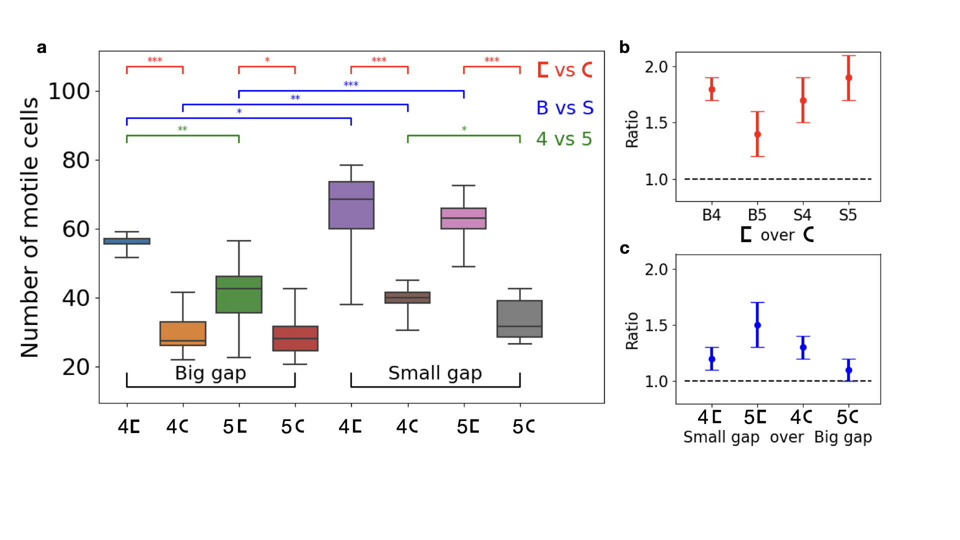
Figure 3: Concentration in structures (experiments). Total number of motile cells in each structure (experiments). a. Box-plot representing the distributions over several structures of the same kind: each colored box contains a line representing the median, its size covers the quartiles of the dataset, while the whiskers extend to show the rest of the distribution. On the top of the graph we have included the results of statistical t-tests comparing pairs of distributions: each segment connects two significantly distinct distributions, with $p$-value smaller than $0.05$ (*), $0.005$ (**) and $0.0005$ (***). Pairs without a connecting segment are not significantly distinct. b. Ratio of averages numbers between the case of $\sqsubset$-shaped petals and $\subset$-shaped petals, keeping fixed $L_{gap}$ and the number of petals. c. Ratio of averages numbers between the case of small $L_{gap}$ (“S”) and big $L_{gap}$ (“B”), keeping fixed the petal shape and the number of petals. In plots b and c the error bars represent the propagation of standard deviations.

One of the main results of our work is the role, in the sperm trapping mechanism, of petals, particularly of their shape. Histograms of petal occupation, shown in Fig. 2, announce the results of the study of whole structures (below). The averages of each distribution is much larger than the average number of cells that is found in an equivalent area outside (and far from) the traps, marked by the black dashed vertical line in each graph. It is also evident that more cells are captured by   $\sqcap$  -shaped petals rather than   $\cap$  -shaped ones, by smaller gaps (“S”) rather than large ones (“G”), while the number $n$ of petals seems to have a less clear influence on cell trapping. Distributions are compatible with Poissonian statistics (p-value larger than $0.05$) apart from two cases (B4  $\sqcap$  with $p=0.04$ and S5  $\sqcap$  with $p=10^{-5}$). It is tempting to deduce that there is no correlation induced by interactions between the cells, however direct observation suggests that the dynamics - particularly the movement from one petal to another - often occurs in groups of few coordinated cells (see Movies in the ESI). Indeed dynamical correlations are not incompatible with Poissonian steady state statistics, but they are difficult to be measured.

In Figure 3a we show results about the occupancy of the whole structure, which means counting the sum of motile cells in all the petals and in the central region of each structure. See the Methods section for details about the way the statistics is collected. The plot teaches us with fair accuracy that the number of motile cells per structure is affected positively by the shape of the petals (  $\cap$  -shape is surpassed by   $\sqcap$  -shape), and by the size of the gap (structures with big gaps are surpassed by structures with small gaps). These trends are quantified by statistical t-tests over couple of distributions, using *s to mark how significant is the difference . Higher significance is observed when the shape is changed. In Figure 3b we show the ratio between the average numbers of motile cells when one parameter is changed and the others are not, considering only changes in shape and in $L_{gap}$,. It is seen that cornered structures, with respect to rounded ones, increases the number of trapped motile cells by a factor significantly larger than $1$, up to a factor $2$ in the case of small gaps with $5$ petals.

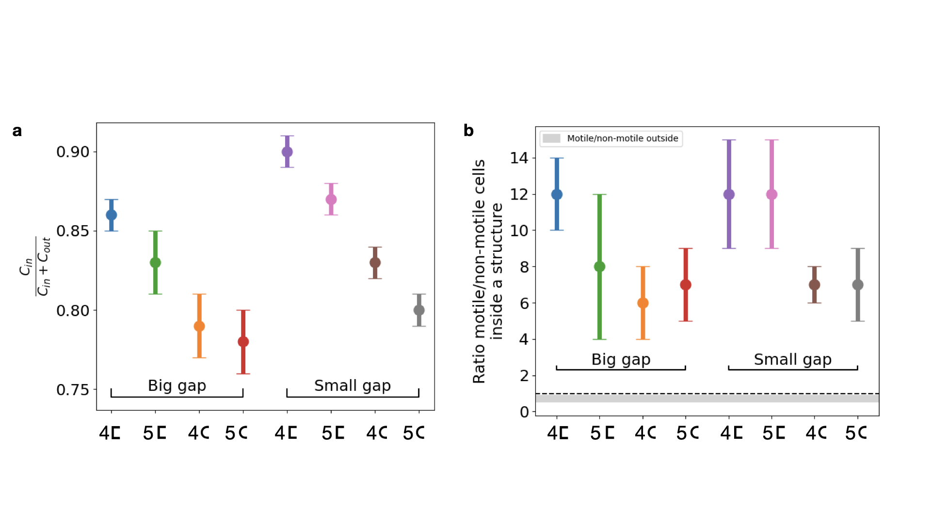
Figure 4: Relative concentrations (experiments). a. Relative concentration (averaged over 9 structures of the same kind) of motile cells between inside and outside of a structure. Error bars are standard deviations. b. Ratio (averaged over 9 structures of the same kind) between motile cells concentration and non-motile cells concentration, always inside a structure. Error bars are standard deviations. For reference the gray area represents the same ratio measured outside of the structures. The width of the gray area is the standard deviation. The dashed line marks equal concentrations (ratio $1$).

In Figure 4a we test our previous conclusions against the variability of the area of the structures as well as of (motile) sperm cell concentration in the different samples and in the different regions of the same channel. We need to rule out that results for the numbers of cells in the structure are not influenced by fluctuations of cells in the region and sample where we have performed the observation, which is known to display some (weak) variation. Plot 4a illustrates the relative concentration of motile cells $C_{r}=C_{in}/(C_{in}+C_{out})$: $C_{in}$ is the average concentration (number per unit area) of cells inside a structure, $C_{out}$ is the average concentration outside of the the structure, measured roughly in the mid distance between the structure and nearby structures (this ensures that surface effects are minimised). The relative concentration is defined to be constrained between $0$ (no trapping) to $1$ (infinite trapping), while the concentration ratio $C_{in}/C_{out}=C_{r}/(1-C_{r})$ can grow to infinite. We remark that, with cornered structures and small gaps, we get quite high values of this ratio: $C_{in}/C_{out}\sim 7-9$. The use of cornered structure is the key to get a concentration contrast much higher than the one achieved in previous studies Guidobaldi et al. (2014). The role of the curvature of walls is discussed in details in Section 3 and in the ESI where our numerical results show that, at constant physical dimensions, smaller curvatures always enhance the trapping power of structures or membranes. The effect of the number of petals $n$ going from $4$ to $5$ on the relative concentration is a reduction, of roughly a factor $\approx 1.2$ for all cases. This reduction is compatible, quantitatively, with the reduction, when going from $n=4\to n=5$, of the percentage of area occupied by petals - which have the largest trapping power - with respect to the whole structure.

The last observation we report is crucial for applications, as it concerns the ratio among motile and non-motile cells - details on their distinction are contained in the Methods section ”Distinction between motile and non-motile cells”. The efficiency of a sperm sorting technique, in fact, is determined by the concentration of motile cells. The motile/non-motile ratio, if measured outside of the structures, in the free area not too close to the outer boundaries of the trapping structures, is quite unvaried in all the observed samples, and amounts to $\sim 0.7\pm 0.2$, i.e. in the non-trapped regions the sample hosts a majority of non-motile cells. On the contrary the ratio inside the trapping structures is clearly in favour of the motile cells, see Figure 4b, with values in the range $4-15$, depending on the structure type. The larger motile/non-motile ratios are measured for cornered structures with small gaps. The ratio between motile and non-motile cells has larger errors with respect to $C_{in}/C_{out}$. The percentage of motile cells is much higher than $1$ for all the structures, the largest value are reached in those with cornered petals. This measure suggests that our mechanism acts as an efficient selectors for the motility of sperm. This result is crucial in applications that usually require not only high concentrations but also cells with high motility.

III Results: numerical

We have adopted a simplified model of the kind of “wagging” Active Brownian particles, inspired to previous studies Tasoglu et al. (2013); Guidobaldi et al. (2014). In the Methods we give the details of the model, here we describe it qualitatively in its essential aspects. Each cell is represented by its center of mass position and by the orientation of the self-propulsion direction (e.g. the tail average direction) in the plane. The orientation vector diffuses according to rotational thermal Brownian motion with a very long persistence time (unperturbed sperm cells follow straight paths longer than any characteristic length in our experiment). The cells interact with each others through a soft potential. The walls exert a harmonic elastic repulsion together with a torque that tends to align the tail orientation to a direction forming with the wall a small angle (this is in accordance with “occupied cone” models that reproduce the effective excluded volume of the long tail Elgeti et al. (2010); Denissenko et al. (2012)) . The “wagging” ingredient consists in an oscillating force perpendicular to the cell orientation with a frequency comparable to that of sperm beating Tasoglu et al. (2013); Gong et al. (2021). We have verified that all such ingredients are necessary to obtain a behavior which is coherent with our experimental observations. In particular the transversal oscillation is key to obtain a trapping power of corners which depends upon their curvature.

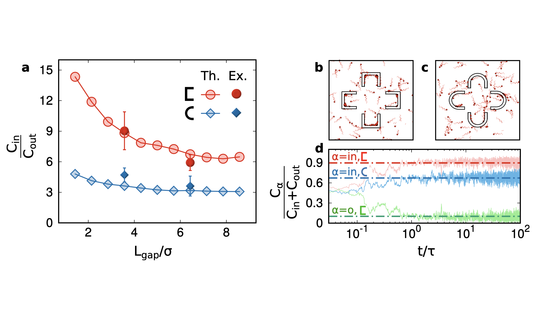
Figure 5: Results from simulations. a. Ratio between the average concentration of cells found inside and outside of a structure versus the width of the gap $L_{gap}$ (normalised by the sperm head diameter $\sigma$, see Methods); b-c. Snapshots of simulations with different structure shapes; the snake-like lines following each sperm position are obtained by tracing its motion in a short period of the transversal force oscillation (see Methods). d. Relative occupancy as a function of time, confirming that the initial concentrations are equal and then change in time, the outside concentration is slightly depleted while the inside one increases to a plateau which depends upon the petal shape.

The sizes of the structures, as well as the intrinsic properties of the sperms, such as speed, wagging frequency and persistence time, are fixed by experimental observations. The other parameters, such as the constants appearing in the repulsive potentials (for sperm-wall and sperm-sperm interactions) as well as constants in the aligning torque terms (see Methods), are fixed looking for reasonable comparison between numerical simulations and experiments for a single choice of $L_{gap}$ and shape of the petals. After the calibration of the parameters we have performed simulations with different $L_{gap}$ and different shapes of the petals, and checked that the comparison with the experiments remained good, obtaining a fair check of our assumptions (see Figure 5b,c for snapshots, see also movies attached).

The main result of our simulations is the trapping power for two kinds of pocket shape (cornered and rounded) and a wide range of gap sizes, Figure 5a. The figure demonstrates that cornered   $\sqcap$  structures are always more trapping than rounded   $\cap$  structures and that increasing the gap size reduces the trapping power. These two observations are in substantial agreement with the experiments. Remarkably, numerical simulations teach us that $L_{gap}$ is certainly a less relevant parameter than the shape of the petals. Indeed, the red curve in Fig. 5a is always above the blue curve, that is with   $\cap$  structures - whatever small is the gap size - one cannot achieve the relative concentration obtained with   $\sqcap$  structures. We recall that decreasing $L_{gap}$ at constant size of the petals implies a relative increase of the trapping surface: this is the qualitative explanation of the decreasing curves in Fig. 5a.

It is interesting to observe that in both cases an asymptotic trapping power larger than $1$ is found suggesting that even spare petals (not close in “flowers”) can be used to entrap sperms. Of course increasing much more $L_{gap}$ would result in totally open structures and the measurement, in an experiment with a single structure surrounded by infinite unconfined volume, would be dominated by bulk concentration, therefore a decrease to $1$ is expected, asymptotically: however verifying this requires much larger simulation chambers to avoid finite-size effects. We remark that such finite-size effects are present also in our experiments. It would be interesting, in future experiments, to study if the relative position or orientation of the structures with respect to the entrance can influence the filling of each structure by capillary injection. We speculate that a more dense arrangement of traps (i.e. drastically reducing the distance between them) could lead to a reduction of the trapping performance, as the original sample, being loaded from a side of the chip, would find more difficult to reach all the trapping units. Panel d of Fig. 5 is useful to evaluate the sorting time. The relative concentration, starting from a situation $C_{in}=C_{out}$, achieves an unbalanced plateau in a time $t\sim\tau$ where $\tau$ is the persistence time of the model sperm cells (see Methods). In physical time this corresponds to $\sim 100$ seconds. This result gives also a hint about the fact that the experimental measurements, taken a few minutes after the chip filling, come from a steady regime.

Numerical simulations (not shown) with single sperm cells in a pocket with different curvatures radii $R$ confirm the origin, discussed already in Guidobaldi et al. (2014), that trapping is enhanced by radii smaller than the occupied size of the sperm cell, typically head diameter $\sigma$ plus oscillation amplitude $A$, e.g. curvature with $R\ll\sigma+A$ are strongly trapping with respect to curvature with $R\gg\sigma+A$: this can be understood as a consequence of the fact that the interaction with a curved wall together with the transversal oscillation make very unlikely, for a sperm, to follow the curvature without bouncing back. On the contrary, a sperm model that has no wagging, can align close to and follow any kind of curvature without never coming back, emerging from the pocket and escaping from it. We refer to the Supplemental Movies for a rapid understanding of this scenario.

IV Conclusions

Motile cells, such as sperms or bacteria, display fascinating behavior which defies several basic aspects of the physics of mixtures realised with colloids, emulsions, suspensions etc. Segregation of different parts of a standard mixture (one made of components which are not self-motile) is usually achieved by driving the mixture through externally imposed flows (such as centrifugation at the macroscale, or pumping a flow in microfluidic devices). The same happens, in standard sorting techniques, for sperm samples Boomsma et al. (2004); Rappa et al. (2016). In this work we have taken advantage of the intrinsic motility of sperms to obtain the segregation of motile cells in small confined regions. We have explored a family of microfluidic devices where three different parameters are tuned experimentally, in order to understand which is the optimal strategy to enhance the concentration of motile sperm. We have also calibrated a simple but effective numerical model of sperm cells (including interactions between cells and between each cell and the boundaries) which reproduces the experimental results and open a virtually infinite set of future explorations for improving the designs towards other needs and applications. We have put in evidence - experimentally and theoretically - that the efficiency of our sorting method, is mainly enhanced by the specific design of surfaces. Counterintuitively, their shape, in particular, small curvatures and cornered angles, plays a more important role than the size of the entrance (gap) of the trap: our device increases the concentration of motile sperms by an order of magnitude. This has been explained in terms of the increased self-trapping mechanism caused by the interplay between cornered angles and the the peculiar swimming mechanism of sperms. The recent developments in microfluidic designing techniques offer a range of intriguing possibilities to further improve the efficiency of our trapping mechanism, for instance by manipulating the roughness of surfaces Guidobaldi et al. (2015), creating a plethora of additional angles with small curvatures.

Recent studies have already exploited microfluidics without flow-pumping for sperm sorting Nosrati et al. (2014); Xiao et al. (2021); Simchi et al. (2021). These works are somehow complementary to ours, because they focus on technology readiness of the chip and on the evalutation of DNA fragmentation, while our analysis explores the geometry of the device, looking for optimal shapes that can enhance physical effects for sorting. Moreover, the filtered sample obtained within our chip (that is the content of the trapping chambers) has a cell concentration which is higher than the original sample, that is our chip is not only a filter/sorter but also a concentrator. Our device improves also the time-efficiency of the sorting process: in our study, the sorting time is of the order of a few tens of seconds, which is smaller than the typical times needed in previous studies Nosrati et al. (2014); Xiao et al. (2021); Simchi et al. (2021). The device proposed here is low-cost, disposable if needed, easy to fabricate and use, and suitable for later integration with more complex devices for clinical applications. Moreover, it is at quite a high level of technological readiness. In the future, such a trapping device may be implemented in a multiplexed system for the purpose of picking up highly motile cells. The motile sperm cells, trapped in the microstructures, can be taken away with subsequent rinses or by providing apertures on a side of the chip and using a microscope-guided syringe to collect the concentrated sperm. For diagnostics purposes, one may imagine optical reading (through lighting levels) of the concentration in the confining region. A future development of our study concerns the correlation between sperm performance, e.g. speed or other parameters, and the features of the confining regions, which could help in designing more sophisticated chips for point-of-care diagnostic applications where a detailed spermiogram can be directly elaborated.

Our study suggests conjectural applications where oocytes are directly inserted into the trapping chambers of the chip of a microfluidic multilayered open device Oh et al. (2017): the diameter of mature oocytes, including the zona pellucida, is smaller than 150-120 $\mu m$, comparable to the diameter of the central part of our chambers, which - however - can be easily redesigned with a slightly larger internal area, if necessary. This idea could be interesting for future researches, and could also lead to a totally new in-vitro fertilisation technique, in principle more effective than conventional IVF (thanks to the high concentration of motile, already selected, sperms around the oocyte) and where the final selection of the fertilising sperm is not due to the hand of a technician/biologist, as in ICSI, but to natural competition in oocyte penetration among several tens of sperms. A further advantage of such a conjectural technique is that semen needs neither preparation nor waiting in the dish/chip for the oocytes: as soon as the oocytes are ready (e.g. after incubation and other treatments which usually take hours) they are transferred in the chip trapping chambers and only then the raw sample, just after ejaculation or thawing, is injected by capillarity in the chip: at that point in a few seconds the chambers fill up with dense concentrations of $\sim 90\%$-motile sperms, in close contact with their target.

V Methods

V.1 Lithography of the structures

Microfluidic trapping devices are fabricated using conventional soft lithography and replica molding technique from SU-8 (Microchem, YMC, Switzerland) masters. SU-8 masters are realized via standard optical lithography Zizzari et al. (2011); Chiriacò et al. (2016): a thin layer of SU-8 negative photoresist is deposited onto a clean silicon substrate and the entire patterns of ad hoc designed photomasks (J.D. Phototools Ltd., Oldham, Lancashire, UK) are transferred on the photoresist film via UV exposure. The process has been optimized to obtain a height of ($14.7\pm 0.5)\mu m$ for all the characteristic structures of the device. Each device consists of two networks of input /output microchannels connected to a microstructured chamber (Fig. 1a) in order to fullfil sperm samples by capillarity. Rectangular microfluidic channels have dimensions of $100\mu m\times 15\mu m$ and length of about $10mm$. The quasi-2D microstructured chamber has total dimension of $10mm\times 8mm\times 15\mu m$ and includes a $12\times 10$ matrix with 4 groups of different trapping units: each group contains at least 30 identical trapping units separated by an average period of about $450\mu m$. As shown in Fig. 1a the trapping area consists of a flower structure characterized by: i) a different number of “petals”, n = 4 or 5; ii) different shape of petals, rounded (R) or cornered (C); iii) different opening spaces at the base of each petal, “gap” $L_{gap}$, which are small (S, with $L_{gap}=20\mu m$) or big (B, with $L_{gap}=40\mu m$). The combination of these features creates a heterogeneous matrix for trapping analysis. The different units alternate every 3 rows of the matrix in order to ensure that they are all uniformly reached by the sperm cells via capillary motion and to collect a larger statistics in the results. Thereafter, the microfluidic trapping chips are obtained by replica molding, by casting a mixture of PDMS pre-polymer and curing agent (10: 1, Sylgard-184, Dow Corning - USA) onto one of the SU-8 masters. The PDMS is then polymerized at 140° C for 15 min and then detached from the master. To promote the imbibition, the microchannels are opened with a razor blade and the replica is placed in conformal contact with a glass substrate to allow the closure of the device. To improve sealing and displacement of cell sample, both the replica and the glass are treated with oxygen plasma (Diener Pico, low pressure plasma system: $100W$, $240cm^{3}/min$ of $O_{2}$ flow; $0.5mBar$; $60s$).

V.2 Details about sperm solution preparation

Spermatozoa samples from bulls were obtained from ”Agrilinea S.R.L” Rome, and preserved in a liquid nitrogen cylinder. The sperm samples were obtained in the form of sperms suspended in semen and packed in several vials. At the onset of the experiment, one vial of sperms was taken out of the nitrogen cylinder and immersed in a hot water bath of 37 ^∘C for 10 minutes. After 10 minutes, the vial was taken out of the bath and immediately cut open using a pair of sterilized scissors and the entire content was poured out of the vial into an Eppendorf. Using a micropipette, 50$\,\mu l$ of the sperm suspension was sucked out from the Eppendorf and inserted into the microchannel, ensuring proper filling inside the structures. The ends of the channel were then sealed. The locomotion of the sperm cells were recorded by using a digital camera (Nikon, USA) connected to an inverted microscope. During the entire duration of the experiment, the microchannel placed on the stage of the microscope was subject to a controlled temperature environment of 37 degrees centigrade using heating unit and temperature sensors. An in house software developed using Python Programming language was used to capture and analyse the images. Naked-eye cell counting has been performed on the image sequences (movies $20$ seconds long with $50$ frames per second acquisition), where each image has a $2048\times 2048$ pixels resolution and captures (at magnification $10x$) an area of $\sim 1330\times 1330\mu m^{2}$ (a matrix of $3\times 3$ structures). Counts have been repeated every $5$ seconds to ensure stability of the numbers. The occupancy of each petal or structure is defined as the average between the count in the first $5$ seconds and the count in the lat $5$ seconds. We waited $\sim 5-10$ minutes, after the chip filling, to start image acquisition: this (according also to our numerical simulations, see Fig. 4d) guarantees a stationary state.

V.3 Distinction between motile and non-motile cells

In our experimental study we have distinguished the class of motile and non-motile cells by means of a threshold on their velocity, at $1\mu m/s$. The choice of this value comes naturally from empirical evidence and is not particularly significant within a broad interval. Indeed, all our experimental observations come from $20$ seconds-long recordings, and we have a resolution of slightly less than a micron per pixel. As a consequence, when we label a cell ”non-motile”, we can conclude that it has moved less than $1$ micron in $20$ seconds, i.e. it has a speed smaller than $0.05\mu m/s$. Cells with a velocity larger than this threshold have a non-negligible velocity that can be measured with good resolution and that allows us to label a cell ”motile”. However, we have rarely observed cells slower than $10\mu m/s$, so that motile and non-motile cells are well-dinstiguished.

V.4 Model for the simulations

To reproduce our experimental findings, we model each sperm as a spherical active particle in the overdamped regime. The complex swimming mechanism of a single sperm is reproduced by effective time-dependent forces Guidobaldi et al. (2014), included in the dynamics of the center of mass position, $\mathbf{x}_{i}$:

$$\gamma\dot{\mathbf{x}}_{i}=\mathbf{F}_{i}+\mathbf{F}_{i}^{w}+\gamma v_{0}\mathbf{n}_{i}+\sqrt{2\gamma T}\,\bm{\eta}_{i}+A\omega\cos{(\omega t)}\mathbf{n}^{\perp}_{i}\,,$$ (1)

where the constant $\gamma$ is the drag coefficient and $T$ the solvent temperature. The term $\bm{\eta}_{i}$ is a white noise vector with zero average and unit variance accounting for the collisions between the solvent molecules and the active particles, such that $\langle\bm{\eta}_{i}(t)\bm{\eta}_{j}(t^{\prime})\rangle=\bm{\delta}(t-t^{\prime})\delta_{ij}$.

The particles interact through the force $\mathbf{F}_{i}=-\nabla_{i}U_{tot}$, where $U_{tot}=\sum_{i<j}U(|\mathbf{x}_{i}-\mathbf{x}_{j}|)$ is a pairwise potential. The shape $U$ is chosen as a shifted and truncated Lennard-Jones potential:

$$U(r)=4\epsilon\left[\left(\frac{\sigma}{r}\right)^{12}-\left(\frac{\sigma}{r}\right)^{6}\right]\,,$$ (2)

for $r\leq 2^{1/6}\sigma$ and zero otherwise. The constants $\epsilon$ and $\sigma$ determine the energy unit and the nominal particle diameter, respectively. The term $\mathbf{F}_{i}^{w}$ represents the repulsive force exerted by the obstacles, whose properties will be specified later.

The effects of the flagella are modeled by the active force, $\gamma v_{0}\mathbf{n}_{i}$, evolving according to the active Brownian particles (ABP) dynamics. In the ABP model, the active force acts locally on each particle, providing a constant swim velocity $v_{0}$ and a time-dependent orientation, $\mathbf{n}_{i}=(\cos{\theta_{i}},\sin{\theta_{i}})$. The orientational angle $\theta_{i}$ evolves stochastically via a Brownian motion:

$$\dot{\theta}_{i}=\sqrt{2D_{r}}\chi_{i}+T_{i}^{w}\,,$$ (3)

where $\chi_{i}$ is a white noise with zero average and unit variance and $D_{r}=1/\tau$ determines the persistence time of the active force. $T_{i}^{w}$ is the torque exerted by the wall whose properties will be explained in detail later.

The last term in the right hand side of Eq. (1) is a periodic time-dependent force which mimics the oscillations of the sperm head because the vector $\mathbf{n}^{\perp}=(-\sin{\theta},\cos{\theta})$ points perpendicularly to the swimming direction $\mathbf{n}_{i}$. The constants $A$ and $\omega=2\pi\nu_{i}$ determine the amplitude and the frequency of the oscillations, respectively.

V.4.1 Force and torque exerted by the walls

Each wall is described by a continuous closed line in the plane, representing its perimeter, which in some parts is external to the structure and in some other parts is internal. Locally (near the point of contact) it can always be written as $y=w(x)$ and/or $x=w(y)$. Let us consider one of the two cases (the first), while the other is obtained by simply exchanging $x$ with $y$. In the first case the force exerted by the wall reads:

$$\mathbf{F}^{w}=-U^{\prime}(w(x)-y)\mathbf{e}\,,$$ (4)

where $\mathbf{e}=(w^{\prime}(x),-1)/\sqrt{1+w^{\prime}(x)^{2}}$ is the unit vector orthogonal to the wall profile and $U_{w}(r)$ is chosen as a harmonic repulsive potential truncated in its minimum:

$$U_{w}(r)=\frac{K}{2}r^{2}\Theta(r)\,,$$

where $K$ determines the strength of the potential and $\Theta(r)$ is the Heaviside step-function.

The torque exerted by the walls, $T^{w}_{i}$, reads:

$$T^{w}_{i}({\theta,r,\phi})= -I(\theta,\phi)\,\ell_{0}|\mathbf{F}_{w}|\sin[2(\theta-\phi\pm\alpha)]\,$$ (5)

where the angle $\phi$ defines the orientation of the wall and is defined as

$$\phi=\psi+\frac{\pi}{2}$$

being $\psi$ the angle formed by the outward normal with respect to the $\hat{\mathbf{x}}$ axis. The function $I$ selects the interval of $\theta$ which activates the torque, namely when the self-propulsion vector points inward with respect to the wall profile. The torque aligns the particle orientation to the orientation of the wall so that an angle $\pm\alpha$ (the sign is determined by the orientation) is formed. This assumption is consistent with experimental results since each sperm usually does not swim parallel to the wall but forms a relative angle of $\approx 10$ degree Elgeti et al. (2010); Denissenko et al. (2012); Bettera Marcat et al. (2020). We remark that the torque ingredient is fundamental to avoid accumulation of particles (without sliding) close to the wall, as it is observed in simulations without torque Caprini et al. (2020).

V.4.2 Simulation parameters & geometrical setup

The typical size of the particle is chosen as $\sigma=6\mu m$, and accounts for the effective volume occupied by the head of each sperm, which is approximated as a disk. The persistence time is $\tau=10^{2}s$, while the swim velocity $v_{0}=30\mu m/s$. The parameters of the thermal bath, $\gamma$ and $T$ gives rise to a diffusion coefficient $D_{t}=10^{2}\mu m^{2}/s$ much smaller than the effective diffusivity due to the active force, $D_{a}=v^{2}_{0}\tau=9\times 10^{4}\mu m^{2}/s$, as it usually happens for self-propelled particles Bechinger et al. (2016). Finally, amplitude and frequency of the head oscillation read $A=3.5\mu m$ and $\nu=30/(2\pi)s^{-1}$, respectively, in agreement with Ref. Guidobaldi et al. (2014). The energy scale of the interaction is chosen as $\epsilon=1\mu m^{2}/s^{2}$, while the parameters of force and torque of each wall are $K=10^{3}\mu/s^{2}$, $\ell_{0}=6\mu m^{2}/s^{2}$ and $\alpha=10$ degree.

Simulations are performed using dimensionless units, rescaling time and position through the time scale introduced by the active force and size of the sperm, namely $\bar{t}=t/\tau$ and $\bar{x}=x/\sigma$.

The numerical study is performed by simulating a system of $N=100$ (not far from the average total number of particles in a similar area of the experiments) interacting particles in a box of size $L_{0}$ with periodic boundary conditions. In Fig. 6 we show the simulation setup with the symbols representing the fundamental lengths of the simulations. In units of the sperm head’s diameter $\sigma$ we have used $L_{1}=5$, $L_{3}=16$, $L_{2}=L_{3}/2+L_{1}=13$, and $L_{0}=64+\sqrt{2}L_{gap}$, while the width of the walls is $H=2$, and clearly the radius of the half-circle representing the curved part of the petals is $L_{3}/2$.

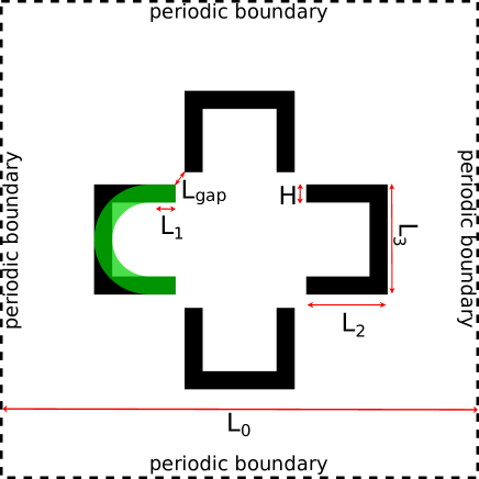
Figure 6: Setup of the simulations whose results are presented in Fig. 4. The sizes, given in units of $\sigma$ (the particle diameter, ideally corresponding to the head of the sperm cell) are $L_{1}=5$, $L_{3}=16$, $L_{2}=L_{3}/2+L_{1}=13$, and $L_{0}=64+\sqrt{2}L_{gap}$, while the width of the walls is $H=2$, and the radius of the half-circle representing the curved part of the petals is $L_{3}/2$. The value of $L_{gap}$ is varied between $1$ and $9$ (again in units of $\sigma$), as shown in Fig. 5.

Author Contributions

B. N., A.P., C. M., R. D. L. and I. V. conceived the idea and planned the experiments. I.V., A. Z. and V. A. designed and provided the microstructured devices. C. M., B. N. and I. V. performed the experiments. C. M., B. N. and A. P. carried out the experimental data analysis. L.C. performed the numerical simulations and their analysis. All the Authors contributed to the writing of the manuscript.

Conflicts of interest

There are no conflicts to declare’.

References

- Barratt et al. (2009) C. L. Barratt, V. Kay and S. K. Oxenham, J. Biol., 2009, 8, 1.
- Frey (2010) K. A. Frey, Prim. Care, 2010, 37, 643.
- Friedrich and Jülicher (2007) B. M. Friedrich and F. Jülicher, Proc. Natl. Acad. Sci. U.S.A., 2007, 104, 13256.
- Friedrich et al. (2010) B. M. Friedrich, I. H. Riedel-Kruse, J. Howard and F. Jülicher, J. Exp. Biol., 2010, 213, 1226.
- Gaffney et al. (2011) E. A. Gaffney, H. Gadêlha, D. J. Smith, J. R. Blake and J. C. Kirkman-Brown, Annu. Rev. Fluid Mech., 2011, 43, 501.
- Guasto et al. (2020) J. S. Guasto, J. B. Estrada, F. Menolascina, L. J. Burton, M. Patel, C. Franck, A. Hosoi, R. K. Zimmer and R. Stocker, J. R. Soc. Interface, 2020, 17, 20200525.
- Schill et al. (2010) W.-B. Schill, F. H. Comhaire, T. B. Hargreave, A. Lenzi and A. M. Isidori, Andrologia clinica, Springer, 2010.
- Boomsma et al. (2004) C. M. Boomsma, M. J. Heineman, B. J. Cohlen and C. M. Farquhar, Cochrane Database Syst. Rev., 2004, CD004507.
- Zini et al. (2000) A. Zini, A. Finelli, D. Phang and K. Jarvi, Urology, 2000, 56, 1081.
- Rappa et al. (2016) K. L. Rappa, H. F. Rodriguez, G. C. Hakkarainen, R. M. Anchan, G. L. Mutter and W. Asghar, Biotechnol. Adv., 2016, 34, 578.
- Smith and Takayama (2017) G. D. Smith and S. Takayama, Mol Hum Reprod, 2017, 23, 257.
- Han et al. (2010) C. Han, Q. Zhang, R. Ma, L. Xie, T. Qiu, L. Wang, K. Mitchelson, J. Wang, G. Huang, J. Qiao et al., Lab Chip, 2010, 10, 2848.
- Matsuura et al. (2013) K. Matsuura, T. Uozumi, T. Furuichi, I. Sugimoto, M. Kodama and H. Funahashi, Fertil. Steril., 2013, 99, 400.
- Chen et al. (2013) C.-Y. Chen, T.-C. Chiang, C.-M. Lin, S.-S. Lin, D.-S. Jong, V. F.-S. Tsai, J.-T. Hsieh and A. M. Wo, Analyst, 2013, 138, 4967.
- Tasoglu et al. (2013) S. Tasoglu, H. Safaee, X. Zhang, J. L. Kingsley, P. N. Catalano, U. A. Gurkan, A. Nureddin, E. Kayaalp, R. M. Anchan, R. L. Maas et al., Small, 2013, 9, 3374.
- Huang et al. (2015) H.-Y. Huang, H.-H. Shen, L.-Y. Chung, Y.-H. Chung, C.-C. Chen, C.-H. Hsu, S.-K. Fan and D.-J. Yao, IEEE Trans Nanobioscience, 2015, 14, 857.
- Knowlton et al. (2015) S. M. Knowlton, M. Sadasivam and S. Tasoglu, Trends Biotechnol., 2015, 33, 221.
- Hussain et al. (2016) Y. H. Hussain, J. S. Guasto, R. K. Zimmer, R. Stocker and J. A. Riffell, J. Exp. Biol., 2016, 219, 1458.
- Zaferani et al. (2019) M. Zaferani, G. D. Palermo and A. Abbaspourrad, Sci. Adv., 2019, 5, eaav2111.
- Cho et al. (2003) B. S. Cho, T. G. Schuster, X. Zhu, D. Chang, G. D. Smith and S. Takayama, Anal. Chem., 2003, 75, 1671.
- Schuster et al. (2003) T. G. Schuster, B. Cho, L. M. Keller, S. Takayama and G. D. Smith, Reprod. Biomed. Online, 2003, 7, 75.
- Nosrati et al. (2014) R. Nosrati, M. Vollmer, L. Eamer, M. C. San Gabriel, K. Zeidan, A. Zini and D. Sinton, Lab Chip, 2014, 14, 1142.
- Asghar et al. (2014) W. Asghar, V. Velasco, J. L. Kingsley, M. S. Shoukat, H. Shafiee, R. M. Anchan, G. L. Mutter, E. Tüzel and U. Demirci, Adv. Healthc. Mater., 2014, 3, 1671.
- Shirota et al. (2016) K. Shirota, F. Yotsumoto, H. Itoh, H. Obama, N. Hidaka, K. Nakajima and S. Miyamoto, Fertil. Steril., 2016, 105, 315–321.
- Xiao et al. (2021) S. Xiao, J. Riordon, M. Simchi, A. Lagunov, T. Hannam, K. Jarvi, R. Nosrati and D. Sinton, Lab on a Chip, 2021, 21, 775–783.
- Simchi et al. (2021) M. Simchi, J. Riordon, J. B. You, Y. Wang, S. Xiao, A. Lagunov, T. Hannam, K. Jarvi, R. Nosrati and D. Sinton, Lab on a Chip, 2021, 21, 2464–2475.
- Agarwal et al. (2016) A. Agarwal, A. Borges Jr and A. Setti, Non-invasive sperm selection for in vitro fertilization, Springer, 2016.
- Lu et al. (2010) J.-C. Lu, Y.-F. Huang and N.-Q. Lü, Zhonghua nan ke xue = Natl. j. androl., 2010, 16, 867.
- Graham (2001) J. K. Graham, Anim. Reprod. Sci., 2001, 68, 239.
- Zheng et al. (2011) G. Zheng, S. A. Lee, Y. Antebi, M. B. Elowitz and C. Yang, Proc. Natl. Acad. Sci. U.S.A., 2011, 108, 16889.
- Elgeti et al. (2015) J. Elgeti, R. G. Winkler and G. Gompper, Rep. Prog. Phys., 2015, 78, 056601.
- Nosrati et al. (2015) R. Nosrati, A. Driouchi, C. M. Yip and D. Sinton, Nature Communications, 2015, 6, 8703.
- Rode et al. (2019) S. Rode, J. Elgeti and G. Gompper, New J. Phys., 2019, 21, 013016.
- Rothschild (1963) Rothschild, Nature, 1963, 198, 1221.
- Li et al. (2008) G. Li, L.-K. Tam and J. X. Tang, Proc. Natl. Acad. Sci. U.S.A., 2008, 105, 18355–18359.
- Smith et al. (2009) D. Smith, E. Gaffney, J. Blake and J. Kirkman-Brown, J. Fluid Mech., 2009, 621, 289–320.
- Elgeti et al. (2010) J. Elgeti, U. B. Kaupp and G. Gompper, Biophys. J., 2010, 99, 1018.
- Magdanz et al. (2015) V. Magdanz, B. Koch, S. Sanchez and O. G. Schmidt, Small, 2015, 11, 781.
- Denissenko et al. (2012) P. Denissenko, V. Kantsler, D. J. Smith and J. Kirkman-Brown, Proc. Natl. Acad. Sci. U.S.A., 2012, 109, 8007.
- Guidobaldi et al. (2014) A. Guidobaldi, Y. Jeyaram, I. Berdakin, V. V. Moshchalkov, C. A. Condat, V. I. Marconi, L. Giojalas and A. V. Silhanek, Phys. Rev. E, 2014, 89, 032720.
- Paoluzzi et al. (2020) M. Paoluzzi, L. Angelani and A. Puglisi, Phys. Rev. E, 2020, 102, 042617.
- Yaghoobi et al. (2021) M. Yaghoobi, M. Azizi, A. Mokhtare and A. Abbaspourrad, Lab Chip, 2021, 21, 2791.
- Galajda et al. (2007) P. Galajda, J. Keymer, P. Chaikin and R. Austin, J. Bacteriol. Res., 2007, 189, 8704–8707.
- Angelani et al. (2011) L. Angelani, A. Costanzo and R. Di Leonardo, EPL, 2011, 96, 68002.
- Koumakis et al. (2013) N. Koumakis, A. Lepore, C. Maggi and R. Di Leonardo, Nat. Commun., 2013, 4, 1.
- Koumakis et al. (2014) N. Koumakis, C. Maggi and R. Di Leonardo, Soft matter, 2014, 10, 5695.
- Makse et al. (1997) H. A. Makse, S. Havlin, P. R. King and H. E. Stanley, Nature, 1997, 386, 379.
- Di Leonardo et al. (2010) R. Di Leonardo, L. Angelani, D. Dell’Arciprete, G. Ruocco, V. Iebba, S. Schippa, M. P. Conte, F. Mecarini, F. De Angelis and E. Di Fabrizio, Proc. Natl. Acad. Sci. U.S.A., 2010, 107, 9541.
- McCandlish et al. (2012) S. R. McCandlish, A. Baskaran and M. F. Hagan, Soft Matter, 2012, 8, 2527.
- Gnoli et al. (2013) A. Gnoli, A. Petri, F. Dalton, G. Pontuale, G. Gradenigo, A. Sarracino and A. Puglisi, Phys. Rev. Lett., 2013, 110, 120601.
- Medina-Sánchez et al. (2016) M. Medina-Sánchez, L. Schwarz, A. K. Meyer, F. Hebenstreit and O. G. Schmidt, Nano Lett., 2016, 16, 555.
- Chen et al. (2018) C. Chen, X. Chang, P. Angsantikul, J. Li, B. Esteban-Fernández de Ávila, E. Karshalev, W. Liu, F. Mou, S. He, R. Castillo et al., Adv. Biosyst., 2018, 2, 1700160.
- Striggow et al. (2020) F. Striggow, M. Medina-Sánchez, G. K. Auernhammer, V. Magdanz, B. M. Friedrich and O. G. Schmidt, Small, 2020, 16, 2000213.
- Nosrati et al. (2016) R. Nosrati, P. J. Graham, Q. Liu and D. Sinton, Sci. Rep., 2016, 6, 1.
- Xia and Whitesides (1998) Y. Xia and G. M. Whitesides, Annu. Rev. Mater. Sci., 1998, 28, 153.
- Viola et al. (2005) I. Viola, D. Pisignano, R. Cingolani and G. Gigli, Anal. Chem., 2005, 77, 591.
- Zizzari et al. (2019) A. Zizzari, M. Bianco, E. Perrone, M. Manera, S. Cellamare, S. Ferorelli, R. Purgatorio, A. Scilimati, A. Tolomeo, V. Dimiccoli et al., Chem. Eng. Process.: Process Intensif., 2019, 141, 107539.
- Zizzari et al. (2014) A. Zizzari, M. Bianco, R. Miglietta, L. del Mercato, M. Carraro, A. Sorarù, M. Bonchio, G. Gigli, R. Rinaldi, I. Viola et al., Lab Chip, 2014, 14, 4391.
- Note (1) Our observations of Fig. 2 indicate a compatibility of cell count fluctuations with Gaussian statistics, justifying the uses of t-test. We have also confirmed our results through a non-parametric Mann-Whitney test.
- Gong et al. (2021) A. Gong, S. Rode, G. Gompper, U. B. Kaupp, J. Elgeti, B. Friedrich and L. Alvarez, Eur. Phys. J. E, 2021, 44, 1.
- Guidobaldi et al. (2015) H. A. Guidobaldi, Y. Jeyaram, C. Condat, M. Oviedo, I. Berdakin, V. Moshchalkov, L. C. Giojalas, A. Silhanek and V. I. Marconi, Biomicrofluidics, 2015, 9, 024122.
- Oh et al. (2017) S. Oh, H. Ryu, D. Tahk, J. Ko, Y. Chung, H. K. Lee, T. R. Lee and N. L. Jeon, Lab on a Chip, 2017, 17, 3405–3414.
- Zizzari et al. (2011) A. Zizzari, V. Arima, A. Zacheo, G. Pascali, P. Salvadori, E. Perrone, D. Mangiullo and R. Rinaldi, Microelectron. Eng., 2011, 88, 1664.
- Chiriacò et al. (2016) M. S. Chiriacò, M. Bianco, F. Amato, E. Primiceri, F. Ferrara, V. Arima and G. Maruccio, Microelectron. Eng., 2016, 164, 30.
- Bettera Marcat et al. (2020) M. A. Bettera Marcat, M. N. Gallea, G. L. Miño, M. A. Cubilla, A. J. Banchio, L. C. Giojalas, V. I. Marconi and H. A. Guidobaldi, Biomicrofluidics, 2020, 14, 024108.
- Caprini et al. (2020) L. Caprini, F. Cecconi, C. Maggi and U. M. B. Marconi, Phys. Rev. Res., 2020, 2, 043359.
- Bechinger et al. (2016) C. Bechinger, R. Di Leonardo, H. Löwen, C. Reichhardt, G. Volpe and G. Volpe, Rev. Mod. Phys., 2016, 88, 045006.