CD and PMD Effect on Cyclostationarity-Based Timing Recovery for Optical Coherent Receivers

Abstract

Timing recovery is critical for synchronizing the clocks at the transmitting and receiving ends of a digital coherent communication system. The core of timing recovery is to determine reliably the current sampling error of the local digitizer so that the timing circuit may lock to a stable operation point. Conventional timing phase detectors need to adapt to the optical fiber channel so that the common effects of this channel, such as chromatic dispersion (CD) and polarization mode dispersion (PMD), on the timing phase extraction must be understood. Here we exploit the cyclostationarity of the optical signal and derive a model for studying the CD and PMD effect. We prove that the CD-adjusted cyclic correlation matrix contains full information about timing and PMD, and the determinant of the matrix is a timing phase detector immune to both CD and PMD. We also obtain other results such as a completely PMD-independent CD estimator, etc. Our analysis is supported by both simulations and experiments over a field implemented optical cable.

I Introduction

Timing recovery plays a critical role in the digital signal processing (DSP) chain of optical coherent receivers for synchronizing the local clock to the incoming data stream [1, 2, 3]. The core of timing recovery is a timing phase detector (TPD), which identifies the current sampling phase of the receiver analog-to-digital convertor (ADC) [4], often equivalent to detecting the phase of a generated clock tone at the frequency equal to the signal baudrate. The core can also be a timing error detector (TED), which produces error signals indicating the deviation of current sampling instance from the optimal sampling point. While finding a proper TPD or TED is a classic problem in digital communication systems, and there are numerous methods for solving it [5, 6, 7], one should pay attention to various fiber channel effects on the existing timing recovery solutions in optical communications [8]. Such effects include fiber chromatic dispersion (CD), state of polarization (SOP) rotation, polarization mode dispersion (PMD), and fiber nonlinearity, etc. Considerable efforts have been made to understand the CD and PMD effect on the timing recovery [9, 10]. It appears however that there are still more to discover especially concerning the spectral correlation involving the two data-carrying polarizations. Both CD and PMD effects can be accounted for and simple TED algorithms can be derived from the the so-called cyclic correlation matrix. In particular, we prove that the determinant of the proper matrix is a valid TPD regardless of the CD and PMD conditions of optical fiber and hence can be performed before CD and PMD equalization in the DSP chain. More analysis on the spectral correlation properties of the common timing recovery methods can also found in [11, 12].

The effect of CD on timing recovery is static and hence it is a common practice to extract timing phase after CD equalization. Because the clock tone is sensitive to CD, it also becomes a popular way to estimate the CD based on the magnitude of clock tone [13]. In contrast, the PMD effect is dynamic and the half symbol first-order differential group delay (DGD) rotated by 45-degree is well identified as the worst case for timing recovery. In fact, based on our analysis in this paper, the worst cases correspond to the slow principal state of polarization (PSP) of optical fiber lying in the $s_{2}$-$s_{3}$ plane of Stokes space (Section III-A). It then follows that one could rotate the signal polarization away from the worst case scenario prior to the timing recovery. Previous studies include adaptive polarization rotation to maximize the time-averaged error signals of Gardner TED [10], adaptive phase and/or polarization rotation to maximize cost functions similar as the clock-tone strength [14, 15], SOP rotation to minimize the correlation between two polarizations [16]. Other timing phase extraction points such as the output of channel equalizer and carrier recovery are discussed in [17].

It has been understood that the PMD effect is related to the polarization correlation. However, we haven’t seen a complete analysis on what exactly the relation is and its impact on the timing recovery. In this paper, we prove that the spectral correlation and the cyclic correlation functions are powerful tools for analyzing the channel effects on the timing recovery. We analyze in detail the CD and PMD effect on the class of timing error detectors based on the second-order cyclostationarity of data-carrying signals. We have proposed several algorithms in that class including the a completely PMD-insensitive CD estimator, a PMD matrix estimator, the DGD and PSP vector estimation, and the TED for negligible DGD, for DGD smaller that half unit interval, and for all channel conditions. We corroborate our findings with numerical simulations of an optical coherent communication system exploiting the polarization division multiplexed 16-ary quadrature amplitude modulation (PDM-16QAM) and field tests with a 153 km subterranean optical cable.

II Principle of Timing Recovery

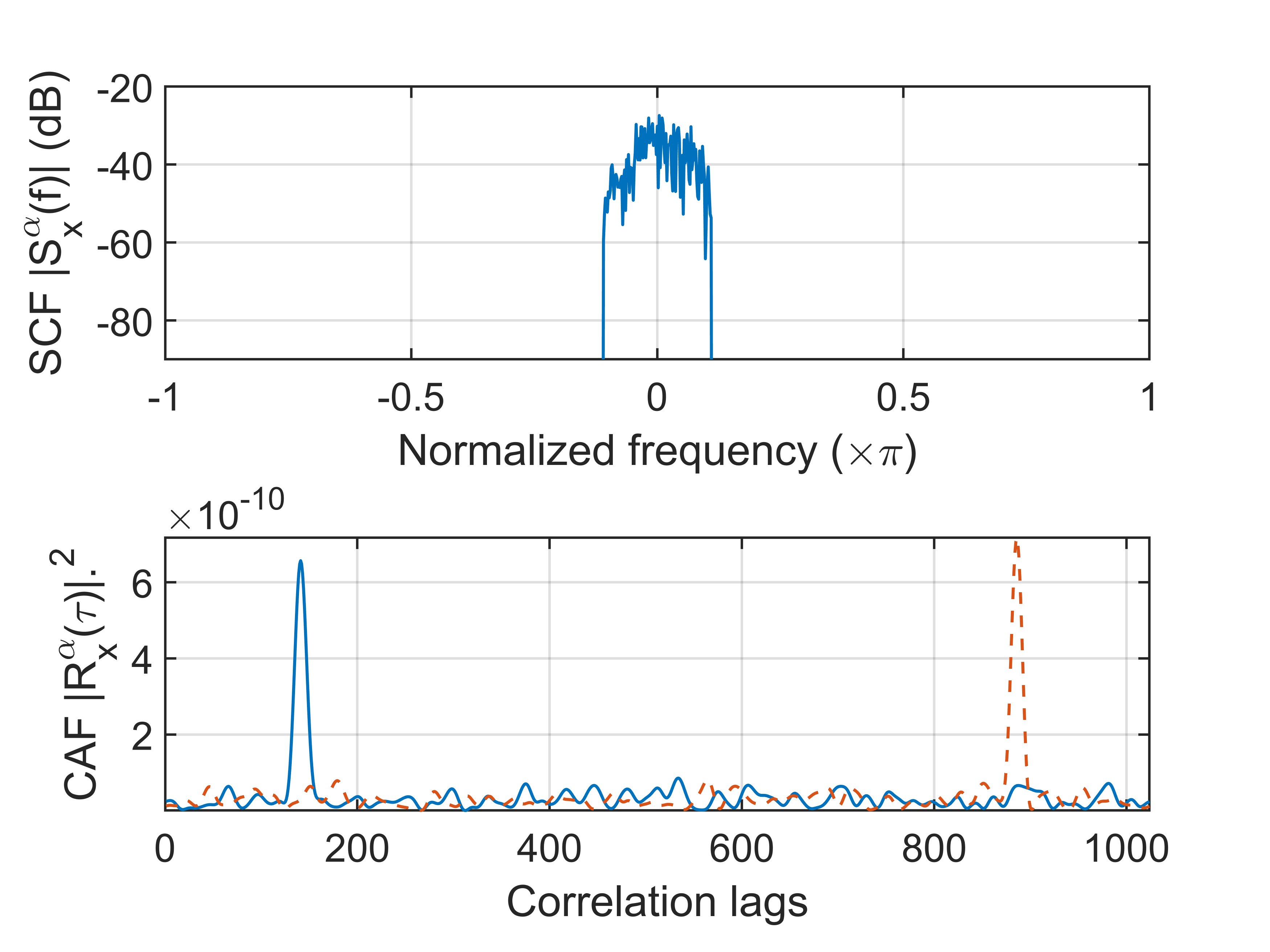
Figure 1: Simulation results of SCF and CAF based on a 32 GBaud PDM-16QAM system with the cyclic frequency equal to the baudrate, 18 dB OSNR, 100 kHz laser linewidth, $\pm$8.5 ns/nm CD, and 512 symbols. The CAF curve of dashed line is for the CD with negative sign.

Consider the general linear modulation carried by one of two orthogonal polarizations ($x$ polarization) of light

$$x(t)=\sum_{n=-\infty}^{\infty}a_{n}g(t-\tau_{g}-nT_{0})$$ (1)

where $\{a_{n}\}$ are the complex-valued symbols randomly selected from a signal constellation, $T_{0}$ is one symbol duration, $g(t)$ is the real-valued pulse shaping function, and $\tau_{g}$ is the group delay causing the varying timing phase. The signal $y(t)$ at the $y$ polarization is defined similarly but with symbols $\{b_{n}\}$ that are uncorrelated with $\{a_{n}\}$. The cyclic autocorrelation function (CAF) of $x$ is given by

$$R_{x}^{\alpha}(\tau) =\frac{1}{T_{0}}\int_{-T_{0}/2}^{T_{0}/2}E\left\{x\left(t+\frac{\tau}{2}\right)x^{*}\left(t-\frac{\tau}{2}\right)e^{-j2\pi\alpha t}\right\}\,dt$$ (2)

$$=\frac{1}{T_{0}^{2}}\int_{-\infty}^{\infty}g\left(t-\tau_{g}+\frac{\tau}{2}\right)g\left(t-\tau_{g}-\frac{\tau}{2}\right)e^{-j2\pi\alpha t}\,dt$$ (3)

where $j=\sqrt{-1}$, $E\{\cdot\}$ is the expectation operator and the cyclic frequency $\alpha$ is an integer multiple of the signal baudrate. The spectral correlation function (SCF) of $x$ can be found as the Fourier transform of the CAF

$$S_{x}^{\alpha}(f) =\int_{-\infty}^{\infty}R_{x}^{\alpha}e^{-j2\pi f\tau}\,d\tau$$ (4)

$$=\frac{1}{T_{0}^{2}}G\left(f+\frac{\alpha}{2}\right)G^{*}\left(f-\frac{\alpha}{2}\right)e^{-j2\pi\alpha\tau_{g}}\,,$$ (5)

which can be viewed as a generalization of ordinary power spectral density (a special case of SCF with $\alpha=0$). When the pulse shaping $g(t)$ is an even and real function, its Fourier transform $G(f)$ is also even and real. Also, when $G(f)$ is bandlimited with a nonzero excess bandwidth, the SCF is nonzero only for a few cyclic frequencies. Fig. 1 shows simulated SCF and CAF curves for a common modulation format used in coherent optical systems. The fiber CD caused the shift of CAF peak, which is explained in more detail in Section IV. Moreover, it is easy to verify the spectral correlation is perfect for common digital modulations in the sense that the correlation coefficient $S_{x}^{\alpha}(f)/\sqrt{S_{x}(f+\alpha/2)S_{x}(f-\alpha/2)}$ has modulus one for $\alpha\neq 0$. The spectral components that are separated by $\alpha$ are effectively carrying the same information. Note that in contrast to the real-valued power spectral density, the SCF is in general complex-valued due to the presence of phase term involving $\tau_{g}$ for $\alpha\neq 0$. This is the reason that enables us to retrieve the timing phase term by averaging the SCF with $\alpha=1/T_{0}$, the baudrate, over a certain range of frequency. That is $\int S_{x}^{\alpha}\,df=A\cdot e^{-j2\pi\alpha\tau_{g}}$ according to (5), where $A$ is a real-valued coefficient. The integration range is usually small around the zero frequency such that we compute effectively the correlation between upper and lower bands of the signal around $f=\pm 1/(2T_{0})$. It is obvious that the real and the imaginary part follows

$$\operatorname{Re}{\int S_{x}^{\alpha}\,df} =A\cdot\cos(2\pi\alpha\tau_{g})$$ (6)

$$\operatorname{Im}{\int S_{x}^{\alpha}\,df} =-A\cdot\sin(2\pi\alpha\tau_{g})$$ (7)

where the imaginary part forms the well-known timing error indicator (or detector) of Godard’s method [5]. By using (4), we obtain easily the timing error detector

$$e_{T} =-\operatorname{Im}{\int S_{x}^{\alpha}\,df}=-\operatorname{Im}R_{x}^{\alpha}(0)$$ (8)

$$=-\operatorname{Im}\left\{\frac{1}{T}\int_{-T/2}^{T/2}x(t)x^{*}(t)e^{-j2\pi\alpha t}\,dt\right\}\,,$$ (9)

where we have replaced the expectation with time average over a large $T$. The last line is recognized as the square timing error detector [7] which computes the complex coefficient of the spectral line of $|x|^{2}$ at frequency $\alpha=1/T_{0}$. It can be shown [18] that in order to maximize the SNR of the spectral line, $x(t)$ needs to be the matched filtered signal at the receiver. The TED is usually embedded in a feedback loop which adjusts the ADC sampling phase constantly to lock on the optimal timing instances.

III PMD Effect

The formulation (2–5) works equally well for the $y$ polarization. Also, the cyclic cross-correlation function (CCF) and the SCF between the two orthogonal polarizations can be similarly developed. They can be written as matrices of form

$$C(\tau)=\begin{bmatrix}R_{xx}^{\alpha}&R_{xy}^{\alpha}\\ R_{yx}^{\alpha}&R_{yy}^{\alpha}\end{bmatrix}\qquad S(f)=\begin{bmatrix}S_{xx}^{\alpha}&S_{xy}^{\alpha}\\ S_{yx}^{\alpha}&S_{yy}^{\alpha}\end{bmatrix}$$ (10)

where $R_{yx}^{\alpha}$ and $R_{xy}^{\alpha}$ are given respectively by replacing in (2) the first and the second $x(t)$ by $y(t)$. In ideal cases (i.e., no CD, no PMD, and stationary noise), the $S$ matrix is (up to a common phase term) an identity matrix, $S=e^{-j2\pi\alpha\tau_{g}}I$, at a given frequency because the data carried by $x$ and $y$ polarization are uncorrelated. Hence, according to (8), the CAF matrix

$$C(0)=\int S(f)\,df=Ae^{-j2\pi\alpha\tau_{g}}I\,,$$ (11)

where $A$ is a real-valued coefficient.

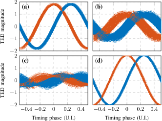
Figure 2: Characteristic curves of timing error detector derived from (a) $\operatorname{trace}(\bar{P^{\prime}})$ [equ. (20)] with $5$ ps DGD, (b) $P^{\prime}_{xx}$ with $5$ ps DGD, (c) $\operatorname{trace}(\bar{P^{\prime}})$ [equ. (20)] with $14$ ps DGD, and (d) $\operatorname{trace}(\bar{P^{\prime}U^{H}})$ [equ. (21)] with $14$ ps DGD. Solid lines: Imaginary part, $-\operatorname{Im}\{\cdot\}$. Broken lines: Real part, $\operatorname{Re}\{\cdot\}$. Simulation parameters: $32$ GBaud PM-16QAM, $20$ dB OSNR, $100$ kHz laser linewidth with no carrier frequency offset, FFT size $1024$ samples ($2$ samples per symbol), random polarization rotation.

When considering only the first-order PMD of optical fiber with no CD, we describe the change of output polarization state $E$ given the same input state over angular frequency $\omega$ by the first-order differential equation

$$\frac{dE}{d\omega}=-j(\tau_{g}+H)E\,,$$ (12)

where the matrix $H$ is Hermitian when the polarization dependent loss (PDL) is neglected. It represents the rotation of output Stokes vector about the principal state of polarization (PSP) when frequency changes. The rotation rate is precisely the differential group delay (DGD). The input polarization states are the same at the two frequencies $f\pm\alpha/2$ due to the complete spectral correlation. Therefore, when neglecting PDL, a constant unitary matrix $U$ (PMD matrix) relates the spectral components as follows

$$\underbrace{\begin{bmatrix}X(f+\alpha/2)\\ Y(f+\alpha/2)\end{bmatrix}}_{E^{\prime}_{1}}=e^{-j\phi_{0}}U\underbrace{\begin{bmatrix}X(f-\alpha/2)\\ Y(f-\alpha/2)\end{bmatrix}}_{E^{\prime}_{2}}\,,$$ (13)

where $\phi_{0}=2\pi\alpha\tau_{g}$ is the common phase induced by the group delay, $E^{\prime}_{1,2}$ are Jones vectors, $X$ and $Y$ are respectively the Fourier transform of time truncated $x(t)$ and $y(t)$ at the receiver. The PMD matrix can be written in the form

$$U=\begin{bmatrix}a&-b^{*}\\ b&a^{*}\end{bmatrix}\quad\text{with }aa^{*}+bb^{*}=1\,,$$ (14)

and admits the expansion

$$U=\cos(\pi\alpha\tau_{\text{DGD}})I-j\sin(\pi\alpha\tau_{\text{DGD}})[\vec{p}\cdot\vec{\sigma}]\,,$$ (15)

where $\vec{p}=[p_{1},p_{2},p_{3}]$ is the slow PSP Stokes vector associated with the eigenvalue $\rho=e^{-j\pi\alpha\tau_{\text{DGD}}}$ of $U$, $\vec{\sigma}=[\sigma_{1},\sigma_{2},\sigma_{3}]$ are the three Pauli matrices

$$\sigma_{1}=\begin{bmatrix}1&0\\ 0&-1\end{bmatrix},\sigma_{2}=\begin{bmatrix}0&1\\ 1&0\end{bmatrix},\sigma_{3}=\begin{bmatrix}0&-j\\ j&0\end{bmatrix}\,,$$ (16)

and $\vec{p}\cdot\vec{\sigma}=p_{1}\sigma_{1}+p_{2}\sigma_{2}+p_{3}\sigma_{3}$,

Figure 3: Characteristic curves of timing error detector derived from (a) $P^{\prime}_{xx}$, (b) $\operatorname{trace}(\bar{P^{\prime}})$ [equ. (20)], (c) $\operatorname{trace}(\bar{P^{\prime}U^{H}})$ [equ. (21)], and (d) $\operatorname{det}(\bar{P^{\prime}})$ [equ. (25)] when the DGD is $15.63$ ps. Solid lines: Imaginary part, $-\operatorname{Im}\{\cdot\}$. Broken lines: Real part, $\operatorname{Re}\{\cdot\}$. Other simulation conditions are the same as those for Fig. 2.

III-A Cyclic Periodogram

Let $E_{1,2}$ be the two output Jones vectors at frequencies $f\pm\alpha/2$ when this is no PMD and polarization rotation. Namely, they should coincide with their input states except for a common phase change. Using the relations $E_{1}=e^{-j\phi_{0}}E_{2}$, $E^{\prime}_{2}=VE_{2}$ and (13), we obtain the cyclic periodogram

$$P^{\prime}=E^{\prime}_{1}(E^{\prime}_{2})^{H}=UV(E_{1}(E_{2})^{H})V^{H}=UVPV^{H}\,,$$ (17)

where $V$ is a unitary matrix describing the global polarization rotation of the fiber. The matrix $P$ is the cyclic periodogram without polarization rotation and PMD, which is in analogy to the ordinary periodogram, a practical estimate of the SCF matrix $S$. By taking the expectation of both sides of (17), or by averaging both sides of (17) over all frequencies, we see that

$$\hat{C}(0)=\bar{P^{\prime}}=UV\bar{P}V^{H}\approx e^{-j\phi_{0}}U$$ (18)

because $\bar{P}\approx e^{-j\phi_{0}}I$ and the first equality is due to the Fourier relation in (11). We have chosen $A=1$ assuming proper normalization and $\hat{C}$ is the estimate of $C$ in (10). Namely, the frequency averaged cyclic periodogram matrix $\bar{P^{\prime}}$ or the estimated CAF matrix $\hat{C}$ at $\tau=0$ is in fact an estimate of the PMD matrix $U$, with a common phase related to the group delay. Matrices $\bar{P^{\prime}}$ and $\bar{P}$ also have four elements

$$\bar{P^{\prime}}=\begin{bmatrix}P^{\prime}_{xx}&P^{\prime}_{xy}\\ P^{\prime}_{yx}&P^{\prime}_{yy}\end{bmatrix}\qquad\bar{P}=\begin{bmatrix}P_{xx}&P_{xy}\\ P_{yx}&P_{yy}\end{bmatrix}\,.$$ (19)

For $U$ given by (15), it is easily seen that $\bar{P^{\prime}}=\pm je^{-j\phi_{0}}[\vec{p}\cdot\vec{\sigma}]$ whenever $\tau_{\text{DGD}}=0.5\alpha^{-1}\operatorname{mod}(\alpha^{-1})$, commonly known as the half symbol DGD, and furthermore $P^{\prime}_{xx}=P^{\prime}_{yy}=0$ whenever $p_{1}=0$, i.e., the Stokes vector of fiber slow PSP has zero $s_{1}$ component. This defines the worst cases for exploiting any linear combination of $P^{\prime}_{xx}$ and $P^{\prime}_{yy}$ as TED.

III-B Case of Small DGD

When the DGD is negligible such as in short reach fiber communications, the PMD matrix $U$ is approaching an identity matrix such that

$$\operatorname{trace}(\bar{P^{\prime}})=\operatorname{trace}(V\bar{P}V^{H})\approx 2e^{-j\phi_{0}}\,,$$ (20)

the imaginary part of which, $-\operatorname{Im}\{\operatorname{trace}(\bar{P^{\prime}})\}$, is a valid timing error detector completely independent of the polarization rotation due to the $\operatorname{trace}$ operation. Note that since $\bar{P}$ is basically a noisy identity matrix, the first element of $\bar{P^{\prime}}$, the $P^{\prime}_{xx}$ in (19), should also be a timing detector. However, it can be shown that the SNR of $P^{\prime}_{xx}$ is lower than that of $\operatorname{trace}(\bar{P^{\prime}})=P_{xx}+P_{yy}$, leading to a worse jitter performance. This is because $P^{\prime}_{xx}$ in fact involves all four elements of $\bar{P}$ and does not cancel completely the effect of $V$.

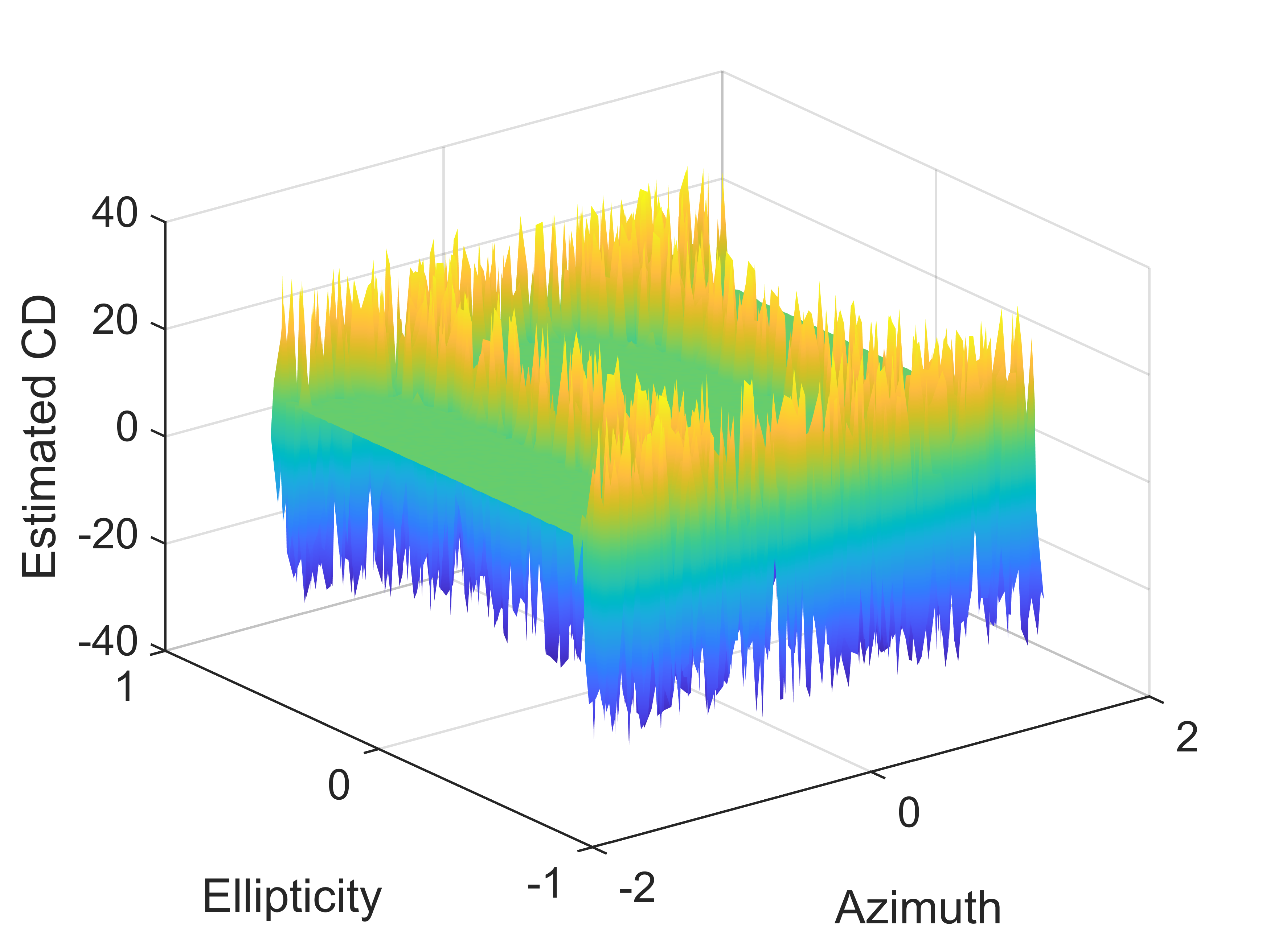
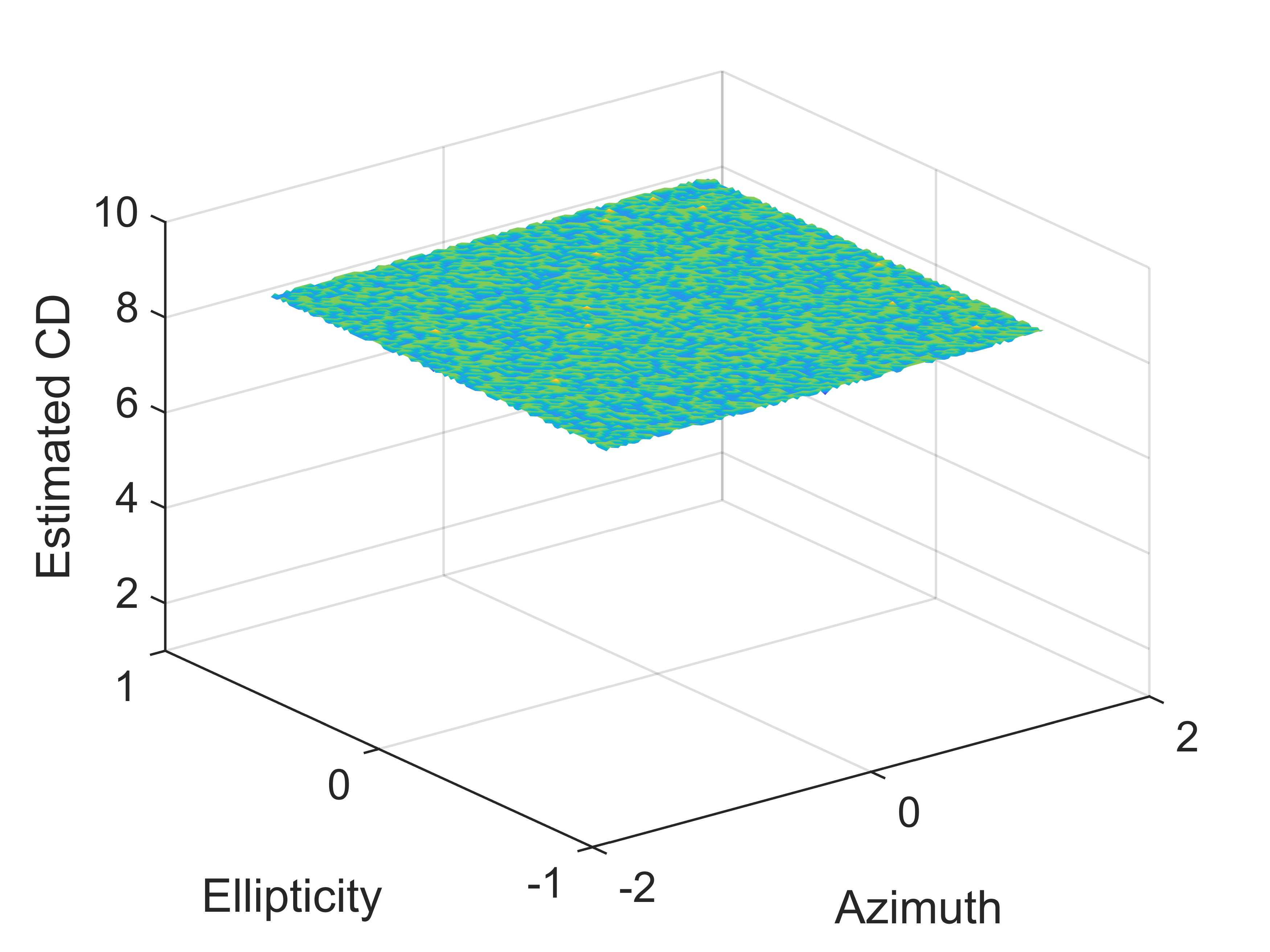
Figure 4: Simulation results of CD estimation (ns/nm) based on the estimator given by (a) equ. (30) and (b) equ. (32), respectively. Simulation parameters are the same as those for Fig. 3 with fiber CD of $8.5$ ns/nm.

III-C Case of Large DGD

When the DGD is large, we first note that $\operatorname{trace}(\bar{P^{\prime}})$ has a clear dependence on the PMD [cf. (18)]. But the quantity

$$\operatorname{trace}(\bar{P^{\prime}}U^{H})=\operatorname{trace}(UV\bar{P}V^{H}U^{H})\approx 2e^{-j\phi_{0}}$$ (21)

is an exact timing phase detector independent of PMD, provided we know $U$. However, there is no obvious way to estimate the true $U$ without being affected by the timing phase [cf. (18)]. On the other hand, it is remarkable that despite the potentially time-varying phase term $e^{-j\phi_{0}}$, both DGD and PSP can be estimated from the matrix $\bar{P^{\prime}}$. Since $U$ has two eigenvalues $\rho=e^{\pm j\pi\alpha\tau_{\text{DGD}}}$, the DGD can be estimated from the two eigenvalues of $\bar{P^{\prime}}$, the estimate of $U$, via

$$\widehat{\tau_{\text{DGD}}}=|\arg\{\rho_{1}\rho_{2}^{*}\}|/(2\pi\alpha)$$ (22)

with a wrapped range from zero to half symbol duration due to the multi-valued argument function $\arg(\cdot)$ and the PSP vector can be estimated via

$$\widehat{p_{i}}=k\cdot\operatorname{Im}\left[\operatorname{trace}\left(\sigma_{i}\bar{P^{\prime}}\right)\cdot\operatorname{trace}(\bar{P^{\prime}})^{H}\right]$$ (23)

where $i=1,2,3$ and $k$ is a constant such that the estimated vector is normalized. It is easy to verify that $\widehat{p_{i}}$ has a dependence $\sin(2\pi\alpha\tau_{\text{DGD}})$ on the true DGD $\tau_{\text{DGD}}$. We can combine (22) and (23) to form an estimate of $U$ that is independent of timing phase, i.e.,

$$\hat{U}=\cos(\pi\alpha\widehat{\tau_{\text{DGD}}})I-j\sin(\pi\alpha\widehat{\tau_{\text{DGD}}})[\vec{p}\cdot\vec{\sigma}]\,.$$ (24)

Note that the sign of $\hat{U}$ depends on both $\tau_{\text{DGD}}$ and $\widehat{\tau_{\text{DGD}}}$ and cannot be determined based on $\widehat{\tau_{\text{DGD}}}$ alone. This sign ambiguity prohibits the use of $\operatorname{trace}(\bar{P^{\prime}}\hat{U}^{H})$ as a timing phase detector for an arbitrary DGD. It does work when the true DGD is strictly less than half of the symbol duration.

III-D All DGD Cases

On the other hand, we see that the determinant of $P^{\prime}$

$$\operatorname{det}(\bar{P^{\prime}})=\operatorname{det}(UV\bar{P}V^{H})=e^{-2j\phi_{0}}$$ (25)

is PMD independent. Its imaginary part, $-\operatorname{Im}\{\operatorname{det}(\bar{P^{\prime}})\}$, is a timing error detector with characteristic curves shown in Fig. 3(d). It has two positive zero-crossings and hence two locking points. Depending on the initial state, the timing recovery loop may lock to one of the two points. For instance, when the initial timing phase is $>0.25$ or $<-0.25$ unit interval (i.e., one symbol), it locks to the symbol edges. This property combined with the varying polarization mixing due to PMD would not be a prominent problem if fractional-spaced channel equalizer is used after the timing unit. Otherwise, it might affect the DSP performance when the symbol-spaced equalizer is used afterwards. However, this is a common problem for all TEDs considering the fact that the concept of optimal sampling phase is complicated by the combined effect of locking point and PMD. Note that the TED based on (25) is completely transparent to the first-order PMD and polarization rotation. It is indeed slightly more complex than the simple trace operation given by (20). In light of (9) and (25), we could also extract directly a clock tone, independent of PMD, at the baudrate from the spectrum

$$F=F_{xx}F_{yy}-F_{xy}F_{yx}\,,$$ (26)

where $F_{xx}$ is the fast Fourier transform (FFT) of $xx^{*}$, $F_{xy}$ is the FFT of $xy^{*}$, etc., and $x$, $y$ are signals from two polarizations after CD compensation.

III-E Adaptive Method

First introduced in [9] and furthered studied in [14], the linear combination of the elements of matrix $\bar{P^{\prime}}$ seems a feasible way to deal with the PMD effect. Consider the quantity

$$q=P^{\prime}_{xx}+e^{j\phi_{xy}}P^{\prime}_{xy}+e^{j\phi_{yx}}P^{\prime}_{yx}+e^{j\phi_{yy}}P^{\prime}_{yy}\,,$$ (27)

the imaginary part of which, $-\operatorname{Im}\{q\}$, can be used as the timing error detector if the phase vector $[\phi_{1},\phi_{2},\phi_{3}]$ is adapted jointly with the timing loop such that the above quantity converges to a purely real-valued number when the joint loop is locked. The update at time instance $k$ is written as

$$\phi^{k}_{l}=\phi^{k-1}_{l}-\mu\operatorname{Im}(e^{j\phi^{k-1}_{l}}P^{\prime}_{l}),\quad l=xy,yx,yy$$ (28)

It effectively treats the four entries of the SCF matrix (17) as independent timing phase detectors. Note that unlike previous timing error detectors, the timing loop does not lock to the true phase $\phi_{0}$ via the adaptive method but to the phase of $P^{\prime}_{xx}$, which is $\phi_{0}$ plus the phase of the first element of $U$. This adds noise to the timing loop considering $U$ is an erratic effect in practice.

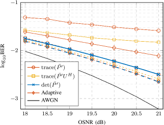
Figure 5: Simulation results of a $32$ GBaud PDM-16QAM system bit error rate (BER) versus optical signal-to-noise ratio (OSNR) when various timing recovery algorithms are implemented. The solid lines are for the cases when symbol-spaced LMS equalizer is used. Whereas the dashed lines are when fractional-spaced equalizer is used.

IV CD Effect

It is well-known that the chromatic dispersion of optical fiber incurs a quadratic phase change over the entire signal spectrum. The frequency response of CD is given by

$$H=\exp(jKf^{2})$$ (29)

with $K=\pi\lambda^{2}DL/c$, where $\lambda$ is the wavelength, $D$ dispersion coefficient, $L$ fiber length, and $c$ the speed of light. According to (5), the CD effect results in a linear phase change in the SCF with the change rate over frequency equal to $2K\alpha$. The linear phase suppresses the timing error upon integration in (8). The solution to restore the timing sensitivity is to estimate the CD value from the slope of phase [19] and then remove the linear phase from SCF during integration [14]. On the other hand, the linear phase in SCF is equivalent to a constant time shift in CAF due to their Fourier relation. The CAF is a pulse-like function and hence the time shift can be identified by peak searching of $|R_{x}^{\alpha}|^{2}$. Namely,

$$\tau_{\text{CD}}=\arg\max|R_{xx}^{\alpha}(\tau)|^{2}\,.$$ (30)

Note that the CAF can be computed efficiently by taking the inverse Fourier transform of SCF. The CAF peak location can also distinguish the sign of CD, provided the time shift due to CD is no larger than half of the CAF duration. Moreover, it is easy to verify that the length of CAF determines the maximum range of CD estimate not the resolution. A higher resolution of CD estimation can only be obtained by a higher sampling rate of the signal. After obtaining the delay of CAF peak $\tau_{\text{CD}}$, the timing error can be detected simply by using $\operatorname{Im}R_{x}^{\alpha}(\tau_{\text{CD}})$ [12].

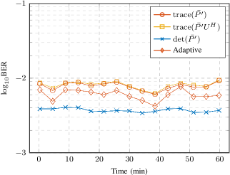
Figure 6: Filed-test results of a $1$-hour BER on a $32$ GBaud PDM-16QAM coherent system over the $153$ km optical cable. A $2000$ rad/s polarization scrambling at the fiber input is utilized. The DSP setup is the same as that used for simulations with one sample per symbol, except that the LMS channel equalizer has $11$ taps for symbol-spaced configurations. The block length for performing various TEDs is 512 symbols. Each BER result is obtained based on 4 million bits.

Assuming little dependence on polarization, the CD effect is modeled as a common term in both CAF and SCF. In particular, it causes a time shift in the CAF matrix and a linear phase change in the SCF matrix in (10). The development in the last section is similar in the presence of CD, except that the matrix relation in (11) should be modified as

$$C(\tau_{\text{CD}})=\int S(f)e^{j2\pi f\tau_{\text{CD}}}\,df=Ae^{-j2\pi\alpha\tau_{g}}I$$ (31)

and in the presence of first-order PMD, $\hat{C}(\tau_{\text{CD}})\approx e^{-j\phi_{0}}U$ is an PMD matrix estimate insensitive to both CD and polarization rotation. Note that the form of $U$ given in (14) clearly suggests that the search of CAF peak is affected by the PMD. Namely, using $|R_{xx}^{\alpha}|^{2}$ or $|R_{yy}^{\alpha}|^{2}$ or any linear combination of them will loss sensitivity at $\tau_{\text{CD}}$ when $a$, the first element of $U$, is approaching zero. However, the PMD effect is irrelevant if we use $|R_{xx}^{\alpha}|^{2}+|R_{yx}^{\alpha}|^{2}$, because $|a|^{2}+|b|^{2}=1$. Namely,

$$\tau_{\text{CD}}=\arg\max\big{\{}|R_{xx}^{\alpha}(\tau)|^{2}+|R_{yx}^{\alpha}(\tau)|^{2}\big{\}}\,.$$ (32)

Therefore, we find a way to estimate the CD value completely independent of polarization rotation, PMD and timing phase. After that, the matrix $\hat{C}(\tau_{\text{CD}})$ can be worked with to detect timing error according to the methods introduced in the last section.

Figure 4 shows the CD estimation results when (30) and (32) are used respectively. A half-symbol DGD and all possible PSP states are considered in the simulation. The results confirm that (32) is insensitive to the PMD. The previous results suggest that the timing recovery could be performed without actual CD and/or PMD compensation, which could be useful in certain practical use cases.

V Higher-Order Cyclostationarity

The studies presented in previous sections are based on second-order cyclostationarity of common signals, which is however not suitable for the analysis of severely filtered signal with no excess bandwidth. Fortunately, the statistics of higher-order cyclostationarity can be exploited for proper timing phase detection in such cases (to be published). Although not well recognized by the research community, most of the proposed timing phase detectors for such signals, such as those listed in Table 1, are based on the fourth-order cyclostationarity. However, the CD and PMD effect on this class of timing phase detector remains unknown. It is not a straightforward task of extending the analysis in this paper to higher order statistics. It is however clear that efforts are required to study the spectral properties of higher-order correlation, which certainly is an interesting direction for future research.

TABLE I: Common fourth-order timing recovery algorithms

Ref.	Algorithm
[20]	${\sum}_{k=1}^{m}(x_{2k}x_{2k}^{*}+y_{2k}y_{2k}^{*})[(x_{2k+1}x_{2k+1}^{*}+y_{2k+1}y_{2k+1}^{*})-(x_{2k-1}x_{2k-1}^{*}+y_{2k-1}y_{2k-1}^{*})]$
[21]	${\sum}_{k=1}^{m}x_{2k}x_{2k+1}^{*}(x_{2k+1}x_{2k+2}^{*}-x_{2k-1}x_{2k}^{*})+y_{2k}y_{2k+1}^{*}(y_{2k+1}y_{2k+2}^{*}-y_{2k-1}y_{2k}^{*})$
[22]	${\sum}_{k=1}^{m}x_{k}x^{*}_{k+1}[x_{k}x^{*}_{k}-x_{k+1}x^{*}_{k+1})]$
[23]	$E\left\{\text{Re}\left[(x_{-1}^{*}+x_{0}^{*})(x_{0}+x_{1})((x_{-2}+x_{-1})(x_{-1}^{*}+x_{0}^{*})-(x_{0}+x_{1})(x_{1}^{*}+x_{2}^{*}))\right]\right\}$

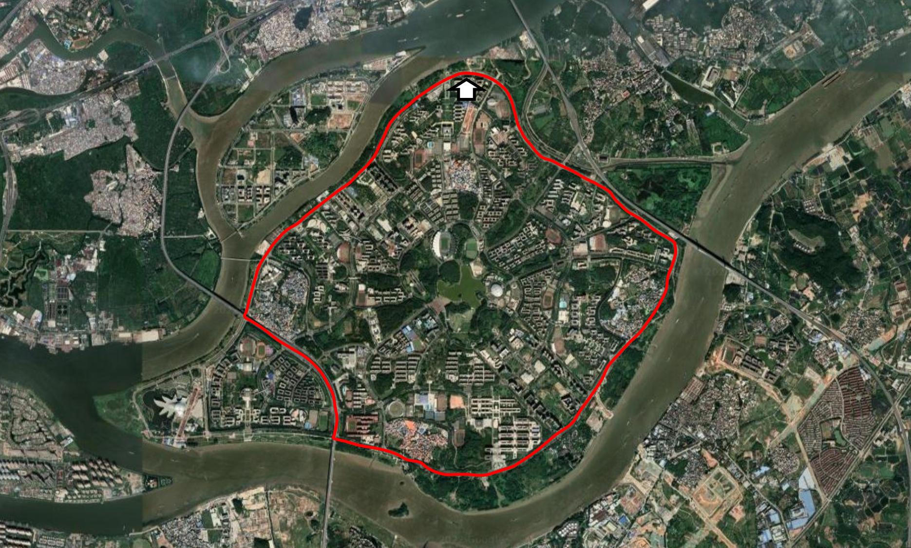
Figure 7: The subterranean optical cable containing several single mode fibers (SMF) used for the field tests. The arrow indicates the location of our lab and also the two ends of the cable. The optical signal circulates the cable 9 times, one SMF at a time, and forms the 153 km optical link for the test.

VI Numerical Simulation

We perform numerical simulations of a 32 GBaud PDM-16QAM system with 100 km standard single mode fiber (SSMF) transmission. The laser linewidth is 100 kHz. The laser frequency offset is considered negligible or has been compensated prior to the timing recovery. The fiber SOP rotation speed is 50,000 rad/s. The jitter effect of ADC is simulated as a sinusoidal model with a 30 kHz frequency and $0.6T_{0}$ peak deviation of sampling instance. The fiber DGD also varies from 6 ps to 16 ps in a sinusoidal manner with a frequency of 260 kHz. It provides a critical situation for testing the performance of various TED algorithms. The DSP chain includes in sequence CD estimation, CD compensation, timing recovery, least mean squares (LMS) dual-polarization channel equalization with embedded phase lock loop (PLL) for carrier phase recovery. When the LMS equalizer works in the symbol spaced mode, the performance of timing recovery becomes prominent. The simulation results are shown in Fig. 5. Note that the LMS equalizer has 7 and 13 taps respectively for the symbol-spaced and fractional-spaced mode for fair comparison. The TED $-\operatorname{Im}\{\operatorname{det}(\bar{P^{\prime}})\}$ gives the best performance for all cases but the differences are less significant when fractional-spaced equalizer is utilized [24].

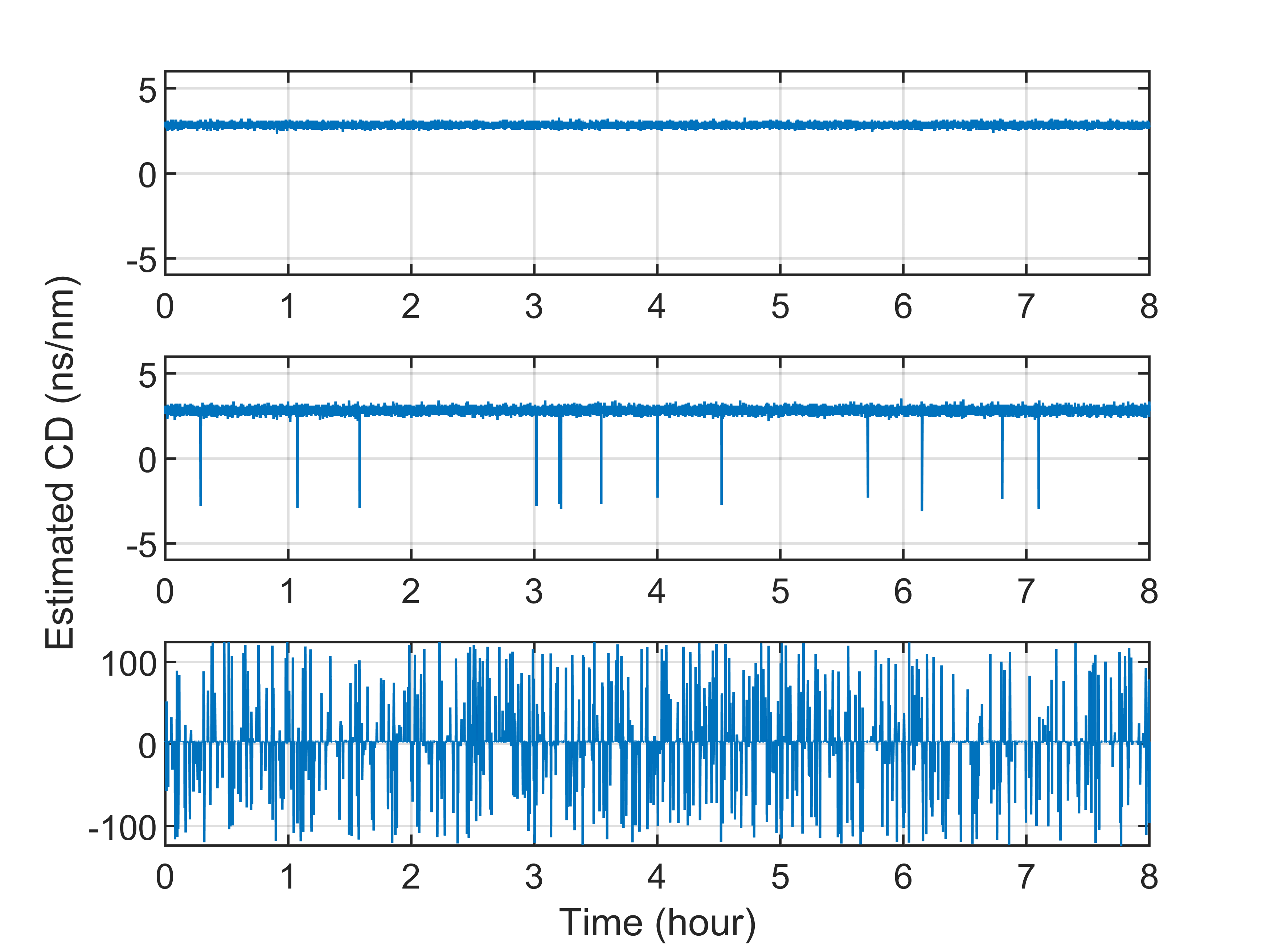
Figure 8: Filed-test results of an $8$-hour CD estimation on a $32$ GBaud PDM-16QAM coherent system over the $153$ km optical cable. Subfigure from top to bottom: (a) estimator (32) with $2000$ rad/s polarization scrambling at the fiber input, (b) estimator (30) without polarization scrambling, and (c) estimator (30) with $2000$ rad/s polarization scrambling at the fiber input. Each measurement is performed by evaluating (30) and (32) based on a data block containing 2048 symbols.

VII Field Test

We exploit the field optical fiber cable as illustrated in Fig. 7. It has several standard single mode fibers (SMF) which can be interconnected at the cable ends so that the signals circulate inside the fiber loop. The total length of the fiber loop is measured to be 153 km consisting 9 interconnected SMFs. An optical amplifier with 20 dB gain is used at the input to the 3rd, 6th, and 8th SMF, respectively. A 32 GBaud PDM-16QAM signal carried by a 1550 nm laser light is launched with 0 dBm power into the fiber loop and coherently detected at the receiver end. We use a 80 GSa/s oscilloscope to sample the detected signal and run signal processing offline. Fig. 8 shows the long term CD estimation results when (30) and (32) are used. It confirms the stability of (32) by comparing Fig. 8(a) and (c) where polarization scrambling is enabled at the fiber input. The maximal SOP speed is limited to 2000 rad/s by the device in our lab. Note that without scrambling, the natural condition of the field cable is fairly stable as shown in Fig. 8(b). A 1-hour BER test is performed and the results are shown in Fig. 6. It is again confirmed that the TED $-\operatorname{Im}\{\operatorname{det}(\bar{P^{\prime}})\}$ gives the best performance for all cases.

VIII Conclusion

We have studied in detail the CD and PMD effect on the second-order cyclostationarity-based timing recovery commonly used in optical coherent receivers. We have proposed for $\alpha=1/T_{0}$ the estimator of CD

$$\widehat{DL}=\frac{cT_{0}}{\lambda^{2}}\cdot\tau_{\text{CD}}$$ (33)

where $\tau_{\text{CD}}=\arg\max\big{\{}|R_{xx}^{\alpha}(\tau)|^{2}+|R_{yx}^{\alpha}(\tau)|^{2}\big{\}}$, the estimator of PMD matrix

$$\widehat{U_{T}}=\hat{C}(\tau_{\text{CD}})\approx e^{-j2\pi\alpha\tau_{g}}U\,,$$ (34)

where $\tau_{g}$ is the group delay, the DGD estimator

$$\widehat{\tau_{\text{DGD}}}=\big{|}\arg\{\rho_{1}\rho_{2}^{*}\}\big{|}/(2\pi\alpha)\,,$$ (35)

where $\rho_{1}$ and $\rho_{2}$ are the two eigenvalues of $\widehat{U_{T}}$, and the PSP estimator $\vec{p}=[\widehat{p_{1}},\widehat{p_{2}},\widehat{p_{3}}]$ with

$$\widehat{p_{i}}=k\cdot\operatorname{Im}\left[\operatorname{trace}\left(\sigma_{i}\widehat{U_{T}}\right)\cdot\operatorname{trace}(\widehat{U_{T}})^{H}\right]\,,$$ (36)

where $\sigma_{i}$ is one of the three Pauli matrices. The CD estimator is insensitive to polarization rotation, PMD and timing error. The PMD matrix estimator is immune to polarization rotation but affected by timing error. The DGD and PSP estimators are not affected by polarization rotation and timing error, but are valid only when the true DGD is less than $T_{0}/2$.

Based on the estimators, we have proposed timing error detectors for the case when the DGD is negligible

$$e_{T}=\operatorname{Im}\operatorname{trace}(\widehat{U_{T}})\,,$$ (37)

and for the case when DGD is smaller than $T_{0}/2$

$$e_{T}=\operatorname{Im}\operatorname{trace}(\widehat{U_{T}}\hat{U}^{H})\,,$$ (38)

where $\hat{U}=\cos(\pi\alpha\widehat{\tau_{\text{DGD}}})I-j\sin(\pi\alpha\widehat{\tau_{\text{DGD}}})[\vec{p}\cdot\vec{\sigma}]$ , and for larger DGD to use the adaptive combination of $R_{xx}^{\alpha}$, $R_{xy}^{\alpha}$, and $R_{yy}^{\alpha}$, and finally for all channel conditions

$$e_{T}=\operatorname{det}(\widehat{U_{T}})\,.$$ (39)

Both numerical simulations and field tests confirm that (39) is a universal timing phase detector regardless of the CD and PMD condition when the matrix is given by (34).

References

- [1] S. J. Savory, “Digital coherent optical receivers: Algorithms and subsystems,” IEEE Journal of Selected Topics in Quantum Electronics, vol. 16, no. 5, pp. 1164–1179, 2010.
- [2] M. S. Faruk and S. J. Savory, “Digital signal processing for coherent transceivers employing multilevel formats,” Journal of Lightwave Technology, vol. 35, no. 5, pp. 1125–1141, 2017.
- [3] K. Kikuchi, “Fundamentals of coherent optical fiber communications,” Journal of Lightwave Technology, vol. 34, no. 1, pp. 157–179, 2015.
- [4] X. Zhou, “Efficient clock and carrier recovery algorithms for single-carrier coherent optical systems: A systematic review on challenges and recent progress,” IEEE Signal Processing Magazine, vol. 31, no. 2, pp. 35–45, 2014.
- [5] D. Godard, “Passband timing recovery in an all-digital modem receiver,” IEEE Transactions on Communications, vol. 26, no. 5, pp. 517–523, 1978.
- [6] F. Gardner, “A BPSK/QPSK timing-error detector for sampled receivers,” IEEE Transactions on Communications, vol. 34, no. 5, pp. 423–429, 1986.
- [7] M. Oerder and H. Meyr, “Digital filter and square timing recovery,” IEEE Transactions on Communications, vol. 36, no. 5, pp. 605–612, 1988.
- [8] J. C. M. Diniz, F. Da Ros, and D. Zibar, “Clock recovery challenges in dsp-based coherent single-mode and multi-mode optical systems,” Future Internet, vol. 10, no. 7, p. 59, 2018.
- [9] F. Hauske, N. Stojanovic, C. Xie, and M. Chen, “Impact of optical channel distortions to digital timing recovery in digital coherent transmission systems,” in 2010 12th International Conference on Transparent Optical Networks. IEEE, 2010, pp. 1–4.
- [10] D. Zibar, J. C. R. de Olivera, V. B. Ribeiro, A. Paradisi, J. C. Diniz, K. J. Larsen, and I. T. Monroy, “Experimental investigation and digital compensation of DGD for 112 Gb/s PDM-QPSK clock recovery,” Optics Express, vol. 19, no. 26, pp. B429–B439, 2011.
- [11] L. Huang, D. Wang, A. P. T. Lau, C. Lu, and S. He, “Performance analysis of blind timing phase estimators for digital coherent receivers,” Optics Express, vol. 22, no. 6, pp. 6749–6763, 2014.
- [12] D. Wang, Z. Su, H. Jiang, G. Liang, Q. Zhan, and Z. Li, “Modified square timing error detector with large chromatic dispersion tolerance for optical coherent receivers,” Optics Express, vol. 29, no. 13, pp. 19 759–19 766, 2021.
- [13] C. Malouin, P. Thomas, B. Zhang, J. O’Neil, and T. Schmidt, “Natural expression of the best-match search Godard clock-tone algorithm for blind chromatic dispersion estimation in digital coherent receivers,” in Signal Processing in Photonic Communications. Optica Publishing Group, 2012, pp. SpTh2B–4.
- [14] H. Sun and K.-T. Wu, “A novel dispersion and PMD tolerant clock phase detector for coherent transmission systems,” in 2011 Optical Fiber Communication Conference and Exposition and the National Fiber Optic Engineers Conference. IEEE, 2011, pp. 1–3.
- [15] N. Stojanović, C. Xie, Y. Zhao, B. Mao, and N. G. Gonzalez, “A circuit enabling clock extraction in coherent receivers,” in 2012 38th European Conference and Exhibition on Optical Communications. IEEE, 2012, pp. 1–3.
- [16] V. N. Rozental, B. Corcoran, and A. J. Lowery, “Correlation-based polarization demultiplexing for clock recovery in coherent optical receivers,” in Optical Fiber Communication Conference. Optica Publishing Group, 2017, pp. W2A–47.
- [17] H. Sun, “Clock and carrier recovery for coherent receivers,” in 2015 European Conference on Optical Communication (ECOC). IEEE, 2015, pp. 1–3.
- [18] W. Gardner, “The role of spectral correlation in design and performance analysis of synchronizers,” IEEE Transactions on Communications, vol. 34, no. 11, pp. 1089–1095, 1986.
- [19] M. Ionescu, M. Sato, and B. Thomsen, “Cyclostationarity-based joint monitoring of symbol-rate, frequency offset, cd and osnr for nyquist wdm superchannels,” Optics Express, vol. 23, no. 20, pp. 25 762–25 772, 2015.
- [20] M. Yan, Z. Tao, L. Dou, L. Li, Y. Zhao, T. Hoshida, and J. C. Rasmussen, “Digital clock recovery algorithm for Nyquist signal,” in 2013 Optical Fiber Communication Conference and Exposition and the National Fiber Optic Engineers Conference (OFC/NFOEC). IEEE, 2013, pp. 1–3.
- [21] N. Stojanovic, B. Mao, and Y. Zhao, “Digital phase detector for Nyquist and faster than Nyquist systems,” IEEE Communications Letters, vol. 18, no. 3, pp. 511–514, 2014.
- [22] M. Moeneclaey and T. Batsele, “Carrier-independent NDA symbol synchronization for M-PSK, operating at only one sample per symbol,” in [Proceedings] GLOBECOM’90: IEEE Global Telecommunications Conference and Exhibition. IEEE, 1990, pp. 594–598.
- [23] N. Stojanovic, F. N. Hauske, C. Xie, and M. Chen, “Clock recovery in coherent optical receivers,” in Photonic Networks, 12. ITG Symposium. VDE, 2011, pp. 1–4.
- [24] K. Kikuchi, “Clock recovering characteristics of adaptive finite-impulse-response filters in digital coherent optical receivers,” Optics Express, vol. 19, no. 6, pp. 5611–5619, 2011.