Determining a Points Configuration on the Line from a Subset of the Pairwise Distances
Abstract
We investigate rigidity-type problems on the real line and the circle in the non-generic setting. Specifically, we consider the problem of uniquely determining the positions of distinct points given a set of mutual distances . We establish an extremal result: if , then the positions of a large subset , where large means , can be uniquely determined up to isometry. As a main ingredient in the proof, which may be of independent interest, we show that dense graphs for which every two non-adjacent vertices have only a few common neighbours must have large cliques.
Furthermore, we examine the problem of reconstructing from a random distance set . We establish that if the distance between each pair of points is known independently with probability for some universal constant , then can be reconstructed from the distances with high probability. We provide a randomized algorithm with linear expected running time that returns the correct embedding of to the line with high probability.
Since we posted a preliminary version of the paper on arxiv, follow-up works have improved upon our results in the random setting. Girão, Illingworth, Michel, Powierski, and Scott proved a hitting time result for the first moment at which an time at which one can reconstruct when is revealed using the Erdős–Rényi evolution, our extremal result lies in the heart of their argument. Montgomery, Nenadov and Szabó resolved a conjecture we posed in a previous version and proved that w.h.p a graph sampled from the Erdős–Rényi evolution becomes globally rigid in at the moment it’s minimum degree is .
1 Introduction
Let be a set of distinct points in a metric space. Given a subset of pairwise distances of , we inquire whether all other distances in can be uniquely determined. In with , it is easy to construct examples where all distances are known except one distance, yet this distance cannot be deduced from the others. In order to say something meaningful on rigidity a popular line of work is to assume general position, e.g. that the points are in generic position, meaning that all the coordinates of elements of are algebraically independent over . In that case, it is known to be a property of the graph that does not depend on the distances of elements in .
In , it is well known that if the points are in generic position, then all distances are determined by if and only if is -connected, as shown in [7]. However, when the points are not in generic position, it is easy to build an example with points and given distances in which -connectivity is no longer sufficient.
We study rigidity without assuming general position but only assuming the weaker assumption that are different points, and show that when the points are in the set of pairwise distances known does carry meaningful information.
A graph is said to be globally rigid in if, for any injective map , the distance between for determines uniquely the distances of all pairs. A characterization of globally rigid graphs in in the injective setting was obtained by [4] (Theorem 2.4). They established that certain edge colorings of the graph serve as witnesses for the graph being not globally rigid in . Furthermore, they showed that recognizing whether a graph is globally rigid in is an NP-complete problem.
To conclude the preceding discussion, we emphasize that although there exists a significant amount of research on globally rigid graphs, it focuses to the generic setting, where the embedding function satisfies a strong condition of being generic. In contrast, the results presented in this paper apply under a much weaker assumption, namely that is injective.
We consider points in either or , which may not necessarily be in generic position. We first examine an arbitrary distance sets . We prove that every dense enough graph contains a dense globally rigid subgraph.
Theorem 1
Let be a subset of either or of size and let be the set of given distances. If , then there exists s.t. all distances between elements of can be deduced from and .
We prove the following stronger claim. Consider a set of objects whose explicit representation is unknown. Assume we have knowledge of the result of a certain function for some pairs of elements in and the objective is to reconstruct some subset of the elements of from these measurements. That is, we would like to determine the valuations of all the pairs in some subset of , with large.
We say that a function is -locally determined if can be determined from the values of for different elements in . Let be the set of pairs for which the valuations are known, then:
Theorem 2
Let be a set of elements, and let be a -locally determined function with a measurement set . If , there exists a subset of size for which all the measurments on are determined from .
To prove the bound given in Theorem 1, we demonstrate that distances in and are and locally-determined, respectively, and then apply Theorem 2.
We also study what can be deduced from a random , and show that the situation differs significantly. In this case, we show that if the distance between each pair of elements in is known with probability , independently, and for a large enough constant , then there is a linear expected running time algorithm that returns a correct embedding to the line with high probability.
Theorem 3
Let be distinct points in . There exists a constant such that when each pairwise distance is known with probability , independently, then all other distances can be deduced from with high probability.
The main ingredient in the proof of the claim above is proving a sharp threshold for having a monotone path from to in an Erdős–Rényi random graph with vertex set . Specifically, we prove that there is a sharp threshold for the existence of such a path at .
Remarks on advancements after first arxiv version
Since the first publication Girão, Illingworth, Michel, Powierski, and Scott [5] proved a hitting time result for the first moment at which an time at which one can reconstruct when is revealed using the Erdős–Rényi evolution. They proved that one can reconstruct at the moment where the minimum degree of the graph is , In particular they proved Theorem 3 holds with any constant . Their proofs relies heavily on Theorem 1.
The work of Barnes, Petr, Portier, Randall Shaw and Sergeev [2] made progress on a question of Girão, Illingworth, Michel, Powierski, and Scott [5] and gave the first non trivial bounds on the required density of a random set of distances, such that given points in , one can reconstruct all distances between of the points from the distances in .
2 Reconstructing a subset of or
We start by showing that the distance functions in and are locally determined respectively.
Claim 4
Given , and common neighbours in one can determine the distance from their distances to the common neighbours.
Proof.
Consider the functions . As attains maximum outside the segment , and attains any other value at most twice inside . Let be three common neighbours of . If all are equal then . Otherwise, pick the element with minimal value among , w.l.o.g it is , this implies lies inside and hence can be determined. ∎
In five common neighbors are enough.
Claim 5
Given , and common neighbours in one can determine the distance from their distances to the common neighbours.
Proof.
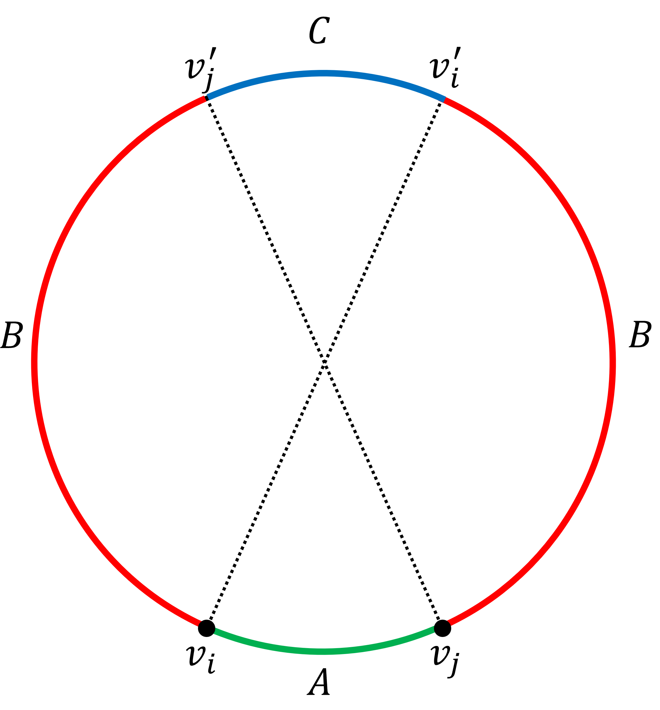
Let be common neighbors of . Consider the 3 regions in Figure 1, and again consider the function . If has the same value for all then necessarily this is the distance from to and all points are in region .
Otherwise w.l.o.g we may assume that attains the minimum over all . This means that is not in the region . Hence if then is at region and , and if then is at region and . ∎
2.1 Proof of Theorem 2
Let be the graph of given measurements. Define the graph of determined valuations, which contains as edges all possible pairs that can be determined from by the locality of . Let denote the set of neighbors of in . Since contains all possible pairs that can be determined it means that . Denote by the size of a maximum independent set of and by the size of the maximum clique in .
Therefore the following implies Theorem 2:
Theorem 6
Let be a graph on vertices, such that .
If then .
We remind the following standard lemma:
Lemma 7
Let be a graph of average degree . There exists an induced subgraph with minimal degree satisfying
Proof.
Iteratively delete from vertices of degree smaller than . Each deletion only increases the average degree, so this process must terminate and the final set of vertices induce the desired subgraph. ∎
Consequently, from now we assume that has minimal degree with . To ease the notation we refer to as .
To bound the size of the maximal independent set of . We need the following result due to Corrádi, whose proof appears in [8] (Lemma 2.1):
Lemma 8
Let be subsets of a set , each of size with then:
We now bound the size of the maximal independent set in by applying Corrádi’s Lemma:
Claim 9
Let be a graph on vertices such that all non-neighbours satisfy . If the minimal degree of satisfies then the size of a maximum independent set in satisfies
Proof.
Denote the elements of the maximum independent set by . By Lemma 8 applied to :
Rearranging this inequality yields:
∎
Proof of Theorem 6.
We assume that the graph has minimal degree . Let be any independent set of maximum size. Since by assumption one can apply 9 to obtain that . Define to be the set of elements that has only as a neighbour in . Formally , i.e. it is the set of elements in for which is their unique neighbor from the set . The following observation is the heart of the argument:
Observation 10
Each form a clique in .
The observation follows by noticing that if are not adjacent then is an independent set. (see Figure 2).

Right: is a clique since replacing with non-adjacent increases the size of a maximum independent set.
Thus it follows that:
| (1) |
To estimate , first estimate by using Bonferroni’s inequality and get:
Observe that the set consists of exactly the elements in that do not appear in any for all , therefore:
Plugging this into Equation 1 and using 9 we get since :
∎
Notice that the clique size achieved by Theorem 6 is asymptotically tight by considering disjoint union of cliques of size roughly . We note that the requirement cannot be improved as well.
Claim 11
For every , there are graphs satisfying the assumptions of Theorem 6, with and .
Proof.
Let be a -free graph with edges, e.g. one may take the well-known ”lines vs planes” graph of the incidences of lines and planes of for a prime . Denote by it’s vertex set, and let denote the size of . Observe that by being -free for any .
If we consider the graph , obtained by replacing each vertex of by a -clique and each edge of by all possible edges between the new cliques, then we obtain with and , moreover every two vertices in this graph has common neighbors, hence this graph satisfies the conditions of this claim as:
And has maximum clique of size as needed. ∎
Reconstructing points on the 3-Regular tree requires distances
It is natural to ask whether we can find analogs of Theorem 1 for subsets of metric spaces that are not or . We now consider the 3-regular tree with the graph metric. We give an example of a set of size for which we cannot fully reconstruct a subset of size 3.
Consider the infinite binary tree, and associate each vertex of distance from some root by a length string over . Consider the two subsets of vertices of level , and . Notice that every two vertices of are at distance at most , and every two vertices of are at distance at least .
For the -regular tree, notice that for an edge the graph is isomorphic to two copies of the infinite binary tree. Define the set to be taking two copies of in each infinite binary tree in . If the set of distances known, , is the set of all distances between vertices in the different binary trees, then all distances in is and we cannot distinguish which have all other distances different, see Figure 3. We also note this construction is tight since we constructed points and known distances for which no points can be reconstructed and by Mantel’s theorem adding one more pair to yield a triangle in the distance graph.

Sparse globally rigid graphs in
4 has also the following application to injective global rigidity. A graph is globally rigid in if given an injective map all the distances of determine all other distances uniquely (or equivalently, determine up to isometry). The proof of Theorem 6 gives that dense enough graphs contain large globally rigid subgraphs. We note that 4 implies that there are infinitely many globally rigid graphs with average degree at most .
To see this, first notice that if is globally rigid in then adding a new vertex along with two edges to vertices of yields a new graph that is also rigid. Given a graph , define to be a graph with and , i.e. each edge is replace by 3 paths of length two. Note that for every , thus by 4 all the distances of vertices that correspond to the original edges of can be deduced from . This means that is rigid since all distances of can be recovered from it, and the vertices of all contain two edges that connect to . Note that if then . Hence one can construct an infinite family of graphs by a clique of size 3 and take . This infinite family has average degree since the sequence is the sequence , which converges to .
We note that the average degree of a globally rigid graph must be substantially larger than what’s possible in the generic setting:
Proposition 12
Any globally rigid graph with at least vertices has average degree of at least .
Proof.
Let be a connected graph and let be the set of vertices of degree . Observe that if is globally rigid in then must be an independent set. Indeed, for assuming they must lie on a path for since is connected and . Let be an injective map and consider:
Notice that and induce the same distances on . As is arbitrary, then for some both and are injective and therefore is not globally rigid.
Therefore is an independent set. Furthermore, it is clear that a globally rigid graph must have minimum degree . Now consider the size of . If then and therefore .
If then as needed. ∎
3 Reconstruction from Random
We now consider the case of a fixed set of points and a set of pairs sampled randomly, i.e. for each pair we know the distance between point and point with probability . We show that for with being some universal constant it is possible to reconstruct w.h.p. We also show that at this , there is a randomized algorithm with expected running time linear in that returns the correct location of the points of up to isometry w.h.p.
Before giving the full proof we sketch the strategy of the proof. Let be the random pairs samples, and is a Erdős–Rényi random graph.
At the probability specified above we do not expect to vertices to have common neighbors as this event occurs at . Since the graph at our range of looks locally like a tree and the local structure is not rigid. Denote by the set of all walks between in the graph . We can define an estimate of the distance between two nodes to be where is a walk from to , i.e. it is the distance in the graph metric between in the graph . It is clear that . We will show that for far enough points (with points between them in the order induced by ) have w.h.p.
The estimate , even though correctly estimates far enough points, is usually incorrect for close points, see Figure 4. To bypass this, we observe that if is incorrect, then with many , the three numbers do not satisfy the triangle equality (w.h.p). We also show the other direction, that is: if is correct, then with many , the terms satisfy the triangle inequality. Combining these we get that we can find (w.h.p) the correct efficiently, by checking triangle equalities.

Therefore, let be points in and assume and let be an Erdős–Rényi random graph on vertex set where we associate the vertex with , then by the preceding discussion we’d like to understand when is which is exactly when there is a monotone path from to in 111where by monotone we mean the sequence of vertex indices along the path is monotone. We show that there is a sharp threshold at for the existence of a monotone path from to in a random graph, that is:
Theorem 13
Let be a random graph with vertex set , then for any :
-
•
(Subcritical) If then w.h.p there is no monotone path from to .
-
•
(Supercritical) If then w.h.p there is a monotone path from to .
Remark 14
In fact, we show in the supercritical regime that for each the corresponding events happen with probability where is some constant depending on and .
By the remark above we have:
Corollary 15
There exist a universal constant such that a random graph, with vertex set and there is a monotone path between all vertices with .
Proof.
Pick such that for and as in Remark 14. Take , by a union bound one gets that the probability some , do not have a monotone path is at most . ∎
Before we prove Theorem 13 we show it implies that we can reconstruct all distances w.h.p.
The following lemma states that if one can reconstruct the from for many pairs then one can reconstruct for all pairs . Let be the distances of , and let be a corrupted distance function, whereby corrupted we mean that agree for many pairs (to be defined precisely in the following lemma) then we claim that if they are sufficiently close then uniquely defines .
Lemma 16
Let be the distances between elements of and another function with the same domain, range. Assume for we have then:
-
1.
If then it is possible to uniquely reconstruct from .
-
2.
If then it may not be possible to uniquely reconstruct from .
Proof.
For the first part, we can find all distances that are not corrupted by observing that: satisfies triangle equality with more than other points if and only if .
It is clear that for any the number of such that , is at least since this is the total number of vertices minus corrupted neighbors of or . Therefore if it will satisfy triangle equality with at least vertices.
Assume that , we know by the argument above that there is a set consisting of points for which their distance to and is correct. For any point that is contained in for which satisfy triangle inequality we must have that is not the largest edge in the triangle as this implies since . Therefore satisfies with :
Where the right inequality follows by assuming . The RHS above doesn’t take any value except the correct one more than twice by 4 therefore there are at most two points in that satisfy triangle inequality with . A similar argument for points outside the segment between implies that at most two points of that lie outside the segment satisfy triangle equality with therefore if then we have that satisfies triangle equality with at most points for large enough while in the case we have that satisfies triangle equality with at least points by the assumption on , hence one may observe and distinguish the values corresponding to , and those which does not. This proves that the graph with satisfies that all pairs of vertices share at least neighbors we get by 4 that uniquely determines .
For the second part, take any points labeled by and let be their pairwise distances. Notice that if we partition the vertices to two sets of size we can find a -regular subgraph of (since is a union of perfect matchings), denote the edges of this subgraph by . For the points in the line, if we shift the points associated with (while the other vertices stay in place) then the distances that change are only those that correspond to edges in the cut . If the edges of are corrupted according to the shifted configuration to produce a corrupted set of distances then we cannot distinguish between the original set and the shifted set after the corruption. ∎
Proof of Theorem 3.
By Corollary 15 w.h.p each pair of nodes that have at least points between them there is a monotone path with edges in .
Therefore for all : and thus by Lemma 16 one can correct to and reconstruct the distances of all the pairs of vertices w.h.p. ∎
We note that from an algorithmic standpoint Lemma 16 is inefficient since one needs to run over all pairs to find which are corrupted and which are not. We now explain how to obtain a simple linear time algorithm, i.e. expected running time that finds an embedding of to the line w.h.p for in the range above.
3.1 Linear Time Algorithm to Find an Embedding
We note that it is possible to obtain a linear time algorithm that returns the correct embedding w.h.p for a random when for large enough . Specifically, sample two vertices and compute shortest paths (value of ) from them to all other vertices. Define:
Conditioning on the event that every two points with between them are connected by a monotone path we have that happens only for points for which and in this case all the points of are indeed interior points of the segment (this follows since is always at least ). Even though consists of point in the segment between it would be easier to work with points that are contagious. This can be done by removing from the points closest to and removing the points closest to , denote this smaller set by , which is a set of contiguous points by assuming the event of Corollary 15 holds. To construct the embedding, we first embed at and all vertices of are embedded by . Using we can embedd all other points as follows. Let be the middle two elements of and denote the one of them which is closer to by and the other by . All points in have between them and each of , at least points (since is a contagious set, of at least elements with being the middle elements). Therefore it is possible to embed correctly by computing shortest path from to all other points since the is correct for pairs in . We describe below the algorithm more formally which returns an embedding .
Correctness (w.h.p) of Algorithm 1
The algorithm may be incorrect if the event of Corollary 15 does not hold, though this is in our range of . Assuming the event of Corollary 15 we get that is correct for all with points between them. We note that if the sample used by the algorithm is of two vertices with points between them then necessarily Line 5 of Algorithm 1 will be executed and will produce an isometric embedding. Hence, the only event remaining for which the algorithm is incorrect is the case where all the samples didn’t satisfy Line 5 which is since each sample has constant probability to satisfy Line 5 and samples are used.
Running time of Algorithm 1
Computing between the samples and can be done in time by applying Dijkstra’s algorithm from . Since each sample has constant probability to invoke Line 5 of Algorithm 1 the expected number of executions of the loop is constant. Therefore, the expected running time is (which is linear in the size of the random graph).
3.2 Proof of Theorem 13
Before we analyze the threshold for monotone path at we sketch the main ideas of the proof. The case of below the threshold follow from a standard first moment method. For above the threshold the analysis is more involved. Set , and let be the set of vertices in that connects to by a monotone path and define similarly for vertices in that connect to . We note that each monotone path from to passes once from to . Therefore if any element of the set is in our random graph we will find a monotone to path. We show that with high probability in the super critical regime and therefore we will be done as w.h.p an edge in will be in the random graph in our range of .
To estimate the growth of divide the vertices to contiguous intervals of size . Consider the first interval before giving the vertices labels (meaning do not reveal yet the order of on ). The random graph induced on is distributed as , and it is well known that the neighbourhood of a vertex in converges Benjamini-Schramm (see [3]) to a Galton-Watson process with off-spring distribution , this in particular means that we expect the vertex to have neighbours of distance in the interval . Recall that we do not care just about connectivity to vertices but we want to be connected by a monotone path.
To understand the number of vertices in that connects to via a monotone path it will be useful to think first of the neighbourhood structure being picked and only then revealing for each vertex a random “label” from not yet used (again, by label we mean it’s index in with respect to the order induced from ). When giving those vertices a random label we get that vertices with distance from are connected to by a monotone path w.p. . Therefore, we expect that connects by a monotone path to vertices from the first interval.
In general we expect the number of vertices that connect to by a monotone path to grow by with each new interval since each vertex that connects to by a monotone path connects by a monotone path to vertices in the next interval therefore and . Therefore if then w.h.p an edge between to will be found.
Lemma 17
Let be a tree with vertices rooted at , and denote by the number of vertices of distance from . Let be a uniformly random bijection that satisfies . Denote by the set of all vertices for which the values on the path from to form an increasing sequence. Then
Proof.
Let be a vertex of distance and let be an indicator to the event that the path from to is increasing. Fixing the labels of the path there are ways to label the path (since is fixed to be ) and exactly one of them is increasing, thus and the proof follows by linearity of expectation. ∎
Corollary 18
Let be a Branching Process with a root , offspring distribution with mean , and let the process be stopped at time . If the vertices of each tree in the distribution are randomly labeled with such that then
Proof.
Let be the size of the generation, then . The proof follows from Lemma 17 and the law of total expectation. ∎
Finally, we remind the following inequality by Bernstein which may be found in [10]:
Theorem 19
Let be i.i.d R.Vs with a.s. , then:
Proof of Theorem 13.
In the subcritical regime a simple computation yields that the expected number of monotone paths from to is and this is in the subcritical regime.
For the range above the threshold, let be a random graph on vertices at for , denote and let be the number of vertices in that are connected to by a monotone path and define a R.V. . By the discussion above, it is enough to show that the probability is polynomially small in 222We need polynomially small probability for Corollary 15. Since is increasing it’s equivalent to show that with high enough probability we have for some for which .
The proof proceeds in two stages. In the first stage we show that gets to a polynomial size after logarithmically many steps, meaning for some small enough. For the second stage we show that conditioning on the event the increase from to is roughly by a factor , thus by picking small enough we’ll get that is of size .
For the first stage we note that the distribution of the neighbours of a vertex from in follow a distribution that converges a distribution, see e.g. Chapter 10 of [1]. Since has expectation we can find such that for large enough the expected number of neighbours of in is at least . We can also truncate the distribution, meaning that there is such that if has more then neighbours we take only of them (and do not use the other for constructing monotone paths). Also, for any there is an such that . To ease the notation we denote by this and as above and we use this truncated distribution on the neighbours. Hence from now on we assume each element from has at most neighbours, and consider only monotone paths from it for for , analyzed as follows.
We first claim that if then for large enough with probability we have . Fix and . By considering the event that adjacent to , by linearity of expectation we have:
| (2) |
By the probabilistic Bonferroni’s inequality:
| (3) | ||||
| (4) |
If and is large enough, plugging Equation 3 into Equation 2 we get:
Therefore by Markov’s inequality this means that since :
| (5) |
And since this implies for large enough :
| (6) |
To show this implies that for suitable one has: , define:
Notice that since each multiplicative decrease of is complemented by a multiplicative increase in by at least the same constant. Also, note that . By combining Equation 6 with the law of total expectation this implies that:
Therefore by setting and we get that:
| (7) |
Notice that for any fixed for small enough we have thus the expectation is polynomially small and by Markov’s inequality:
| (8) |
Since we get which is what we aimed to achieve in the first phase.
For the second phase, consider the neighbourhood of some restricted to , this neighbourhood is distributed according to . The ball around of size is a random rooted tree with offspring distribution of height . Let denote the random variable of the number of monotonically connected vertices to among this neighbours. By Corollary 18 we know that for our choice of . Denote by , and pick such that . Denote and the elements of by , notice that , each is bounded by since we use the truncated distribution, and the are independent therefore by Bernstein inequality we get that
| (9) |
Since we know that and thus:
| (10) |
If we condition on the event that then this probability is which implies that w.h.p. We now note that we may first choose , then find such that , denote this quantity by . Then pick such that . This implies that .
Therefore the probability that are not connected by a monotone path is at most where the left term corresponds to the event that connects to less than vertices in , the middle term corresponds to the event that connects to less than vertices in , and the last term corresponds to the probability that both and connects by a monotone path to vertices in their half, and each edge between those sets is not present in the random graph. Since we have hence the probability of finding a monotone to path is at least as needed.
∎
4 Concluding Remarks and Open Problems
We remark that the proof of our extremal result is related to a result of [6] about large cliques in induced free graphs..
Another direction is to improve the sufficient condition in Theorem 1 to a weaker one. We conjecture that Theorem 1 holds for any graph without density assumptions. Explicitly we conjecture that any graph has a globally rigid subgraph in and vertices.
In a previous version we conjectured that for large enough constant , every connected graph is globally rigid. This was proved to be false in the work of Girão, Illingworth, Michel, Powierski, and Scott [5] and seperates rigidity in and generic rigidity in higher dimensions by the recent breakthrough of Villányi [11] which proved that connected graphs are globally rigid in assuming the embedding is generic.
In regard to the threshold of monotone path we believe it is interesting to understand what happens at ? Another problem is to understand the distribution of the number of monotonically connected vertices to a given vertex. In particular consider a Galton-Watson process with off spring distribution and for which each node gets an auxiliary R.V , and the root has . What is the distribution of the number of monotonically connected vertices to the root?
We conjectured that random graph sampled via the Erdős-Rényi evolution becomes globally rigid in exactly at the time its minimum degree is . This was proved by a clever argument of Montgomery, Nenadov and Szabó [9] and extends to other models of random graphs, e.g. -regular graphs with .
We also believe it is interesting to construct sparse globally rigid graphs with average degree as small as possible.
Acknowledgments
We thank Dan Bar, Nicolas Curien, Dániel Garamvölgyi, Bo’az Klartag, Eran Nevo, Asaf Petruschka and Ran Tessler for useful discussions. The first author would like to thank the ISF for their support under Grant 14.13.20.
References
- [1] Noga Alon and Joel H. Spencer. The Probabilistic Method. Wiley Publishing, 4th edition, 2016.
- [2] Douglas Barnes, Jan Petr, Julien Portier, Benedict Randall Shaw, and Alan Sergeev. Reconstructing almost all of a point set in from randomly revealed pairwise distances, 2024. arXiv:2401.01882.
- [3] Itai Benjamini and Oded Schramm. Recurrence of distributional limits of finite planar graphs. Electronic Journal of Probability [electronic only], 6:Paper No. 23, 13 p., electronic only–Paper No. 23, 13 p., electronic only, 2001. URL: http://eudml.org/doc/122590.
- [4] Dániel Garamvölgyi. Global rigidity of (quasi-)injective frameworks on the line. Discrete Mathematics, 345(2):112687, 2022. URL: https://www.sciencedirect.com/science/article/pii/S0012365X21004003, doi:https://doi.org/10.1016/j.disc.2021.112687.
- [5] António Girão, Freddie Illingworth, Lukas Michel, Emil Powierski, and Alex Scott. Reconstructing a point set from a random subset of its pairwise distances, 2023. arXiv:2301.11019.
- [6] András Gyárfás, Alice Hubenko, and József Solymosi. Large cliques in C-free graphs. Comb., 22(2):269–274, 2002. doi:10.1007/s004930200012.
- [7] Tibor Jordan and Walter Whitely. Handbook of Discrete and Computational Geometry, 3rd Edition, Chapter 63. CRC Press LLC, 2017.
- [8] Stasys Jukna. Extremal Combinatorics - With Applications in Computer Science. Texts in Theoretical Computer Science. An EATCS Series. Springer, 2011. doi:10.1007/978-3-642-17364-6.
- [9] Richard Montgomery, Rajko Nenadov, and Tibor Szabó. Global rigidity of random graphs in , 2024. arXiv:2401.10803.
- [10] Roman Vershynin. High-Dimensional Probability: An Introduction with Applications in Data Science. Cambridge Series in Statistical and Probabilistic Mathematics. Cambridge University Press, 2018. doi:10.1017/9781108231596.
- [11] Soma Villányi. Every -connected graph is globally rigid in , 2023. arXiv:2312.02028.