Provably Stabilizing Model-Free $Q$-Learning for Unknown Bilinear Systems

Abstract

In this paper, we present a provably convergent Model-Free ${Q}$-Learning algorithm that learns a stabilizing control policy for an unknown Bilinear System from a single online run. Given an unknown bilinear system, we study the interplay between its equivalent control-affine linear time-varying and linear time-invariant representations to derive i) from Pontryagin’s Minimum Principle, a pair of point-to-point model-free policy improvement and evaluation laws that iteratively solves for an optimal state-dependent control policy; and ii) the properties under which the state-input data is sufficient to characterize system behavior in a model-free manner. We demonstrate the performance of the proposed algorithm via illustrative numerical examples and compare it to the model-based case.

I Introduction

One of the larger open areas of research in Model-Free Reinforcement Learning (RL) is providing closed-loop control-theoretic stability and algorithmic convergence guarantees during deployment, especially for nonlinear dynamical systems [1]. In general, establishing provable properties for Model-Free RL algorithms via formal analysis and verification techniques is difficult and complex for two reasons: i) most Model-Free RL algorithms do not assume any a priori knowledge on the system dynamics, and ii) most Model-Free RL algorithms use highly nonlinear function approximators (typically neural networks) to represent the learned control policy [1]. Unsurprisingly, the most successful attempts at deriving provable guarantees have been with respect to linear systems (for example [2]).

To address this intrinsic difficulty in providing guarantees for general nonlinear systems, we propose the consideration of a special class of nonlinear dynamical systems, stemming from Volterra–Wiener Theory [3], called Bilinear Systems which are known to act as bridges between linear and nonlinear control theory [4]. Of primary interest is the fact that bilinear systems exhibit “nearly linear” behavior allowing for the adroit use of well-developed linear system methods and theories [4], while simultaneously acting as close approximators for more general nonlinear systems [5]. In fact, control-affine nonlinear systems can be exactly bilinearized under certain conditions [6]. Moreover, many biological (e.g., population control, cell metabolism, etc.), chemical (e.g., enzyme catalytic reactions, chemical reactors, etc.), and physical (e.g., nuclear fission, etc.) processes naturally admit bilinear models [5].

Seminal works on the stabilization and control of bilinear systems lie in the field of data-driven control[7, 8, 9] and model-based control methods [10, 11, 12, 13, 14]. These model-based control methods synthesize stabilizing (usually suboptimal) control laws using successive linearization [10], Lyapunov Polyhedral Invariant sets [11], iterative linear time-varying (LTV) optimal control via Pontryagin’s Minimum Principle (PMP) [12], constant feedback control (for homogeneous-in-the-state bilinear systems) [13], and the Reachability Gramian [14]. Data-driven stabilization methods for bilinear systems primarily involve techniques that utilize Lyapunov polyhedral stability theorems and invariant sets to obtain stabilizing linear feedback control laws that drive the bilinear system to a domain of attraction [8, 9]. Note that for [8] and [9], optimality is not a point of consideration. A more recent data-driven work in [7] presents a two-trial run approach to design an optimal stabilizing controller for the bilinear system. First, the authors propose an online control experiment, run over the finite time horizon $T$, that obtains informative $T$-persistently exciting data sufficient for reconstructing the optimal control laws. Then, an online convex-concave optimization procedure is proposed to find a locally optimal control sequence, rerun over $T$ given the $T$-persistently exciting data.

In this paper, we develop a provably convergent and stabilizing Model-Free ${Q}$-Learning controller for an unknown bilinear system. To do this, we propose iteratively solving point-to-point Model-Free policy evaluation and improvement laws, derived using Pontryagin’s Minimum Principle, for a state-dependent (nonlinear) control policy. Unlike the other seminal data-driven works [7, 8, 9], we consider the infinite-horizon $Q$-Learning problem that investigates learning a control policy in a single online run. To the authors’ best knowledge, this is the first time that bilinear systems have been considered from an RL perspective. Furthermore, we study the interplay between the equivalent linear time-varying and linear time-invariant representations of the bilinear dynamics to characterize the specific properties on Persistency of Excitation and Sufficient Richness of the state-input data that allow for compact characterization of the range of system behavior in a model-free manner. We present an online Model-Free $Q$-Learning algorithm which learns a control policy when there is no data available a priori. We demonstrate the performance of the proposed algorithm via two illustrative numerical examples.

The rest of the paper is organized as follows: Section II describes the ${Q}$-Learning problem for the unknown bilinear system. In Section III, we reparametrize the bilinear dynamics as a Semi-Definite Programming (SDP) relaxation solvable at instantaneous time increments by considering its current-value Hamiltonian and the PMP. In Section IV, we present the proposed online Model-Free ${Q}$-Learning algorithm with the proofs of the stabilizing and optimal nature of the learned control policy provided therein. We demonstrate the performance of the proposed algorithm via numerical examples in Section V. Section VI presents our concluding remarks.

II Problem Formulation

We investigate the control of a discrete-time bilinear system:

$$x(t+1)=Ax(t)+Bu(t)+\sum\limits_{j=1}^{n}\left(x_{j}(t)D_{j}\right)u(t),$$ (1)

where $x(t)\in\mathbb{R}^{n}$ and $u(t)\in\mathbb{R}^{m}$ are the fully observed system state and input vectors, respectively. $(A\in\mathbb{R}^{n\times n},B\in\mathbb{R}^{n\times m},D_{j}\in\mathbb{R}^{n\times m}\,\forall j\in\{1,2,\ldots,n\})$ are the unknown system matrices. To facilitate our investigation on the control of (1), we utilize the following definitions and assumption.

Definition 1 (Reachability)[3, Definition 4.1]: A state $\hat{x}$ of the bilinear system (1) is called reachable (from $x(0)=0$) if there exists a piecewise continuous input sequence such that for some $k<\infty$, $x(k)=\hat{x}$.

Definition 2 (Span Reachability) [3, Definition 4.2]: The bilinear system (1) is called span reachable if the set of its reachable states spans $\mathbb{R}^{n}$.

Assumption 1

The bilinear system (1) is span reachable.

The subspace formed by the set of reachable states for the bilinear state dynamics is not necessarily linear. That is, linear combinations of the reachable states of (1) may not be reachable. Thus, we apply the weaker notion of span reachability to characterize the set of reachable states of (1). We refer readers to [15, 16] for candidate checking procedures for span reachability for discrete-time bilinear systems.

Given an initial condition $x(0)$, we seek to design a stabilizing state-feedback control policy $u(t)=K(x(t))x(t),\,\forall t\geq 0$, that solves the $Q$-Learning problem,

$$\text{P}_{0}:\begin{cases}&\min\limits_{K(x(t))}{Q}_{0}\triangleq\lim\limits_{t_{f}\to\infty}\sum\limits_{t=0}^{t_{f}}\gamma^{t}\begin{bmatrix}x(t)\\ u(t)\end{bmatrix}^{T}\Lambda\begin{bmatrix}x(t)\\ u(t)\end{bmatrix}\\ &\text{such that }\eqref{eqn:bti_plant}\text{ holds, }\lim\limits_{t\to\infty}x(t)=0,\\ &\qquad\qquad u(t)=K(x(t))x(t),\,\forall t\geq 0,\end{cases}$$ (2)

where the ${Q}$-function ${Q}_{0}(x(t),u(t))$, written as $Q_{0}$ for brevity, is parametrized by the penalty $\Lambda\in\mathbb{R}^{(n+m)\times(n+m)}\succeq 0$ and the discount factor $\gamma\in(0,1)$. $K(x(t))\in\mathbb{R}^{m\times n}$ is the stabilizing state-dependent control gain for which, given any initial condition $x(0)$, there exists a control policy $u(t)=K(x(t))x(t)$ such that $\lim_{t\to\infty}x(t)=0$ for $t\geq 0$. Additionally, $\Lambda_{mm}\succ 0$ and $(A-B\Lambda^{-1}_{mm}\Lambda_{nm}^{T},Schur(\Lambda))$ is detectable so that (2) is well-posed.

In this paper, we design a convergent Model-Free $Q$-Learning algorithm which learns, from a single online run, a provably stabilizing and optimal state-dependent control policy $u(t)=K(x(t))x(t)$ for the bilinear system (1) using only data (that is, without estimating $(A,B,D_{j}\text{'s})$).

III The Hamiltonian and Pontryagin’s Minimum Principle (PMP)

In this section, we reparametrize the the original $Q$-Learning problem P₀ as a time-varying Semi-Definite Program (SDP) by treating the state $x(t)$ as a time-varying system parameter. We then use insights on Pontryagin’s Minimum Principle (PMP) to obtain a pair of point-to-point policy evaluation and improvement equations that allow us to learn $K(x(t))$ at each time step. We observe that the bilinear system in (1) can be equivalently written as a linear time-varying (LTV) system:

$$\begin{split}x(t+1)&=G(t)\begin{bmatrix}x(t)\\ u(t)\end{bmatrix},\end{split}$$ (3)

where $G(t)\triangleq\begin{bmatrix}A&B+\sum\limits_{j=1}^{n}\left(x_{j}(t)D_{j}\right)\end{bmatrix}$ is the time-varying system matrix with respect to $x(t)$. The LTV form of the bilinear system (3), with a control policy $u(t)$ as in (2), allows us to further transform $P_{0}$ into the relaxed SDP form, $P_{1}$, with the parametrizations: $S(t)\triangleq\begin{bmatrix}x^{T}(t)&u^{T}(t)\end{bmatrix}^{T}\begin{bmatrix}x^{T}(t)&u^{T}(t)\end{bmatrix}$ and $G_{K}(t)\triangleq\begin{bmatrix}I_{n}&K^{T}(x(t))\end{bmatrix}^{T}G(x(t-1))$.

$$\text{P}_{1}:\begin{cases}&\min\limits_{K(x(t))}{Q}_{1}\triangleq\lim\limits_{t_{f}\to\infty}\sum\limits_{t=0}^{t_{f}}\mathbf{Tr}(\gamma^{t}\Lambda S(t))\\ &\text{subject to:}\,S(t)=G_{K}(t)S(t-1)G_{K}^{T}(t),\\ &\qquad\qquad\qquad\lim\limits_{t\to\infty}S(t)=0,\forall t\geq 0.\end{cases}$$ (4)

Let us analyze the mechanics of P₁ at each point in time. Consider that at each time step $t$, the tuple $(x(t),x(t-1),u(t-1))$ is known from the last state transition propagated by (1). That is, $u(t-1)$ was input into (1) from a state $x(t-1)$ and $x(t)$ is observed. $G_{K}(t)$ is now dependent only on the unknown decision variable $\hat{K}_{t}\triangleq K(x(t))$. One can see that, since the time-varying nature of P₁ makes it difficult to solve over a time horizon, it is considerably easier to solve P₁ in instantaneous time increments (point-to-point in time) for the optimal input $u(t)=K(x(t))x(t)$. In this manner, we are motivated to consider the use of the Hamiltonian and the PMP to find the best possible control input that drives the system dynamics from one state to the next. Before we present the further algorithmic developments in this section, we must show that, for each value of $x(t)$ fixed at each time step, the optimal solution $K^{\star}_{\text{P}_{1}}(x(t))$ of P₁ is equivalent to $K^{\star}_{\text{P}_{0}}(x(t))$, the optimal solution of P₀.

Lemma 1

$\hat{K}^{\star}_{t}=K^{\star}_{\text{P}_{1}}(x(t))\equiv K^{\star}_{\text{P}_{0}}(x(t))$.

Proof:

The tuple $(x(t),x(t-1),u(t-1))$ is known from the last state transition propagated by (1). Hence, at $x(t)$ under the SDP parametrizations, the $Q$-value of P₀:

$$\begin{split}Q_{0}=\gamma^{t}\begin{bmatrix}x(t)\\ u(t)\end{bmatrix}\Lambda\begin{bmatrix}x(t)\\ u(t)\end{bmatrix}^{T}=\mathbf{Tr}(\gamma^{t}\Lambda S(t))=Q_{1},\end{split}$$ (5)

and the bilinear dynamics in (1) implies that

$$\begin{split}&S(t)={G}_{K}(t)S(t-1){G}_{K}^{T}(t),\end{split}$$ (6)

which is the equality constraint in (4). The constraint $\lim_{t\to\infty}x_{t}=0$ in P₀ directly implies $\lim_{t\to\infty}S(t)=0$. At this point, we have proven that P₀ implies P₁. Now, consider a constraint $\rho(G_{K}(t))<1$ for all $t\geq 0$. If $\rho(G_{K}(t))<1$ for all $t\geq 0$, then $S(t)$ undergoes a contraction at each time step so that the asymptotic boundary condition on $S(t)$ is satisfied and, immediately, $G_{K}(t)S(t)G_{K}^{T}(t)-S(t)\preceq 0$. The inequality $G_{K}(t)S(t)G_{K}^{T}(t)-S(t)\preceq 0$ has a unique limiting solution iff $S(t)\succeq 0$ and $\rho(G_{K}(t))<1$, according to [17, Chapter 3]. From [2, Proposition 3], a constraint $\rho(G_{K}(t))<1$ can be equivalently replaced by the constraint $S(t)\succeq 0$, which is satisfied by construction in our formulation. Therefore, the dynamic constraints with the asymptotic boundary condition admits a unique limiting solution to P₁. Given ${\text{P}}_{1}$ is a relaxation of P₀ at $x(t)$ so that $Q^{\star}_{{1}}\geq Q^{\star}_{0}$. Note that $K^{\star}_{\text{P}_{0}}(x(t))$ gives a feasible point of ${\text{P}}_{1}$ where $Q^{\star}_{{1}}(K^{\star}_{\text{P}_{0}}(x(t)))=Q^{\star}_{0}(K^{\star}_{\text{P}_{0}}(x(t))$ for all $x(t)$. Hence, $\hat{K}^{\star}_{t}=K^{\star}_{\text{P}_{1}}(x(t))=K^{\star}_{\text{P}_{0}}(x(t))$ with $Q^{\star}_{{\text{P}}_{1}}(K^{\star}_{\text{P}_{0}}(x(t)))=Q^{\star}_{0}(K^{\star}_{\text{P}_{0}}(x(t)))$. ∎

Since we are investigating the optimal solution of the $Q$-Learning problem, P₁, at instantaneous time increments, we utilize the concept of the current-value Hamiltonian $H_{t}^{\gamma}(S(t),K(x(t)),P(t))$ which looks at the instantaneous $Q$-value at each time step instead of the total accumulated $Q_{1}$ up to the time $t$ (called the present-value Hamiltonian [18]). To further justify this method, we recall from [18] that the current-value Hamiltonian is a $\gamma$-transformation on the present-value Hamiltonian such that the necessary and sufficient optimality of the current-value Hamiltonian is the simplified equivalent of the necessary and sufficient optimality of the present-value Hamiltonian. Now, at a time step $t$, the current-value Hamiltonian, hereinafter referred to as $H_{t}^{\gamma}$, is defined as

$$\begin{split}H_{t}^{\gamma}\triangleq\mathbf{Tr}(\Lambda S(t)+\gamma P(t)^{T}\hat{G}_{K}S(t-1)\hat{G}_{K}^{T}),\end{split}$$ (7)

where $P(t)$ is the current-value costate matrix, and $\hat{G}_{K}$ is the shorthand for $G_{K}(t)$ at $\hat{K}_{t}$ and $x(t)$. From the PMP, the first-order necessary conditions of $H_{t}^{\gamma}$ are

$$\frac{\partial H^{\gamma}_{t}}{\partial(\gamma P(t))}=\hat{G}_{K}S(t-1)\hat{G}_{K}^{T}=S(t),$$ (8a)

$$\frac{\partial H^{\gamma}_{t}}{\partial S(t)}=\Lambda+\gamma\hat{G}_{K}^{T}P(t)\hat{G}_{K}=P(t-1),$$ (8b)

$$\begin{split}&\frac{\partial H^{\gamma}_{t}}{\partial\hat{K}_{t}}=2G(x(t-1))S(t-1)G^{T}(x(t-1))\\ &\qquad\qquad\qquad[(P(t))_{nm}+\hat{K}_{t}^{T}(P(t))_{mm}]=0,\end{split}$$ (8c)

$$\text{Boundary Condition: }\lim\limits_{t\to\infty}S(t)=0,$$ (8d)

$$\begin{split}&\text{Transversality Constraint: }\lim_{t\to\infty}S(t)P(t)\succeq 0.\end{split}$$ (8e)

We see that the first-order necessary conditions in (8) gives a pair of (backwards) iterative policy evaluation (costate update) and policy improvement (control gain update) equations, (8b) and (8c) respectively. Solving these equations computes an optimal $u(t)=\hat{K}_{t}x(t)$ at the state $x(t)$. If the dynamical system under consideration was independent of the state $x(t)$, we could easily solve (8b) and (8c) (offline) by sweeping backwards in time $t$. However, $G_{K}(t)$ is state dependent so that these equations are not straightforward to solve. To overcome this difficulty, we take inspiration from the numerical procedure in [19, Chapter 3]. Consider that for every $x(t)$, there exists a stabilizing control $u(t)$ that transfers $x(t)$ to the zero state at a time $t+T$ under $\hat{G}_{K}$. We can find such a control policy by iterating over the control policy space for the quasilinear system described by $\hat{G}_{K}$ at $x(t)$. Thus, at each state $x(t)$, we propose to (backwards) iteratively solve the following pair of policy evaluation and improvement equations,

$$\begin{split}&(P(t,T))_{nm}+\hat{K}_{t}^{T}(T)(P(t,T))_{mm}=0,\end{split}$$ (9a)

$$P(t,T-1)=\Lambda+\gamma\hat{G}_{K}^{T}(T)P(t,T)\hat{G}_{K}(T),$$ (9b)

for $\hat{K}_{t}=\hat{K}_{t}(0)$. Here, $T$ is the index for iterations over the control policy space, and, with some abuse of the notation, $P(t,T)$, $\hat{K}_{t}(T)$, and $\hat{G}_{K}(T)$ are the respective $T$-th update of $P(t)$, $\hat{K}_{t}$, and $\hat{G}_{K}$ given $\hat{K}_{t}(T)$.

IV Data Characterization and the Model-Free $Q$-Learning Algorithm

In this section, we describe how to solve (9) in a model-free manner using only data collected over a single online run. Specifically, we investigate the properties of the state-input data sufficient to characterize the range of dynamical behaviors of the bilinear system (1). We then use the system characterization to propose Algorithm 1, the online Model-Free $Q$-Learning algorithm which collects a sequence of rich system data to learn a stabilizing and optimal state-dependent control policy over a single online run.

IV-A Data Characterization

To begin our discussion, observe that (1) can be written as

$$\begin{split}x(t+1)&=G(x(t))\begin{bmatrix}x(t)\\ u(t)\end{bmatrix}=\mathbf{H}\xi(t),\end{split}$$ (10)

where $\mathbf{H}\triangleq\begin{bmatrix}A&B&D\end{bmatrix}$ is the system matrix of the linear time-invariant (LTI) representation of (1) in terms of $\xi(t)\triangleq\begin{bmatrix}x^{T}(t)&u^{T}(t)&(x(t)\otimes u(t))^{T}\end{bmatrix}^{T}$, and $D\triangleq\begin{bmatrix}D_{1},\ldots,D_{n}\end{bmatrix}$. From (10), we obtain the following useful relationships:

$$G(x(t))=\mathbf{H}\underbrace{\begin{bmatrix}I_{n}&0\\ 0&I_{m}\\ 0&(I_{m}\otimes x(t))\end{bmatrix}}_{\triangleq L(x(t))},$$ (11)

$$Z(t,k)=\mathbf{H}X(t,k),$$ (12)

where the data matrices: $X(t,k)\triangleq\sum_{t}^{t+k-1}\xi(t)$ $\xi^{T}(t)$ and $Z(t,k)\triangleq\sum_{t}^{t+k-1}x(t+1)\xi^{T}(t)$ are constructed from a single trajectory of length $k+1$. Now, recall that Assumption 1 allows us to generate data from (1) to span $\mathbb{R}^{n}$. Considering (12) purely from the perspective of a linear transformation on a vector subspace, there must exist specific properties on $Z(t,k)$ and $X(t,k)$ such that $\mathbf{H}$ exists and is unique to (10). Namely that, the columns of the data matrix $X(t,k)$ can form a basis spanning $\mathbb{R}^{N}$ such that, for any data matrix $Z(t,k)\in\mathbb{R}^{n\times N}$, $\mathbf{H}$ exists and is unique $(N\triangleq n+m+nm$). To analyze the properties of $X(t,k)$, we must analyze the properties of the sequence $\xi_{t}^{k}\triangleq\{\xi(t),\cdots,\xi(t+k-1)\}$ collected over the interval $[t,t+k)$. To this end, we give the following definitions.

Definition 3 (Persistently Exciting)[20]: A sequence $v_{t}^{k}$ is said to be persistently exciting (PE) in $k$ steps if $\sum_{t}^{t+k-1}v(t)v^{T}(t)\succ 0$.

Definition 4 (Sufficiently Rich)[20]: A sequence $v_{t}^{k}$ is sufficiently rich of order $p$ (denoted SR-$p$) in $k$ steps if the regressor ${v}_{p}(t)\triangleq\begin{bmatrix}v^{T}(t)&\cdots v^{T}(t+p-1)\end{bmatrix}^{T}$ is PE.

We know from linear systems theory (corresponding to $D_{j}=0$, $\forall j$’s) that it is possible to generate a state sequence ${x}_{t}^{k+1}\triangleq\{x(t),\ldots,x(t+k)\}$ from ${u}_{t}^{k}$ SR-${(n+m)}$ under the controllability assumption of the pair $(A,B)$ so that $z_{t}^{k}$ (where $z(t)\triangleq\begin{bmatrix}x^{T}(t)&u^{T}(t)\end{bmatrix}^{T}$) is PE [20, Theorem 1],[21]. The main distinction between the terms “sufficiently rich” and “persistently exciting” is the underlying concept that input data $u(t)$ “transfers richness” to the regressor vector $z(t)$ thereby causing $z(t)$ to rotate sufficiently over $\mathbb{R}^{n+m}$ to span the range of system behavior. Analogously, we want to show that for the bilinear system under Assumption $1$, we can generate a SR-$N$ input sequence $u_{t}^{k}$ so that ${\xi}_{t}^{k}$ is PE and allows the range of $X(t,k)$ to span $\mathbb{R}^{N}$. To this end, we utilize Propositions 1 and 2, and Lemma 2.

Proposition 1

Let $k\geq N$. The following statements are true.

1. $\xi_{t}^{k}$ PE is equivalent to the statement “The range of $X(t,k)$ spans $\mathbb{R}^{N}$”.

2. $X(t,k)\succ 0$ iff the sequence ${\xi}_{t}^{k}$ has $N$ linearly independent vectors.

3. If the sequence ${\xi}_{t}^{k}$ has $N$ linearly independent vectors, then “The range of $X(t,k)$ spans $\mathbb{R}^{N}$”.

Proof:

From Definition 3, $\xi_{t}^{k}$ PE means that $X(t,k)\succ 0$, which further means that, for a vector $c\in\mathbb{R}^{N}$, $c^{T}X(t,k)c=0$ iff $c=0$. Hence, the kernel of $X(t,k)$ is $\{\mathbf{0}\}$ and correspondingly, that the range of $X(t,k)$ spans $\mathbb{R}^{N}$. To prove 2), we can rewrite $X(t,k)=\begin{bmatrix}\xi(t)\lvert\cdots\lvert\xi(t+k-1)\end{bmatrix}\begin{bmatrix}\xi(t)\lvert\cdots\lvert\xi(t+k-1)\end{bmatrix}^{T}$. For $rank(X(t,k))=N$, then $\begin{bmatrix}\xi(t)\lvert\cdots\lvert\xi(t+k-1)\end{bmatrix}$ must be full column rank. Thus, $X(t,k)\succ 0$ equivalent to $rank(X(t,k))=N$ is true iff there are $N$ linearly independent vectors in ${\xi}_{t}^{k}$. Statement 3 is straightforward from statements 1 and 2. ∎

Under the span reachability assumption, we know that it is possible to use a SR-${(n+m)}$ sequence $u_{t}^{k}$ that generates $z_{t}^{k}$ PE with $n+m$ linearly independent vectors. Still, is it possible for ${u}_{t}^{k}$ to be SR-$N$ to make $\xi_{t}^{k}$ PE? We use the results of Proposition 2 and Lemma 2 to show that we can generate a SR-$N$ sequence $u_{t}^{k}$ for $\xi_{t}^{k}$ PE in $k\geq N$ steps. Let $y(t)\triangleq x(t)\otimes u(t)$ with a sequence ${y}_{t}^{k}\triangleq\{y(t),\ldots,y(t+k-1)\}$.

Proposition 2

Let $k\geq N$. If ${x}_{t}^{k}$ and ${u}_{t}^{k}$ containing at least $n$ and $m$ independent vectors spanning $\mathbb{R}^{n}$ and $\mathbb{R}^{m}$ respectively, ${y}_{t}^{k}$ spans $\mathbb{R}^{nm}$.

The proof of Proposition 2 is given in [22, Theorem 3.3].

Lemma 2

Let $k\geq N$. For ${x}_{t}^{k}$, ${u}_{t}^{k}$, and ${y}_{t}^{k}$ containing at least $n$, $m$, and $nm$ independent vectors spanning $\mathbb{R}^{n}$, $\mathbb{R}^{m}$, and $\mathbb{R}^{nm}$, respectively, ${\xi}_{t}^{k}$ spans $\mathbb{R}^{N}$.

Proof:

Suppose $\sum_{t}^{t+k-1}\beta_{t}\xi(t)=0$ for all $\beta_{t}$ scalar. Then, $\sum_{t}^{t+k-1}\beta_{t}x(t)=0$, $\sum_{t}^{t+k-1}\beta_{t}u(t)=0$, and $\sum_{t}^{t+k-1}\beta_{t}y(t)=0$. Since ${x}_{t}^{k}$, ${u}_{t}^{k}$, and ${y}_{t}^{k}$ are sequences respectively containing a $n,m,$ and $nm$ linearly independent vectors, there must exist a sequence of $N$ $\beta_{t}$’s $\neq 0$. ∎

Remark 1

Consider $y(t)$ an independent input of the controllable linear system $\mathbf{H}$. We see that the controllability of $\mathbf{H}$ can be used to characterize the reachable subspace of (1) as linear combinations of $\xi(t)$ if $y(t)$ independent. However $y(t)$ is dependent on $u(t)$ which requires further exposition on the conditions under which this controllability of $\mathbf{H}$ is sufficient to describe the span reachability of (1), which is outside the scope of this work. Note that the work in [7] elaborates on the characterization of the state-input data using the controllability assumption of $\mathbf{H}$ from the perspective of [21, Willems’ Fundamental Lemma].

Up to this point, we have characterized the bilinear system according to two linear relationships: (11) and (12), and the PE quality of the system input-output data $\xi_{t}^{k}$. However, the pair of iterative policy equations in (9) used to solve the $Q$-learning problem P₁ at $x(t)$ are still a function of the system matrix $\hat{G}_{K}$. In the next section, we describe the online Model-Free Q-Learning algorithm, Algorithm 1, that learns a stabilizing optimal control gain $K^{\star}(x(t))$ at each time step.

IV-B Online Model-Free Q-Learning: Algorithm 1

1 Given $\Lambda$, $x(0)$, and $\gamma$

2 do

3       if $t<N$ then

4             Choose $u(t)$ as a type $\mathcal{S}$ so that ${\xi}_{0}^{t}$ contains $t+1$ independent vectors

5       else

6             Set $P(t,T)=\Lambda$

7             do

8                   Policy Improvement: ${\hat{K}}_{t}(T)=-({P}(t,T))_{mm}^{-1}({P}^{T}(t,T))_{nm}$

9                   Policy Evaluation: Solve (15) for ${P}(t,T-1)$

10                   Set $T\leftarrow T-1$

11            while $||P(t,T)-P(t,T-1)||\leq\epsilon$;

12       end if

13      $u(t)\leftarrow\hat{K}_{t}x(t)$

14       State Update: $x(t+1)\leftarrow$ from (1) given $(x(t),u(t))$

15       $t\leftarrow t+1$

16while True;

Algorithm 1 Online Model-Free ${Q}$-Learning

In this section, we design an efficient online Model-Free $Q$-Learning algorithm to learn $K(x(t))$ when there are no data available a priori. First, in light of the fact that there is no data available a priori, we generate a PE sequence $\xi_{0}^{N}$ so that $X(0,N)\succ 0$. Second, at each point in time $t\geq N$, we compute $K(x(t))$ by iteratively solving a pair of model-free policy improvement and evaluation equations, equivalent to (9), which are later derived.

From our discussion on data characterization in Section IV-A, we require $\xi_{t}^{k}$ to be PE so that $X(t,k)$ and $Z(t,k)$ uniquely characterize $\mathbf{H}$ in (12). To do this, we leverage the results on system identification from [23] to design a PE sequence $u_{0}^{N}$ that explores the state-space $\mathbb{R}^{N}$, under Lemma 2 and Assumption 1, so that $\xi_{0}^{N}$ is PE in $N$ steps. According to [23, Chapter 3], we can design ${u}_{0}^{N}$ to be a SR-$N$ sequence as any of the following signal types $\mathcal{S}$: { Pseudorandom Binary Sequence (PRBS), a sequence of Generalized Binary Noise (GBN), Sum of Sinusoids, or Filtered White Noise (FWN)}, which are commonly used to satisfy the SR-$p$ condition. Next, we use the useful relationships developed in (11) and (12) to transform (9) into an equivalent model-free form. Note that (9a) is already model-free. Using $L(x(t))$ from (11), we derive the parametric equation,

$$L(x(t))V(0,N)=X(0,N)Y(x(t)),$$ (13)

where $V(0,N)\triangleq\sum^{N-1}_{t=0}z(t)\xi^{T}(t)$, and $Y(x(t))$ is the state-dependent matrix under the linear transformation $X(0,N)$ that obtains the product $L(x(t))V(0,N)$. It is immediate that for $X(0,N)\succ 0$, there always exists a $Y(x(t))$ for any $x(t)\in\mathbb{R}^{n}$ since the range of $X(0,N)$ spans $\mathbb{R}^{N}$. From here, the relationships (11), (12), and (13) permits us to write

$$\begin{split}\hat{G}_{K}(T)&=\begin{bmatrix}I_{n}\\ \hat{K}_{t}(T)\end{bmatrix}\mathbf{H}\underbrace{L(x(t))W(0,N)}_{=X(0,N)Y(x(t))V^{T}(0,N)}(W(0,N))^{\dagger},\\ &=U_{x}(\hat{K}_{t}(T)),\end{split}$$ (14)

where $W(0,N)\triangleq\left(V(0,N)V^{T}(0,N)\right)$ and $U_{x}(\hat{K}_{t}(T))\triangleq\begin{bmatrix}I_{n}&\hat{K}^{T}_{t}(T)\end{bmatrix}^{T}Z(0,N)Y(x(t))V^{T}(0,N)W^{\dagger}(0,N)$. The equivalent model-free form of (9b) is

$$\begin{split}&P(t,T-1)=\Lambda+\gamma U^{T}_{x}(\hat{K}_{t}(T))P(t,T)U_{x}(\hat{K}_{t}(T)).\end{split}$$ (15)

(a) Example V.1.

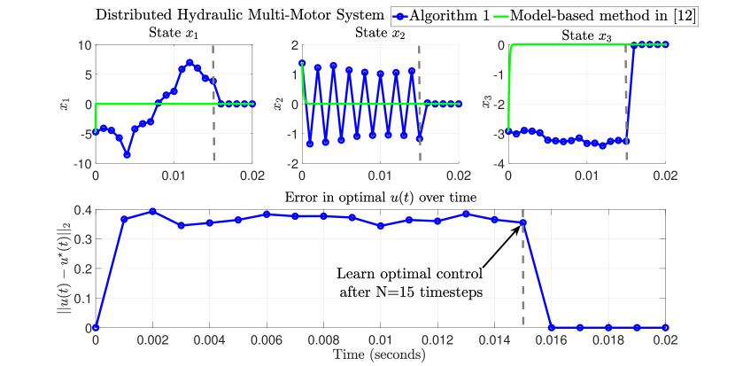
(b) Example V.2.

Figure 1: Performance of Algorithm 1 for (a) a Nuclear Fission Reactor system [5] and (b) a 2-motor Hydraulic system [24].

The optimal control sequence $u_{N}^{\infty}$, starting from an initial condition $x(N)$, obtained from the model-free PMP conditions is not guaranteed to be globally optimal just based on our derivations from (8). We utilize Theorem 1 to show global optimality of the input sequence ${u}_{N}^{t_{f}}$ as $t_{f}\to\infty$.

Lemma 3 (Convergence to a Limiting Solution $\hat{P}^{\star}(t,0)$)

For a known $x(t)$ at time $t$ and $T\gg 0$, $\lim_{T\to 0}P(t,{T})=\hat{P}^{\star}(t,0)$ that yields an optimal gain $\hat{K}_{t}^{\star}$ satisfying

$$\begin{split}&\hat{K}_{t}^{\star}={K}^{\star}(x(t))=-(\hat{P}^{\star}(t,0))_{mm}^{-1}(\hat{P}^{\star}(t,0))_{nm}^{T},\end{split}$$ (16)

where $\hat{K}^{\star}_{t}$ and $\hat{P}^{\star}(t,0)$ are the unique optimal solutions to (9a) and (15), respectively.

Proof:

Firstly, $\hat{K}^{\star}_{t}$ is the minimizer given that the sufficient second-order condition: ${\partial^{2}H^{\gamma}_{t}}/{\partial\hat{K}_{t}^{2}}=2G(x(t-1))S(t-1)G^{T}(x(t-1))(P(t,T))_{mm}\succeq 0$ holds since $(P(t,T))_{mm}\succ 0$ for all $T\geq 0$. For a fixed point $x(t)$ at time $t$ giving $\hat{U}(\hat{K}_{t})$ in (15), [25, Theorem 2.4-1, pg. 71] permits us to prove that $P(t,T)$ smoothly converges to a unique limiting solution $\hat{P}^{\star}(t,0)$ as $T\to 0$ given $P(t,T)=\Lambda\succeq 0$. Since $\lim_{T\to 0}P(t,T)=P^{\star}(t,0)$, then $\hat{K}_{t}(T)\to\hat{K}_{t}^{\star}$ which is the unique limiting solution to (16). ∎

Remark 2

We emphasize that we analyze the convergence and optimality properties at each point $x(t)$ for the bilinear system. With this in mind, we specifically leverage the established convergence proof for dynamic programming in [25, Theorem 2.4-1, pg. 71] to prove the result in Lemma 3.

Theorem 1

Algorithm 1 yields a globally optimal control policy $u(t)=K^{\star}(x(t))x(t)$ for all $t\geq N$ starting from an initial condition $x(N)$.

Proof:

At $t\geq N$, Algorithm 1 converges to the limiting solution ${K}^{\star}(x(t))$ which is unique for $x(t)$ such that $H_{t}^{\gamma}(K^{\star}(x(t)))\leq H_{t}^{\gamma}(K(x(t)))$. Then for all $t\in[N,\infty)$, $H_{t}^{\gamma}(K^{\star}(x(t)))\leq H_{t}^{\gamma}(K(x(t))$, which means that the state-input trajectory generated by the control law $u(t)=K^{\star}(x(t))x(t)$ is globally optimal starting from $x(N)$. ∎

V Numerical Examples

In this section, we demonstrate the efficacy of the proposed Model-Free Q-Learning Algorithm, Algorithm 1, and compare with the model-based algorithm in [12], in which the bilinear system is completely known.

Example V.1. Fission in Nuclear Reactors[5]: With a neutron population level $x_{1}(t)$ and neutron precursor (unstable fission products) $x_{2}(t)$, the discretized point neutron dynamics from nuclear fission is described as a bilinear model as in (1) with

$$\begin{split}&A=\begin{bmatrix}\frac{1-T_{s}}{l}&\lambda T_{s}\\ 0&1-\lambda T_{s}\end{bmatrix},D_{1}=\begin{bmatrix}\frac{1-\beta}{l}\\ \frac{\beta}{l}\end{bmatrix}T_{s},\end{split}$$ (17)

$B=D_{2}=\mathbf{0}$, and $T_{s}=0.001$s is the sampling time. The precursor portion, $\beta=0.157\times 10^{-3}$, has a neutron generation time $l=8.36\times 10^{-4}$s and a decay constant $\lambda=0.0120\text{s}^{-1}$. The input $u(t)\in\mathbb{R}$ is the adjustable neutron multiplicative factor used to control the rate of the nuclear chain reaction. We attempt to quickly stabilize the neutron population by choosing $\Lambda=diag(1,0,0.1)$ and $\gamma=0.9$. We use the results in in [15] to verify the span reachability of (17).

Example  V.2. Hydraulic Rotary Multi-motor System [24]: The discretized (with sampling time $T_{s}=0.001$) hydraulic rotary system for two motors can be written as in (1) with

$$\begin{split}&A=\mathrm{diag}(0.99997,-0.99997,0.99997),\\ &B=\mathrm{diag}(200,6,10),\,D_{2}=\begin{bmatrix}0&-0.00007&0\\ 0&0&0\\ 0&0&0\end{bmatrix},\\ &D_{1}=\begin{bmatrix}0&0&0\\ 0&0&0\\ 0&0.03&0.03\end{bmatrix},D_{3}=\begin{bmatrix}0&0&-0.00007\\ 0&0&0\\ 0&0&0\end{bmatrix}\end{split}$$ (18)

The state vector is comprised of the pressure level in the line-network, $x_{1}(t)$, and the speed of the first and second motor, $x_{2}(t)$ and $x_{3}(t)$ respectively. The inputs are the displacement volumes of the hydraulic pump, the first motor, and second motor respectively. We set $\Lambda=I_{6}$, and $\gamma=0.9$. Note that the square system (18) is span reachable according to [16].

Discussion of Results: Figures 1(a) and 1(b) show the comparative performance results of Algorithm 1 and the model-based algorithm in [12] for the Nuclear Fission Reactor system and the Multi-motor Hydraulic system, respectively. The model-based algorithm in [12] knows the complete bilinear dynamics a priori. As expected, the model-based algorithm in [12] outperforms our method since Algorithm 1 uses the first $N=5$ and $N=15$ respective time steps to collect data before learning the optimal policy. Thus, there is a suboptimal $Q$-cost accrued by Algorithm 1 as compared to that of the model-based method in [12]. The lower plots in each figure shows that Algorithm 1 computes a suboptimal control policy initially before learning the policy, globally optimal from this point $x(N)$, which stabilizes the respective system.

VI Conclusion

In this paper, we investigated the specific properties of Persistency of Excitation and Sufficient Richness under which the state-input data can characterize the span of range of possible system behaviors. By leveraging these specific properties, we developed a provably convergent online Model-Free $Q$-Learning algorithm that iteratively learns a stabilizing state-dependent optimal control policy for an unknown bilinear system from a single online run. Through two numerical examples, we demonstrated the efficacy of the proposed algorithm as compared to a model-based method in which the complete bilinear model is known. Future work will study the extension to the general (possibly noisy) control-affine nonlinear system which can be bilinearized.

References

- [1] N. Fulton and A. Platzer, “Safe Reinforcement Learning via Formal Methods: Toward Safe Control Through Proof and Learning,” in AAAI, 2018, pp. 6485–6492.
- [2] D. Lee and J. Hu, “Primal-Dual Q-Learning Framework for LQR design,” IEEE Transactions on Automatic Control, vol. 64, no. 9, pp. 3756–3763, 2018.
- [3] W. J. Rugh, Nonlinear system theory. Johns Hopkins University Press Baltimore, 1981.
- [4] C. Bruni, G. DiPillo, and G. Koch, “Bilinear Systems: An Appealing Class of “ Nearly Linear” Systems in Theory and Applications,” IEEE Transactions on Automatic Control, vol. 19, no. 4, pp. 334–348, 1974.
- [5] R. R. Mohler, “Natural Bilinear Control Processes,” IEEE Transactions on Systems Science and Cybernetics, vol. 6, no. 3, pp. 192–197, 1970.
- [6] D. Goswami and D. A. Paley, “Bilinearization, Reachability, and Optimal Control of Control-Affine Nonlinear Systems: A Koopman Spectral Approach,” IEEE Transactions on Automatic Control, 2021.
- [7] Z. Yuan and J. Cortés, “Data-Driven Optimal Control of Bilinear Systems,” IEEE Control Systems Letters, vol. 6, pp. 2479–2484, 2022.
- [8] A. Bisoffi, C. De Persis, and P. Tesi, “Data-based Stabilization of Unknown Bilinear Systems with Guaranteed Basin of Attraction,” Systems & Control Letters, vol. 145, p. 104788, 2020.
- [9] I. Markovsky, “Data-Driven Simulation of Generalized Bilinear Systems via Linear Time-invariant Embedding,” IEEE Transactions on Automatic Control, 2022.
- [10] D.-x. Gao and P.-p. Yang, “The Successive Approximation Procedure for Finite-time Optimal Control of Bilinear Systems with Disturbances,” in 2010 8th World Congress on Intelligent Control and Automation. IEEE, 2010, pp. 3560–3564.
- [11] G. Bitsoris and N. Athanasopoulos, “Constrained Stabilization of Bilinear Discrete-Time Systems Using Polyhedral Lyapunov Functions,” IFAC Proceedings Volumes, vol. 41, no. 2, pp. 2502–2507, 2008, 17th IFAC World Congress.
- [12] S. Wang and J.-S. Li, “Free-Endpoint Optimal Control of Inhomogeneous Bilinear Ensemble Systems,” Automatica, pp. 306–315, 2018.
- [13] R. Luesink and H. Nijmeijer, “On the Stabilization of Bilinear systems via Constant Feedback,” Linear algebra and its Applications, vol. 122, pp. 457–474, 1989.
- [14] Y. Zhao and J. Cortés, “Gramian-based Reachability Metrics for Bilinear Networks,” IEEE Transactions on Control of Network Systems, vol. 4, no. 3, pp. 620–631, 2016.
- [15] L. Tie, “Invariant sets and Controllability of Discrete-Time Bilinear Systems,” IET Control Theory & Applications, vol. 12, no. 7, pp. 970–979, 2018.
- [16] T. Nomura and K. Furuta, “On the Span Reachability of Polynomial State-Affine Systems,” IEEE Transactions on Automatic Control, vol. 24, no. 4, pp. 630–632, 1979.
- [17] G. Gu, Discrete-Time Linear Systems: Theory and Design with Applications. Springer US, 2012.
- [18] J. M. Conrad, C. W. Clark, et al., Natural Resource Economics: Notes and Problems. Cambridge University Press, 1987.
- [19] B. D. Anderson and J. B. Moore, Optimal Control: Linear Quadratic Methods. Courier Corporation, 2007.
- [20] E.-W. Bai and S. S. Sastry, “Persistency of excitation, sufficient richness and parameter convergence in discrete time adaptive control,” Systems & control letters, vol. 6, no. 3, pp. 153–163, 1985.
- [21] I. M. Jan C. Willems, Paolo Rapisarda and B. De Moor, “A Note on Persistency of Excitation,” Systems and Control Letters, vol. 54, no. 4, pp. 325–329, 2005.
- [22] K. Conrad, “Tensor products,” Notes of course, available on-line, 2018. [Online]. Available: https://kconrad.math.uconn.edu/blurbs/linmultialg/tensorprod.pdf
- [23] Y. Zhu, Multivariable System Identification for Process Control. Elsevier, 2001.
- [24] H. R. Shaker and J. Stoustrup, “An Interaction Measure for Control Configuration Selection for Multivariable Bilinear Systems,” Nonlinear Dynamics, vol. 72, no. 1, pp. 165–174, 2013.
- [25] F. L. Lewis, D. Vrabie, and V. L. Syrmos, Optimal control. John Wiley & Sons, 2012.