Benchmarking magnetized three-wave coupling for laser backscattering: Analytic solutions and kinetic simulations

Abstract

Understanding magnetized laser-plasma interactions is important for controlling magneto-inertial fusion experiments and developing magnetically assisted radiation and particle sources. In the long-pulse regime, interactions are dominated by coherent three-wave interactions, whose nonlinear coupling coefficients become known only recently when waves propagate at oblique angles with the magnetic field. In this paper, backscattering coupling coefficients predicted by warm-fluid theory is benchmarked using particle-in-cell simulations in one spatial dimension, and excellent agreements are found for a wide range of plasma temperatures, magnetic field strengths, and laser propagation angles, when the interactions are mediated by electron-dominant hybrid waves. Systematic comparisons between theory and simulations are made possible by a rigorous protocol: On the theory side, the initial boundary value problem of linearized three-wave equations is solved, and the transient-time solutions allow effects of growth and damping to be distinguished. On the simulation side, parameters are carefully chosen and calibration runs are performed to ensure that stimulated runs are well controlled. Fitting simulation data to analytical solutions yields numerical growth rates, which match theory predictions within error bars. Although warm-fluid theory is found to be valid for a wide parameter range, genuine kinetic effects have also been observed.

1 Introduction

Laser-plasma interactions (LPI) are usually studied without a background magnetic field, partly because the relevant field strengths are over hundreds of teslas that are difficult to attain, and partly because cyclotron motion significantly complicates physical processes making the interactions difficult to understand. However, in recent experiments where a seed magnetic field is imposed to enhance thermal and particle confinements in laser-driven inertial fusion experiments (chang2011fusion; hohenberger2012inertial), understanding magnetized LPI (MagLPI) have become necessary. In experiments that are designed using codes that incorporate magnetization effects on hydrodynamics but not including magnetization effects on LPI, the observed hot spot shape is more elongated along the magnetic field than expected (Moody22). Subsequent experiments using manually adjusted laser drive manage to restore the symmetry, suggesting that MagLPI is one of the likely causes of the discrepancy.

Strong magnetic fields directly affect LPI in addition to changing plasma conditions. In indirect-drive experiments, external coils apply a seed magnetic field of $B_{0}\approx 30$ T, which is not particularly strong. However, during the laser drive, expanding plasmas from the hohlraum wall compresses the magnetic flux near the laser entrance hole, causing the magnetic field there to be amplified to $100$-T level (strozzi2015imposed). Moreover, Biermann-battery fields near the laser spot and flux compression due to the imploding fuel lead to even larger fields at kT-level (knauer2010compressing; sio2021diagnosing). When $B_{0}\sim 10^{2}$ T, electron cyclotron frequency becomes comparable to the frequency of sound waves that mediate Brillouin scattering and crossbeam laser energy transfer. Moreover, when $B_{0}\sim 10^{3}$ T, electron cyclotron frequency becomes comparable to plasma frequency, leading to modifications of the Langmuir wave that mediates Raman scattering and two-plasmon decay. The ability to explain and predict magnetized version of these commonly encountered long-pulse LPI processes rely on basic understandings of MagLPI that we have just begun to acquire.

While basic facts about unmagnetized LPI, such as the linear growth rates of Raman and Brillouin scatterings, are well known from decades of theoretical, numerical, and experimental studies, simple facts about MagLPI are poorly understood. The two exceptions are when waves propagate either perpendicular or parallel to the background magnetic field. Perpendicular propagation is particularly relevant for magnetic confinement fusion, where strong radio-frequency pump waves are used for plasma heating and current drive. Using antenna mounted on vacuum chamber walls, the waves are launched nearly perpendicular to the magnetic field. In this geometry, the extraordinary (X) pump can decay to upper-hybrid (UH) and lower-hybrid (LH) waves (grebogi1980brillouin; hansen2017parametric), as well as couple with Bernstein waves (Platzman68; Stenflo81). The other special geometry is when waves propagate nearly parallel to the magnetic field, which is particularly relevant for astrophysical type plasmas, where the pump wave is an Alfvén wave whose frequency is below cyclotron frequencies. In this case, the pump can couple with sound waves and other Alfvén type waves (hasegawa1976kinetic; wong1986parametric), and the coupling is known also at oblique angles (vinas1991parametric). In the context of LPI, the pump waves are lasers, whose frequencies are typically higher than electron-cyclotron frequency. Most studies of MagLPI also focus on special geometry where theories are greatly simplified. In the perpendicular geometry, X-wave pump lasers undergo backscattering (paknezhad2016effect; shi2017laser), forward scattering (hassoon2009stimulated; babu2021stimulated), second harmonics generation (jha2007second), and THz radiation generation (varshney2015strong). In the parallel geometry, the electrostatic waves are unmagnetized but the right-handed (R) and left-handed (L) circularly polarized electromagnetic waves become nondegenerate, changing the coupling for Raman and Brillouin type scatterings (sjolund1967non; laham1998effects). In more general geometry, where waves propagate at oblique angles with respect to the magnetic field, cyclotron motion makes theoretical analysis significantly more complicated. Although theories exist (larsson1973three; liu1986parametric; stenflo1994resonant; brodin2012three), the coupling coefficients are given by cumbersome formulas that are general but rarely evaluated. Physical understanding of underlying processes are largely lacking until recently when more convenient formulas are obtained and evaluated (Shi17; Shi19), leading to pictures of MagLPI that are both intuitive and quantitative (shi2018laser; shi2021plasma). However, it remains unclear how accurate are these formulas and to what extent are they applicable. Because lasers propagate at oblique angles in inertial fusion experiments, it is especially important to known whether the predicted couplings are correct beyond special angles.

To benchmark analytical formulas, kinetic simulations have been used but systematic comparisons are difficult. When waves propagate perpendicular (boyd1985kinetic; jia2017kinetic) or parallel (li2020boosting; li2021boosting) to the magnetic field, qualitative agreements between theories and simulations have been found. Moreover, at oblique angles, it is observed that even in regimes where kinetic effects are expected to be important, coupling coefficients predicted by warm-fluid theory are indictive of kinetic simulation results (edwards2019laser; Manzo22). However, systematic comparisons between theory and simulations of MagLPI have not been made, which is the goal of this paper. Making the comparisons rigorous is difficult due to three reasons. First, nonlinear coupling leads to wave growth, but the effect of growth is mixed with damping in kinetic simulations. In the absence of collision, magnetized plasma waves are still damped collisionlessly, whose rate is difficult to calculate because cyclotron motion mixes with trapping motion and particle trajectories are chaotic in general. Even in the simple perpendicular geometry, the two limiting cases, where trapping motion dominates cyclotron motion (sagdeev1973influence; dawson1983damping) or vice versa (karney1978stochastic; karney1979stochastic), have drastically different behavior, and the intermediate regimes are far less understood. Since a larger damping can offset a larger growth, their effects need to be separated before coupling coefficients can be constrained. Second, the coupling coefficients derived in theories are specific for eigenmodes but launching eigenmodes in kinetic simulations is not straightforward when waves propagate at oblique angles. In previously simulations, the pump laser is launched with simple linear or circular polarizations from the vacuum region. Upon entering the magnetized plasma, which is a birefringent medium, the laser excites both eigenmodes, which are elliptically polarized at oblique angles. Since nonlinear couplings are different depending on the laser polarization (shi2019amplification), exciting multiple modes does not allow a clean comparison. Finally, additional processes can occur in kinetic simulations, making it difficult to isolate the process of interest. For example, the pump laser can undergo spontaneous scattering into other modes. This problem is particularly severe in particle-in-cell (PIC) simulations, where Monte Carlo sampling noise cause unphysically large spontaneous scattering. As another problem, collisionless damping causes the distribution function to evolve on a time scale that is often comparable to wave growth, which is an issue for both PIC and Vlasov simulations. Since coupling coefficients depend on the distribution function, its time evolution complicates the comparison between theories and simulations.

In this paper, one dimensional PIC simulations are used to benchmark coupling coefficients predicted by warm-fluid theory, and excellent agreements between simulations and theory are achieved using a protocol that enables quantitative comparisons. First, to distinguish effects of damping from growth, analytical solutions of the linearized three-wave equation are derived in Sec. 2 and are used to fit simulations data. Building up solutions from initial value problem to boundary value problem, the transient-time spatial profiles in the backscattering problem, where a seed laser is amplified by a counter propagating pump laser, allows damping and growth rates to be constrained separately. Second, to make numerical results directly comparable to theory, calibration steps are performed for PIC simulations, which are described in Sec. 3. To ensure that a single eigenmode is excited, the pump and seed laser polarizations are calibrated. To account for laser reflections from plasma-vacuum boundaries, laser transmissions are calibrated. To separate pump and seed from raw data and extract their envelopes, phase velocities are calibrated. These calibration runs eliminate free parameters during fitting and make the stimulated run well controlled. Third, competing processes are monitored to ensure that only valid data are used for fitting. Simulation parameters are chosen to reduce the impacts of spontaneous scattering, and the seed wavelength is scanned to excite leading resonances, which are mediated by the Langmuir-like P wave and the electron-cyclotron-like F wave. In addition, evolution of distribution function is monitored to select data within a time window where plasma conditions remain constant. Fitting well-controlled simulation data to analytical solutions of the same setup leads to excellent agreements in Sec. LABEL:Sec:Results, where the warm-fluid theory is shown to be valid within a wide parameter range. The protocol has difficulties for weak resonances, primarily due to spontaneous scattering and leakages during pump-seed separation. Potential ways to circumvent the difficulties are discussed in Sec. LABEL:Sec:Discussion, and further investigations may find that the warm-fluid theory is valid in even wider parameter spaces. Nevertheless, kinetic effects such collisionless damping and Bernstein-like resonances are clearly observed, suggesting the importance of developing and benchmarking kinetic theories of MagLPI in the future.

2 Analytic solutions of linearized three-wave equations

In the slowly-varying amplitude approximation $E=\mathcal{E}\sin\theta$, where the wave envelop $\mathcal{E}$ varies slowly compared to the wave phase $\theta=\mathbf{k}\cdot\mathbf{x}-\omega t+\theta_{0}$, the interaction between three resonant waves, which satisfy $\omega_{1}=\omega_{2}+\omega_{3}$ and $\mathbf{k}_{1}=\mathbf{k}_{2}+\mathbf{k}_{3}$, is described by the three-wave equations d_t a_1 & = -Γω1 a_2 a_3,
d_t a_2 = Γω2 a_1 a_3,
d_t a_3 = Γω3 a_1 a_2, where $d_{t}=\partial_{t}+\mathbf{v}\cdot\nabla+\mu$ is the advective derivative at group velocity $\mathbf{v}=\partial\omega/\partial\mathbf{k}$ and $\mu$ is a phenomenological damping rate. The above equations describe the decay of pump wave $a_{1}$ into daughter waves $a_{2}$ and $a_{3}$, and the inverse process. The dimensionless $a=e|\mathbfcal{E}|u^{1/2}/m_{e}\omega c$ is the normalized electric-field amplitude. The normalization is such that when $a>1$, the quiver velocity of electrons, whose charge is $-e$ and mass is $m_{e}$, becomes comparable to the speed of light $c$. The normalization also involves the wave-energy coefficient $u=\frac{1}{2}\mathbf{e}^{\dagger}\mathbb{H}\mathbf{e}$, where $\mathbb{H}$ is the Hamiltonian of linear waves and $\mathbf{e}$ is the unit polarization vector, such that the cycle-averaged energy of the wave is $\frac{1}{2}\epsilon_{0}u\mathbfcal{E}^{2}$. The wave-energy coefficient is simply $u=1$ for unmagnetized electromagnetic waves and cold Langmuir waves. However, for magnetized plasma waves, $u$ usually differs from unity and can be evaluated using the code in Shi22 for given eigenmodes.

The key parameter in the three-wave equation is the coupling coefficient $\Gamma$, which has units of frequency squared. In magnetized warm-fluid plasmas, $\Gamma$ is given by the explicit formula (Shi17; Shi19)

$$\Gamma=\sum_{s}\frac{Z_{s}\omega_{ps}^{2}(\Theta^{s}+\Phi^{s})}{4M_{s}(u_{1}u_{2}u_{3})^{1/2}},$$ (1)

where the summation is over all plasma species, with normalized charge $Z_{s}=e_{s}/e$, mass $M_{s}=m_{s}/m_{e}$, and plasma frequency $\omega_{ps}^{2}=e_{s}^{2}n_{s0}/\epsilon_{0}m_{s}$ at equilibrium density $n_{s0}$. In the numerator, $\Theta$ is due to electromagnetic scattering and is equals to the sum of $\Theta_{1,\bar{2}\bar{3}}$ with its five permutations. Explicitly, $\Theta_{i,jl}=\frac{1}{\omega_{j}}(c\mathbf{k}_{i}\cdot\mathbf{f}_{j})(\mathbf{e}_{i}\cdot\mathbf{f}_{l})$, where $\mathbf{f}=\mathbb{F}\mathbf{e}$ and $\mathbb{F}$ is related to the linear susceptibility by $\chi=-\omega_{p}^{2}\mathbb{F}/\omega^{2}$, which reduces to $\mathbb{F}=\mathbb{I}$ for unmagnetized cold plasmas. The notation $\bar{i}$ in subscripts means complex conjugation for $\mathbf{e}_{i}$ and $\mathbf{f}_{i}$ with negations for the wave 4-momentum $(\omega_{i},\mathbf{k}_{i})$. Finally, the $\Phi$ term in Eq. (1) is due to warm-fluid nonlinearities, which is typically smaller than $\Theta$ by a factor of $v_{T}^{2}/c^{2}$, where $v_{T}$ is thermal speed. The coupling coefficient can be readily evaluated using the code in Shi22 once plasma conditions and the three resonant waves are specified.

To benchmark the value of magnetized three-wave coupling coefficient $\Gamma$ using numerical simulations, this paper considers a linearized and one-dimensional problem whereby the three-wave equations are simplified. First, the pump wave is launched with an amplitude that is much larger than the daughter waves, in which case $a_{1}$ remains approximately a constant. Second, simulations in one spatial dimension are used, meaning that $\mathbf{k}\parallel\hat{\mathbf{x}}$ and the wave envelopes only vary along the $x$ direction. Notice that the group velocity $\mathbf{v}$ can have components in other directions, but $\mathbf{v}\cdot\nabla$ only picks up its $x$ component $v$. With these simplifications, Eqs. (2) becomes a coupled-mode equation $\mathsfbi{L}\ubalpha=\mathbf{0}$ where

$$\mathsfbi{L}=\left(\begin{array}[]{cc}\partial_{t}+v_{2}\partial_{x}+\mu_{2}&-\gamma_{0}\\ -\gamma_{0}&\partial_{t}+v_{3}\partial_{x}+\mu_{3}\end{array}\right),$$ (2)

and $\ubalpha=(\alpha_{2},\alpha_{3})^{\mathrm{T}}$ is a column vector. Here, $\alpha=\sqrt{\omega}a$ is rescaled such that the off diagonal elements are the same $\gamma_{0}$. Since only $\gamma_{0}^{2}$ is of physical significance, we can pick the positive sign so that the bare growth rate of daughter waves is

$$\gamma_{0}=\frac{|\Gamma a_{1}|}{\sqrt{\omega_{2}\omega_{3}}}.$$ (3)

Without loss of generality, we can always choose to label the daughter waves such that $|v_{2}|\geq|v_{3}|$. Moreover, we can always choose a coordinate such that $v_{2}\geq 0$. With these choices, $\Delta v=v_{2}-v_{3}\geq 0$ is nonnegative. Solutions to $\mathsfbi{L}\ubalpha=\mathbf{0}$ are different in forward ($v_{3}>0$) and backward ($v_{3}<0$) scattering cases.

Since the equations are linear, they admit exponential solutions that are simple to write down analytically but difficult to set up numerically. The exponential solutions are of the form $\alpha_{2}\propto\alpha_{3}\propto\exp(\gamma t+\kappa x)$ where the temporal and spatial growth rates satisfy

$$(\gamma+v_{2}\kappa+\mu_{2})(\gamma+v_{3}\kappa+\mu_{3})=\gamma_{0}^{2}.$$ (4)

The above constraint defines a hyperbola in the $(\kappa,\gamma)$ plane. One special case is $\kappa=0$, where the wave envelopes are uniform in space. The two roots are $\gamma_{\pm}=-\bar{\mu}\pm\Omega$, where $\bar{\mu}=\frac{1}{2}(\mu_{2}+\mu_{3})$, $\Omega=\sqrt{\gamma_{0}^{2}+(\frac{\Delta\mu}{2})^{2}}$, and $\Delta\mu=\mu_{2}-\mu_{3}$. When $\gamma_{0}<\gamma_{c}$, both roots are negative and correspond to damping. On the other hand, when $\gamma_{0}>\gamma_{c}$, one root becomes positive, giving rise to parametric instability whose threshold is

$$\gamma_{c}=\sqrt{\mu_{2}\mu_{3}}.$$ (5)

The other special case is $\gamma=0$, where the wave envelopes are stationary in time. Assuming $v_{2}v_{3}\neq 0$, then for forward scattering $v_{2}v_{3}>0$, the envelopes decay in space unless $\gamma_{0}>\gamma_{c}$, similar to the previous case. However, the backscattering case $v_{2}v_{3}<0$ is very different: Purely growing or decaying solution no longer exists when $\gamma_{0}$ exceeds the absolute instability threshold

$$\gamma_{a}=\frac{1}{2}\sqrt{|v_{2}v_{3}|}\Big{(}\frac{\mu_{2}}{|v_{2}|}+\frac{\mu_{3}}{|v_{3}|}\Big{)}.$$ (6)

When $\gamma_{0}>\gamma_{a}$, the two roots of $\kappa$ acquire imaginary parts, which means that stationary exponential solutions become oscillatory in space. The significance of $\gamma_{a}$ will become apparent in Eq. (2.3) when we discuss the backscattering problem. To extract growth rates from kinetic simulations, which are usually designed to solve initial boundary value problems, one approach is to choose an initial condition that corresponds to a uniform $\alpha$ and watch it grow in time. However, the effect of growth is mixed with damping, whose rate is unknown when waves propagate at oblique angles with the magnetic field. An alternative approach is to run simulations until the system reaches steady state. However, the plasma distribution functions also evolve during the process, sometimes quite substantially (Manzo22), so the growth and damping are not only mixed but are also not constants. To overcome these difficulties, kinetic simulations are fitted using more general solutions of $\mathsfbi{L}\ubalpha=\mathbf{0}$ by solving initial boundary value problems, whose solutions are known (bobroff1967impulse; mounaix1994space; hinkel1994temporal) but are rederived below for clarity. The spatial variations of $\alpha$ allow the effects of growth and damping to be distinguished, and the transient-time response before plasma conditions evolve allows the growth and damping rates to be treated as constants.

2.1 Initial value problem

In the initial value problem, the spatial domain is infinite, and the wave envelops evolve in time from their initial conditions

$$\ubalpha(x,t=0)=\mathbf{A}(x),$$ (7)

where $\mathbf{A}=(A_{2},A_{3})^{\mathrm{T}}$. In the degenerate case $v_{2}=v_{3}=v$, after transforming to the comoving frame $x^{\prime}=x-vt$ and $t^{\prime}=t$ where $\partial_{t}+v\partial_{x}=\partial_{t^{\prime}}$, the equations become ordinary differential equations (ODEs) in $t^{\prime}$. The eigenvalues $\gamma_{\pm}=-\bar{\mu}\pm\Omega$ of the linear ODEs are the $\kappa=0$ roots of Eq. (4), and the general solutions are of the form $\alpha(x^{\prime},t^{\prime})=A_{+}(x^{\prime})e^{\gamma_{+}t^{\prime}}+A_{-}(x^{\prime})e^{\gamma_{-}t^{\prime}}$. The coefficients $A_{\pm}$ are determined by matching initial conditions, which give the solution

$$\ubalpha=e^{-\bar{\mu}t}\left(\begin{array}[]{cc}\cosh\Omega t-\frac{\Delta\mu}{2\Omega}\sinh\Omega t&\frac{\gamma_{0}}{\Omega}\sinh\Omega t\\ \frac{\gamma_{0}}{\Omega}\sinh\Omega t&\cosh\Omega t+\frac{\Delta\mu}{2\Omega}\sinh\Omega t\end{array}\right)\mathbf{A}(x-vt).$$ (8)

The above $\Delta v=0$ solution exhibits two features that are more general: a diagonal damping term, and off-diagonal coupling terms that vanish when $\gamma_{0}=0$. The rest of this paper will focus on the nondegenerate case $\Delta v>0$, because in LPI $v_{2}$ is close to the speed of light whereas $v_{3}$ is on the scale of thermal velocities, which are much slower.

In the nondegenerate case $\Delta v>0$, since the equations are linear, they can be solved using Fourier transform $\mathcal{F}[p](k)=\int_{-\infty}^{+\infty}dx\;p(x)\exp(-ikx)=\hat{p}(k)$. In momentum space, the equation becomes $\partial_{t}\hat{\ubalpha}=\mathsfbi{K}\hat{\ubalpha}$ where

$$\mathsfbi{K}=\left(\begin{array}[]{cc}-ikv_{2}-\mu_{2}&\gamma_{0}\\ \gamma_{0}&-ikv_{3}-\mu_{3}\end{array}\right).$$ (9)

Since the matrix is time independent, the solution is $\hat{\ubalpha}(t)=\exp(t\mathsfbi{K})\hat{\mathbf{A}}$. The matrix exponential can be computed by diagonalizing $\mathsfbi{K}$ whose eigenvalues are $\lambda_{\pm}=-ik\bar{v}-\bar{\mu}\pm\sqrt{\gamma_{0}^{2}-\omega^{2}}$, where $\bar{v}=\frac{1}{2}(v_{2}+v_{3})$ and $\omega=\frac{1}{2}(k\Delta v-i\Delta\mu)$. Finding eigenvectors of $\lambda_{\pm}$ and diagonalizing $\mathsfbi{K}$, the solution map $\hat{\Phi}(k,t)=\exp(t\mathsfbi{K})$ can be written as

$$\hat{\Phi}(k,t)=e^{-(ik\bar{v}+\bar{\mu})t}\left(\begin{array}[]{cc}\partial_{t}-i\omega&\gamma_{0}\\ \gamma_{0}&\partial_{t}+i\omega\end{array}\right)\hat{G}(k,t),$$ (10)

where $\hat{G}(k,t)=\sinh(t\sqrt{\gamma_{0}^{2}-\omega^{2}})/\sqrt{\gamma_{0}^{2}-\omega^{2}}$. The solution map $\hat{\Phi}(k,t)$ satisfies matrix equation $\partial_{t}\hat{\Phi}(k,t)=\mathsfbi{K}\hat{\Phi}(k,t)$ and initial condition $\hat{\Phi}(k,t=0)=\mathsfbi{I}$, where $\mathsfbi{I}$ is the two-dimensional identity matrix. Notice that the behavior of $\hat{G}$ is regular when $\omega(k)\rightarrow\pm\gamma_{0}$. We can choose the branch cut for the square roots to lie between these two points. Since $\sinh$ is an odd function, $\hat{G}$ is in fact analytic in the complex $k$ plane.

To find the solution in $x$ space, take inverse Fourier transform $\mathcal{F}^{-1}[\hat{p}](x)=\int_{-\infty}^{+\infty}\frac{dk}{2\pi}\hat{p}(k)e^{ikx}=p(x)$. Since $\omega$ depends on $k$, it is convenient to change the integration variable to $k^{\prime}=2\omega/\Delta v$, which gives $k=k^{\prime}+i\Delta\mu/\Delta v$. Moreover, it is convenient to change the reference frame to τ& = Δv2 t,
z = x-¯vt, which travels at the average velocity of the two waves. Notice that $z-\tau=x-v_{2}t$ and $z+\tau=x-v_{3}t$. The phase factor simplified as $\exp[ikx-(ik\bar{v}+\bar{\mu})t]=\rho e^{ik^{\prime}z}$ where

$$\rho=\exp\Big{\{}\frac{1}{\Delta v}\Big{[}\mu_{3}(z-\tau)-\mu_{2}(z+\tau)\Big{]}\Big{\}},$$ (11)

which is a damping factor independent of $k^{\prime}$. When taking inverse Fourier transform of Eq. (10), all matrix elements can be expressed in terms of g(z, τ) &= ∫_-∞-iϵ^+∞-iϵ dk’2π e^ik’zsinhτm2-k’2m2-k’2
= 12sign(τ)I_0(mτ^2-z^2)Θ(τ^2-z^2), where $m=2\gamma_{0}/\Delta v$, $I_{0}$ is modified Bessel function, and $\Theta$ is Heaviside step function. The shift by $\epsilon=\Delta\mu/\Delta v$ is insignificant because the integrand is analytic. The above integral is calculated in appendix LABEL:appA. The solution map $\Phi$ in configuration space is

$$\Phi(x,t)=\rho\left(\begin{array}[]{cc}\partial_{\tau}-\partial_{z}&m\\ m&\partial_{\tau}+\partial_{z}\end{array}\right)g(z,\tau).$$ (12)

The derivatives are evaluated using $I^{\prime}_{0}(\xi)=I_{1}(\xi)$ and $\Theta^{\prime}(\xi)=\delta(\xi)$, and an explicit formula is given by Eq. (LABEL:eq:PhixExplicit). The function $g$ satisfies the imaginary-mass Klein-Gordon equation $(\partial_{\tau}^{2}-\partial_{z}^{2}-m^{2})g(z,\tau)=0$, as shown in Eq. (LABEL:eq:gGreen). Consequently, the solution map satisfies $\mathsfbi{L}\Phi(x,t)=\mathsfbi{0}$ following Eq. (LABEL:eq:Drho). The step function $\Theta$ enforces the causality that information outside the light cone $\tau^{2}-z^{2}=(v_{2}t-x)(x-v_{3}t)$ does not affect solutions.

Finally, to invert $\hat{\ubalpha}=\hat{\Phi}\hat{\mathbf{A}}$, compute inverse Fourier transform of products, which are given by convolutions $\mathcal{F}^{-1}[\hat{p}\hat{q}](x)=\int_{-\infty}^{+\infty}dx^{\prime}\;p(x^{\prime})q(x-x^{\prime})$. Since the phase factor is simpler in $k^{\prime}=k-i\Delta\mu/\Delta v$, in addition to the change of variables in Eq. (2.1), it is convenient to define $\hat{\mathbf{B}}(k^{\prime})=\hat{\mathbf{A}}(k)$, which means that $\mathbf{B}(x)=\exp(x\Delta\mu/\Delta v)\mathbf{A}(x)$. With $\ubalpha=\rho\ubbeta$, where $\rho$ is given by Eq. (11), the solution can be written as β_2(z,τ) & = B_2(z​-​τ)+m2​∫_-τ^τ​dz’ [B_2(z​-​z’)τ​+​z’τ​-​z’I_1(ξ’)+B_3(z​+​z’)I_0(ξ’)],  
β_3(z,τ) = B_3(z​+​τ)+m2​∫_-τ^τ​dz’ [B_3(z​+​z’)τ​+​z’τ​-​z’I_1(ξ’)+B_2(z​-​z’)I_0(ξ’)],   where $\xi^{\prime}=m\sqrt{\tau^{2}-z^{\prime 2}}$. An explicit expression of $\ubalpha$ in $(x,t)$ coordinate is given later in Eq. (14). It is straightforward to check that the above expression satisfies the differential equation and the initial conditions. When $\mathbf{B}$ only involves $\delta$ or step functions, the above integrals can be readily evaluated. However, for general initial conditions, closed-form analytical expressions may not exist, so the above integrals is evaluated numerically. Compared to numerical integration of the differential equations, which advances initial conditions step by step, the above integral solution allows fast forwarding, which directly gives the solution at desired final time. Notice that by rescaling $z^{\prime}=\tau\zeta$, the numerical integration is always within the range $\zeta\in[-1,1]$, so the cost of evaluating the integral does not increase with time for smooth initial conditions.

2.2 Initial boundary value problem

Compared to the initial value problem, the boundary value problem is easier to set up in kinetic simulations. In the initial value problem, the distribution functions need to be specified meticulously in both the configuration space and the velocity space in order to ensure that only the desired eigenmodes are excited. In comparison, in boundary value problem, only electromagnetic fields at the boundary need to be specified. Using wave frequencies and polarizations to select excited waves, the desired eigenmodes then propagate into the initially Maxwellian plasma where interactions occur. With a single boundary at $x=0$, the initial boundary value problem is specified by the conditions (x¿0,t=0) & = A(x),
(x=0,t¿0) = h(t), where $\mathbf{h}=(h_{2},h_{3})^{\mathrm{T}}$. In the forward scattering case $v_{2}>v_{3}>0$, these conditions can be specified separately. However, in the backscattering case $v_{2}>0>v_{3}$, in order for the problem to be well-posed, only two conditions can be specified independently.

Since the equation $\mathsfbi{L}\ubalpha=\mathbf{0}$ is linear, the initial boundary value problem can be solved using Laplace transform $\mathcal{L}[p](k)=\int_{0}^{+\infty}dx\;p(x)\exp(-ikx)=\tilde{p}(k)$. Using property of the Laplace transform that $\tilde{p^{\prime}}(k)=ik\tilde{p}(k)-p(0)$, the equation becomes $\partial_{t}\tilde{\ubalpha}=\mathsfbi{K}\tilde{\ubalpha}+\mathbf{H}$, where $\mathsfbi{K}$ is given by Eq. (9) and $\mathbf{H}=(v_{2}h_{2},v_{3}h_{3})^{\mathrm{T}}$ only depends on time. Using the Duhamel’s principle, the inhomogeneous ODE is solved by $\tilde{\ubalpha}(t)=\hat{\Phi}(t)\tilde{\mathbf{A}}+\int_{0}^{t}dt^{\prime}\hat{\Phi}(t-t^{\prime})\mathbf{H}(t^{\prime})$, where $\hat{\Phi}$ is given by Eq. (10). To find the solution in configuration space, take inverse Laplace transform $\mathcal{L}^{-1}[\hat{p}\tilde{q}](x)=\int_{\mathcal{C}}\frac{dk}{2\pi}\mathcal{F}[p](k)\mathcal{L}[q](k)e^{ikx}=\int_{0}^{+\infty}dx^{\prime}p(x-x^{\prime})q(x^{\prime})$, where the contour $\mathcal{C}$ runs below all poles. The solution is

$$\ubalpha(x,t)=\int_{0}^{\infty}dx^{\prime}\Phi(x-x^{\prime},t)\mathbf{A}(x^{\prime})+\int_{0}^{t}dt^{\prime}\Phi(x,t-t^{\prime})\mathbf{H}(t^{\prime}),$$ (13)

where $\Phi$ is given by Eq. (12). Using $\mathsfbi{L}\Phi=\mathsfbi{0}$, the above expression clearly satisfies $\mathsfbi{L}\ubalpha=\mathbf{0}$. Moreover, using the explicit expression of $\Phi$ in Eq. (LABEL:eq:PhixExplicit), it is easy to see that $\Phi(x,t=0)=\delta(x)\mathsfbi{I}$, so the initial conditions are always satisfied. However, the situation for boundary conditions depends on the sign of $v_{3}$, as we shall see below.

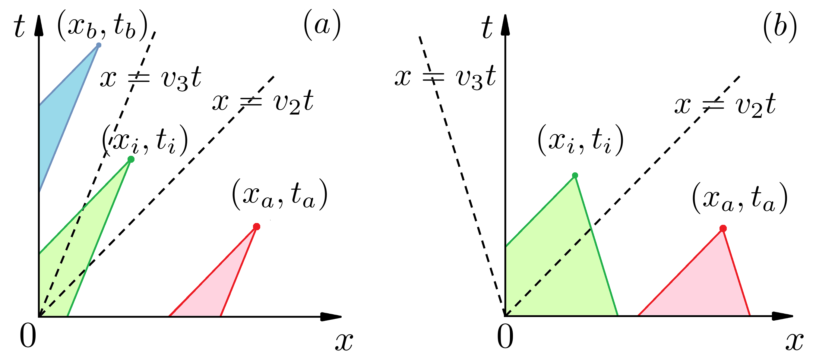
Figure 1: Solutions are determined by initial and boundary conditions within the past light cone. For $(x_{a},t_{a})$ ahead of $x>v_{2}t$, the light cone (red) only intercepts the $x$ axis, so the solution is independent of boundary conditions. For $(x_{b},t_{b})$ behind $x<v_{3}t$, the light cone (blue) only intercepts the $t$ axis, so the solution is independent of initial conditions. For $(x_{i},t_{i})$ within $v_{3}t<x<v_{2}t$, the solution depends on both initial and boundary conditions. $(a)$ In the forward scattering case, initial and boundary conditions can be specified independently. $(b)$ In the backscattering case, initial conditions arrive at the boundary so constraints must be satisfied.

Using the property that $\Phi$ is zero outside the light cone, the above integral solution, which is equivalent to $\ubalpha(x,t)=\int_{-\infty}^{x}dx^{\prime}\Phi(x^{\prime},t)\mathbf{A}(x-x^{\prime})+\int_{0}^{t}dt^{\prime}\Phi(x,t^{\prime})\mathbf{H}(t-t^{\prime})$, is simplified in the three regions shown in figure 1. First, ahead of the light cone $x>v_{2}t$, effects of boundary conditions have not arrived, so only the initial conditions contribute. In terms of the rescaled variable $\ubbeta$, the solution is given by Eq. (2.1), and in terms of the original variables, the solution when $x>v_{2}t>0$ is

$$\ubalpha(x,t)=\left(\begin{array}[]{c}e^{-\mu_{2}t}A_{2}(x-v_{2}t)\\ e^{-\mu_{3}t}A_{3}(x-v_{3}t)\end{array}\right)+\frac{\gamma_{0}}{\Delta v}\int_{v_{3}t}^{v_{2}t}dx^{\prime}\rho(x^{\prime},t)\Phi_{0}(x^{\prime},t)\mathbf{A}(x-x^{\prime}),$$ (14)

where $\rho$ is the damping factor given by Eq. (11) and $\Phi_{0}$ is the kernel within the light cone given in Eq. (LABEL:eq:PhixExplicit). When $t=0$, the solution clearly satisfies the initial conditions. Second, behind the light cone $x<v_{3}t$, which is within the domain only when $v_{3}>0$, effects of the initial conditions have propagated away, so only the boundary conditions contribute. Therefore, when $v_{3}t>x>0$, the solution is

$$\ubalpha(x,t)=\left(\begin{array}[]{c}e^{-\mu_{2}x/v_{2}}h_{2}(t-x/v_{2})\\ e^{-\mu_{3}x/v_{3}}h_{3}(t-x/v_{3})\end{array}\right)+\frac{\gamma_{0}}{\Delta v}\int_{x/v_{2}}^{x/v_{3}}dt^{\prime}\rho(x,t^{\prime})\Phi_{0}(x,t^{\prime})\mathbf{H}(t-t^{\prime}).$$ (15)

The solution clearly satisfies the boundary conditions at $x=0$ for this forward scattering case. Finally, inside the light cone, both the initial and boundary conditions contribute, and the solution when $v_{3}t<x<v_{2}t$ is given by

$$\ubalpha(x,t) = \left(\begin{array}[]{c}e^{-\mu_{2}x/v_{2}}h_{2}(t-x/v_{2})\\ e^{-\mu_{3}t}A_{3}(x-v_{3}t)\end{array}\right)$$ (18)

$$+ \frac{\gamma_{0}}{\Delta v}\int_{v_{3}t}^{x}dx^{\prime}\rho(x^{\prime},t)\Phi_{0}(x^{\prime},t)\mathbf{A}(x-x^{\prime})$$

$$+ \frac{\gamma_{0}}{\Delta v}\int_{x/v_{2}}^{t}dt^{\prime}\rho(x,t^{\prime})\Phi_{0}(x,t^{\prime})\mathbf{H}(t-t^{\prime}).$$

In the forward scattering case $v_{3}>0$, the future light cone is within the domain, so the initial and boundary conditions can be specified independently. However, in the backscattering case $v_{3}<0$, the future light cone is intercepted by the boundary. Intuitively, when information propagates towards left and arrives at the boundary, one cannot arbitrarily set values at the boundary.

2.3 Backscattering problem

When the initial conditions are zero, as will be the case in kinetic simulations, the integral constraints $\ubalpha(x=0,t>0)=\mathbf{h}(t)$ for the backscattering case $v_{3}<0$ can be solved explicitly. By setting $x=0$ and $\mathbf{A}=\mathbf{0}$ in Eq. (18), the constraints can be simplified as $(0,l_{3}(s))^{\mathrm{T}}=\int_{0}^{s}ds^{\prime}\Psi_{0}(s^{\prime})\mathbf{l}(s-s^{\prime})$, where $s=\gamma t$ is time normalized by $\gamma=2\gamma_{0}\sqrt{v_{2}|v_{3}|}/\Delta v$, $\mathbf{l}(s)=e^{\mu t}h(t)$ is rescaled by damping $\mu=(\mu_{3}v_{2}+\mu_{2}|v_{3}|)/\Delta v$, and

$$\Psi_{0}(s)=\frac{1}{2}\left(\begin{array}[]{cc}I_{1}(s)&-\sqrt{\frac{|v_{3}|}{v_{2}}}I_{0}(s)\\ \sqrt{\frac{v_{2}}{|v_{3}|}}I_{0}(s)&-I_{1}(s)\end{array}\right).$$ (20)

Notice that $\mu t=s\gamma_{a}/\gamma_{0}$, where $\gamma_{a}$ is the absolute instability threshold given by Eq. (6). Since the constraint is a convolution, it becomes a product after taking Laplace transform, which gives $(0,\tilde{l}_{3}(\omega))^{\mathrm{T}}=\tilde{\Psi}_{0}(\omega)\tilde{\mathbf{l}}(\omega)$. To compute $\tilde{\Psi}_{0}$, use integral representation of modified Bessel function (DLMF, Eq. 10.32.2) that $I_{0}(s)=\frac{1}{\pi}\int_{-1}^{1}dt\,e^{-st}/\sqrt{1-t^{2}}$ and perform the $s$ integral first, which gives $\tilde{I}_{0}(\sigma)=1/\sqrt{\sigma^{2}-1}$ where $\sigma=i\omega$. Then, $\tilde{I}_{1}(\sigma)=\sigma/\sqrt{\sigma^{2}-1}-1$ because $I_{1}(s)=I^{\prime}_{0}(s)$. Since $I_{n}(s)\simeq e^{s}/\sqrt{2\pi s}$ when $s\rightarrow\infty$, the Laplace transforms converge only when Re$(\sigma)>1$. Solving the constraint in frequency domain gives a unique solution

$$\tilde{l}_{3}(\omega)=\sqrt{\frac{v_{2}}{|v_{3}|}}\Big{(}\sigma-\sqrt{\sigma^{2}-1}\Big{)}\tilde{l}_{2}(\omega),$$ (21)

which means that if we specify the boundary condition for $\alpha_{2}$, then the boundary condition for $\alpha_{3}$ is completely determined. Taking inverse Laplace transform, whose details are shown in appendix LABEL:appB, the self-consistent boundary condition is

$$l_{3}(s)=\sqrt{\frac{v_{2}}{|v_{3}|}}\int_{0}^{s}ds^{\prime}\frac{I_{1}(s^{\prime})}{s^{\prime}}l_{2}(s-s^{\prime}).$$ (22)

When the normalized time $s=0$, the boundary condition $l_{3}(0)=0$ is initially quiescent. At later time, $\alpha_{3}$ builds up due to wave growth and advection. As shown in appendix LABEL:appB, we can also express $l_{2}$ in terms of $l_{3}$. However, in kinetic simulations, it is much easier to specify the boundary conditions for electromagnetic waves and let the plasma evolve to fulfill the above boundary condition.

Having expressed $h_{3}$ in terms of $h_{2}$, the solution of $\ubalpha$ is a functional of $h_{2}$ only. The integrals simplify when $h_{2}$ is $\delta$ or $\Theta$ functions. Since $\delta$ functions cannot be resolved numerically, let us focus on the case $h_{2}(t)=h_{0}\Theta(t)$, which will be used later to set up kinetic simulations. Using Eq. (22) with $l_{2}(s)=h_{0}e^{s\gamma_{a}/\gamma_{0}}\Theta(s)$, $h_{3}(t)=h_{0}\sqrt{v_{2}/|v_{3}|}\int_{0}^{\gamma t}ds^{\prime}e^{-s^{\prime}\gamma_{a}/\gamma_{0}}I_{1}(s^{\prime})/s^{\prime}$. Substituting $\mathbf{h}$ into Eq. (18), changing integration variable to $\varphi^{\prime}=\gamma(t^{\prime}-x/v_{2})$, and rotating the triangular double integral is a way that leads to Eq. (LABEL:eq:IdentityInverse) gives α_2(x¡v_2t) &= h_0e^-μ_2x/v_2[1+12∫_0^γ(t-x/v_2) ​dφ  e^-φγ_a/γ_0 D_2(φ, ϑ)],
α_3(x¡v_2t) = h_0e^-μ_2x/v_2v2—v3—12∫_0^γ(t-x/v_2) ​dφ  e^-φγ_a/γ_0 D_3(φ, ϑ), whereas $\ubalpha(x>v_{2}t)=\mathbf{0}$ ahead of the wave front. In the above expressions, $\gamma=2\gamma_{0}\sqrt{v_{2}|v_{3}|}/\Delta v$, $\vartheta=\gamma_{0}x/\sqrt{v_{2}|v_{3}|}$, $D_{2}(\varphi,\vartheta)=\sqrt{1+2\vartheta/\varphi}\,I_{1}(\sqrt{\varphi^{2}+2\varphi\vartheta})-M_{2}(\varphi,\vartheta)$, and $D_{3}(\varphi,\vartheta)=I_{0}(\sqrt{\varphi^{2}+2\varphi\vartheta})-M_{3}(\varphi,\vartheta)$, where the kernel functions are M_2(φ, ϑ) &= ∫_0^1 dr  I_0(r^2φ^2+2rφϑ) I1(φ(1-r))1-r,
M_3(φ, ϑ) = ∫_0^1 dr  I1(r2φ2+2rφϑ)1+2ϑ/rφ I1(φ(1-r))1-r. The differential properties of the kernel functions [Eqs. (LABEL:eq:Derivative2) and (LABEL:eq:Derivative3)] ensures that Eq. (2.3) satisfies $\mathsfbi{L}\ubalpha=\mathbf{0}$. Moreover, the special values $D_{2}(\varphi,0)=0$ and $D_{3}(\varphi,0)=2I_{1}(\varphi)/\varphi$ [Eqs. (LABEL:eq:M2) and (LABEL:eq:M3)] ensure that the boundary conditions are satisfied. Using the special value, $\alpha_{3}\rightarrow+\infty$ when $t\rightarrow+\infty$ at $x=0$ if $\varsigma=\gamma_{a}/\gamma_{0}<1$, whereas $\alpha_{3}\rightarrow h_{0}\sqrt{v_{2}/|v_{3}|}(\varsigma-\sqrt{\varsigma^{2}-1})$ if $\varsigma\geq 1$. More generally when $x\geq 0$, the solutions approach steady state if and only if $\gamma_{0}$ does not exceed the absolute instability threshold. The above solutions are of the form $\alpha_{2}=h_{0}e^{-\mu_{2}x/v_{2}}(1+\Delta_{2})$ and $\alpha_{3}=h_{0}e^{-\mu_{2}x/v_{2}}\Delta_{3}$. Examples of the growth function $\Delta_{j}$ are plotted in figures 2 and 3.

The integral solutions for the step-function problem are greatly simplified when $v_{3}\rightarrow 0$, which is a good approximation for LPI where $v_{2}\gg|v_{3}|$. Inside the domain, $\vartheta\rightarrow\infty$ but $\gamma\rightarrow 0$, while $\gamma\vartheta=2\gamma_{0}^{2}x/v_{2}$ is finite. Since the integrands in Eq. (2.3) approach zero when $\varphi\rightarrow 0$ at fixed $\varphi\vartheta$, both $M_{2}$ and $M_{3}$ become zero. Then, $D_{2}\rightarrow\xi I_{1}(\xi)/\varphi$ and $D_{3}\rightarrow I_{0}(\xi)$, where $\xi=\sqrt{2\varphi\vartheta}$. Writing integrals in Eq. (2.3) in terms of $\xi$, Δ_2 &= ∫_0^ψdξ  e^-νξ^2I_1(ξ) ,
Δ_3 = v22γ0x∫_0^ψdξ  ξe^-νξ^2I_0(ξ), where $\psi=2\gamma_{0}\sqrt{(t-x/v_{2})x/v_{2}}$ and $\nu=\mu_{3}v_{2}/4x\gamma_{0}^{2}$. Observe that $\psi=\sqrt{\mu_{3}t_{r}/\nu}$ where $t_{r}=t-x/v_{2}$ is the retarded time since the wave front passes, and $1/4\nu$ is the spatial gain exponent in steady state when $\mu_{2}=0$. After integration by part, $\Delta_{3}=(\gamma_{0}/\mu_{3})[1-I_{0}(\psi)e^{-\nu\psi^{2}}+\Delta_{2}]$. It is straightforward to verify that Eq. (2.3) solves $\mathsfbi{L}\ubalpha=\mathbf{0}$ when $v_{3}=0$. When $t\rightarrow+\infty$, the solutions approach steady states, which are always finite because $\gamma_{a}\rightarrow\infty$. Using Gaussian integrals of modified Bessel function (DLMF, Eqs. 10.43.24), $\Delta_{2}=\exp(1/4\nu)-1-\mathcal{R}$. As shown in appendix LABEL:appC, the residual $\mathcal{R}=\int_{\psi}^{+\infty}d\xi\,e^{-\nu\xi^{2}}I_{1}(\xi)$ decays as $e^{-\mu_{3}t_{r}}$ when $\mu_{3}t_{r}\gg\max(1,\gamma_{0}^{2}x/\mu_{3}v_{2})$. The steady states $\alpha_{2}(x,+\infty)=(\mu_{3}/\gamma_{0})\alpha_{3}(x,+\infty)=h_{0}e^{\kappa x}$, where $\kappa=(\gamma_{0}^{2}/\mu_{3}-\mu_{2})/v_{2}$ is consistent with linear stability analysis of Eq. (4). The formulas in Eq. (2.3) are further simplified in two limiting cases. (1) When $\nu\rightarrow+\infty$, namely, when spatial gain is negligible, integrals are dominated by values near $\xi\simeq 0$. The growths $\Delta_{2}\simeq(\gamma_{0}^{2}x/\mu_{3}v_{2})(1-e^{-\mu_{3}t_{r}})\rightarrow 0$ and $\Delta_{3}\simeq(\gamma_{0}/\mu_{3})(1-e^{-\mu_{3}t_{r}})$. (2) When $\mu_{3}\rightarrow 0$, the Gaussian weight becomes unity. Using properties of modified Bessel function (DLMF, Eq. 10.43.1), the integrals are evaluated to $\Delta_{2}=I_{0}(\psi)-1$ and $\Delta_{3}=(v_{2}/2\gamma_{0}x)\psi I_{1}(\psi)$. When $\psi\simeq 0$, which occurs near the boundary or the wave front, $\Delta_{2}\simeq\gamma_{0}^{2}t_{r}x/v_{2}$ and $\Delta_{3}\simeq\gamma_{0}t_{r}$ grow linearly in time. At given $t$, the maximum of $1+\Delta_{2}$ is attained at $x=\frac{1}{2}v_{2}t$, which propagates at half the wave group velocity. The maximum value attained at $\psi=\gamma_{0}t$ is $I_{0}(\gamma_{0}t)\simeq e^{\gamma_{0}t}/\sqrt{2\pi\gamma_{0}t}$ when $t\rightarrow+\infty$. While the exponential growth $e^{\gamma_{0}t}$ is intuitive, the suppression by $1/\sqrt{2\pi\gamma_{0}t}$ is perhaps not one would naively expect from linear instability analysis.

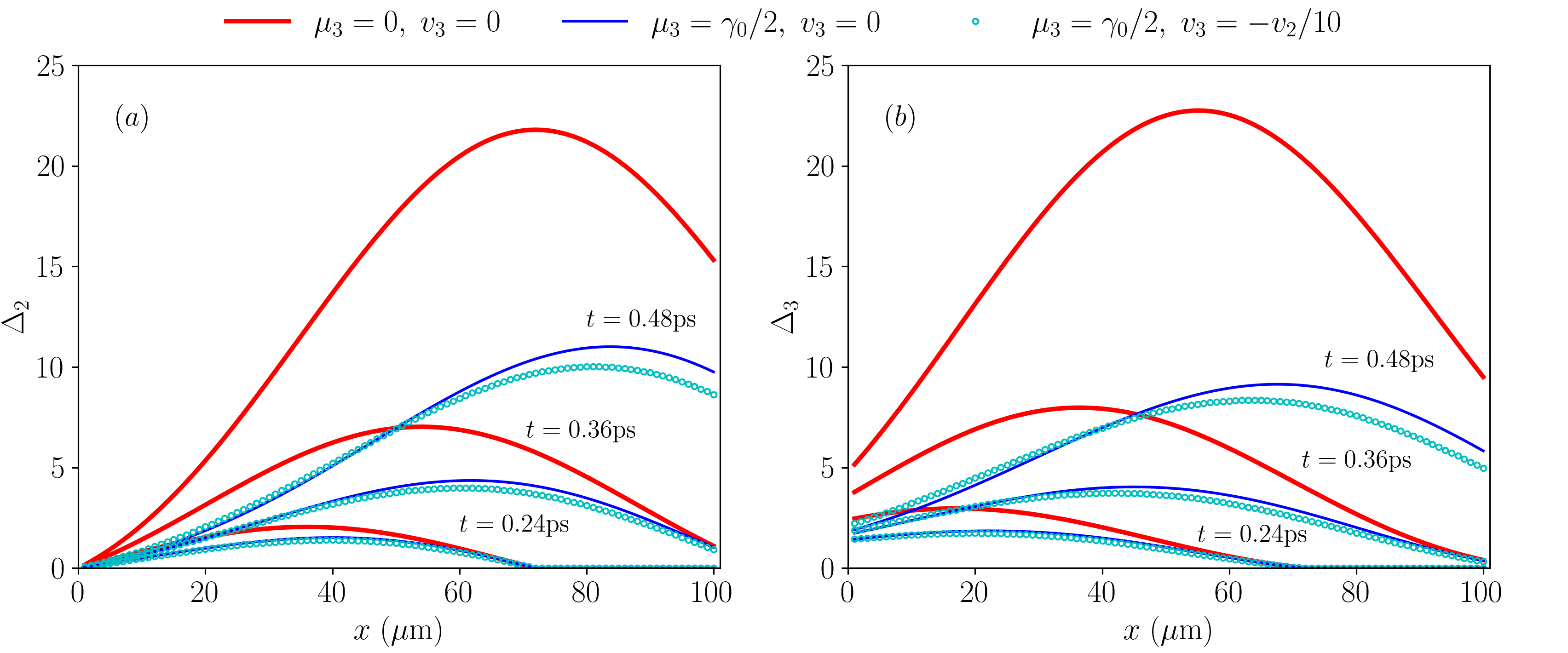
Figure 2: The growth function $\Delta_{j}(x)$ in the step-function backscattering problem for $j=2$ $(a)$ and $j=3$ $(b)$ at selected time slices when $v_{2}=3\times 10^{8}$ m/s, $\gamma_{0}=10^{13}$ rad/s, and $\mu_{2}=0$. As time increases, $\Delta_{j}$ propagates in space and grows in amplitude. The growth is always zero ahead of the wave front $x=v_{2}t$. Moreover, $\Delta_{2}(0)$ is always zero due to the boundary condition. In contrast, $\Delta_{3}(0)$ builds up from zero as time increases. Compared to the dampingless case (red lines), having an appreciable $\mu_{3}$ (blue lines) reduces the growth. Compared to the $v_{3}=0$ case (blue lines), having a small $v_{3}$ (cyan circles) slightly affects the solutions at early time. At later time, the discrepancies build up because $\gamma_{0}\approx 1.3\gamma_{a}$ exceeds the absolute instability threshold.

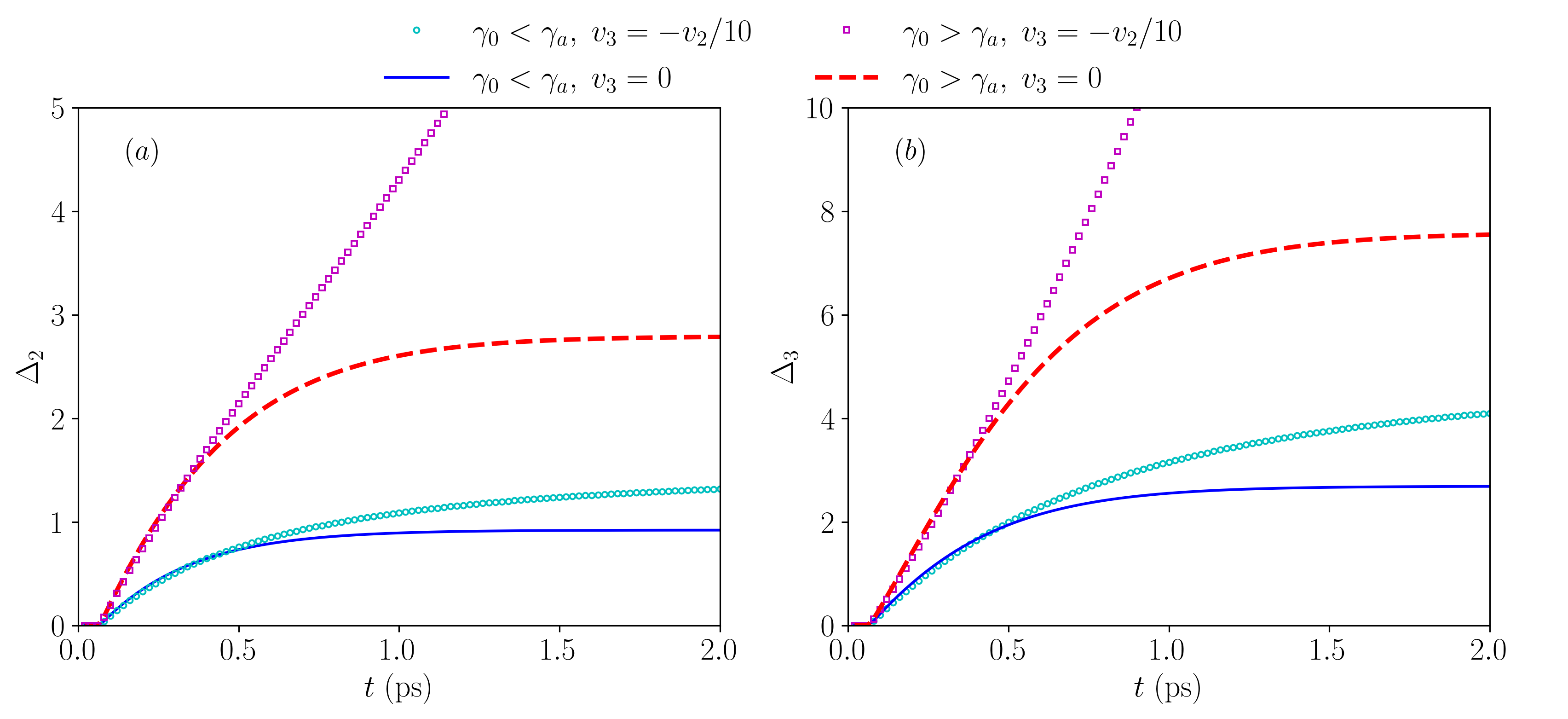
Figure 3: The growth function $\Delta_{j}(t)$ in the step-function backscattering growth problem for $j=2$ $(a)$ and $j=3$ $(b)$ at $x=20\;\mu$m when $v_{2}=3\times 10^{8}$ m/s, $\mu_{3}=5\times 10^{12}$ rad/s, and $\mu_{2}=0$. When $v_{3}=-v_{2}/10$ (symbols), the absolute instability threshold is $\gamma_{a}\approx 7.8\times 10^{12}$ rad/s. When $\gamma_{0}=7\times 10^{12}$ rad/s (cyan) is below the threshold, the growth approaches steady state. In contrary, when $\gamma_{0}=10^{13}$ rad/s (magenta) exceeds the threshold, $\Delta_{j}$ continues to increase. When $v_{3}=0$ (lines), $\gamma_{a}$ becomes infinite so the growth always saturates. The case with $\gamma_{0}=10^{13}$ rad/s (red) has a larger steady-state value than the case with $\gamma_{0}=7\times 10^{12}$ rad/s (blue). The effects of a small but finite $v_{3}$ only become significant at later time.

3 Kinetic simulations of stimulated backscattering

To benchmark the formula for magnetized three-wave coupling coefficient in the backscattering geometry, analytic solutions of the step-function problem are used to fit kinetic simulations in the same setup, where the simulations are performed using the PIC code EPOCH (arber2015contemporary). For the step-function problem, the initial condition is simply a quiescent Maxwellian plasma, whose density is chosen to be $n_{e}=n_{i}=n_{0}=$$10^{19}\;\mathrm{cm}^{-3}$ and temperature $T_{e}=T_{i}=T_{0}$ will be scanned. The two species have the mass ratio $M_{i}=m_{i}/m_{e}=1837$ of hydrogen plasmas. In the one dimensional simulation domain, the plasma occupies $x\in[0,L_{p}]$ with a constant $n_{0}$ and $T_{0}$, and two vacuum gaps each of length $L_{v}$ are placed on either side, where $L_{p}=80\lambda_{1}$, $L_{v}=10\lambda_{1}$, and $\lambda_{1}=1\,\mu$m is the vacuum pump wavelength. The slowly-varying envelope approximation requires that $L_{p}\gg\lambda_{1}$. A constant magnetic field of strength $B_{0}$ is applied in the $x$-$z$ plane at an angle $\theta_{B}$ with respect to the $x$ axis. The special case $B_{0}=0$ is unmagnetized, and the special angle $\theta_{B}=0$ means wave vectors are parallel to the magnetic field. Both $B_{0}$ and $\theta_{B}$ will be scanned.

To achieve a constant pump amplitude, the laser is launched from the right domain boundary and ramped up from zero using a $\tanh$ profile whose temporal width equals to the laser period. The smooth ramp reduces oscillations due to numerical artifacts yet is fast enough to be viewed as a step function for the slowly varying envelope. After propagating across the vacuum gap, most pump energy transmits into the plasma, and a small fraction is reflected from the plasma-vacuum boundary. The reflected pump leaves the domain from its right boundary, and the transmitted pump amplitude is measured from simulation data. Using analytical wave energy coefficient, the pump amplitude is normalized to $a_{1}$, which enters the growth rate $\gamma_{0}$ in Eq. (3). When the pump reaches the plasma-vacuum boundary on the left, most energy exists the plasma, but a small fraction is reflected. Since its wavevector is flipped, the reflected pump does not interact with the seed laser resonantly but co-propagates with the seed in $+x$ direction.

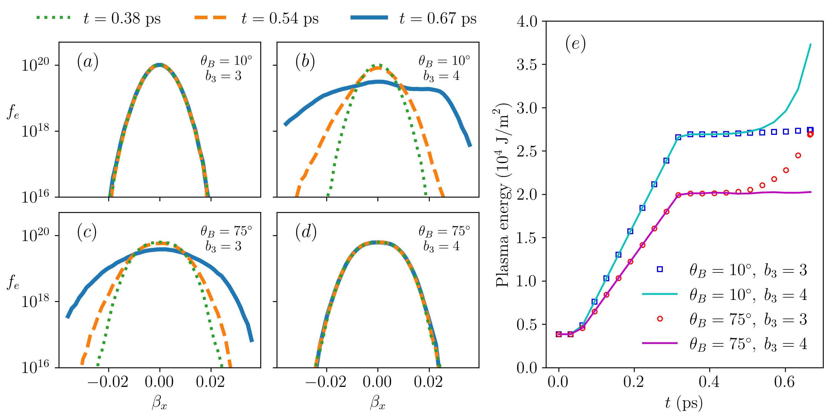
Figure 4: Plasma evolves as pump fills and seed grows. $(a)$ When $\theta_{B}=10^{\circ}$ and the coupling is weak, distribution function $f_{e}(\beta_{x})$, where $\beta_{x}=v_{x}/c$, stays near the initial Maxwellian. $(b)$ When $\theta_{B}=10^{\circ}$ but the coupling is strong, $f_{e}$ broadens rapidly. At $t=0.38$ ps (dotted green), $f_{e}$ is still close to Maxwellian, but when $t=0.54$ ps (dashed orange), non-Maxwellian tails develop. By $t=0.67$ ps (solid blue), a plateau-like structure resembles Landau damping in unmagnetized plasmas. $(c)$ When $\theta_{B}=75^{\circ}$ and the coupling is strong, $f_{e}$ also broadens significantly. In this case, $f_{e}$ remains largely symmetric due to mixing effects of gyro motion. $(d)$ When $\theta_{B}=75^{\circ}$ but the coupling is weak, $f_{e}$ barely evolves but is no longer Maxwellian due to longitudinal quiver motion in the pump laser. $(e)$ The plasma areal energy density is initially thermal $U_{T}=3T_{0}n_{0}L_{p}$$\approx 0.38\times 10^{4}\;\mathrm{J/m}^{2}$. As the pump fills in, plasma energy increases due to quiver motion. In unmagnetized plasma, $U_{Q}=\frac{1}{2}m_{e}c^{2}a_{1}^{2}n_{0}L_{p}$$\approx 2.4\times 10^{4}\;\mathrm{J/m}^{2}$. However, due to magnetization, the increase depends on $\theta_{B}$. After the seed enters, energy increases further if plasma waves are strongly excited. In these examples, $B_{0}=3$ kT, $T_{0}=10$ eV, $I_{1}=10^{15}\;\mathrm{W/cm}^{2}$, and $I_{2}=5\times 10^{12}\;\mathrm{W/cm}^{2}$. In $(a)$ and $(c)$, the interactions are mediated by F waves whose branch index is $b_{3}=3$, namely, the third highest frequency branch in warm-fluid dispersion relation. In $(b)$ and $(d)$, the interactions are mediated by P waves with $b_{3}=4$.

The seed laser $\alpha_{2}$ is launched from the left domain boundary using a similar profile but with a time delay such that its wave front enters the plasma after the pump front has existed. To measure the transmitted seed amplitude into the plasma, a seed-only run is performed to fit the boundary condition $h_{0}$ in the step-function problem. After the calibration steps, a stimulated run is performed where both the pump and seed lasers are turned on. The simulation is terminated slightly before the seed front reaches $x=L_{p}$, so that the analytical solution, which is obtained when only the left boundary is present, remains applicable. In addition, both the electron distribution function $f_{e}(v_{x})$ and the pump wave amplitude $a_{1}(x)$ are monitored during the simulations. In many cases, the change of $f_{e}$ and $a_{1}$ are small. For example, when the three-wave coupling is weak and the propagation angle $\theta_{B}$ is small (figure 4$a$), the distribution function stays close to the initial Maxwellian. In comparison, when the coupling is week but angle is close to $90^{\circ}$ (figure 4$d$), even though $f_{e}$ remains largely constant during the interaction, it is broadened from the Maxwellian due to quiver motion in the pump laser, which has an appreciable longitudinal component. The situation is different when the coupling is strong. Regardless of the angle, when a large amplitude plasma wave is excited, its collisionless damping leads to substantial broadening of $f_{e}$ as shown in figure 4$(b)$ and 4$(c)$, which correlates with a significant increase of the plasma energy (figure 4$e$) and a rapid depletion of the pump laser. The simulation data after the peak of $f_{e}$ reduces by $5\%$ or $a_{1}$ drop by $1\%$ since interactions begin are excluded from fitting, which assumes constant plasma conditions and pump amplitude.

The choice of pump and seed laser intensities are constrained by three factors. First, numerical noise of the PIC method gives an upper bound of the pump intensity due to spontaneous scattering. With a finite number of sampling particles, the plasma density fluctuates around $n_{0}$, leading to a noise $\delta E_{\parallel}$ that can spontaneously scatter the pump laser $a_{1}$. For scatterings mediated by electron modes, the growth rate is typically comparable to the cold Raman backscattering rate $\gamma_{R}=\frac{1}{2}a_{1}(\omega_{p}\omega_{1})^{1/2}$. The requirement $\gamma_{R}t_{p}\lesssim 1$ that noise does not grow substantially gives an upper bound for the pump intensity, where $t_{p}\simeq L_{p}/c$ is the time it takes for the pump to fill the plasma. Since $\gamma_{R}t_{p}=\pi(n_{0}/n_{c})^{1/4}(L_{p}/\lambda_{1})a_{1}$, where $n_{c}=\epsilon_{0}m_{e}\omega^{2}/e^{2}$ $\approx 1.1\times 10^{21}\lambda_{\mu\mathrm{m}}^{-2}\;\mathrm{cm}^{-3}$ is the critical density, we need $a_{1}\ll 10^{-1}$ with earlier choices of $n_{0}$ and $L_{p}$. In terms of laser intensity, since $a_{1}\simeq 8.6\times 10^{-3}\lambda_{\mu\mathrm{m}}I_{14}^{1/2}$, where $I_{14}$ is the intensity in units of $10^{14}\;\mathrm{W/cm}^{2}$, we see that the pump intensity cannot far exceed $I_{14}\sim 10^{2}$. Second, PIC noise also imposes a lower bound for the seed intensity. In each cell, the distribution function is sampled with $N$ super particles. Even though the mean velocity is zero, the standard error of the mean is $\delta v=v_{T}/\sqrt{N}$, where $v_{T}/c\approx 6.3\times 10^{-2}T_{\mathrm{keV}}^{1/2}$ is the electron thermal speed. The sampling error leads to a noise current density $\delta j=en_{0}\delta v$, which drives a noise field $\delta E_{\perp}=\delta j/\epsilon_{0}\omega$ at frequency $\omega$ through the Ampère’s law. In terms of the relativistic critical field $E_{c}=m_{e}\omega c/e\approx$ $3.2\times 10^{12}\lambda_{\mu\mathrm{m}}^{-1}\;\mathrm{V/m}$, the error field at the laser frequency is $\delta E_{\perp}=E_{c}(n_{0}v_{T}/n_{c}c)N^{-1/2}$$\sim 10^{7}$ V/m when $T_{0}=10$ eV and $N=10^{2}$, as shown in the inset of figure 5$(c)$. Since the laser electric field is $E=(2I/\epsilon_{0}c)^{1/2}\approx$ $2.7\times 10^{10}I_{14}^{1/2}$ V/m, the condition $E\gg\delta E_{\perp}$ requires that the seed intensity be larger than $I_{14}\sim 10^{-4}$, especially when the plasma is hotter. Finally, the pump and seed amplitudes need to be separated by about an order of magnitude. This is because in order for $a_{1}$ to remain largely constant during three-wave interactions, we need $a_{1}\gg a_{2}$. However, if $a_{1}/a_{2}$ is too large, then filtering out $a_{2}$ from simulation data becomes challenging due to leakages of $a_{1}$ through numerical filters. Combining the three constraints, intensities of pump $I_{1}$ and seed $I_{2}$ should satisfy $10^{10}\;\mathrm{W/cm}^{2}$ $\ll I_{2}\sim 10^{2}I_{1}$ and $I_{1}\ll$ $10^{16}\;\mathrm{W/cm}^{2}$. The bounds can be extended using a larger $N$. However, the benefit only increases as $\sqrt{N}$ but the numerical cost grows with $N$ linearly.

With the simulation setup and general considerations discussed above, technical details are elaborated below with examples, and the data analysis protocol is summarized in Shi22linear. All reported results use the resolution of $40$ cells per pump laser wavelength and $N=100$ particles per cell. Increasing or decreasing these parameters by a factor of two does not significantly change results. A larger plasma and simulation box increases the vulnerability to spontaneous pump scattering, which first shows up as unwanted oscillations on the right plasma boundary. On the other hand, using a much smaller plasma starts to violate $L_{p}\gg\lambda_{1}$, which is required in order for the slowly varying amplitude approximation to be valid.

3.1 Launching linear eigenmodes

Since three-wave equations describe amplitudes of linear eigenmodes, the lasers need to be launched with specified polarizations to excite targeted eigenmodes only. While polarization matching is trivial for unmagnetized plasmas, where the two electromagnetic eigenmodes are degenerate, special care needs to be taken in magnetized cases where the R and L elliptically polarized eigenmodes are nondegenerate. If the polarization is not matched properly, both R and L waves will be excited, giving rise to four polarization combinations with very different couplings (shi2019amplification). Since incident lasers are purely transverse in the vacuum region, only the perpendicular components need to be matched with plasma eigenmodes. Denoting $\psi$ the elliptical polarization angle and $\theta$ is the wave phase,

$$\mathbf{E}_{\perp}\propto\hat{\mathbf{y}}\sin\psi\sin\theta+\hat{\mathbf{k}}\times\hat{\mathbf{y}}\cos\psi\cos\theta,$$ (23)

where $\hat{\mathbf{y}}$ and $\hat{\mathbf{k}}$ are unit vectors. The expression is symmetric about the $x$-$z$ plane where $\mathbf{B}_{0}$ lies. The special value $\psi=0$ means that the wave is linearly polarized along $\hat{\mathbf{k}}\times\hat{\mathbf{y}}$, whereas $\psi=\pi/2$ means linear polarization along $\hat{\mathbf{y}}$, $\psi=\pi/4$ is R circular polarization about $\hat{\mathbf{k}}$, and $\psi=-\pi/4$ is L circular polarization.

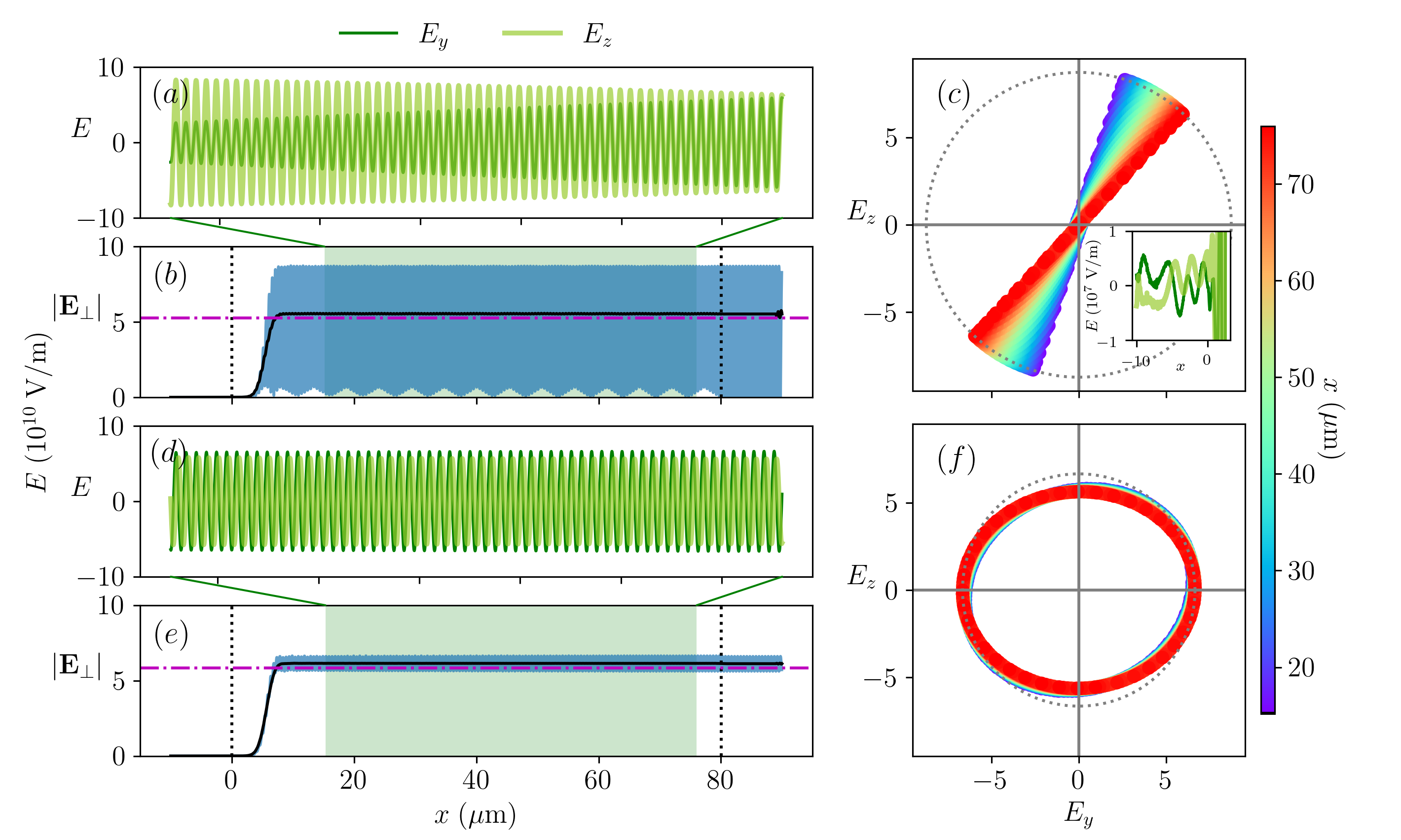
Figure 5: By launching a linearly polarized pump laser and fitting its $E_{y}$ (dark green) and $E_{z}$ (light green) components $(a)$ within the data region $(b)$, polarization angles of numerical eigenmodes can be determined. While the polarization vector slowly rotates for none eigenmodes $(c)$ as the wave propagates in $x$ (color scale), it stays close a constant ellipse $(f)$ when an eigenmode is launched, whose field components have constant amplitude $(d)$ within the data region $(e)$. The vertical dashed black lines in $(b)$ and $(e)$ mark the initial plasma-vacuum boundaries. The green shaded region is selected based on criteria that it is $4\lambda$ within the boundaries, $8\lambda$ behind the wave front, and that the $2\lambda$-running average of $|\mathbf{E}_{\perp}|$ (black) ramps above $95\%$ of its average (magenta). The inset in $(c)$ shows the noise level before the pump arrives, which is consistent with expected PIC noise when $T_{0}=10$ eV. The polarization rotation is consistent with $B_{0}=3$ kT and $\theta_{B}=30^{\circ}$. The pump intensity is $I_{1}=10^{15}\;\mathrm{W/cm}^{2}$.

Due to numerical dispersion and PIC density fluctuations, the polarization angles of numerical eigenmodes are slightly different from analytic results. Launching waves with analytical $\psi$ leads to a small but sometimes observable polarization rotation of $\mathbf{E}_{\perp}$, revealing contaminations from the unintended eigenmode. To determine $\tilde{\psi}$ for numerical eigenmodes, a calibration step is performed where a linearly polarized wave at frequency $\omega$ is launched with a constant $\mathbf{E}_{\perp}$, which lies along the diagonal of $y$-$z$ plane. In most cases, this wave has large overlaps with both numerical eigenmodes, so E_y &= E_Rsin~ψ_R sin(~k