Non-trivial class of anisotropic compact stellar model in Rastall gravity

Abstract

We investigated Rastall gravity, for an anisotropic star with a static spherical symmetry, whereas the matter-geometry coupling as assumed in Rastall Theory (RT) is expected to play a crucial role differentiating RT from General Relativity (GR). Indeed, all the obtained results confirm that RT is not equivalent to GR, however, it produces same amount of anisotropy as GR for static spherically symmetric stellar models. We used the observational constraints on the mass and the radius of the pulsar Her X-1 to determine the model parameters confirming the physical viability of the model. We found that the matter-geometry coupling in RT allows slightly less size than GR for a given mass. We confirmed the model viability via other twenty pulsars’ observations. Utilizing the strong energy condition we determined an upper bound on compactness $U_{\text{max}}\sim 0.603$, in agreement with Buchdahl limit, whereas Rastall parameter $\epsilon=-0.1$. For a surface density compatible with a neutron core at nuclear saturation density the mass-radius curve allows masses up to $3.53M_{\odot}$. We note that there is no equation of state is assumed, however the model fits well with linear behaviour. We split the twenty pulsars into four groups according to the boundary densities. Three groups are compatible with neutron cores while one group fits perfectly with higher boundary density $8\times 10^{14}$ g/cm³ which suggests that those pulsars may have quark-gluon cores.

1 Introduction

The stellar structure topic has been developed over many years either in Newtonian gravity or later in General Relativity (GR) since the firstly obtained exterior/interior solution of a spherically symmetric object Schwarzschild:1916uq ; Schwarzschild:1916ae . Motivated by the claim that pressure at core of the compact star model could have anisotropic structure where the density exceeds the nuclear density $\sim 10^{15}$ g/cm³, many models have been developed imposing the anisotropic pressure concept (assuming radial and tangential pressures are different) to derive realistic stellar models within the GR context ruderman1972pulsars (see also PhysRevD.65.104011 ; Schunck:2003kk ; Mak:2001eb ; Usov:2004iz ; Rahaman:2010mr ; Rahaman:2010bt ; Varela:2010mf ; Rahaman:2011hd ; Kalam:2012sh ; Deb:2015vda ; Shee:2015kqa ; Maurya:2016oml ) and in modified gravity as well Abbas:2014rja ; Abbas:2015yma ; Abbas:2015wea ; Zubair:2015cpa ; zubair2016some ; zubair2016possible ; Ilyas:2018tht ; Yousaf:2017lto ; Shamir:2017rjz ; Shamir:2017yza ; Das:2016mxq . Possible sources of anisotropy of ultra-compact stars could be due to solidification Palmer:1974hb , superfluidity Ramanan:2019kwf , strong magnetic fields Weber:2006ep , hyperons Rahmansyah:2020gar , pion-condesation Sawyer:1972cq and strong interactions bowers1974anisotropic . Local anisotropy and its consequences on the stability and the gravitational collapse of self-gravitating systems has been investigated by Herrera and Santos herrera1997local (see also herrera1992cracking ; Herrera:2007kz ; Herrera:2008bt ; Herrera:2011cr ).

The GR theory has been proven to be a successful theory of gravity on solar system scales (spacetime curvature is weak) by many observational tests, c.f. misner1973gravitation , and also on black hole scales (spacetime curvature is extremely strong) using black hole shadows observations by Event Horizon Telescope EventHorizonTelescope:2019dse not to mention the perfect predictions of the gravitational waves due to binary black holes merging Abbott:2016blz ; Abbott:2017oio ; TheLIGOScientific:2017qsa . On the cosmological scales, however, the GR does not provide answers for explaining the late accelerated expansion Riess:1998cb ; Perlmutter:1998np ; deBernardis:2000sbo ; Knop:2003iy . Even in presence of a cosmological constant $\Lambda$, the discrepancy of the current Hubble parameter $H_{0}$ value, between early universe observations by Planck satellite and late universe measurements by distance ladder or strong lensing, may point out the need to modify the GR theory Verde:2019ivm , see also Hashim:2020sez ; Hashim:2021pkq ; DiValentino:2021izs .

Many efforts have been done to generalize GR theory by using general function in Einstein-Hilbert action instead of the Ricci invariant, e.g. $f(R)$, $f(G)$, $f(T)$ and mimetic gravity Clifton:2011jh ; Nojiri:2006ri ; DeFelice:2010aj ; Nashed:2019tuk ; Nashed:2011fg ; 2014IJTP…53.3901W ; Nashed:2018efg ; Nashed:2020kdb ; Cognola:2006eg ; Li:2007jm ; DeFelice:2008wz ; Astashenok:2014nua ; Linder:2010py ; Cai:2015emx ; Awad:2017tyz ; Nashed:uja ; Nashed:2013bfa ; Nashed:2018qag ; Nashed:2019yto ; ElHanafy:2017sih ; Hashim:2020sez ; Hashim:2021pkq ; ElHanafy:2020pek . In fact, these modified theories kept the fundamental assumption that the covariant divergence of the energy-momentum vanishes, i.e. $\mathcal{T}^{\alpha}{{}_{\beta;\alpha}}=0$ where the semicolon denotes the Levi-Civita covariant derivative. On the contrary, Rastall attempted to modify GR by dropping this assumption replacing it by setting $\mathcal{T}^{\alpha}{{}_{\beta;\alpha}}=a_{\beta}$ where $a_{\beta}$ vanishes in flat spacetime (vacuum) and recovers GR, otherwise it does not Rastall:1972swe ; Rastall:1976uh . Rastall showed that $a_{\beta}\propto\partial_{\beta}\mathcal{R}$ is a reasonable choice which reflects the non-minimal coupling between matter and geometry. Interestingly, some cosmological models have been constructed using RT PhysRevD.85.084008 ; fabris2012rastall ; moradpour2016thermodynamics as well as black hole solutions heydarzade2017black ; ma2017noncommutative ; lobo2018thermodynamics ; bamba2018thermodynamics ; xu2018kerr . Moreover, shadows of rotating black holes have been investigated within RT by Kumar et al. kumar2018rotating and Heydarzade and Darabi heydarzade2017black . Furthermore, the effects of the non-minimal coupling between matter and geometry on thermodynamics of black holes in RT has been investigated in comparison with the GR theory lobo2018thermodynamics ; moradpour2016thermodynamic ; Soroushfar2019 ; Cruz:2019jiq .

Recently, Vissar claimed that RT is completely equivalent to GR Visser:2017gpz . On the contrary, Darabi et al. investigated Visser’s claim but they concluded that Visser misinterpreted the matter-geometry coupling term which led him to wrong conclusion Darabi:2017coc . In addition, they showed that by applying Visser’s approach to $f(R)$ theory one may conclude that it is equivalent to GR as well which is not true. Different studies have proven that RT is not equivalent to GR Hansraj:2018zwl ; Hansraj:2020clg ; abbas2018new ; abbas2018isotropic . Visser’s conclusion is correct when Ricci scalar vanishes for black holes in general, otherwise the claim is incorrect and both theories are not equivalent. One of the good examples which may reveal the contribution of the matter-geometry coupling in RT in contrast to GR is the stellar models when the presence of matter plays a crucial role. It is the aim of the present study to derive a anisotropic static spherically symmetric interior solution using RT and confront it with pulsars observations.

The arrangement of this study is as follows: In Section 2 we briefly review the main assumptions and features of the non-conservative theory of Rastall’s gravity. In Section 3, we apply Rastall’s field equations to a spherically symmetrical object in presence of anisotropic matter source. The system consists of three non-linear differential equations in five unknown functions (two metric potentials in addition to the energy-density, radial and tangential pressures). Therefore, two constraints have been imposed to close the system without using equation of state (EoS): We assumed a specific form of one of the metric potential, $g_{rr}$ as usually done in interior solutions, additionally we made the metric potential $g_{tt}$ contribution to the anisotropy to vanish. Consequently, we derive the analytic form of energy-density, radial, and tangential pressures which satisfy Rastall field equations. In Section 4, we list the necessary and sufficient physical conditions that any stellar model must fulfill to be compatible with a realistic compact star. In Section 5, we investigated the viability of the obtained solution with the conditions listed in Section 4. In Section 6, we matched our model with the exterior vacuum solution (Schwarzschild solution) fixing the model parameters and constants. The pulsar Her X-1 , with mass $M=0.85\pm 0.15\,M_{\odot},$ and radius $R=8.1\pm 0.41$ km Abubekerov_2008 is used to determine the constants of the model. In Section 7, we investigated the stability of the model using a modified version of Tolman-Oppenheimer-Volkoff (TOV) equation of hydrostatic equilibrium and the adiabatic indices. In Section 8 we use other observational mass-radius constraints of twenty pulsars’ data to test the viability of the model. Also we plot the mass-radius profile of the model for different surface densities compatible with neutron core pulsars to show the maximum masses allowed by the model. Finally, we summarize and conclude in Section 9.

2 Rastall gravitational theory

In Riemann geometry, by making use of the contracted Bianchi Identity on one hand and the minimal coupling procedure on the other hand,

$$\mathcal{G}_{\alpha\beta;\alpha}=(\mathcal{R}_{\alpha\beta}-\frac{1}{2}g_{\alpha\beta}\mathcal{R})_{;\alpha}\equiv 0,\qquad\qquad\mathcal{T}_{\alpha\beta;\alpha}=0,$$ (1)

this led Einstein to formulate the consistent field equations of GR

$$\mathcal{G}_{\alpha\beta}=\chi\mathcal{T}_{\alpha\beta},$$ (2)

where $\chi=8\pi G_{N}/c^{4}$ where $G_{N}$ is the Newtonian gravitational constant and $c$ is the speed of light, $\mathcal{G}_{\alpha\beta}$ denotes Einstein tensor, $\mathcal{R}_{\alpha\beta}$ denotes Ricci tensor and $\mathcal{R}=g^{\alpha\beta}\mathcal{R}_{\alpha\beta}$ denotes Ricci invariant. Rastall, however, dropped the minimal coupling procedure assuming non-divergence-free energy-momentum in curved spacetime Rastall:1972swe ; Rastall:1976uh

$$\mathcal{T}^{\alpha}{}_{\beta;\alpha}\neq 0,\qquad\mathcal{T}^{\alpha}{}_{\beta;\alpha}=a_{\beta}=\tilde{\epsilon}\,\partial_{\beta}\mathcal{R},$$ (3)

where the constant of proportionality $\tilde{\epsilon}$ measures how much the conservation law is locally violated. According to this assumption Rastall obtained a consistent set of field equations

$$\mathcal{G}_{\alpha\beta}=\mathcal{R}_{\alpha\beta}-\frac{1}{2}g_{\alpha\beta}\mathcal{R}=\chi(\mathcal{T}_{\alpha\beta}-\tilde{\epsilon}g_{\alpha\beta}\mathcal{R}).$$ (4)

Obviously Rastall gravity reflects non-minimal coupling features of matter and geometry whereas Einstein’s field equations are recovered when the spacetime is flat. Alternatively, Eq. (4) can be rewritten as

$$\mathcal{R}_{\alpha\beta}-\left(\frac{1}{2}-\chi\tilde{\epsilon}\right)g_{\alpha\beta}\mathcal{R}=\chi\mathcal{T}_{\alpha\beta}.$$ (5)

Contracting the above equation gives

$$(1-4\chi\tilde{\epsilon})\mathcal{R}=-\chi\mathcal{T},$$ (6)

where $\mathcal{T}=g^{\alpha\beta}\mathcal{T}_{\alpha\beta}$ is the trace of the energy-momentum tensor. Thus the field equations of RT read

$$\mathcal{G}_{\alpha\beta}=\chi\widetilde{\mathcal{T}}_{\alpha\beta}.$$ (7)

where

$$\widetilde{\mathcal{T}}_{\alpha\beta}=\mathcal{T}_{\alpha\beta}+\frac{\chi\tilde{\epsilon}}{1-4\chi\tilde{\epsilon}}g_{\alpha\beta}\mathcal{T},\qquad 1-4\chi\tilde{\epsilon}\neq 0.$$ (8)

It proves convenient to use a dimensionless Rastall’s parameter $\epsilon=\tilde{\epsilon}\chi$, c.f. Oliveira:2015lka . Then, Eq. (5) becomes

$$\mathcal{R}_{\alpha\beta}-\left(\frac{1}{2}-\epsilon\right){g}_{\alpha\beta}\mathcal{R}=\chi\mathcal{T}_{\alpha\beta},$$ (9)

and the tensor $\widetilde{\mathcal{T}}_{\alpha\beta}$ in Eq. (7) reads

$$\widetilde{\mathcal{T}}_{\alpha\beta}=\mathcal{T}_{\alpha\beta}+\frac{\epsilon}{1-4\epsilon}g_{\alpha\beta}\mathcal{T},\qquad\epsilon\neq\frac{1}{4}.$$ (10)

For $\epsilon=0$ case, the conservation law is restored and the GR version of gravity is recovered. In this sense, RT generalizes Einstein’s one by assuming a local violation of conservation law in curved spacetime due to non-minimal coupling between matter and geometry. Otherwise, flat spacetime, both theories are equivalent. Therefore, one of the important applications, which differentiate both theories, is stellar structure models when presence of the matter sector plays a crucial role in interior solutions.

3 spherically symmetric interior solution

Providing that the static spherically symmetrical spacetime is given by the following metric

$$ds^{2}=-F(r)dt^{2}+G(r)\,dr^{2}+r^{2}(d\theta^{2}+\sin^{2}{\theta}\,d\phi^{2})\,,$$ (11)

where $F(r)$ and $G(r)$ are unknown functions. For the spacetime metric (11), we obtain the non-vanishing components of Levi-Civita connection

$${\Gamma_{tt}}^{r}=\frac{F^{\prime}}{2G}\,,\qquad\qquad{\Gamma_{tr}}^{t}=\frac{F^{\prime}}{2F}\,,\qquad\qquad{\Gamma_{rr}}^{r}=\frac{G^{\prime}}{2G}\,,\qquad\qquad{\Gamma_{r\theta}}^{\theta}={\Gamma_{r\phi}}^{\phi}=\frac{1}{r}\,,$$

$${\Gamma_{\theta\theta}}^{r}=-\frac{r}{G}\,,\qquad\qquad{\Gamma_{\theta\phi}}^{\phi}=\cot\theta\,,\qquad\qquad{\Gamma_{\phi\phi}}^{r}=-\frac{r\sin^{2}\theta}{G}\,,\qquad\qquad{\Gamma_{\phi\phi}}^{\theta}=-\sin\theta\,\cos\theta\,,$$ (12)

where prime (double prime) denotes first (second) derivative with respect to the radial coordinate. We write the Ricci invariant

$$\mathcal{R}(r)={-2F^{\prime\prime}GFr^{2}+F^{\prime 2}Gr^{2}+rFF^{\prime}(rG^{\prime}-4G)+4F^{2}[rG^{\prime}+G(G-1)]\over 2F^{2}G^{2}r^{2}}\,.$$ (13)

We assume the energy-momentum tensor for a anisotropic fluid with spherical symmetry, i.e.

$$\mathcal{T}{{}^{\alpha}}{{}_{\beta}}=(p_{t}+\rho)u{{}^{\alpha}}u{{}_{\beta}}+p_{t}\delta^{\alpha}_{\beta}+(p_{r}-p_{t})\zeta{{}^{\alpha}}\zeta{{}_{\beta}},$$ (14)

where $\rho=\rho(r)$ is the fluid energy density, $p_{r}=p_{r}(r)$ its radial pressure (in the direction the time-like four-velocity $u_{\alpha}$), $p_{t}=p_{t}(r)$ its tangential pressure (perpendicular to $u_{\alpha}$) and $\zeta{{}^{\alpha}}$ is the unit space-like vector in the radial direction. Then, the energy-momentum tensor takes the diagonal form $\mathcal{T}{{}^{\alpha}}{{}_{\beta}}=diag(-\rho,\,p_{r},\,p_{t},\,p_{t})$.

Applying Rastall’s field equations (7) to the spacetime (11) where the matter sector is as given by (14) we obtain, respectively, the components $t\,t$, $r\,r$ and $\theta\,\theta$ ($=\phi\,\phi$) as follows:

$$\rho = {rG^{\prime}+G(G-1)\over G^{2}r^{2}}-{\epsilon\over 1-4\epsilon}(\rho-p_{r}-2p_{t})\,,$$

$$p_{r} = {F^{\prime}r-F(G-1)\over FGr^{2}}+{\epsilon\over 1-4\epsilon}(\rho-p_{r}-2p_{t})\,,$$

$$p_{t} = {F[2G(F^{\prime\prime}r+F^{\prime})-G^{\prime}F^{\prime}r]-2G^{\prime}F^{2}-F^{\prime 2}Gr\over 4F^{2}G^{2}r}+{\epsilon\over 1-4\epsilon}(\rho-p_{r}-2p_{t})\,.$$ (15)

Additionally, we define the anisotropy of the system (15) using the parameter

$$\Delta(r)=p_{t}-p_{r}={2F^{\prime\prime}GFr^{2}-F^{\prime 2}Gr^{2}-rFF^{\prime}(rG^{\prime}+2G)-2F^{2}[rG^{\prime}-2G(G-1)]\over 4F^{2}G^{2}r^{2}}\,.$$ (16)

We note that the Rastall parameter quantitatively contributes in the radial and the tangential pressures by equal amount, i.e. Rastall parameter has no contribution in the anisotropy parameter, and this conclusion is valid for any spherically symmetric interior solution. For the $\epsilon=0$ case, the differential equations (15) coincide with Einstein field equations of an interior spherically symmetrical spacetime Nashed:2020buf ; Nashed:2020kjh . The system (15) consists of three independent non-linear differential equations in five unknowns $G$, $F$, $\rho$, $p_{r}$ and $p_{t}$. Therefore, two conditions need to be imposed to close the above system. We follow the ansatz given in Das:2019dkn (also used in Nashed:2020kjh ). First, we assume the metric potential $G$ to have the form

$$G(r)=\frac{1}{\left(1-\frac{a_{2}^{2}r^{2}}{R^{2}}\right)^{4}}\,,$$ (17)

with $a_{2}$ is a dimensionless constant to be determined by boundary condition and $R$ is the radius at the star boundary. We note that the above ansatz is regular everywhere inside the star, i.e. $0\leq r\leq R$, where $|a_{2}|<1$. Substituting (17) in the anisotropy parameter (16), we get

$$\Delta(r)={a_{2}^{4}r^{2}(6R^{4}-8R^{2}a_{2}^{2}r^{2}+3a_{2}^{4}r^{4})\over R^{8}}+{{(R^{2}-a_{2}^{2}r^{2})^{3}}[r(2FF^{\prime\prime}-F^{\prime 2})(R^{2}-a_{2}^{2}r^{2})-2FF^{\prime}(R^{2}+3a_{2}^{2}r^{2})]\over 4rF^{2}R^{8}}\,.$$ (18)

Now, we impose the second condition by assuming that the component $g_{tt}$ has no contribution on the anisotropy parameter, i.e.

$$\Delta(r)={a_{2}^{4}r^{2}(6R^{4}-8R^{2}a_{2}^{2}r^{2}+3a_{2}^{4}r^{4})\over R^{8}}\,.$$ (19)

This choice clearly gives no anisotropy at the center, $r=0$, which is physically a reasonable feature Das:2019dkn , see the physical conditions in Sec. 4. Using Eqs. (18) and (19) and by solving for the metric potential $F$, we obtain:

$$F(r)={[a_{0}R^{2}+2a_{1}a_{2}^{2}(R^{2}-a_{2}^{2}r^{2})]^{2}\over 8a_{2}^{4}(R^{2}-a_{2}^{2}r^{2})^{2}}\,,$$ (20)

where the constants of integration $a_{0}$ and $a_{1}$ are dimensionless to be fixed by matching conditions. Up to this step the obtained results are the same as given by Das:2019dkn . However, the matching conditions with the exterior solution give the set of constants {$a_{0}$, $a_{1}$, $a_{2}$} in terms of Rastall parameter $\epsilon$. Therefore, any deviation from the GR in the following results should be related to the assumed matter-geometry coupling in Rastall field equations (15), i.e. Rastall parameter $\epsilon$.

Substituting the metric potentials (17) and (20) into the system (15), we get the energy-density, radial and tangential pressures in the form

$$\rho = \frac{12a_{2}^{2}}{R^{8}[2a_{1}a_{2}^{2}(a_{2}^{2}r^{2}-R^{2})-a_{0}R^{2}]}\Bigg{\{}{\frac{3a_{1}a_{2}^{10}}{2}(2\epsilon-1)}r^{8}-\frac{a_{2}^{6}}{2}{\left[\frac{a_{1}a_{2}^{2}}{3}(74\epsilon-37)+\frac{a_{0}}{2}(2\epsilon-3)\right]}R^{2}r^{6}$$

$$+\frac{a_{2}^{4}}{3}{\left[a_{1}a_{2}^{2}(58\epsilon-29)+a_{0}(5\epsilon-7)\right]}R^{4}r^{4}-2a_{2}^{2}{\left[\frac{7a_{1}a_{2}^{2}}{2}(2\epsilon-1)+\frac{a_{0}}{4}(4\epsilon-5)\right]}R^{6}r^{2}+{\left[(4a_{1}a_{2}^{2}+a_{0})\epsilon-(2a_{1}a_{2}^{2}+a_{0})\right]}R^{8}\Bigg{\}}\,,$$

$$p_{r} = \frac{12a_{2}^{2}}{R^{8}[2a_{1}a_{2}^{2}(R^{2}-a_{2}^{2}r^{2})+a_{0}R^{2}]}\Bigg{\{}{\frac{a_{1}a_{2}^{10}}{6}(18\epsilon-1)}r^{8}-\frac{a_{2}^{6}}{2}{\left[\frac{a_{1}a_{2}^{2}}{3}(74\epsilon-5)+\frac{a_{0}}{2}(2\epsilon+1)\right]}R^{2}r^{6}$$

$$+\frac{a_{2}^{4}}{3}{\left[a_{1}a_{2}^{2}(58\epsilon-5)+a_{0}(5\epsilon+2)\right]}R^{4}r^{4}-2a_{2}^{2}{\left[\frac{a_{1}a_{2}^{2}}{6}(42\epsilon-5)+\frac{a_{0}}{4}(4\epsilon+1)\right]}R^{6}r^{2}+{\left[(4a_{1}a_{2}^{2}+a_{0})\epsilon-\frac{2}{3}a_{1}a_{2}^{2}\right]}R^{8}\Bigg{\}}\,,$$

$$p_{t} = \frac{12a_{2}^{2}}{R^{8}[2a_{1}a_{2}^{2}(R^{2}-a_{2}^{2}r^{2})+a_{0}R^{2}]}\Bigg{\{}{\frac{a_{1}a_{2}^{10}}{3}(9\epsilon-2)}r^{8}-\frac{a_{2}^{6}}{2}{\left[\frac{2a_{1}a_{2}^{2}}{3}(74\epsilon-8)+a_{0}\epsilon\right]}R^{2}r^{6}+\frac{a_{2}^{4}}{3}{\left[a_{1}a_{2}^{2}(58\epsilon-12)+5a_{0}\epsilon\right]}R^{4}r^{4}$$ (21)

$$-2a_{2}^{2}{\left[\frac{a_{1}a_{2}^{2}}{3}(42\epsilon-4)+a_{0}\epsilon\right]}R^{6}r^{2}+{\left[(4a_{1}a_{2}^{2}+a_{0})\epsilon-\frac{2}{3}a_{1}a_{2}^{2}\right]}R^{8}\Bigg{\}}\,,$$

Equations (3) coincide with the GR version when Rastall parameter $\epsilon$ vanishes Nashed:2020buf . It is to be mentioned that the anisotropic force, $F_{a}=\frac{2\Delta}{r}$, becomes attractive if $p_{t}-p_{r}<0$ and repulsive if $p_{t}-p_{r}>0$. The mass contained within a radius $r$ of the sphere is defined as

$$M(r)=4\pi\int_{0}^{r}\rho(\zeta)\zeta^{2}d\zeta\,.$$ (22)

Using the energy-density as defined in Eqs. (3) and the above equation (22), we get

$$M(r)=\frac{-3\pi}{a_{1}^{4}a_{2}^{10}R^{8}\aleph}\Bigg{\{}\frac{\sqrt{2}a_{0}R^{9}\epsilon}{2}(a_{0}+2a_{1}a_{2}^{2})\tanh^{-1}\left(\frac{\sqrt{2}a_{1}a_{2}^{2}r}{R\aleph}\right)+a_{2}^{2}\aleph r\left[\frac{256a_{1}^{4}a_{2}^{10}r^{2}}{3}(2\epsilon-1)\left(2R^{2}-a_{2}^{2}r^{2}\right)\left(2R^{4}+\right.\right.$$

$$\left.\left.a_{2}^{4}r^{4}-2a_{2}^{2}R^{2}r^{2}\right)+a_{0}R^{2}\epsilon\left(a_{0}^{3}R^{6}+\frac{2r^{2}a_{1}a_{2}^{4}}{8}(4a_{1}^{2}a_{2}^{4}-2a_{1}a_{2}^{2}a_{0}+a_{0}^{2})R^{4}+\frac{4a_{1}^{2}a_{2}^{8}r^{4}}{5}(a_{0}-4a_{1}a_{2}^{2})R^{2}+\frac{8a_{1}^{3}a_{2}^{12}r^{6}}{7}\right)\right]\Bigg{\}},\qquad$$ (23)

where $\aleph=\sqrt{(a_{0}+2a_{1}a_{2}^{2})a_{1}}$. It proves convenient to use the compactness parameter Singh:2019ykp ; Roupas:2020mvs of a spherically symmetric source with radius $r$,

$$u(r)=\frac{2M(r)}{r},$$ (24)

to study the stability of compact objects. Similarly we use the gravitational red-shift parameter $Z$ which is related to the metric potential as

$$1+Z=\frac{1}{\sqrt{-g_{tt}}}.$$ (25)

These parameters will be used later in Sec 6. In the next section, however, we are going to discuss the physical requirements to derive viable stellar structures in order to test the viability of the obtained model.

4 Physical conditions for a stellar model

For a stellar model to be physically well behaved, it needs to satisfy the following conditions:
(i) For the geometric sector, the metric potentials $F$ and $G$ should be free from coordinate and physical singularities within the interior region of the star $0\leq r\leq R$, where the center (boundary) is at $r=0$ ($r=R$) respectively.

(ii) The metric potentials of the interior solution and the exterior should match smoothly at the boundary.

(iii) For the matter sector, the fluid density, radial and the tangential pressures should be free from coordinate or physical singularities within the interior region of the star. In addition, they should be maximum at the center of the star and monotonically decrease towards the boundary of the star. i.e.

• $\rho(r=0)>0$, $\rho^{\prime}(r=0)=0$, $\rho^{\prime\prime}(r=0)<0$ and $\rho^{\prime}(0<r\leq R)<0$,

• $p_{r}(r=0)>0$, $p_{r}^{\prime}(r=0)=0$, $p_{r}^{\prime\prime}(r=0)<0$ and $p_{r}^{\prime}(0<r\leq R)<0$,

• $p_{t}(r=0)>0$, $p_{t}^{\prime}(r=0)=0$, $p_{t}^{\prime\prime}(r=0)<0$ and $p_{t}^{\prime}(0<r\leq R)<0$.
  

(iv) At the center of the star ($r=0$), the anisotropy parameter $\Delta$ should vanish, i.e. $p_{r}(r=0)=p_{t}(r=0)$, and increasing toward the boundary, i.e. $\Delta^{\prime}(0\leq r\leq R)>0$.

(v) At the boundary of the star ($r=R$), the radial pressure should vanish, i.e. $p_{r}(r=R)=0$. However, the tangential pressure at the boundary should not necessarily vanish.

(vi) Within the star ($0<r<R$), the density, radial and tangential pressures should be positive, i.e. $\rho(0<r<R)>0$, $p_{r}(0<r<R)>0$ and $p_{t}(0<r<R)>0$.

(vii) The fluid density, radial and tangential pressures should fulfill the following energy conditions:

• Null energy condition (NEC): $\rho c^{2}+p_{t}>0$, $\rho>0$,

• Weak energy condition (WEC): $\rho c^{2}+p_{r}>0$, $\rho>0$,

• Dominant energy conditions (DEC): $\rho c^{2}\geq\lvert p_{r}\lvert$ and $\rho c^{2}\geq\lvert p_{t}\lvert$,

• Strong energy condition (SEC): $\rho c^{2}+p_{r}>0$, $\rho c^{2}+p_{t}>0$, $\rho c^{2}-p_{r}-2p_{t}>0$.
  

(viii) The causality condition should be satisfied, that is the speed of sound should be smaller than unity everywhere inside the star and monotonically decrease toward the boundary, i.e. for the radial velocity $0\leq v_{r}/c=\frac{1}{c}\sqrt{\frac{dp_{r}}{d\rho}}\leq 1$ and $v^{\prime}_{r}{{}^{2}}<0$, and for the tangential velocity $0\leq v_{t}/c=\frac{1}{c}\sqrt{\frac{dp_{t}}{d\rho}}\leq 1$ and $v^{\prime}_{t}{{}^{2}}<0$.

(ix) The stability condition should be satisfied, i.e. $-1<(v_{t}^{2}-v_{r}^{2})/c^{2}<0$ within the star HERRERa1992206 .

(x) The gravitational red-shift should be finite and positive everywhere inside the star and decreases monotonically toward the boundary, i.e. $Z>0$ and $Z^{\prime}<0$.

(xi) The adiabatic index stability condition for anisotropic star should be fulfilled, i.e. the adiabatic index $\Gamma>\gamma$ where $\gamma=4/3$ is the adiabatic index corresponds to the isotropic case.

We note that the stellar model which fulfills the above mentioned conditions is physically viable and well behaved. In the following sections we are going to examine the model at hand with these conditions investigating possible roles of Rastall parameter.

5 Physical properties of the model

We test the model showing that the metric potentials (17) and (20), and the solution (3) are free from physical or geometric singularities. Then we derive some physical quantities which will be used later in Sec. 6 to examine the viability of the present model. In addition, we use the matching conditions at the boundary surface of the star to set the constraining equations on the model parameters {$\epsilon,a_{0},a_{1},a_{2}$}.

5.1 Non singular model

From Eqs. (17) and (20) one finds that the metric potentials at the center read

$$F(r=0)={(a_{0}+2a_{1}a_{2}^{2})^{2}\over 16a_{2}^{4}}\,\qquad\qquad\textrm{and}\qquad\qquad G(r=0)=1.$$ (26)

This ensures that the gravitational potentials are finite at the center of the star. Moreover, the derivatives of these potentials are finite at the center, i.e. $F^{\prime}(r=0)=G^{\prime}(r=0)=0$. Equation (26) ensures that the metric is regular at the center. This satisfies condition (i) in Sec. 4.

From Eqs. (3) one finds that the density, radial and tangential pressures at the center are

$$\rho(r=0)={-12a_{2}^{2}[a_{0}(\epsilon-1)+2a_{1}a_{2}^{2}(2\epsilon-1)]\over R^{2}(a_{0}+2a_{1}a_{2}^{2})}\,,\qquad p_{r}(r=0)=p_{t}(r=0)={12a_{2}^{2}[a_{0}\epsilon+\frac{2}{3}a_{1}a_{2}^{2}(6\epsilon-1)]\over R^{2}(a_{0}+2a_{1}a_{2}^{2})}.$$ (27)

These ensure that the anisotropy parameter has a vanishing value at the center as stated in condition (iv) on Sec. 4. The density and the pressures should be positive at the center which sets two constraints on the model parameters/constants. Additionally, the Zeldovich condition 1971reas.book…..Z states that the radial pressure must be less than or equal to the density at the center, i.e. $\frac{p_{r}(0)}{\rho(0)}\leq 1$, i.e.

$${-3(a_{0}+4a_{1}a_{2}^{2})\epsilon+2a_{1}a_{2}^{2}\over 3(a_{0}+4a_{1}a_{2}^{2})\epsilon-3(a_{0}+2a_{1}a2^{2})}\leq 1.$$ (28)

Using Eqs. (3) we give the derivative of energy density, radial and tangential pressures, respectively, as follows

$$\rho^{\prime} = \frac{2r{a_{2}}^{4}}{{R}^{8}\left(a_{0}{R}^{2}+2\,a_{1}{a_{2}}^{2}{R}^{2}-2a_{1}{a_{2}}^{4}{r}^{2}\right)^{2}}\biggl{\{}216{r}^{8}{a_{1}}^{2}{a_{2}}^{12}\epsilon-108\,{r}^{8}{a_{1}}^{2}{a_{2}}^{12}+440{r}^{6}{R}^{2}{a_{1}}^{2}{a_{2}}^{10}-880{r}^{6}{R}^{2}{a_{1}}^{2}{a_{2}}^{10}\epsilon$$ (29)

$$-676\,{r}^{4}{R}^{4}{a_{1}}^{2}{a_{2}}^{8}+1352\,{r}^{4}{R}^{4}{a_{1}}^{2}{a_{2}}^{8}\epsilon-168\,{r}^{6}{R}^{2}a_{1}\,{a_{2}}^{8}a_{0}\,\epsilon+108\,{r}^{6}{R}^{2}a_{1}\,{a_{2}}^{8}a_{0}+464\,{r}^{2}{R}^{6}{a_{1}}^{2}{a_{2}}^{6}-928\,{r}^{2}{R}^{6}{a_{1}}^{2}{a_{2}}^{6}\epsilon$$

$$+520\,{r}^{4}{R}^{4}a_{1}\,{a_{2}}^{6}a_{0}\,\epsilon-332\,{r}^{4}{R}^{4}a_{1}\,{a_{2}}^{6}a_{0}-120\,{R}^{8}{a_{2}}^{4}{a_{1}}^{2}+240\,{R}^{8}{a_{2}}^{4}{a_{1}}^{2}\epsilon-544\,x{R}^{6}{a_{2}}^{4}{r}^{2}a_{0}\,a_{1}\,\epsilon+344\,{R}^{6}{a_{2}}^{4}{r}^{2}a_{0}\,a_{1}$$

$$-27\,{R}^{4}{a_{2}}^{4}{r}^{4}{a_{0}}^{2}+18\,{R}^{4}{a_{2}}^{4}{r}^{4}{a_{0}}^{2}\epsilon-120\,a_{0}\,{R}^{8}{a_{2}}^{2}a_{1}+192\,a_{0}\,{R}^{8}{a_{2}}^{2}a_{1}\,\epsilon+56\,{a_{0}}^{2}{R}^{6}{a_{2}}^{2}{r}^{2}-40\,{a_{0}}^{2}{R}^{6}{a_{2}}^{2}{r}^{2}\epsilon-30\,{a_{0}}^{2}{R}^{8}$$

$$+24\,{a_{0}}^{2}{R}^{8}\epsilon\biggr{\}}\,,$$

$$p^{\prime}_{r} = \frac{-2r{a_{2}}^{4}}{{R}^{8}\left(a_{0}\,{R}^{2}+2\,a_{1}\,{a_{2}}^{2}{R}^{2}-2\,a_{1}\,{a_{2}}^{4}{r}^{2}\right)^{2}}\biggl{\{}216\,{r}^{8}{a_{1}}^{2}{a_{2}}^{12}\epsilon-12\,{r}^{8}{a_{1}}^{2}a_{2}^{12}+56\,{r}^{6}{R}^{2}{a_{1}}^{2}{a_{2}}^{10}-880\,{r}^{6}{R}^{2}{a_{1}}^{2}{a_{2}}^{10}\epsilon$$ (30)

$$+1352\,{r}^{4}{R}^{4}{a_{1}}^{2}{a_{2}}^{8}\epsilon-100\,{r}^{4}{R}^{4}{a_{1}}^{2}{a_{2}}^{8}-168\,{r}^{6}{R}^{2}a_{1}\,{a_{2}}^{8}a_{0}\,\epsilon-4\,{r}^{6}{R}^{2}a_{1}\,{a_{2}}^{8}a_{0}+80\,{r}^{2}{R}^{6}{a_{1}}^{2}{a_{2}}^{6}-928\,{r}^{2}{R}^{6}{a_{1}}^{2}{a_{2}}^{6}\epsilon$$

$$+520\,{r}^{4}{R}^{4}a_{1}\,{a_{2}}^{6}a_{0}\,\epsilon+4\,{r}^{4}{R}^{4}a_{1}\,{a_{2}}^{6}a_{0}+240\,{R}^{8}{a_{2}}^{4}{a_{1}}^{2}\epsilon-24\,{R}^{8}{a_{2}}^{4}{a_{1}}^{2}-544\,{R}^{6}{a_{2}}^{4}{r}^{2}a_{0}\,a_{1}\,\epsilon+8\,{R}^{6}{a_{2}}^{4}{r}^{2}a_{0}\,a_{1}$$

$$+9\,{R}^{4}{a_{2}}^{4}{r}^{4}{a_{0}}^{2}+18\,{R}^{4}{a_{2}}^{4}{r}^{4}{a_{0}}^{2}\epsilon-8\,a_{0}\,{R}^{8}{a_{2}}^{2}a_{1}+192\,a_{0}\,{R}^{8}{a_{2}}^{2}a_{1}\,\epsilon-16\,{a_{0}}^{2}{R}^{6}{a_{2}}^{2}{r}^{2}-40\,{a_{0}}^{2}{R}^{6}{a_{2}}^{2}{r}^{2}\epsilon+6\,{a_{0}}^{2}{R}^{8}$$

$$+24\,{a_{0}}^{2}{R}^{8}\epsilon\biggr{\}}\,,$$

$$p^{\prime}_{t} = \frac{-4r{a_{2}}^{4}}{{R}^{8}\left(a_{0}{R}^{2}+2a_{1}{a_{2}}^{2}{R}^{2}-2a_{1}{a_{2}}^{4}{r}^{2}\right)^{2}}\biggl{\{}108{r}^{8}{a_{1}}^{2}{a_{2}}^{12}\epsilon-24{r}^{8}{a_{1}}^{2}{a_{2}}^{12}+96{r}^{6}{R}^{2}{a_{1}}^{2}{a_{2}}^{10}-440{r}^{6}{R}^{2}{a_{1}}^{2}{a_{2}}^{10}\epsilon-144{r}^{4}{R}^{4}{a_{1}}^{2}{a_{2}}^{8}$$ (31)

$$+676{r}^{4}{R}^{4}{a_{1}}^{2}{a_{2}}^{8}\epsilon-84{r}^{6}{R}^{2}a_{1}{a_{2}}^{8}a_{0}\epsilon+16{r}^{6}{R}^{2}a_{1}{a_{2}}^{8}a_{0}-464{r}^{2}{R}^{6}{a_{1}}^{2}{a_{2}}^{6}\epsilon+96{r}^{2}{R}^{6}{a_{1}}^{2}{a_{2}}^{6}+260{r}^{4}{R}^{4}a_{1}{a_{2}}^{6}a_{0}\epsilon+12{a_{0}}^{2}{R}^{8}\epsilon$$

$$-48\,{r}^{4}{R}^{4}a_{1}\,{a_{2}}^{6}a_{0}-24\,{R}^{8}{a_{2}}^{4}{a_{1}}^{2}+120\,{R}^{8}{a_{2}}^{4}{a_{1}}^{2}\epsilon-272\,{R}^{6}{a_{2}}^{4}{r}^{2}a_{0}\,a_{1}\,\epsilon+48\,{R}^{6}{a_{2}}^{4}{r}^{2}a_{0}\,a_{1}+9\,{R}^{4}{a_{2}}^{4}{r}^{4}{a_{0}}^{2}\epsilon-16\,a_{0}\,{R}^{8}{a_{2}}^{2}a_{1}$$

$$+96\,a_{0}\,{R}^{8}{a_{2}}^{2}a_{1}\,\epsilon-20\,{a_{0}}^{2}{R}^{6}{a_{2}}^{2}{r}^{2}\epsilon\biggr{\}}\,.$$

We use Eqs. (29)–(31) to show that the gradients of the energy-density, radial and tangential pressures are negative later in Sec. 6.

The radial and tangential sound velocities are given

$$v_{r}^{2} = \frac{dp_{r}}{d\rho}=-\biggl{\{}216\,{r}^{8}{a_{1}}^{2}{a_{2}}^{12}\epsilon-12\,{r}^{8}{a_{1}}^{2}{a_{2}}^{12}+56\,{r}^{6}{R}^{2}{a_{1}}^{2}{a_{2}}^{10}-880\,{r}^{6}{R}^{2}{a_{1}}^{2}{a_{2}}^{10}\epsilon+1352\,{r}^{4}{R}^{4}{a_{1}}^{2}{a_{2}}^{8}\epsilon-100\,{r}^{4}{R}^{4}{a_{1}}^{2}{a_{2}}^{8}$$ (32)

$$-168\,{r}^{6}{R}^{2}a_{1}\,{a_{2}}^{8}a_{0}\,\epsilon-4\,{r}^{6}{R}^{2}a_{1}\,{a_{2}}^{8}a_{0}+80\,{r}^{2}{R}^{6}{a_{1}}^{2}{a_{2}}^{6}-928\,{r}^{2}{R}^{6}{a_{1}}^{2}{a_{2}}^{6}\epsilon+520\,{r}^{4}{R}^{4}a_{1}\,{a_{2}}^{6}a_{0}\,\epsilon+4\,{r}^{4}{R}^{4}a_{1}\,{a_{2}}^{6}a_{0}$$

$$+240\,{R}^{8}{a_{2}}^{4}{a_{1}}^{2}\epsilon-24\,{R}^{8}{a_{2}}^{4}{a_{1}}^{2}-544\,{R}^{6}{a_{2}}^{4}{r}^{2}a_{0}\,a_{1}\,\epsilon+8\,{R}^{6}{a_{2}}^{4}{r}^{2}a_{0}\,a_{1}+9\,{R}^{4}{a_{2}}^{4}{r}^{4}{a_{0}}^{2}+18\,{R}^{4}{a_{2}}^{4}{r}^{4}{a_{0}}^{2}\epsilon$$

$$-8\,a_{0}\,{R}^{8}{a_{2}}^{2}a_{1}+192\,a_{0}\,{R}^{8}{a_{2}}^{2}a_{1}\,\epsilon-16\,{a_{0}}^{2}{R}^{6}{a_{2}}^{2}{r}^{2}-40\,{a_{0}}^{2}{R}^{6}{a_{2}}^{2}{r}^{2}\epsilon+6\,{a_{0}}^{2}{R}^{8}+24\,{a_{0}}^{2}{R}^{8}\epsilon\biggr{\}}\biggl{\{}216\,{r}^{8}{a_{1}}^{2}{a_{2}}^{12}\epsilon$$

$$-108\,{r}^{8}{a_{1}}^{2}{a_{2}}^{12}+440\,{r}^{6}{R}^{2}{a_{1}}^{2}{a_{2}}^{10}-880\,{r}^{6}{R}^{2}{a_{1}}^{2}{a_{2}}^{10}\epsilon-676\,{r}^{4}{R}^{4}{a_{1}}^{2}{a_{2}}^{8}+1352\,{r}^{4}{R}^{4}{a_{1}}^{2}{a_{2}}^{8}\epsilon-168\,{r}^{6}{R}^{2}a_{1}\,{a_{2}}^{8}a_{0}\,\epsilon$$

$$+108\,{r}^{6}{R}^{2}a_{1}\,{a_{2}}^{8}a_{0}+464\,{r}^{2}{R}^{6}{a_{1}}^{2}{a_{2}}^{6}-928\,{r}^{2}{R}^{6}{a_{1}}^{2}{a_{2}}^{6}\epsilon+520\,{r}^{4}{R}^{4}a_{1}\,{a_{2}}^{6}a_{0}\,\epsilon-332\,{r}^{4}{R}^{4}a_{1}\,{a_{2}}^{6}a_{0}-120\,{R}^{8}{a_{2}}^{4}{a_{1}}^{2}$$

$$+240\,{R}^{8}{a_{2}}^{4}{a_{1}}^{2}\epsilon-544\,{R}^{6}{a_{2}}^{4}{r}^{2}a_{0}\,a_{1}\,\epsilon+344\,{R}^{6}{a_{2}}^{4}{r}^{2}a_{0}\,a_{1}-27\,{R}^{4}{a_{2}}^{4}{r}^{4}{a_{0}}^{2}+18\,{R}^{4}{a_{2}}^{4}{r}^{4}{a_{0}}^{2}\epsilon-120\,a_{0}\,{R}^{8}{a_{2}}^{2}a_{1}$$

$$+192\,a_{0}\,{R}^{8}{a_{2}}^{2}a_{1}\,\epsilon+56\,{a_{0}}^{2}{R}^{6}{a_{2}}^{2}{r}^{2}-40\,{a_{0}}^{2}{R}^{6}{a_{2}}^{2}{r}^{2}\epsilon-30\,{a_{0}}^{2}{R}^{8}+24\,{a_{0}}^{2}{R}^{8}\epsilon\biggr{\}}^{-1}\,,$$

$$v_{t}^{2} = \frac{dp_{t}}{d\rho}=-2\,\biggl{\{}108\,{r}^{8}{a_{1}}^{2}{a_{2}}^{12}\epsilon-24\,{r}^{8}{a_{1}}^{2}{a_{2}}^{12}+96\,{r}^{6}R^{2}{a_{1}}^{2}{a_{2}}^{10}-440\,{r}^{6}R^{2}{a_{1}}^{2}{a_{2}}^{10}\epsilon+676\,{r}^{4}R^{4}{a_{1}}^{2}{a_{2}}^{8}\epsilon-144\,{r}^{4}R^{4}{a_{1}}^{2}{a_{2}}^{8}$$ (33)

$$-84\,{r}^{6}R^{2}a_{1}\,{a_{2}}^{8}a_{0}\,\epsilon+16\,{r}^{6}R^{2}a_{1}\,{a_{2}}^{8}a_{0}-464\,{r}^{2}R^{6}{a_{1}}^{2}{a_{2}}^{6}\epsilon+96\,{r}^{2}R^{6}{a_{1}}^{2}{a_{2}}^{6}+260\,{r}^{4}{R}^{4}a_{1}\,{a_{2}}^{6}a_{0}\,\epsilon-48\,{r}^{4}R^{4}a_{1}\,{a_{2}}^{6}a_{0}$$

$$-24\,R^{8}{a_{2}}^{4}{a_{1}}^{2}+120\,R^{8}{a_{2}}^{4}{a_{1}}^{2}\epsilon-272\,R^{6}{a_{2}}^{4}{r}^{2}a_{0}\,a_{1}\,\epsilon+48\,R^{6}{a_{2}}^{4}{r}^{2}a_{0}\,a_{1}+9\,R^{4}{a_{2}}^{4}{r}^{4}{a_{0}}^{2}\epsilon-16\,a_{0}\,R^{8}{a_{2}}^{2}a_{1}+96\,a_{0}\,R^{8}{a_{2}}^{2}a_{1}\,\epsilon$$

$$-20\,{a_{0}}^{2}R^{6}{a_{2}}^{2}{r}^{2}\epsilon+12\,{a_{0}}^{2}R^{8}\epsilon\biggr{\}}\biggl{\{}-108\,{r}^{8}{a_{1}}^{2}{a_{2}}^{12}+216\,{r}^{8}{a_{1}}^{2}{a_{2}}^{12}\epsilon+440\,{r}^{6}R^{2}{a_{1}}^{2}{a_{2}}^{10}-880\,{r}^{6}R^{2}{a_{1}}^{2}{a_{2}}^{10}\epsilon-676\,{r}^{4}R^{4}{a_{1}}^{2}{a_{2}}^{8}$$

$$+1352\,{r}^{4}R^{4}{a_{1}}^{2}{a_{2}}^{8}\epsilon-168\,{r}^{6}R^{2}a_{1}\,{a_{2}}^{8}a_{0}\,\epsilon+108\,{r}^{6}R^{2}a_{1}\,{a_{2}}^{8}a_{0}+464\,{r}^{2}R^{6}{a_{1}}^{2}{a_{2}}^{6}-928\,{r}^{2}R^{6}{a_{1}}^{2}{a_{2}}^{6}\epsilon+520\,{r}^{4}R^{4}a_{1}\,{a_{2}}^{6}a_{0}\,\epsilon$$

$$-332\,{r}^{4}R^{4}a_{1}\,{a_{2}}^{6}a_{0}-120\,R^{8}{a_{2}}^{4}{a_{1}}^{2}+240\,R^{8}{a_{2}}^{4}{a_{1}}^{2}\epsilon-544\,R^{6}{a_{2}}^{4}{r}^{2}a_{0}\,a_{1}\,\epsilon+344\,R^{6}{a_{2}}^{4}{r}^{2}a_{0}\,a_{1}-27\,R^{4}{a_{2}}^{4}{r}^{4}{a_{0}}^{2}$$

$$+18\,R^{4}{a_{2}}^{4}{r}^{4}{a_{0}}^{2}\epsilon-120\,a_{0}\,R^{8}{a_{2}}^{2}a_{1}+192\,a_{0}\,R^{8}{a_{2}}^{2}a_{1}\,\epsilon+56\,{a_{0}}^{2}R^{6}{a_{2}}^{2}{r}^{2}-40\,{a_{0}}^{2}R^{6}{a_{2}}^{2}{r}^{2}\epsilon-30\,{a_{0}}^{2}R^{8}+24\,{a_{0}}^{2}R^{8}\epsilon\biggr{\}}^{-1}\,.$$

We use Eqs. (32) and (33) to show that the sound speeds satisfy the causality and the stability conditions later in Sec. 6.

5.2 Matching conditions

We note that the exterior spacetime of a static spherically symmetric star is the same for both GR and RT, since the exterior region is vacuum. Thus no reason to expect any solution rather the exterior Schwarzschild one for Rastall’s theory, that is

$$ds^{2}=-\Big{(}1-\frac{2M}{r}\Big{)}dt^{2}+\Big{(}1-\frac{2M}{r}\Big{)}^{-1}dr^{2}+r^{2}(d\theta^{2}+d\phi^{2}),$$ (34)

where $M$ is the total mass $r>2M$. We are going to match the interior spacetime metrics (17) and (20) and the exterior Schwarzschild spacetime metric (34) at the boundary of the star $r=R$. Therefore, the continuity of the metric functions, as stated by condition (ii) in Sec. 4, across the boundary gives the conditions

$$F(r=R)={[a_{0}-2a_{1}a_{2}^{2}(a^{2}-1)]^{2}\over 12a_{2}^{4}(a_{2}^{2}-1)^{2}}=\left(1-\frac{2M}{R}\right),\qquad\qquad G(r=R)=(a_{2}^{2}-1)^{4}=\left(1-\frac{2M}{R}\right).$$ (35)

In addition, the radial pressure (3) approaches zero at the star boundary, $p_{r|r=R}=0$, which reads

$$2a_{1}a_{0}^{10}-10a_{1}a_{0}^{8}+(20a_{1}+3a_{0})a_{0}^{6}-4(5a_{1}+2a_{0})a_{0}^{4}+2(4a_{1}+3a_{0})a_{0}^{2}$$ (36)

$$- \left[36a_{1}a_{2}^{10}-148a_{1}a_{2}^{8}+2(116a_{1}-3a_{0})a_{2}^{6}-4(42a_{1}-5a_{0})a_{2}^{4}+24(2a_{1}-a_{0})a_{2}^{2}-12a_{0}\right]\epsilon=0\,$$

The above constraint ensures that condition (v) in Sec. 4 is fulfilled. From the above conditions, namely (35) and (36), we get the constraints on the set os constants $\{a_{0},~{}a_{1},~{}a_{2}\}$ in terms of the start mass $M$, radius $R$ in addition to the Rastall parameter $\epsilon$. Using observational pulsars data, knowing the observed values of $M$ and $R$, we obtain the corresponding numerical values for a particular choice of $\epsilon$.

6 Astrophysical observational constraints

We convert back to physical standard units in order to correctly determine the numerical values of the model parameters. Using masses and radii of observed pulsars along with the physical conditions mentioned in the previous section, one can determine the constant parameters of the obtained model (3) and test its viability. We use the observational constraints of the particular pulsar Her X-1, whose mass $M=0.85\pm 0.15M_{\odot}$ and radius $R=8.1\pm 0.41$ km
Gangopadhyay:2013gha , where $M_{\odot}$ ($=1.989\times 10^{30}$ kg) denotes the solar mass. Then, the boundary conditions (35) and (36) are adopted to determine the dimensionless constants in terms of the Rastall parameter $\epsilon$

$$a_{0}={2.564\,\epsilon-0.4694\over 4.542\,\epsilon-1.514},\,a_{1}=-6.192\,a_{0}+1.661\,\textrm{and}\,a_{2}=0.298.$$

Noting that we select $a_{2}<1$ which is required by the regularity condition of ansatz (17). Substituting the above expressions into Zeldovich condition (28), keeping in mind that the RT predictions are not expected to be far from GR ones (i.e. $\epsilon$ should be small), we obtain the following constraints on Rastall parameter $-1.880\lesssim\epsilon\lesssim 0.259$.

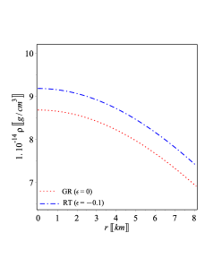
(a)  The energy-density

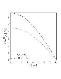
(b)  The radial pressure

(c)  The tangential pressure

Figure 1: Plots of the density, radial and tangential pressures given by (3) versus the radial coordinate $r$ in km of the pulsar Her X-1 ($M=0.85\pm 0.15M_{\odot}$, $R=8.1\pm 0.41$ km). We set $\epsilon=-0.1$, $a_{0}\approx 0.369$, $a_{1}\approx-0.622$ and $a_{2}\approx 0.298$.

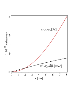
(a)  Anisotropy and anisotropic force

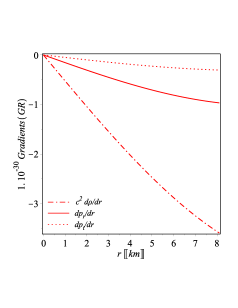
(b)  Gradients ($\epsilon=0$)

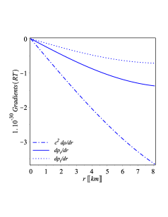
(c)  Gradients ($\epsilon=-0.14$)

Figure 2: Plot of the anisotropy parameter (19), anisotropic force $F_{a}=2\Delta/r$. We note that the Rastall parameter has no contribution in the anisotropy, therefore GR and RT predicts same anisotropy in the case of spherical symmetry as discussed after (16). For $\epsilon=0$ and $\epsilon\neq 0$, the gradients of the density, tangential and radial pressures given by Eqs. (29)–(31) versus the radial coordinate $r$ in km of the pulsar Her X-1.

Next, we use the above expressions to plot some physical quantities for $\epsilon=0$ (GR case) and $\epsilon\neq 0$ (RT case) which enable us to test the model viability and investigate the role of Rastall parameter. We note that one should be careful for the choice of Rastall parameter in order to satisfy the physical conditions in Sec. 4 with a particular compact object. In agreement with Oliveira et al. Oliveira:2015lka we confirm that the present model is physically stable whereas the Rastall parameter $\epsilon$ is negative. For the particular pulsar Her X-1, setting $\epsilon=-0.1$, we determine the set of constants $a_{0}\approx 0.369$, $a_{1}\approx-0.622$ and $a_{2}\approx 0.298$, which clearly satisfies Zeldovich condition (28).

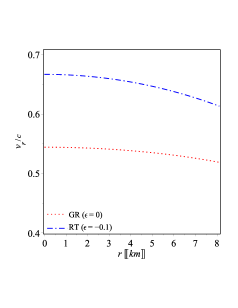
(a)  Radial speed of sound

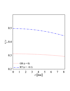
(b)  Tangential speed of sound

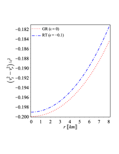
(c)  difference between radial and tangential speed of sounds

Figure 3: The radial and tangential sound speeds (30) versus the radial coordinate $r$ in km for the pulsar Her X-1. The plots confirm that the model fulfill the causality and the stability conditions (viii) and (ix) in Sec. 4.

(a)  Weak energy conditions

(b)  Null energy conditions

(c)  Strong energy condition

(d)  Dominant energy condition (radial)

(e)  Dominant energy condition (tangential)

Figure 4: The weak, null, strong and dominant energy conditions, using Eqs. (3), versus the radial coordinate $r$ in km for the pulsar Her X-1. The plots show that the model fulfill the energy conditions (vii) in Sec. 4.

In Figs. 10(a)–0(c), recalling condition (iii) in Sec. 4, we represent the behavior of energy-density, radial and tangential pressures for the pulsar Her X-1 from its center to the boundary surface. This shows that the density, radial and tangential pressures are positive as required for realistic stellar configuration with maximal finite values at the center decrease monotonically towards the surface. Also, as Fig. 1 0(a) shows, the surface density is above $7\times 10^{14}$ g/cm³ while the central density is comparable to the nuclear density $\sim 10^{15}$ g/cm³ which indicate that the pulsar Her X-1 may has no neutron core but quark-gluon one. This will be revisited in Sec. 8. In addition, Fig. 10(b) shows that the radial pressure at the surface is null in agreement with condition (v) in Sec. 4.

In Fig. 21(a), recalling condition (iv) in Sec. 4, we show that the anisotropy parameter (19) is null at the center and increases monotonically toward the surface of the star. Also, it shows that the anisotropic force $F_{a}=\frac{2\Delta}{r}$ is positive reflecting the repulsive behaviour of the force as $p_{t}-p_{r}>0$. Recalling Eq. (16) we verify that the Rastall parameter has no contribution to the anisotropy parameter so both GR ($\epsilon=0$) and RT ($\epsilon\neq 0$) cases coincide. However, this is not the case with other ingredients. For the GR ($\epsilon=0$) and RT ($\epsilon\neq 0$) cases, Figs. 2 1(b) and 1(c) respectively confirm that the gradients of energy-density, radial and tangential pressures, given by Eqs. (29)–(31), are negative everywhere inside the star as required by condition (iii) in Sec. 4.

Recalling the causality and stability conditions (viii) and (ix) in Sec. 4, in Fig. 3, for GR ($\epsilon=0$) and RT ($\epsilon\neq 0$) cases, we plot the radial and tangential sound speeds (30) where both have positive values less than one. This result confirms that the obtained stellar model is fulfilling the causality condition. In addition, we investigated the energy conditions as visualized in Fig. 4. The plots of Figs. 43(a)–3(d), for $\epsilon\neq 0$, prove that the model satisfies the WEC, NEC, SEC and DEC since the graphs are always obtained in positive energy regions. This confirms the fulfillment of the energy conditions (vii) in Sec. 4.

In Figs. 54(a) and 4(c), for $\epsilon=0$ and $\epsilon\neq 0$ cases, we plot the evolution of the radial and the tangential EoS parameters, i.e. $w_{r}(r)=p_{r}/\rho$ and $w_{t}(r)=p_{t}/\rho$, respectively, verses the radial distance from the center. The plots show that the EoS parameters slightly vary from maximum at the center with a monotonically decreasing behavior toward the surface whereas $w_{r}$ drops to zero at the surface as expected. We note that the variation of the EoS parameters is more severe in RT than GR, which should be understood as an effect of the matter-geometry coupling. On the other hand, we remind that there are no EoS are preassumed in the model setup, Figs. 54(b) and 4(d), however, prove that the EoS $p(\rho)$ in both radial and tangential directions is in well fit with linear patterns, whereas the best fit are given by $p_{r}=0.414\,\rho-27.6$ and $p_{t}=0.223\,\rho-11.8$ for the pulsar Her X-1. Notably the slopes of the fitted lines $dp_{r}/d\rho=0.414=v_{r}^{2}$ and $dp_{t}/d\rho=0.223=v_{t}^{2}$ are consistent with the corresponding values of Table 2 for the pulsar under investigation.

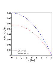
(a)  radial EoS parameter

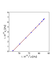
(b)  linear radial EoS

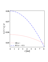
(c)  tangential EoS parameter

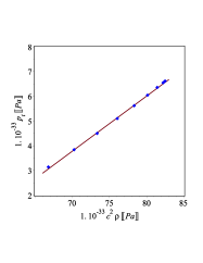
(d)  linear tangential EoS

Figure 5: Figs. 4(a) and 4(a) show the behaviours of the EoS parameters, defined as $w_{r}(r)=p_{r}/\rho$ and $w_{t}(r)=p_{t}/\rho$, at different radial distances within the pulsar Her X-1 as predicted by RT and GR. We note that no EoS are imposed at any stage of the present work, while it is evidently that the result fit well with the linear behaviour whereas the best fit lines in Fig. 4(b) and 4(d) are given by $p_{r}=0.414\,\rho-27.6$ and $p_{t}=0.223\,\rho-11.8$ in RT case.

The mass function given by Eq. (22) is plotted in Fig. 6 5(a) which shows that it is a monotonically increasing function of the radial coordinate whereas the mass at the center $M(r=0)=0$. The plot shows that theoretical $M(r)$ curve of the pulsar Her X-1 according to RT is compatible with the observed values of the mass and the radius. In Fig. 6 5(b) we show the behavior of the compactness parameter of the pulsar. Interestingly the RT curve allows less size than the GR for same mass which may evidently reflects the role of the matter-geometry coupling to obtain slightly higher compactness. Also Fig. 6 5(c) shows the redshift of the pulsar is maximum at the center and decreases monotonically toward the surface. Notably the redshift at the surface is found to be $Z_{R}\sim 0.204$ which is in an agreement with the upper bound constraints $Z_{R}\leq 2$ as given by Buchdahl PhysRev.116.1027 , for anisotropic spheres see Ivanov:2002xf ; PhysRevD.67.064003 and for the upper bound on the surface redshift in presence of a cosmological constant see Bohmer2006 .

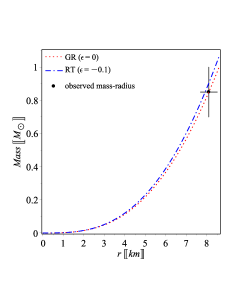
(a)  Mass function

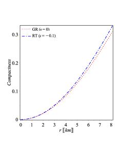
(b)  Compactness function

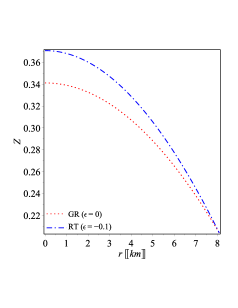
(c)  Red-shift function

Figure 6: The mass function plot confirm that the model can predict the a of the pulsar Her X-1 in agreement with observational data. The plot shows that RT predicts compactness values higher than GR which reflects the role of the matter-geometry coupling to allow more compactness values. The redshift is finite everywhere within the pulsar and decreases toward the surface as stated by condition (x) in Sec. 4 and also predict a surface redshift consistent with the upper limit constraints as given by Bohmer2006 .

7 Stability of the model

In addition to the stability condition (ix) in Sec. 4 which has been shown to be verified we are going to discuss the stability of the obtained stellar model using two different techniques in the present section; that are the modified TOV equations and the adiabatic index.

7.1 Equilibrium analysis via Tolman-Oppenheimer-Volkoff equation

We assume hydrostatic equilibrium to be everywhere within the stable compact star. This configuration, then, can be described by the GR based TOV equation PhysRev.55.364 ; PhysRev.55.374 ; PoncedeLeon1993 which gives the following stability constraint

$$\frac{2(p_{t}-p_{r})}{r}-\frac{M_{g}(\rho+p_{r})\sqrt{F}}{r\sqrt{G}}-\frac{dp_{r}}{dr}=0,$$ (37)

where $M=M_{g}(r)$ is the gravitational mass within a radius $r$, which is defined by the Tolman-Whittaker mass formula

$$M_{g}(r)=4\pi{\int_{0}}^{r}\Big{(}{T_{t}}^{t}-{T_{r}}^{r}-{T_{\theta}}^{\theta}-{T_{\phi}}^{\phi}\Big{)}r^{2}\sqrt{FG}dr=\frac{rF^{\prime}\sqrt{G}}{2F\sqrt{F}}\,.$$ (38)

Inserting Eq. (38) into (37), we get

$$\frac{2}{r}(p_{t}-p_{r})-\frac{F^{\prime}}{2F}(\rho+p_{r})-\frac{dp_{r}}{dr}=F_{a}+F_{g}+F_{h}=0\,,$$ (39)

where $F_{g}=-\frac{F^{\prime}}{2{F}}(\rho+p_{r})$ and $F_{h}=-\frac{dp_{r}}{dr}$ are the gravitational and the hydrostatic forces respectively, in addition to the anisotropic force $F_{a}$. We note that the TOV equation should be modified in RT due to the non-minimal coupling constraint, $\mathcal{T}{{}^{\alpha}}{{}_{\beta;\alpha}}=\epsilon\,\partial_{\beta}\mathcal{R}$, to include one more force $F_{R}$ as following

$$F_{a}+F_{g}+F_{h}+F_{R}=0\,,$$ (40)

where $F_{R}=-\frac{\epsilon}{1-4\epsilon}\frac{d}{dr}(\rho-p_{r}-2p_{t})$. These different forces, for GR ($\epsilon=0$) and RT ($\epsilon\neq 0$), are plotted in Fig. 7 using the pulsar Her X-1 data. For the RT case, the figure clearly shows that the pulsar is dominated by the negative gravitational force over the positive hydrostatics and anisotropic forces. Therefore, it holds the pulsar in a static equilibrium. In conclusion, we verify the stability of the model via TOV equation using the pulsar Her X-1 data.

(a)  TOV equation ($\epsilon=0$)

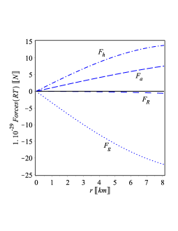
(b)  TOV equation ($\epsilon=-0.1$)

Figure 7: Plots of the forces of TOV equation (39) in cases $\epsilon=0$ and $\epsilon=-0.1$ versus the radius $r$ using the constants constrained from Her X-1. In the RT case the negative gravitational force is the dominant one over the hydrostatic and the anisotropic forces. This guarantees stable equilibrium configuration for the pulsar.

7.2 Relativistic adiabatic indices

Another verification of the stable equilibrium configuration of a spherically symmetric object can be done via the adiabatic index, that is defined as the ratio of two specific heats and can be given as follows 1964ApJ…140..417C ; 1989A&A…221….4M ; 10.1093/mnras/265.3.533

$$\Gamma=\frac{\rho+p_{r}}{p_{r}}v_{r}^{2}\,.$$ (41)

For the general case of anisotropic spheroid fluid, it has been shown that the object is in a neutral equilibrium if its adiabatic index $\Gamma=\gamma$ and in a stable equilibrium if $\Gamma>\gamma$ 10.1093/mnras/265.3.533 , whereas

$$\gamma=\frac{4}{3}\left(1+\frac{F_{a}}{2|p^{\prime}_{r}|}\right)_{max}\,.$$ (42)

Clearly, for an isotropic fluid, the object is in a neutral equilibrium if the adiabatic index $\Gamma=\frac{4}{3}$, while for $\Gamma>\frac{4}{3}$ the object is in a stable equilibrium 1975A&A….38…51H . Using Eq. (42), we get

$$\gamma = \frac{2}{3R^{8}}\biggl{[}\biggl{(}2R^{8}\biggl{|}\frac{r{a_{2}}^{4}}{{R}^{8}\left(a_{0}{R}^{2}+2a_{1}{a_{2}}^{2}{R}^{2}-2a_{1}{a_{2}}^{4}{r}^{2}\right)^{2}}\biggl{\{}216{r}^{8}{a_{1}}^{2}{a_{2}}^{12}\epsilon-12{r}^{8}{a_{1}}^{2}{a_{2}}^{12}+56{r}^{6}{R}^{2}{a_{1}}^{2}{a_{2}}^{10}-880{r}^{6}{R}^{2}{a_{1}}^{2}{a_{2}}^{10}\epsilon$$ (43)

$$+1352{r}^{4}{R}^{4}{a_{1}}^{2}{a_{2}}^{8}\epsilon-100{r}^{4}{R}^{4}{a_{1}}^{2}{a_{2}}^{8}-168{r}^{6}{R}^{2}a_{1}\,{a_{2}}^{8}a_{0}\epsilon-4\,{r}^{6}{R}^{2}a_{1}\,{a_{2}}^{8}a_{0}+80{r}^{2}{R}^{6}{a_{1}}^{2}{a_{2}}^{6}-928\,{r}^{2}{R}^{6}{a_{1}}^{2}{a_{2}}^{6}\epsilon+520{r}^{4}{R}^{4}a_{1}{a_{2}}^{6}a_{0}\epsilon$$

$$+4\,{r}^{4}{R}^{4}a_{1}\,{a_{2}}^{6}a_{0}+240\,{R}^{8}{a_{2}}^{4}{a_{1}}^{2}\epsilon-24\,{R}^{8}{a_{2}}^{4}{a_{1}}^{2}-544\,{R}^{6}{a_{2}}^{4}{r}^{2}a_{0}\,a_{1}\,\epsilon+8\,{R}^{6}{a_{2}}^{4}{r}^{2}a_{0}\,a_{1}+9\,{R}^{4}{a_{2}}^{4}{r}^{4}{a_{0}}^{2}+18\,{R}^{4}{a_{2}}^{4}{r}^{4}{a_{0}}^{2}\epsilon$$

$$-8\,a_{0}\,{R}^{8}{a_{2}}^{2}a_{1}+192\,a_{0}\,{R}^{8}{a_{2}}^{2}a_{1}\,\epsilon-16\,{a_{0}}^{2}{R}^{6}{a_{2}}^{2}{r}^{2}+24{a_{0}}^{2}{R}^{8}\epsilon-40{a_{0}}^{2}{R}^{6}{a_{2}}^{2}{r}^{2}\epsilon+6{a_{0}}^{2}{R}^{8}\biggr{\}}\biggr{|}+6{R}^{4}r{a_{2}}^{4}-8{R}^{2}{r}^{3}{a_{2}}^{6}+3{a_{2}}^{8}{r}^{5}\biggr{)}\biggl{|}$$

$$\biggl{\{}{R}^{8}\biggl{[}a_{0}{R}^{2}+2a_{1}\,{a_{2}}^{2}{R}^{2}-2a_{1}\,{a_{2}}^{4}{r}^{2}\biggr{]}^{2}\biggr{\}}\biggl{\{}r{a_{2}}^{4}\biggl{(}216\,{r}^{8}{a_{1}}^{2}{a_{2}}^{12}\epsilon-12\,{r}^{8}{a_{1}}^{2}{a_{2}}^{12}+56\,{r}^{6}{R}^{2}{a_{1}}^{2}{a_{2}}^{10}-880\,{r}^{6}{R}^{2}{a_{1}}^{2}{a_{2}}^{10}\epsilon$$

$$+1352{r}^{4}{R}^{4}{a_{1}}^{2}{a_{2}}^{8}\epsilon-100{r}^{4}{R}^{4}{a_{1}}^{2}{a_{2}}^{8}-168{r}^{6}{R}^{2}a_{1}{a_{2}}^{8}a_{0}\epsilon-4\,{r}^{6}{R}^{2}a_{1}{a_{2}}^{8}a_{0}+80\,{r}^{2}{R}^{6}{a_{1}}^{2}{a_{2}}^{6}-928{r}^{2}{R}^{6}{a_{1}}^{2}{a_{2}}^{6}\epsilon+520{r}^{4}{R}^{4}a_{1}{a_{2}}^{6}a_{0}\epsilon$$

$$+4\,{r}^{4}{R}^{4}a_{1}\,{a_{2}}^{6}a_{0}+240{R}^{8}{a_{2}}^{4}{a_{1}}^{2}\epsilon-24{R}^{8}{a_{2}}^{4}{a_{1}}^{2}-544{R}^{6}{a_{2}}^{4}{r}^{2}a_{0}a_{1}\,\epsilon+8{R}^{6}{a_{2}}^{4}{r}^{2}a_{0}a_{1}+9{R}^{4}{a_{2}}^{4}{r}^{4}{a_{0}}^{2}+18{R}^{4}{a_{2}}^{4}{r}^{4}{a_{0}}^{2}\epsilon$$

$$-8a_{0}\,{R}^{8}{a_{2}}^{2}a_{1}+192\,a_{0}\,{R}^{8}{a_{2}}^{2}a_{1}\,\epsilon-16\,{a_{0}}^{2}{R}^{6}{a_{2}}^{2}{r}^{2}-40\,{a_{0}}^{2}{R}^{6}{a_{2}}^{2}{r}^{2}\epsilon+6\,{a_{0}}^{2}{R}^{8}+24\,{a_{0}}^{2}{R}^{8}\epsilon\biggr{)}\biggr{\}}^{-1}\biggr{|}\biggr{]}\,.$$

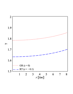
(a)  $\gamma$ in cases $\epsilon=0$ and $\epsilon\neq 0$

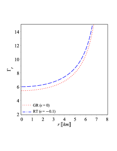
(b)  $\Gamma_{r}$ in cases $\epsilon=0$ and $\epsilon\neq 0$

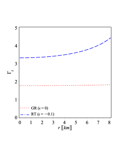
(c)  $\Gamma_{t}$ in cases $\epsilon=0$ and $\epsilon\neq 0$

Figure 8: Plots of the Adiabatic indices $\gamma$, $\Gamma_{r}$ and $\Gamma_{t}$, namely (43)–(45), versus the radius $r$ using the constants constrained from Her X-1. For RT, the adiabatic index $\gamma$ less than the GR case but still greater than the neutral equilibrium value $\gamma=\frac{4}{3}$. The radial and tangential adiabatic indices have higher values whereas the stability constraints $\Gamma_{r}>\gamma$ and $\Gamma_{t}>\gamma$ are fulfilled everywhere within the pulsar.

From Eq. (41), we obtain the adiabatic index of solution (3) in the form

$$\Gamma_{r} = -4\biggl{\{}\left(4a_{1}{a_{2}}^{2}{R}^{2}+3a_{0}{R}^{2}-4a_{1}{a_{2}}^{4}{r}^{2}\right)\left(R{}^{2}-a_{2}{}^{2}r^{2}\right)^{3}\biggl{[}216{r}^{8}{a_{1}}^{2}{a_{2}}^{12}\epsilon-12{r}^{8}{a_{1}}^{2}{a_{2}}^{12}+56{r}^{6}{R}^{2}{a_{1}}^{2}{a_{2}}^{10}-880{r}^{6}{R}^{2}{a_{1}}^{2}{a_{2}}^{10}\epsilon$$ (44)

$$+1352\,{r}^{4}{R}^{4}{a_{1}}^{2}{a_{2}}^{8}\epsilon-100\,{r}^{4}{R}^{4}{a_{1}}^{2}{a_{2}}^{8}-168\,{r}^{6}{R}^{2}a_{1}\,{a_{2}}^{8}a_{0}\,\epsilon-4\,{r}^{6}{R}^{2}a_{1}\,{a_{2}}^{8}a_{0}+80\,{r}^{2}{R}^{6}{a_{1}}^{2}{a_{2}}^{6}-928\,{r}^{2}{R}^{6}{a_{1}}^{2}{a_{2}}^{6}\epsilon$$

$$+520\,{r}^{4}{R}^{4}a_{1}\,{a_{2}}^{6}a_{0}\,\epsilon+4\,{r}^{4}{R}^{4}a_{1}\,{a_{2}}^{6}a_{0}+240\,{R}^{8}{a_{2}}^{4}{a_{1}}^{2}\epsilon-24\,{R}^{8}{a_{2}}^{4}{a_{1}}^{2}-544\,{R}^{6}{a_{2}}^{4}{r}^{2}a_{0}\,a_{1}\,\epsilon+8\,{R}^{6}{a_{2}}^{4}{r}^{2}a_{0}\,a_{1}$$

$$+9\,{R}^{4}{a_{2}}^{4}{r}^{4}{a_{0}}^{2}+18\,{R}^{4}{a_{2}}^{4}{r}^{4}{a_{0}}^{2}\epsilon-8\,a_{0}\,{R}^{8}{a_{2}}^{2}a_{1}+192\,a_{0}\,{R}^{8}{a_{2}}^{2}a_{1}\,\epsilon-16\,{a_{0}}^{2}{R}^{6}{a_{2}}^{2}{r}^{2}-40\,{a_{0}}^{2}{R}^{6}{a_{2}}^{2}{r}^{2}\epsilon+6\,{a_{0}}^{2}{R}^{8}$$

$$+24\,{a_{0}}^{2}{R}^{8}\epsilon\biggr{]}\biggr{\}}\biggl{\{}\biggl{[}36\,a_{1}\,{r}^{8}{a_{2}}^{10}\epsilon-2\,a_{1}\,{r}^{8}{a_{2}}^{10}+10\,{r}^{6}{R}^{2}a_{1}\,{a_{2}}^{8}-148\,{r}^{6}{R}^{2}a_{1}\,{a_{2}}^{8}\epsilon-20\,{r}^{4}{R}^{4}a_{1}\,{a_{2}}^{6}+232\,{R}^{4}{r}^{4}{a_{2}}^{6}a_{1}\,\epsilon$$

$$-3\,{R}^{2}{r}^{6}{a_{2}}^{6}a_{0}-6\,{R}^{2}{r}^{6}{a_{2}}^{6}a_{0}\,\epsilon+20\,{R}^{6}{r}^{2}{a_{2}}^{4}a_{1}-168\,{R}^{6}{r}^{2}{a_{2}}^{4}a_{1}\,\epsilon+8\,{R}^{4}{r}^{4}{a_{2}}^{4}a_{0}+20\,{R}^{4}{r}^{4}{a_{2}}^{4}a_{0}\,\epsilon-8\,{R}^{8}{a_{2}}^{2}a_{1}$$

$$+48\,{R}^{8}{a_{2}}^{2}a_{1}\,\epsilon-6\,{R}^{6}{a_{2}}^{2}{r}^{2}a_{0}-24\,{R}^{6}{a_{2}}^{2}{r}^{2}a_{0}\,\epsilon+12\,\epsilon\,{R}^{8}a_{0}\biggr{]}\biggl{[}216\,{r}^{8}{a_{1}}^{2}{a_{2}}^{12}\epsilon-108\,{r}^{8}{a_{1}}^{2}{a_{2}}^{12}+440\,{r}^{6}{R}^{2}{a_{1}}^{2}{a_{2}}^{10}$$

$$-880{r}^{6}{R}^{2}{a_{1}}^{2}{a_{2}}^{10}\epsilon-676{r}^{4}{R}^{4}{a_{1}}^{2}{a_{2}}^{8}+1352{r}^{4}{R}^{4}{a_{1}}^{2}{a_{2}}^{8}\epsilon-168{r}^{6}{R}^{2}a_{1}{a_{2}}^{8}a_{0}\epsilon+108\,{r}^{6}{R}^{2}a_{1}{a_{2}}^{8}a_{0}+464\,{r}^{2}{R}^{6}{a_{1}}^{2}{a_{2}}^{6}$$

$$-928\,{r}^{2}{R}^{6}{a_{1}}^{2}{a_{2}}^{6}\epsilon+520\,{r}^{4}{R}^{4}a_{1}\,{a_{2}}^{6}a_{0}\,\epsilon-332\,{r}^{4}{R}^{4}a_{1}\,{a_{2}}^{6}a_{0}-120\,{R}^{8}{a_{2}}^{4}{a_{1}}^{2}+240\,{R}^{8}{a_{2}}^{4}{a_{1}}^{2}\epsilon-544\,{R}^{6}{a_{2}}^{4}{r}^{2}a_{0}\,a_{1}\,\epsilon$$

$$+344\,{R}^{6}{a_{2}}^{4}{r}^{2}a_{0}\,a_{1}-27\,{R}^{4}{a_{2}}^{4}{r}^{4}{a_{0}}^{2}+18\,{R}^{4}{a_{2}}^{4}{r}^{4}{a_{0}}^{2}\epsilon-120\,a_{0}\,{R}^{8}{a_{2}}^{2}a_{1}+192\,a_{0}\,{R}^{8}{a_{2}}^{2}a_{1}\,\epsilon+56\,{a_{0}}^{2}{R}^{6}{a_{2}}^{2}{r}^{2}$$

$$-40\,{a_{0}}^{2}{R}^{6}{a_{2}}^{2}{r}^{2}\epsilon-30\,{a_{0}}^{2}{R}^{8}+24\,{a_{0}}^{2}{R}^{8}\epsilon\biggr{]}\biggr{\}}^{-1}\,,$$

and

$$\Gamma_{t} = -\biggl{\{}\biggl{[}108\,{r}^{8}{a_{1}}^{2}{a_{2}}^{12}\epsilon-24\,{r}^{8}{a_{1}}^{2}{a_{2}}^{12}+96\,{r}^{6}{R}^{2}{a_{1}}^{2}{a_{2}}^{10}-440\,{r}^{6}{R}^{2}{a_{1}}^{2}{a_{2}}^{10}\epsilon+676\,{r}^{4}{R}^{4}{a_{1}}^{2}{a_{2}}^{8}\epsilon-144\,{r}^{4}{R}^{4}{a_{1}}^{2}{a_{2}}^{8}$$ (45)

$$-84\,{r}^{6}{R}^{2}a_{1}\,{a_{2}}^{8}a_{0}\,\epsilon+16\,{r}^{6}{R}^{2}a_{1}\,{a_{2}}^{8}a_{0}-464\,{r}^{2}{R}^{6}{a_{1}}^{2}{a_{2}}^{6}\epsilon+96\,{r}^{2}{R}^{6}{a_{1}}^{2}{a_{2}}^{6}+260\,{r}^{4}{R}^{4}a_{1}\,{a_{2}}^{6}a_{0}\,\epsilon-48\,{r}^{4}{R}^{4}a_{1}\,{a_{2}}^{6}a_{0}$$

$$-24{R}^{8}{a_{2}}^{4}{a_{1}}^{2}+120{R}^{8}{a_{2}}^{4}{a_{1}}^{2}\epsilon-272{R}^{6}{a_{2}}^{4}{r}^{2}a_{0}a_{1}\,\epsilon+48{R}^{6}{a_{2}}^{4}{r}^{2}a_{0}a_{1}+9\,{R}^{4}{a_{2}}^{4}{r}^{4}{a_{0}}^{2}\epsilon-16a_{0}\,{R}^{8}{a_{2}}^{2}a_{1}+12\,{a_{0}}^{2}{R}^{8}\epsilon$$

$$+96\,a_{0}\,{R}^{8}{a_{2}}^{2}a_{1}\,\epsilon-20\,{a_{0}}^{2}{R}^{6}{a_{2}}^{2}{r}^{2}\epsilon\biggr{]}\biggl{[}10\,a_{1}\,{r}^{8}{a_{2}}^{10}-42\,{r}^{6}{R}^{2}a_{1}\,{a_{2}}^{8}-9\,{R}^{2}{r}^{6}{a_{2}}^{6}a_{0}+68\,{r}^{4}{R}^{4}a_{1}\,{a_{2}}^{6}+28\,{R}^{4}{r}^{4}{a_{2}}^{4}a_{0}$$

$$-52{R}^{6}{r}^{2}{a_{2}}^{4}a_{1}-30{R}^{6}{a_{2}}^{2}{r}^{2}a_{0}+16{R}^{8}{a_{2}}^{2}a_{1}+12a_{0}\,{R}^{8}\biggr{]}\biggr{\}}\biggl{\{}\biggl{[}18a_{1}{r}^{8}{a_{2}}^{10}\epsilon-4a_{1}\,{r}^{8}{a_{2}}^{10}-74{r}^{6}{R}^{2}a_{1}{a_{2}}^{8}\epsilon+16\,{r}^{6}{R}^{2}a_{1}\,{a_{2}}^{8}$$

$$+116\,{R}^{4}{r}^{4}{a_{2}}^{6}a_{1}\,\epsilon-24\,{r}^{4}{R}^{4}a_{1}\,{a_{2}}^{6}-3\,{R}^{2}{r}^{6}{a_{2}}^{6}a_{0}\,\epsilon-84\,{R}^{6}{r}^{2}{a_{2}}^{4}a_{1}\,\epsilon+16\,{R}^{6}{r}^{2}{a_{2}}^{4}a_{1}+10\,{R}^{4}{r}^{4}{a_{2}}^{4}a_{0}\,\epsilon-4\,{R}^{8}{a_{2}}^{2}a_{1}$$

$$+24\,{R}^{8}{a_{2}}^{2}a_{1}\,\epsilon-12\,{R}^{6}{a_{2}}^{2}{r}^{2}a_{0}\,\epsilon+6\,\epsilon\,{R}^{8}a_{0}\biggr{]}\biggl{[}216\,{r}^{8}{a_{1}}^{2}{a_{2}}^{12}\epsilon-108\,{r}^{8}{a_{1}}^{2}{a_{2}}^{12}+440\,{r}^{6}{R}^{2}{a_{1}}^{2}{a_{2}}^{10}-880\,{r}^{6}{R}^{2}{a_{1}}^{2}{a_{2}}^{10}\epsilon$$

$$-676\,{r}^{4}{R}^{4}{a_{1}}^{2}{a_{2}}^{8}+1352\,{r}^{4}{R}^{4}{a_{1}}^{2}{a_{2}}^{8}\epsilon-168\,{r}^{6}{R}^{2}a_{1}\,{a_{2}}^{8}a_{0}\,\epsilon+108\,{r}^{6}{R}^{2}a_{1}\,{a_{2}}^{8}a_{0}+464\,{r}^{2}{R}^{6}{a_{1}}^{2}{a_{2}}^{6}-928\,{r}^{2}{R}^{6}{a_{1}}^{2}{a_{2}}^{6}\epsilon$$

$$+520\,{r}^{4}{R}^{4}a_{1}\,{a_{2}}^{6}a_{0}\,\epsilon-332\,{r}^{4}{R}^{4}a_{1}\,{a_{2}}^{6}a_{0}-120\,{R}^{8}{a_{2}}^{4}{a_{1}}^{2}+240\,{R}^{8}{a_{2}}^{4}{a_{1}}^{2}\epsilon-544\,{R}^{6}{a_{2}}^{4}{r}^{2}a_{0}\,a_{1}\,\epsilon+344\,{R}^{6}{a_{2}}^{4}{r}^{2}a_{0}\,a_{1}$$

$$-27\,{R}^{4}{a_{2}}^{4}{r}^{4}{a_{0}}^{2}+18\,{R}^{4}{a_{2}}^{4}{r}^{4}{a_{0}}^{2}\epsilon-120\,a_{0}\,{R}^{8}{a_{2}}^{2}a_{1}+192\,a_{0}\,{R}^{8}{a_{2}}^{2}a_{1}\,\epsilon+56\,{a_{0}}^{2}{R}^{6}{a_{2}}^{2}{r}^{2}-40\,{a_{0}}^{2}{R}^{6}{a_{2}}^{2}{r}^{2}\epsilon$$

$$-30\,{a_{0}}^{2}{R}^{8}+24\,{a_{0}}^{2}{R}^{8}\epsilon\biggr{]}\biggr{\}}\,.$$

In Figs. 87(a)–7(c), we plot the profiles of the adiabatic indices $\gamma$, $\Gamma_{r}$ and $\Gamma_{t}$ of the pulsar Her X-1, respectively. It is clear that the value of the adiabatic index $\gamma$ as predicted by RT is less than the corresponding GR value everywhere within the pulsar. On the other hand, the other adiabatic indices $\Gamma_{r}$ and $\Gamma_{t}$ are higher in RT than GR, whereas the stability constraints, namely $\Gamma_{r}>\gamma$ and $\Gamma_{t}>\gamma$, as shown in the figures are clearly fulfilled.

8 More Observational Constraints

In this section we confront the present model with other pulsars’ data to examine its validity with wide range of astrophysical observations. Also, we plot the mass-radius profile corresponding to different choices of the surface density compatible with the nuclear saturation density as boundary conditions showing the capability of the model to predict masses in the lower mass gap $2.5-5M_{\odot}$. On the other hand, we confront the compactness parameter as predicted by the model with Buchdahl compactness bound.

8.1 Pulsars’ data

In addition to Her X-1, a similar analysis is developed for other twenty one pulsars cover a wide range of masses from $0.8M_{\odot}$ to heavy pulsars of mass $2.01M_{\odot}$. In Table 1, we give the observed masses and radii for each associated with the corresponding model parameters {$a_{0}$, $a_{1}$, $a_{2}$} assuming that the Rastall parameter $\epsilon=-0.1$. We confirm that the model at hand can predict masses of those pulsars compatible with their observed values. In Table 2, we give the calculated values of physical quantities of most interest. As seen the values of the density are consistent with the nuclear density. It is to be mentioned that there are no EoSs are assumed, the obtained results however fit well with the linear behaviour, whereas the slopes $dp_{r}/d\rho$ and $dp_{t}/d\rho$ of the best fit lines are consistent with the values as obtained in Table 2. On the other hand these values confirm that the model is stable and causal for each case and satisfies all the physical constraints in Sec. 4. We additionally give the surface redshift values as predicted by the present model for the listed pulsars. All values are clearly in agreement with the upper bound constraint $Z_{R}\leq 2$ as given by Buchdahl PhysRev.116.1027 , also for anisotropic spheres see Ivanov:2002xf ; PhysRevD.67.064003 .

Table 1: Observed mass-radius of twenty pulsars and the corresponding model parameters ($\epsilon=-0.1$).

Pulsar	Ref.	observed mass ($M_{\odot}$)	observed radius [km]	estimated mass ($M_{\odot}$)	$a_{0}$	$a_{1}$	$a_{2}$
Her X-1	Abubekerov_2008	$0.85\pm 0.15$	$8.1\pm 0.41$	$0.905$	$0.369$	$-0.622$	$0.298$
RX J185635-3754	2002ApJ…564..981P	$0.9\pm 0.2$	$6$	$0.949$	$0.517$	$-0.706$	$0.369$
LMC X-4	Rawls:2011jw	$1.04\pm 0.09$	$8.301\pm 0.2$	$1.103$	$0.375$	$-0.658$	$0.330$
GW170817-2	LIGOScientific:2018cki	$1.27\pm 0.09$	$11.9\pm 1.4$	$1.351$	$0.437$	$-0.625$	$0.301$
EXO 1785-248	Ozel:2008kb	$1.3\pm 0.2$	$8.849\pm 0.4$	$1.372$	$0.507$	$-0.699$	$0.364$
PSR J0740+6620	Raaijmakers:2019qny	$1.34\pm 0.16$	$12.71\pm 1.19$	$1.426$	$0.370$	$-0.623$	$0.298$
M13	Webb:2007tc	$1.38\pm 0.2$	$9.95\pm 0.27$	$1.459$	$0.481$	$-0.683$	$0.351$
LIGO	LIGOScientific:2020zkf	$1.4$	$12.9\pm 0.8$	$1.489$	$0.381$	$-0.628$	$0.303$
X7	Rybicki:2005id	$1.4$	$14.5\pm 1.8$	$1.492$	$0.340$	$-0.607$	$0.284$
PSR J0037-4715	Reardon:2015kba	$1.44\pm 0.07$	$13.6\pm 0.9$	$1.532$	$0.372$	$-0.623$	$0.299$
PSR J0740+6620	Miller:2019cac	$1.44\pm 0.16$	$13.02\pm 1.24$	$1.531$	$0.388$	$-0.632$	$0.307$
GW170817-1	LIGOScientific:2018cki	$1.45\pm 0.09$	$11.9\pm 1.4$	$1.539$	$0.425$	$-0.652$	$0.325$
4U 1820-30	G_ver_2010	$1.46\pm 0.2$	$11.1\pm 1.8$	$1.546$	$0.457$	$-0.670$	$0.440$
Cen X-3	Naik:2011qc	$1.49\pm 0.49$	$9.178\pm 0.13$	$1.566$	$0.556$	$-0.731$	$0.388$
4U 1608-52	1996IAUC.6331….1M	$1.57\pm 0.3$	$9.8\pm 1.8$	$1.651$	$0.550$	$-0.727$	$0.385$
KS 1731-260	Ozel:2008kb	$1.61\pm 0.37$	$10\pm 2.2$	$1.692$	$0.552$	$-0.728$	$0.386$
EXO 1745-268	Ozel:2008kb	$1.65\pm 0.25$	$10.5\pm 1.8$	$1.736$	$0.540$	$-0.720$	$0.380$
Vela X-1	Rawls:2011jw	$1.77\pm 0.08$	$9.56\pm 0.08$	$1.845$	$0.627$	$-0.781$	$0.424$
4U 1724-207	Ozel:2008kb	$1.81\pm 0.27$	$12.2\pm 1.4$	$1.909$	$0.512$	$-0.702$	$0.366$
SAX J1748.9-2021	Ozel:2008kb	$1.81\pm 0.3$	$11.7\pm 1.7$	$1.906$	$0.532$	$-0.715$	$0.376$
PSR J1614-2230	Demorest:2010bx	$1.97\pm 0.04$	$13\pm 2$	$2.076$	$0.522$	$-0.709$	$0.371$
PSR J0348+0432	Antoniadis:2013pzd	$2.01\pm 0.04$	$13\pm 2$	$2.117$	$0.532$	$-0.715$	$0.376$

Table 2: Calculated physical quantities of the most interest.

Pulsar	$\rho(0)$	$\rho_{R}$	$v_{r}^{2}(0)/c^{2}$	$v_{r}^{2}(R)/c^{2}$	$v_{t}^{2}(0)/c^{2}$	$v_{t}^{2}(R)/c^{2}$	$\rho c^{2}-p_{r}-2p_{t}|_{0}$	$\rho-p_{r}-2p_{t}|_{R}$	$Z_{R}$
	[$g/cm^{3}$]	[$g/cm^{3}$]					[$Pa$]	[$Pa$]
Her X-1	9.18$\times 10^{14}$	7.39$\times 10^{14}$	0.445	0.376	0.246	0.195	6.27$\times 10^{34}$	5.73$\times 10^{34}$	0.204
RX J185635-3754	2.53$\times 10^{15}$	1.81$\times 10^{15}$	0.608	0.451	0.402	0.276	1.25$\times 10^{35}$	1.26$\times 10^{35}$	0.340
LMC X-4	1.07$\times 10^{15}$	8.19$\times 10^{14}$	0.506	0.406	0.304	0.228	6.53$\times 10^{34}$	6.08$\times 10^{34}$	0.260
GW170817-2	4.33$\times 10^{14}$	3.48$\times 10^{14}$	0.450	0.379	0.250	0.198	2.93$\times 10^{34}$	2.68$\times 10^{34}$	0.208
EXO 1785-248	1.13$\times 10^{15}$	8.21$\times 10^{14}$	0.593	0.444	0.388	0.269	5.80$\times 10^{34}$	5.76$\times 10^{34}$	0.329
PSR J0740+6620	3.75$\times 10^{14}$	3.01$\times 10^{14}$	0.446	0.377	0.247	0.196	2.55$\times 10^{34}$	2.33$\times 10^{34}$	0.205
M13	8.39$\times 10^{14}$	6.20$\times 10^{14}$	0.556	0.429	0.353	0.253	4.63$\times 10^{34}$	4.45$\times 10^{34}$	0.302
LIGO	3.76$\times 10^{14}$	3.00$\times 10^{14}$	0.454	0.381	0.255	0.201	2.52$\times 10^{34}$	2.31$\times 10^{34}$	0.213
X7	2.61$\times 10^{14}$	2.14$\times 10^{14}$	0.424	0.366	0.226	0.183	1.85$\times 10^{34}$	1.69$\times 10^{34}$	0.183
PSR J0037-4715	3.29$\times 10^{14}$	2.64$\times 10^{14}$	0.447	0.378	0.248	0.197	2.24$\times 10^{34}$	2.04$\times 10^{34}$	0.206
PSR J0740+6620	3.77$\times 10^{14}$	2.99$\times 10^{14}$	0.460	0.384	0.260	0.204	2.50$\times 10^{34}$	2.29$\times 10^{34}$	0.219
GW170817-1	5.04$\times 10^{14}$	3.89$\times 10^{14}$	0.494	0.401	0.293	0.222	3.14$\times 10^{34}$	2.91$\times 10^{34}$	0.250
4U 1820-30	6.33$\times 10^{14}$	4.77$\times 10^{14}$	0.528	0.416	0.325	0.239	3.70$\times 10^{34}$	3.49$\times 10^{34}$	0.279
Cen X-3	1.19$\times 10^{15}$	8.24$\times 10^{14}$	0.677	0.477	0.469	0.305	4.98$\times 10^{34}$	5.51$\times 10^{34}$	0.386
4U 1608-52	1.03$\times 10^{15}$	7.15$\times 10^{14}$	0.664	0.472	0.456	0.300	4.45$\times 10^{34}$	4.82$\times 10^{34}$	0.378
KS 1731-260	9.92$\times 10^{14}$	6.89$\times 10^{14}$	0.669	0.474	0.461	0.302	4.24$\times 10^{34}$	4.63$\times 10^{34}$	0.381
EXO 1745-268	8.74$\times 10^{14}$	6.14$\times 10^{14}$	0.646	0.466	0.439	0.293	3.95$\times 10^{34}$	4.18$\times 10^{34}$	0.366
Vela X-1	1.29$\times 10^{15}$	8.33$\times 10^{14}$	0.861	0.538	0.645	0.371	3.01$\times 10^{34}$	5.11$\times 10^{34}$	0.486
4U 1724-207	6.04$\times 10^{14}$	4.35$\times 10^{14}$	0.600	0.447	0.394	0.273	3.04$\times 10^{34}$	3.04$\times 10^{34}$	0.334
SAX J1748.9-2021	6.91$\times 10^{14}$	4.89$\times 10^{14}$	0.633	0.460	0.426	0.287	3.22$\times 10^{34}$	3.35$\times 10^{34}$	0.357
PSR J1614-2230	5.46$\times 10^{14}$	3.90$\times 10^{14}$	0.616	0.454	0.410	0.280	2.65$\times 10^{34}$	2.70$\times 10^{34}$	0.346
PSR J0348+0432	5.59$\times 10^{14}$	3.96$\times 10^{14}$	0.632	0.460	0.425	0.287	2.61$\times 10^{34}$	2.71$\times 10^{34}$	0.357

8.2 Mass-Radius Profile

As is shown in Table 2 the surface densities of the listed pulsars, $2.14\times 10^{14}\lesssim\rho_{R}\lesssim 1.81\times 10^{15}$ g/cm³, are mostly compatible with a neutron core. For four different values of the surface density of the pulsars $\rho_{R}=2.7\times 10^{14}$ g/cm³, $4\times 10^{14}$ g/cm³, $6\times 10^{14}$ g/cm³ and $8\times 10^{14}$ g/cm³ we plot the corresponding compactness-radius curve as in Fig. 98(a). In all cases the maximum compactness values do not exceed unity. However for a compact object to be stable it should satisfy Buchdahl compactness bound $U=\frac{2G_{N}M}{c^{2}R}\leq 8/9$ (for isotropic sphere PhysRev.116.1027 ). We visualize Buchdahl upper bound on the compactness parameter with the corresponding maximum radii as obtained for the four surface densities. It is convenient to give the model parameters {$a_{0}$, $a_{1}$, $a_{2}$} in terms of the total compactness parameter $U$. Recalling the matching conditions (35) and (36) we write

$$a_{0} = \small{3\left\{\left[(U-\frac{8}{9})(1-U)^{\frac{1}{4}}+\frac{8}{9}(1-U)\right]\epsilon-\frac{1}{18}(1-U)^{\frac{1}{4}}U\right\}\sqrt{-(1-U)^{2}(U-2+4(1-U)^{\frac{3}{4}}-6\sqrt{1-U}+4(1-U)^{\frac{1}{4}})}\over\left[-\frac{1}{2}(1-U)^{\frac{1}{4}}+\sqrt{1-U}-\frac{1}{2}(1-U)^{\frac{3}{4}}\right](\epsilon-\frac{1}{3})(U-1)},$$

$$a_{1} = -\frac{1}{2}{\left(\sqrt{1-U}-(1-U)^{\frac{3}{4}}\right)a_{0}+4\sqrt{-(1-U)^{2}(U-2+4(1-U)^{\frac{3}{4}}-6\sqrt{1-U}+4(1-U)^{\frac{1}{4}})}\over U-\sqrt{1-U}+2(1-U)^{\frac{3}{4}}-1},$$

$$a_{2} = \sqrt{1-(1-U)^{1/4}}.$$ (46)

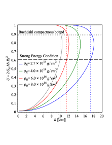
(a)  Compactness-Radius

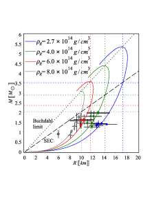
(b)  Mass-Radius

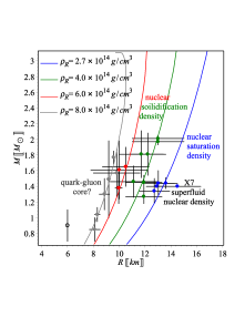
(c)  Neutron star core

Figure 9: 8(a) Compactness-radius profiles for four surface densities, the horizontal dot and dash lines visualize Buchdahl ($U=8/9$) and the SEC bound ($U(\epsilon=-0.1)=0.603$) on the compactness parameter. Clearly both constraints give almost the same maximum radii. 8(b) Mass-radius profiles for four surface densities combined with observed mass-radius values of the pulsars in Table 1. The diagonal dot and dash lines set Buchdahl and SEC physical regions. Clearly all pulsars are below the SEC exclusion limit. The horizontal dot lines give the maximum possible mass as obtained by the SEC. 8(c) Pulsars on the red, green and blue mass-radius profiles are suggested to have neutron cores whereas the surface densities match superfluid, saturated, solidified nuclear densities. The pulsars on the gray mass-radius profile match perfectly a surface density boundary condition $\rho_{R}=8\times 10^{14}$ g/cm³ which may suggest quark-gluon cores for those pulsars.

Notably for the pulsar Her X-1 with $\epsilon=-0.1$, the compactness parameter $U=0.31$, which reproduces the set of constants $a_{0}\approx 0.369$, $a_{1}\approx-0.622$ and $a_{2}\approx 0.298$ as previously obtained in Sec. 6. Using Buchdahl limit $U=8/9$, we obtain the maximum radii $R=17.66$ km for $\rho_{R}=2.7\times 10^{14}$ g/cm³, $R=14.51$ km for $\rho_{R}=4\times 10^{14}$ g/cm³, $R=11.85$ km for $\rho_{R}=6\times 10^{14}$ g/cm³ and $R=10.26$ km for $\rho_{R}=8\times 10^{14}$ g/cm³. However, more restricted values on the maximum compactness can be imposed by utilizing the SEC as obtained in the present model. Thus we write the density, radial and tangential pressures, namely (3), in terms of the compactness parameter $U$, after straight forward calculations we find that the SEC is satisfied when the compactness $U\leq 0.603$ (using $\epsilon=-0.1$). Higher $U$ values can be obtained for higher values of $\epsilon$, e.g. $U(\epsilon=-0.05)\lesssim 0.639$. However, we restrict our discussion to $\epsilon=-0.1$. We visualize the SEC constraint on the upper compactness value as in Fig. 98(a). It can be seen that the lower $U$ value as obtained by the SEC gives almost the same maximum radii as Buchdahl compactness bound or slightly lesser. However, it puts more restricted values on the maximum masses as will be discussed shortly. For a compact object to be physically stable we use $U\leq 0.603$ as obtained by the SEC. This determines the maximum radii as allowed by the present model as $R=17.30$ km for $\rho_{R}=2.7\times 10^{14}$ g/cm³, $R=14.22$ km for $\rho_{R}=4\times 10^{14}$ g/cm³, $R=11.61$ km for $\rho_{R}=6\times 10^{14}$ g/cm³ and $R=10.05$ km for $\rho_{R}=8\times 10^{14}$ g/cm³.

In Fig. 98(b), we plot the mass-radius relation as obtained by the present model for the four surface densities along with the scatter plot of the observed mass-radius of the pulsars listed in Table 1. Consequently, we determine the maximum masses allowed by the present model according to Buchdahl limit for the surface densities $\rho_{R}=2.7\times 10^{14}$ g/cm³, $4\times 10^{14}$ g/cm³, $6\times 10^{14}$ g/cm³ and $8\times 10^{14}$ g/cm³, which have been found to be $5.31M_{\odot}$, $4.37M_{\odot}$, $3.56M_{\odot}$ and $3.09M_{\odot}$ respectively. In comparison with the GR case as obtained by Das et al. Das:2019dkn , RT allows more masses. Indeed these values provide unstable models, since they do not satisfy the SEC. We use the maximum compactness as obtained by the SEC, $U=0.603$, which determines the physically stable pulsars with maximum masses $3.53M_{\odot}$, $2.90M_{\odot}$, $2.37M_{\odot}$ and $2.05M_{\odot}$. Obviously from Fig. 98(b) all pulsars are below the SEC exclusion limit.

In Fig. 98(c), we split the pulsars into four groups according their matching with the mass-radius profiles of the surface densities. Notably, the nuclear saturation density $\rho_{\text{sat}}=2.7\times 10^{14}$ g/cm³ and solidification density $\rho_{\text{solid}}$ is expected to be from $2.8\times 10^{14}$ g/cm³ to $5\times 10^{14}$ g/cm³ whereas the maximum density of cold matter $\rho_{\text{max}}\lesssim 4\times 10^{15}$ g/cm³ based on an EoS-independent analytic solutions of Einstein field equations. In the present work, we find that the pulsar X7 has a neutron core with density less than $\rho_{\text{sat}}$ which matches anisotropic superfluid nuclear density $\sim 1.5\times 10^{14}$ g/cm³. The pulsars PSR J0030+0451, PSR J0037-4715 and the LIGO constraints have a neutron core with density matches $\rho_{\text{sat}}$. The pulsars M13, KS 1731-260, EXO 1745-268, GW170817-2, GW170817-1, 4U 1820-30, 4U 1724-207 and SAX J1748.9-2021 have a neutron core with density $\sim\rho_{\text{solid}}$. Notably, the most heaviest pulsars PSR J1614-2230 and PSR J0348+0432 fit well with the mass-radius curve corresponding to surface density $4\times 10^{14}$ g/cm³ which suggests that these pulsars are having solidified neutron cores. Similarly, the pulsars Her X-1, LMC X-4, EXO 1785-248, Cen X-3, 4U 1608-52 and Vela X-1 lie beyond neutron core density and match perfectly with mass-radius curve with a surface density of $\rho_{R}=8\times 10^{14}$ g/cm³, this suggests that those pulsars may have quark-gluon cores. This claim should be verified by gravitational wave signals and by experimental tests. It is to be mentioned that the four categories presented here fit well with linear EoS as is shown earlier in Fig. 5 whereas their slopes are given in Table 2.

Interestingly, the obtained curves allow for a heavy neutron star to lie in the lower mass gap $2.5-5M_{\odot}$ which keeps an open window for the binary secondary companion GW190814 LIGOScientific:2020zkf to be a neutron star with an anisotropic core whereas the EoS $p_{r}(\rho)$ and $p_{t}(\rho)$ are obtained by simple linear relations. Clearly RT (with $\epsilon<0$), using Buchdahl limit, allows for higher maximum masses than the corresponding results as obtained by Das et al. within the GR framework Das:2019dkn . This result is consistent with our earlier conclusion after Fig. 65(a) and also in agreement with the previous study of isotropic neutron stars in RT by Oliveira et al. Oliveira:2015lka . However, in the present work we investigate anisotropic compact objects without assuming any EoS. In the following section we summarize and conclude the present work.

9 Summary and conclusions

One way to modify GR is to drop one of its main assumptions. Rastall questioned the local conservation in presence of curved spacetime, which led him to a set of field equations consistent with a different assumption, that is a non-minimal coupling between matter and geometry whereas the energy-momentum tensor $\mathcal{T}{{}^{\alpha}}{{}_{\beta;\alpha}}\propto\mathcal{R}_{;\beta}$. Vissar, recently, claimed that RT is completely equivalent to GR Visser:2017gpz . On the contrary, Darabi et al. investigated Visser’s claim but they concluded that Visser misinterpreted the matter-geometry coupling term, and consequently led him to a wrong conclusion Darabi:2017coc . In addition, they showed that by applying Visser’s approach to $f(R)$ theory one may conclude that it is equivalent to GR as well, which is not true. One of the good examples which may reveal the contribution of the matter-geometry coupling in RT in contrast to GR is the stellar models when the presence of matter play a crucial role. In this study, we applied RT to anisotropic static star with spherical symmetry seeking for a non-trivial interior solution. We showed that, for static spherically symmetric stellar model, the Rastall parameter in general does not contribute to the anisotropy parameter while it contributes non-trivially to the density and the radial/tangential pressures. Applying appropriate ansatz we derived the corresponding density and pressure forms.

We matched the interior solution to the exterior Schwarzschild one (which is a solution in RT as well) in the case of the pulsar Her X-1 ($M=0.85\pm 0.15\,M_{\odot},\,R=8.1\pm 0.41$ km) and by recalling Zeldovich constraint, we determine the numerical values of the set of constants {$a_{0}$, $a_{1}$ and $a_{2}$} for a particular choice of Rastall parameter which has been found as $\epsilon=-0.1$. We verified that the obtained model satisfies the physical constraints as listed in Sec. 4 and their predictions are slightly different from GR ones. We give detailed patterns of all physical quantities in Figs. 1–8. In addition, we confronted the model at hand with other pulsars’ observations and we confirm that all physical conditions are fulfilled in all cases. In Table 1, we give the numerical values of the set of constants for the same Rastall parameter value $\epsilon=-0.1$ of twenty additional pulsars as is done in the case of the pulsar Her X-1 . Also, in Table 2, we give the corresponding physical quantities of the most interest for all pulsar at the present study. All results confirm that the model satisfies the physical conditions as listed in Sec. 4.

For four surface densities, we utilized the SEC to set an upper limit of the compactness $U\sim 0.603$ (where $\epsilon=-0.1$) less than Buchdahl compactness $U=8/9$, see Fig. 9. Consequently we determine the maximum possible masses with a stable configuration. For a boundary density compatible with neutron star core at saturation nuclear density the maximum mass $\sim 3.53M_{\odot}$. This results have been obtained without assuming a specific EoS, however, the pressure-density relation fits well with linear behaviour whereas the slopes keep a stable and causal structures. We split the twenty pulsars into four groups, three groups fit well with neutron cores with anisotropic superfluid, saturated and solidified cores. We found that the most massive pulsars PSR J1614-2230 and PSR J0348+0432 fit will with the mass-radius curve corresponding to surface density $4\times 10^{14}$ g/cm³ which suggests that those pulsars are having solidified neutron cores. Furthermore, we suggest that the following group of pulsars to have a quark-gluon cores, Her X-1, LMC X-4, EXO 1785-248, Cen X-3, 4U 1608-52 and Vela X-1. This group fit perfectly with a boundary density $8\times 10^{14}$ g/cm³ lies beyond the neutron core and suggested to have quark-gluon core. Even for those of relatively small masses we find that corresponding radii are much smaller than what is expected for a typical size of neutron star $10$ km, which characterizes low-mass quark star Alaverdyan:2001num ; Xu2005 . In our case as we showed that the additional Rastall force in TOV equation contributes to resize the compact object to be smaller than GR prediction for the same mass. This in return results in higher core density $\sim 10^{15}$ g/cm³. Noting that the nuclear saturation density $\rho_{\text{nuc}}\approx 2.7-2.8\times 10^{14}$ g/cm³, while the typical solidification density of neutron matter $\rho_{\text{solid}}\gtrsim 4\times 10^{14}$ g/cm³.

To conclude: We investigated Rastall gravity, for an anisotropic star with a static spherical symmetry, whereas the matter-geometry coupling as assumed in RT is expected to play a crucial role differentiating RT predictions from GR ones. Indeed, all results confirm that RT is not equivalent to GR. However, Rastall parameter does not contribute to the anisotropy parameter, in general, i.e. RT predicts same amount of anisotropy as GR in the static spherically stellar models. Interestingly RT predicts more mass relative GR within same size which reflects the role of matter-geometry coupling to allow masses in the lower mass gap. This keeps the opportunity that the binary secondary companion GW190814 to be a neutron star with an anisotropic core whereas the EoS are obtained by simple linear relations.

References

- (1) K. Schwarzschild, Sitzungsber. Preuss. Akad. Wiss. Berlin (Math. Phys. ) 1916, 189 (1916)
- (2) K. Schwarzschild, Sitzungsber. Preuss. Akad. Wiss. Berlin (Math. Phys. ) 1916, 424 (1916)
- (3) M. Ruderman, Annual Review of Astronomy and Astrophysics 10(1), 427 (1972)
- (4) B.V. Ivanov, Phys. Rev. D 65, 104011 (2002). DOI 10.1103/PhysRevD.65.104011. URL https://link.aps.org/doi/10.1103/PhysRevD.65.104011
- (5) F.E. Schunck, E.W. Mielke, Class. Quant. Grav. 20, R301 (2003). DOI 10.1088/0264-9381/20/20/201
- (6) M.K. Mak, T. Harko, Proc. Roy. Soc. Lond. A 459, 393 (2003). DOI 10.1098/rspa.2002.1014
- (7) V.V. Usov, Phys. Rev. D 70, 067301 (2004). DOI 10.1103/PhysRevD.70.067301
- (8) F. Rahaman, S. Ray, A.K. Jafry, K. Chakraborty, Phys. Rev. D 82, 104055 (2010). DOI 10.1103/PhysRevD.82.104055
- (9) F. Rahaman, P.K.F. Kuhfittig, M. Kalam, A.A. Usmani, S. Ray, Class. Quant. Grav. 28, 155021 (2011). DOI 10.1088/0264-9381/28/15/155021
- (10) V. Varela, F. Rahaman, S. Ray, K. Chakraborty, M. Kalam, Phys. Rev. D 82, 044052 (2010). DOI 10.1103/PhysRevD.82.044052
- (11) F. Rahaman, R. Maulick, A.K. Yadav, S. Ray, R. Sharma, Gen. Rel. Grav. 44, 107 (2012). DOI 10.1007/s10714-011-1262-y
- (12) M. Kalam, F. Rahaman, S. Ray, S.M. Hossein, I. Karar, J. Naskar, Eur. Phys. J. C 72, 2248 (2012). DOI 10.1140/epjc/s10052-012-2248-y
- (13) D. Deb, S. Roy Chowdhury, S. Ray, F. Rahaman, Gen. Rel. Grav. 50(9), 112 (2018). DOI 10.1007/s10714-018-2434-9
- (14) D. Shee, F. Rahaman, B.K. Guha, S. Ray, Astrophys. Space Sci. 361(5), 167 (2016). DOI 10.1007/s10509-016-2753-9
- (15) S.K. Maurya, Y.K. Gupta, S. Ray, D. Deb, Eur. Phys. J. C 76(12), 693 (2016). DOI 10.1140/epjc/s10052-016-4527-5
- (16) G. Abbas, S. Nazeer, M.A. Meraj, Astrophys. Space Sci. 354, 449 (2014). DOI 10.1007/s10509-014-2110-9
- (17) G. Abbas, A. Kanwal, M. Zubair, Astrophys. Space Sci. 357(2), 109 (2015). DOI 10.1007/s10509-015-2337-0
- (18) G. Abbas, S. Qaisar, A. Jawad, S. Qaisar, A. Jawad, Astrophys. Space Sci. 359(2), 57 (2015). DOI 10.1007/s10509-015-2509-y
- (19) M. Zubair, G. Abbas, Astrophys. Space Sci. 361(1), 27 (2016). DOI 10.1007/s10509-015-2610-2
- (20) M. Zubair, G. Abbas, Astrophysics and Space Science 361(10), 1 (2016)
- (21) M. Zubair, G. Abbas, I. Noureen, Astrophysics and Space Science 361(1), 1 (2016)
- (22) M. Ilyas, Eur. Phys. J. C 78(9), 757 (2018). DOI 10.1140/epjc/s10052-018-6232-z
- (23) Z. Yousaf, M. Sharif, M. Ilyas, M.Z. Bhatti, Eur. Phys. J. C 77(10), 691 (2017). DOI 10.1140/epjc/s10052-017-5280-0
- (24) M.F. Shamir, M. Ahmad, Eur. Phys. J. C 77(10), 674 (2017). DOI 10.1140/epjc/s10052-017-5239-1
- (25) M.F. Shamir, S. Zia, Eur. Phys. J. C 77(7), 448 (2017). DOI 10.1140/epjc/s10052-017-5010-7
- (26) A. Das, F. Rahaman, B.K. Guha, S. Ray, Eur. Phys. J. C 76(12), 654 (2016). DOI 10.1140/epjc/s10052-016-4503-0
- (27) R.G. Palmer, P.W. Anderson, Phys. Rev. D 9, 3281 (1974). DOI 10.1103/PhysRevD.9.3281
- (28) S. Ramanan, DAE Symp. Nucl. Phys. 64, 45 (2019)
- (29) F. Weber, R. Negreiros, P. Rosenfield, M. Stejner, Prog. Part. Nucl. Phys. 59, 94 (2007). DOI 10.1016/j.ppnp.2006.12.008
- (30) A. Rahmansyah, A. Sulaksono, A.B. Wahidin, A.M. Setiawan, Eur. Phys. J. C 80(8), 769 (2020). DOI 10.1140/epjc/s10052-020-8361-4
- (31) R.F. Sawyer, Phys. Rev. Lett. 29, 382 (1972). DOI 10.1103/PhysRevLett.29.382
- (32) R.L. Bowers, E. Liang, The Astrophysical Journal 188, 657 (1974)
- (33) L. Herrera, N.O. Santos, Physics Reports 286(2), 53 (1997)
- (34) L. Herrera, Physics Letters A 165(3), 206 (1992)
- (35) L. Herrera, J. Ospino, A. Di Prisco, Phys. Rev. D 77, 027502 (2008). DOI 10.1103/PhysRevD.77.027502
- (36) L. Herrera, N.O. Santos, A. Wang, Phys. Rev. D 78, 084026 (2008). DOI 10.1103/PhysRevD.78.084026
- (37) L. Herrera, A. Di Prisco, J. Ibanez, Phys. Rev. D 84, 107501 (2011). DOI 10.1103/PhysRevD.84.107501
- (38) C.W. Misner, K.S. Thorne, J.A. Wheeler, Gravitation (Macmillan, 1973)
- (39) K. Akiyama, et al., Astrophys. J. Lett. 875 (2019). DOI 10.3847/2041-8213/ab0ec7
- (40) B.P. Abbott, et al., Phys. Rev. Lett. 116(6), 061102 (2016). DOI 10.1103/PhysRevLett.116.061102
- (41) B.P. Abbott, et al., Phys. Rev. Lett. 119(14), 141101 (2017). DOI 10.1103/PhysRevLett.119.141101
- (42) B.P. Abbott, et al., Phys. Rev. Lett. 119(16), 161101 (2017). DOI 10.1103/PhysRevLett.119.161101
- (43) A.G. Riess, et al., Astron. J. 116, 1009 (1998). DOI 10.1086/300499
- (44) S. Perlmutter, et al., Astrophys. J. 517, 565 (1999). DOI 10.1086/307221
- (45) P. de Bernardis, et al., Nature 404, 955 (2000). DOI 10.1038/35010035
- (46) R.A. Knop, et al., Astrophys. J. 598, 102 (2003). DOI 10.1086/378560
- (47) L. Verde, T. Treu, A.G. Riess, Nature Astron. 3, 891 (2019). DOI 10.1038/s41550-019-0902-0
- (48) M. Hashim, W. El Hanafy, A. Golovnev, A.A. El-Zant, JCAP 07, 052 (2021). DOI 10.1088/1475-7516/2021/07/052
- (49) M. Hashim, A.A. El-Zant, W. El Hanafy, A. Golovnev, JCAP 07, 053 (2021). DOI 10.1088/1475-7516/2021/07/053
- (50) E. Di Valentino, O. Mena, S. Pan, L. Visinelli, W. Yang, A. Melchiorri, D.F. Mota, A.G. Riess, J. Silk, Class. Quant. Grav. 38(15), 153001 (2021). DOI 10.1088/1361-6382/ac086d
- (51) T. Clifton, P.G. Ferreira, A. Padilla, C. Skordis, Phys. Rept. 513, 1 (2012). DOI 10.1016/j.physrep.2012.01.001
- (52) S. Nojiri, S.D. Odintsov, eConf p. 06 (2006). DOI 10.1142/S0219887807001928
- (53) A. De Felice, S. Tsujikawa, Living Rev. Rel. 13, 3 (2010). DOI 10.12942/lrr-2010-3
- (54) G.G.L. Nashed, S. Capozziello, Phys. Rev. (10), 104018 (2019). DOI 10.1103/PhysRevD.99.104018
- (55) G.G.L. Nashed, Annalen Phys. 523, 450 (2011). DOI 10.1002/andp.201100030
- (56) M.I. Wanas, H.A. Hassan, International Journal of Theoretical Physics 53(11), 3901 (2014). DOI 10.1007/s10773-014-2141-6
- (57) G.G.L. Nashed, Int. J. Mod. Phys. D 27(7), 1850074 (2018). DOI 10.1142/S0218271818500748
- (58) G.G.L. Nashed, E.N. Saridakis, Phys. Rev. D 102(12), 124072 (2020). DOI 10.1103/PhysRevD.102.124072
- (59) G. Cognola, E. Elizalde, S. Nojiri, S.D. Odintsov, S. Zerbini, Phys. Rev. D 73, 084007 (2006). DOI 10.1103/PhysRevD.73.084007
- (60) B. Li, J.D. Barrow, D.F. Mota, Phys. Rev. D 76, 044027 (2007). DOI 10.1103/PhysRevD.76.044027
- (61) A. De Felice, S. Tsujikawa, Phys. Lett. B 675, 1 (2009). DOI 10.1016/j.physletb.2009.03.060
- (62) A.V. Astashenok, S. Capozziello, S.D. Odintsov, JCAP 01, 001 (2015). DOI 10.1088/1475-7516/2015/01/001
- (63) E.V. Linder, Phys. Rev. p. 127301 (2010). DOI 10.1103/PhysRevD.81.127301,10.1103/PhysRevD.82.109902. [Erratum: Phys. Rev.D82,109902(2010)]
- (64) Y.F. Cai, S. Capozziello, M. De Laurentis, E.N. Saridakis, Rept. Prog. Phys. 79(10), 106901 (2016). DOI 10.1088/0034-4885/79/10/106901
- (65) A.M. Awad, S. Capozziello, G.G.L. Nashed, JHEP 07, 136 (2017). DOI 10.1007/JHEP07(2017)136
- (66) G.G.L. Nashed, Gen. Rel. Grav. 45, 1887 (2013). DOI 10.1007/s10714-013-1566-1
- (67) G.G.L. Nashed, Phys. Rev. p. 104034 (2013). DOI 10.1103/PhysRevD.88.104034
- (68) G.G.L. Nashed, W. El Hanafy, K. Bamba, JCAP 01, 058 (2019). DOI 10.1088/1475-7516/2019/01/058
- (69) G.G.L. Nashed, W. El Hanafy, S.D. Odintsov, V.K. Oikonomou, Int. J. Mod. Phys. D 29(13), 2050090 (2020). DOI 10.1142/S021827182050090X
- (70) W. El Hanafy, G.G.L. Nashed, Int. J. Mod. Phys. D 26(14), 1750154 (2017). DOI 10.1142/S0218271817501541
- (71) W. El Hanafy, E.N. Saridakis, JCAP 09, 019 (2021). DOI 10.1088/1475-7516/2021/09/019
- (72) P. Rastall, Phys. Rev. D 6, 3357 (1972). DOI 10.1103/PhysRevD.6.3357
- (73) P. Rastall, Can. J. Phys. 54, 66 (1976). DOI 10.1139/p76-008
- (74) C.E.M. Batista, M.H. Daouda, J.C. Fabris, O.F. Piattella, D.C. Rodrigues, Phys. Rev. D 85, 084008 (2012). DOI 10.1103/PhysRevD.85.084008. URL https://link.aps.org/doi/10.1103/PhysRevD.85.084008
- (75) J.C. Fabris, O.F. Piattella, D.C. Rodrigues, C.E. Batista, M.H. Daouda, in International Journal of Modern Physics: Conference Series, vol. 18 (World Scientific, 2012), vol. 18, pp. 67–76
- (76) H. Moradpour, Physics Letters B 757, 187 (2016)
- (77) Y. Heydarzade, F. Darabi, Physics Letters B 771, 365 (2017)
- (78) M.S. Ma, R. Zhao, The European Physical Journal C 77(9), 1 (2017)
- (79) I.P. Lobo, H. Moradpour, J. Morais Graca, I. Salako, International Journal of Modern Physics D 27(07), 1850069 (2018)
- (80) K. Bamba, A. Jawad, S. Rafique, H. Moradpour, The European Physical Journal C 78(12), 1 (2018)
- (81) Z. Xu, X. Hou, X. Gong, J. Wang, The European Physical Journal C 78(6), 1 (2018)
- (82) R. Kumar, S.G. Ghosh, The European Physical Journal C 78(9), 1 (2018)
- (83) H. Moradpour, I.G. Salako, Advances in High Energy Physics 2016
- (84) S. Soroushfar, R. Saffari, S. Upadhyay, General Relativity and Gravitation 51(10) (2019). DOI 10.1007/s10714-019-2614-2. Cited By 9
- (85) M. Cruz, S. Lepe, G. Morales-Navarrete, Class. Quant. Grav. 36(22), 225007 (2019). DOI 10.1088/1361-6382/ab45ab
- (86) M. Visser, Phys. Lett. B 782, 83 (2018). DOI 10.1016/j.physletb.2018.05.028
- (87) F. Darabi, H. Moradpour, I. Licata, Y. Heydarzade, C. Corda, Eur. Phys. J. C 78, 25 (2018). DOI 10.1140/epjc/s10052-017-5502-5
- (88) S. Hansraj, A. Banerjee, P. Channuie, Annals Phys. 400, 320 (2019). DOI 10.1016/j.aop.2018.12.003
- (89) S. Hansraj, A. Banerjee, Mod. Phys. Lett. A 35(13), 2050105 (2020). DOI 10.1142/S0217732320501059
- (90) G. Abbas, M. Shahzad, The European Physical Journal A 54(12), 1 (2018)
- (91) G. Abbas, M. Shahzad, Astrophysics and Space Science 363(12), 1 (2018)
- (92) M.K. Abubekerov, E.A. Antokhina, A.M. Cherepashchuk, V.V. Shimanskii, Astronomy Reports 52(5), 379 (2008). DOI 10.1134/s1063772908050041. URL https://doi.org/10.1134%2Fs1063772908050041
- (93) A.M. Oliveira, H.E.S. Velten, J.C. Fabris, L. Casarini, Phys. Rev. D 92(4), 044020 (2015). DOI 10.1103/PhysRevD.92.044020
- (94) G.G.L. Nashed, A. Abebe, K. Bamba, Eur. Phys. J. C 80(12), 1109 (2020). DOI 10.1140/epjc/s10052-020-08671-8
- (95) G.G.L. Nashed, S. Capozziello, Eur. Phys. J. C 80(10), 969 (2020). DOI 10.1140/epjc/s10052-020-08551-1
- (96) S. Das, F. Rahaman, L. Baskey, Eur. Phys. J. (10), 853 (2019). DOI 10.1140/epjc/s10052-019-7367-2
- (97) K. Newton Singh, F. Rahaman, A. Banerjee, Phys. Rev. D 100(8), 084023 (2019). DOI 10.1103/PhysRevD.100.084023
- (98) Z. Roupas, G.G.L. Nashed, Eur. Phys. J. C 80(10), 905 (2020). DOI 10.1140/epjc/s10052-020-08462-1
- (99) L. Herrera, Physics Letters A 165(3), 206 (1992). DOI https://doi.org/10.1016/0375-9601(92)90036-L. URL http://www.sciencedirect.com/science/article/pii/037596019290036L
- (100) Y.B. Zeldovich, I.D. Novikov, Relativistic astrophysics. Vol.1: Stars and relativity (1971)
- (101) T. Gangopadhyay, S. Ray, X.D. Li, J. Dey, M. Dey, Mon. Not. Roy. Astron. Soc. 431, 3216 (2013). DOI 10.1093/mnras/stt401
- (102) H.A. Buchdahl, Phys. Rev. 116, 1027 (1959). DOI 10.1103/PhysRev.116.1027. URL https://link.aps.org/doi/10.1103/PhysRev.116.1027
- (103) B.V. Ivanov, Phys. Rev. D 65, 104011 (2002). DOI 10.1103/PhysRevD.65.104011
- (104) D.E. Barraco, V.H. Hamity, R.J. Gleiser, Phys. Rev. D 67, 064003 (2003). DOI 10.1103/PhysRevD.67.064003. URL https://link.aps.org/doi/10.1103/PhysRevD.67.064003
- (105) C.G. Böhmer, T. Harko, Classical and Quantum Gravity 23(22), 6479 (2006). DOI 10.1088/0264-9381/23/22/023. URL https://doi.org/10.1088%2F0264-9381%2F23%2F22%2F023
- (106) R.C. Tolman, Phys. Rev. 55, 364 (1939). DOI 10.1103/PhysRev.55.364. URL https://link.aps.org/doi/10.1103/PhysRev.55.364
- (107) J.R. Oppenheimer, G.M. Volkoff, Phys. Rev. 55, 374 (1939). DOI 10.1103/PhysRev.55.374. URL https://link.aps.org/doi/10.1103/PhysRev.55.374
- (108) J. Ponce de Leon, General Relativity and Gravitation 25(11), 1123 (1993). DOI 10.1007/BF00763756. URL https://doi.org/10.1007/BF00763756
- (109) S. Chandrasekhar, Astrophys. J. 140, 417 (1964). DOI 10.1086/147938
- (110) M. Merafina, R. Ruffini, Astronomy and Astrophysics 221(1), 4 (1989)
- (111) R. Chan, L. Herrera, N.O. Santos, Monthly Notices of the Royal Astronomical Society 265(3), 533 (1993). DOI 10.1093/mnras/265.3.533. URL https://doi.org/10.1093/mnras/265.3.533
- (112) H. Heintzmann, W. Hillebrandt, aap 38(1), 51 (1975)
- (113) J.A. Pons, F.M. Walter, J.M. Lattimer, M. Prakash, R. Neuhäuser, P. An, Astrophys. J. 564(2), 981 (2002). DOI 10.1086/324296
- (114) M.L. Rawls, J.A. Orosz, J.E. McClintock, M.A.P. Torres, C.D. Bailyn, M.M. Buxton, Astrophys. J. 730, 25 (2011). DOI 10.1088/0004-637X/730/1/25
- (115) B.P. Abbott, et al., Phys. Rev. Lett. 121(16), 161101 (2018). DOI 10.1103/PhysRevLett.121.161101
- (116) F. Ozel, T. Guver, D. Psaltis, Astrophys. J. 693, 1775 (2009). DOI 10.1088/0004-637X/693/2/1775
- (117) G. Raaijmakers, et al., Astrophys. J. Lett. 887(1) (2019). DOI 10.3847/2041-8213/ab451a
- (118) N.A. Webb, D. Barret, Astrophys. J. 671, 727 (2007). DOI 10.1086/522877
- (119) R. Abbott, et al., Astrophys. J. Lett. 896(2) (2020). DOI 10.3847/2041-8213/ab960f
- (120) G.B. Rybicki, C.O. Heinke, R. Narayan, J.E. Grindlay, Astrophys. J. 644, 1090 (2006). DOI 10.1086/503701
- (121) D.J. Reardon, et al., Mon. Not. Roy. Astron. Soc. 455(2), 1751 (2016). DOI 10.1093/mnras/stv2395
- (122) M.C. Miller, et al., Astrophys. J. Lett. 887(1) (2019). DOI 10.3847/2041-8213/ab50c5
- (123) T. Güver, P. Wroblewski, L. Camarota, F. Özel, The Astrophysical Journal 719(2), 1807 (2010). DOI 10.1088/0004-637x/719/2/1807. URL https://doi.org/10.1088%2F0004-637x%2F719%2F2%2F1807
- (124) S. Naik, B. Paul, Z. Ali, Astrophys. J. 737, 79 (2011). DOI 10.1088/0004-637X/737/2/79
- (125) F.E. Marshall, L. Angelini, IAU Circ. 6331, 1 (1996)
- (126) P. Demorest, T. Pennucci, S. Ransom, M. Roberts, J. Hessels, Nature 467, 1081 (2010). DOI 10.1038/nature09466
- (127) J. Antoniadis, et al., Science 340, 6131 (2013). DOI 10.1126/science.1233232
- (128) G. Alaverdyan, A.R. Harutyunyan, Y.L. Vartanyan, Astrofiz. 44, 265 (2001). DOI 10.1023/A:1010957111993
- (129) R. Xu, Low-Mass Quark Stars (Springer Netherlands, Dordrecht, 2005), pp. 179–190. DOI {10.1007/1-4020-3881-X\_18}. URL https://doi.org/10.1007/1-4020-3881-X_18