Data-Driven Influence Functions for Optimization-Based Causal Inference

1 Introduction

Inferential targets in causal machine learning often take the form of statistical functionals of the data distribution. Examples include average treatment effects or average policy values for infinite-horizon offline reinforcement learning. Estimation of these statistical functionals can be vulnerable to the first-stage bias introduced by the estimation of nuisance functions such as outcome regressions or transition probabilities. However, by leveraging the causal structure, it is possible to derive bias-adjusted estimators that weaken the need for accurate estimation of these nuisance functions. The celebrated doubly robust estimator is one such bias adjustment, and there are general frameworks for deriving such estimators, including semiparametric efficiency, double robustness, Neyman orthogonality, and “debiased/double” machine learning (Bickel et al., 1993; Robins et al., 1994; Newey, 1994a; Chernozhukov et al., 2016, 2018; Hines et al., 2022; Kennedy, 2016, 2022). These general frameworks can also be applied to more complicated functionals in longitudinal causal inference and offline reinforcement learning (also known as offline policy evaluation/learning) (Chakraborty and Moodie, ; Van der Laan and Robins, 2003; Jiang and Li, 2016; Thomas and Brunskill, 2016; Bibaut et al., 2019; Kallus and Uehara, 2020, 2022; Tang et al., 2019; Kallus and Zhou, 2020, 2022).

A drawback of these general frameworks is that significant analytic effort is often necessary to obtain concrete estimators that are appropriate for particular situations. Indeed, a practitioner may be interested in novel variants of an estimand, or be working within a constrained class of functionals that are appropriate for a particular class of problems. For example, in constrained Markov Decision Processes (MDPs) (Altman, 1999), or optimization-based estimators more broadly, a practitioner can easily avail themselves of custom convex-optimization solvers that are computationally efficient and easy to deploy to add additional constraints. Unfortunately, such choices may require case-specific re-analysis to establish the desired statistical properties, and indeed deriving the actual estimator that yields bias adjustment may require significant analytical effort. It is therefore important to develop a suite of constructive, numerical or algorithmic methods that yield desired forms of bias adjustment. Such a suite would be complementary to analytic derivations.

To this end, we develop off-the-shelf procedures for estimating the statistical functionals used for bias adjustment in causal inference. We do so via numerical approximation of the Gateaux derivatives that underlie the general analytic frameworks, building on prior work in this area. We focus on interventional effects. Newey (1994b) suggested numerical differentiation to estimate Gateaux derivatives of functionals unavailable in closed form but approximated by computational procedures, such as the solution to a system of differential equations; this approach is later used in Hausman and Newey (1995). Recent pedagogical surveys of Hines et al. (2022); Kennedy (2022) also emphasize the usefulness of Gateaux derivatives for deriving influence functions, an approach which is directly applicable for discrete data and generalizes to continuous distributions via a smoothing argument as discussed in Ichimura and Newey (2015); Carone et al. (2018). In this spirit, we build on the line of work of Newey (1994b); Frangakis et al. (2015); Carone et al. (2018); Ichimura and Newey (2015), which proposes a constructive procedure by numerical approximation of a Gateaux derivative (in the sense of Hampel (1974); Huber (2004)) by finite differences. These approaches start from a functional of the observational joint distribution that achieves causal identification, such as regression adjustment or the G-formula for the average treatment effect or longitudinal treatment effects.

Numerical differentiation can be a useful paradigm because starting from one causal identification result, evaluating the one-step estimator reduces to multiple evaluations of the plug-in evaluation of the identified formula. In other areas such as optimization, numerical differentiation underpins common subroutines that enable analysts to use optimization algorithms without specialized training in a particular modeling language or paradigm. Although more advanced paradigms can compute exact gradients, they can require specialized training to use or implement.

In addition, the numerical differentiation viewpoint connects the conceptual interpretation of influence functions as qualitative sensitivity analysis (i.e. sensitivity of a functional to perturbations in the distribution) to the use of influence functions in causal inference. Typical presentations of the latter framework are not concretely connected to the former notion, where influence functions are well-known in robust statistics. For example, this former notion was applied in the machine learning setting to probe machine learning models (Koh and Liang, 2017). We provide a concrete connection from the viewpoint of exactly quantifying the finite difference approximation error, which can be interesting independent of computerized estimation for algorithmic, pedagogical, or conceptual reasons.

A promising class of estimators for “automated” causal inference might build on optimization. The modern computational paradigm of conic optimization (linear, convex) has developed high-level modeling languages that allow analysts to model custom problems compatible with generic algorithms, so that analysts do not have to rederive new solution algorithms for their specific problem. So far, to the best of our knowledge, state-of-the-art statistical improvements require solving in closed-form for a particular choice of constraints. We study the potential use of finite-differences to obtain orthogonality adjustments for general marginalizations of conditional linear programs. Doing so would endow a large class of estimators, based on optimization, with state-of-the-art improvements in statistical estimation.

In this paper, we build on the previously mentioned line of work on the use of numerical derivatives to approximate influence functions, focusing on the implications for statistical estimation. In more detail, we provide exact characterizations of empirical Gateaux derivatives, in contrast to numerical derivatives computed based on oracle knowledge of probability distributions. This work is focused on exact characterizations that can inform statistical and computational trade-offs. Although we expect that some of these characterizations may be apparent to experts, we also hope that this level of concreteness can be helpful to non-experts. We use these characterizations to study statistical and computational trade-offs: how statistical properties of functionals in causal inference can weaken computational approximation requirements, as well as more complicated functionals. These trade-offs could eventually be practically relevant because the finer-scaled discretization required for lower approximation error can incur fundamental issues with floating-point computation that prohibit further gains in accuracy (Fornberg, 1981; Sauer, 2017).

Our contributions are as follows. We begin with a case study of the average potential outcome. The average treatment effect is the difference of the average potential outcomes, and our analysis applies also to the average treatment effect. We discuss the treated mean without loss of generality. In this setting, we characterize the exact relationship between finite-differences and the analytical Gateaux derivative. This characterization helps concretize the proposal of empirical Gateaux derivatives by allowing us to study the rates of numerical approximation that can preserve statistical performance. Further, along the way, we derive product and quotient rules in a “finite-difference calculus”. We illustrate more complicated motivating examples such as a finite-horizon dynamic treatment regime, and how finite-difference calculus simplifies verification of favorable finite-difference approximation properties. Lastly, we provide general arguments to analytically obtain influence functions for causal estimands that can be expressed as marginalizations of conditional linear optimization problems, and study finite-difference approximation. We show how this class of problems includes that of infinite-horizon off-policy evaluation and sensitivity analysis in causal inference, which have been of interest in the literature. Our new arguments, under high-level regularity assumptions, extend to the case of custom constraints.

2 Problem Setup: From Numerical to Empirical Gateaux Derivatives

We begin by introducing our first example, that of the mean potential outcome, and the canonical doubly-robust estimator. We then briefly introduce the key objects in the more general framework of orthogonalizing or debiasing statistical functionals by Gateaux derivative adjustments via the one-step estimator. We also describe the numerical approximation of these adjustments via perturbed black-box evaluations of the statistical functional and plug-in estimation. After introducing these frameworks, we clarify what we mean by empirical rather than numerical Gateaux derivatives and delineate our specific research questions.

We let $O\sim P$ denote a draw of observations following the distribution $P$ belonging to a statistical model $\mathcal{M}$. We will focus on the estimation of statistical functionals $\Psi(P)$, where $\Psi:\mathcal{M}\to\mathbb{R}^{q}$ is pathwise differentiable. Throughout, we take as given the assumptions that grant causal identifiability (i.e., overlap/positivity, unconfoundedness/ignorability).

The mean potential outcome and augmented inverse propensity weighting.

We very briefly overview the celebrated doubly robust estimate of the mean potential outcome. The average treatment effect is simply the difference of these doubly robust estimators for the treated and control means; for simplicity, we discuss the treated mean only.

Example 1 (Mean potential outcome).

The observation $O=(X,A,Y)$ includes covariate $X$, treatment $A\in\{0,1\}$, and outcome $Y\in\mathbb{R}.$ The statistical functional corresponding to the mean potential outcome is:

$$\textstyle\Psi(P)=\mathbb{E}[Y(1)]=\mathbb{E}[\mathbb{E}[Y\mid A=1,X]].$$

Plug-in estimation of the conditional expectation is termed regression adjustment. The overall functional is also referred to as inverse propensity weighting, $\textstyle\Psi(P)=\mathbb{E}[Y(1)]=\mathbb{E}\left[Y\frac{\mathbb{I}[A=1]}{e(X)}\right]$, where $e(x)=P(A=1\mid X=x)$ is the propensity score. (We omit explicit discussion of assumptions such as consistency and ignorability, under which these identification results hold).

Given two identifying functionals for the mean potential outcome, a natural question is: can these identification approaches be combined in some way to improve estimation? The doubly-robust estimator of Robins et al. (1994) achieves this as follows:

$$\textstyle\mathbb{E}[Y(1)]=\mathbb{E}\left[\frac{\mathbb{I}\left[A=1\right]}{p(A=1\mid X)}(Y-\mathbb{E}[Y\mid A=1,X])+\mathbb{E}[Y\mid A=1,X]\right]$$

Appealing properties such as the mixed-bias property and the rate double robustness properoty can be verified readily from its functional form. This provides a canonical example of one-step adjustment by influence functions that applies more broadly.

Influence function and Gateaux derivative.

A functional $\Psi$ is Gateaux differentiable at $P$ if $\Psi^{\prime}(H;P)\triangleq\frac{d\Psi(P+\epsilon H)}{d\epsilon}|_{\epsilon=0}$ exists and is linear and continuous in $H$ for all $H$.

Hampel (1974) and Huber (2004) define the influence function $\phi(O;P)$ as a Gateaux derivative with respect to perturbations $H=\delta_{o}-P$, where $\delta_{o}$ is a degenerate Dirac measure satisfying the identity $\int o\delta_{o^{\prime}}(o)=o^{\prime}$. That is, we have:

$$\phi(o;P)=\frac{\mathrm{d}\Psi\left(P+\epsilon(\delta_{o}-P)\right)}{\mathrm{d}\epsilon}\Big{|}_{\epsilon=0}.$$

Numerical Gateaux derivatives.

Although this definition of influence function via perturbation is not quite enough for semiparametric inference with continuous distributions, Carone et al. (2018) and Ichimura and Newey (2015) show how to obtain absolute continuity in semiparametric models by taking an additional limit as a smoothed perturbation converges to the point mass. That is, they replace the Dirac delta measure $\delta_{o}$ with a smoothed distribution $\tilde{\delta}_{{o}^{\prime}}^{\lambda}(o)$, a function satisfying $\int g(u)\mathrm{d}\tilde{\delta}_{{o}^{\prime}}^{\lambda}(u)=1$ and dominated by $P$. A common choice for $\tilde{\delta}_{o^{\prime}}^{\lambda}$ has the form $\tilde{\delta}_{o^{\prime}}^{\lambda}(o)=K_{\lambda}(o-o^{\prime})$, where $K_{\lambda}$ is a bandwidth-normalized kernel function and notation is overloaded to also designate product kernels. We then define a perturbation in the direction of a generic observation $o_{i}$ as follows: $P_{\epsilon,\lambda}^{o_{i}}=P_{\epsilon,\lambda}^{{i}}=(1-\epsilon)P+\epsilon\tilde{\delta}_{o_{{i}}}^{\lambda}$.

Frangakis et al. (2015); Carone et al. (2018) discuss numerical approximation by finite differences: for a fixed $\epsilon,\lambda$ with $\epsilon\ll\lambda$, evaluate the numerical derivative $\hat{\phi}(o;P)=\epsilon^{-1}({\Psi(P_{\epsilon,\lambda})-\Psi(P))}{}.$ Further, Hines et al. (2022); Kennedy (2022) highlight influence function derivations based on the analytic Gateaux derivative.

Carone et al. (2018) establish the limit of $P_{\epsilon,\lambda}^{o_{i}}$ when $\epsilon$ and $\lambda$ tend to zero is precisely the Gateaux derivative. and they provided generic approximation rates in $(\epsilon,\lambda)$ for a multi-point finite difference scheme. These rates establish sufficient conditions for approximation error that ensure validity of the numerical approximation, but can be conservative. For a two-point approximation with a uniform kernel, the rate from Carone et al. (2018, Thm. 5) is $\left(\epsilon\lambda^{-d}\right)+\lambda^{-2}$. We will strengthen this result later in the paper.

Empirical Gateaux derivatives (data-driven influence functions).

In the context of statistical estimation, the underlying probability distributions also need to be estimated. We consider plug-in estimation of the statistical functional via density estimation of the collection of joint probability estimates $\tilde{p}(o)$ that comprise $\tilde{P}$. We assume there already exists a causal identification argument such that the estimand can be written as a functional of the observational joint distribution. This can be the case when considering variations of a class of identified functionals, such as the G-formula. For example, a plug-in representation of the mean potential outcome is as follows:

$$\Psi(\tilde{P})=\int\int y\frac{\tilde{p}(y,A=1,x)}{\tilde{p}(A=1,x)}\tilde{p}(x)\mathrm{d}y\mathrm{d}x.$$

It is important to distinguish between the empirical Gateaux derivative computed by numerical approximation with estimated probability densities (e.g., $\tilde{P}(Y,A=1,X)$), the numerical Gateaux derivative obtained by finite differencing based on the true probability densities, and the analytic Gateaux derivative:

$${{\tilde{\phi}}}(O_{i}) \textstyle=\epsilon^{-1}\left({\Psi(\tilde{P}_{\epsilon}^{i})-\Psi(\tilde{P})}{}\right)$$ empirical derivative at smoothed and estimated distributions,

$$\hat{\phi}(O_{i}) \textstyle=\epsilon^{-1}\left({\Psi(P_{\epsilon}^{i})-\Psi(P)}{}\right)$$ numerical derivative at smoothed and true distributions,

$$\phi(O_{i}) \textstyle=\frac{\mathrm{d}}{\mathrm{d}\epsilon}\Psi(P_{\epsilon}^{i})\Big{|}_{\epsilon=0}$$ analytical Gateaux derivative.

It is the first of these representations that is appropriate for serving as a statistical estimator of influence functions. In particular, the one-step estimator is justified by the following asymptotically linear representation (Pfanzagl, 1990):

$$\textstyle\Psi_{n}=\Psi(\tilde{P})+\frac{1}{n}\sum_{{i}=1}^{n}{{\tilde{\phi}}}(O_{i}),\qquad\text{ where }{{\tilde{\phi}}}_{i}(O_{i})=\frac{1}{\epsilon}(\Psi(\tilde{P}^{i}_{\epsilon})-\Psi(\tilde{P})).$$ (1)

See Appendix A for further discussion of this expansion.

Given these definitions, we now turn to the major mathematical and statistical questions that we address in this paper:

Q1: How exactly does the empirical Gateaux derivative approximate the analytical derivative?

Q2: What are the required rates of numerical approximation in perturbation and smoothing based on $(\epsilon,\lambda)$ that preserve the beneficial statistical properties of the constructed estimator?

Q3: How does finite-differences approximate influence functions of optimization-based estimators?

In Section 4, we study these questions in the simple case of our running example: estimation of the mean potential outcome. In that setting we can provide a fine-grain comparison of the finite-difference estimator and the classical doubly robust estimator. In Section 7, we study more complicated functionals to highlight more general applicability.

Example 2 (Example 1, continued).

The influence function (Robins et al., 1994; Hahn, 1998) for a mean potential outcome is:

$$\textstyle{\phi(O)=\frac{\mathbb{I}\left[A=1\right]}{p(A=1\mid X)}(Y-\mathbb{E}[Y\mid A=1,X])+\mathbb{E}[Y\mid A=1,X]-\Psi(P)}.$$

Hence the canonical doubly-robust estimator (augmented inverse propensity weighting, or AIPW) can be viewed as a one-step adjustment.

We conclude our introductory remarks by noting some limitations of our study. We omit discussion of semiparametric efficiency since we focus on computing influence functions without the consideration of model restrictions and tangent spaces. That is, we focus on Gateaux derivatives under a nonparametric model. Note that Carone et al. (2018) suggest that one can handle the semiparametric case by evaluating a Gateaux derivative and projecting onto the model space directly; such an investigation is out of scope of the current paper.

Throughout, we assume the functional is pathwise differentiable. This assumption does warrant caution, because this condition can pose a fundamental barrier to efforts for “automation”; hence empirical Gateaux derivatives are intended to augment but not supplant or replace analytical expertise. However, under the (stronger) assumption of Fréchet rather than Gateaux differentiability, previous work gives sufficient conditions that imply the sufficiency of our assumption. Ichimura and Newey (2015, sec. 4) provides a generic sufficient condition for asymptotic linearity assuming additionally that the Fréchet derivative is Lipschitz, while Kandasamy et al. (2015) show the remainder term is second order; both under convergence rate conditions on the input densities. See Section E.2 for more discussion, including a class of problems where general guarantees are possible, i.e., strongly convex stochastic programs.

3 Related Work

In this section, we discuss the most closely related directions but do not attempt to provide a survey or overview of influence functions or semiparametric statistics. See Bickel et al. (1993); Tsiatis (2006); Fisher and Kennedy (2021); Kennedy (2022) or the appendix for a broader overview and further details. In Section E.1, for additional context, we also overview work on numerical derivatives in optimization and statistical machine learning more broadly.

Numerical approximation of Gateaux derivatives.

Recent pedagogical reviews (Fisher and Kennedy, 2021; Hines et al., 2022; Kennedy, 2022) emphasize the Gateaux derivative and its use as a heuristic tool for deriving influence functions. While our point of departure is a finite-difference approach to the former, we also consider more complicated optimization functionals, with a focus on how dual variables characterize the Gateaux derivatives therein. Carone et al. (2018) derive high-level sufficient conditions for approximation error via general results for finite-difference approximations. Relative to those general sufficient conditions, we focus on specific improvements in approximation error for various functionals. For the specific case of the mean potential outcome/average treatment effect, Frangakis et al. (2015) exploit additional structural knowledge. In particular, they interchange integration and differentiation as a result of an analytical insight and obtain functional evaluations in terms of the conditional expectation. For more complex functionals, making these determinations is similar to analytically deriving the influence function; i.e., it is less “automatic.” In general, it may be difficult to deduce the form of the nuisance functions without using knowledge of the estimand or working with specific graphical or algorithmic structure. The approach in Appendix B of Bravo et al. (2020) considers the specific case of debiasing moment conditions with respect to first stages but also implicitly leverages this change in order of integration.

Other work on automating causal inference.

Recent work in causal inference aims at “automatic” or “computerized” semiparametric inference via a variety of methods (Kandasamy et al., 2015; Bhattacharya et al., 2020; Chernozhukov et al., 2021, 2020, 2022; Farrell et al., 2021; Jung et al., 2021b). To summarize briefly the difference with our approach, our approach focuses on the use of numerical derivatives, and requires only a zeroth-order computation oracle of perturbed functional evaluations, without additional nuisance estimation. This approach can be particularly helpful for incorporating debiased causal inference in the design and analysis of algorithms. On the other hand, it may not lead to improvements in estimation performance relative to other approaches that modify the mode of estimation or estimate additional nuisance functions.

In more detail, Kandasamy et al. (2015) outline a general approach for Gateaux derivative estimation based on leave-one-out techniques. Chernozhukov et al. (2021) build on the variational characterizations of Ichimura and Newey (2022) via Riesz representation for generalized regression residuals. Chernozhukov et al. (2020, 2022) and other works further develop “automatic” estimation based on this approach. Our references throughout to Ichimura and Newey (2015) are primarily for the smoothing arguments required in a semiparametric setting. Farrell et al. (2021) develop a framework for modeling heterogeneity with deep networks, similar to a functional coefficient model that admits an influence function computable by automatic differentiation (or numerical differentiation of Hessians/Jacobians for a given parametrization). Bhattacharya et al. (2020) focus on graphical algorithms and characterizations of the efficient influence function for identified latent variable models, for ATE-like functionals, given a causal graph. Alaa and Van Der Schaar (2019) develop approaches for validating causal machine learning methods with influence functions.

Influnce functions or Gateaux derivatives in machine learning.

More broadly in machine learning, influence functions have been used for qualitative sensitivity analysis or bias correction (Koh and Liang, 2017; Giordano et al., 2019a, b; Wilson et al., 2020); further connections to numerical methods could be interesting. However, the use of influence functions in the causal setting is different because one computes influence functions of the statistical functional with respect to perturbations in the distribution, rather than perturbing the moment function that identifies the estimator.

Influence functions for stochastic optimization

To the best of our knowledge, the first use of influence functions in stochastic optimization, albeit for substantive sensitivity or robustness analysis, is in Dupačová (1990). (Terça and Wozabal, 2021) studies analytical derivations for multi-stage linear stochastic programs: however, they argue with envelope theorems. Our later arguments show that stochastic optimization estimators in causal inference are highly structured, and that orthogonality adjustments are zero-mean terms that would be omitted from envelope theorem arguments that are not tailored for statistical purposes. The use of influence functions for statistically debiasing data-driven optimization is more recent: Gupta et al. (2021) debiases the in-sample bias of (unstructured) stochastic optimization via finite-differences. Guo et al. (2022) build on the finite-difference method of Ito et al. (2018) for debiasing optimization with causal outcome coefficients but without characterization of the adjustment.

4 Empirical Gateaux Derivative of the Mean Potential Outcome

To illustrate the numerical approach to Gateaux derivatives, we first work through the running example of the mean potential outcome and indicate precisely how the numerical differentiation incurs error relative to the analytical derivative, which in this case is the doubly robust or augmented IPW (AIPW) estimator.

4.1 Relating the empirical and analytical Gateaux derivatives

Setup.

We target the estimation of a mean potential outcome as in Example 1. For the smoothed perturbation, we specialize to kernel functions $K_{\lambda}(u)$ from kernel density estimation satisfying $\int_{-\infty}^{\infty}K(u)du=1$ (normalization to a probability density) and $K(-u)=K(u)$, for all $u$ (symmetry). The mean potential outcome is identified as follows,

$$\textstyle\Psi(P)=\mathbb{E}[Y(1)]\textstyle=\mathbb{E}[\mathbb{E}[Y\mid A=1,X]]=\int\int yp(y\mid A=1,x)\mathrm{d}y\mathrm{d}x=\int\int y\frac{p(y,A=1,x)}{p(A=1,x)}p(x)\mathrm{d}y\mathrm{d}x.$$ (2)

We obtain $\Psi(\tilde{P}_{\epsilon})$ by plugging in the $\tilde{p}$ probability density estimates. Note this is distinct from the plug-in estimator in empirical process theory, which plugs in the empirical CDF; we plug in statistical estimates. See Algorithm 1 for a summary of the procedure.

Comparison of empirical Gateaux derivative and augmented inverse propensity weighting.

We have argued that, in the context of statistical estimation, approximating Gateaux derivatives requires plug-in estimation of the statistical functional with estimated probabilities. Towards resolving Q1, we observe that the perturbed probability densities induce the functional form of the nuisance functions in the analytical derivative. This is in contrast to the analytical derivative, which describes the estimand in terms of, e.g., conditional expectations, and allows the analyst to choose the functional form for estimating the nuisance function.

We will denote the $\tilde{P}$-induced conditional expectation as

$${\mathbb{E}_{\tilde{P}}[Y\mid A=1,X=x]=\int y{\tilde{p}(y\mid A=1,x)}\mathrm{d}y}.$$

For example, the density-induced conditional expectation of kernel density estimates is exactly Nadaraya-Watson regression. Given this, we study empirical derivatives with kernel density estimation. We study KDEs because they provide a classic textbook example of density estimates that induce conditional expectation estimators; our analysis is modular in that other density estimation approaches can be used and their rates of convergence would simply be substituted in Lemma 1. In Appendix E we discuss other choices of density estimates: any “modern” generative modeling approach/density estimation approach can be used for plug-in evaluation of the statistical functional. Of course, all such nonparametric estimation approaches suffer from the curse of dimensionality in general so additional structure is required in general to satisfy the product-rate conditions.

Our characterization will show exactly how plug-in evaluation with finite differences is nearly equivalent to evaluating the doubly-robust estimator with a Nadaraya-Watson regressor as the conditional outcome regression for $\mathbb{E}[Y\mid A=1,X]$ and a kernel density estimate of the propensity score. Indeed, it is equivalent up to an additive bias that arises due to the smoothed perturbation distribution, and what we will term a smoothed nuisance evaluation. We next discuss what this smoothed nuisance function is, and how we study its approximation error relative to estimation error of the induced nuisance.

Integrating the smoothed perturbation induces smoothed nuisance functions.

Integrating with respect to the smoothed perturbation distribution can be interpreted as a smoothed evaluation of the resulting nuisance functions. We define the $\tilde{\delta}_{x_{0}}^{\lambda}$-smoothed conditional expectation which smooths the evaluation point, i.e., smooths evaluation around $x_{0}$ rather than precisely at $x_{0}$.

Definition 1 ($\tilde{\delta}_{x_{0}}^{\lambda}$-smoothed conditional expectation).

$$\textstyle\tilde{\mathbb{E}}_{P}[Y\mid A=1,X=x_{0}]=\int\mathbb{E}_{P}[Y\mid A=1,X=u]\;\tilde{\delta}_{x_{0}}^{\lambda}(u)\;\mathrm{d}u.$$ (3)

A similar definition appears in the literature on nonregular inference or the localization of a global functional (Newey, 1994b). For example, van der Laan et al. (2018) proposes smoothing a nonregular target estimand, such as a dose-response curve or density evaluated at a point $x_{0}$, by conducting a smoothed evaluation locally around $x_{0}$. In that work, a function evaluated at $x_{0},$ $g(x_{0})$, is approximated with a kernel smooth over $x$ in a neighborhood of $x_{0}$ with bandwidth $h$; so ${\Psi_{\lambda}(x_{0})=\int K_{\lambda}(u-x_{0})g(u)\mathrm{d}u}.$ Jung et al. (2021a) use a similar smoothing/localization device but for a different problem in general. The following lemma, similar to van der Laan et al. (2018, Lemma 25.1), summarizes convergence rate implications of these smoothed nuisances; these are direct consequences of typical analyses of kernel density estimation.

Lemma 1.

Let $\tilde{\mu}_{\epsilon}(X)=\tilde{E}_{\tilde{P}_{\epsilon}}[Y\mid A=1,X]$ and $\tilde{e}_{\epsilon}(X)=\tilde{p}_{\epsilon}(A=1,X)/\tilde{p}(X)$ denote the nuisances induced by plug-in estimation of probability distributions $\tilde{p}$. For any bounded function $g(x)$ in a Hölder class of degree $\beta$, $\textstyle(\int\tilde{\delta}_{x}^{\lambda}(u)g(u)\mathop{}\!\mathrm{d}u-g(x))^{2}\mathop{}\!\mathrm{d}x=O(\lambda^{\beta}).$ Assume that $\tilde{\delta}^{\lambda}$ is a product kernel in a Hölder class of degree $\beta$, and $\textstyle\int|{u}|^{\beta}|{\tilde{\delta}_{u}^{\lambda}}|\mathop{}\!\mathrm{d}u<\infty$ and $\int u^{s}\tilde{\delta}_{u}^{\lambda}\mathop{}\!\mathrm{d}u=0$ for $s\leq\beta.$ Assume $Y$ is bounded. Then the perturbed nuisances satisfy the following rates:

$$\lVert\tilde{\mu}_{\epsilon}(X)-\mu(X)\rVert=\lVert\tilde{\mu}(X)-\mu(X)\rVert+O(\epsilon\lambda^{-d/2}),$$

$$\lVert\tilde{e}_{\epsilon}(X)-e(X)\rVert=\lVert\tilde{e}(X)-e(X)\rVert+O(\epsilon\lambda^{-d/2}).$$

The perturbed nuisances are asymptotically consistent, so long as $\tilde{p}$ induces asymptotically consistent nuisances and we fix $\epsilon$ as a sequence vanishing in $n$ at a rate appropriate to counteract the growth in $\lambda$ due to “roughness”; i.e., the variability of $\tilde{\delta}^{\lambda}$. The difference between the function evaluation and its smoothed nuisance arises from the bias analysis of kernel density estimators and the dimension-dependence of ensuring absolute continuity, but it is a non-stochastic, entirely deterministic argument. While the analysis improves mildly in the dimension dependence on $\lambda$ compared to the general analysis of Carone et al. (2018, Thm. 5), this still highlights the generally unfavorable dependence of the numerical approach on the dimension due to smoothing.

Algorithm 1 Empirical Gateaux derivatives

1:Inputs: $\tilde{P}$ probability density estimates, data $\{O_{i}\}_{1:n},$ perturbation and smoothing $(\epsilon,\lambda)$ parameters, causally identified functional of the observational joint distribution $\Psi$

2:for $i=1,\dots n$ do

3:     $\tilde{P}_{\epsilon}^{i}=(1-\epsilon)\tilde{P}+\epsilon\tilde{\delta}_{o_{i}}^{\lambda}$

4:     ${{\tilde{\phi}}}(O_{i})\leftarrow\epsilon^{-1}(\Psi(\tilde{P}_{\epsilon}^{i})-\Psi(\tilde{P}))$

5:end for

6:Output: one-step adjusted estimate from empirical Gateaux derivatives, $\Psi(\tilde{P})+\frac{1}{n}\sum_{i}{{\tilde{\phi}}}(o_{i})$

Our first proposition establishes the exact approximation error induced by finite differencing.

Proposition 1 (Gateaux derivative of probability density representation).

Consider perturbations in the direction of $o_{i}=(x_{i},a_{i},y_{i})$. Let $\tilde{p}(x),\tilde{p}(A=1,x),\tilde{p}(y,A=1,x)$ denote kernel density estimates. Let $\Psi(P)$ be as in Equation 2:

$$\frac{\Psi(\tilde{P}_{\epsilon_{i}})-\Psi(\tilde{P})}{\epsilon}=\int\frac{\tilde{p}(x)\mathbb{I}\left[a_{i}=1\right]\tilde{\delta}_{x_{i}}^{\lambda}(x)}{\tilde{p}_{\epsilon}(A=1,x)}\left\{\left(\int y\;\tilde{\delta}_{y_{i}}^{\lambda}(y)\mathrm{d}y\right)-\mathbb{E}_{\tilde{P}}[Y\mid A=1,X=x]\right\}\;\mathrm{d}x$$

$$\qquad+\left(\tilde{\mathbb{E}}_{\tilde{P}_{\epsilon}}[Y\mid A=1,X=x_{{i}}]-\Psi(\tilde{P})\right).$$

We compare the expansion of Proposition 1 to the canonical AIPW estimator in Example 2. We specialize to the case of a uniform kernel for $\tilde{\delta}_{y_{i}}^{\lambda}(y)$ so that $\int y\;\tilde{\delta}_{y_{i}}^{\lambda}(y)\mathrm{d}y=y_{i}$. We next observe that the convolution with respect to the smoothing kernel introduces additive bias relative to evaluating terms in the expression at the observation $o_{i}$.

Corollary 1.

When the perturbation observation is the observation datapoint $O_{i}=(X_{i},A_{i},Y_{i})$,

$${{\tilde{\phi}}}(O_{i}) \textstyle=\frac{\mathbb{I}\left[A_{i}=1\right]}{\tilde{p}_{\epsilon}(A=1\mid X_{i})}\left(Y_{i}-{\mathbb{E}_{\tilde{P}}[Y\mid A=1,X_{i}]}\right)+\left({\mathbb{E}}_{\tilde{P}_{\epsilon}}[Y\mid A=1,X_{{i}}]-\Psi(\tilde{P})\right)+O(\lambda^{\beta}).$$

Lemma 1 allows us to further simplify and conclude that the decomposition of Proposition 1 is close to the canonical AIPW estimator up to the $O(\lambda^{\beta})$ bias induced by smoothed evaluation.

4.2 Implications for estimation

Next, we use our characterization in Proposition 1, Lemma 1, and Corollary 1 to study the statistical properties of our computational/numerical approximation. Corollary 1 arises from deterministic equivalences and allows us to study the relationship to the typical “oracle” AIPW estimator; albeit with induced $\epsilon$-perturbed nuisances.

An appealing property of bias-adjusted treatment effect estimation is rate double robustness: because we incur the product of convergence rates of the nuisances, we may enjoy parametric $n^{-\frac{1}{2}}$ rate convergence of the target functional while nuisances converge at slower rates, for example at $n^{-\frac{1}{4}};$ see Chernozhukov et al. (2018); Rotnitzky et al. (2021). We use the rate double robustness property of the target and Lemma 1 to infer the required rate conditions on $(\epsilon,\lambda)$ that retain the beneficial statistical properties of the canonical AIPW estimator. The next result combines our previous characterizations with the standard analysis of AIPW.

Assumption 1 (Regularity conditions).

Assume the following regularity conditions hold:

1. $Y$ is bounded.

2. $p(y\mid A=1,x),p(A=1\mid x)$ are in Hölder classes of minimum degree $\beta$.

3. The estimates $p(y,a,x),p(a,x),p(x)$ belong to a Donsker function class.

4. Assume $\tilde{\mu},\tilde{e}$ satisfy the product-rate condition:

   $$\lVert\tilde{\mu}(X)-\mu(X)\rVert\times\lVert\tilde{e}(X)-e(X)\rVert=O_{p}(n^{-\frac{1}{2}}).$$

   Assume $\tilde{\mu},\tilde{e}$ are RMSE-consistent with $r_{\mu},r_{e}$, respectively, so that $r_{\mu}+r_{e}\geq\frac{1}{2}$.

Theorem 1 (Rate double robustness).

Consider the one step-estimator with the empirical Gateaux derivative. Under Assumption 1, when $\epsilon\lambda^{-d/2}=o(n^{-\max(r_{\mu},r_{e})}),$ and $\lambda^{\beta}=o(n^{-\frac{1}{2}})$:

$$\left(\textstyle\Psi(\tilde{P})+\frac{1}{n}\sum_{{i}=1}^{n}{{\tilde{\phi}}}(O_{i})\right)-\Psi(P)=O_{p}(n^{-\frac{1}{2}}).$$

We now interpret the qualitative estimation implications of the analysis. Theorem 1 states the rate conditions required of numerical approximation in $\epsilon,\lambda$ to preserve the statistical property of rate double robustness. Assuming that the nuisances induced by the probability density estimates satisfy a product-rate condition that the product of their RMSEs is faster than the parametric $O(n^{-\frac{1}{2}})$ rate, the form of Proposition 1 suggests that the rate of RMSE convergence of perturbed nuisances is required to be faster than the rates of the unperturbed nuisance functions, $\max(r_{\mu},r_{e})$, which can be a slower rate than the $\epsilon=o(n^{-\frac{1}{2}})$ implied by the generic analysis of finite differences. For a direct comparison, the rate of Carone et al. (2018, Thm. 5) suggests a rate requirement of $\left(\epsilon\lambda^{-d_{1}}\right)^{s}+\lambda^{-2}=o(n^{-\frac{1}{2}}).$

In general, the dimension dependence on $\lambda$ in Lemma 1 will prevent setting a slower rate for $\epsilon$ for nontrivial dimensionality. Note that without the smoothing requirement, the potential improvement in the rate of $\epsilon$ could be on the order of generic rate improvements implied by a central difference scheme. That is, we would have attained the approximation benefits of generically approximation-improved finite-difference schemes via the specialized statistical structure of the target adjustments.

Our analysis does make use of our characterization in Corollary 1; i.e., a deterministic approximation error from AIPW with induced nuisance functions.

5 More Complex Estimands via Finite-Difference Calculus

5.1 Finite difference calculus

Our analysis of the counterfactual is not only a useful case study, but along the way we establish lemmas that are analogous to product and quotient rules, hence a finite difference calculus.

We let $\Delta$ denote the finite difference operator. Let $u\subseteq o$; that is, we evaluate densities (and perturbations) on subsets of the complete observation $o$.

$$\Delta_{\epsilon}f(u)=\frac{((1-\epsilon)f(u)+\epsilon\tilde{\delta}_{\tilde{u}}^{\lambda}(u))-f(u)}{\epsilon}=\delta(u)-f(u)$$

In the proof of Lemma 2 we established a quotient rule (and interpreted the eventual integration/marginalization of the differenced densities) , while in our proof of Proposition 1 we established a product rule. We used the below rules expressed in the above finite difference operator notation:

$$\Delta_{\epsilon}(fg) =f\Delta_{\epsilon}(g)+g_{\epsilon}\Delta_{\epsilon}(f)$$ product rule

$$\Delta_{\epsilon}(f/g) =\frac{g\Delta_{\epsilon}(f)-f\Delta_{\epsilon}(g)}{g\;g_{\epsilon}}$$ quotient rule

We apply these rules under the integral (hence requiring a general change of differentiation and integration)

Example: ATE

As an example, we identify how our characterization with the ATE allowed us to not only apply the finite difference calculus but interpret each of these components.

$$\textstyle\int\int y\left(\frac{p_{\epsilon}(y,A=1,x)}{p_{\epsilon}(A=1,x)}p_{\epsilon}(x)-\frac{p(y,A=1,x)}{p(A=1,x)}p(x)\right)\mathrm{d}y\mathrm{d}x$$

$$\textstyle\mathrel{\hbox to0.0pt{\raisebox{1.29167pt}{$\cdot$}\hss}\raisebox{-1.29167pt}{$\cdot$}}= \int\int y\;\Delta_{\epsilon}\left(\frac{p_{y,1,x}}{p_{1,x}}p_{x}\right)\mathrm{d}y\mathrm{d}x$$

$$= \textstyle\int\int y\;\left\{\frac{p_{y,1,x}}{p_{1,x}}\Delta_{\epsilon}\left(p_{x}\right)+p_{\epsilon,x}\Delta_{\epsilon}\left(\frac{p_{y,1,x}}{p_{1,x}}\right)\right\}\mathrm{d}y\mathrm{d}x$$

$$= \textstyle\int\int y\;\left\{\frac{p_{y,1,x}}{p_{1,x}}\Delta_{\epsilon}\left(p_{x}\right)+p_{\epsilon,x}\frac{p_{1,x}\Delta_{\epsilon}(p_{y,1,x})-p_{y,1,x}\Delta_{\epsilon}(p_{1,x})}{p_{1,x}\;p_{1,x}^{\epsilon}}\right\}\mathrm{d}y\mathrm{d}x$$

Our Proposition 1 verifies this explicitly and also verifies these rules; hence this is a more compact derivation. Kennedy (2022) suggests an “influence function” calculus. Our finite-difference operator is the analogue to the influence function operator. This presentation is intended to parallel pedagogical discussions via analytical Gateaux derivatives Hines et al. (2022).

The finite difference calculus suggest our approximation error results hold for very general functionals that can be analyzed with the composition of these simple rules (as in calculus proper). To this end, we also collect the following rules:

The chain rule is due to (Floater and Lyche, 2007) (among other versions).

1. Chain rule

   $$\Delta_{\epsilon}f(g(x)) =\Delta_{\epsilon}f(y)\mid_{y=g(x)}\Delta_{\epsilon}g(x)$$ chain rule

2. Inverse function. If $g=f^{-1}$ in the sense that $f(g)=1$ then

   $$\Delta_{\epsilon}f^{-1}(x)=\Delta_{\epsilon}g(x)=1/\Delta_{\epsilon}f(g(x))$$

3. Implicit function theorem.

   If $f(g(x),x)=0$ defines $g(x)$ then

   $$\Delta_{\epsilon}g(x)=-\triangle_{\epsilon}f(g(x_{\epsilon}),x)/\triangle_{e}f((g(x),g(y_{\epsilon})),x)$$

5.2 More complex estimands: dynamic treatment regimes

We study the estimation properties of the empirical Gateaux derivative for multi-stage DTR from the probability density representation.

Example 3 (Dynamic Treatment Regime).

In $T$-stage dynamic treatment regimes, the causal quantity of interest is the mean potential outcome $\mathbb{E}\left[Y({\bar{a}})\right]$, where $\bar{a}=(a_{0},\ldots,a_{T})$ is the (deterministic) treatment strategy. Assuming $Y({\bar{a}})$ is sequentially ignorable given the treatment and covariate history, $(\bar{A}_{t},\bar{X}_{t})$, at each time $t$, this causal quantity can be identified by the $g$-formula,

$$\textstyle\mathbb{E}\left[Y({\bar{a}})\right]=\int\mathbb{E}\left[Y\,|\,\bar{A}=\bar{a},\bar{X}=\bar{x}\right]\prod_{t=1}^{T}\tilde{p}(x_{t}\,|\,\bar{a}_{t-1},\bar{x}_{t-1})\mathop{}\!\mathrm{d}\bar{x},$$

where $\bar{A}=(A_{0},\ldots,A_{t}),\bar{X}=(X_{0},\ldots,X_{t})$. To derive its influence function, we take the empirical Gateaux derivative by considering the perturbation in the direction of $o_{i}=(\bar{x}_{i},\bar{a}_{i},y_{i})$, where $\bar{x}_{i}=(x_{i0},\ldots,x_{it})$ and $\bar{a}_{i}=(a_{i0},\ldots,a_{it})$,

$$\Psi(\tilde{P}^{i}_{\epsilon}) \textstyle=\int\left(\int y\frac{\tilde{p}_{\epsilon}(y,\bar{A}=\bar{a},\bar{X}=\bar{x})}{\tilde{p}_{\epsilon}(\bar{A}=\bar{a},\bar{X}=\bar{x})}\mathop{}\!\mathrm{d}y\right)\prod_{t=1}^{T}\frac{\tilde{p}_{\epsilon}(x_{t},\bar{a}_{t-1},\bar{x}_{t-1})}{\tilde{p}_{\epsilon}(\bar{a}_{t-1},\bar{x}_{t-1}))}\tilde{p}_{\epsilon}(x_{0})\mathop{}\!\mathrm{d}\bar{x}.$$ (4)

Below we characterize how this empirical Gateaux derivative at the smoothed distribution differs from the one at the (unsmoothed) estimated distribution. The following result is analogous to Proposition 1 and Corollary 1 but is extended to the dynamic treatment regime.

Proposition 2 (Dynamic treatment regime).

$$\epsilon^{-1}({\Psi(\tilde{P}^{i}_{\epsilon})-\Psi(\tilde{P})})$$

$$=\left(\mathbb{E}_{\tilde{p}(\bar{x}_{1:T})}\left[\mathbb{E}_{\tilde{P}_{\epsilon}}\left[Y\,|\,\bar{A},\bar{X}\right]\mid\bar{x}_{0}\right]-\Psi(\tilde{P})\right)+\frac{\mathbb{I}\left[\bar{A}=\bar{a}_{i}\right]}{\tilde{p}_{\epsilon}(\bar{a}\,|\,\bar{x})}{}\left[Y_{i}-\mathbb{E}_{\tilde{p}(\bar{x})}\left[\mathbb{E}_{\tilde{P}}\left[Y\,|\,\bar{A},\bar{X}\right]\right]\right]$$

$$\quad+\sum_{s=1}^{T}\frac{\mathbb{I}\left[\bar{A}=\bar{a}_{i,T-s}\right]}{\tilde{p}_{\epsilon}(\bar{a}_{T-s}\,|\,\bar{x}_{T-s})}\left\{\mathbb{E}_{\tilde{P}}\left[\mathbb{E}_{\tilde{P}_{\epsilon}}\left[Y\,|\,\bar{A},\bar{X}\right]\mid\bar{a}_{i,T-s},\bar{x}_{i,T-s+1}\right]\right.$$ (5)

$$\quad\quad\quad\quad\left.-\mathbb{E}_{\tilde{P}}\left[\mathbb{E}_{\tilde{P}_{\epsilon}}\left[Y\,|\,\bar{A},\bar{X}\right]\mid\bar{a}_{i,T-s},\bar{x}_{i,T-s}\right]\right\}+O(\epsilon^{2})+O(\lambda^{\beta})$$

The expansion verifies that the requirements for numerical approximation are similar in $\epsilon$ as in the case of a single-timestep mean potential outcome, despite the additional complexity of the dynamic treatment regime function as a nested expectation. Again, smoothing incurs overall unfavorable dependence in the dimension, as the extension of Lemma 1 to $\mathbb{E}_{\tilde{P}_{\epsilon}}[Y\mid\bar{A},\bar{X}]$ also incurs unfavorable dependence on the dimension. The history-dependent nuisances imply that the dimension additionally grows in the time horizon.

Simplifying verification of approximation properties via finite-difference calculus.

In the appendix, we provide an alternate, much shorter derivation via the finite-difference calculus, which allows deducing the main insight without cumbersome manual analysis: the approximation error from finite differences accumulates linearly.

6 Gateaux Derivatives of Optimization Programs vs. their Closed-Form Solutions

In this section we apply the finite-differences approach for computing Gateaux derivatives to stochastic optimization functionals. We first describe the general structure of stochastic optimization functionals we consider, give an argument for obtaining the influence function analytically, and study finite-difference approximations. We then illustrate this general argument for two estimands of interest in the causal inference literature, that can be expressed as optimization programs: infinite-horizon off-policy optimization in reinforcement learning (Liu et al., 2018), and sensitivity analysis in causal inference under the marginal sensitivity model.

6.1 Generalization to stochastic optimization programs

We first provide a finite-difference approximation result for a class of stochastic optimization functionals. Under sufficient high-level regularity conditions (i.e. uniqueness and local feasibility), we provide an argument for the analytical Gateaux derivative and its finite-difference approximation.

We consider a stochastic linear program that is a marginalization over a random variable $X$, a subset of the full observation. We assume that entries of the coefficient matrix are $x-$ conditional maps of the distribution of the observation random variable. We denote both the $\epsilon$-perturbed and $x-$conditional coefficients with the left-hand side constraint coefficient matrix $M^{\epsilon},$ and right-hand-side coefficient vector $b^{\epsilon}(x)$. The notation $M(x)$ indexes columns of $M$.

Definition 2.

Define

$$\Psi(P)=\int c(x)u^{*}(x)\mathrm{d}x, \text{ where }u^{*}(x)\in\max_{u(x)}\left\{\int c(x)u(x)\mathrm{d}x\colon\int M(x)u(x)\mathrm{d}x\leq b\right\}$$

$$\Psi(P_{\epsilon})=\int c^{\epsilon}(x)u^{*}_{\epsilon}(x)\mathrm{d}x, \text{ where }u^{*}_{\epsilon}(x)\in\max_{u(x)}\left\{\int c^{\epsilon}(x)u(x)\mathrm{d}x\colon\int M^{\epsilon}(x)u(x)\mathrm{d}x\leq b^{\epsilon}\right\}$$

In this section, we focus on studying parametrized perturbations in $\epsilon$. Studying the regularity of the optimal value in the decision variable is an important but different question; it determines the smoothness and regularity properties of the primal and dual solution functions $u^{*}(x),v^{*}(x)$ over the domain of $x$. See Terça and Wozabal (2021) for regularity results such as a.e. differentiability.

Remark 1 (Extension to continuous conditioning sets ).

In the main text, for a more streamlined presentation we focus on the case without smoothing, i.e. discrete covariate space. Many results and characterizations generalize to the infinite-dimensional setting at the expense of additional regularity conditions. For example, an additional high-level assumption that would be required for the given arguments to apply directly to an infinite-dimensional linear program is that extreme points (solutions) are basic feasible solutions (i.e. unique invertible solutions).

Assumption 2 (Extreme points are BFS.).

A high-level sufficient condition for Assumption 2 is given by (Ghate and Smith, 2009): strictly positive support, i.e. if the infimum of the components of the decision variable is strictly positive. However they note that this is not necessary, for example as in the case of infinite-horizon Markov decision processes.

Let $\beta$ be the index vector of basic random variables (for the stochastic program indexed by $x$) so that $M^{\epsilon}_{\beta}(x),b_{\beta}^{\epsilon}(x)$ indexes the left-hand-side constraint matrix and right-hand-side constraint vector of a basic feasible solution. We consider perturbations, $\epsilon$, small enough to satisfy weak regularity assumptions that the basis $\beta$ remains the same locally in a neighborhood near $\epsilon=0$.

Assumption 3.

Assume that the optimal basis $\beta$ remains the same locally in a neighborhood near $\epsilon=0$, and finite differences are computed with $\epsilon$ within this neighborhood.

We suppose nondegeneracy so that the optimal solution occurs at a basic feasible solution:

Assumption 4.

The optimal solution is unique; there is no degeneracy.

Assumptions 3, 2, 5 and 4 are high-level primitive conditions for asymptotic linearity of the stochastic optimization functional, so that it admits an influence function. Note that non-uniqueness can lead to much more difficult challenges of non-regular inference. An interesting approach could be to introduce recent advances in smoothing for non-regular inference in other areas to this setting (Chen et al., 2023). Otherwise, we proceed as is common in the stochastic optimization literature with high-level assumptions of asymptotic linearity (similar assumptions are made in (Lam, 2021; Duchi and Ruan, 2021)).

In the main text, we consider basic feasible solutions for discrete state spaces for simpler statements. Then $c,u$ are vectors over the $X$ space. Under these weak regularity conditions, by properties of the basic feasible solution, we may rewrite the optimal objective value via the inverse function theorem from the binding basis. We will call this the “oracle” notion of the functional, since we study perturbations to the inverse function itself (rather than the original optimization program). And, it emulates the analysis of closed-form solutions: the “statistician’s oracle” solves the optimization in closed form, analytically determining the optimal solution basis.

Definition 3 (Oracle representation of functional).

$$\Psi_{ocl}(P) =c^{\top}(M_{\beta}^{-1}b_{\beta})$$ (6)

$$\Psi_{ocl}(P_{\epsilon}) =(c^{\epsilon})^{\top}((M_{\beta}^{\epsilon})^{-1}b_{\beta}^{\epsilon})$$

When strong duality holds, Lagrangian duality yields that the optimal (conditional) primal-dual pair $u(x),v(x)$ solves:

$$\inf_{u}\sup_{v}\{c^{\top}u+\sum_{k}v_{k}(M_{k}u-b_{k})\}$$ (7)

Lastly we make a high-level regularity assumption on the matrix coefficients that the functional is pathwise differentiable.

Assumption 5.

Assume that $c^{\top}u+\sum_{k}v_{k}(M_{k}u-b_{k})$ is pathwise differentiable.

Proposition 3 (Marginalization of linear programs ).

Suppose Assumptions 3, 2, 5 and 4. Assume $\Psi(P)$ is as in eq. 6. Then

$$\frac{\mathrm{d}}{\mathrm{d}\epsilon}\Psi_{ocl}(P_{\epsilon})\Big{|}_{\epsilon=0}=c(X_{i})\left(M_{\beta}^{-1}b_{\beta}\right)(X_{i})-\Psi(P)-(v^{*})^{\top}\left(\frac{dM^{\epsilon}_{\beta}}{d\epsilon}\Big{|}_{\epsilon=0}\right)u^{*}+c^{\top}\left(M_{\beta}^{-1}\frac{\mathrm{d}}{\mathrm{d}\epsilon}\{b_{\beta}^{\epsilon}\}\Big{|}_{\epsilon=0}\right)$$

We consider matrices $M$ whose coefficients are well-behaved mappings of the probability distributions, i.e. are well-behaved under finite-difference approximation.

Assumption 6 (Entries of $M$ are well-behaved under finite-difference approximation.).

Assume that

$$M^{\epsilon}_{\beta}=M+\epsilon G_{\epsilon}=M+\epsilon G+O(\epsilon^{2}).$$

Assumption 6 assumes that constraint matrix entries are well-behaved under finite-difference approximation. This is a high-level assumption. Intuitively, it assumes that the $M,b$ coefficient maps satisfy weak regularity conditions, for example that they are composed of compositions of transformations satisfying a finite difference calculus, e.g. sums, products, quotients of component probability distributions. Assuming this property on the marginalization allows the coefficient functionals to be non-pathwise differentiable (so long as their marginalization is). In our next examples we study causal estimands that correspond to specifically structured entries, where our previous analysis verifies this assumption. For example, in our next example, the entries of the coefficient matrix $M$ are transition probabilities $p(s^{\prime}\mid s,a)$, whose finite difference approximation is given by Lemma 2.

Proposition 4 (Finite-difference approximation error, marginalizations of linear programs.).

$$\epsilon^{-1}(\Psi(P_{\epsilon})-\Psi(P))=\frac{\mathrm{d}}{\mathrm{d}\epsilon}\Psi_{ocl}(P_{\epsilon})\Big{|}_{\epsilon=0}+O(\epsilon)$$

Remark 2.

In the case of stochastic optimization, $\phi^{opt}(Q)$ is typically obtained by appeal to Danskin’s theorem (see (Shapiro et al., 2021; Dupačová, 1990), as well as recent arguments in (Gupta et al., 2021)). On the other hand, for the case of functional estimation, especially marginalizations of conditional quantities we will highlight subtle differences from the adjustments derived from the closed-form perspective, $\phi^{ocl}(Q)$.

Remark 3.

In this setting, unlike the earlier case of the treatment mean in Corollary 1 and Theorem 1, even in a favorable discrete-state case without smoothing requirements, it does not appear that rate double robustness would admit weaker numerical requirements on $\epsilon$. Ultimately, this arises because finite-difference approximation in this case involves perturbed matrix inversion, rather than composition of sum and product rules of differentiation as in the case of the previous functional. In the analysis, Equation 52 shows that $V_{\epsilon}(s)-V(s)=O(\epsilon)$, so that Proposition 6 holds with the unperturbed nuisances and the same order of approximation error.

6.2 Perturbations for (constrained) infinite-horizon off-policy evaluation

We show how this framework can be applied to derive generic bias corrections for infinite-horizon off-policy optimization in offline reinforcement learning, via the canonical linear programming characterization (Puterman, 2014; De Farias and Van Roy, 2003). Our application is relevant to a recent line of work on off-policy evaluation and learning (OPE/L) (Jiang and Li, 2016; Thomas and Brunskill, 2016; Bibaut et al., 2019; Kallus and Uehara, 2022; Tang et al., 2019; Kallus and Zhou, 2020, 2022).

Setup.

We recall the classical linear programming formulation of finding an optimal policy in a tabular (finite-state, finite-action) Markov decision process, due to Puterman (2014); De Farias and Van Roy (2003). Recent work has revisited this formulation with interest in developing primal-dual algorithms (Wang, 2020; Lee and He, 2018; Abbasi-Yadkori et al., 2019; Serrano and Neu, 2020). The dynamics follow an infinite-horizon Markov decision process with discount factor $\gamma$. The offline dataset is comprised of trajectories of state, action, next state observations: $\{(s^{0}_{i},a^{0}_{i},\dots,s_{i}^{t},\dots,s_{i}^{T})\}_{1:N}$. We derive our bias adjustment under a statistical model where the stationary distribution factorizes as ${p(s,a,s^{\prime})=d(s,a)P(s\mid s,a)}.$ From the joint state-action-state occupancy distribution $p(s,a,s^{\prime})$, we estimate the marginalization $d(s,a)$, the stationary state-action occupancy distribution, which we use to estimate the transition probability $P(s^{\prime}\mid a,s)=\frac{p(s,a,s^{\prime})}{d(s,a)}.$ Let $\mu_{0}(s)$ denote the initial state distribution, estimated from offline data and assumed to be equivalent in the original confounded and evaluation setting. Because we focus on the tabular case with discrete distributions, we do not require smoothing.

The optimal policy linear program.

Example 4.

The optimal value function solves the following linear program in a finite-state and finite-action setting; the objective value at optimality is the policy value. Here, $P_{a}\in\mathbb{R}^{|S|\times|S|}$ is transition matrix at action $a$, with $P_{a}(s,s^{\prime})=P(s^{\prime}\mid s,a)$, $\mu_{0}(s)$ is the marginal occupancy distribution of the initial state. We assume, as is fairly common in theoretical analyses of reinforcement learning, that the reward function is a known function of state and action, $r(s,a)$. Let ${r}_{a}=\{r(s,a)\}_{s\in\mathcal{S}}$ be the vector of reward values per state, for fixed action $a$. We have:

$$\textstyle\Psi_{D}(P)=\underset{V}{\operatorname{min}}\{(1-\gamma){\mu_{0}}^{\top}{V}\colon\left(I-\gamma P_{a}\right){V}-{r}_{a}\geq 0,\quad\forall a\in\mathcal{A}\}$$ (8)

The dual formulation is well known to parametrize the stationary occupancy probabilities of the optimal policy (at optimality):

$$\textstyle\Psi_{P}(P)=\underset{\mu}{\operatorname{max}}\left\{\sum_{a\in\mathcal{A}}\mu_{a}^{\top}{r}_{{a}}\colon\sum_{a\in\mathcal{A}}(I-\gamma P_{a}^{\top})\mu_{a}=(1-\gamma){\mu_{0}},\quad\mu_{a}\geq 0,\quad\forall a\in\mathcal{A}\right\}.$$ (9)

This is an example of the general stochastic linear program given in Definition 2.

Remark 4 (Example 4 (infinite horizon off-policy optimization) in the general framework of Definition 2).

Let $O=(s,a,s^{\prime}),X=s,u(s)=V(s),c(x)=(1-\gamma)\mu_{0}(s),M=[\{I-\gamma P_{a}\}_{a\in\mathcal{A}}]^{\top},b=[\{r(\cdot,a)\}_{a\in\mathcal{A}}]$ where $[\{\cdot\}_{\circ}]$ indicates concatenation over $\circ$.

We verify the bias correction from the Gateaux derivative $\frac{\mathrm{d}}{\mathrm{d}\epsilon}\Psi_{D}(P_{\epsilon})\Big{|}_{\epsilon=0}$. We evaluate the Gateaux derivative in the direction of $(\tilde{s},\tilde{a},\tilde{s}^{\prime}).$

Proposition 5.

Suppose Assumption 4. Perturb in the direction of a generic observation $o=(\tilde{s},\tilde{a},\tilde{s}^{\prime}):$

$$\frac{\mathrm{d}}{\mathrm{d}\epsilon}\Psi_{D}(P_{\epsilon})\Big{|}_{\epsilon=0}=(1-\gamma)V^{*}(\tilde{s})-\frac{\mu^{*}(\tilde{s},\tilde{a})}{d(\tilde{s},\tilde{a})}\left(r(\tilde{s},\tilde{a})+\gamma V^{*}(\tilde{s}^{\prime})-V^{*}(\tilde{s})\right)-\Psi_{D}(P)$$ (10)

We next compute the approximation error that arises from evaluating finite differences, so long as $\epsilon$ is small enough to maintain the same active basis, which is empirically verifiable. Put simply, the analyst evaluates the functional by estimating the initial state distribution (objective coefficients) and transition probabilities (coefficient matrix coefficients) and solving the linear program. The analyst evaluates the perturbed distribution functional by perturbing the objective and matrix coefficients appropriately, and re-solving the linear program.

Proposition 6 (Error analysis from finite differencing).

Suppose Assumption 4. Perturb in the direction of a generic observation $o=(\tilde{s},\tilde{a},\tilde{s}^{\prime}).$ Then:

$$\epsilon^{-1}(\Psi(P_{\epsilon})-\Psi(P))=(1-\gamma)V^{*}_{\epsilon}(\tilde{s})-\frac{\mu^{*}(\tilde{s},\tilde{a})}{d_{\epsilon}(\tilde{s},\tilde{a})}\left(r(\tilde{s},\tilde{a})+\gamma V(\tilde{s}^{\prime})-V_{\epsilon}(\tilde{s})\right)-\Psi_{D}(P)+O(\epsilon)$$ (11)

Interpreting the finite-difference approach.

We take a moment to translate the benefits of a finite-difference approach to estimating a one-step adjustment in the context of reinforcement learning. In reinforcement learning, a common paradigm is that of “model-based” reinforcement learning; i.e., learning a dynamics model (estimating transition distribution) and plugging it into a planning problem or the linear programming formulation. A benefit of finite differences is that one can approximate doubly-robust adjustments by additional black-box function evaluations that they would already be computing, without estimating new nuisance functions.

Generalization to constraints.

We argue the main benefit of this approach is that by computing these finite differences, we can obtain generic bias corrections via a more broadly applicable argument that does not require interpretation of the closed-form solution to an optimization problem. For example, consider a relevant subclass of constrained Markov decision processes comprised of additional constraints on the policy variables: the linear programming formulation is particularly appealing because linear constraints can be directly added (Altman, 1999). Another benefit of the finite-differences approach is that one-step estimation can be obtained by evaluating the functional at feasible points. In our case, this corresponds to optimizing with respect to feasible probability distributions.

Example 5 (Constrained policy optimization).

$$\textstyle\Psi_{P}(P)=\operatorname{max}\left\{\sum_{a\in\mathcal{A}}\mu_{a}^{\top}{r}_{{a}}\colon\sum_{a\in\mathcal{A}}(I-\gamma P_{a}^{\top})\mu_{a}=(1-\gamma){\mu_{0}},\;\;\mu_{a}\geq 0,\;\;\forall a\in\mathcal{A},\;\mu\in\mathcal{P}\right\}.$$

The additional constraint $\mu\in\mathcal{P}$ reflects linearly representable constraints on state-occupancy under the optimal policy. For example, relevant constraints could require the occupancy in certain risky states to be bounded. Paternain et al. (2019) develops a framework with a “caution function,” a convex function on the state-action occupancy measures; this analysis applies to linear caution functions.

To compare to related work, we note that double robustness has been studied (for policy evaluation) in Tang et al. (2019). Our derivation via perturbation analysis is similar to Tang et al. (2019, Thm. 4.1)’s illustration via the Lagrangian. This is unsurprising since the Lagrangian provides the dual characterization that also underlies perturbation analysis. Relative to the doubly robust estimators derived elsewhere, this influence function may be higher variance.

6.3 Orthogonalized sensitivity analysis for the Marginal Sensitivity Model

We previously described general arguments for obtaining influence functions for stochastic linear program functionals. We now describe a more complex example, sensitivity analysis in causal inference, which corresponds to a marginalization of a pointwise separable stochastic linear program. We first describe the application, sensitivity analysis, and how it can be reformulated as a marginalized stochastic linear program. We then discuss analytical arguments for obtaining the nonparametric influence function via optimization arguments, and show finite-difference approximation. For simplicity, we discuss approximation error with discrete delta-function perturbations, noting that approximation error with the smoothed perturbations follows in the analogous way as in the previous sections. Ultimately, this more complex example illustrates how this approach, although we started with illustrating simple examples, could be used to study questions of research interest.

Setup

Sensitivity analysis for causal inference obtains bounds under violations of assumptions. It can be generally written as a stochastic optimization problem. We develop a case study based on the well-studied marginal sensitivity model (Tan, 2006), a variant of Rosenbaum’s sensitivity model (Rosenbaum, 2002), which we describe briefly.

One viewpoint on sensitivity analysis in causal inference under the marginal sensitivity model (Tan, 2006) (which is a superpopulation version of Rosenbaum (2002)) is as a robust or adversarial version of inverse propensity weighting. The inverse propensity weighting estimator obtains identification under unconfoundedness since the propensity score can debias the data $e(x)^{-1}$. In the absence of unconfoundedness, knowledge of the full-information inverse propensity scores $w(x,y)=e(x,y)^{-1}$ is analogous to robust optimization over unknown perturbations to the inverse propensity score $\tilde{W}(x)=e(x)^{-1}$, which can always be estimated but is not sufficient to debias the data.

A natural assumption is that the extent of unobserved confounding is not “too large” and this is imposed by analyst-chosen restrictions on how far the unknown propensity score $w(x,y)=\frac{1}{e(x,y)}$ can deviate from its estimated nominal/marginal value. In the marginal sensitivity model, this is a uniform bound on the odds ratio, parametrized by an analyst-specified $\Lambda$,

$$\Lambda^{-1}\leq\frac{e_{1}(x,y)/(1-e_{1}(x,y))}{e_{1}(x)/(1-e_{1}(x))}\leq\Lambda.$$

Note by Bayes’ rule this also implies a bound on the likelihood ratio to the counterfactual outcome density. Though sensitivity analysis takes an adversarial point of view on IPW, the adversarial weight is still required to be a valid likelihood ratio where $\mathbb{E}[\mathbb{I}\left[A=1\right]w(X,Y)\mid X]=1.$

These restrictions correspond to constraints on the unknown weight $w$. The odds ratio restriction corresponds to linear interval bounds

$$(1+\Lambda^{-1}\cdot\left(e_{a}(x)^{-1}-1\right))\leq w_{a}(x,y)\leq 1+\Lambda\cdot\left(e_{a}(x)^{-1}-1\right)$$

Combining these constraints yields the following linear optimization that optimizes the objective function $\mathbb{E}[Yw_{a}\mathbb{I}\left[A=a\right]\mid X=x]$ over a weight function $w_{a}(x,y)$. Finally, we reparametrize with $w_{a}(x,y)=W_{a}(x,y)/e_{a}(x)$, where $W_{a}(x,y)$ satisfies:

$$\alpha_{a}(x)\coloneqq e_{a}(x)(1-\Lambda^{-1})+\Lambda^{-1}\leq W_{a}(x,y)\leq e_{a}(x)(1-\Lambda)+\Lambda\coloneqq\beta_{a}(x),$$ (12)

so the optimal integrand is:

$$g_{a}(x)=\sup\left\{\\ E[YW_{a}\mid A=a,X=x]\colon\mathbb{E}[W_{a}\mid A=a,X=x]=1;\;\;\alpha_{a}(x)\leq W_{a}(x,y)\leq\beta_{a}(x)\right\}.$$ (13)

Example 6.

We consider the case of $A=1$ and drop subscripts on optimization variables for brevity. Assume that $\pi_{b}(a\mid x)$ is known. Given the previous modeling arguments, the bounds on the treated mean can be written as the following stochastic optimization:

$$\Psi(P)=\sup_{W(x,y)}\left\{\mathbb{E}[YW(X,Y)\mid A=1]\colon\mathbb{E}[W(X,Y)\mid A=1,X]=1;\;\;\alpha(x)\leq W(x,y)\leq\beta(x),\forall y,x\right\}$$

As specified, the conditionally-sharp MSM adversarial optimization is pointwise separable, with the primal-dual integrands:

$$g(x)= \sup_{W}\left\{\mathbb{E}[YW\mid A=1,X=x]\colon\mathbb{E}[W\mid A=1,X=x]=1,\forall x;\;\;\alpha(x)\leq W(x,y)\leq\beta(x),\forall y\right\}$$

Let $(W^{*}(x,y),\lambda^{*}(x))$ be the primal-dual optimal pair conditionally on $X=x$. Define $\tau=\Lambda/(1+\Lambda)$. By leveraging recent closed-form characterizations of the conditionally sharp MSM solution (Dorn et al., 2021), we can identify that the minimizing $\lambda$ dual variable is the conditional quantile, and the adversarial weight function a threshold with respect to it:

$$\lambda^{*}_{a}(x) =Q^{\tau}(y\mid x,a),\text{ where }Q^{\tau}(y\mid x,a)\coloneqq\inf_{z}\{z\colon P^{b}(Y\leq z\mid x,a)\geq\tau\}.$$

$$W^{*}(x,y) =\alpha(x)\mathbb{I}\left[y\leq\lambda^{*}_{a}\right]+\beta(x)\mathbb{I}\left[y\geq\lambda^{*}_{a}\right]$$

Hence we also have what we will call the “oracle representation”, because it as if an “oracle” determines the functional form of the solution:

$$\Psi^{ocl}(P)=\mathbb{E}[YW^{*}(X,Y)\mid A=1].$$

Potential benefits of automating the MSM

Recent work studies custom constraints or reformulations that might be more appropriate for one setting or another. Kallus and Zhou (2021); Jin et al. (2022); Huang and Pimentel (2022) provide such generalizations, such as replacing the $L_{\infty}$ constraint of the MSM with $L_{1},L_{2},$ f-divergences, etc. Recent work has obtained state-of-the-art performance for these and related estimators by deriving influence functions (Yadlowsky et al., 2018; Dorn et al., 2021; Scharfstein et al., 2021; Bonvini and Kennedy, 2022).

So far, to the best of our knowledge, most of these arguments study closed form solutions for the optimization problem. Indeed, specializing to the specific choice of constraints is first-best when it matches with the analyst’s desiderata. But if the class of bounds specifications that admit closed-form solutions does not, it would be useful to also provide general arguments for obtaining some debiased estimation for general optimization problems. Further, interactive procedures that query analysts sequentially for revealed preferences also provide use cases for automatic debiasing. Computational ways of deriving estimators for minor variations of a class of functionals enable estimation in interactive settings.

We study influence functions, extending our previous argument, via an approach that directly handles generic constraints, i.e. convex-representable transformations of the odds-ratio. Define the odds ratio of two generic functions $p,q$ as $\operatorname{OR}(p,q)=\frac{(p(1-q))}{q(1-p)}.$ The odds ratio of interest in the MSM is $\operatorname{OR}(1/w(x,y),e(x)).$ (The marginal propensity score $e(x)$ is extended to the domain of $(x,y)$ by being constant in $y$). Since $\operatorname{OR}(1/w(x,y),e(x))=\frac{w^{-1}(1-e)}{(1-(w)^{-1})e}=\frac{(1-e)}{(w-1)e}$, generic restrictions on the latter convex transformation of weights $w$ imply bounds on the odds ratio, e.g. for a generic functional $h$,

$$\textstyle\left\{h\left(\frac{(1-e)}{(w-1)e}\right)\leq\rho\right\}\implies\left\{h\left(\operatorname{OR}({w}^{-1},e)\right)\leq\rho\right\}$$

When $h$ is convex, we may consider a generalized sensitivity model expressed on the odds ratio (and therefore implicitly on the likelihood ratio):

Definition 4 (Convex generalized sensitivity model).

$$\sup\left\{\mathbb{E}[YW\mid A=1,X=x]\colon\mathbb{E}[W\mid A=1,X=x]=1;\;\;h\left(({1-e}){((W/e_{1}(x)-1)e)^{-1}}\right)\leq\rho\right\}$$ (14)

Influence functions via generic arguments.

In the next propositions, we obtain a nonparametric influence function via optimization-based arguments. Then we show exactly how the influence function via the finite-differences approach approximates the closed-form Gateaux derivative for the marginal sensitivity model, in analogous ways as the previous sections. We illustrate how our more general argument recovers the statistically sharper influence function obtained previously via specialized arguments, and provide a finer-grained finite-difference approximation analysis.

For the conditionally-sharp sensitivity analysis functional, the analytical Gateaux derivative of the closed-form representation is:

Theorem 2 (Nonparametric influence function ).

Perturb in the direction of ${o=(X_{i},A_{i},Y_{i})}.$

$$\frac{\mathrm{d}}{\mathrm{d}\epsilon}\{\Psi^{ocl}(P_{\epsilon})\}|_{\epsilon=0}$$

$$=\frac{{Y_{i}}W^{*}({X_{i}},{Y_{i}})\mathbb{I}\left[A_{i}=1\right]-\mathbb{E}_{P}[YW^{*}\mid A=1,{X_{i}}]}{p(A=1\mid{X_{i}})}+g(X_{i})+\lambda(X_{i})\cdot\frac{(1-\alpha)}{\tau}\cdot{(\mathbb{I}\left[{Y_{i}}\geq\lambda(X_{i})\right]-\tau)}$$

In addition to an AIPW-like reweighted residual term, we also obtain the influence function of the perturbed solution (quantile function).

The finite difference.

Computing finite differences perturbs the optimal solution. We analyze its approximation error relative to the analytical infuence function of the closed form solution.

The perturbed functional is

$$\Psi(P_{\epsilon})=\mathbb{E}_{P_{\epsilon}}[YW_{\epsilon}\mid A=1],\text{ where }$$

$$W_{\epsilon}(X,Y)\in\underset{W(X,Y)}{\arg\sup}\left\{\mathbb{E}_{P_{\epsilon}}[YW\mid A=1,X]\colon\mathbb{E}_{P_{\epsilon}}[W\mid A=1,X]=1,\forall x;\;\;\alpha(x)\leq W(x,y)\leq\beta(x),\forall y\right\}$$

In this setting, finite differences evaluates

$$\epsilon^{-1}(\Psi(P_{\epsilon})-\Psi(P))$$

$$=\mathbb{E}_{P_{\epsilon}}[\mathbb{E}_{P_{\epsilon}}[YW^{*}_{\epsilon}(X,Y)\mid A=1,X]\mid A=1]-\mathbb{E}_{P}[\mathbb{E}_{P}[YW^{*}(X,Y)\mid A=1,X]\mid A=1].$$

One way to quickly convince yourself of the stability of finite-difference approximation, even for this more complicated functional, is via the finite difference product rule from our simpler analysis.

Theorem 3.

Perturb in the direction of $o=(X_{i},A_{i},Y_{i}).$ The finite difference approximation is:

$$\epsilon^{-1}(\Psi(P_{\epsilon})-\Psi(P))$$

$$=\frac{(Y_{i}W^{*}\mathbb{I}\left[A_{i}=1\right]-\mathbb{E}_{P}[YW^{*}\mid A=1,X_{i}])}{p_{\epsilon}(A=1\mid X_{i})}+g_{\epsilon}(X_{i})+\lambda\cdot\frac{(1-\alpha)}{\tau}\cdot{(\mathbb{I}\left[Y_{i}\geq\lambda\right]-\tau)}-\Psi(P)+O(\epsilon)$$

$$=\frac{\mathrm{d}}{\mathrm{d}\epsilon}\{\Psi^{ocl}(P_{\epsilon})\}|_{\epsilon=0}+O(\epsilon)$$

Remark on perturbation analysis for debiased estimation of structured functionals.

Note that perturbing the optimal solution is in contrast to typical derivations of optimal values in the stochastic optimization literature that argue via Danskin’s theorem. “Envelope theorems” (similar to Danskin’s theorem), speaking informally, omit terms from perturbation analysis of stochastic programs because first-order-optimality conditions imply that the terms are zero. However, here we seek orthogonality adjustments for causal stochastic optimization terms (a structured ”marginalization-type” functional), rather than for sensitivity analysis of optimal solutions or comparative statics, the more typical use cases of perturbation analysis. Since influence functions are zero-mean as well we should generally expect to retain terms with expectation zero. Our previous examples highlight how indeed, in general, perturbing the optimal solution is required to recover influence function adjustments derived previously in the literature.

Arguments for influence functions of related functionals in the literature.

Our arguments are similar to arguments that have been given previously in the research literature. We highlight similarities in broad argument and differences, i.e. in assumptions or the exact estimand of interest.

Olma (2021) obtains a Neyman-orthogonal adjustment for “truncated conditional expectation” of the form $m(\tau,x)=\frac{1}{\tau}\mathbb{E}[Y\mathbb{I}\{Y\leq q_{\tau}(X)\}\mid X=x]$, not necessarily with causal structure. The structure of their argument could be applied to the coherent-risk measure functional as well. They derive a Neyman-orthogonal adjustment with respect to the quantile nuisance function $q_{\tau}(X)$:

$$m(\tau,x)=\frac{1}{\tau}\mathbb{E}[Y\mathbb{I}\{Y\leq q_{\tau}(X)\}-q_{\tau}(X)(\mathbb{I}\{Y\leq q_{\tau}(X)\}-\tau)\mid X=x].$$

Although Olma (2021) do not directly handle the case of regression adjustment for causal inference estimands, composing their arguments with the latter would essentially yield similar results. Jeong and Namkoong (2020) studies a worst-case treatment effect functional that reduces to a coherent measure of risk. Hence applying their argument conditionally would yield an analogous robust formulation as studied here. Their argument studies an influence function by invoking Danskin’s theorem. But in their problem, they assume the quantile function is known.

7 Empirical validation: Mean Potential Outcome

As empirical illustrations, we first show an $(\epsilon,\lambda)$ plot, ranging over the finite difference approximation error $\epsilon$ and the smoothing kernel bandwidth $\lambda$, of the final numerical approximation error. This type of plot was proposed in (Carone et al., 2018) as a tool for practitioners to choose the approximation parameters. We conduct a validation of our decomposition and theoretical characterization. Our data-generating process includes a piecewise linear outcome model (such that kernel regression is misspecified). We conduct plug-in evaluation of the mean potential outcome with kernel density estimates. In Figure 1(a) we include an $(\epsilon,\lambda)$-plot for the simple case of AIPW (see Carone et al. (2018) for more discussion and examples). We consider a one-dimensional case with uniformly distributed $X$, piecewise-linear $Y$, and smooth propensity scores that are logistic in $\sin(X)$. We use $n=500$ and fix the bandwidth $h=0.05.$ We use colors to denote magnitude of the mean absolute error, included in text on the heatmap. Without loss of generality, we study the estimation of a mean under missingness, $\mathbb{E}[Y(1)]$. Figure 1(b) illustrates the estimation error of various strategies with the comparable kernel-based estimates (DM is regression adjustment). Note that even in this simple setting AIPW offers benefits and sample efficiency relative to DM.

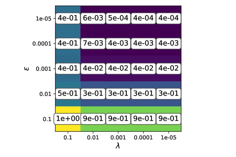
(a)

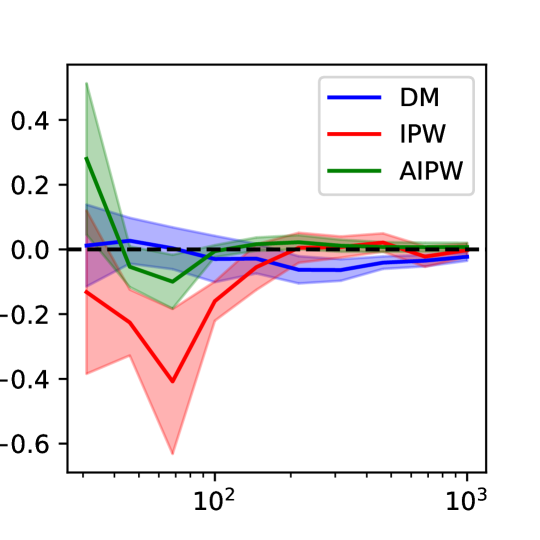
(b)

Figure 1: (a) Epsilon-lambda plot for mean potential outcome: MAE in approximation of one-step adjustment. (b) Error in estimation of $\mathbb{E}[Y(1)]$ over $n$.

8 Conclusions

We have presented a constructive algorithm that approximates Gateaux derivatives by finite differencing, with a focus on the statistical functionals used in causal inference and on stochastic optimization.

Regarding Q2 (the preservation of the beneficial statistical properties of estimators under numerical approximation), our analysis of different functionals surfaced fine-grained differences in opportunities for weakening requirements for computational approximation: Theorem 1 and Proposition 6 have different, estimand-dependent implications. Regarding Q3, we studied examples of causal estimands of recent interest in the literature that can be written as linear stochastic optimization functionals, and provided generic arguments for the non-parametric influence function, inspired by perturbation analysis of linear programs. The main insight is that unlike generic perturbation analysis of stochastic programs, which holds the optimal solution fixed when differentiating through the optimal value, obtaining influence functions requires to perturb the dependence of the solution on probability distribution primitives.

There are several directions which are natural follow-ups to this work. First, the smoothing perturbation, although it restores absolute continuity, introduces technical barriers in the implied approximation rates with regards to dimension dependence. Other arguments that reduce the dependence on smoothing would be of interest.

A useful direction would be to explore methods that are fully adaptive, not requiring any prior knowledge of beneficial statistical properties. Finally, our work has been mainly theoretical, and it would be useful to conduct further empirical comparisons of our approach based on numerical differentiation to various alternatives.

Acknowledgements.

Angela Zhou gratefully acknowledges support from the Foundations of Data Science Institute and the Simons Institute’s Program on Causality. Part of this work was done while the author was visiting the Simons Institute for the Theory of Computing. Yixin Wang acknowledges National Science Foundation Grant NSF-CHE-2231174. Michael Jordan acknowledges support from the Vannevar Bush Faculty Fellowship program under grant number N00014-21-1-2941.

Appendix A Overview and background for influence functions

For a broad overview of influence functions and their role in causal inference, see Tsiatis [2006], Hines et al. [2022], Kennedy [2022].

We focus on functionals that admit an asymptotically linear representation:

$$\Psi(\tilde{P})-\Psi(P) =-\int\phi(u;\tilde{P})dP(u)+R_{2}\left(\tilde{P},P\right),$$

where the influence function, $\phi(u;\tilde{P})$, captures the first-order bias in the functional. That is, we focus on functionals that are smooth enough to admit a von Mises expansion with a mean-zero, finite-variance influence function and a second-order remainder term $R_{2}\left(P_{1},P\right)$.

Appendix B Proofs for Section 4

B.0.1 Supplementary lemmas

Lemma 2 (Intermediate decomposition).

$$\frac{1}{\epsilon}\int\int y\left(\frac{\tilde{p}_{\epsilon}(y,A=1,x)}{\tilde{p}_{\epsilon}(A=1,x)}-\frac{\tilde{p}(y,A=1,x)}{\tilde{p}(A=1,x)}\right)\tilde{p}(x)\mathrm{d}y\;\mathrm{d}x$$

$$\qquad=\int\frac{\tilde{p}(x)}{\tilde{p}_{\epsilon}(A=1,x)}\mathbb{I}\left[a_{i}=1\right]\tilde{\delta}_{(x_{i})}^{\lambda}(x)\left\{\left(\int y\;\tilde{\delta}_{y_{i}}^{\lambda}(y)\mathrm{d}y\right)-\mathbb{E}_{\tilde{p}}[Y\mid A=1,x]\right\}\mathrm{d}x.$$

B.0.2 Proofs

Proof of Proposition 1.

We have:

$$\frac{\Psi(\tilde{P}_{\epsilon_{i}})-\Psi(\tilde{P})}{\epsilon} =\frac{1}{\epsilon}\int\left\{\int y\left[\frac{\tilde{p}_{\epsilon}(y,A=1,x)}{\tilde{p}_{\epsilon}(A=1,{x})}\left((1-\epsilon)\tilde{p}({x})+\epsilon\tilde{\delta}_{x_{{i}}}^{\lambda}\right)-\frac{\tilde{p}(y,A=1,x)}{\tilde{p}(A=1,x)}\tilde{p}(x)\right]\mathrm{d}y\right\}\mathrm{d}x$$

$$=\left[\int\tilde{p}(x)\int y\left(\frac{\tilde{p}_{\epsilon}(y,A=1,x)}{\tilde{p}_{\epsilon}(A=1,{x})}-\frac{\tilde{p}(y,A=1,x)}{\tilde{p}(A=1,x)}\right)\;\mathrm{d}y\;\mathrm{d}x\right]$$

$$\qquad+\cancel{\frac{1}{\epsilon}}\cancel{\epsilon}\int\int y\left[\frac{\tilde{p}_{\epsilon}(y,A=1,x)}{\tilde{p}_{\epsilon}(A=1,{x})}\tilde{\delta}_{x_{{i}}}^{\lambda}-\frac{\tilde{p}(y,A=1,x)}{\tilde{p}(A=1,x)}\tilde{p}(x)\right]\mathrm{d}y\;\mathrm{d}x.$$

The first term can be expanded using the decomposition of Lemma 2. We recognize the second term as $\left(\tilde{\mathbb{E}}_{\tilde{P}_{\epsilon}}[Y\mid A=1,X=x_{{i}}]-\Psi(\tilde{P})\right)$ by definition of the perturbed nuisances. We obtain:

$$\frac{\Psi(\tilde{P}_{\epsilon_{i}})-\Psi(\tilde{P})}{\epsilon} =(1-\epsilon)\int\tilde{p}(x)\int y\left(\frac{\tilde{p}_{\epsilon}(y,A=1,x)}{\tilde{p}_{\epsilon}(A=1,x)}-\frac{\tilde{p}(y,A=1,x)}{\tilde{p}(A=1,x)}\right)\mathrm{d}y\;\mathrm{d}x$$

$$=\int\frac{\tilde{p}(x)}{\tilde{p}_{\epsilon}(A=1,x)}\mathbb{I}\left[a_{i}=1\right]\tilde{\delta}_{x_{i}}^{\lambda}(x)\left\{\left(\int y\;\tilde{\delta}_{y_{i}}^{\lambda}(y)\mathrm{d}y\right)-\mathbb{E}_{\tilde{P}}[Y\mid A=1,x]\right\}\;\mathrm{d}x$$

$$\qquad+\left(\tilde{\mathbb{E}}_{\tilde{P}_{\epsilon}}[Y\mid A=1,X=x_{{i}}]-\Psi(\tilde{P})\right).$$

∎

Proof of Lemma 2.

Verify by direct computation.

For simplicity we consider a single summand in the sum (the claim follows by applying the same argument to every summand). Recall that ${\tilde{P}_{\epsilon}(A=1,X_{j})=(1-\epsilon)\tilde{p}(A=1,X_{j})+\epsilon\tilde{\mathbb{I}}\left[(o_{\backslash y})_{\tilde{{i}}}\right]}$ and expanding the latter yields:

$$\tilde{P}_{\epsilon}(A=1,X_{j})=\int\frac{\tilde{p}(x)}{\epsilon}\int y\left[\frac{(1-\epsilon)\tilde{p}(y,A=1,x)+\epsilon\tilde{\delta}_{o_{i}}^{\lambda}}{\tilde{p}_{\epsilon}(A=1,x)}-\frac{\tilde{p}(y,A=1,x)}{\tilde{p}(A=1,x)}\right]\mathrm{d}y\;\mathrm{d}x$$

$$=\int\frac{\tilde{p}(x)}{\epsilon}\int y\left[\frac{\left\{\cancel{(1-\epsilon)}\tilde{p}(y,A=1,x)+\epsilon\tilde{\delta}_{o_{i}}^{\lambda}\right\}\tilde{p}(A=1,x)}{\tilde{p}_{\epsilon}(A=1,x)\tilde{p}(A=1,x)}\right.$$

$$\qquad\qquad\qquad\qquad\left.-\frac{\tilde{p}(y,A=1,x)\left\{\cancel{(1-\epsilon)}\tilde{p}(A=1,x)+\epsilon\tilde{\delta}_{(a_{{i}},x_{{i}})}^{\lambda}\right\}}{\tilde{p}(A=1,x)\tilde{p}_{\epsilon}(A=1,x)}\right]\mathrm{d}y\;\mathrm{d}x$$

$$=\int\frac{\tilde{p}(x)}{\cancel{\epsilon}}\int y\left[\cancel{\epsilon}\frac{\tilde{\delta}_{o_{i}}^{\lambda}}{\tilde{p}_{\epsilon}(A=1,x)}-\cancel{\epsilon}\frac{\tilde{p}(y,A=1,x)\tilde{\delta}_{(a_{{i}},x_{{i}})}^{\lambda}}{\tilde{p}(A=1,x)\tilde{p}_{\epsilon}(A=1,x)}\right]\mathrm{d}y\;\mathrm{d}x$$

$$=\int\frac{\tilde{p}(x)}{\tilde{p}_{\epsilon}(A=1,x)}\tilde{\delta}_{(a_{{i}},x_{{i}})}^{\lambda}\;\left\{\int y{\tilde{\delta}_{y_{i}}^{\lambda}}\mathrm{d}y-\mathbb{E}_{\tilde{p}}[Y\mid A=1,x]\right\}\mathrm{d}x$$

$$=\int\frac{\tilde{p}(x)}{\tilde{p}_{\epsilon}(A=1,x)}\mathbb{I}\left[a_{i}=1\right]\tilde{\delta}_{(x_{i})}^{\lambda}(x)\;\left\{\int y{\tilde{\delta}_{y_{i}}^{\lambda}}\mathrm{d}y-\mathbb{E}_{\tilde{p}}[Y\mid A=1,x]\right\}\mathrm{d}x.$$

∎

Proof of Lemma 1.

To bound $\mathbb{E}[(\tilde{e}_{\epsilon}(X)-e(X))^{2}],$ argue similarly and observe that since $\tilde{e}_{\epsilon}=\tilde{p}_{\epsilon}(A=1\mid x)=\tilde{p}_{\epsilon}(A=1,{x})/\tilde{p}(x),$ we have:

$$\mathbb{E}[(\tilde{e}_{\epsilon}(X)-\tilde{e}(X))^{2}] =\int(((1-\epsilon)\tilde{p}(A=1,x)+\epsilon\tilde{\delta}_{a,X_{i}}^{\lambda}(x))-\tilde{p}(A=1,x))^{2}/\tilde{p}(x)^{2}\mathop{}\!\mathrm{d}x\cdot\tilde{p}(x)$$

$$=\epsilon^{2}\int(\tilde{\delta}_{a,X_{i}}^{\lambda}(x)-\tilde{p}(A=1,x))^{2}/\tilde{p}(x)\mathop{}\!\mathrm{d}x$$

$$=\epsilon^{2}\int((\tilde{\delta}_{a,X_{i}}^{\lambda}(x)^{2}-2\tilde{\delta}_{a,X_{i}}^{\lambda}(x)\tilde{p}(A=1,x)+\tilde{p}(A=1,x)^{2})/\tilde{p}(x)\mathop{}\!\mathrm{d}x$$

$$\leq\epsilon^{2}\int\nu(\tilde{\delta}_{a,X_{i}}^{\lambda}(x)^{2}+1)\mathop{}\!\mathrm{d}x$$

$$=\epsilon^{2}(\nu\lambda^{-d}R(\tilde{\delta}^{\lambda})+\nu)=O(\epsilon^{2}\lambda^{-d}).$$

In the second-to-last inequality we lower bound $\tilde{p}(x)\geq\nu$ and upper bound $\tilde{p}(A=1,x)\leq 1.$ In the last inequality we apply a change of variables to identify the term that arises in analysis of variance of kernel density estimates. We incur the $\lambda^{-d}$ dependence since we assumed that multivariate kernels are product kernels. The roughness term $R(\tilde{\delta}^{\lambda})=\int\tilde{\delta}^{2}{}(u)du$ depends on the particular $\tilde{\delta}$ kernel function and is a kernel-dependent constant. Hence the term scales overall as $\lambda^{-d}$ as in standard analyses of variance of kernel density estimates; see e.g. Ullah and Pagan [1999, pg. 23-26].

Next observe that:

$$\lVert\tilde{\mu}_{\epsilon}(X)-\mu(X)\rVert$$

$$\leq\lVert\tilde{\mu}_{\epsilon}(X)-\tilde{\mu}(X)\rVert+\lVert\tilde{\mu}(X)-\mu(X)\rVert$$

$$=\textstyle\left(\int\left\{\int\int y\left(\frac{(1-\epsilon)\tilde{p}(y,A=1,x^{\prime})+\epsilon\tilde{\delta}_{o}^{\lambda}}{(1-\epsilon)\tilde{p}(A=1,x^{\prime})+\epsilon\tilde{\delta}_{a,x}^{\lambda}}-\frac{\tilde{p}(y,A=1,x^{\prime})}{\tilde{p}(A=1,x^{\prime})}\right)\mathrm{d}y\mathrm{d}x^{\prime}\right\}^{2}p(x)\mathrm{d}x\right)^{\frac{1}{2}}+\lVert\tilde{\mu}(X)-\mu(X)\rVert$$

$$=\textstyle\left(\int\epsilon^{2}\left\{\frac{\tilde{p}(x)}{\tilde{p}_{\epsilon}(A=1,x)}\mathbb{I}\left[a_{i}=1\right]\tilde{\delta}_{(x_{i})}^{\lambda}(x)\left\{y_{i}-\mathbb{E}_{\tilde{p}}[Y\mid A=1,x]\right\}\right\}^{2}p(x)\mathrm{d}x\right)^{\frac{1}{2}}+\lVert\tilde{\mu}(X)-\mu(X)\rVert$$

$$=O(\epsilon\lambda^{-d/2})+\lVert\tilde{\mu}(X)-\mu(X)\rVert$$

where the first inequality comes from the triangle inequality, and the second equality from arguments similar to those in the previous bound. ∎

Proof of Theorem 1..

Let

$$\tilde{e}(X)=\tilde{p}(A=1,X)/\tilde{p}(X)=\tilde{p}(A=1\mid X),\tilde{\mu}(X)$$

denote the propensity and conditional outcome nuisances arising from plug-in estimation of $\tilde{P}$.

Let

$${\tilde{e}_{\epsilon}(X)=\tilde{p}_{\epsilon}(A=1\mid X)=\tilde{p}_{\epsilon}(A=1,X)}/{\tilde{p}(X)}$$

denote the nuisance arising from plug-in estimation at the perturbed distribution.

First observe that by Corollary 1:

$$\frac{\Psi(\tilde{P}_{\epsilon}^{{i}})-\Psi(\tilde{P})}{\epsilon} \textstyle=(1-\epsilon)\frac{\mathbb{I}\left[A_{i}=1\right]}{\tilde{p}_{\epsilon}(A=1\mid X_{i})}\left(Y_{i}-{\mathbb{E}_{\tilde{P}}[Y\mid A=1,X_{i}]}\right)+\left({\mathbb{E}}_{\tilde{P}_{\epsilon}}[Y\mid A=1,X_{{i}}]-\Psi(\tilde{P})\right)+O(\lambda^{J})$$

This decomposition characterizes convergence of an AIPW estimator with possibly biased but asymptotically consistent nuisances $\tilde{\mu},\tilde{e}_{\epsilon}$ in terms of the AIPW estimator with oracle nuisances—a standard analysis—and an additional term that vanishes on the order of $\epsilon$ (assuming strong overlap and boundedness). Define $\Gamma^{*}(O)$ as the doubly-robust score for AIPW with oracle nuisances $e^{*},\mu^{*}$, and let $\Gamma^{*}_{j}$ denote its empirical counterpart at $O_{j}=(X_{k},A_{k},Y_{k})$:

$$\Gamma^{*}(O)={\mathbb{I}\left[A=1\right]\frac{Y-\mu^{*}(X)}{e^{*}(X)}+\mu^{*}(X)}.$$

We will study the decomposition relative to the AIPW estimand with oracle nuisance estimates, with $\Gamma(O;e,\mu)$ denoting the above score but with nuisance functions $e,\mu$:

$$\Psi_{n}(\tilde{P})-\mathbb{E}[\Gamma^{*}(O;e^{*},\mu^{*})]$$

$$=\textstyle(\Psi(\tilde{P})+\frac{1}{n}\sum_{{{i}}=1}^{n}{{\tilde{\phi}}}_{{i}})-\mathbb{E}[\Gamma^{*}(O;e^{*},\mu^{*})]$$

$$=\mathbb{E}_{n}[\Gamma(O;\tilde{e}_{\epsilon},\tilde{\mu})]-\mathbb{E}[\Gamma^{*}(O;e^{*},\mu^{*})]+\mathbb{E}_{n}[\tilde{\mu}_{\epsilon}(X)-\tilde{\mu}(X)]+O(\lambda^{\beta})$$

$$=(\mathbb{E}_{n}-\mathbb{E})[\Gamma(O;\tilde{e}_{\epsilon},\tilde{\mu})]+\mathbb{E}[\Gamma(O;\tilde{e}_{\epsilon},\tilde{\mu})-\Gamma^{*}(O;e^{*},\mu^{*})]+\mathbb{E}_{n}[\tilde{\mu}_{\epsilon}(X)-\tilde{\mu}(X)]+O(\lambda^{\beta}),$$

where the second equality follows by Proposition 1, and the third by adding/subtracting $\mathbb{E}[\Gamma(O;\tilde{e}_{\epsilon},\tilde{\mu})].$

The first term, $(\mathbb{E}_{n}-\mathbb{E})[\Gamma(O;\tilde{e}_{\epsilon},\tilde{\mu})]$ is the standard empirical process term of the decomposition, obtained by the Donsker assumption and classical stability results for Donsker classes [Van der Vaart, 2000]:

$$(\mathbb{E}_{n}-\mathbb{E})[\Gamma(O;\tilde{e}_{\epsilon},\tilde{\mu})]={(\mathbb{E}_{n}-\mathbb{E})[\Gamma(O;{e}^{*},\mu^{*})]+o_{p}(n^{-\frac{1}{2}}).}$$

Hence, we have

$$\Psi_{n}(\tilde{P})-\mathbb{E}[\Gamma^{*}(O;e^{*},\mu^{*})]=\mathbb{E}[\Gamma(O;\tilde{e}_{\epsilon},\tilde{\mu})-\Gamma^{*}(O;e^{*},\mu^{*})]+\mathbb{E}_{n}[\tilde{\mu}_{\epsilon}(X)-\tilde{\mu}(X)]+O(\lambda^{\beta})+o_{p}(n^{-\frac{1}{2}}).$$ (15)

We obtain the product error conditions by standard decomposition of the remaining first term:

$$\mathbb{E}[\Gamma(O;\tilde{e}_{\epsilon},\tilde{\mu})-\Gamma^{*}(O;e^{*},\mu^{*})]$$

$$=\mathbb{E}\left[\left(\mathbb{I}\left[A=1\right]\frac{Y-\tilde{\mu}(X)}{\tilde{e}_{\epsilon}(X)}+\tilde{\mu}(X)\right)\right]-\mathbb{E}\left[\left(\mathbb{I}\left[A=1\right]\frac{Y-\mu^{*}(X)}{e^{*}(X)}+\mu^{*}(X)\right)\right]$$

$$=\mathbb{E}\left[\mathbb{I}\left[A=1\right]\left(\frac{1}{\tilde{e}_{\epsilon}(X)}-\frac{1}{e^{*}(X)}\right)(Y-\mu^{*}(X))\right]-\mathbb{E}\left[\left(\frac{1}{e^{*}(X)}-1\right)(\tilde{\mu}(X)-\mu^{*}(X))\right]$$

$$\qquad+\mathbb{E}\left[\mathbb{I}\left[A=1\right]\left(\frac{1}{\tilde{e}_{\epsilon}(X)}-\frac{1}{e^{*}(X)}\right)(\tilde{\mu}(X)-\mu^{*}(X))\right]$$

$$=\mathbb{E}\left[\mathbb{I}\left[A=1\right]\left(\frac{1}{\tilde{e}_{\epsilon}(X)}-\frac{1}{e^{*}(X)}\right)(\tilde{\mu}(X)-\mu^{*}(X))\right]$$

$$\leq\nu\|\tilde{e}_{\epsilon}(X)-{e^{*}(X)}\|_{2,P}\times\|\tilde{\mu}(X)-\mu^{*}(X)\|_{2,P}.$$

The second equality follows by adding/subtracting $\mathbb{I}\left[A=1\right]/\tilde{e}_{\epsilon},\mathbb{I}\left[A=1\right]\tilde{\mu}/e^{*},\mathbb{I}\left[A=1\right]\mu^{*}/e^{*}$). The third equality follows from iterated expectations. The last inequality follows from the Cauchy-Schwarz inequality and overlap. Therefore, $\epsilon$ must satisfy a rate so that $\tilde{e}_{\epsilon}$ converges at typical double robustness fast rates, such as $n^{-1/4}$, under a suitable sample splitting scheme.

For the last term of Equation 15, note that by Lemma 2, the numerical error $\epsilon$ is multiplied by error rate of the outcome nuisance:

$$\mathbb{E}[\tilde{\mu}_{\epsilon}(X)-\tilde{\mu}(X)] =\epsilon\int\int\frac{\tilde{p}(x)}{\tilde{p}_{\epsilon}(A=1,x)}\mathbb{I}\left[a_{i}=1\right]\tilde{\delta}_{(x_{i})}^{\lambda}(x)\;\left\{y_{i}-\mathbb{E}_{\tilde{p}}[Y\mid A=1,x]\right\}\mathrm{d}x$$

$$=\epsilon\;\mathbb{E}\left[\frac{\mathbb{I}\left[A=1\right]}{\tilde{p}_{\epsilon}(A=1\mid X)}\;\left\{Y-\mathbb{E}_{\tilde{p}}[Y\mid A=1,X]\right\}\right]+O(\lambda^{\beta})$$

$$\leq\|{\mathbb{I}\left[A=1\right]}/{\tilde{p}_{\epsilon}(A=1\mid X)}\|_{2,P}\|{Y-\mathbb{E}_{\tilde{p}}[Y\mid A=1,X]}\|_{2,P}+O(\lambda^{\beta})$$

$$=O(\lambda^{\beta})+O_{p}(n^{-r_{\mu}})\epsilon,$$

by application of Cauchy-Schwarz inequality and strong overlap. The claim follows by application of Lemma 1 to deduce implications on $\epsilon$ from standard product-error rate requirements on $\tilde{\mu},\tilde{e}$. ∎

Appendix C Proofs for Section 7

C.1 Empirical Gateaux derivative for multi-stage dynamic treatment regimes

We study the estimation properties of the empirical Gateaux derivative for multi-stage DTR from the probability density representation. In $T$-stage dynamic treatment regimes, the causal quantity of interest is the mean potential outcome $\mathbb{E}\left[Y^{\bar{a}}\right]$, where $\bar{a}=(a_{0},\ldots,a_{T})$ is the (deterministic) treatment strategy. Assuming $Y^{\bar{a}}$ is sequentially ignorable given treatment and covariate history $(\bar{A}_{t},\bar{X}_{t})$ at each time $t$, this causal quantity can be identified by the $g$-formula

$$\mathbb{E}\left[Y^{\bar{a}}\right]=\int\mathbb{E}\left[Y\,|\,\bar{A}=\bar{a},\bar{X}=\bar{x}\right]\prod_{t=1}^{T}\tilde{p}(x_{t}\,|\,\bar{a}_{t-1},\bar{x}_{t-1})\mathop{}\!\mathrm{d}\bar{x},$$

where $\bar{A}=(A_{0},\ldots,A_{t}),\bar{X}=(X_{0},\ldots,X_{t})$.

To derive its influence function, we take the empirical Gateaux derivative by considering the perturbation in the direction of $o_{i}=(\bar{x}_{i},\bar{a}_{i},y_{i})$, where $\bar{x}_{i}=(x_{i0},\ldots,x_{it})$ and $\bar{a}_{i}=(a_{i0},\ldots,a_{it})$:

$$\Psi(\tilde{P}^{i}_{\epsilon}) =\int\left(\int y\cdot\frac{\tilde{p}_{\epsilon}(y,\bar{A}=\bar{a},\bar{X}=\bar{x})}{\tilde{p}_{\epsilon}(\bar{A}=\bar{a},\bar{X}=\bar{x})}\mathop{}\!\mathrm{d}y\right)\prod_{t=1}^{T}\frac{\tilde{p}_{\epsilon}(x_{t},\bar{a}_{t-1},\bar{x}_{t-1})}{\tilde{p}_{\epsilon}(\bar{a}_{t-1},\bar{x}_{t-1}))}\cdot\tilde{p}_{\epsilon}(x_{0})\mathop{}\!\mathrm{d}\bar{x}.$$ (16)

Below we characterize how this empirical Gateaux derivative at the smoothed distribution differs from the one at the (unsmoothed) estimated distribution. The following result is analogous to Proposition 1 but is extended to the dynamic treatment regimes.

Proof of Proposition 2.

We first provide a more explicit statement of the result in Proposition 2.

$$\frac{\Psi(\tilde{P}^{i}_{\epsilon})-\Psi(\tilde{P})}{\epsilon}$$

$$=\left[\int\mathbb{E}_{\tilde{p}_{\epsilon}}\left[Y\,|\,\bar{A}=\bar{a},\bar{X}_{1:T}=\bar{x}_{1:T},X_{0}=x_{i0}\right]\prod_{t=1}^{T}\tilde{p}(x_{t}\,|\,\bar{a}_{t-1},\bar{x}_{1:t-1},x_{i0})\mathop{}\!\mathrm{d}\bar{x}-\Psi(\tilde{P})\right]$$

$$\quad+\int\tilde{p}(x_{0})\left\{\left[\frac{\tilde{\delta}^{\lambda}_{(\bar{a}_{i},\bar{x}_{i})}}{\tilde{p}_{\epsilon}(\bar{A}=\bar{a},\bar{X}=\bar{x})}{}\left[\int y\cdot\tilde{\delta}^{\lambda}_{y_{i}}\mathop{}\!\mathrm{d}y-\mathbb{E}_{\tilde{p}}\left[Y\,|\,\bar{A}=\bar{a},\bar{X}=\bar{x}\right]\right]\right]\prod_{t=1}^{T}\frac{\tilde{p}(x_{t},\bar{a}_{t-1},\bar{x}_{t-1})}{\tilde{p}(\bar{a}_{t-1},\bar{x}_{t-1}))}\right\}\mathop{}\!\mathrm{d}\bar{x}$$

$$\quad+\sum_{s=1}^{T}\int\tilde{p}(x_{0})\left\{\left(\int y\cdot\frac{\tilde{p}_{\epsilon}(y,\bar{A}=\bar{a},\bar{X}=\bar{x})}{\tilde{p}_{\epsilon}(\bar{A}=\bar{a},\bar{X}=\bar{x})}\mathop{}\!\mathrm{d}y\right)\left[\left\{\prod_{t=s+1}^{T}\frac{\tilde{p}(x_{t},\bar{a}_{t-1},\bar{x}_{t-1})}{\tilde{p}(\bar{a}_{t-1},\bar{x}_{t-1}))}\prod_{t=1}^{s-1}\frac{\tilde{p}_{\epsilon}(x_{t},\bar{a}_{t-1},\bar{x}_{t-1})}{\tilde{p}_{\epsilon}(\bar{a}_{t-1},\bar{x}_{t-1}))}\right.\right.\right.$$

$$\qquad\qquad\times\left.\left.\left.\frac{1}{\tilde{p}_{\epsilon}(\bar{a}_{s-1},\bar{x}_{s-1}))}\left[\tilde{\delta}^{\lambda}_{(\bar{a}_{i,s-1},\bar{x}_{i,s})})-\frac{\tilde{p}(x_{s},\bar{a}_{s-1},\bar{x}_{s-1})}{\tilde{p}(\bar{a}_{s-1},\bar{x}_{s-1}))}\tilde{\delta}^{\lambda}_{(\bar{a}_{i,s-1},\bar{x}_{i,s-1})}\right]\right\}\right]\right\}\mathop{}\!\mathrm{d}\bar{x}$$

$$\quad+\epsilon\sum_{s=1}^{T}\int\mathbb{E}_{\tilde{p}_{\epsilon}}\left[Y\,|\,\bar{A}=\bar{a},\bar{X}_{1:T}=\bar{x}_{1:T},X_{0}=x_{i0}\right]$$

$$\qquad\qquad\times\left[\left\{\prod_{t=s+1}^{T}\frac{\tilde{p}(x_{t},\bar{a}_{t-1},\bar{x}_{1:t-1},x_{i0})}{\tilde{p}(\bar{a}_{t-1},\bar{x}_{1:t-1},x_{i0}))}\prod_{t=1}^{s-1}\frac{\tilde{p}_{\epsilon}(x_{t},\bar{a}_{t-1},\bar{x}_{1:t-1},x_{i0})}{\tilde{p}_{\epsilon}(\bar{a}_{t-1},\bar{x}_{1:t-1},x_{i0}))}\frac{1}{\tilde{p}_{\epsilon}(\bar{a}_{s-1},\bar{x}_{1:s-1},x_{i0}))}\right.\right.$$

$$\qquad\qquad\qquad\qquad\times\left.\left.\left[\tilde{\delta}^{\lambda}_{(\bar{a}_{i,s-1},\bar{x}_{i,s})})-\frac{\tilde{p}(x_{s},\bar{a}_{s-1},\bar{x}_{1:s-1},x_{i0})}{\tilde{p}(\bar{a}_{s-1},\bar{x}_{1:s-1},x_{i0}))}\tilde{\delta}^{\lambda}_{(\bar{a}_{i,s-1},\bar{x}_{i,s-1})}\right]\right\}\right]\mathop{}\!\mathrm{d}\bar{x}.$$ (17)

For comparison, the exact efficient influence function under the non-Markovian dynamic treatment regime is

$$\left[\mathbb{E}_{\tilde{p}(\bar{x}_{1:T})}\left[\mathbb{E}_{\tilde{p}}\left[Y\,|\,\bar{A}=\bar{a},\bar{X}_{1:T}=\bar{x}_{1:T},X_{0}=x_{i0}\right]\right]-\Psi(\tilde{P})\right]$$

$$\quad+\frac{\mathbb{I}{(\bar{a}_{i})}}{\tilde{p}(\bar{A}=\bar{a}\,|\,\bar{X}=\bar{x})}{}\left[Y_{i}-\mathbb{E}_{\tilde{p}(\bar{x})}\left[\mathbb{E}_{\tilde{p}}\left[Y\,|\,\bar{A}=\bar{a},\bar{X}=\bar{x}\right]\right]\right]$$

$$\quad+\sum_{s=1}^{T}\frac{\mathbb{I}{(\bar{a}_{i,T-s},\bar{x}_{i,T-s+1})}}{\tilde{p}_{\epsilon}(\bar{a}_{T-s}\,|\,\bar{x}_{T-s})}\left[\int\mathbb{E}_{\tilde{p}}\left[Y\,|\,\bar{A}=\bar{a},\bar{X}=\bar{x}\right]{\prod_{t=T-s+1}^{T-1}\tilde{p}(x_{t}\,|\,\bar{a}_{t-1},\bar{x}_{t-1})\mathop{}\!\mathrm{d}\bar{x}_{(T-s+1):(T-1)}}\right]$$

$$\quad-\sum_{s=1}^{T}\frac{\mathbb{I}{(\bar{a}_{i,T-s},\bar{x}_{i,T-s})}}{\tilde{p}(\bar{a}_{T-s}\,|\,\bar{x}_{T-s})}\left[\int\mathbb{E}_{\tilde{p}}\left[Y\,|\,\bar{A}=\bar{a},\bar{X}=\bar{x}\right]\prod_{t=T-s}^{T-1}\tilde{p}(x_{t}\,|\,\bar{a}_{t-1},\bar{x}_{t-1})\mathop{}\!\mathrm{d}\bar{x}_{(T-s):(T-1)}\right].$$

This proposition performs a decomposition of the empirical derivative. It quantifies the additive bias due to the smoothed perturbation compared to the (raw) perturbation at the observation $o_{i}$.

We first decompose the empirical Gateaux derivative.

$$\frac{\Psi(\tilde{P}^{i}_{\epsilon})-\Psi(\tilde{P})}{\epsilon}$$

$$=\frac{1}{\epsilon}\left[\int\left(\int y\cdot\frac{\tilde{p}_{\epsilon}(y,\bar{A}=\bar{a},\bar{X}=\bar{x})}{\tilde{p}_{\epsilon}(\bar{A}=\bar{a},\bar{X}=\bar{x})}\mathop{}\!\mathrm{d}y\right)\prod_{t=1}^{T}\frac{\tilde{p}_{\epsilon}(x_{t},\bar{a}_{t-1},\bar{x}_{t-1})}{\tilde{p}_{\epsilon}(\bar{a}_{t-1},\bar{x}_{t-1}))}\cdot[(1-\epsilon)\tilde{p}(x_{0})+\epsilon\tilde{\delta}^{\lambda}_{x_{i0}}]\mathop{}\!\mathrm{d}\bar{x}\right.$$

$$\quad\left.-\int\left(\int y\cdot\frac{\tilde{p}(y,\bar{A}=\bar{a},\bar{X}=\bar{x})}{\tilde{p}(\bar{A}=\bar{a},\bar{X}=\bar{x})}\mathop{}\!\mathrm{d}y\right)\prod_{t=1}^{T}\frac{\tilde{p}(x_{t},\bar{a}_{t-1},\bar{x}_{t-1})}{\tilde{p}(\bar{a}_{t-1},\bar{x}_{t-1}))}\cdot\tilde{p}(x_{0})\mathop{}\!\mathrm{d}\bar{x}\right]$$ (18)

$$=\int\left[\left(\int y\cdot\frac{\tilde{p}_{\epsilon}(y,\bar{A}=\bar{a},\bar{X}=\bar{x})}{\tilde{p}_{\epsilon}(\bar{A}=\bar{a},\bar{X}=\bar{x})}\mathop{}\!\mathrm{d}y\right)\prod_{t=1}^{T}\frac{\tilde{p}_{\epsilon}(x_{t},\bar{a}_{t-1},\bar{x}_{t-1})}{\tilde{p}_{\epsilon}(\bar{a}_{t-1},\bar{x}_{t-1}))}\cdot\tilde{\delta}^{\lambda}_{x_{i0}}\right.$$

$$\quad-\left.\left(\int y\cdot\frac{\tilde{p}(y,\bar{A}=\bar{a},\bar{X}=\bar{x})}{\tilde{p}(\bar{A}=\bar{a},\bar{X}=\bar{x})}\mathop{}\!\mathrm{d}y\right)\prod_{t=1}^{T}\frac{\tilde{p}(x_{t},\bar{a}_{t-1},\bar{x}_{t-1})}{\tilde{p}(\bar{a}_{t-1},\bar{x}_{t-1}))}\cdot\tilde{p}(x_{0})\right]\mathop{}\!\mathrm{d}\bar{x}$$

$$\quad+\frac{1}{\epsilon}\left[\int\tilde{p}(x_{0})\left[\left(\int y\cdot\frac{\tilde{p}_{\epsilon}(y,\bar{A}=\bar{a},\bar{X}=\bar{x})}{\tilde{p}_{\epsilon}(\bar{A}=\bar{a},\bar{X}=\bar{x})}\mathop{}\!\mathrm{d}y\right)\prod_{t=1}^{T}\frac{\tilde{p}_{\epsilon}(x_{t},\bar{a}_{t-1},\bar{x}_{t-1})}{\tilde{p}_{\epsilon}(\bar{a}_{t-1},\bar{x}_{t-1}))}\right.\right.$$

$$\quad\left.\left.-\left(\int y\cdot\frac{\tilde{p}(y,\bar{A}=\bar{a},\bar{X}=\bar{x})}{\tilde{p}(\bar{A}=\bar{a},\bar{X}=\bar{x})}\mathop{}\!\mathrm{d}y\right)\prod_{t=1}^{T}\frac{\tilde{p}(x_{t},\bar{a}_{t-1},\bar{x}_{t-1})}{\tilde{p}(\bar{a}_{t-1},\bar{x}_{t-1})}\right]\mathop{}\!\mathrm{d}\bar{x}\right]$$ (19)

$$=\left[\int\mathbb{E}_{\tilde{p}_{\epsilon}}\left[Y\,|\,\bar{A}=\bar{a},\bar{X}_{T}=\bar{x}_{T}\right]\prod_{t=1}^{T}\tilde{p}_{\epsilon}(x_{t}\,|\,\bar{a}_{t-1},\bar{x}_{t-1})\tilde{p}(x_{0})\tilde{\delta}^{\lambda}_{x_{i0}}\mathop{}\!\mathrm{d}\bar{x}-\Psi(\tilde{P})\right]$$

$$\quad+\frac{1}{\epsilon}\left[\int\tilde{p}(x_{0})\left[\left(\int y\cdot\frac{\tilde{p}_{\epsilon}(y,\bar{A}=\bar{a},\bar{X}=\bar{x})}{\tilde{p}_{\epsilon}(\bar{A}=\bar{a},\bar{X}=\bar{x})}\mathop{}\!\mathrm{d}y\right)\prod_{t=1}^{T}\frac{\tilde{p}_{\epsilon}(x_{t},\bar{a}_{t-1},\bar{x}_{t-1})}{\tilde{p}_{\epsilon}(\bar{a}_{t-1},\bar{x}_{t-1}))}\right.\right.$$

$$\quad\left.\left.-\left(\int y\cdot\frac{\tilde{p}(y,\bar{A}=\bar{a},\bar{X}=\bar{x})}{\tilde{p}(\bar{A}=\bar{a},\bar{X}=\bar{x})}\mathop{}\!\mathrm{d}y\right)\prod_{t=1}^{T}\frac{\tilde{p}(x_{t},\bar{a}_{t-1},\bar{x}_{t-1})}{\tilde{p}(\bar{a}_{t-1},\bar{x}_{t-1}))}\right]\mathop{}\!\mathrm{d}\bar{x}\right]$$

$$=\left[\int\mathbb{E}_{\tilde{p}_{\epsilon}}\left[Y\,|\,\bar{A}=\bar{a},\bar{X}_{1:T}=\bar{x}_{1:T},X_{0}=x_{i0}\right]\prod_{t=1}^{T}\tilde{p}_{\epsilon}(x_{t}\,|\,\bar{a}_{t-1},\bar{x}_{1:t-1},x_{i0})\mathop{}\!\mathrm{d}\bar{x}-\Psi(\tilde{P})\right]$$

$$\quad+\frac{1}{\epsilon}\left[\int\tilde{p}(x_{0})\left[\left(\int y\cdot\frac{\tilde{p}_{\epsilon}(y,\bar{A}=\bar{a},\bar{X}=\bar{x})}{\tilde{p}_{\epsilon}(\bar{A}=\bar{a},\bar{X}=\bar{x})}\mathop{}\!\mathrm{d}y\right)\prod_{t=1}^{T}\frac{\tilde{p}_{\epsilon}(x_{t},\bar{a}_{t-1},\bar{x}_{t-1})}{\tilde{p}_{\epsilon}(\bar{a}_{t-1},\bar{x}_{t-1}))}\right.\right.$$

$$\quad\left.\left.-\left(\int y\cdot\frac{\tilde{p}(y,\bar{A}=\bar{a},\bar{X}=\bar{x})}{\tilde{p}(\bar{A}=\bar{a},\bar{X}=\bar{x})}\mathop{}\!\mathrm{d}y\right)\prod_{t=1}^{T}\frac{\tilde{p}(x_{t},\bar{a}_{t-1},\bar{x}_{t-1})}{\tilde{p}(\bar{a}_{t-1},\bar{x}_{t-1}))}\right]\mathop{}\!\mathrm{d}\bar{x}\right]$$ (20)

Equation 18 is due to the definition of the smoothed perturbation. Equation 19 separates the effect of smoothed perturbation into two pieces: the evaluation of $y$ and the evaluation of the density ratios. Equation 20 is due to the definition of $\mathbb{E}_{\tilde{p}_{\epsilon}}\left[\cdot\right]$.

Calculating the second term of Equation 20.

We first decompose this term into two difference terms:

$$\left(\int y\cdot\frac{\tilde{p}_{\epsilon}(y,\bar{A}=\bar{a},\bar{X}=\bar{x})}{\tilde{p}_{\epsilon}(\bar{A}=\bar{a},\bar{X}=\bar{x})}\mathop{}\!\mathrm{d}y\right)\prod_{t=1}^{T}\frac{\tilde{p}_{\epsilon}(x_{t},\bar{a}_{t-1},\bar{x}_{t-1})}{\tilde{p}_{\epsilon}(\bar{a}_{t-1},\bar{x}_{t-1}))}$$ (21)

$$\qquad\qquad-\left(\int y\cdot\frac{\tilde{p}(y,\bar{A}=\bar{a},\bar{X}=\bar{x})}{\tilde{p}(\bar{A}=\bar{a},\bar{X}=\bar{x})}\mathop{}\!\mathrm{d}y\right)\prod_{t=1}^{T}\frac{\tilde{p}(x_{t},\bar{a}_{t-1},\bar{x}_{t-1})}{\tilde{p}(\bar{a}_{t-1},\bar{x}_{t-1}))}$$

$$=\left(\int y\cdot\frac{\tilde{p}_{\epsilon}(y,\bar{A}=\bar{a},\bar{X}=\bar{x})}{\tilde{p}_{\epsilon}(\bar{A}=\bar{a},\bar{X}=\bar{x})}\mathop{}\!\mathrm{d}y\right)\left[\prod_{t=1}^{T}\frac{\tilde{p}_{\epsilon}(x_{t},\bar{a}_{t-1},\bar{x}_{t-1})}{\tilde{p}_{\epsilon}(\bar{a}_{t-1},\bar{x}_{t-1}))}-\prod_{t=1}^{T}\frac{\tilde{p}(x_{t},\bar{a}_{t-1},\bar{x}_{t-1})}{\tilde{p}(\bar{a}_{t-1},\bar{x}_{t-1}))}\right]$$

$$\quad+\left[\left(\int y\cdot\frac{\tilde{p}_{\epsilon}(y,\bar{A}=\bar{a},\bar{X}=\bar{x})}{\tilde{p}_{\epsilon}(\bar{A}=\bar{a},\bar{X}=\bar{x})}\mathop{}\!\mathrm{d}y\right)-\left(\int y\cdot\frac{\tilde{p}(y,\bar{A}=\bar{a},\bar{X}=\bar{x})}{\tilde{p}(\bar{A}=\bar{a},\bar{X}=\bar{x})}\mathop{}\!\mathrm{d}y\right)\right]\prod_{t=1}^{T}\frac{\tilde{p}(x_{t},\bar{a}_{t-1},\bar{x}_{t-1})}{\tilde{p}(\bar{a}_{t-1},\bar{x}_{t-1}))}.$$ (22)

The second difference term can be decomposed in a similar way as in Lemma 2.

$$\left(\int y\cdot\frac{\tilde{p}_{\epsilon}(y,\bar{A}=\bar{a},\bar{X}=\bar{x})}{\tilde{p}_{\epsilon}(\bar{A}=\bar{a},\bar{X}=\bar{x})}\mathop{}\!\mathrm{d}y\right)-\left(\int y\cdot\frac{\tilde{p}(y,\bar{A}=\bar{a},\bar{X}=\bar{x})}{\tilde{p}(\bar{A}=\bar{a},\bar{X}=\bar{x})}\mathop{}\!\mathrm{d}y\right)$$

$$=\int y\cdot\left[\frac{\tilde{p}_{\epsilon}(y,\bar{A}=\bar{a},\bar{X}=\bar{x})}{\tilde{p}_{\epsilon}(\bar{A}=\bar{a},\bar{X}=\bar{x})}-\frac{\tilde{p}(y,\bar{A}=\bar{a},\bar{X}=\bar{x})}{\tilde{p}(\bar{A}=\bar{a},\bar{X}=\bar{x})}\right]\mathop{}\!\mathrm{d}y$$

$$=\int y\cdot\left[\frac{(1-\epsilon)\tilde{p}(y,\bar{A}=\bar{a},\bar{X}=\bar{x})+\epsilon\tilde{\delta}^{\lambda}_{o_{i}}}{\tilde{p}_{\epsilon}(\bar{A}=\bar{a},\bar{X}=\bar{x})}-\frac{\tilde{p}(y,\bar{A}=\bar{a},\bar{X}=\bar{x})}{\tilde{p}(\bar{A}=\bar{a},\bar{X}=\bar{x})}\right]\mathop{}\!\mathrm{d}y$$

$$=\int y\cdot\left[\frac{((1-\epsilon)\tilde{p}(y,\bar{A}=\bar{a},\bar{X}=\bar{x})+\epsilon\tilde{\delta}^{\lambda}_{o_{i}})\tilde{p}(\bar{A}=\bar{a},\bar{X}=\bar{x})}{\tilde{p}_{\epsilon}(\bar{A}=\bar{a},\bar{X}=\bar{x})\tilde{p}(\bar{A}=\bar{a},\bar{X}=\bar{x})}\right.$$ (23)

$$\quad\quad\left.-\frac{\tilde{p}(y,\bar{A}=\bar{a},\bar{X}=\bar{x})((1-\epsilon)\tilde{p}(\bar{A}=\bar{a},\bar{X}=\bar{x})+\epsilon\tilde{\delta}^{\lambda}_{(\bar{a}_{i},\bar{x}_{i})})}{\tilde{p}_{\epsilon}(\bar{A}=\bar{a},\bar{X}=\bar{x})\tilde{p}(\bar{A}=\bar{a},\bar{X}=\bar{x})}\right]\mathop{}\!\mathrm{d}y$$

$$=\int y\cdot\left[\frac{(\epsilon\tilde{\delta}^{\lambda}_{o_{i}})\tilde{p}(\bar{A}=\bar{a},\bar{X}=\bar{x})}{\tilde{p}_{\epsilon}(\bar{A}=\bar{a},\bar{X}=\bar{x})\tilde{p}(\bar{A}=\bar{a},\bar{X}=\bar{x})}-\frac{\tilde{p}(y,\bar{A}=\bar{a},\bar{X}=\bar{x})(\epsilon\tilde{\delta}^{\lambda}_{(\bar{a}_{i},\bar{x}_{i})})}{\tilde{p}_{\epsilon}(\bar{A}=\bar{a},\bar{X}=\bar{x})\tilde{p}(\bar{A}=\bar{a},\bar{X}=\bar{x})}\right]\mathop{}\!\mathrm{d}y$$

$$=\frac{\epsilon\tilde{\delta}^{\lambda}_{(\bar{a}_{i},\bar{x}_{i})}}{\tilde{p}_{\epsilon}(\bar{A}=\bar{a},\bar{X}=\bar{x})}{}\int y\cdot\left[(\tilde{\delta}^{\lambda}_{y_{i}})-\frac{\tilde{p}(y,\bar{A}=\bar{a},\bar{X}=\bar{x})}{\tilde{p}(\bar{A}=\bar{a},\bar{X}=\bar{x})}\right]\mathop{}\!\mathrm{d}y$$

$$=\frac{\epsilon\tilde{\delta}^{\lambda}_{(\bar{a}_{i},\bar{x}_{i})}}{\tilde{p}_{\epsilon}(\bar{A}=\bar{a},\bar{X}=\bar{x})}{}\left[\int y\cdot\tilde{\delta}^{\lambda}_{y_{i}}\mathop{}\!\mathrm{d}y-\mathbb{E}_{\tilde{p}}\left[Y\,|\,\bar{A}=\bar{a},\bar{X}=\bar{x}\right]\right].$$

We next analyze the first difference term by induction:

$$\prod_{t=1}^{T}\frac{\tilde{p}_{\epsilon}(x_{t},\bar{a}_{t-1},\bar{x}_{t-1})}{\tilde{p}_{\epsilon}(\bar{a}_{t-1},\bar{x}_{t-1}))}-\prod_{t=1}^{T}\frac{\tilde{p}(x_{t},\bar{a}_{t-1},\bar{x}_{t-1})}{\tilde{p}(\bar{a}_{t-1},\bar{x}_{t-1}))}$$

$$=\prod_{t=1}^{T-1}\frac{\tilde{p}_{\epsilon}(x_{t},\bar{a}_{t-1},\bar{x}_{t-1})}{\tilde{p}_{\epsilon}(\bar{a}_{t-1},\bar{x}_{t-1}))}\left[\frac{\tilde{p}_{\epsilon}(x_{T},\bar{a}_{T-1},\bar{x}_{T-1})}{\tilde{p}_{\epsilon}(\bar{a}_{T-1},\bar{x}_{T-1}))}-\frac{\tilde{p}(x_{T},\bar{a}_{T-1},\bar{x}_{T-1})}{\tilde{p}(\bar{a}_{T-1},\bar{x}_{T-1}))}\right]$$

$$\quad+\frac{\tilde{p}(x_{T},\bar{a}_{T-1},\bar{x}_{T-1})}{\tilde{p}(\bar{a}_{T-1},\bar{x}_{T-1}))}\left[\prod_{t=1}^{T-1}\frac{\tilde{p}_{\epsilon}(x_{t},\bar{a}_{t-1},\bar{x}_{t-1})}{\tilde{p}_{\epsilon}(\bar{a}_{t-1},\bar{x}_{t-1}))}-\prod_{t=1}^{T-1}\frac{\tilde{p}(x_{t},\bar{a}_{t-1},\bar{x}_{t-1})}{\tilde{p}(\bar{a}_{t-1},\bar{x}_{t-1}))}\right].$$ (24)

Next we evaluate the key term in this induction $\frac{\tilde{p}_{\epsilon}(x_{s},\bar{a}_{s-1},\bar{x}_{s-1})}{\tilde{p}_{\epsilon}(\bar{a}_{s-1},\bar{x}_{s-1}))}-\frac{\tilde{p}(x_{s},\bar{a}_{s-1},\bar{x}_{s-1})}{\tilde{p}(\bar{a}_{s-1},\bar{x}_{s-1}))}$:

$$\frac{\tilde{p}_{\epsilon}(x_{s},\bar{a}_{s-1},\bar{x}_{s-1})}{\tilde{p}_{\epsilon}(\bar{a}_{s-1},\bar{x}_{s-1}))}-\frac{\tilde{p}(x_{s},\bar{a}_{s-1},\bar{x}_{s-1})}{\tilde{p}(\bar{a}_{s-1},\bar{x}_{s-1}))}$$

$$=\frac{((1-\epsilon)\tilde{p}(x_{s},\bar{a}_{s-1},\bar{x}_{s-1})+\epsilon\tilde{\delta}^{\lambda}_{o_{i}})\tilde{p}(\bar{a}_{s-1},\bar{x}_{s-1}))}{\tilde{p}_{\epsilon}(\bar{a}_{s-1},\bar{x}_{s-1}))\tilde{p}(\bar{a}_{s-1},\bar{x}_{s-1}))}-\frac{\tilde{p}(x_{s},\bar{a}_{s-1},\bar{x}_{s-1})((1-\epsilon)\tilde{p}(\bar{a}_{s-1},\bar{x}_{s-1}))+\epsilon\tilde{\delta}^{\lambda}_{o_{i}})}{\tilde{p}(\bar{a}_{s-1},\bar{x}_{s-1}))\tilde{p}_{\epsilon}(\bar{a}_{s-1},\bar{x}_{s-1}))}$$

$$=\frac{(\epsilon\tilde{\delta}^{\lambda}_{(\bar{a}_{i,s-1},\bar{x}_{i,s})})}{\tilde{p}_{\epsilon}(\bar{a}_{s-1},\bar{x}_{s-1}))}-\frac{\tilde{p}(x_{s},\bar{a}_{s-1},\bar{x}_{s-1})(\epsilon\tilde{\delta}^{\lambda}_{(\bar{a}_{i,s-1},\bar{x}_{i,s-1})})}{\tilde{p}(\bar{a}_{s-1},\bar{x}_{s-1}))\tilde{p}_{\epsilon}(\bar{a}_{s-1},\bar{x}_{s-1}))}$$

$$=\frac{\epsilon}{\tilde{p}_{\epsilon}(\bar{a}_{s-1},\bar{x}_{s-1}))}\left[\tilde{\delta}^{\lambda}_{(\bar{a}_{i,s-1},\bar{x}_{i,s})})-\frac{\tilde{p}(x_{s},\bar{a}_{s-1},\bar{x}_{s-1})}{\tilde{p}(\bar{a}_{s-1},\bar{x}_{s-1}))}\tilde{\delta}^{\lambda}_{(\bar{a}_{i,s-1},\bar{x}_{i,s-1})}\right].$$ (25)

Thus we have the following inductive relationship in $T$:

$$\prod_{t=1}^{T}\frac{\tilde{p}_{\epsilon}(x_{t},\bar{a}_{t-1},\bar{x}_{t-1})}{\tilde{p}_{\epsilon}(\bar{a}_{t-1},\bar{x}_{t-1}))}-\prod_{t=1}^{T}\frac{\tilde{p}(x_{t},\bar{a}_{t-1},\bar{x}_{t-1})}{\tilde{p}(\bar{a}_{t-1},\bar{x}_{t-1}))}$$

$$=\prod_{t=1}^{T-1}\frac{\tilde{p}_{\epsilon}(x_{t},\bar{a}_{t-1},\bar{x}_{t-1})}{\tilde{p}_{\epsilon}(\bar{a}_{t-1},\bar{x}_{t-1}))}\frac{\epsilon}{\tilde{p}_{\epsilon}(\bar{a}_{T-1},\bar{x}_{T-1}))}\left[\tilde{\delta}^{\lambda}_{(\bar{a}_{i,T-1},\bar{x}_{i,T})})-\frac{\tilde{p}(x_{T},\bar{a}_{T-1},\bar{x}_{T-1})}{\tilde{p}(\bar{a}_{T-1},\bar{x}_{T-1}))}\tilde{\delta}^{\lambda}_{(\bar{a}_{i,T-1},\bar{x}_{i,T-1})}\right]$$

$$\quad+\frac{\tilde{p}(x_{T},\bar{a}_{T-1},\bar{x}_{T-1})}{\tilde{p}(\bar{a}_{T-1},\bar{x}_{T-1}))}\left[\prod_{t=1}^{T-1}\frac{\tilde{p}_{\epsilon}(x_{t},\bar{a}_{t-1},\bar{x}_{t-1})}{\tilde{p}_{\epsilon}(\bar{a}_{t-1},\bar{x}_{t-1}))}-\prod_{t=1}^{T-1}\frac{\tilde{p}(x_{t},\bar{a}_{t-1},\bar{x}_{t-1})}{\tilde{p}(\bar{a}_{t-1},\bar{x}_{t-1}))}\right]$$ (26)

$$=\sum_{s=T-1}^{T}\left\{\prod_{t=s+1}^{T}\frac{\tilde{p}(x_{t},\bar{a}_{t-1},\bar{x}_{t-1})}{\tilde{p}(\bar{a}_{t-1},\bar{x}_{t-1}))}\prod_{t=1}^{s-1}\frac{\tilde{p}_{\epsilon}(x_{t},\bar{a}_{t-1},\bar{x}_{t-1})}{\tilde{p}_{\epsilon}(\bar{a}_{t-1},\bar{x}_{t-1}))}\frac{\epsilon}{\tilde{p}_{\epsilon}(\bar{a}_{s-1},\bar{x}_{s-1}))}\right.$$

$$\qquad\left.\qquad\times\left[\tilde{\delta}^{\lambda}_{(\bar{a}_{i,s-1},\bar{x}_{i,s})})-\frac{\tilde{p}(x_{s},\bar{a}_{s-1},\bar{x}_{s-1})}{\tilde{p}(\bar{a}_{s-1},\bar{x}_{s-1}))}\tilde{\delta}^{\lambda}_{(\bar{a}_{i,s-1},\bar{x}_{i,s-1})}\right]\right\}$$

$$\quad+\prod_{t=T-1}^{T}\frac{\tilde{p}(x_{t},\bar{a}_{t-1},\bar{x}_{t-1})}{\tilde{p}(\bar{a}_{t-1},\bar{x}_{t-1}))}\left[\prod_{t=1}^{T-2}\frac{\tilde{p}_{\epsilon}(x_{t},\bar{a}_{t-1},\bar{x}_{t-1})}{\tilde{p}_{\epsilon}(\bar{a}_{t-1},\bar{x}_{t-1}))}-\prod_{t=1}^{T-2}\frac{\tilde{p}(x_{t},\bar{a}_{t-1},\bar{x}_{t-1})}{\tilde{p}(\bar{a}_{t-1},\bar{x}_{t-1}))}\right]$$ (27)

$$=\sum_{s=1}^{T}\left\{\prod_{t=s+1}^{T}\frac{\tilde{p}(x_{t},\bar{a}_{t-1},\bar{x}_{t-1})}{\tilde{p}(\bar{a}_{t-1},\bar{x}_{t-1}))}\prod_{t=1}^{s-1}\frac{\tilde{p}_{\epsilon}(x_{t},\bar{a}_{t-1},\bar{x}_{t-1})}{\tilde{p}_{\epsilon}(\bar{a}_{t-1},\bar{x}_{t-1}))}\frac{\epsilon}{\tilde{p}_{\epsilon}(\bar{a}_{s-1},\bar{x}_{s-1}))}\right.$$

$$\qquad\qquad\times\left.\left[\tilde{\delta}^{\lambda}_{(\bar{a}_{i,s-1},\bar{x}_{i,s})})-\frac{\tilde{p}(x_{s},\bar{a}_{s-1},\bar{x}_{s-1})}{\tilde{p}(\bar{a}_{s-1},\bar{x}_{s-1}))}\tilde{\delta}^{\lambda}_{(\bar{a}_{i,s-1},\bar{x}_{i,s-1})}\right]\right\}.$$ (28)

These calculations imply that

$$\frac{\Psi(\tilde{P}^{i}_{\epsilon})-\Psi(\tilde{P})}{\epsilon}$$

$$=\left[\int\mathbb{E}_{\tilde{p}_{\epsilon}}\left[Y\,|\,\bar{A}=\bar{a},\bar{X}_{1:T}=\bar{x}_{1:T},X_{0}=x_{i0}\right]\prod_{t=1}^{T}\tilde{p}_{\epsilon}(x_{t}\,|\,\bar{a}_{t-1},\bar{x}_{1:t-1},x_{i0})\mathop{}\!\mathrm{d}\bar{x}-\Psi(\tilde{P})\right]$$

$$\quad+\frac{1}{\epsilon}\left[\int\tilde{p}(x_{0})\left[\left(\int y\cdot\frac{\tilde{p}_{\epsilon}(y,\bar{A}=\bar{a},\bar{X}=\bar{x})}{\tilde{p}_{\epsilon}(\bar{A}=\bar{a},\bar{X}=\bar{x})}\mathop{}\!\mathrm{d}y\right)\prod_{t=1}^{T}\frac{\tilde{p}_{\epsilon}(x_{t},\bar{a}_{t-1},\bar{x}_{t-1})}{\tilde{p}_{\epsilon}(\bar{a}_{t-1},\bar{x}_{t-1}))}\right.\right.$$

$$\quad\left.\left.-\left(\int y\cdot\frac{\tilde{p}(y,\bar{A}=\bar{a},\bar{X}=\bar{x})}{\tilde{p}(\bar{A}=\bar{a},\bar{X}=\bar{x})}\mathop{}\!\mathrm{d}y\right)\prod_{t=1}^{T}\frac{\tilde{p}(x_{t},\bar{a}_{t-1},\bar{x}_{t-1})}{\tilde{p}(\bar{a}_{t-1},\bar{x}_{t-1}))}\right]\mathop{}\!\mathrm{d}\bar{x}\right]$$ (29)

$$=\left[\int\mathbb{E}_{\tilde{p}_{\epsilon}}\left[Y\,|\,\bar{A}=\bar{a},\bar{X}_{1:T}=\bar{x}_{1:T},X_{0}=x_{i0}\right]\prod_{t=1}^{T}\tilde{p}_{\epsilon}(x_{t}\,|\,\bar{a}_{t-1},\bar{x}_{1:t-1},x_{i0})\mathop{}\!\mathrm{d}\bar{x}-\Psi(\tilde{P})\right]$$

$$\quad+\frac{1}{\epsilon}\int\tilde{p}(x_{0})\left\{\left(\int y\cdot\frac{\tilde{p}_{\epsilon}(y,\bar{A}=\bar{a},\bar{X}=\bar{x})}{\tilde{p}_{\epsilon}(\bar{A}=\bar{a},\bar{X}=\bar{x})}\mathop{}\!\mathrm{d}y\right)\left[\prod_{t=1}^{T}\frac{\tilde{p}_{\epsilon}(x_{t},\bar{a}_{t-1},\bar{x}_{t-1})}{\tilde{p}_{\epsilon}(\bar{a}_{t-1},\bar{x}_{t-1}))}-\prod_{t=1}^{T}\frac{\tilde{p}(x_{t},\bar{a}_{t-1},\bar{x}_{t-1})}{\tilde{p}(\bar{a}_{t-1},\bar{x}_{t-1}))}\right]\right.$$

$$\quad+\left.\left[\left(\int y\cdot\frac{\tilde{p}_{\epsilon}(y,\bar{A}=\bar{a},\bar{X}=\bar{x})}{\tilde{p}_{\epsilon}(\bar{A}=\bar{a},\bar{X}=\bar{x})}\mathop{}\!\mathrm{d}y\right)-\left(\int y\cdot\frac{\tilde{p}(y,\bar{A}=\bar{a},\bar{X}=\bar{x})}{\tilde{p}(\bar{A}=\bar{a},\bar{X}=\bar{x})}\mathop{}\!\mathrm{d}y\right)\right]\prod_{t=1}^{T}\frac{\tilde{p}(x_{t},\bar{a}_{t-1},\bar{x}_{t-1})}{\tilde{p}(\bar{a}_{t-1},\bar{x}_{t-1}))}\right\}\mathop{}\!\mathrm{d}\bar{x}$$ (30)

$$=\left[\int\mathbb{E}_{\tilde{p}_{\epsilon}}\left[Y\,|\,\bar{A}=\bar{a},\bar{X}_{1:T}=\bar{x}_{1:T},X_{0}=x_{i0}\right]\prod_{t=1}^{T}\tilde{p}_{\epsilon}(x_{t}\,|\,\bar{a}_{t-1},\bar{x}_{1:t-1},x_{i0})\mathop{}\!\mathrm{d}\bar{x}-\Psi(\tilde{P})\right]$$

$$\quad+\frac{1}{\epsilon}\int\tilde{p}(x_{0})\left\{\left(\int y\cdot\frac{\tilde{p}_{\epsilon}(y,\bar{A}=\bar{a},\bar{X}=\bar{x})}{\tilde{p}_{\epsilon}(\bar{A}=\bar{a},\bar{X}=\bar{x})}\mathop{}\!\mathrm{d}y\right)\left[\prod_{t=1}^{T}\frac{\tilde{p}_{\epsilon}(x_{t},\bar{a}_{t-1},\bar{x}_{t-1})}{\tilde{p}_{\epsilon}(\bar{a}_{t-1},\bar{x}_{t-1}))}-\prod_{t=1}^{T}\frac{\tilde{p}(x_{t},\bar{a}_{t-1},\bar{x}_{t-1})}{\tilde{p}(\bar{a}_{t-1},\bar{x}_{t-1}))}\right]\right\}\mathop{}\!\mathrm{d}\bar{x}$$

$$\quad+\frac{1}{\epsilon}\int\tilde{p}(x_{0})\left\{\left[\frac{\epsilon\tilde{\delta}^{\lambda}_{(\bar{a}_{i},\bar{x}_{i})}}{\tilde{p}_{\epsilon}(\bar{A}=\bar{a},\bar{X}=\bar{x})}{}\left[\int y\cdot\tilde{\delta}^{\lambda}_{y_{i}}\mathop{}\!\mathrm{d}y-\mathbb{E}_{\tilde{p}}\left[Y\,|\,\bar{A}=\bar{a},\bar{X}=\bar{x}\right]\right]\right]\prod_{t=1}^{T}\frac{\tilde{p}(x_{t},\bar{a}_{t-1},\bar{x}_{t-1})}{\tilde{p}(\bar{a}_{t-1},\bar{x}_{t-1}))}\right\}\mathop{}\!\mathrm{d}\bar{x}$$ (31)

$$=\left[\int\mathbb{E}_{\tilde{p}_{\epsilon}}\left[Y\,|\,\bar{A}=\bar{a},\bar{X}_{1:T}=\bar{x}_{1:T},X_{0}=x_{i0}\right]\prod_{t=1}^{T}\tilde{p}_{\epsilon}(x_{t}\,|\,\bar{a}_{t-1},\bar{x}_{1:t-1},x_{i0})\mathop{}\!\mathrm{d}\bar{x}-\Psi(\tilde{P})\right]$$

$$\quad+\frac{1}{\epsilon}\int\tilde{p}(x_{0})\left\{\left(\int y\cdot\frac{\tilde{p}_{\epsilon}(y,\bar{A}=\bar{a},\bar{X}=\bar{x})}{\tilde{p}_{\epsilon}(\bar{A}=\bar{a},\bar{X}=\bar{x})}\mathop{}\!\mathrm{d}y\right)\left[\sum_{s=1}^{T}\left\{\prod_{t=s+1}^{T}\frac{\tilde{p}(x_{t},\bar{a}_{t-1},\bar{x}_{t-1})}{\tilde{p}(\bar{a}_{t-1},\bar{x}_{t-1}))}\prod_{t=1}^{s-1}\frac{\tilde{p}_{\epsilon}(x_{t},\bar{a}_{t-1},\bar{x}_{t-1})}{\tilde{p}_{\epsilon}(\bar{a}_{t-1},\bar{x}_{t-1}))}\right.\right.\right.$$

$$\qquad\qquad\times\left.\left.\left.\frac{\epsilon}{\tilde{p}_{\epsilon}(\bar{a}_{s-1},\bar{x}_{s-1}))}\left[\tilde{\delta}^{\lambda}_{(\bar{a}_{i,s-1},\bar{x}_{i,s})})-\frac{\tilde{p}(x_{s},\bar{a}_{s-1},\bar{x}_{s-1})}{\tilde{p}(\bar{a}_{s-1},\bar{x}_{s-1}))}\tilde{\delta}^{\lambda}_{(\bar{a}_{i,s-1},\bar{x}_{i,s-1})}\right]\right\}\right]\right\}\mathop{}\!\mathrm{d}\bar{x}$$

$$\quad+\frac{1}{\epsilon}\int\tilde{p}(x_{0})\left\{\left[\frac{\epsilon\tilde{\delta}^{\lambda}_{(\bar{a}_{i},\bar{x}_{i})}}{\tilde{p}_{\epsilon}(\bar{A}=\bar{a},\bar{X}=\bar{x})}{}\left[\int y\cdot\tilde{\delta}^{\lambda}_{y_{i}}\mathop{}\!\mathrm{d}y-\mathbb{E}_{\tilde{p}}\left[Y\,|\,\bar{A}=\bar{a},\bar{X}=\bar{x}\right]\right]\right]\prod_{t=1}^{T}\frac{\tilde{p}(x_{t},\bar{a}_{t-1},\bar{x}_{t-1})}{\tilde{p}(\bar{a}_{t-1},\bar{x}_{t-1}))}\right\}\mathop{}\!\mathrm{d}\bar{x}$$ (32)

$$=\left[\int\mathbb{E}_{\tilde{p}_{\epsilon}}\left[Y\,|\,\bar{A}=\bar{a},\bar{X}_{1:T}=\bar{x}_{1:T},X_{0}=x_{i0}\right]\prod_{t=1}^{T}\tilde{p}_{\epsilon}(x_{t}\,|\,\bar{a}_{t-1},\bar{x}_{1:t-1},x_{i0})\mathop{}\!\mathrm{d}\bar{x}-\Psi(\tilde{P})\right]$$

$$\quad+\int\tilde{p}(x_{0})\left\{\left(\int y\cdot\frac{\tilde{p}_{\epsilon}(y,\bar{A}=\bar{a},\bar{X}=\bar{x})}{\tilde{p}_{\epsilon}(\bar{A}=\bar{a},\bar{X}=\bar{x})}\mathop{}\!\mathrm{d}y\right)\left[\sum_{s=1}^{T}\left\{\prod_{t=s+1}^{T}\frac{\tilde{p}(x_{t},\bar{a}_{t-1},\bar{x}_{t-1})}{\tilde{p}(\bar{a}_{t-1},\bar{x}_{t-1}))}\prod_{t=1}^{s-1}\frac{\tilde{p}_{\epsilon}(x_{t},\bar{a}_{t-1},\bar{x}_{t-1})}{\tilde{p}_{\epsilon}(\bar{a}_{t-1},\bar{x}_{t-1}))}\right.\right.\right.$$

$$\qquad\qquad\times\left.\left.\left.\frac{1}{\tilde{p}_{\epsilon}(\bar{a}_{s-1},\bar{x}_{s-1}))}\left[\tilde{\delta}^{\lambda}_{(\bar{a}_{i,s-1},\bar{x}_{i,s})})-\frac{\tilde{p}(x_{s},\bar{a}_{s-1},\bar{x}_{s-1})}{\tilde{p}(\bar{a}_{s-1},\bar{x}_{s-1}))}\tilde{\delta}^{\lambda}_{(\bar{a}_{i,s-1},\bar{x}_{i,s-1})}\right]\right\}\right]\right\}\mathop{}\!\mathrm{d}\bar{x}$$

$$\quad+\int\tilde{p}(x_{0})\left\{\left[\frac{\tilde{\delta}^{\lambda}_{(\bar{a}_{i},\bar{x}_{i})}}{\tilde{p}_{\epsilon}(\bar{A}=\bar{a},\bar{X}=\bar{x})}{}\left[\int y\cdot\tilde{\delta}^{\lambda}_{y_{i}}\mathop{}\!\mathrm{d}y-\mathbb{E}_{\tilde{p}}\left[Y\,|\,\bar{A}=\bar{a},\bar{X}=\bar{x}\right]\right]\right]\prod_{t=1}^{T}\frac{\tilde{p}(x_{t},\bar{a}_{t-1},\bar{x}_{t-1})}{\tilde{p}(\bar{a}_{t-1},\bar{x}_{t-1}))}\right\}\mathop{}\!\mathrm{d}\bar{x}.$$ (33)

Calculating the first term of Equation 33.

The first term of Equation 33 can be decomposed as follows:

$$\int\mathbb{E}_{\tilde{p}_{\epsilon}}\left[Y\,|\,\bar{A}=\bar{a},\bar{X}_{1:T}=\bar{x}_{1:T},X_{0}=x_{i0}\right]\prod_{t=1}^{T}\tilde{p}_{\epsilon}(x_{t}\,|\,\bar{a}_{t-1},\bar{x}_{1:t-1},x_{i0})\mathop{}\!\mathrm{d}\bar{x}$$

$$=\int\mathbb{E}_{\tilde{p}_{\epsilon}}\left[Y\,|\,\bar{A}=\bar{a},\bar{X}_{1:T}=\bar{x}_{1:T},X_{0}=x_{i0}\right]\prod_{t=1}^{T}\tilde{p}(x_{t}\,|\,\bar{a}_{t-1},\bar{x}_{1:t-1},x_{i0})\mathop{}\!\mathrm{d}\bar{x}$$ (34)

$$\qquad+\int\mathbb{E}_{\tilde{p}_{\epsilon}}\left[Y\,|\,\bar{A}=\bar{a},\bar{X}_{1:T}=\bar{x}_{1:T},X_{0}=x_{i0}\right]$$

$$\qquad\qquad\times\left[\prod_{t=1}^{T}\frac{\tilde{p}_{\epsilon}(x_{t},\bar{a}_{t-1},\bar{x}_{1:t-1},x_{i0})}{\tilde{p}_{\epsilon}(\bar{a}_{t-1},\bar{x}_{1:t-1},x_{i0}))}-\prod_{t=1}^{T}\frac{\tilde{p}(x_{t},\bar{a}_{t-1},\bar{x}_{1:t-1},x_{i0})}{\tilde{p}(\bar{a}_{t-1},\bar{x}_{1:t-1},x_{i0}))}\right]\mathop{}\!\mathrm{d}\bar{x}$$ (35)

Following a similar calculation as in Equation 28, we have that

$$\prod_{t=1}^{T}\frac{\tilde{p}_{\epsilon}(x_{t},\bar{a}_{t-1},\bar{x}_{1:t-1},x_{i0})}{\tilde{p}_{\epsilon}(\bar{a}_{t-1},\bar{x}_{1:t-1},x_{i0}))}-\prod_{t=1}^{T}\frac{\tilde{p}(x_{t},\bar{a}_{t-1},\bar{x}_{1:t-1},x_{i0})}{\tilde{p}(\bar{a}_{t-1},\bar{x}_{1:t-1},x_{i0}))}$$ (36)

$$=\sum_{s=1}^{T}\left\{\prod_{t=s+1}^{T}\frac{\tilde{p}(x_{t},\bar{a}_{t-1},\bar{x}_{1:t-1},x_{i0})}{\tilde{p}(\bar{a}_{t-1},\bar{x}_{1:t-1},x_{i0}))}\prod_{t=1}^{s-1}\frac{\tilde{p}_{\epsilon}(x_{t},\bar{a}_{t-1},\bar{x}_{1:t-1},x_{i0})}{\tilde{p}_{\epsilon}(\bar{a}_{t-1},\bar{x}_{1:t-1},x_{i0}))}\frac{\epsilon}{\tilde{p}_{\epsilon}(\bar{a}_{s-1},\bar{x}_{1:s-1},x_{i0}))}\right.$$

$$\qquad\qquad\times\left.\left[\tilde{\delta}^{\lambda}_{(\bar{a}_{i,s-1},\bar{x}_{i,s})})-\frac{\tilde{p}(x_{s},\bar{a}_{s-1},\bar{x}_{1:s-1},x_{i0})}{\tilde{p}(\bar{a}_{s-1},\bar{x}_{1:s-1},x_{i0}))}\tilde{\delta}^{\lambda}_{(\bar{a}_{i,s-1},\bar{x}_{i,s-1})}\right]\right\}$$ (37)

Thus the first term of Equation 33 is

$$\int\mathbb{E}_{\tilde{p}_{\epsilon}}\left[Y\,|\,\bar{A}=\bar{a},\bar{X}_{1:T}=\bar{x}_{1:T},X_{0}=x_{i0}\right]\prod_{t=1}^{T}\tilde{p}_{\epsilon}(x_{t}\,|\,\bar{a}_{t-1},\bar{x}_{1:t-1},x_{i0})\mathop{}\!\mathrm{d}\bar{x}$$

$$=\int\mathbb{E}_{\tilde{p}_{\epsilon}}\left[Y\,|\,\bar{A}=\bar{a},\bar{X}_{1:T}=\bar{x}_{1:T},X_{0}=x_{i0}\right]\prod_{t=1}^{T}\tilde{p}(x_{t}\,|\,\bar{a}_{t-1},\bar{x}_{1:t-1},x_{i0})\mathop{}\!\mathrm{d}\bar{x}$$ (38)

$$\qquad+\int\mathbb{E}_{\tilde{p}_{\epsilon}}\left[Y\,|\,\bar{A}=\bar{a},\bar{X}_{1:T}=\bar{x}_{1:T},X_{0}=x_{i0}\right]$$ (39)

$$\qquad\qquad\times\left[\sum_{s=1}^{T}\left\{\prod_{t=s+1}^{T}\frac{\tilde{p}(x_{t},\bar{a}_{t-1},\bar{x}_{1:t-1},x_{i0})}{\tilde{p}(\bar{a}_{t-1},\bar{x}_{1:t-1},x_{i0}))}\prod_{t=1}^{s-1}\frac{\tilde{p}_{\epsilon}(x_{t},\bar{a}_{t-1},\bar{x}_{1:t-1},x_{i0})}{\tilde{p}_{\epsilon}(\bar{a}_{t-1},\bar{x}_{1:t-1},x_{i0}))}\right.\right.$$

$$\qquad\qquad\times\left.\left.\frac{\epsilon}{\tilde{p}_{\epsilon}(\bar{a}_{s-1},\bar{x}_{1:s-1},x_{i0}))}\left[\tilde{\delta}^{\lambda}_{(\bar{a}_{i,s-1},\bar{x}_{i,s})})-\frac{\tilde{p}(x_{s},\bar{a}_{s-1},\bar{x}_{1:s-1},x_{i0})}{\tilde{p}(\bar{a}_{s-1},\bar{x}_{1:s-1},x_{i0}))}\tilde{\delta}^{\lambda}_{(\bar{a}_{i,s-1},\bar{x}_{i,s-1})}\right]\right\}\right]\mathop{}\!\mathrm{d}\bar{x}$$ (40)

Plugging this calculation into $\frac{\Psi(\tilde{P}^{i}_{\epsilon})-\Psi(\tilde{P})}{\epsilon}:$

$$\frac{\Psi(\tilde{P}^{i}_{\epsilon})-\Psi(\tilde{P})}{\epsilon}$$

$$=\left[\int\mathbb{E}_{\tilde{p}_{\epsilon}}\left[Y\,|\,\bar{A}=\bar{a},\bar{X}_{1:T}=\bar{x}_{1:T},X_{0}=x_{i0}\right]\prod_{t=1}^{T}\tilde{p}_{\epsilon}(x_{t}\,|\,\bar{a}_{t-1},\bar{x}_{1:t-1},x_{i0})\mathop{}\!\mathrm{d}\bar{x}-\Psi(\tilde{P})\right]$$

$$\quad+\int\tilde{p}(x_{0})\left\{\left(\int y\cdot\frac{\tilde{p}_{\epsilon}(y,\bar{A}=\bar{a},\bar{X}=\bar{x})}{\tilde{p}_{\epsilon}(\bar{A}=\bar{a},\bar{X}=\bar{x})}\mathop{}\!\mathrm{d}y\right)\left[\sum_{s=1}^{T}\left\{\prod_{t=s+1}^{T}\frac{\tilde{p}(x_{t},\bar{a}_{t-1},\bar{x}_{t-1})}{\tilde{p}(\bar{a}_{t-1},\bar{x}_{t-1}))}\prod_{t=1}^{s-1}\frac{\tilde{p}_{\epsilon}(x_{t},\bar{a}_{t-1},\bar{x}_{t-1})}{\tilde{p}_{\epsilon}(\bar{a}_{t-1},\bar{x}_{t-1}))}\right.\right.\right.$$

$$\qquad\qquad\times\left.\left.\left.\frac{1}{\tilde{p}_{\epsilon}(\bar{a}_{s-1},\bar{x}_{s-1}))}\left[\tilde{\delta}^{\lambda}_{(\bar{a}_{i,s-1},\bar{x}_{i,s})})-\frac{\tilde{p}(x_{s},\bar{a}_{s-1},\bar{x}_{s-1})}{\tilde{p}(\bar{a}_{s-1},\bar{x}_{s-1}))}\tilde{\delta}^{\lambda}_{(\bar{a}_{i,s-1},\bar{x}_{i,s-1})}\right]\right\}\right]\right\}\mathop{}\!\mathrm{d}\bar{x}$$

$$\quad+\int\tilde{p}(x_{0})\left\{\left[\frac{\tilde{\delta}^{\lambda}_{(\bar{a}_{i},\bar{x}_{i})}}{\tilde{p}_{\epsilon}(\bar{A}=\bar{a},\bar{X}=\bar{x})}{}\left[\int y\cdot\tilde{\delta}^{\lambda}_{y_{i}}\mathop{}\!\mathrm{d}y-\mathbb{E}_{\tilde{p}}\left[Y\,|\,\bar{A}=\bar{a},\bar{X}=\bar{x}\right]\right]\right]\prod_{t=1}^{T}\frac{\tilde{p}(x_{t},\bar{a}_{t-1},\bar{x}_{t-1})}{\tilde{p}(\bar{a}_{t-1},\bar{x}_{t-1}))}\right\}\mathop{}\!\mathrm{d}\bar{x}$$ (41)

$$=\left[\int\mathbb{E}_{\tilde{p}_{\epsilon}}\left[Y\,|\,\bar{A}=\bar{a},\bar{X}_{1:T}=\bar{x}_{1:T},X_{0}=x_{i0}\right]\prod_{t=1}^{T}\tilde{p}(x_{t}\,|\,\bar{a}_{t-1},\bar{x}_{1:t-1},x_{i0})\mathop{}\!\mathrm{d}\bar{x}-\Psi(\tilde{P})\right]$$

$$\quad+\int\tilde{p}(x_{0})\left\{\left[\frac{\tilde{\delta}^{\lambda}_{(\bar{a}_{i},\bar{x}_{i})}}{\tilde{p}_{\epsilon}(\bar{A}=\bar{a},\bar{X}=\bar{x})}{}\left[\int y\cdot\tilde{\delta}^{\lambda}_{y_{i}}\mathop{}\!\mathrm{d}y-\mathbb{E}_{\tilde{p}}\left[Y\,|\,\bar{A}=\bar{a},\bar{X}=\bar{x}\right]\right]\right]\prod_{t=1}^{T}\frac{\tilde{p}(x_{t},\bar{a}_{t-1},\bar{x}_{t-1})}{\tilde{p}(\bar{a}_{t-1},\bar{x}_{t-1}))}\right\}\mathop{}\!\mathrm{d}\bar{x}$$

$$\quad+\sum_{s=1}^{T}\int\tilde{p}(x_{0})\left\{\left(\int y\cdot\frac{\tilde{p}_{\epsilon}(y,\bar{A}=\bar{a},\bar{X}=\bar{x})}{\tilde{p}_{\epsilon}(\bar{A}=\bar{a},\bar{X}=\bar{x})}\mathop{}\!\mathrm{d}y\right)\left[\left\{\prod_{t=s+1}^{T}\frac{\tilde{p}(x_{t},\bar{a}_{t-1},\bar{x}_{t-1})}{\tilde{p}(\bar{a}_{t-1},\bar{x}_{t-1}))}\prod_{t=1}^{s-1}\frac{\tilde{p}_{\epsilon}(x_{t},\bar{a}_{t-1},\bar{x}_{t-1})}{\tilde{p}_{\epsilon}(\bar{a}_{t-1},\bar{x}_{t-1}))}\right.\right.\right.$$

$$\qquad\qquad\times\left.\left.\left.\frac{1}{\tilde{p}_{\epsilon}(\bar{a}_{s-1},\bar{x}_{s-1}))}\left[\tilde{\delta}^{\lambda}_{(\bar{a}_{i,s-1},\bar{x}_{i,s})})-\frac{\tilde{p}(x_{s},\bar{a}_{s-1},\bar{x}_{s-1})}{\tilde{p}(\bar{a}_{s-1},\bar{x}_{s-1}))}\tilde{\delta}^{\lambda}_{(\bar{a}_{i,s-1},\bar{x}_{i,s-1})}\right]\right\}\right]\right\}\mathop{}\!\mathrm{d}\bar{x}$$

$$\quad+\epsilon\sum_{s=1}^{T}\int\mathbb{E}_{\tilde{p}_{\epsilon}}\left[Y\,|\,\bar{A}=\bar{a},\bar{X}_{1:T}=\bar{x}_{1:T},X_{0}=x_{i0}\right]$$ (42)

$$\qquad\qquad\times\left[\left\{\prod_{t=s+1}^{T}\frac{\tilde{p}(x_{t},\bar{a}_{t-1},\bar{x}_{1:t-1},x_{i0})}{\tilde{p}(\bar{a}_{t-1},\bar{x}_{1:t-1},x_{i0}))}\prod_{t=1}^{s-1}\frac{\tilde{p}_{\epsilon}(x_{t},\bar{a}_{t-1},\bar{x}_{1:t-1},x_{i0})}{\tilde{p}_{\epsilon}(\bar{a}_{t-1},\bar{x}_{1:t-1},x_{i0}))}\right.\right.$$

$$\quad\qquad\qquad\times\left.\left.\frac{1}{\tilde{p}_{\epsilon}(\bar{a}_{s-1},\bar{x}_{1:s-1},x_{i0}))}\left[\tilde{\delta}^{\lambda}_{(\bar{a}_{i,s-1},\bar{x}_{i,s})})-\frac{\tilde{p}(x_{s},\bar{a}_{s-1},\bar{x}_{1:s-1},x_{i0})}{\tilde{p}(\bar{a}_{s-1},\bar{x}_{1:s-1},x_{i0}))}\tilde{\delta}^{\lambda}_{(\bar{a}_{i,s-1},\bar{x}_{i,s-1})}\right]\right\}\right]\mathop{}\!\mathrm{d}\bar{x}.$$ (43)

∎

Proposition 7 (Finite difference calculus derivation of perturbed dynamic treatment regime functional).

$$\frac{\Psi(\tilde{P}^{i}_{\epsilon})-\Psi(\tilde{P})}{\epsilon}$$

$$=\int\int y\cdot\left[\frac{\Delta_{\epsilon}\left(\tilde{p}(\bar{a},\bar{x})\right)\tilde{p}(y,\bar{a},\bar{x})-\tilde{p}(\bar{a},\bar{x})\Delta_{\epsilon}\left(\tilde{p}(y,\bar{a},\bar{x})\right)}{\tilde{p}(\bar{a},\bar{x})\tilde{p}_{\epsilon}(\bar{a},\bar{x})}\prod_{t=1}^{T}\frac{\tilde{p}(x_{t},\bar{a}_{t-1},\bar{x}_{t-1})}{\tilde{p}(\bar{a}_{t-1},\bar{x}_{t-1})}\cdot\tilde{p}(x_{0})\right.$$

$$\qquad\qquad+\sum_{k=1}^{T}\left\{\frac{\tilde{p}(y,\bar{a},\bar{x})}{\tilde{p}(\bar{a},\bar{x})}\frac{\tilde{p}(\bar{a}_{k-1},\bar{x}_{k-1})\Delta_{\epsilon}\left(\tilde{p}(x_{k},\bar{a}_{k-1},\bar{x}_{k-1})\right)-\Delta_{\epsilon}\left(\tilde{p}(\bar{a}_{k-1},\bar{x}_{k-1})\right)\tilde{p}(x_{k},\bar{a}_{k-1},\bar{x}_{k-1})}{\tilde{p}(\bar{a}_{k-1},\bar{x}_{k-1})\tilde{p}_{\epsilon}(\bar{a}_{k-1},\bar{x}_{k-1})}\right.$$

$$\qquad\qquad\qquad\left.\prod_{t\in[T]\backslash k}\frac{\tilde{p}(x_{t},\bar{a}_{t-1},\bar{x}_{t-1})}{\tilde{p}(\bar{a}_{t-1},\bar{x}_{t-1})}\cdot\tilde{p}(x_{0})\right\}$$

$$\qquad\qquad\left.+\frac{\tilde{p}(y,\bar{a},\bar{x})}{\tilde{p}(\bar{a},\bar{x})}\prod_{t=1}^{T}\frac{\tilde{p}(x_{t},\bar{a}_{t-1},\bar{x}_{t-1})}{\tilde{p}(\bar{a}_{t-1},\bar{x}_{t-1})}\cdot\Delta_{\epsilon}\left(\tilde{p}(x_{0})\right)\right]\mathop{}\!\mathrm{d}\bar{x}\mathop{}\!\mathrm{d}y$$

Proof of finite-difference calculus characterization.

Below we characterize how this empirical Gateaux derivative at the smoothed distribution differs from the one at the (unsmoothed) estimated distribution. The following result is analogous to Proposition 1 but is extended to the dynamic treatment regimes.

$$\frac{\Psi(\tilde{P}^{i}_{\epsilon})-\Psi(\tilde{P})}{\epsilon}$$

$$=\int\int y\cdot\left(\frac{\tilde{p}_{\epsilon}(y,\bar{a},\bar{x})}{\tilde{p}_{\epsilon}(\bar{a},\bar{x})}\prod_{t=1}^{T}\frac{\tilde{p}_{\epsilon}(x_{t},\bar{a}_{t-1},\bar{x}_{t-1})}{\tilde{p}_{\epsilon}(\bar{a}_{t-1},\bar{x}_{t-1}))}\cdot\tilde{p}_{\epsilon}(x_{0})-\frac{\tilde{p}(y,\bar{a},\bar{x})}{\tilde{p}(\bar{a},\bar{x})}\prod_{t=1}^{T}\frac{\tilde{p}(x_{t},\bar{a}_{t-1},\bar{x}_{t-1})}{\tilde{p}(\bar{a}_{t-1},\bar{x}_{t-1}))}\cdot\tilde{p}(x_{0})\right)\mathop{}\!\mathrm{d}\bar{x}\mathop{}\!\mathrm{d}y$$

$$=\int\int y\cdot\Delta_{\epsilon}\left(\frac{\tilde{p}(y,\bar{a},\bar{x})}{\tilde{p}(\bar{a},\bar{x})}\prod_{t=1}^{T}\frac{\tilde{p}(x_{t},\bar{a}_{t-1},\bar{x}_{t-1})}{\tilde{p}(\bar{a}_{t-1},\bar{x}_{t-1}))}\cdot\tilde{p}(x_{0})\right)\mathop{}\!\mathrm{d}\bar{x}\mathop{}\!\mathrm{d}y$$

$$=\int\int y\cdot\left[\Delta_{\epsilon}\left(\frac{\tilde{p}(y,\bar{a},\bar{x})}{\tilde{p}(\bar{a},\bar{x})}\right)\prod_{t=1}^{T}\frac{\tilde{p}(x_{t},\bar{a}_{t-1},\bar{x}_{t-1})}{\tilde{p}(\bar{a}_{t-1},\bar{x}_{t-1}))}\cdot\tilde{p}(x_{0})\right.$$

$$\qquad\qquad\left.+\sum_{k=1}^{T}\frac{\tilde{p}(y,\bar{a},\bar{x})}{\tilde{p}(\bar{a},\bar{x})}\Delta_{\epsilon}\left(\frac{\tilde{p}(x_{k},\bar{a}_{k-1},\bar{x}_{k-1})}{\tilde{p}(\bar{a}_{k-1},\bar{x}_{k-1}))}\right)\prod_{t\in[T]\backslash k}\frac{\tilde{p}(x_{t},\bar{a}_{t-1},\bar{x}_{t-1})}{\tilde{p}(\bar{a}_{t-1},\bar{x}_{t-1}))}\cdot\tilde{p}(x_{0})\right.$$

$$\qquad\qquad\left.+\frac{\tilde{p}(y,\bar{a},\bar{x})}{\tilde{p}(\bar{a},\bar{x})}\prod_{t=1}^{T}\frac{\tilde{p}(x_{t},\bar{a}_{t-1},\bar{x}_{t-1})}{\tilde{p}(\bar{a}_{t-1},\bar{x}_{t-1}))}\cdot\Delta_{\epsilon}\left(\tilde{p}(x_{0})\right)\right]\mathop{}\!\mathrm{d}\bar{x}\mathop{}\!\mathrm{d}y$$

$$=\int\int y\cdot\left[\frac{\Delta_{\epsilon}\left(\tilde{p}(\bar{a},\bar{x})\right)\tilde{p}(y,\bar{a},\bar{x})-\tilde{p}(\bar{a},\bar{x})\Delta_{\epsilon}\left(\tilde{p}(y,\bar{a},\bar{x})\right)}{\tilde{p}(\bar{a},\bar{x})\tilde{p}_{\epsilon}(\bar{a},\bar{x})}\prod_{t=1}^{T}\frac{\tilde{p}(x_{t},\bar{a}_{t-1},\bar{x}_{t-1})}{\tilde{p}(\bar{a}_{t-1},\bar{x}_{t-1})}\cdot\tilde{p}(x_{0})\right.$$

$$\qquad\qquad+\sum_{k=1}^{T}\left\{\frac{\tilde{p}(y,\bar{a},\bar{x})}{\tilde{p}(\bar{a},\bar{x})}\frac{\tilde{p}(\bar{a}_{k-1},\bar{x}_{k-1})\Delta_{\epsilon}\left(\tilde{p}(x_{k},\bar{a}_{k-1},\bar{x}_{k-1})\right)-\Delta_{\epsilon}\left(\tilde{p}(\bar{a}_{k-1},\bar{x}_{k-1})\right)\tilde{p}(x_{k},\bar{a}_{k-1},\bar{x}_{k-1})}{\tilde{p}(\bar{a}_{k-1},\bar{x}_{k-1})\tilde{p}_{\epsilon}(\bar{a}_{k-1},\bar{x}_{k-1})}\right.$$

$$\qquad\qquad\qquad\left.\prod_{t\in[T]\backslash k}\frac{\tilde{p}(x_{t},\bar{a}_{t-1},\bar{x}_{t-1})}{\tilde{p}(\bar{a}_{t-1},\bar{x}_{t-1})}\cdot\tilde{p}(x_{0})\right\}$$

$$\qquad\qquad\left.+\frac{\tilde{p}(y,\bar{a},\bar{x})}{\tilde{p}(\bar{a},\bar{x})}\prod_{t=1}^{T}\frac{\tilde{p}(x_{t},\bar{a}_{t-1},\bar{x}_{t-1})}{\tilde{p}(\bar{a}_{t-1},\bar{x}_{t-1})}\cdot\Delta_{\epsilon}\left(\tilde{p}(x_{0})\right)\right]\mathop{}\!\mathrm{d}\bar{x}\mathop{}\!\mathrm{d}y$$

∎

Appendix D Proofs for Section 6

D.1 Proofs for general characterization

The following is a standard result about non-degenerate linear programs.

Lemma 3 (Primal and dual basic feasible solution).

If $\beta$ is a basis corresponding to an optimal solution, then $v^{\top}=c_{\beta}^{\top}M_{\beta}^{-1}$ is also a dual optimal solution.

Proof of Proposition 3.

The proof applies the product rule to “closed form representations” of the functional via basic feasible solutions (and interprets these from the output).

Our proof strategy broadly follows from that of Freund [1985], who studies perturbations to linear programs of the constraint coefficient matrix. However our perturbation is entrywise upon the transition probability (a conditional transition probability); hence nonlinear in $\epsilon$; we compute the entrywise matrix derivative directly using an alternative technique described in the proof of Freund [1985, Thm.1 ]. But, the overall argument for sensitivity analysis subject to left-hand-side perturbations based on active set identification is similar, so we recount the argument here as a preface.

Namely, note that for $\epsilon$ small enough, the active basis remains the same when solving with respect to unperturbed or perturbed distributions, $P_{0}$ or $P_{\epsilon}$. Consider the primal program in standard form,

$$d(\epsilon)=\max\{c^{\top}x\colon M^{\epsilon}x=b\}.$$

Freund [1985] considers perturbations where $M^{\epsilon}=M+\epsilon G$. Letting $\beta$ denote an index vector for the optimal basis, note that

$$d(\epsilon)=c_{\beta}x^{*}(\epsilon)=c_{\beta}(M^{\epsilon}_{\beta})^{-1}b_{\beta},$$

by nondegeneracy and properties of the basic feasible solution for linear programming. Freund [1985] notes that the derivative $d^{\prime}(\epsilon)=-vGu$ (where $(v,u)$ are the dual and primal optimal solutions, respectively) can be obtained from the well-known matrix identity:

$$\frac{dM^{-1}(\epsilon)}{d\epsilon}=-M^{-1}(\epsilon)\left(\frac{dM(\epsilon)}{d\epsilon}\right)M^{-1}(\epsilon).$$ (44)

We simply compute $\frac{dM^{-1}(\epsilon)}{d\epsilon}$ for the perturbations to conditional probabilities, rather than linear perturbations restricted to the form $M+\epsilon G$, for a perturbation matrix $G$.

Since

$$\Psi_{ocl}\left(P_{\epsilon}\right)=\left(c^{\epsilon}\right)^{\top}\left(\left(M_{\beta}^{\epsilon}\right)^{-1}b_{\beta}^{\epsilon}\right)$$

then

$$\frac{\mathrm{d}}{\mathrm{d}\epsilon}\Psi_{ocl}(P_{\epsilon})\Big{|} =\frac{\mathrm{d}}{\mathrm{d}\epsilon}\{\left(c^{\epsilon}\right)^{\top}\left(\left(M_{\beta}^{\epsilon}\right)^{-1}b_{\beta}^{\epsilon}\right)\}$$

$$=\{\frac{\mathrm{d}}{\mathrm{d}\epsilon}\left(c^{\epsilon}\right)^{\top}\}\left(M_{\beta}^{-1}b_{\beta}\right)+c^{\top}\left(\left\{\frac{\mathrm{d}}{\mathrm{d}\epsilon}\left(M_{\beta}^{\epsilon}\right)^{-1}\right\}b_{\beta}\right)+c^{\top}(M_{\beta}^{-1}\frac{\mathrm{d}}{\mathrm{d}\epsilon}\{b_{\beta}^{\epsilon}(X)\})$$

$$=\{\frac{\mathrm{d}}{\mathrm{d}\epsilon}\left(c^{\epsilon}\right)^{\top}\}\left(M_{\beta}^{-1}b_{\beta}\right)+c^{\top}\left(\left\{-M_{\beta}^{-1}\left(\frac{dM^{\epsilon}_{\beta}}{d\epsilon}\right)M_{\beta}^{-1}\right\}b_{\beta}\right)+c^{\top}(M_{\beta}^{-1}\frac{\mathrm{d}}{\mathrm{d}\epsilon}\{b_{\beta}^{\epsilon}(X)\})$$

$$=c(X_{i})\left(M_{\beta}^{-1}b_{\beta}\right)(X_{i})-\Psi(P)+c^{\top}\left(\left\{-M_{\beta}^{-1}\left(\frac{dM^{\epsilon}_{\beta}}{d\epsilon}\right)M_{\beta}^{-1}\right\}b_{\beta}\right)+c^{\top}(M_{\beta}^{-1}\frac{\mathrm{d}}{\mathrm{d}\epsilon}\{b_{\beta}^{\epsilon}(X)\})$$

Applying Lemma 3, we obtain the simplification,

$$\frac{\mathrm{d}}{\mathrm{d}\epsilon}\Psi_{ocl}(P_{\epsilon})\Big{|}_{\epsilon=0}$$

$$=c(X_{i})\left(M_{\beta}^{-1}b_{\beta}\right)(X_{i})-\Psi(P)-(v^{*})^{\top}\left(\frac{dM^{\epsilon}_{\beta}}{d\epsilon}\Big{|}_{\epsilon=0}\right)u^{*}+c^{\top}(M_{\beta}^{-1}\frac{\mathrm{d}}{\mathrm{d}\epsilon}\{b_{\beta}^{\epsilon}\}\Big{|}_{\epsilon=0})$$

∎

Proof of Proposition 4.

$$(\Psi(P_{\epsilon})-\Psi(P))$$

$$=\left(c^{\epsilon}\right)^{\top}\left(\left(M_{\beta}^{\epsilon}\right)^{-1}b_{\beta}^{\epsilon}\right)-c^{\top}M_{\beta}^{-1}b_{\beta}$$

$$=\left(c^{\epsilon}-c\right)^{\top}(M_{\beta}^{\epsilon})^{-1}b_{\beta}^{\epsilon}+c^{\top}\left((M_{\beta}^{\epsilon})^{-1}-(M_{\beta})^{-1}\right)b_{\beta}^{\epsilon}+c^{\top}M_{\beta}^{-1}(b_{\beta}^{\epsilon}-b_{\beta})$$

$$=\underbrace{\left(c^{\epsilon}-c\right)^{\top}(M_{\beta}^{\epsilon})^{-1}b_{\beta}^{\epsilon}}_{T_{1}}+\underbrace{c^{\top}\left((M_{\beta}^{\epsilon})^{-1}-(M_{\beta})^{-1}\right)b_{\beta}}_{T_{2}}+\underbrace{c^{\top}\left((M_{\beta}^{\epsilon})^{-1}-(M_{\beta})^{-1}\right)(b_{\beta}^{\epsilon}-b_{\beta})}_{T_{3}}+\underbrace{c^{\top}M_{\beta}^{-1}(b_{\beta}^{\epsilon}-b_{\beta})}_{T_{4}}$$

The finite difference approximation error of $T_{1},T_{4}$ can be directly concluded as follows. Observe that

$$\frac{T_{1}}{\epsilon} =(c-\delta_{X_{i}})^{\top}u_{\epsilon}^{*},$$

$$\frac{T_{4}}{\epsilon} =c^{\top}(M_{\beta}^{-1}\frac{\mathrm{d}}{\mathrm{d}\epsilon}\{b_{\beta}^{\epsilon}\}\Big{|}_{\epsilon=0}).$$

Next we bound $T_{2},T_{3},$ and establish the approximation error of $u_{\epsilon}$ by establishing the matrix perturbation error of

$$\left((M_{\beta}^{\epsilon})^{-1}-(M_{\beta})^{-1}\right).$$

Note that for two generic matrices $A,B$, we have $(A+B)^{-1}=A^{-1}-A^{-1}B(A+B)^{-1}.$ Applying this recursively we obtain the power series expansion

$$(A+B)^{-1}=A^{-1}-A^{-1}\sum_{k=0}^{\infty}(B)^{k}(A^{-1})^{k}.$$ (45)

We use this result to study $(M^{\epsilon}_{\beta})^{-1}-M_{\beta}^{-1}$ in terms of entrywise differences, which are assumed to be well-behaved under finite-differences (under marginalization) by assumption 6.

Applying eq. 45 under Assumption 6 implies that

$$(M^{\epsilon}_{\beta})^{-1}-M_{\beta}^{-1} =-M_{\beta}^{-1}\sum_{k=0}^{\infty}(\epsilon G+O(\epsilon^{2}))^{k}(M_{\beta}^{-1})^{k}$$

$$=-\epsilon M_{\beta}^{-1}G(M_{\beta}^{-1})+O(\epsilon^{2})$$ (46)

Therefore,

$$\frac{T_{2}}{\epsilon}=-c^{\top}M_{\beta}^{-1}G(M_{\beta}^{-1})b_{\beta}=(v^{*})^{\top}\left(\frac{dM^{\epsilon}_{\beta}}{d\epsilon}\Big{|}_{\epsilon=0}\right)u^{*}+O(\epsilon)$$

$$\frac{T_{3}}{\epsilon}=O(\epsilon)$$

$$\int u^{*}(x)-u^{*}_{\epsilon}(x)=O(\epsilon).$$

The claim follows by collecting terms and approximation terms. ∎

D.2 Proofs for infinite-horizon evaluation (Example 4)

Proof of Proposition 5.

Background on sensitivity analysis of linear programs to coefficient matrix perturbations.

Perturbations for the optimal policy. Define the $(s,s^{\prime})$ entry of the perturbed transition matrix, in the direction of a generic observation $(\tilde{s},\tilde{a},\tilde{s}^{\prime}),$ as $P^{\epsilon}_{a}(s,s^{\prime})=\frac{(1-\epsilon)p(s,a,s^{\prime})+\epsilon\mathbb{I}\left[s,a,s^{\prime}\right]}{(1-\epsilon)d(s,a)+\epsilon\mathbb{I}\left[s,a\right]}.$

Define the perturbed version of Equation 8:

$$\Psi_{D}(P_{\epsilon})=\underset{V}{\operatorname{min}}\left\{(1-\gamma)\sum_{s}\left((1-\epsilon)\mu_{0}(s)+\epsilon\mathbb{I}\left[\tilde{s}\right]\right)V_{\epsilon}^{*}(s)\colon\left(I-\gamma P_{a}^{\epsilon}\right){V}-{r}_{a}\geq 0,\quad\forall a\in\mathcal{A}\right\}$$ (47)

Let $V_{\epsilon}^{*}(s)\in\arg\min\Psi_{D}(P_{\epsilon})$ achieve the optimal solution of $\Psi_{D}(P_{\epsilon})$. We will repeatedly use the fact that ${\frac{d}{d\epsilon}\{(1-\epsilon)p(o)+\epsilon\mathbb{I}\left[o\right]\}=\epsilon(\mathbb{I}\left[o\right]-p(o)).}$ We have:

$$\frac{d}{d\epsilon}\Psi_{D}(P_{\epsilon})\Big{|}_{\epsilon=0} =(1-\gamma)\sum_{s}\frac{d}{d\epsilon}\left\{(1-\epsilon)\mu_{0}(s)+\epsilon\mathbb{I}\left[\tilde{s}\right]\right\}\Big{|}_{\epsilon=0}V^{*}(s)+(1-\gamma)\sum_{s}\mu_{0}(s)\frac{d}{d\epsilon}\{V_{\epsilon}^{*}(s)\}\Big{|}_{\epsilon=0}$$

$$=(1-\gamma)\sum_{s}(\mathbb{I}\left[s=\tilde{s}\right]-\mu_{0}(s))V^{*}(s)+(1-\gamma)\sum_{s}\mu_{0}(s)\frac{d}{d\epsilon}\{V_{\epsilon}^{*}(s)\}\Big{|}_{\epsilon=0},$$

where $V^{*}(s)$ is the unperturbed solution. Note that, letting $P_{a^{*}}$ denote the transition matrix under $a(s)\sim\pi^{*}$, we have that $V_{\epsilon}^{*}=(I-\gamma P_{a^{*}}^{\epsilon})^{-1}r_{a^{*}}.$

Entrywise, where we overload notation for $a^{*}=a^{*}(s)$ (the optimal action at $s$, i.e. under active basis), and $\mathbb{I}\left[\tilde{s},\tilde{a},\tilde{s^{\prime}}\right]=\mathbb{I}\left[(s,a^{*},s^{\prime})=(\tilde{s},\tilde{a},\tilde{s^{\prime}})\right],$ etc:

$$\frac{d(I-\gamma P^{\epsilon}_{a^{*}})_{(s,s^{\prime})}}{d\epsilon}\Big{|}_{\epsilon=0} =-\gamma\;\frac{d}{d\epsilon}\left\{\frac{(1-\epsilon)p(s,a^{*},s^{\prime})+\epsilon\mathbb{I}\left[\tilde{s},\tilde{a},\tilde{s}^{\prime}\right]}{(1-\epsilon)d(s,a^{*})+\epsilon\mathbb{I}\left[\tilde{s},\tilde{a}\right]}\right\}\Big{|}_{\epsilon=0}$$

$$=\gamma\left(\frac{\mathbb{I}\left[\tilde{s},\tilde{a},\tilde{s}^{\prime}\right]-p(s,a^{*},s^{\prime})}{d(s,a^{*})}-p(s,a^{*},s^{\prime})\frac{\mathbb{I}\left[\tilde{s},\tilde{a}\right]-d(s,a^{*})}{d(s,a^{*})^{2}}\right)$$

$$=\gamma\left(\frac{\mathbb{I}\left[\tilde{s},\tilde{a},\tilde{s}^{\prime}\right]}{d(s,a^{*})}-p(s^{\prime}\mid s,a^{*})\frac{\mathbb{I}\left[\tilde{s},\tilde{a}\right]}{d(s,a^{*})}\right).$$

Hence, applying Equation 44,

$$\frac{d}{d\epsilon}\Psi_{D}(P_{\epsilon})\Big{|}_{\epsilon=0} =(1-\gamma)\sum_{s}(\mathbb{I}\left[s=\tilde{s}\right]-\mu_{0}(s))V^{*}(s)+(1-\gamma)\sum_{s}\mu_{0}(s)\frac{d}{d\epsilon}\{V_{\epsilon}^{*}(s)\}\Big{|}_{\epsilon=0}$$

$$=(1-\gamma)\sum_{s}(\mathbb{I}\left[s=\tilde{s}\right]-\mu_{0}(s))V^{*}(s)$$

$$\qquad+(1-\gamma){\mu_{0}}(I-\gamma P_{a^{*}})^{-1}\left(\frac{d(I-\gamma P^{\epsilon}_{a^{*}})}{d\epsilon}\Big{|}_{\epsilon=0}\right)(I-\gamma P_{a^{*}})^{-1}{r}.$$

Note that, as in Freund [1985], $(1-\gamma){\mu_{0}}(I-\gamma P_{a^{*}})^{-1}=\mu^{*}$ is the dual (unperturbed) optimal solution of Example 5 and $(I-\gamma P_{a^{*}})^{-1}{r}$ is the primal (unperturbed) optimal solution $V^{*}$. Therefore,

$$\frac{d}{d\epsilon}\Psi_{D}(P_{\epsilon})\Big{|}_{\epsilon=0}$$ (48)

$$=(1-\gamma)(V^{*}(\tilde{s})-\sum_{s}\mu_{0}(s)V^{*}(s))$$

$$\qquad-\gamma\sum_{s}\mu^{*}(s,a)\sum_{s^{\prime}}V^{*}(s^{\prime})\left(\frac{\mathbb{I}\left[\tilde{s},\tilde{a},\tilde{s}^{\prime}\right]-p(s,a^{*},s^{\prime})}{d(s,a^{*})}-p(s,a^{*},s^{\prime})\frac{\mathbb{I}\left[\tilde{s},\tilde{a}\right]-d(s,a^{*})}{d(s,a^{*})^{2}}\right)$$ (49)

$$=(1-\gamma)(V^{*}(\tilde{s})-\sum_{s}\mu_{0}(s)V^{*}(s))-\gamma\frac{\mu^{*}(\tilde{s},\tilde{a})}{d(\tilde{s},\tilde{a})}\left(V(\tilde{s}^{\prime})-(P^{\pi}V^{*})(\tilde{s})\right),$$

where $(P^{\pi}V^{*})(\tilde{s})=\sum_{s^{\prime}}p(s^{\prime}\mid\tilde{s},a)V^{*}(\tilde{s})$ is the Bellman operator evaluated starting from the state $\tilde{s}$.

Further note that $\gamma(P^{\pi}V^{*})(\tilde{s})=(V(\tilde{s})-r(\tilde{s},\tilde{a}))$, (i.e., a Bellman residual term), and $\Psi_{D}(P)={(1-\gamma)\sum_{s}\mu_{0}(s)V^{*}(s))}.$

Hence

$$\frac{d}{d\epsilon}\Psi_{D}(P_{\epsilon})\Big{|}_{\epsilon=0}=(1-\gamma)V^{*}(\tilde{s})-\frac{\mu^{*}(\tilde{s},\tilde{a})}{d(\tilde{s},\tilde{a})}\left(r(\tilde{s},\tilde{a})+\gamma V(\tilde{s}^{\prime})-V(\tilde{s})\right)-\Psi_{D}(P)$$ (50)

∎

Proof of Proposition 6.

We analyze the error introduced by finite differencing. Consider the dual formulation of Equation 8, and the perturbed formulation of Equation 47. Fix $\epsilon$ small enough such that the active basis remains the same under $P$ and $P_{\epsilon}$; let $P^{\pi}$ denote the submatrix of the transition matrix $P$ (stacked for the optimization problem) corresponding to the active basis (equivalently, optimal policy).

Define the entries of $G_{\epsilon}$ such that $P_{\epsilon}=P+\epsilon G_{\epsilon},$(analogous to Lemma 2):

$$(G_{\epsilon}^{a})_{s,s^{\prime}}=\frac{\mathbb{I}\left[\tilde{s},\tilde{a},\tilde{s}^{\prime}\right]}{d_{\epsilon}(s,a)}-\frac{\mathbb{I}\left[\tilde{s},\tilde{a}\right]P(s^{\prime}\mid s,a)}{d_{\epsilon}(s,a)}.$$

Let $V_{\epsilon}^{\pi}(s),V^{\pi}(s)$ be the active subvector of the optimal solution achieving the optimal values of $\Psi(P_{\epsilon}),\Psi(P)$, respectively.

Then

$$\epsilon^{-1}(\Psi_{D}(P_{\epsilon})-\Psi_{D}(P)) \textstyle=\epsilon^{-1}(1-\gamma)\left(\sum_{s}\left((1-\epsilon)\mu_{0}(s)+\epsilon\mathbb{I}\left[\tilde{s}\right]\right)V_{\epsilon}^{\pi}(s)-\sum_{s}\mu_{0}(s)V^{\pi}(s)\right)$$

$$\textstyle=\epsilon^{-1}(1-\gamma)\left(\sum_{s}\epsilon\left(\mathbb{I}\left[\tilde{s}\right]-\mu_{0}(s)\right)V_{\epsilon}^{\pi}(s)+\sum_{s}\mu_{0}(s)(V_{\epsilon}^{\pi}(s)-V^{\pi}(s))\right)$$

$$\textstyle=(1-\gamma)\left(\sum_{s}\left(\mathbb{I}\left[\tilde{s}\right]-\mu_{0}(s)\right)V_{\epsilon}^{\pi}(s)+\epsilon^{-1}\sum_{s}\mu_{0}(s)(V_{\epsilon}^{\pi}(s)-V^{\pi}(s)).\right)$$ (51)

The optimal solutions $V_{\epsilon}^{\pi},V^{\pi}$ differ in the perturbation matrix; inverting the basic feasible solution, where invertibility is assured by nondegeneracy, gives that:

$$V_{\epsilon}^{\pi}=(I-\gamma P^{\pi}_{\epsilon})^{-1}r_{\pi},\qquad V^{\pi}=(I-\gamma P^{\pi})^{-1}r_{\pi}.$$

We analyze $V_{\epsilon}^{\pi}-V^{\pi}=((I-\gamma P^{\pi}_{\epsilon})^{-1}-(I-\gamma P^{\pi})^{-1})r_{\pi}$ via eq. 45.

Define the approximating matrix:

$$(G^{a})_{s,s^{\prime}}=\frac{\mathbb{I}\left[\tilde{s},\tilde{a},\tilde{s}^{\prime}\right]}{d(s,a)}-\frac{\mathbb{I}\left[\tilde{s},\tilde{a}\right]P(s^{\prime}\mid s,a)}{d(s,a)}.$$

Applying this result to our setting, with $A=(I-\gamma P^{\pi})$ and $B=-\gamma\epsilon G_{\epsilon}$, we obtain

$$V_{\epsilon}^{\pi}-V^{\pi} =\epsilon\gamma(I-\gamma P^{\pi})^{-1}(G^{\pi}+(G_{\epsilon}-G^{\pi}))(I-\gamma P^{\pi})^{-1}r_{\pi}$$ (52)

$$=\epsilon\gamma(I-\gamma P^{\pi})^{-1}(G^{\pi})(I-\gamma P^{\pi})^{-1}r_{\pi}+O(\epsilon^{2}).$$

The statement follows by substituting in the above expression, evaluating based on definition of the entries of $G^{\pi}$, and substituting the above and Equation 51 into Equation 49 of the proof of Proposition 5 and following that proof onwards. ∎

D.3 Proofs for orthogonalized sensitivity analysis (Example 6)

D.3.1 Intermediate results

Sensitivity results for optimal solution to linear program.

Lemma 4 (Quantile function influence function (see, e.g. [Van der Vaart, 2000])).

$$\frac{d}{d\epsilon}q_{\tau}(P_{\epsilon})\mid_{\epsilon=0}=-\frac{(\mathbb{I}\left[y\geq q_{\tau}\right]-\tau)}{p(q_{\tau})}$$

Lemma 5 (Quantile finite difference approximation error).

$$\Delta q_{\tau}(P)-\frac{d}{d\epsilon}q_{\tau}(P_{\epsilon})\mid_{\epsilon=0}=O(\epsilon)$$

Lemma 6 (Derivative of integral finite difference).

$${\frac{\mathrm{d}}{\mathrm{d}\epsilon}\left\{\int_{\lambda_{\epsilon}(x)}^{\infty}yp(y\mid A=1,x)\mathrm{d}y\right\}\Big{|}_{\epsilon=0}}-\epsilon^{-1}\left(\int_{\lambda_{\epsilon}(x)}^{\infty}yp(y\mid A=1,x)\mathrm{d}y-\int_{\lambda}^{\infty}yp(y\mid A=1,x)\mathrm{d}y\right)$$

$$=O(\epsilon)$$

Lemma 7 (Conditional quantile interpretation of optimal $\lambda^{*}$).

$\lambda^{*}(x)$ is the $(1-(e_{1}(a(x)-b(x))^{-1})-$(conditional) quantile under the distribution $P(Y\mid A=1,X)$.

D.3.2 Proofs of orthogonalized sensitivity analysis results.

Theorem 4 (Proof of optimization influence function (without perturbed solution) ).

$${\left.\frac{\mathrm{d}}{\mathrm{d}\epsilon}\left\{\mathbb{E}_{P_{\epsilon}}\left[\mathbb{E}_{P_{\epsilon}}\left[YW^{*}\mid A=1,X\right]\right]\right\}\right|_{\epsilon=0}}$$

$$=\frac{(Y_{i}-\lambda^{*})W^{*}(X_{i},Y_{i})\mathbb{I}\left[A=1\right]-\mathbb{E}_{P}[(Y-\lambda^{*})W^{*}\mathbb{I}\left[A=1\right]\mid X_{i}]}{p(A=1\mid X_{i})}+\mathbb{E}_{P}[(Y-\lambda)W^{*}\mathbb{I}\left[A=1\right]\mid X_{i}]-\Psi(P)$$

Proof of Theorem 2.

We can also define the perturbed optimal primal and dual closed form solutions, $W_{\epsilon}(x,y),$ and $\lambda^{*}_{\epsilon}(x)$, which solve the primal and dual optimization problems under the perturbed distributions:

$$W^{*}_{\epsilon}(x,y) \in\arg\max_{W}\left\{\mathbb{E}_{P_{\epsilon}}[YW\mid A=1,X=x]\colon\mathbb{E}_{P_{\epsilon}}[W\mid A=1,X=x]=1,\forall x;\;\;\alpha(x)\leq W(x,y)\leq\beta(x),\forall y\right\}$$ (53)

$$\lambda^{*}_{\epsilon}(x) \in\arg\min_{\lambda\in\mathbb{R}}\left\{\left(\alpha(x)\mathbb{E}_{P_{\epsilon}}[(\lambda-Y)_{-}\mid A=1,X=x])+\beta(x)\mathbb{E}_{P_{\epsilon}}[(Y-\lambda)_{+}\mid A=1,X=x]\right)+\lambda\right\}$$ (54)

$$\phi^{ocl}(o)=\frac{d}{d\epsilon}\left\{\mathbb{E}_{P_{\epsilon}}[\alpha(x)(\lambda_{\epsilon}-Y)_{-}+\beta(x)(Y-\lambda_{\epsilon})_{+}\mid A=1,X=x]+\lambda_{\epsilon}\right\}\mid_{\epsilon=0}$$

$$\textstyle\frac{\mathrm{d}}{\mathrm{d}\epsilon}\{\Psi^{ocl}(P_{\epsilon})\}|_{\epsilon=0}= \textstyle\frac{\mathrm{d}}{\mathrm{d}\epsilon}\left\{\int yW_{\epsilon}^{*}p_{\epsilon}(y\mid A=1,x)p_{\epsilon}(x)\mathrm{d}x\right\}\Big{|}_{\epsilon=0}=\int\frac{\mathrm{d}}{\mathrm{d}\epsilon}\left\{yW_{\epsilon}^{*}p_{\epsilon}(y\mid A=1,x)p_{\epsilon}(x)\right\}\Big{|}_{\epsilon=0}\mathrm{d}x$$ (55)

$$=\textstyle\mathbb{E}_{P}\left[\mathbb{E}_{P}\left[Y\frac{\mathrm{d}}{\mathrm{d}\epsilon}\left\{W_{\epsilon}^{*}\right\}\Big{|}_{\epsilon=0}\mid A=1,X\right]\right]+{\frac{\mathrm{d}}{\mathrm{d}\epsilon}\left\{\mathbb{E}_{P_{\epsilon}}\left[\mathbb{E}_{P_{\epsilon}}\left[YW^{*}\mid A=1,X\right]\right]\right\}|_{\epsilon=0}}$$ (56)

$$=\textstyle\underbrace{\mathbb{E}_{P}\left[\frac{\mathrm{d}}{\mathrm{d}\epsilon}\left\{\mathbb{E}_{P}\left[YW_{\epsilon}^{*}\mid A=1,X\right]\right\}\Big{|}_{\epsilon=0}\;\right]}_{T_{1}}+\underbrace{\frac{\mathrm{d}}{\mathrm{d}\epsilon}\left\{\mathbb{E}_{P_{\epsilon}}\left[\mathbb{E}_{P_{\epsilon}}\left[YW^{*}\mid A=1,X\right]\right]\right\}|_{\epsilon=0}}_{T_{2}}$$ (57)

$T_{2}$ is given by Theorem 4. We further study $T_{1}$. By the saddle point characterization,

$$W_{\epsilon}(x,y)=\alpha(x)\mathbb{I}\left[Y-\lambda_{\epsilon}(x)\right]+\beta(x)\mathbb{I}\left[Y-\lambda_{\epsilon}(x)\right],$$

so that

$$\frac{\mathrm{d}}{\mathrm{d}\epsilon}\left\{\mathbb{E}_{P}\left[\mathbb{E}_{P}\left[YW_{\epsilon}^{*}\mid A=1,X\right]\right]\right\}|_{\epsilon=0} =\frac{\mathrm{d}}{\mathrm{d}\epsilon}\left\{\mathbb{E}_{P}\left[\mathbb{E}_{P}\left[\alpha(x)(\lambda_{\epsilon}-Y)_{-}+\beta(x)(Y-\lambda_{\epsilon})_{+}\mid A=1,X\right]\right]\right\}|_{\epsilon=0}$$

$$=\frac{\mathrm{d}}{\mathrm{d}\epsilon}\left\{\alpha\mu(s,a)+(1-\alpha)\frac{1}{\tau}\int_{\lambda_{\epsilon}(x)}^{\infty}yp(y\mid A=1,x)\mathrm{d}y\right\}\Big{|}_{\epsilon=0}$$ (58)

where the second equality follows because for any threshold $t,$ since $\mathbb{E}[Y\mid X]=\mathbb{E}\left[Y\mathbb{I}\left(Y>t\right)\mid X\right]+\mathbb{E}\left[Y\mathbb{I}\left(Y\leq t\right)\mid X\right],$ and $\tau(\beta-\alpha)=1-\alpha,$ we have that $\mathbb{E}_{P}\left[\alpha(x)(\lambda_{\epsilon}-Y)_{-}+\beta(x)(Y-\lambda_{\epsilon})_{+}\mid A=1,X\right]=\alpha\mu(s,a)+(1-\alpha)\frac{1}{\tau}\int_{\lambda_{\epsilon}(x)}^{\infty}yp(y\mid A=1,x)\mathrm{d}y.$

Omitting functional dependence of the quantile on $x$ for brevity, Leibniz’ integral rule gives that

$${\frac{\mathrm{d}}{\mathrm{d}\epsilon}\left\{\int_{\lambda_{\epsilon}(x)}^{\infty}yp(y\mid A=1,x)\mathrm{d}y\right\}\Big{|}_{\epsilon=0}}=-\lambda\cdot p(\lambda\mid A=1,x)\cdot\frac{d}{d\epsilon}\lambda_{\epsilon}(x)$$ (59)

Therefore, putting the above together with the quantile influence function of Lemma 4, we obtain that:

$$\frac{\mathrm{d}}{\mathrm{d}\epsilon}\left\{\mathbb{E}_{P}\left[\alpha(x)(\lambda_{\epsilon}-Y)_{-}+\beta(x)(Y-\lambda_{\epsilon})_{+}\mid A=1,X\right]\right\}\Big{|}_{\epsilon=0}=-\lambda\cdot p(\lambda\mid A=1,X_{i})\cdot\frac{(1-\alpha)}{\tau}\cdot-\frac{(\mathbb{I}\left[y\geq\lambda\right]-\tau)}{p(\lambda\mid A=1,X_{i})}$$

The result follows by simplifying and combining with Theorem 4. ∎

Proof of theorem 3.

We first simplify the finite-difference in the integrand. First note that by adding and subtracting $\mathbb{E}_{P}[YW^{*}_{\epsilon}\mid A=1,X],$ we obtain:

$$\mathbb{E}_{P_{\epsilon}}[YW_{\epsilon}^{*}\mid A=1,X]-\mathbb{E}_{P}[YW\mid A=1,X]=\left(\mathbb{E}_{P_{\epsilon}}-\mathbb{E}_{P})[YW_{\epsilon}^{*}\mid A=1,X]+\mathbb{E}_{P}[Y(W_{\epsilon}^{*}-W^{*})\mid A=1,X]\right)$$ (60)

We next show that

$$\mathbb{E}_{P_{\epsilon}}[\mathbb{E}_{P_{\epsilon}}[YW_{\epsilon}^{*}\mid A=1,X]]-\mathbb{E}_{P}[\mathbb{E}_{P}[YW\mid A=1,X]]$$

$$=(\mathbb{E}_{P_{\epsilon}}-\mathbb{E}_{P})\{\mathbb{E}_{P_{\epsilon}}[YW\mid A=1,X]\}+\mathbb{E}_{P}\{\left(\mathbb{E}_{P_{\epsilon}}-\mathbb{E}_{P})[YW_{\epsilon}^{*}\mid A=1,X]+\mathbb{E}_{P}[Y(W_{\epsilon}^{*}-W^{*})\mid A=1,X]\right)\}+O(\epsilon)$$

via the following expansions:

$$\mathbb{E}_{P_{\epsilon}}[\mathbb{E}_{P_{\epsilon}}[YW_{\epsilon}^{*}\mid A=1,X]]-\mathbb{E}_{P}[\mathbb{E}_{P}[YW\mid A=1,X]]$$

$$=(\mathbb{E}_{P_{\epsilon}}-\mathbb{E}_{P})\{\mathbb{E}_{P_{\epsilon}}[YW_{\epsilon}^{*}\mid A=1,X]\}+\mathbb{E}_{P}\{\mathbb{E}_{P_{\epsilon}}[YW_{\epsilon}^{*}\mid A=1,X]-\mathbb{E}_{P}[YW\mid A=1,X]\}$$ (61)

$$=(\mathbb{E}_{P_{\epsilon}}-\mathbb{E}_{P})\{\mathbb{E}_{P_{\epsilon}}[YW\mid A=1,X]\}+(\mathbb{E}_{P_{\epsilon}}-\mathbb{E}_{P})\{\mathbb{E}_{P_{\epsilon}}[Y(W_{\epsilon}^{*}-W)\mid A=1,X]\}$$

$$\qquad+\mathbb{E}_{P}\{\mathbb{E}_{P_{\epsilon}}[YW_{\epsilon}^{*}\mid A=1,X]-\mathbb{E}_{P}[YW\mid A=1,X]\}$$ (62)

$$=(\mathbb{E}_{P_{\epsilon}}-\mathbb{E}_{P})\{\mathbb{E}_{P}[YW\mid A=1,X]\}+(\mathbb{E}_{P_{\epsilon}}-\mathbb{E}_{P})\{\mathbb{E}_{P}[Y(W_{\epsilon}^{*}-W)\mid A=1,X]\}$$

$$\qquad+\mathbb{E}_{P}\{\mathbb{E}_{P_{\epsilon}}[YW_{\epsilon}^{*}\mid A=1,X]-\mathbb{E}_{P}[YW\mid A=1,X]\}$$

$$\qquad+(\mathbb{E}_{P_{\epsilon}}-\mathbb{E}_{P})\{(\mathbb{E}_{P_{\epsilon}}-\mathbb{E}_{P})[YW\mid A=1,X]\}+(\mathbb{E}_{P_{\epsilon}}-\mathbb{E}_{P})\{(\mathbb{E}_{P_{\epsilon}}-\mathbb{E}_{P})[Y(W_{\epsilon}^{*}-W)\mid A=1,X]\}$$ (63)

$$=(\mathbb{E}_{P_{\epsilon}}-\mathbb{E}_{P})\{\mathbb{E}_{P}[YW\mid A=1,X]\}+\mathbb{E}_{P}\{\mathbb{E}_{P_{\epsilon}}[YW_{\epsilon}^{*}\mid A=1,X]-\mathbb{E}_{P}[YW\mid A=1,X]\}+O(\epsilon)$$ (64)

$$=\underbrace{(\mathbb{E}_{P_{\epsilon}}-\mathbb{E}_{P})\{\mathbb{E}_{P}[YW\mid A=1,X]\}+\mathbb{E}_{P}\{(\mathbb{E}_{P_{\epsilon}}-\mathbb{E}_{P})[YW_{\epsilon}^{*}\mid A=1,X]\}}_{T_{1}}+\underbrace{\mathbb{E}_{P}[\mathbb{E}_{P}[Y(W_{\epsilon}^{*}-W^{*})\mid A=1,X]}_{T_{2}}+O(\epsilon)$$ (65)

In eq. 61, we added and subtracted $\mathbb{E}_{P}\mathbb{E}_{P_{\epsilon}}[YW_{\epsilon}\mid A=1,X]].$

In eq. 62, we added and subtracted $(\mathbb{E}_{P_{\epsilon}}-\mathbb{E}_{P})\{\mathbb{E}_{P_{\epsilon}}[YW\mid A=1,X]\}.$

In eq. 63, $(\mathbb{E}_{P_{\epsilon}}-\mathbb{E}_{P})\left\{\mathbb{E}_{P}[Y(W^{*}_{\epsilon}-W^{*})\mid A=1,X]\right\}.$

In eq. 64, we simplify away higher-order terms.

In eq. 65, we apply eq. 60.

Term $T_{1}$ can be studied by the same analysis as previously for the ATE, while term $T_{2},$ $\mathbb{E}_{P}[Y(W_{\epsilon}^{*}-W^{*})\mid A=1,X],$ is a finite-difference analogue of the additional perturbed solution term in analysis of Theorem 2. The analysis of term $T_{2}$ follows by applying the finite difference approximation characterization of Lemma 6 (quantile approximation error via implicit discrete differentiation) to the analysis of Theorem 2.

$$\Delta\left\{\mathbb{E}_{P}\left[\mathbb{E}_{P}\left[YW_{\epsilon}^{*}\mid A=1,X\right]\right]\right\} =\Delta\left\{\alpha\mu(s,a)+(1-\alpha)\frac{1}{\tau}\int_{\lambda_{\epsilon}(x)}^{\infty}yp(y\mid A=1,x)\mathrm{d}y\right\}$$ (66)

$$=-(1-\alpha)\frac{1}{\tau}\lambda\cdot p(\lambda\mid A=1,x)\cdot\frac{(\mathbb{I}\left[Y_{i}\geq\lambda\right]-\tau)}{p(\lambda\mid A=1,{X_{i}})}+O(\epsilon)$$ (67)

Above, eq. 66 follows from eq. 58 and eq. 67 follows from Lemma 6 (quantile and CVaR influence function and finite difference approximation error characterizations).

∎

D.3.3 Proofs of intermediate results.

Proof of Lemma 4.

The quantile function solves $\tau=\int_{q_{\tau}(P)}^{\infty}dP(x).$ Under the perturbed distribution $P_{\epsilon}$, we have that $\tau=\int_{q_{\tau}(P_{\epsilon})}^{\infty}dP_{\epsilon}(x).$ Therefore, differentiating both sides of the equation:

$$0 =\frac{d}{d\epsilon}\left\{\int_{q_{\tau}(P_{\epsilon})}^{\infty}dP_{\epsilon}(x)\right\}\Big{|}_{\epsilon=0}$$

$$0 =\phi(y;q_{\tau},P)\cdot p(q_{\tau})+\int_{q_{\tau}}^{\infty}(\delta(x)-P(x))$$

$$=\phi(y;q_{\tau},P)\cdot p(q_{\tau})+(\mathbb{I}\left[y\geq q_{\tau}\right]-\tau)$$

Therefore

$$\phi(y;q_{\tau},P)=-\frac{(\mathbb{I}\left[y\geq q_{\tau}\right]-\tau)}{p(q_{\tau})}.$$

∎

Proof of Lemma 5.

Following the finite-difference analogue of the typical implicit differentiation argument:

$$0 =\Delta\left\{\int_{q_{\tau}(P_{\epsilon})}^{\infty}dP_{\epsilon}(x)\right\}$$

$$0 =\int_{q_{\tau}(P_{\epsilon})}^{\infty}dP_{\epsilon}(x)-\int_{q_{\tau}(P)}^{\infty}dP(x)$$

$$0 =\int_{q_{\tau}(P_{\epsilon})}^{\infty}dP_{\epsilon}(x)-\int_{q_{\tau}(P)}^{\infty}dP_{\epsilon}(x)+\int_{q_{\tau}(P)}^{\infty}dP_{\epsilon}(x)-\int_{q_{\tau}(P)}^{\infty}dP(x)$$

$$0 ={(q_{\tau}(P)-q_{\tau}(P_{\epsilon}))}{}p(\lambda\mid A=1,x)+\epsilon\int_{q_{\tau}}^{\infty}(\delta(x)-P(x))+O(\epsilon^{2})$$ (68)

$$=\frac{(q_{\tau}(P)-q_{\tau}(P_{\epsilon}))}{\epsilon}\cdot p(q_{\tau}\mid A=1,x)+(\mathbb{I}\left[y\geq q_{\tau}\right]-\tau)+O(\epsilon)$$

In Equation 68, we approximate the integral with a left Riemann sum, which incurs approximation error on the order of $\epsilon^{2},$ since the approximation error of a left Riemann sum of $\int_{a}^{b}f(x)\mathrm{d}x$ generically is $\frac{(b-a)^{2}M}{2}$ where $M$ is an upper bound on the function derivative value on the interval. The last line follows by dividing by $\epsilon$. Hence,

$$\frac{(q_{\tau}(P_{\epsilon})-q_{\tau}(P))}{\epsilon}=-\frac{(\mathbb{I}\left[y\geq q_{\tau}\right]-\tau)}{p(q_{\tau}\mid A=1,x)}+O(\epsilon)$$

∎

Proof of Lemma 6.

$$\epsilon^{-1}\left(\int_{\lambda_{\epsilon}(x)}^{\infty}yp(y\mid A=1,x)\mathrm{d}y-\int_{\lambda}^{\infty}yp(y\mid A=1,x)\mathrm{d}y\right)$$

$$=\epsilon^{-1}\int_{\lambda_{\epsilon}}^{\lambda}yp(y\mid A=1,x)\mathrm{d}y$$

$$=\frac{(\lambda_{\epsilon}-\lambda)}{\epsilon}\lambda p(y\mid A=1,x)+O(\epsilon^{2})$$ (69)

$$=\frac{d}{d\epsilon}\{\lambda_{\epsilon}\}\mid_{\epsilon=0}\cdot\lambda p(y\mid A=1,x)+O(\epsilon)$$ (70)

In eq. 69 we apply similar left Riemannian sum arguments as in Equation 68. In the last line we apply Lemma 5.

∎

Proof of Lemma 7.

Recalling that

$$\sup\left\{\\ E[YW\mid A=1,X=x]\colon\mathbb{E}[W\mid A=1,X=x]=1;\;\;\alpha(x)\leq W(x,y)\leq\beta(x),\forall y\right\}$$ (71)

we reparametrize with respect to the affine transformation $Z$ such that $W(x,y)=Z(x,y)+\alpha(x).$ Then the above equals:

$$\alpha(x)\mathbb{E}[Y\mid A=1,X]+\sup_{Z\geq 0}\left\{\mathbb{E}_{P(Y\mid 1,x)}[YZ]\colon\mathbb{E}_{P(Y\mid 1,x)}[Z]=1-\alpha(x);\;\ Z(x,y)\in[0,\beta(x)-\alpha(x)],\forall y\right\}$$

We reformulate this in terms of standard representations of conditional value at risk (see, e.g. [Shapiro et al., 2021, ex. 6.19]) by adjusting some constant factors; finally, homogeneity of coherent risk measures will allow for the final identification. Namely, it is a standard result that the optimal solution of the dual problem $\min_{\lambda\in\mathbb{R}}\{\alpha^{-1}\mathbb{E}[(Z-\lambda)_{+}]+\lambda$ is the interval with endpoints the left- and right-hand side $(1-\alpha)$ quantiles of the c.d.f. $H_{Z}(t)=Pr(Z\leq t).$ Next, taking the Lagrangian, we obtain:

$$=\alpha(x)\mathbb{E}_{P(Y\mid 1,x)}[Y]+\inf_{\lambda\in\mathbb{R}}\sup_{Z\in[0,\beta(x)-\alpha(x)]}\left\{\mathbb{E}_{P(Y\mid 1,x)}[YZ]+(\lambda\left((1-e_{1}(x)a(x))-\mathbb{E}_{P(Y\mid 1,x)}[Z]\right)\right\}$$

We further simplify the optimization on the right hand side:

$$=\inf_{\lambda\in\mathbb{R}}\left\{(\beta(x)-\alpha(x))\mathbb{E}_{P(Y\mid 1,x)}[(Y-\lambda)_{+}]+\lambda\left((1-\alpha(x))\right)\right\}$$

$$=(1-\alpha(x))^{-1}\left[\inf_{\lambda\in\mathbb{R}}\left\{{(\beta(x)-\alpha(x))}\mathbb{E}_{P(Y\mid 1,x)}[(1-\alpha(x))(Y-\lambda)_{+}]+\lambda\left((1-\alpha(x))\right)\right\}\right]$$

$$=(1-\alpha(x))^{-1}\inf_{\lambda^{\prime}\in\mathbb{R}}\left\{{(\beta(x)-\alpha(x))}\mathbb{E}_{P(Y\mid 1,x)}[((1-\alpha(x))Y-\lambda^{\prime})_{+}]+\lambda^{\prime}\right\}\qquad\text{ (reparametrize }\lambda^{\prime}=(1-\alpha(x)))$$

$$=(1-\alpha(x))^{-1}\operatorname{CVaR}_{(\beta(x)-\alpha(x))^{-1}}(((1-\alpha(x))Y\mid A=1,x)$$

$$=\operatorname{CVaR}_{(\beta(x)-\alpha(x))^{-1}}(Y\mid A=1,x)$$

In the third line we reparametrize the optimization in braces over $\lambda^{\prime}=(1-\alpha(x))\lambda$ so long as $(1-\alpha(x))$ is nonnegative.

In the second to last line we use the reformulation of CVaR, which also allows us to recognize that $\lambda^{*}(x)=$ and in the last line we use the homogeneity property of coherent risk measures. Hence Equation 71 is equal to

$$\alpha(x)\mathbb{E}_{P(Y\mid 1,x)}[Y]+\operatorname{CVaR}_{(\beta(x)-\alpha(x))^{-1}}(Y\mid A=1,x)$$

∎

D.3.4 Proofs of results

Proof of Theorem 4.

For notational clarity we consider perturbations with respect to a Dirac delta function (unsmoothed). We define the integrand and its perturbation.

$$g(x) =\sup_{W\colon\alpha(x)\leq W(x,y)\leq\beta(x)}\left\{\mathbb{E}_{P}[YW\mid A=1,X=x]\colon\mathbb{E}_{P}[W\mid A=1,X=x]=1\right\}$$

$$\tilde{g}_{\epsilon}(x) =\sup_{W\colon\alpha(x)\leq W(x,y)\leq\beta(x)}\left\{\mathbb{E}_{P_{\epsilon}}[YW\mid A=1,X=x]\colon\mathbb{E}_{P_{\epsilon}}[W\mid A=1,X=x]=1\right\}$$

Interchanging the marginalization (integral) and the derivative, and applying the product rule:

$$\textstyle\frac{\mathrm{d}}{\mathrm{d}\epsilon}\mathbb{E}_{P_{\epsilon}}[\tilde{g}_{\epsilon}(x)]=\int(\{\frac{\mathrm{d}}{\mathrm{d}\epsilon}\tilde{g}_{\epsilon}(x)|_{\epsilon=0}\}p(x)+g(x)\{\frac{\mathrm{d}}{\mathrm{d}\epsilon}p_{\epsilon}(x)\})\mathrm{d}x$$

For the second term, we can apply our previous characterization and note that

$$\textstyle\int g(x)\{\frac{\mathrm{d}}{\mathrm{d}\epsilon}p_{\epsilon}(x)\})\mathrm{d}x=\int g(x)(\mathbb{I}\left[X_{i}\right]-p(x))\mathrm{d}x=g(X_{i})-\Psi(P)$$ (72)

Therefore,

$$\frac{d}{d\epsilon}g_{\epsilon}(x) =\frac{d}{d\epsilon}\left\{\int(Y-\lambda)W^{*}\frac{p_{\epsilon}(y,1,x)}{p_{\epsilon}(1,x)}\mathrm{d}y+\lambda^{*}\right\}$$

$$=\int(Y-\lambda)W^{*}\frac{d}{d\epsilon}\left\{\frac{p_{\epsilon}(y,1,x)}{p_{\epsilon}(1,x)}\right\}\mathrm{d}y$$

$$=\int(Y-\lambda)W^{*}\frac{(\mathbb{I}\left[o\right]-p(y,1,x))p(1,x)-(\mathbb{I}\left[A=1,x\right]-p(1,x))p(y,1,x)}{p(1,x)^{2}}\mathrm{d}y$$

$$=\frac{(Y_{i}-\lambda)W^{*}(X_{i},Y_{i})}{p(A=1,X_{i})}-\frac{\mathbb{E}_{P}[(Y-\lambda)W^{*}\mid A=1,x]}{p(A=1,x)}$$

interchanging differentiation and integration.

Therefore,

$$\int(\{\frac{\mathrm{d}}{\mathrm{d}\epsilon}g_{\epsilon}(x)|_{\epsilon=0}\}p(x)=\frac{(Y_{i}-\lambda)W^{*}(X_{i},Y_{i})-\mathbb{E}_{P}[(Y-\lambda)W^{*}\mid A=1,X=X_{i}]}{p(A=1\mid X_{i})},$$

and the claim follows from combining the above with eq. 72.

∎

Appendix E Additional discussion

E.1 Additional related work on numerical differentiation

Numerical derivatives, statistical machine learning, and optimization.

Independently of causal inference, other works study the use of numerical gradients in the context of machine learning and stochastic gradients [Oktay et al., 2020], and statistical estimation and inference [Hong et al., 2015, Hong and Li, 2018]. Analysis of finite-difference estimators has been of interest in (stochastic) zeroth-order optimization and derivative-free optimization [Flaxman et al., 2005, Duchi et al., 2015].

E.2 Discussion on pathwise differentiability

Assuming pathwise differentiability is a fundamental limitation of attempts to “automate” semiparametrics because it is a technical condition that requires a similar amount of specialized knowledge to understand and check as to derive an influence function itself.

We can also provide an example of a broad class of problems where this assumption is satisfied in general: strongly convex stochastic programs. We find it useful to explicitly contrast these two different types of structural assumptions, because a reasonably informed analyst could check the condition of strong convexity, while checking Fréchet vs. Gateaux differentiability can be more difficult.

Regarding strongly convex stochastic programs, these provide an example where asymptotic linearity is established for the class as a whole but analysts can specify arbitrary functionals within this class. Duchi and Ruan [2021, Prop. 1] establish asymptotic linearity under primitive conditions of strong convexity (as they mention, these results are known in the literature on perturbation analysis of stochastic programs, Bonnans and Shapiro [1998]).

In the main text, we referenced sufficient conditions that Fréchet differentiability of the functional can imply asymptotic linearity and that the remainder is second-order. These are helpful, in contrast to current typical approaches that exhibit pathwise (non-)differentiability by checking the (non-)boundedness of the influence function. Kallus et al. [2019] study a different problem, also make a stronger assumption of Fréchet differentiability, and hence provide some concrete examples (such as estimating equations with incomplete data) where this is satisfied. Therefore, we think that previously articulated sufficient conditions of Fréchet differentiability can be made even more useful in the context of additional results that establish Fréchet differentiability of functionals, based on the composition of simpler functionals, akin to identification of convex structure via composition rules and structure of known atoms Grant and Boyd [2008]. We think these are promising directions for future study, though beyond the scope of this paper.

E.3 Kernel density estimation practical considerations

Monte Carlo sampling for uniform kernel for smoothed perturbation.

For computational purposes, it is helpful to evaluate the final integral over a uniform kernel in $x$ by Monte Carlo sampling. In particular, for perturbations in the direction of $(x_{i},a_{i},y_{i})$, we evaluate the integral using $N_{MC}$ Monte Carlo samples:

$$\textstyle\hat{\phi}^{MC}_{\epsilon,\lambda}(o_{i})=\frac{1}{N_{MC}}\sum_{k}\frac{\left((1-\epsilon)\left(\sum_{j:A_{j}=1}K(X_{j}-\tilde{x}_{k})Y_{j}\right)P(A=1)+\epsilon y_{i}\cdot\mathbb{I}\left[a_{i}=1\right]\cdot 1\right)}{(1-\epsilon)p(A=1,\tilde{x}_{k})+\epsilon\mathbb{I}[a_{i}=1]}$$

$$\textstyle+(1-\epsilon)\frac{1}{N_{MC}}\sum_{k}\frac{\tilde{p}(\tilde{x}_{k})}{\tilde{p}_{\epsilon}(A=1,\tilde{x}_{k})}\mathbb{I}({a_{i}=1})\left\{y_{i}-\mathbb{E}_{\tilde{P}}[Y\mid A=1,\tilde{x}_{k}]\right\}$$ (73)

Bandwidth for kernel density estimation of functionals.

Bickel and Ritov [2003] discuss optimal bandwidth selection for estimation of functionals via plug-in of nonparametric density estimates. They show that asymptotic linearity/root-n consistency of $\hat{\beta}$ is possible under the optimal bandwidth for density estimation when the number of derivatives of the influence function is more than half the dimension of observation $o$; requiring a higher order kernel. (See Ichimura and Newey [2015] for additional discussion).

Other density estimation approaches.

Although we have discussed estimation of the components of $\tilde{P}$ by nonparametric Nadaraya-Watson/kernel-density estimation for simplicity, other estimates of probability densities or generative models can be similarly used; we describe a few below. These approaches may work well empirically; we leave a thorough evaluation for future work.

Example 7 (Bayesian Dirichlet process mixture models).

Hannah et al. [2011] develop Dirichlet process mixtures of generalized linear models with covariate density given by a mixture of exponential-family distributions, and conditional response density modeled via a generalized linear model (with a set of parameters for each mixture component). This specification of the probability densities implies a regression estimate.

Example 8 (Generative modeling with Gaussian mixture models).

Jesson et al. [2021] use generative modeling with Gaussian mixture networks, and sampling from the generative model, to approximate the integral in order to scale-up Nadaraya-Watson regression to high-dimensional settings in sensitivity analysis. Similar approaches may be used to compute the density estimates in our setting.

Appendix F Details on simulation

We consider a piecewise linear outcome mean specification which is hard for nonparametric estimation.

$$\mathbb{E}[Y\mid A,X] =\mathbb{I}\left[X<0.25\right]\cdot(-5AX+3(2A-1))+\mathbb{I}\left[X\in[0.25,0.5]\right]\cdot(5AX+3)$$

$$\qquad+\mathbb{I}\left[X\in[0.5,0.75]\right]\cdot-5AX+\mathbb{I}\left[X\in[0.75,1]\right]\cdot 5AX$$

The propensity score is drawn as $A\sim\operatorname{Bern}(\sin(20X)+0.5).$

Details on computation

Experiments were conducted on a MacBook Pro with 16g RAM.

References

- Abbasi-Yadkori et al. [2019] Y. Abbasi-Yadkori, P. L. Bartlett, X. Chen, and A. Malek. Large-scale Markov decision problems via the linear programming dual. arXiv preprint arXiv:1901.01992, 2019.
- Alaa and Van Der Schaar [2019] A. Alaa and M. Van Der Schaar. Validating causal inference models via influence functions. In International Conference on Machine Learning, pages 191–201. PMLR, 2019.
- Altman [1999] E. Altman. Constrained Markov Decision Processes: Stochastic Modeling. Routledge, 1999.
- Bhattacharya et al. [2020] R. Bhattacharya, R. Nabi, and I. Shpitser. Semiparametric inference for causal effects in graphical models with hidden variables. arXiv preprint arXiv:2003.12659, 2020.
- Bibaut et al. [2019] A. F. Bibaut, I. Malenica, N. Vlassis, and M. J. van der Laan. More efficient off-policy evaluation through regularized targeted learning. arXiv preprint arXiv:1912.06292, 2019.
- Bickel and Ritov [2003] P. J. Bickel and Y. Ritov. Nonparametric estimators which can be “plugged-in”. The Annals of Statistics, 31(4):1033–1053, 2003.
- Bickel et al. [1993] P. J. Bickel, C. A. Klaassen, Y. Ritov, and J. A. Wellner. Efficient and Adaptive Estimation for Semiparametric Models. Johns Hopkins University Press, 1993.
- Bonnans and Shapiro [1998] J. F. Bonnans and A. Shapiro. Optimization problems with perturbations: A guided tour. SIAM Review, 40(2):228–264, 1998.
- Bonvini and Kennedy [2022] M. Bonvini and E. H. Kennedy. Sensitivity analysis via the proportion of unmeasured confounding. Journal of the American Statistical Association, 117(539):1540–1550, 2022.
- Bravo et al. [2020] F. Bravo, J. C. Escanciano, and I. Van Keilegom. Two-step semiparametric empirical likelihood inference. The Annals of Statistics, 48(1):1–26, 2020.
- Carone et al. [2018] M. Carone, A. R. Luedtke, and M. J. van der Laan. Toward computerized efficient estimation in infinite-dimensional models. Journal of the American Statistical Association, 2018.
- [12] B. Chakraborty and E. Moodie. Statistical Methods for Dynamic Treatment Regimes. Springer.
- Chen et al. [2023] Q. Chen, M. Austern, and V. Syrgkanis. Inference on optimal dynamic policies via softmax approximation. arXiv preprint arXiv:2303.04416, 2023.
- Chernozhukov et al. [2016] V. Chernozhukov, J. C. Escanciano, H. Ichimura, W. K. Newey, and J. M. Robins. Locally robust semiparametric estimation. arXiv preprint arXiv:1608.00033, 2016.
- Chernozhukov et al. [2018] V. Chernozhukov, D. Chetverikov, M. Demirer, E. Duflo, C. Hansen, W. Newey, and J. Robins. Double/debiased machine learning for treatment and structural parameters, 2018.
- Chernozhukov et al. [2020] V. Chernozhukov, W. Newey, R. Singh, and V. Syrgkanis. Adversarial estimation of Riesz representers. arXiv preprint arXiv:2101.00009, 2020.
- Chernozhukov et al. [2021] V. Chernozhukov, W. K. Newey, V. Quintas-Martinez, and V. Syrgkanis. Automatic debiased machine learning via neural nets for generalized linear regression. arXiv preprint arXiv:2104.14737, 2021.
- Chernozhukov et al. [2022] V. Chernozhukov, W. Newey, V. M. Quintas-Martinez, and V. Syrgkanis. Riesznet and forestriesz: Automatic debiased machine learning with neural nets and random forests. In International Conference on Machine Learning, pages 3901–3914. PMLR, 2022.
- De Farias and Van Roy [2003] D. P. De Farias and B. Van Roy. The linear programming approach to approximate dynamic programming. Operations Research, 51(6):850–865, 2003.
- Dorn et al. [2021] J. Dorn, K. Guo, and N. Kallus. Doubly-valid/doubly-sharp sensitivity analysis for causal inference with unmeasured confounding. arXiv preprint arXiv:2112.11449, 2021.
- Duchi and Ruan [2021] J. C. Duchi and F. Ruan. Asymptotic optimality in stochastic optimization. The Annals of Statistics, 49(1):21–48, 2021.
- Duchi et al. [2015] J. C. Duchi, M. I. Jordan, M. J. Wainwright, and A. Wibisono. Optimal rates for zero-order convex optimization: The power of two function evaluations. IEEE Transactions on Information Theory, 61(5):2788–2806, 2015.
- Dupačová [1990] J. Dupačová. Stability and sensitivity-analysis for stochastic programming. Annals of operations research, 27:115–142, 1990.
- Farrell et al. [2021] M. H. Farrell, T. Liang, and S. Misra. Deep learning for individual heterogeneity: an automatic inference framework. 2021.
- Fisher and Kennedy [2021] A. Fisher and E. H. Kennedy. Visually communicating and teaching intuition for influence functions. The American Statistician, 75(2):162–172, 2021.
- Flaxman et al. [2005] A. D. Flaxman, A. T. Kalai, and H. B. McMahan. Online convex optimization in the bandit setting: gradient descent without a gradient. pages 285–294, 2005.
- Floater and Lyche [2007] M. Floater and T. Lyche. Two chain rules for divided differences and faa di bruno’s formula. Mathematics of Computation, 76(258):867–877, 2007.
- Fornberg [1981] B. Fornberg. Numerical differentiation of analytic functions. ACM Transactions on Mathematical Software (TOMS), 7(4):512–526, 1981.
- Frangakis et al. [2015] C. E. Frangakis, T. Qian, Z. Wu, and I. Diaz. Deductive derivation and Turing-computerization of semiparametric efficient estimation. Biometrics, 71(4):867–874, 2015.
- Freund [1985] R. M. Freund. Postoptimal analysis of a linear program under simultaneous changes in matrix coefficients. In Mathematical Programming Essays in Honor of George B. Dantzig Part I, pages 1–13. Springer, 1985.
- Ghate and Smith [2009] A. Ghate and R. L. Smith. Characterizing extreme points as basic feasible solutions in infinite linear programs. Operations Research Letters, 37(1):7–10, 2009.
- Giordano et al. [2019a] R. Giordano, M. I. Jordan, and T. Broderick. A higher-order swiss army infinitesimal jackknife. arXiv preprint arXiv:1907.12116, 2019a.
- Giordano et al. [2019b] R. Giordano, W. Stephenson, R. Liu, M. Jordan, and T. Broderick. A swiss army infinitesimal jackknife. In The 22nd International Conference on Artificial Intelligence and Statistics, pages 1139–1147. PMLR, 2019b.
- Grant and Boyd [2008] M. C. Grant and S. P. Boyd. Graph implementations for nonsmooth convex programs. In Recent Advances in Learning and Control, pages 95–110. Springer, 2008.
- Guo et al. [2022] W. Guo, M. I. Jordan, and A. Zhou. Off-policy evaluation with policy-dependent optimization response. arXiv preprint arXiv:2202.12958, 2022.
- Gupta et al. [2021] V. Gupta, M. Huang, and P. Rusmevichientong. Debiasing in-sample policy performance for small-data, large-scale optimization. arXiv preprint arXiv:2107.12438, 2021.
- Hahn [1998] J. Hahn. On the role of the propensity score in efficient semiparametric estimation of average treatment effects. Econometrica, pages 315–331, 1998.
- Hampel [1974] F. R. Hampel. The influence curve and its role in robust estimation. Journal of the American Statistical Association, 69(346):383–393, 1974.
- Hannah et al. [2011] L. A. Hannah, D. M. Blei, and W. B. Powell. Dirichlet process mixtures of generalized linear models. Journal of Machine Learning Research, 12(6), 2011.
- Hausman and Newey [1995] J. A. Hausman and W. K. Newey. Nonparametric estimation of exact consumers surplus and deadweight loss. Econometrica, pages 1445–1476, 1995.
- Hines et al. [2022] O. Hines, O. Dukes, K. Diaz-Ordaz, and S. Vansteelandt. Demystifying statistical learning based on efficient influence functions. The American Statistician, pages 1–13, 2022.
- Hong and Li [2018] H. Hong and J. Li. The numerical delta method. Journal of Econometrics, 206(2):379–394, 2018.
- Hong et al. [2015] H. Hong, A. Mahajan, and D. Nekipelov. Extremum estimation and numerical derivatives. Journal of Econometrics, 188(1):250–263, 2015.
- Huang and Pimentel [2022] M. Huang and S. D. Pimentel. Variance-based sensitivity analysis for weighting estimators result in more informative bounds. arXiv preprint arXiv:2208.01691, 2022.
- Huber [2004] P. J. Huber. Robust Statistics, volume 523. John Wiley & Sons, 2004.
- Ichimura and Newey [2015] H. Ichimura and W. K. Newey. The influence function of semiparametric estimators. arXiv 1508.01378, 2015.
- Ichimura and Newey [2022] H. Ichimura and W. K. Newey. The influence function of semiparametric estimators. Quantitative Economics, 13(1):29–61, 2022.
- Ito et al. [2018] S. Ito, A. Yabe, and R. Fujimaki. Unbiased objective estimation in predictive optimization. In International Conference on Machine Learning, pages 2176–2185. PMLR, 2018.
- Jeong and Namkoong [2020] S. Jeong and H. Namkoong. Assessing external validity over worst-case subpopulations. arXiv preprint arXiv:2007.02411, 2020.
- Jesson et al. [2021] A. Jesson, S. Mindermann, Y. Gal, and U. Shalit. Quantifying ignorance in individual-level causal-effect estimates under hidden confounding. In International Conference on Machine Learning, pages 4829–4838. PMLR, 2021.
- Jiang and Li [2016] N. Jiang and L. Li. Doubly robust off-policy value evaluation for reinforcement learning. Proceedings of the 33rd International Conference on Machine Learning, 2016.
- Jin et al. [2022] Y. Jin, Z. Ren, and Z. Zhou. Sensitivity analysis under the -sensitivity models: Definition, estimation and inference. arXiv preprint arXiv:2203.04373, 2022.
- Jung et al. [2021a] Y. Jung, J. Tian, and E. Bareinboim. Double machine learning density estimation for local treatment effects with instruments. Advances in Neural Information Processing Systems, 34:21821–21833, 2021a.
- Jung et al. [2021b] Y. Jung, J. Tian, and E. Bareinboim. Estimating identifiable causal effects through double machine learning. In Proceedings of the AAAI Conference on Artificial Intelligence, volume 35, pages 12113–12122, 2021b.
- Kallus and Uehara [2020] N. Kallus and M. Uehara. Double reinforcement learning for efficient off-policy evaluation in Markov decision processes. Journal of Machine Learning Research, 21(167):1–63, 2020.
- Kallus and Uehara [2022] N. Kallus and M. Uehara. Efficiently breaking the curse of horizon in off-policy evaluation with double reinforcement learning. Operations Research, 2022.
- Kallus and Zhou [2020] N. Kallus and A. Zhou. Confounding-robust policy evaluation in infinite-horizon reinforcement learning. Advances in Neural Information Processing Systems, 33:22293–22304, 2020.
- Kallus and Zhou [2021] N. Kallus and A. Zhou. Minimax-optimal policy learning under unobserved confounding. Management Science, 67(5):2870–2890, 2021.
- Kallus and Zhou [2022] N. Kallus and A. Zhou. Stateful offline contextual policy evaluation and learning. In International Conference on Artificial Intelligence and Statistics, pages 11169–11194. PMLR, 2022.
- Kallus et al. [2019] N. Kallus, X. Mao, and M. Uehara. Localized debiased machine learning: Efficient inference on quantile treatment effects and beyond. arXiv preprint arXiv:1912.12945, 2019.
- Kandasamy et al. [2015] K. Kandasamy, A. Krishnamurthy, B. Poczos, L. Wasserman, et al. Nonparametric von mises estimators for entropies, divergences and mutual informations. Advances in Neural Information Processing Systems, 28, 2015.
- Kennedy [2016] E. H. Kennedy. Semiparametric theory and empirical processes in causal inference. In Statistical Causal Inferences and their Applications in Public Health Research, pages 141–167. Springer, 2016.
- Kennedy [2022] E. H. Kennedy. Semiparametric doubly robust targeted double machine learning: a review. arXiv preprint arXiv:2203.06469, 2022.
- Koh and Liang [2017] P. W. Koh and P. Liang. Understanding black-box predictions via influence functions. In International Conference on Machine Learning, pages 1885–1894. PMLR, 2017.
- Lam [2021] H. Lam. On the impossibility of statistically improving empirical optimization: A second-order stochastic dominance perspective. arXiv preprint arXiv:2105.13419, 2021.
- Lee and He [2018] D. Lee and N. He. Stochastic primal-dual Q-learning. arXiv preprint arXiv:1810.08298, 2018.
- Liu et al. [2018] Q. Liu, L. Li, Z. Tang, and D. Zhou. Breaking the curse of horizon: Infinite-horizon off-policy estimation. In Advances in Neural Information Processing Systems, pages 5356–5366, 2018.
- Newey [1994a] W. K. Newey. The asymptotic variance of semiparametric estimators. Econometrica, 62:1349–1382, 1994a.
- Newey [1994b] W. K. Newey. Kernel estimation of partial means and a general variance estimator. Econometric Theory, 10(2):1–21, 1994b.
- Oktay et al. [2020] D. Oktay, N. McGreivy, J. Aduol, A. Beatson, and R. P. Adams. Randomized automatic differentiation. arXiv preprint arXiv:2007.10412, 2020.
- Olma [2021] T. Olma. Nonparametric estimation of truncated conditional expectation functions. arXiv preprint arXiv:2109.06150, 2021.
- Paternain et al. [2019] S. Paternain, L. Chamon, M. Calvo-Fullana, and A. Ribeiro. Constrained reinforcement learning has zero duality gap. Advances in Neural Information Processing Systems, 32, 2019.
- Pfanzagl [1990] J. Pfanzagl. Estimation in semiparametric models. In Estimation in Semiparametric Models, pages 17–22. Springer, 1990.
- Puterman [2014] M. L. Puterman. Markov Decision Processes: Discrete Stochastic Dynamic Programming. John Wiley and Sons, 2014.
- Robins et al. [1994] J. M. Robins, A. Rotnitzky, and L. P. Zhao. Estimation of regression coefficients when some regressors are not always observed. Journal of the American Statistical Association, 89(427):846–866, 1994.
- Rosenbaum [2002] P. R. Rosenbaum. Sensitivity to hidden bias. In Observational Studies, pages 105–170. Springer, 2002.
- Rotnitzky et al. [2021] A. Rotnitzky, E. Smucler, and J. M. Robins. Characterization of parameters with a mixed bias property. Biometrika, 108(1):231–238, 2021.
- Sauer [2017] T. Sauer. Numerical Analysis. Pearson, 2017.
- Scharfstein et al. [2021] D. O. Scharfstein, R. Nabi, E. H. Kennedy, M.-Y. Huang, M. Bonvini, and M. Smid. Semiparametric sensitivity analysis: Unmeasured confounding in observational studies. arXiv preprint arXiv:2104.08300, 2021.
- Serrano and Neu [2020] J. B. Serrano and G. Neu. Faster saddle-point optimization for solving large-scale Markov decision processes. In Learning for Dynamics and Control, pages 413–423. PMLR, 2020.
- Shapiro et al. [2021] A. Shapiro, D. Dentcheva, and A. Ruszczynski. Lectures on stochastic programming: modeling and theory. SIAM, 2021.
- Tan [2006] Z. Tan. A distributional approach for causal inference using propensity scores. Journal of the American Statistical Association, 101(476):1619–1637, 2006.
- Tang et al. [2019] Z. Tang, Y. Feng, L. Li, D. Zhou, and Q. Liu. Doubly robust bias reduction in infinite horizon off-policy estimation. arXiv preprint arXiv:1910.07186, 2019.
- Terça and Wozabal [2021] G. Terça and D. Wozabal. Envelope theorems for multistage linear stochastic optimization. Operations Research, 69(5):1608–1629, 2021.
- Thomas and Brunskill [2016] P. Thomas and E. Brunskill. Data-efficient off-policy policy evaluation for reinforcement learning. Journal of Machine Learning Research, 2016.
- Tsiatis [2006] A. A. Tsiatis. Semiparametric Theory and Missing Data. Springer, 2006.
- Ullah and Pagan [1999] A. Ullah and A. Pagan. Nonparametric Econometrics. Cambridge University Press, 1999.
- Van der Laan and Robins [2003] M. J. Van der Laan and J. M. Robins. Unified Methods for Censored Longitudinal Data and Causality. Springer, 2003.
- van der Laan et al. [2018] M. J. van der Laan, A. Bibaut, and A. R. Luedtke. CV-TMLE for nonpathwise differentiable target parameters. In Targeted Learning in Data Science, pages 455–481. Springer, 2018.
- Van der Vaart [2000] A. W. Van der Vaart. Asymptotic Statistics. Cambridge University Press, 2000.
- Wang [2020] M. Wang. Randomized linear programming solves the discounted Markov decision problem in nearly-linear running time. Mathematics of Operations Research, 45:403–795, 2020.
- Wilson et al. [2020] A. Wilson, M. Kasy, and L. Mackey. Approximate cross-validation: Guarantees for model assessment and selection. In International Conference on Artificial Intelligence and Statistics, pages 4530–4540. PMLR, 2020.
- Yadlowsky et al. [2018] S. Yadlowsky, H. Namkoong, S. Basu, J. Duchi, and L. Tian. Bounds on the conditional and average treatment effect with unobserved confounding factors. arXiv preprint arXiv:1808.09521, 2018.