Goal-oriented adaptivity for multilevel stochastic Galerkin FEM with nonlinear goal functionals

Abstract.

This paper is concerned with the numerical approximation of quantities of interest associated with solutions to parametric elliptic partial differential equations (PDEs). The key novelty of this work is in its focus on the quantities of interest represented by continuously Gâteaux differentiable nonlinear functionals. We consider a class of parametric elliptic PDEs where the underlying differential operator has affine dependence on a countably infinite number of uncertain parameters. We design a goal-oriented adaptive algorithm for approximating nonlinear functionals of solutions to this class of parametric PDEs. In the algorithm, the approximations of parametric solutions to the primal and dual problems are computed using the multilevel stochastic Galerkin finite element method (SGFEM) and the adaptive refinement process is guided by reliable spatial and parametric error indicators that identify the dominant sources of error. We prove that the proposed algorithm generates multilevel SGFEM approximations for which the estimates of the error in the goal functional converge to zero. Numerical experiments for a selection of test problems and nonlinear quantities of interest demonstrate that the proposed goal-oriented adaptive strategy yields optimal convergence rates (for both the error estimates and the reference errors in the quantities of interest) with respect to the overall dimension of the underlying multilevel approximations spaces.

1. Introduction

Numerical approximation methods and efficient solution strategies for high-dimensional parametric partial differential equations (PDEs) have received a significant attention in the last two decades, particularly in the context of uncertainty quantification; see the review articles [SG11, GWZ14, CD15]. The focus of the work presented in this paper is on the design and analysis of adaptive algorithms that generate accurate approximations of, in general, nonlinear quantities of interest (QoIs) derived from solutions to parametric elliptic PDEs. While the classical Monte Carlo sampling and its more efficient modern variants (such as Quasi-Monte Carlo and multilevel Monte Carlo) are effective in estimating the moments of solutions, the surrogate approximations that are functions of the stochastic parameters can be used to estimate a wide range of QoIs derived from solutions. Two variants of surrogate approximations, both based on spatial discretizations with the finite element method (FEM), have been extensively studied: stochastic collocation FEMs generate uncoupled discrete problems by sampling the PDE inputs at deterministically chosen points (typically, the nodes of a sparse grid) and build a multivariate interpolant from the sampled discrete solutions; in stochastic Galerkin FEMs, the approximations are defined via Galerkin projection and represented as finite (sparse) generalized polynomial chaos (gPC) expansions whose spatial coefficients are computed by solving a single fully coupled discrete system.

Numerical approximations of QoIs derived from solutions to parametric PDEs have been addressed in a number of works. The multilevel Monte Carlo (MLMC) algorithm for estimating bounded linear functionals and continuously Fréchet differentiable nonlinear functionals of the solution has been studied in [CST13] and [TSGU13] for a large class of elliptic PDEs with random coefficients. In particular, the convergence with optimal rates for MLMC approximations of nonlinear output functionals has been proved in [TSGU13] using the duality technique from [GS02]. In the same context of using the MLMC for estimating QoIs, an adaptive algorithm based on goal-oriented a posteriori error estimation has been developed in [EMN16]. The proposed algorithm performs a problem-dependent adaptive refinement of the MLMC mesh hierarchy aiming to control the error in the QoI and thus substantially reducing the complexity of MLMC computations.

Goal-oriented a posteriori error estimates for generic surrogate approximations of solutions to parametric PDEs have been proposed in [BPW15] and specifically for stochastic collocation approximations in [AO10]. In both these works, various goal-oriented adaptive refinement strategies guided by the error estimates are discussed and tested for model PDE problems with inputs that depend on a finite number of uncertain parameters. In the context of stochastic Galerkin FEM (SGFEM), the a posteriori error estimation of linear functionals of solutions was addressed in [MLM07, BPRR19b] and, for nonlinear problems, in [BDW11]. In particular, in our previous work [BPRR19b], we considered a class of parametric elliptic PDEs where the underlying differential operator had affine dependence on a countably infinite number of uncertain parameters. We used the duality technique (e.g., from [GS02]) to design a goal-oriented adaptive SGFEM algorithm for accurate approximation of moments of linear functionals of the solution to this class of PDE problems. In the algorithm, the solutions to the primal and dual problems were computed using the SGFEM in its simplest (albeit converging with suboptimal rates) single-level variant, where all spatial coefficients in the gPC expansion resided in the same finite element space.

In this paper, we extend the results of [BPRR19b] in three directions. Firstly, we extend the goal-oriented a posteriori error analysis in [BPRR19b] and the associated adaptive algorithm to a class of continuously Gâteaux differentiable nonlinear goal functionals. Secondly, aiming for optimal convergence rates, we employ the multilevel variant of SGFEM, where different spatial gPC-coefficients are allowed to reside in different finite element spaces; see [EGSZ14, CPB19, BPR21, BPR22]. Finally, we prove the convergence result for the proposed goal-oriented adaptive algorithm (thus, providing a theoretical guarantee that, given any positive error tolerance, the algorithm stops after a finite number of iterations). We also demonstrate in a series of numerical experiments that the proposed goal-oriented adaptive strategy yields optimal convergence rates (for both the error estimates and the reference errors in nonlinear quantities of interest) with respect to the overall dimension of the underlying multilevel approximations spaces.

The paper is organized as follows. Section 2 introduces the parametric PDE problem that we consider in this work along with its weak formulation. In section 3, we follow [BPR21, BPR22] and recall the main ingredients of the multilevel SGFEM as well as the computable energy error estimates for multilevel SGFEM approximations. Focusing on a class of nonlinear goal functionals, section 4 addresses the goal-oriented error estimation as well as the design of the goal-oriented adaptive algorithm and its convergence analysis. The results of numerical experiments are reported in section 5.

2. Problem formulation

Let $D\subset\mathbb{R}^{d}$, $d\in\{2,3\}$, be a bounded Lipschitz domain with polytopal boundary $\partial D$, endowed with the standard Lebesgue measure. With $\Gamma:=\prod_{m=1}^{\infty}[-1,1]$ denoting the infinitely-dimensional hypercube, we consider a probability space $(\Gamma,\mathcal{B}(\Gamma),\pi)$. Here, $\mathcal{B}(\Gamma)$ is the Borel $\sigma$-algebra on $\Gamma$ and $\pi$ is a probability measure, which we assume to be the product of symmetric Borel probability measures $\pi_{m}$ on $[-1,1]$, i.e., $\pi(\mathbf{y})=\prod_{m=1}^{\infty}\pi_{m}(y_{m})$ for all $\mathbf{y}=(y_{m})_{m\in\mathbb{N}}\in\Gamma$. We refer to $D$ and $\Gamma$ as the physical domain and the parameter domain, respectively.

We aim to approximate a functional value $\boldsymbol{g}(\boldsymbol{u})\in\mathbb{R}$, where $\boldsymbol{u}\colon D\times\Gamma\to\mathbb{R}$ solves the stationary diffusion problem

$$-\nabla\cdot(\boldsymbol{a}(x,\mathbf{y})\nabla\boldsymbol{u}(x,\mathbf{y})) =\boldsymbol{f}(x,\mathbf{y})\quad x\in D,\,\mathbf{y}\in\Gamma,$$ (1)

$$\boldsymbol{u}(x,\mathbf{y}) =0\quad x\in\partial D,\,\mathbf{y}\in\Gamma.$$

In (1), the differential operators are taken with respect to the spatial variable $x\in D$. We assume that $\boldsymbol{f}\,{\in}\,{L^{2}_{\pi}(\Gamma;H^{-1}(D))}$ and that the diffusion coefficient $\boldsymbol{a}$ has affine dependence on the parameters, i.e., there holds

$$\boldsymbol{a}(x,\mathbf{y})=a_{0}(x)+\sum_{m=1}^{\infty}y_{m}a_{m}(x)\quad\text{for all }x\in D\text{ and }\mathbf{y}=(y_{m})_{m\in\mathbb{N}}\in\Gamma.$$ (2)

We suppose that the scalar functions $a_{m}\in L^{\infty}(D)$ in (2) satisfy the following inequalities (cf. [SG11, section 2.3]):

$$0<a_{0}^{\rm min}\leq a_{0}(x)\leq a_{0}^{\rm max}<\infty\quad\text{for almost all }x\in D,$$ (3)

$$\tau:=\frac{1}{a_{0}^{\rm min}}\,\bigg{\|}\sum_{m=1}^{\infty}|a_{m}|\bigg{\|}_{L^{\infty}(D)}<1\text{\ \ and\ \ }\sum_{m=1}^{\infty}\|a_{m}\|_{L^{\infty}(D)}<\infty.$$ (4)

Let $\mathbb{X}:=H^{1}_{0}(D)$. We consider the Bochner space $\boldsymbol{\mathbb{V}}:=L^{2}_{\pi}(\Gamma;\mathbb{X})$ and define the following symmetric bilinear forms on $\boldsymbol{\mathbb{V}}$:

$$B_{0}(\boldsymbol{u},\boldsymbol{v}) :=\int_{\Gamma}\int_{D}a_{0}(x)\nabla\boldsymbol{u}(x,\mathbf{y})\cdot\nabla\boldsymbol{v}(x,\mathbf{y})\,\mathrm{d}{x}\,\mathrm{d}{\pi(\mathbf{y})},$$ (5)

$$B(\boldsymbol{u},\boldsymbol{v}) :=B_{0}(\boldsymbol{u},\boldsymbol{v})+\sum_{m=1}^{\infty}\int_{\Gamma}\int_{D}y_{m}a_{m}(x)\nabla\boldsymbol{u}(x,\mathbf{y})\cdot\nabla\boldsymbol{v}(x,\mathbf{y})\,\mathrm{d}{x}\,\mathrm{d}{\pi(\mathbf{y})}.$$ (6)

Owing to (2)–(4), the bilinear forms $B(\cdot,\cdot)$ and $B_{0}(\cdot,\cdot)$ are continuous and elliptic on $\boldsymbol{\mathbb{V}}$. Moreover, the norms they induce on $\boldsymbol{\mathbb{V}}$, denoted by $|\!|\!|\,\cdot\,|\!|\!|$ and $|\!|\!|\,\cdot\,|\!|\!|_{0}$, respectively, are equivalent in the sense that

$$\lambda\,|\!|\!|\,\boldsymbol{v}\,|\!|\!|_{0}^{2}\leq|\!|\!|\,\boldsymbol{v}\,|\!|\!|^{2}\leq\Lambda\,|\!|\!|\,\boldsymbol{v}\,|\!|\!|_{0}^{2}\quad\text{for all }\boldsymbol{v}\in\boldsymbol{\mathbb{V}},$$ (7)

where the constants $\lambda:=1-\tau$ and $\Lambda:=1+\tau$ satisfy $0<\lambda<1<\Lambda<2$.

The weak formulation of (1) reads as follows: Find $\boldsymbol{u}\in\boldsymbol{\mathbb{V}}$ such that

$$B(\boldsymbol{u},\boldsymbol{v})=F(\boldsymbol{v}):=\int_{\Gamma}\int_{D}\boldsymbol{f}(x,\mathbf{y})\boldsymbol{v}(x,\mathbf{y})\,\mathrm{d}{x}\,\mathrm{d}{\pi(\mathbf{y})}\quad\text{for all }\boldsymbol{v}\in\boldsymbol{\mathbb{V}}.$$ (8)

The existence of a unique solution $\boldsymbol{u}\in\boldsymbol{\mathbb{V}}$ to (8) is guaranteed by the Riesz theorem. Throughout this work, we will refer to (8) as the primal problem.

Since we aim to approximate $\boldsymbol{g}(\boldsymbol{u})\approx\boldsymbol{g}(\boldsymbol{u}_{\bullet})$ by the functional value attained by an approximation $\boldsymbol{u}_{\bullet}\approx\boldsymbol{u}$, we assume that the goal functional $\boldsymbol{g}\colon\boldsymbol{\mathbb{V}}\to\mathbb{R}$ is continuous. Further assumptions on $\boldsymbol{g}$ will be specified later.

3. Multilevel SGFEM discretization

In this section, we introduce the main ingredients of the multilevel SGFEM discretization employed in our goal-oriented adaptive algorithms. We follow the approach (and the notation) of [BPR21, BPR22].

3.1. Discretization in the physical domain and mesh refinement

Let $\mathcal{T}_{\bullet}$ be a mesh, i.e., a regular finite partition of $D\subset\mathbb{R}^{d}$ into compact nondegenerate simplices (i.e., triangles for $d=2$ and tetrahedra for $d=3$). Let $\mathcal{N}_{\bullet}$ denote the set of vertices of $\mathcal{T}_{\bullet}$. For mesh refinement, we employ newest vertex bisection (NVB) [Ste08]. We consider a (coarse) initial mesh $\mathcal{T}_{0}$ and denote by $\operatorname*{refine}(\mathcal{T}_{0})$ the set of all meshes obtained from $\mathcal{T}_{0}$ by performing finitely many steps of NVB refinement. Throughout this work, we assume that all meshes used for the discretization in the physical domain belong to $\operatorname*{refine}(\mathcal{T}_{0})$.

For each mesh $\mathcal{T}_{\bullet}\in\operatorname*{refine}(\mathcal{T}_{0})$, we denote by $\widehat{\mathcal{T}}_{\bullet}$ its uniform refinement. For $d=2$, $\widehat{\mathcal{T}}_{\bullet}$ is the mesh obtained by decomposing each element of $\mathcal{T}_{\bullet}$ into four triangles using three successive bisections. For $d=3$, we refer to [EGP20, Figure 3] and the associated discussion therein. Let $\widehat{\mathcal{N}}_{\bullet}$ be the set of vertices of $\widehat{\mathcal{T}}_{\bullet}$. We denote by $\mathcal{N}_{\bullet}^{+}:=(\widehat{\mathcal{N}}_{\bullet}\setminus\mathcal{N}_{\bullet})\setminus\partial D$ the set of new interior vertices created by uniform refinement of $\mathcal{T}_{\bullet}$. For a set of marked vertices $\mathcal{M}_{\bullet}\subseteq\mathcal{N}_{\bullet}^{+}$, let $\mathcal{T}_{\circ}:=\operatorname*{refine}(\mathcal{T}_{\bullet},\mathcal{M}_{\bullet})$ be the coarsest mesh such that $\mathcal{M}_{\bullet}\subseteq\mathcal{N}_{\circ}$, i.e., all marked vertices of $\mathcal{T}_{\bullet}$ are vertices of $\mathcal{T}_{\circ}$. Since NVB is a binary refinement rule, it follows that $\mathcal{N}_{\circ}\subseteq\widehat{\mathcal{N}}_{\bullet}$ and $(\mathcal{N}_{\circ}\setminus\mathcal{N}_{\bullet})\setminus\partial D=\mathcal{N}_{\bullet}^{+}\cap\mathcal{N}_{\circ}$. In particular, the choices $\mathcal{M}_{\bullet}=\emptyset$ and $\mathcal{M}_{\bullet}=\mathcal{N}_{\bullet}^{+}$ lead to the meshes $\mathcal{T}_{\bullet}=\operatorname*{refine}(\mathcal{T}_{\bullet},\emptyset)$ and $\widehat{\mathcal{T}}_{\bullet}=\operatorname*{refine}(\mathcal{T}_{\bullet},\mathcal{N}_{\bullet}^{+})$, respectively.

With each mesh $\mathcal{T}_{\bullet}\in\operatorname*{refine}(\mathcal{T}_{0})$, we associate the finite element space

$$\mathbb{X}_{\bullet}:=\SS^{1}_{0}(\mathcal{T}_{\bullet}):=\{v_{\bullet}\in\mathbb{X}:v_{\bullet}|_{T}\text{ is affine for all }T\in\mathcal{T}_{\bullet}\}\subset\mathbb{X}=H^{1}_{0}(D),$$

consisting of globally continuous and $\mathcal{T}_{\bullet}$-piecewise affine functions. We denote by $\{\varphi_{\bullet,\xi}:\xi\in\mathcal{N}_{\bullet}\setminus\partial D\}$ the basis of $\mathbb{X}_{\bullet}$ comprising the so-called hat functions, i.e., for all $\xi\in\mathcal{N}_{\bullet}$, $\varphi_{\bullet,\xi}\in\mathbb{X}_{\bullet}$ satisfies the Kronecker property $\varphi_{\bullet,\xi}(\xi^{\prime})=\delta_{\xi\xi^{\prime}}$ for all $\xi^{\prime}\in\mathcal{N}_{\bullet}$. Consistent with this notation, $\widehat{\mathbb{X}}_{\bullet}:=\SS^{1}_{0}(\widehat{\mathcal{T}}_{\bullet})$ denotes the finite element space associated with the uniform refinement $\widehat{\mathcal{T}}_{\bullet}$ of $\mathcal{T}_{\bullet}$, and $\{\widehat{\varphi}_{\bullet,\xi}:\xi\in\widehat{\mathcal{N}}_{\bullet}\setminus\partial D\}$ is the corresponding set of hat functions (the basis of $\widehat{\mathbb{X}}_{\bullet}$). There holds the ($H^{1}$-stable) two-level decomposition $\widehat{\mathbb{X}}_{\bullet}=\mathbb{X}_{\bullet}\oplus\operatorname*{span}\{\widehat{\varphi}_{\bullet,\xi}:\xi\in\mathcal{N}_{\bullet}^{+}\}$.

3.2. Discretization in the parameter domain and parametric enrichment

For all $m\in\mathbb{N}$, let $(P_{n}^{m})_{n\in\mathbb{N}_{0}}$ be the sequence of univariate polynomials which are orthogonal to each other with respect to $\pi_{m}$ such that $P_{n}^{m}$ is a polynomial of degree $n\in\mathbb{N}_{0}$ with $\|P_{n}^{m}\|_{L^{2}_{\pi_{m}}(-1,1)}=1$ and $P_{0}^{m}\equiv 1$. It is well-known that $\{P_{n}^{m}:n\in\mathbb{N}_{0}\}$ constitutes an orthonormal basis of $L^{2}_{\pi_{m}}(-1,1)$.

Let $\mathbb{N}_{0}^{\mathbb{N}}:=\{\nu=(\nu_{m})_{m\in\mathbb{N}}:\nu_{m}\in\mathbb{N}_{0}\text{ for all }m\in\mathbb{N}\}$. We define the support of $\nu=(\nu_{m})_{m\in\mathbb{N}}\in\mathbb{N}_{0}^{\mathbb{N}}$ as $\operatorname*{supp}(\nu):=\{m\in\mathbb{N}:\nu_{m}\neq 0\}$. We denote by $\mathfrak{I}:=\{\nu\in\mathbb{N}_{0}^{\mathbb{N}}:\#\operatorname*{supp}(\nu)<\infty\}$ the set of all finitely supported elements of $\mathbb{N}_{0}^{\mathbb{N}}$. Note that $\mathfrak{I}$ is countable. With each $\nu\in\mathfrak{I}$, we associate the multivariate polynomial $P_{\nu}$ given by

$$P_{\nu}(\mathbf{y}):=\prod_{m\in\mathbb{N}}P_{\nu_{m}}^{m}(y_{m})=\prod_{m\in\operatorname*{supp}(\nu)}P_{\nu_{m}}^{m}(y_{m})\quad\text{for all }\nu\in\mathfrak{I}\text{ and all }\mathbf{y}\in\Gamma.$$

It is well-known that the set $\{P_{\nu}:\nu\in\mathfrak{I}\}$ is an orthonormal basis of $L^{2}_{\pi}(\Gamma)$; see, e.g., [SG11, Theorem 2.12].

Our discretization in the parameter domain will be based on an index set $\mathfrak{P}_{\bullet}$, i.e., a finite subset of $\mathfrak{I}$. We denote by $\operatorname*{supp}(\mathfrak{P}_{\bullet}):=\bigcup_{\nu\in\mathfrak{P}_{\bullet}}\operatorname*{supp}(\nu)$ the set of active parameters in $\mathfrak{P}_{\bullet}$. We denote by $\boldsymbol{0}=(0,0,\dots)$ the zero index and consider the initial index set $\mathfrak{P}_{0}:=\{\boldsymbol{0}\}$. Throughout this work, we assume that all index sets employed for the discretization in the parameter domain contain the zero index, i.e., there holds $\mathfrak{P}_{0}\subseteq\mathfrak{P}_{\bullet}$ for each index set $\mathfrak{P}_{\bullet}$. Following [BS16], we introduce the detail index set

$$\mathfrak{Q}_{\bullet}:=\{\mu\in\mathfrak{I}\setminus\mathfrak{P}_{\bullet}:\mu=\nu\pm\varepsilon_{m}\text{ for all }\nu\in\mathfrak{P}_{\bullet}\text{ and all }m=1,\dots,M_{\mathfrak{P}_{\bullet}}+1\}.$$ (9)

Here, $M_{\mathfrak{P}_{\bullet}}:=\#\operatorname*{supp}(\mathfrak{P}_{\bullet})\in\mathbb{N}_{0}$ is the number of active parameters in $\mathfrak{P}_{\bullet}$, while, for any $m\in\mathbb{N}$, $\varepsilon_{m}\in\mathfrak{I}$ denotes the $m$-th unit sequence, i.e., $(\varepsilon_{m})_{i}=\delta_{mi}$ for all $i\in\mathbb{N}$. A parametric enrichment of $\mathfrak{P}_{\bullet}$ is obtained by adding to it some marked indices $\mathfrak{M}_{\bullet}\subseteq\mathfrak{Q}_{\bullet}$, i.e., $\mathfrak{P}_{\circ}:=\mathfrak{P}_{\bullet}\cup\mathfrak{M}_{\bullet}$. Clearly, $\mathfrak{P}_{\bullet}\subseteq\mathfrak{P}_{\circ}\subseteq\mathfrak{P}_{\bullet}\cup\mathfrak{Q}_{\bullet}$, where at least one of the inclusions is strict.

3.3. Multilevel approximation and multilevel refinement

We start by observing that the Bochner space $\boldsymbol{\mathbb{V}}=L^{2}_{\pi}(\Gamma;\mathbb{X})$ is isometrically isomorphic to $\mathbb{X}\otimes L^{2}_{\pi}(\Gamma)$ and that each function $\boldsymbol{v}\in\boldsymbol{\mathbb{V}}$ can be represented in the form

$$\boldsymbol{v}(x,\mathbf{y})=\sum_{\nu\in\mathfrak{I}}v_{\nu}(x)P_{\nu}(\mathbf{y})\quad\text{with unique coefficients}\ v_{\nu}\in\mathbb{X}.$$ (10)

A finite-dimensional subspace of $\boldsymbol{\mathbb{V}}$ can be obtained by considering functions with a similar representation, where the infinite sum in (10) is truncated to a finite index set and the coefficients $v_{\nu}\in\mathbb{X}$ are approximated in suitable finite element spaces. To this end, let $\boldsymbol{\mathbb{P}}_{\bullet}=[\mathfrak{P}_{\bullet},(\mathcal{T}_{\bullet\nu})_{\nu\in\mathfrak{I}}]$ be a multilevel structure [BPR22], consisting of a finite index set $\mathfrak{P}_{\bullet}\subset\mathfrak{I}$ and a family of meshes $(\mathcal{T}_{\bullet\nu})_{\nu\in\mathfrak{I}}$, where $\mathcal{T}_{\bullet\nu}\in\operatorname*{refine}(\mathcal{T}_{0})$ for all $\nu\in\mathfrak{P}_{\bullet}$, while $\mathcal{T}_{\bullet\nu}=\mathcal{T}_{0}$ for all $\nu\in\mathfrak{I}\backslash\mathfrak{P}_{\bullet}$.

For two multilevel structures $\boldsymbol{\mathbb{P}}_{\bullet}=[\mathfrak{P}_{\bullet},(\mathcal{T}_{\bullet\nu})_{\nu\in\mathfrak{I}}]$ and $\boldsymbol{\mathbb{P}}_{\circ}=[\mathfrak{P}_{\circ},(\mathcal{T}_{\circ\nu})_{\nu\in\mathfrak{I}}]$, we say that $\boldsymbol{\mathbb{P}}_{\circ}$ is obtained from $\boldsymbol{\mathbb{P}}_{\bullet}$ using one step of multilevel refinement, and we write $\boldsymbol{\mathbb{P}}_{\circ}={\mbox{\scriptsize$\boldsymbol{\mathbb{REFINE}}$}}(\boldsymbol{\mathbb{P}}_{\bullet},\boldsymbol{\mathbb{M}}_{\bullet})$, if the following conditions are satisfied:

• $\boldsymbol{\mathbb{M}}_{\bullet}=[\mathfrak{M}_{\bullet},(\mathcal{M}_{\bullet\nu})_{\nu\in\mathfrak{P}_{\bullet}}]$ with $\mathfrak{M}_{\bullet}\subseteq\mathfrak{Q}_{\bullet}$ and $\mathcal{M}_{\bullet\nu}\subseteq\mathcal{N}_{\bullet\nu}^{+}$ for all $\nu\in\mathfrak{P}_{\bullet}$;

• $\mathfrak{P}_{\circ}=\mathfrak{P}_{\bullet}\cup\mathfrak{M}_{\bullet}$;

• for all $\nu\in\mathfrak{P}_{\bullet}$, there holds $\mathcal{T}_{\circ\nu}=\operatorname*{refine}(\mathcal{T}_{\bullet\nu},\mathcal{M}_{\bullet\nu})$;

• for all $\nu\in\mathfrak{I}\backslash\mathfrak{P}_{\bullet}$, there holds $\mathcal{T}_{\circ\nu}=\mathcal{T}_{\bullet\nu}=\mathcal{T}_{0}$.

Mimicking the notation in subsections 3.1–3.2, we consider the initial multilevel structure $\boldsymbol{\mathbb{P}}_{0}:=[\mathfrak{P}_{0},(\mathcal{T}_{0\nu})_{\nu\in\mathfrak{I}}]$ consisting of the initial index set $\mathfrak{P}_{0}$ and such that $\mathcal{T}_{0\nu}=\mathcal{T}_{0}$ for all $\nu\in\mathfrak{I}$. We denote by ${\mbox{\scriptsize$\boldsymbol{\mathbb{REFINE}}$}}(\boldsymbol{\mathbb{P}}_{0})$ the set of all multilevel structures obtained from $\boldsymbol{\mathbb{P}}_{0}$ by performing finitely many steps of multilevel refinement. Throughout this work, we assume that all multilevel structures employed to construct a finite-dimensional subspace of $\boldsymbol{\mathbb{V}}$ belong to ${\mbox{\scriptsize$\boldsymbol{\mathbb{REFINE}}$}}(\boldsymbol{\mathbb{P}}_{0})$.

Given a multilevel structure $\boldsymbol{\mathbb{P}}_{\bullet}=[\mathfrak{P}_{\bullet},(\mathcal{T}_{\bullet\nu})_{\nu\in\mathfrak{I}}]$, let $\mathbb{X}_{\bullet\nu}=\SS^{1}_{0}(\mathcal{T}_{\bullet\nu})$ for all $\nu\in\mathfrak{P}_{\bullet}$. We consider the multilevel approximation space

$$\boldsymbol{\mathbb{V}}_{\bullet}:=\bigoplus_{\nu\in\mathfrak{P}_{\bullet}}\boldsymbol{\mathbb{V}}_{\bullet\nu}\subset\boldsymbol{\mathbb{V}}\ \;\text{with}\ \;\boldsymbol{\mathbb{V}}_{\bullet\nu}:=\mathbb{X}_{\bullet\nu}\otimes{\rm span}\{P_{\nu}\}={\rm span}\big{\{}\varphi_{\bullet\nu,\xi}P_{\nu}\,:\,\xi\in\mathcal{N}_{\bullet\nu}\setminus\partial D\big{\}}.$$ (11)

Note that $\dim\boldsymbol{\mathbb{V}}_{\bullet}=\sum_{\nu\in\mathfrak{P}_{\bullet}}\dim\mathbb{X}_{\bullet\nu}$, i.e., $\boldsymbol{\mathbb{V}}_{\bullet}$ is a finite-dimensional subspace of $\boldsymbol{\mathbb{V}}$, and that each function $\boldsymbol{v}_{\bullet}\in\boldsymbol{\mathbb{V}}_{\bullet}$ can be represented in the form (cf. (10))

$$\boldsymbol{v}_{\bullet}(x,\mathbf{y})=\sum_{\nu\in\mathfrak{P}_{\bullet}}v_{\bullet\nu}(x)P_{\nu}(\mathbf{y})\quad\text{with unique coefficients}\ v_{\bullet\nu}\in\mathbb{X}_{\bullet\nu}.$$

Moreover, by construction, multilevel refinement implies nestedness of the associated multilevel spaces, i.e., if $\boldsymbol{\mathbb{P}}_{\circ}\in{\mbox{\scriptsize$\boldsymbol{\mathbb{REFINE}}$}}(\boldsymbol{\mathbb{P}}_{\bullet})$ then $\boldsymbol{\mathbb{V}}_{\bullet}\subseteq\boldsymbol{\mathbb{V}}_{\circ}$.

For the multilevel approximation space $\boldsymbol{\mathbb{V}}_{\bullet}$ associated with any given multilevel structure $\boldsymbol{\mathbb{P}}_{\bullet}=[\mathfrak{P}_{\bullet},(\mathcal{T}_{\bullet\nu})_{\nu\in\mathfrak{I}}]$, we consider the enriched subspace $\widehat{\boldsymbol{\mathbb{V}}}_{\bullet}\subset\boldsymbol{\mathbb{V}}$ defined as

$$\widehat{\boldsymbol{\mathbb{V}}}_{\bullet}:=\left(\bigoplus_{\nu\in\mathfrak{P}_{\bullet}}\big{[}\widehat{\mathbb{X}}_{\bullet\nu}\otimes{\rm span}\{P_{\nu}\}\big{]}\right)\oplus\left(\bigoplus_{\nu\in\mathfrak{Q}_{\bullet}}\big{[}\mathbb{X}_{0}\otimes{\rm span}\{P_{\nu}\}\big{]}\right).$$ (12)

Note that $\boldsymbol{\mathbb{V}}_{\bullet}\subseteq\boldsymbol{\mathbb{V}}_{\circ}\subseteq\widehat{\boldsymbol{\mathbb{V}}}_{\bullet}$ for any $\boldsymbol{\mathbb{P}}_{\circ}={\mbox{\scriptsize$\boldsymbol{\mathbb{REFINE}}$}}(\boldsymbol{\mathbb{P}}_{\bullet},\boldsymbol{\mathbb{M}}_{\bullet})$. Moreover, $\widehat{\boldsymbol{\mathbb{V}}}_{\bullet}$ corresponds to the multilevel structure $\widehat{\boldsymbol{\mathbb{P}}}_{\bullet}={\mbox{\scriptsize$\boldsymbol{\mathbb{REFINE}}$}}(\boldsymbol{\mathbb{P}}_{\bullet},\boldsymbol{\mathbb{M}}_{\bullet})$ with $\boldsymbol{\mathbb{M}}_{\bullet}=[\mathfrak{Q}_{\bullet},(\mathcal{N}_{\bullet\nu}^{+})_{\nu\in\mathfrak{P}_{\bullet}}]$.

3.4. Multilevel SGFEM approximation

Given an arbitrary $\boldsymbol{w}\in\boldsymbol{\mathbb{V}}$, let $\boldsymbol{w}_{\bullet}\in\boldsymbol{\mathbb{V}}_{\bullet}$ and $\widehat{\boldsymbol{w}}_{\bullet}\in\widehat{\boldsymbol{\mathbb{V}}}_{\bullet}$ denote the Galerkin projections of $\boldsymbol{w}$ onto $\boldsymbol{\mathbb{V}}_{\bullet}$ and $\widehat{\boldsymbol{\mathbb{V}}}_{\bullet}$, respectively, i.e.,

$$B(\boldsymbol{w}_{\bullet},\boldsymbol{v}_{\bullet}) =B(\boldsymbol{w},\boldsymbol{v}_{\bullet})\quad\text{for all }\boldsymbol{v}_{\bullet}\in\boldsymbol{\mathbb{V}}_{\bullet},$$ (13a)

$$B(\widehat{\boldsymbol{w}}_{\bullet},\widehat{\boldsymbol{v}}_{\bullet}) =B(\boldsymbol{w},\widehat{\boldsymbol{v}}_{\bullet})\quad\text{for all }\widehat{\boldsymbol{v}}_{\bullet}\in\widehat{\boldsymbol{\mathbb{V}}}_{\bullet}.$$ (13b)

Existence and uniqueness of both $\boldsymbol{w}_{\bullet}\in\boldsymbol{\mathbb{V}}_{\bullet}$ and $\widehat{\boldsymbol{w}}_{\bullet}\in\widehat{\boldsymbol{\mathbb{V}}}_{\bullet}$ follow from the Riesz theorem. Moreover, there holds the so-called Galerkin orthogonality

$$B(\boldsymbol{w}-\boldsymbol{w}_{\bullet},\boldsymbol{v}_{\bullet})=0\quad\text{for all }\boldsymbol{v}_{\bullet}\in\boldsymbol{\mathbb{V}}_{\bullet}$$ (14)

as well as the best approximation property

$$|\!|\!|\,\boldsymbol{w}-\boldsymbol{w}_{\bullet}\,|\!|\!|=\min_{\boldsymbol{v}_{\bullet}\in\boldsymbol{\mathbb{V}}_{\bullet}}|\!|\!|\,\boldsymbol{w}-\boldsymbol{v}_{\bullet}\,|\!|\!|$$ (15)

(the same properties clearly hold also for $\widehat{\boldsymbol{w}}_{\bullet}$ with $\boldsymbol{\mathbb{V}}_{\bullet}$ replaced by $\widehat{\boldsymbol{\mathbb{V}}}_{\bullet}$). Furthermore, since $\boldsymbol{\mathbb{V}}_{\bullet}\subset\widehat{\boldsymbol{\mathbb{V}}}_{\bullet}$, there holds

$$|\!|\!|\,\boldsymbol{w}-\boldsymbol{w}_{\bullet}\,|\!|\!|^{2}=|\!|\!|\,\boldsymbol{w}-\widehat{\boldsymbol{w}}_{\bullet}\,|\!|\!|^{2}+|\!|\!|\,\boldsymbol{w}_{\bullet}-\widehat{\boldsymbol{w}}_{\bullet}\,|\!|\!|^{2}.$$ (16)

In particular,

$$|\!|\!|\,\boldsymbol{w}-\widehat{\boldsymbol{w}}_{\bullet}\,|\!|\!|\leq|\!|\!|\,\boldsymbol{w}-\boldsymbol{w}_{\bullet}\,|\!|\!|\quad\text{and}\quad|\!|\!|\,\boldsymbol{w}_{\bullet}-\widehat{\boldsymbol{w}}_{\bullet}\,|\!|\!|\leq|\!|\!|\,\boldsymbol{w}-\boldsymbol{w}_{\bullet}\,|\!|\!|.$$ (17)

We define the multilevel SGFEM approximation $\boldsymbol{u}_{\bullet}\in\boldsymbol{\mathbb{V}}_{\bullet}$ of the solution $\boldsymbol{u}\in\boldsymbol{\mathbb{V}}$ to the primal problem (8) as the Galerkin projection of $\boldsymbol{u}$ onto the multilevel approximation space $\boldsymbol{\mathbb{V}}_{\bullet}$. Equivalently, $\boldsymbol{u}_{\bullet}\in\boldsymbol{\mathbb{V}}_{\bullet}$ can be characterized as the unique solution of the following discrete variational problem: Find $\boldsymbol{u}_{\bullet}\in\boldsymbol{\mathbb{V}}_{\bullet}$ such that

$$B(\boldsymbol{u}_{\bullet},\boldsymbol{v}_{\bullet})=F(\boldsymbol{v}_{\bullet})\quad\text{for all }\boldsymbol{v}_{\bullet}\in\boldsymbol{\mathbb{V}}_{\bullet}.$$ (18)

3.5. A posteriori error estimation

To obtain computable estimates of the energy error $|\!|\!|\,\boldsymbol{w}-\boldsymbol{w}_{\bullet}\,|\!|\!|$ of the Galerkin projection, we follow the approach proposed in [BPR21], which is based on the separate estimation of the error components associated with discretizations in physical and parameter domains.

Here and in the sequel, for the sake of brevity, we denote the inner product on $\mathbb{X}=H^{1}_{0}(D)$ by $\langle w\,,\,v\rangle_{D}:=\int_{D}a_{0}\nabla w\cdot\nabla v\,\mathrm{d}{x}$ and the induced energy norm by $\|\cdot\|_{D}:=\|a_{0}^{1/2}\nabla(\cdot)\|_{L^{2}(D)}$.

The parametric components of the error in the Galerkin approximation $\boldsymbol{w}_{\bullet}$ are estimated using the hierarchical error indicators

$$\tau_{\bullet}(\boldsymbol{w}|\nu):=\|e_{\boldsymbol{w}|\bullet\nu}\|_{D}\quad\text{for all }\nu\in\mathfrak{Q}_{\bullet},$$ (19a)

where $$e_{\boldsymbol{w}|\bullet\nu}\in\mathbb{X}_{0}$$ is the unique solution of

$$\langle e_{\boldsymbol{w}|\bullet\nu}\,,\,v_{0}\rangle_{D}=B(\boldsymbol{w}-\boldsymbol{w}_{\bullet},v_{0}P_{\nu})\quad\text{for all }v_{0}\in\mathbb{X}_{0}.$$ (19b)

The errors attributable to spatial discretizations are estimated using the two-level error indicators

$$\tau_{\bullet}(\boldsymbol{w}|\nu,\xi):=\frac{|B(\boldsymbol{w}-\boldsymbol{w}_{\bullet},\widehat{\varphi}_{\bullet\nu,\xi}P_{\nu})|}{\|\widehat{\varphi}_{\bullet\nu,\xi}\|_{D}}\quad\text{for all }\nu\in\mathfrak{P}_{\bullet}\text{ and all }\xi\in\mathcal{N}_{\bullet\nu}^{+}.$$ (20)

Overall, we thus consider the a posteriori error estimate

$$\tau_{\bullet}(\boldsymbol{w}):=\Bigg{(}\sum_{\nu\in\mathfrak{P}_{\bullet}}\sum_{\xi\in\mathcal{N}_{\bullet\nu}^{+}}\tau_{\bullet}(\boldsymbol{w}|\nu,\xi)^{2}+\sum_{\nu\in\mathfrak{Q}_{\bullet}}\tau_{\bullet}(\boldsymbol{w}|\nu)^{2}\Bigg{)}^{1/2}.$$ (21)

Remark 1.

Note that, for a general unknown $\boldsymbol{w}\in\boldsymbol{\mathbb{V}}$, the error estimate $\tau_{\bullet}(\boldsymbol{w})$ is not computable. However, we shall employ the estimate $\tau_{\bullet}(\boldsymbol{w})$ only for $\boldsymbol{w}\in\{\boldsymbol{u},\boldsymbol{z}[\boldsymbol{u}_{\bullet}]\}$, where $\boldsymbol{u}\in\boldsymbol{\mathbb{V}}$ is the solution to the primal problem (8), while $\boldsymbol{z}[\cdot]\in\boldsymbol{\mathbb{V}}$ denotes the solution to the so-called dual problem (see, (26) below). For these choices of $\boldsymbol{w}$, one can evaluate $B({\color[rgb]{0,0,0}\boldsymbol{w}-\boldsymbol{w}_{\bullet}},\cdot)$ in (19)–(20), so that $\tau_{\bullet}(\boldsymbol{w})$ becomes fully computable; e.g., for the primal solution $\boldsymbol{w}=\boldsymbol{u}$ and $\boldsymbol{v}\in\{v_{0}P_{\nu},\widehat{\varphi}_{\bullet\nu,\xi}P_{\nu}\}$, one has $B(\boldsymbol{u}-\boldsymbol{u}_{\bullet},\boldsymbol{v})=F(\boldsymbol{v})-B(\boldsymbol{u}_{\bullet},\boldsymbol{v})$.

It follows from the first inequality in (17) that the error of the Galerkin projection associated with the enriched multilevel space $\widehat{\boldsymbol{\mathbb{V}}}_{\bullet}$ is not larger than the one for the space $\boldsymbol{\mathbb{V}}_{\bullet}$. We say that the saturation assumption is satisfied, if considering the enriched multilevel space leads to a uniform strict reduction of the best approximation error, i.e., if there exists a constant $0<q_{\mathrm{sat}}<1$ such that

$$|\!|\!|\,\boldsymbol{w}-\widehat{\boldsymbol{w}}_{\bullet}\,|\!|\!|\leq q_{\mathrm{sat}}\,|\!|\!|\,\boldsymbol{w}-\boldsymbol{w}_{\bullet}\,|\!|\!|.$$ (22)

We now recall the following main result from [BPR21], which shows the equivalence of the error estimate $\tau_{\bullet}(\boldsymbol{w})$ in (21) to the error reduction $|\!|\!|\,\boldsymbol{w}_{\bullet}-\widehat{\boldsymbol{w}}_{\bullet}\,|\!|\!|$. This implies that the proposed error estimator is efficient, i.e., up to a multiplicative constant, it provides a lower bound for the energy norm of the error, while its reliability (i.e., the upper bound for the error) is equivalent to the saturation assumption (22).

Theorem 2 ([BPR21, Theorem 2]).

Let $d\in\{2,3\}$ and $\boldsymbol{w}\in\boldsymbol{\mathbb{V}}$. For the multilevel structures $\boldsymbol{\mathbb{P}}_{\bullet},\widehat{\boldsymbol{\mathbb{P}}}_{\bullet}\in{\mbox{\scriptsize$\boldsymbol{\mathbb{REFINE}}$}}(\boldsymbol{\mathbb{P}}_{0})$, consider the multilevel approximation spaces $\boldsymbol{\mathbb{V}}_{\bullet}\subseteq\widehat{\boldsymbol{\mathbb{V}}}_{\bullet}$ with the associated Galerkin solutions $\boldsymbol{w}_{\bullet}\in\boldsymbol{\mathbb{V}}_{\bullet}$ (solving (13a)) and $\widehat{\boldsymbol{w}}_{\bullet}\in\widehat{\boldsymbol{\mathbb{V}}}_{\bullet}$ (solving (13b)). Then, there holds

$$C_{\rm est}^{-1}\,|\!|\!|\,\widehat{\boldsymbol{w}}_{\bullet}-\boldsymbol{w}_{\bullet}\,|\!|\!|\leq\tau_{\bullet}(\boldsymbol{w})\leq C_{\rm est}\,|\!|\!|\,\widehat{\boldsymbol{w}}_{\bullet}-\boldsymbol{w}_{\bullet}\,|\!|\!|.$$ (23)

Furthermore, under the saturation assumption (22), the estimates (23) are equivalent to

$$\frac{(1-q_{\mathrm{sat}}^{2})^{1/2}}{C_{\rm est}}\,|\!|\!|\,\boldsymbol{w}-\boldsymbol{w}_{\bullet}\,|\!|\!|\leq\tau_{\bullet}(\boldsymbol{w})\leq C_{\rm est}\,|\!|\!|\,\boldsymbol{w}-\boldsymbol{w}_{\bullet}\,|\!|\!|,$$ (24)

The constant $C_{\rm est}\geq 1$ in (23)–(24) depends only on $\mathcal{T}_{0}$, the mean field $a_{0}$, and the constants $\lambda,\Lambda>0$ in (7). ∎

4. Goal-oriented adaptive SGFEM with nonlinear goal functional

In this section, for a class of (possibly nonlinear) goal functionals $\boldsymbol{g}\colon\boldsymbol{\mathbb{V}}\to\mathbb{R}$, we develop a goal-oriented error estimation strategy, design the associated adaptive algorithm with multilevel SGFEM approximations, and perform its convergence analysis.

4.1. Dual problem and goal-oriented error estimate

Let the goal functional $\boldsymbol{g}\colon\!\boldsymbol{\mathbb{V}}\to\mathbb{R}$ be in $C^{1}$, in the sense that it is Gâteaux differentiable and its Gâteaux derivative $\boldsymbol{g}^{\prime}\colon\boldsymbol{\mathbb{V}}\to\boldsymbol{\mathbb{V}}^{*}$ is continuous. Following the approach adopted in [BPRR19b] for the case of linear goal functionals, we aim to formulate a dual problem which allows to derive a goal-oriented error estimate.

Let $\langle\cdot\,,\,\cdot\rangle_{D\times\Gamma}$ denote the duality pairing between $\boldsymbol{\mathbb{V}}$ and its dual $\boldsymbol{\mathbb{V}}^{*}$. The fundamental theorem of calculus proves that

$$\boldsymbol{g}(\boldsymbol{u})-\boldsymbol{g}(\boldsymbol{u}_{\bullet})=\int_{0}^{1}\langle\boldsymbol{g}^{\prime}(\boldsymbol{u}_{\bullet}+t\,(\boldsymbol{u}-\boldsymbol{u}_{\bullet}))\,,\,\boldsymbol{u}-\boldsymbol{u}_{\bullet}\rangle_{D\times\Gamma}\,\mathrm{d}{t}=:\langle\boldsymbol{g}^{\star}_{\boldsymbol{u}}(\boldsymbol{u}_{\bullet})\,,\,\boldsymbol{u}-\boldsymbol{u}_{\bullet}\rangle_{D\times\Gamma}.$$ (25)

This identity suggests to consider a dual problem with right-hand side given by $\boldsymbol{g}^{\star}_{\boldsymbol{u}}(\boldsymbol{u}_{\bullet})\in\boldsymbol{\mathbb{V}}^{\star}$. However, $\boldsymbol{g}^{\star}_{\boldsymbol{u}}(\boldsymbol{u}_{\bullet})$ depends also on the unknown solution $\boldsymbol{u}$ and thus cannot be used to formulate a practical dual problem. Observing that formally $\|\boldsymbol{g}^{\star}_{\boldsymbol{u}}(\boldsymbol{u}_{\bullet})-\boldsymbol{g}^{\prime}(\boldsymbol{u}_{\bullet})\|_{\boldsymbol{\mathbb{V}}^{\star}}\to 0$ as $\boldsymbol{u}_{\bullet}\to\boldsymbol{u}$, for a given $\boldsymbol{w}\in\boldsymbol{\mathbb{V}}$ (in what follows, $\boldsymbol{w}\in\{\boldsymbol{u},\boldsymbol{u}_{\bullet}\}$), we consider the following (practical, if $\boldsymbol{w}$ is known) dual problem: Find $\boldsymbol{z}[\boldsymbol{w}]\in\boldsymbol{\mathbb{V}}$ such that

$$B(\boldsymbol{v},\boldsymbol{z}[\boldsymbol{w}])=\langle\boldsymbol{g}^{\prime}(\boldsymbol{w})\,,\,\boldsymbol{v}\rangle_{D\times\Gamma}\quad\text{for all }\boldsymbol{v}\in\boldsymbol{\mathbb{V}}.$$ (26)

Later, we will approximate $\boldsymbol{z}[\boldsymbol{w}]\in\boldsymbol{\mathbb{V}}$ by its Galerkin projection $\boldsymbol{z}_{\bullet}[\boldsymbol{w}]\in\boldsymbol{\mathbb{V}}_{\bullet}$, i.e.,

$$B(\boldsymbol{v}_{\bullet},\boldsymbol{z}_{\bullet}[\boldsymbol{w}])=\langle\boldsymbol{g}^{\prime}(\boldsymbol{w})\,,\,\boldsymbol{v}_{\bullet}\rangle_{D\times\Gamma}\quad\text{for all }\boldsymbol{v}_{\bullet}\in\boldsymbol{\mathbb{V}}_{\bullet}.$$ (27)

Existence and uniqueness of both $\boldsymbol{z}[\boldsymbol{w}]\in\boldsymbol{\mathbb{V}}$ and $\boldsymbol{z}_{\bullet}[\boldsymbol{w}]\in\boldsymbol{\mathbb{V}}_{\bullet}$ follow from the Riesz theorem. Note that

$$\begin{split}\boldsymbol{g}(\boldsymbol{u})-\boldsymbol{g}(\boldsymbol{u}_{\bullet})&\stackrel{{\scriptstyle\eqref{eq:nonlinear:goal:dual:exact}}}{{=}}\langle\boldsymbol{g}^{\star}_{\boldsymbol{u}}(\boldsymbol{u}_{\bullet})-\boldsymbol{g}^{\prime}(\boldsymbol{u}_{\bullet})\,,\,\boldsymbol{u}-\boldsymbol{u}_{\bullet}\rangle_{D\times\Gamma}+\langle\boldsymbol{g}^{\prime}(\boldsymbol{u}_{\bullet})\,,\,\boldsymbol{u}-\boldsymbol{u}_{\bullet}\rangle_{D\times\Gamma}\\ &\stackrel{{\scriptstyle\eqref{eq:nonlinear:weakform:dual}}}{{=}}\langle\boldsymbol{g}^{\star}_{\boldsymbol{u}}(\boldsymbol{u}_{\bullet})-\boldsymbol{g}^{\prime}(\boldsymbol{u}_{\bullet})\,,\,\boldsymbol{u}-\boldsymbol{u}_{\bullet}\rangle_{D\times\Gamma}+B(\boldsymbol{u}-\boldsymbol{u}_{\bullet},\boldsymbol{z}[\boldsymbol{u}_{\bullet}])\\ &\stackrel{{\scriptstyle\eqref{eq:galerkin-orthogonality}}}{{=}}\langle\boldsymbol{g}^{\star}_{\boldsymbol{u}}(\boldsymbol{u}_{\bullet})-\boldsymbol{g}^{\prime}(\boldsymbol{u}_{\bullet})\,,\,\boldsymbol{u}-\boldsymbol{u}_{\bullet}\rangle_{D\times\Gamma}+B(\boldsymbol{u}-\boldsymbol{u}_{\bullet},\boldsymbol{z}[\boldsymbol{u}_{\bullet}]-\boldsymbol{z}_{\bullet}[\boldsymbol{u}_{\bullet}]).\end{split}$$

We suppose that there exists $C_{\rm goal}\geq 0$ such that

$$|\langle\boldsymbol{g}^{\prime}(\boldsymbol{v})-\boldsymbol{g}^{\prime}(\boldsymbol{w})\,,\,\boldsymbol{z}\rangle_{D\times\Gamma}|\leq C_{\rm goal}\,|\!|\!|\,\boldsymbol{v}-\boldsymbol{w}\,|\!|\!||\!|\!|\,\boldsymbol{z}\,|\!|\!|\quad\text{for all }\boldsymbol{v},\boldsymbol{w},\boldsymbol{z}\in\boldsymbol{\mathbb{V}}.$$ (28)

This leads to

$$\langle\boldsymbol{g}^{\star}_{\boldsymbol{u}}(\boldsymbol{u}_{\bullet})-\boldsymbol{g}^{\prime}(\boldsymbol{u}_{\bullet})\,,\,\boldsymbol{u}-\boldsymbol{u}_{\bullet}\rangle_{D\times\Gamma} \stackrel{{\scriptstyle\eqref{eq:nonlinear:goal:dual:exact}}}{{=}}\int_{0}^{1}\langle[\boldsymbol{g}^{\prime}(\boldsymbol{u}_{\bullet}+t(\boldsymbol{u}-\boldsymbol{u}_{\bullet}))-\boldsymbol{g}^{\prime}(\boldsymbol{u}_{\bullet})]\,,\,\boldsymbol{u}-\boldsymbol{u}_{\bullet}\rangle_{D\times\Gamma}\,\mathrm{d}{t}$$

$$\stackrel{{\scriptstyle\eqref{eq:nonlinear:ass:goal}}}{{\leq}}C_{\rm goal}\int_{0}^{1}t|\!|\!|\,\boldsymbol{u}-\boldsymbol{u}_{\bullet}\,|\!|\!|^{2}\,\mathrm{d}{t}=\frac{1}{2}\,C_{\rm goal}\,|\!|\!|\,\boldsymbol{u}-\boldsymbol{u}_{\bullet}\,|\!|\!|^{2}.$$

In particular, we derive the following estimate of the error in the nonlinear goal functional:

$$|\boldsymbol{g}(\boldsymbol{u})-\boldsymbol{g}(\boldsymbol{u}_{\bullet})|\leq|\!|\!|\,\boldsymbol{u}-\boldsymbol{u}_{\bullet}\,|\!|\!||\!|\!|\,\boldsymbol{z}[\boldsymbol{u}_{\bullet}]-\boldsymbol{z}_{\bullet}[\boldsymbol{u}_{\bullet}]\,|\!|\!|+\frac{1}{2}\,C_{\rm goal}\,|\!|\!|\,\boldsymbol{u}-\boldsymbol{u}_{\bullet}\,|\!|\!|^{2}.$$ (29)

Remark 3.

The key assumption (28), and hence the error estimate (29), is valid at least for linear and quadratic goal functionals. First, for a bounded linear goal functional $\boldsymbol{g}\in\boldsymbol{\mathbb{V}}^{*}$, one has $\langle\boldsymbol{g}^{\prime}(\boldsymbol{v})\,,\,\boldsymbol{z}\rangle_{D\times\Gamma}=\langle\boldsymbol{g}\,,\,\boldsymbol{z}\rangle_{D\times\Gamma}$ for all $\boldsymbol{v},\boldsymbol{z}\in\boldsymbol{\mathbb{V}}$. Hence, the dual problem in (26) simplifies to the following: Find $\boldsymbol{z}\in\boldsymbol{\mathbb{V}}$ such that $B(\boldsymbol{v},\boldsymbol{z})=\langle\boldsymbol{g}\,,\,\boldsymbol{v}\rangle_{D\times\Gamma}$ for all $\boldsymbol{v}\in\boldsymbol{\mathbb{V}}$. Furthermore, inequality (28) is satisfied with $C_{\rm goal}=0$ and the error estimate (29) reduces to the following (cf. [BPRR19b, section 1.1]):

$${\color[rgb]{0,0,0}\lvert\boldsymbol{g}(\boldsymbol{u})-\boldsymbol{g}(\boldsymbol{u}_{\bullet})\rvert\leq|\!|\!|\,\boldsymbol{u}-\boldsymbol{u}_{\bullet}\,|\!|\!|\,|\!|\!|\,\boldsymbol{z}-\boldsymbol{z}_{\bullet}\,|\!|\!|.}$$

Second, consider the quadratic goal functional $\boldsymbol{g}(\boldsymbol{u})=b(\boldsymbol{u},\boldsymbol{u})$, where $b\colon\boldsymbol{\mathbb{V}}\times\boldsymbol{\mathbb{V}}\to\mathbb{R}$ is a continuous bilinear form. Then, $\langle\boldsymbol{g}^{\prime}(\boldsymbol{v})\,,\,\boldsymbol{z}\rangle_{D\times\Gamma}=b(\boldsymbol{v},\boldsymbol{z})+b(\boldsymbol{z},\boldsymbol{v})$, and it follows that

$$\langle\boldsymbol{g}^{\prime}(\boldsymbol{v})-\boldsymbol{g}^{\prime}(\boldsymbol{w})\,,\,\boldsymbol{z}\rangle_{D\times\Gamma}=b(\boldsymbol{v}-\boldsymbol{w},\boldsymbol{z})+b(\boldsymbol{z},\boldsymbol{v}-\boldsymbol{w})\quad\forall\,\boldsymbol{v},\boldsymbol{w},\boldsymbol{z}\in\boldsymbol{\mathbb{V}}.$$

Hence, (28) is satisfied and $C_{\rm goal}>0$ depends only on the continuity constant for $b(\cdot,\cdot)$.

The following lemma will later turn out to be a crucial argument.

Lemma 4.

For any $\boldsymbol{w}\in\boldsymbol{\mathbb{V}}$, there holds

$$|\!|\!|\,\boldsymbol{z}_{\bullet}[\boldsymbol{w}]-\boldsymbol{z}_{\bullet}[\boldsymbol{u}_{\bullet}]\,|\!|\!|\leq|\!|\!|\,\boldsymbol{z}[\boldsymbol{w}]-\boldsymbol{z}[\boldsymbol{u}_{\bullet}]\,|\!|\!|\leq C_{\rm goal}\,|\!|\!|\,\boldsymbol{w}-\boldsymbol{u}_{\bullet}\,|\!|\!|.$$ (30)

Proof.

First, it follows from (26)–(27) that

$$|\!|\!|\,\boldsymbol{z}_{\bullet}[\boldsymbol{w}] -\boldsymbol{z}_{\bullet}[\boldsymbol{u}_{\bullet}]\,|\!|\!|^{2}=B(\boldsymbol{z}_{\bullet}[\boldsymbol{w}]-\boldsymbol{z}_{\bullet}[\boldsymbol{u}_{\bullet}],\boldsymbol{z}_{\bullet}[\boldsymbol{w}])-B(\boldsymbol{z}_{\bullet}[\boldsymbol{w}]-\boldsymbol{z}_{\bullet}[\boldsymbol{u}_{\bullet}],\boldsymbol{z}_{\bullet}[\boldsymbol{u}_{\bullet}])$$

$$\stackrel{{\scriptstyle\phantom{\eqref{eq:nonlinear:weakform:dual:discrete}}}}{{=}}B(\boldsymbol{z}_{\bullet}[\boldsymbol{w}]-\boldsymbol{z}_{\bullet}[\boldsymbol{u}_{\bullet}],\boldsymbol{z}[\boldsymbol{w}])-B(\boldsymbol{z}_{\bullet}[\boldsymbol{w}]-\boldsymbol{z}_{\bullet}[\boldsymbol{u}_{\bullet}],\boldsymbol{z}[\boldsymbol{u}_{\bullet}])$$

$$\stackrel{{\scriptstyle\phantom{\eqref{eq:nonlinear:weakform:dual}}}}{{=}}B(\boldsymbol{z}_{\bullet}[\boldsymbol{w}]-\boldsymbol{z}_{\bullet}[\boldsymbol{u}_{\bullet}],\boldsymbol{z}[\boldsymbol{w}]-\boldsymbol{z}[\boldsymbol{u}_{\bullet}])\leq|\!|\!|\,\boldsymbol{z}_{\bullet}[\boldsymbol{w}]-\boldsymbol{z}_{\bullet}[\boldsymbol{u}_{\bullet}]\,|\!|\!||\!|\!|\,\boldsymbol{z}[\boldsymbol{w}]-\boldsymbol{z}[\boldsymbol{u}_{\bullet}]\,|\!|\!|,$$

which proves the first estimate. The second estimate follows from (26) and (28), namely

$$|\!|\!|\,\boldsymbol{z}[\boldsymbol{w}] -\boldsymbol{z}[\boldsymbol{u}_{\bullet}]\,|\!|\!|^{2}=B(\boldsymbol{z}[\boldsymbol{w}]-\boldsymbol{z}[\boldsymbol{u}_{\bullet}],\boldsymbol{z}[\boldsymbol{w}])-B(\boldsymbol{z}[\boldsymbol{w}]-\boldsymbol{z}[\boldsymbol{u}_{\bullet}],\boldsymbol{z}[\boldsymbol{u}_{\bullet}])$$

$$\stackrel{{\scriptstyle\eqref{eq:nonlinear:weakform:dual}}}{{=}}\langle\boldsymbol{g}^{\prime}(\boldsymbol{w})\,,\,\boldsymbol{z}[\boldsymbol{w}]-\boldsymbol{z}[\boldsymbol{u}_{\bullet}]\rangle_{D\times\Gamma}-\langle\boldsymbol{g}^{\prime}(\boldsymbol{u}_{\bullet})\,,\,\boldsymbol{z}[\boldsymbol{w}]-\boldsymbol{z}[\boldsymbol{u}_{\bullet}]\rangle_{D\times\Gamma}$$

$$\stackrel{{\scriptstyle\phantom{\eqref{eq:nonlinear:weakform:dual}}}}{{=}}\langle\boldsymbol{g}^{\prime}(\boldsymbol{w})-\boldsymbol{g}^{\prime}(\boldsymbol{u}_{\bullet})\,,\,\boldsymbol{z}[\boldsymbol{w}]-\boldsymbol{z}[\boldsymbol{u}_{\bullet}]\rangle_{D\times\Gamma}\stackrel{{\scriptstyle\eqref{eq:nonlinear:ass:goal}}}{{\leq}}C_{\rm goal}|\!|\!|\,\boldsymbol{w}-\boldsymbol{u}_{\bullet}\,|\!|\!||\!|\!|\,\boldsymbol{z}[\boldsymbol{w}]-\boldsymbol{z}[\boldsymbol{u}_{\bullet}]\,|\!|\!|.$$

This concludes the proof. ∎

To estimate the energy errors appearing on the right-hand side of (29), we consider the error estimation strategy introduced in section 3.5. In the rest of the paper, unless otherwise specified, we use the abbreviated notation

$$\mu_{\bullet}:=\tau_{\bullet}(\boldsymbol{u})\quad\text{ and }\quad\zeta_{\bullet}:=\tau_{\bullet}(\boldsymbol{z}[\boldsymbol{u}_{\bullet}]).$$ (31)

The same notation will be used for local contributions to the error estimates, i.e.,

$$\mu_{\bullet}(\nu):=\tau_{\bullet}(\boldsymbol{u}|\nu),\ \mu_{\bullet}(\nu,\xi):=\tau_{\bullet}(\boldsymbol{u}|\nu,\xi)\ \text{and}\ \zeta_{\bullet}(\nu):=\tau_{\bullet}(\boldsymbol{z}[\boldsymbol{u}_{\bullet}]|\nu),\ \zeta_{\bullet}(\nu,\xi):=\tau_{\bullet}(\boldsymbol{z}[\boldsymbol{u}_{\bullet}]|\nu,\xi).$$ (32)

We emphasize that both error estimates in (31), as well as their local contributions, are indeed computable. Combining the error estimate (29) with the results of Theorem 2 and Lemma 4, we obtain a reliable a posteriori error estimate of the error in the nonlinear goal functional. We emphasize that the constant $C_{\rm rel}$ in the following estimate (33) depends only on the saturation assumption (22) for $\boldsymbol{w}=\boldsymbol{u}$ and $\boldsymbol{w}=\boldsymbol{z}[\boldsymbol{u}]$, while any dependence on $\boldsymbol{z}[\boldsymbol{u}_{\bullet}]$ as used in the definition of $\zeta_{\bullet}$ is avoided.

Proposition 5.

Let $d\in\{2,3\}$. Suppose the saturation assumption (22) for both the primal solution $\boldsymbol{w}=\boldsymbol{u}$ to (8) and the (theoretical) dual solution $\boldsymbol{w}=\boldsymbol{z}[\boldsymbol{u}]$. Then, there holds the a posteriori goal-oriented error estimate

$$|\boldsymbol{g}(\boldsymbol{u})-\boldsymbol{g}(\boldsymbol{u}_{\bullet})|\leq C_{\rm rel}\,\mu_{\bullet}\,\big{[}\mu_{\bullet}^{2}+\zeta_{\bullet}^{2}\big{]}^{1/2},$$ (33)

where $C_{\rm rel}>0$ depends only on the constants $C_{\rm goal}\geq 0$ in (28), $C_{\rm est}\geq 1$ in (23), and $0<q_{\mathrm{sat}}<1$ in (22).

Proof.

Under the saturation assumption (22) for $\boldsymbol{w}=\boldsymbol{u}$, Theorem 2 proves that

$$|\!|\!|\,\boldsymbol{u}-\boldsymbol{u}_{\bullet}\,|\!|\!|\leq\frac{C_{\rm est}}{(1-q_{\mathrm{sat}}^{2})^{1/2}}\,\mu_{\bullet}.$$ (34)

Under the saturation assumption (22) for $\boldsymbol{w}=\boldsymbol{z}[\boldsymbol{u}]$, Theorem 2 proves that

$$|\!|\!|\,\boldsymbol{z}[\boldsymbol{u}_{\bullet}]-\boldsymbol{z}_{\bullet}[\boldsymbol{u}_{\bullet}]\,|\!|\!| \stackrel{{\scriptstyle\phantom{\eqref{eq:nonlinear:goal:aux:stability}}}}{{\leq}}|\!|\!|\,\boldsymbol{z}[\boldsymbol{u}]-\boldsymbol{z}[\boldsymbol{u}_{\bullet}]\,|\!|\!|+|\!|\!|\,\boldsymbol{z}[\boldsymbol{u}]-\boldsymbol{z}_{\bullet}[\boldsymbol{u}]\,|\!|\!|+|\!|\!|\,\boldsymbol{z}_{\bullet}[\boldsymbol{u}]-\boldsymbol{z}_{\bullet}[\boldsymbol{u}_{\bullet}]\,|\!|\!|$$

$$\stackrel{{\scriptstyle\eqref{eq:nonlinear:goal:aux:stability}}}{{\leq}}2C_{\rm goal}\,|\!|\!|\,\boldsymbol{u}-\boldsymbol{u}_{\bullet}\,|\!|\!|+|\!|\!|\,\boldsymbol{z}[\boldsymbol{u}]-\boldsymbol{z}_{\bullet}[\boldsymbol{u}]\,|\!|\!|$$

$$\stackrel{{\scriptstyle\eqref{eq2:thm:estimator}}}{{\leq}}2C_{\rm goal}\,|\!|\!|\,\boldsymbol{u}-\boldsymbol{u}_{\bullet}\,|\!|\!|+\frac{C_{\rm est}}{(1-q_{\mathrm{sat}}^{2})^{1/2}}\,\tau_{\bullet}(\boldsymbol{z}[\boldsymbol{u}]).$$

Note that the a posteriori error estimate has a seminorm structure and hence

$$|\tau_{\bullet}(\boldsymbol{z}[\boldsymbol{u}])-\zeta_{\bullet}| \leq\tau_{\bullet}(\boldsymbol{z}[\boldsymbol{u}]-\boldsymbol{z}[\boldsymbol{u}_{\bullet}])\stackrel{{\scriptstyle\eqref{eq1:thm:estimator}}}{{\leq}}C_{\rm est}\,|\!|\!|\,(\widehat{\boldsymbol{z}}_{\bullet}[\boldsymbol{u}]-\widehat{\boldsymbol{z}}_{\bullet}[\boldsymbol{u}_{\bullet}])-(\boldsymbol{z}_{\bullet}[\boldsymbol{u}]-\boldsymbol{z}_{\bullet}[\boldsymbol{u}_{\bullet}])\,|\!|\!|$$

$$\leq C_{\rm est}\,\big{(}|\!|\!|\,\widehat{\boldsymbol{z}}_{\bullet}[\boldsymbol{u}]-\widehat{\boldsymbol{z}}_{\bullet}[\boldsymbol{u}_{\bullet}]\,|\!|\!|+|\!|\!|\,\boldsymbol{z}_{\bullet}[\boldsymbol{u}]-\boldsymbol{z}_{\bullet}[\boldsymbol{u}_{\bullet}]\,|\!|\!|\big{)}\stackrel{{\scriptstyle\eqref{eq:nonlinear:goal:aux:stability}}}{{\leq}}2C_{\rm est}C_{\rm goal}|\!|\!|\,\boldsymbol{u}-\boldsymbol{u}_{\bullet}\,|\!|\!|.$$

Combining the last two estimates, we derive that

$$|\!|\!|\,\boldsymbol{z}[\boldsymbol{u}_{\bullet}]-\boldsymbol{z}_{\bullet}[\boldsymbol{u}_{\bullet}]\,|\!|\!| \stackrel{{\scriptstyle\phantom{\eqref{eq1:nonlinear:proof:cor:goal}}}}{{\leq}}2C_{\rm goal}\,\Big{(}1+\frac{C_{\rm est}^{2}}{(1-q_{\mathrm{sat}}^{2})^{1/2}}\Big{)}\,|\!|\!|\,\boldsymbol{u}-\boldsymbol{u}_{\bullet}\,|\!|\!|+\frac{C_{\rm est}}{(1-q_{\mathrm{sat}}^{2})^{1/2}}\,\zeta_{\bullet}$$

$$\stackrel{{\scriptstyle\eqref{eq1:nonlinear:proof:cor:goal}}}{{\leq}}\frac{C_{\rm est}}{(1-q_{\mathrm{sat}}^{2})^{1/2}}\,\bigg{[}2C_{\rm goal}\,\Big{(}1+\frac{C_{\rm est}^{2}}{(1-q_{\mathrm{sat}}^{2})^{1/2}}\Big{)}\,\mu_{\bullet}+\zeta_{\bullet}\bigg{]}.$$ (35)

Overall, we thus see that

$$|\boldsymbol{g}(\boldsymbol{u})-\boldsymbol{g}(\boldsymbol{u}_{\bullet})| \stackrel{{\scriptstyle\eqref{eq:nonlinear:goal-error-estimate}}}{{\leq}}|\!|\!|\,\boldsymbol{u}-\boldsymbol{u}_{\bullet}\,|\!|\!||\!|\!|\,\boldsymbol{z}[\boldsymbol{u}_{\bullet}]-\boldsymbol{z}_{\bullet}[\boldsymbol{u}_{\bullet}]\,|\!|\!|+\frac{3}{2}C_{\rm goal}\,|\!|\!|\,\boldsymbol{u}-\boldsymbol{u}_{\bullet}\,|\!|\!|^{2}$$

$$\stackrel{{\scriptstyle\phantom{\eqref{eq:nonlinear:goal-error-estimate}}}}{{\lesssim}}\mu_{\bullet}\big{[}\mu_{\bullet}+\zeta_{\bullet}\big{]}+\mu_{\bullet}^{2}\simeq\mu_{\bullet}\big{[}\mu_{\bullet}^{2}+\zeta_{\bullet}^{2}\big{]}^{1/2}.$$

This concludes the proof of (33). ∎

4.2. Adaptive algorithm

Our aim in this section is to extend the adaptive SGFEM algorithm from [BPR21] (see Algorithm 7.C therein) to the present goal-oriented setting for parametric PDEs. On the one hand, following [BPR21], the enhancement of the approximation space $\boldsymbol{\mathbb{V}}_{\ell}$ for each $\ell\in\mathbb{N}_{0}$ is steered in Algorithm 6 below by the Dörfler marking criterion [Dör96] performed on the joint set of all spatial and parametric error indicators (see steps (iv)–(v)). On the other hand, in view of the a posteriori error estimate (33), we exploit the ideas proposed in [BIP21] in a much simpler non-parametric setting to ensure that either the primal estimator $\mu_{\ell}$ or the combined primal-dual estimator $(\mu_{\ell}^{2}+\zeta_{\ell}^{2})^{1/2}$ tends to zero as $\ell\to\infty$.

Algorithm 6.

Input: $\boldsymbol{\mathbb{P}}_{0}=[\mathfrak{P}_{0},(\mathcal{T}_{0\nu})_{\nu\in\mathfrak{I}}]$ with $\mathfrak{P}_{0}=\{\boldsymbol{0}\}$ and $\mathcal{T}_{0\nu}:=\mathcal{T}_{0}$ for all $\nu\in\mathfrak{I}$, marking parameter $0<\theta\leq 1$.
Loop: For all $\ell=0,1,2,\dots$, iterate the following steps:

• Compute the discrete primal solution $\boldsymbol{u}_{\ell}\in\boldsymbol{\mathbb{V}}_{\ell}$ and the discrete dual solution $\boldsymbol{z}_{\ell}[\boldsymbol{u}_{\ell}]\in\boldsymbol{\mathbb{V}}_{\ell}$ associated with $\boldsymbol{\mathbb{P}}_{\ell}=[\mathfrak{P}_{\ell},(\mathcal{T}_{\ell\nu})_{\nu\in\mathfrak{I}}]$.

• For all $\nu\in\mathfrak{Q}_{\ell}$, compute the parametric error indicators $\mu_{\ell}(\nu)$, $\zeta_{\ell}(\nu)$ given by (32) and (19).

• For all $\nu\in\mathfrak{P}_{\ell}$ and all $\xi\in\mathcal{N}_{\ell\nu}^{+}$, compute the spatial error indicators $\mu_{\ell}(\nu,\xi)$, $\zeta_{\ell}(\nu,\xi)$ given by (32) and (20).

• Determine the sets $\mathfrak{M}^{\prime}_{\ell}\subseteq\mathfrak{Q}_{\ell}$ and $\mathcal{M}^{\prime}_{\ell\nu}\subseteq\mathcal{N}_{\ell\nu}^{+}$ for all $\nu\in\mathfrak{P}_{\ell}$ such that

  $$\theta\,\mu_{\ell}^{2}\leq\sum_{\nu\in\mathfrak{P}_{\ell}}\sum_{\xi\in\mathcal{M}^{\prime}_{\ell\nu}}\mu_{\ell}(\nu,\xi)^{2}+\sum_{\nu\in\mathfrak{M}^{\prime}_{\ell}}\mu_{\ell}(\nu)^{2},$$ (36)

  where the overall cardinality $M_{\ell}^{\prime}:=\#\mathfrak{M}^{\prime}_{\ell}+\sum_{\nu\in\mathfrak{P}_{\ell}}\#\mathcal{M}^{\prime}_{\ell\nu}$ is minimal amongst all tuples $\boldsymbol{\mathbb{M}}^{\prime}_{\ell}=[\mathfrak{M}^{\prime}_{\ell},(\mathcal{M}^{\prime}_{\ell\nu})_{\nu\in\mathfrak{P}_{\ell}}]$ satisfying (36).

• Determine the sets $\mathfrak{M}^{\prime\prime}_{\ell}\subseteq\mathfrak{Q}_{\ell}$ and $\mathcal{M}^{\prime\prime}_{\ell\nu}\subseteq\mathcal{N}_{\ell\nu}^{+}$ for all $\nu\in\mathfrak{P}_{\ell}$ such that

  $$\theta\,\big{[}\mu_{\ell}^{2}+\zeta_{\ell}^{2}\big{]}\leq\sum_{\nu\in\mathfrak{P}_{\ell}}\sum_{\xi\in\mathcal{M}^{\prime\prime}_{\ell\nu}}\big{[}\mu_{\ell}(\nu,\xi)^{2}+\zeta_{\ell}(\nu,\xi)^{2}\big{]}+\sum_{\nu\in\mathfrak{M}^{\prime\prime}_{\ell}}\big{[}\mu_{\ell}(\nu)^{2}+\zeta_{\ell}(\nu)^{2}\big{]}.$$ (37)

  where the overall cardinality $M_{\ell}^{\prime\prime}:=\#\mathfrak{M}^{\prime\prime}_{\ell}+\sum_{\nu\in\mathfrak{P}_{\ell}}\#\mathcal{M}^{\prime\prime}_{\ell\nu}$ is minimal amongst all tuples $\boldsymbol{\mathbb{M}}^{\prime\prime}_{\ell}=[\mathfrak{M}^{\prime\prime}_{\ell},(\mathcal{M}^{\prime\prime}_{\ell\nu})_{\nu\in\mathfrak{P}_{\ell}}]$ satisfying (37).

• If $M_{\ell}^{\prime}\leq M_{\ell}^{\prime\prime}$, then choose $\mathfrak{M}_{\ell}:=\mathfrak{M}^{\prime}_{\ell}$ and $\mathcal{M}_{\ell\nu}:=\mathcal{M}^{\prime}_{\ell\nu}$ for all $\nu\in\mathfrak{P}_{\ell}$. Otherwise choose $\mathfrak{M}_{\ell}:=\mathfrak{M}^{\prime\prime}_{\ell}$ and $\mathcal{M}_{\ell\nu}:=\mathcal{M}^{\prime\prime}_{\ell\nu}$ for all $\nu\in\mathfrak{P}_{\ell}$.

• For all $\nu\in\mathfrak{P}_{\ell}$, let $\mathcal{T}_{\ell+1,\nu}:=\operatorname*{refine}(\mathcal{T}_{\ell\nu},\mathcal{M}_{\ell\nu})$.

• Define $\mathfrak{P}_{\ell+1}:=\mathfrak{P}_{\ell}\cup\mathfrak{M}_{\ell}$ and $\mathcal{T}_{(\ell+1)\nu}:=\mathcal{T}_{0}$ for all $\nu\in\mathfrak{Q}_{\ell+1}$.

Output: For all $\ell\in\mathbb{N}_{0}$, the algorithm returns the multilevel stochastic Galerkin approximations $\boldsymbol{u}_{\ell},\boldsymbol{z}_{\ell}\in\boldsymbol{\mathbb{V}}_{\ell}$ as well as the corresponding error estimates $\mu_{\ell}$ and $\zeta_{\ell}$. ∎

We note that Algorithm 6 can be seen as an extension of the goal-oriented adaptive algorithm from [BPRR19b] to the case of nonlinear goal functionals and multilevel SGFEM approximations. While the computations of the discrete primal and dual solutions in step (i) of Algorithm 6 can be carried out in parallel in the case of a linear goal functional $\boldsymbol{g}\in\boldsymbol{\mathbb{V}}^{*}$ (in this case, the discrete primal and dual problems are independent of each other), in the nonlinear case they must be performed sequentially (first the primal problem, then the dual problem), because the right-hand side of the discrete dual problem, i.e., (27) with $\boldsymbol{w}=\boldsymbol{u}_{\bullet}$, depends on the discrete primal solution.

4.3. Convergence analysis

The following theorem is the main theoretical result of the present work. Specifically, we prove that Algorithm 6 drives the goal-oriented error estimates $\mu_{\ell}\,\big{[}\mu_{\ell}^{2}+\zeta_{\ell}^{2}\big{]}^{1/2}$ to zero. We emphasize that this result holds independently of the saturation assumption (22).

Theorem 7.

Let $d\in\{2,3\}$. For any choice of the marking parameter $0<\theta\leq 1$, Algorithm 6 yields a convergent sequence of estimator products, i.e., $\mu_{\ell}\big{[}\mu_{\ell}^{2}+\zeta_{\ell}^{2}\big{]}^{1/2}\xrightarrow{\ell\to\infty}0.$

The following result is an immediate consequence of Theorem 7 and the goal-oriented error estimate (33) from Proposition 5.

Corollary 8.

Let $d\in\{2,3\}$. Suppose that the saturation assumption (22) holds for both the primal solution $\boldsymbol{w}\,{=}\,\boldsymbol{u}$ and the (theoretical) dual solution $\boldsymbol{w}=\boldsymbol{z}[\boldsymbol{u}]$. Then, for any choice of the marking parameter $0<\theta\leq 1$, Algorithm 6 drives the error in the goal functional to zero, i.e.,

$$|\boldsymbol{g}(\boldsymbol{u})-\boldsymbol{g}(\boldsymbol{u}_{\ell})|\leq C_{\rm rel}\,\mu_{\ell}\big{[}\mu_{\ell}^{2}+\zeta_{\ell}^{2}\big{]}^{1/2}\xrightarrow{\ell\to\infty}0.$$

The proof of Theorem 7 exploits the ideas from our own work [BPRR19a] on the convergence of adaptive single-level SGFEM. In the multilevel framework for goal-oriented adaptivity, as considered in the present work, the analysis needs to account for two distinctive aspects: (i) different spatial coefficients in the finite gPC-expansion (that represents the SGFEM solution) may reside in different finite element spaces, and (ii) the structure of the goal-oriented adaptive SGFEM algorithm is inherently nonlinear (due to the error bound being the product of two error estimates). Therefore, we include full details of analysis where it addresses these two aspects (cf. Proposition 13 and the proof of Theorem 7 below), while referring to [BPRR19a] for results that carry over from the single-level SGFEM setting.

The first lemma is an early result from [BV84], which proves that adaptive algorithms (without coarsening) always lead to convergence of the discrete solutions.

Lemma 9 (a priori convergence; see, e.g.,  [BPRR19a, Lemma 13]).

Let $V$ be a Hilbert space. Let $a:V\times V\to\mathbb{R}$ be an elliptic and continuous bilinear form. Let $F\in V^{*}$ be a bounded linear functional. For each $\ell\in\mathbb{N}_{0}$, let $V_{\ell}\subseteq V$ be a closed subspace such that $V_{\ell}\subseteq V_{\ell+1}$. Furthermore, define the limiting space $V_{\infty}:=\overline{\bigcup_{\ell=0}^{\infty}V_{\ell}}\subseteq V$. Then, for all $\ell\in\mathbb{N}_{0}\cup\{\infty\}$, there exists a unique Galerkin solution $u_{\ell}\in V_{\ell}$ satisfying

$$a(u_{\ell},v_{\ell})=F(v_{\ell})\quad\text{for all }v_{\ell}\in V_{\ell}.$$

Moreover, there holds $\lim\limits_{\ell\to\infty}\|u_{\infty}-u_{\ell}\|_{V}=0$. ∎

We will exploit Lemma 9 for the limiting multilevel space $\boldsymbol{\mathbb{V}}_{\infty}=\overline{\bigcup_{\ell=0}^{\infty}\boldsymbol{\mathbb{V}}_{\ell}}$ as well as for the limiting finite element spaces $\mathbb{X}_{\infty\nu}:=\overline{\bigcup_{\ell=0}^{\infty}\mathbb{X}_{\ell\nu}}$, $\nu\in\mathfrak{I}$, which are well-defined with the understanding that $\mathbb{X}_{\ell\nu}=\{0\}$ for $\nu\in\mathfrak{I}\setminus\mathfrak{P}_{\ell}$.

The next proposition replicates Proposition 10 in [BPRR19a]; it states that the parametric enrichment satisfying the Dörfler marking criterion along a subsequence guarantees convergence of the whole sequence of parametric error estimates. The proof is independent of the structure of the underlying finite element spaces and, therefore, carries over from [BPRR19a] without changes.

Proposition 10.

Let $\rho_{\ell}(\nu)\in\Big{\{}\mu_{\ell}(\nu),\,\big{(}\mu_{\ell}(\nu)^{2}+\zeta_{\ell}(\nu)^{2}\big{)}^{1/2}\Big{\}}$ for each $\nu\in\mathfrak{P}_{\ell}$ ($\ell\in\mathbb{N}_{0}$). Let $0<\vartheta\leq 1$. Suppose that Algorithm 6 yields a subsequence $(\ell_{k})_{k\in\mathbb{N}_{0}}$ such that

$${\color[rgb]{0,0,0}\vartheta\sum_{\nu\in\mathfrak{Q}_{\ell_{k}}}\rho_{\ell_{k}}(\nu)^{2}\leq\sum_{\nu\in\mathfrak{M}_{\ell_{k}}}\rho_{\ell_{k}}(\nu)^{2}.}$$ (38)

Then, there holds convergence $\displaystyle\sum_{\nu\in\mathfrak{Q}_{\ell}}{\color[rgb]{0,0,0}\rho_{\ell}(\nu)^{2}}\xrightarrow{\ell\to\infty}0$. ∎

To prove a convergence result for the spatial contributions of error estimates, we will use the following notation: For $\omega\subset D$, we define

$$B_{\omega}(v,w):=\int_{\Gamma}\int_{\omega}a_{0}\nabla u\cdot\nabla v\,\,dx\,\,d\pi(\mathbf{y})+\sum_{m=1}^{\infty}\int_{\Gamma}\int_{\omega}y_{m}a_{m}\nabla u\cdot\nabla v\,\,dx\,\,d\pi(\mathbf{y})\text{ for }v,w\in\boldsymbol{\mathbb{V}}.$$

Note that $B_{\omega}(\cdot,\cdot)$ is symmetric, bilinear, and positive semidefinite. We denote by $|\!|\!|\,v\,|\!|\!|_{\omega}:=B_{\omega}(v,v)^{1/2}$ the corresponding seminorm. The following lemma is an analogue of Lemma 16 in [BPRR19a]. Since the result is formulated for individual indices $\nu\in\mathfrak{P}_{\ell}$, the proof carries over from [BPRR19a] without significant modifications.

Lemma 11.

Let $\nu\in\mathfrak{P}_{\ell}$, $\xi\in\mathcal{N}_{\ell\nu}^{+}$ and denote by $\omega_{\ell\nu}(\xi):=\bigcup\{T\in\mathcal{T}_{\ell\nu}:\xi\in T\}$ the associated vertex patch. Then, the following estimates hold:

$$\mu_{\ell}(\nu,\xi)\leq C|\!|\!|\,\boldsymbol{u}-\boldsymbol{u}_{\ell}\,|\!|\!|_{\omega_{\ell\nu}(\xi)},$$ (39a)

$$\mu_{\ell}(\nu,\xi)^{2}+\zeta_{\ell}(\nu,\xi)^{2}\leq C\Big{(}|\!|\!|\,\boldsymbol{u}-\boldsymbol{u}_{\ell}\,|\!|\!|_{\omega_{\ell\nu}(\xi)}^{2}+|\!|\!|\,\boldsymbol{z}[\boldsymbol{u}_{\ell}]-\boldsymbol{z}_{\ell}[\boldsymbol{u}_{\ell}]\,|\!|\!|_{\omega_{\ell\nu}(\xi)}^{2}\Big{)}.$$ (39b)

Furthermore, let $\boldsymbol{u}_{\infty}\in\boldsymbol{\mathbb{V}}$ (resp., $\boldsymbol{z}_{\infty}[\boldsymbol{u}_{k}]\in\boldsymbol{\mathbb{V}}$ for $k\in\mathbb{N}_{0}$) be the limit of $(\boldsymbol{u}_{\ell})_{\ell\in\mathbb{N}_{0}}$ (resp., $(\boldsymbol{z}_{\ell}[\boldsymbol{u}_{k}])_{\ell\in\mathbb{N}_{0}}$) guaranteed by Lemma 9. If $\widehat{\varphi}_{\ell\nu,\xi}\in\mathbb{X}_{\infty\nu}$, then there hold

$$\tau_{\ell}(\boldsymbol{u}|\nu,\xi)=\mu_{\ell}(\nu,\xi)\leq C|\!|\!|\,\boldsymbol{u}_{\infty}-\boldsymbol{u}_{\ell}\,|\!|\!|_{\omega_{\ell\nu}(\xi)},$$ (40a)

$$\tau_{\ell}(\boldsymbol{u}|\nu,\xi)^{2}+\tau_{\ell}(\boldsymbol{z}[\boldsymbol{u}_{k}]|\nu,\xi)^{2}\leq C\Big{(}|\!|\!|\,\boldsymbol{u}_{\infty}-\boldsymbol{u}_{\ell}\,|\!|\!|_{\omega_{\ell\nu}(\xi)}^{2}+|\!|\!|\,\boldsymbol{z}_{\infty}[\boldsymbol{u}_{k}]-\boldsymbol{z}_{\ell}[\boldsymbol{u}_{k}]\,|\!|\!|_{\omega_{\ell\nu}(\xi)}^{2}\Big{)}.$$ (40b)

The constant $C>0$ in (39) and (40) depends only on $a_{0}$ and $\tau$. ∎

While Lemma 11 holds for each index $\nu\in\mathfrak{P}_{\ell}$, its application in the convergence proof for spatial error estimates in the multilevel setting will require the following elementary lemma, which formulates a generalized dominated convergence result for sequences. For convenience of the reader, we include a simple proof in Appendix A.

Lemma 12.

Let $(\alpha_{n})_{n\in\mathbb{N}},(\beta_{n})_{n\in\mathbb{N}}\subset\mathbb{R}$ with $\sum_{n=1}^{\infty}|\beta_{n}|<\infty$. Let $C>0$. For $k\in\mathbb{N}_{0}$, let $(\alpha_{n}^{(k)})_{n\in\mathbb{N}},(\beta_{n}^{(k)})_{n\in\mathbb{N}}\subset\mathbb{R}$ with $|\alpha_{n}^{(k)}|\leq C\,|\beta_{n}^{(k)}|$ and $\alpha_{n}^{(k)}\to\alpha_{n}$ as $k\to\infty$, for all $n\in\mathbb{N}$. Then, the convergence $\sum_{n=1}^{\infty}|\beta_{n}-\beta_{n}^{(k)}|\to 0$ as $k\to\infty$ implies that $\sum_{n=1}^{\infty}|\alpha_{n}|<\infty$ and $\sum_{n=1}^{\infty}|\alpha_{n}-\alpha_{n}^{(k)}|\to 0$ as $k\to\infty$.

With Lemmas 11 and 12 at hand, we can extend the result established in [BPRR19a, Proposition 11] for single-level SGFEM to the multilevel setting.

Proposition 13.

Let $0<\vartheta\leq 1$. Let $\rho_{\ell}(\nu,\xi)\in\Big{\{}\mu_{\ell}(\nu,\xi),\,\big{(}\mu_{\ell}(\nu,\xi)^{2}+\zeta_{\ell}(\nu,\xi)^{2}\big{)}^{1/2}\Big{\}}$ for each $\nu\in\mathfrak{P}_{\ell}$ and $\xi\in\mathcal{N}_{\ell\nu}^{+}$ ($\ell\in\mathbb{N}_{0}$). Suppose that Algorithm 6 yields a subsequence $(\ell_{k})_{k\in\mathbb{N}_{0}}$ such that

$$\vartheta\sum_{\nu\in\mathfrak{P}_{\ell_{k}}}\sum_{\xi\in\mathcal{N}_{\ell_{k}\nu}^{+}}{\color[rgb]{0,0,0}\rho_{\ell_{k}}(\nu,\xi)^{2}}\leq\sum_{\nu\in\mathfrak{P}_{\ell_{k}}}\sum_{\nu\in\mathcal{M}_{\ell_{k}\nu}}{\color[rgb]{0,0,0}\rho_{\ell_{k}}(\nu,\xi)^{2}}.$$ (41)

Then, there holds convergence $\displaystyle\sum_{\nu\in\mathfrak{P}_{\ell_{k}}}\sum_{\xi\in\mathcal{N}_{\ell_{k}\nu}^{+}}{\color[rgb]{0,0,0}\rho_{\ell_{k}}(\nu,\xi)^{2}}\xrightarrow{k\to\infty}0$.

Proof.

The proof follows the lines of the one of [MSV08, Theorem 2.1]. Therefore, we only sketch it and highlight how the results of [MSV08] for deterministic problems can be extended to the parametric setting. The proof is split into six steps.

Step 1. The variational problems (8) and (26), their discretizations, and the proposed adaptive algorithm satisfy the general framework described in [MSV08, section 2]:

• the variational problems (8) and (26) fit into the class of problems considered in [MSV08, section 2.1];

• the Galerkin discretizations (18) and (27) satisfy the assumptions in [MSV08, equations (2.6)–(2.8)];

• the spatial NVB refinement considered in the present paper satisfies the assumptions on the mesh refinement in [MSV08, equations (2.5) and (2.14)];

• the Dörfler marking criterion (41) implies the weak marking condition in [MSV08, equation (2.13)];

• finally, Lemma 11 proves the local discrete efficiency estimate in the parametric setting (cf. [MSV08, equation (2.9b)]). Note that the global reliability of the estimator (see the lower bound of (24) and [MSV08, equation (2.9a)]) is not exploited here (and hence, not needed for the proof of Theorem 7). In particular, the estimates (39) and (40) from Lemma 11 replace [MSV08, eq. (2.9b)] and [MSV08, eq. (4.11)], respectively.

Step 2. Let $\nu\in\mathfrak{P}_{\infty}:=\bigcup_{\ell=0}^{\infty}\mathfrak{P}_{\ell}$. Let $\mathcal{T}_{\infty\nu}:=\bigcup_{k\geq 0}\bigcap_{\ell\geq k}\mathcal{T}_{\ell\nu}$ be the set of all elements which remain unrefined after finitely many steps of refinement, where $\mathcal{T}_{\ell\nu}=\emptyset$ if $\nu\not\in\mathfrak{P}_{\ell}$. In the spirit of [MSV08, eqs. (4.10)], for all $\ell\in\mathbb{N}_{0}$, we consider the decomposition $\mathcal{T}_{\ell\nu}=\mathcal{T}_{\ell\nu}^{\rm good}\cup\mathcal{T}_{\ell\nu}^{\rm bad}\cup\mathcal{T}_{\ell\nu}^{\rm neither}$, where

$$\mathcal{T}_{\ell\nu}^{\rm good} :=\{T\in\mathcal{T}_{\ell\nu}:\widehat{\varphi}_{\ell\nu,\xi}\in\mathbb{X}_{\infty\nu}\text{ for all }\xi\in\mathcal{N}_{\ell\nu}^{+}\cap T\},$$

$$\mathcal{T}_{\ell\nu}^{\rm bad} :=\{T\in\mathcal{T}_{\ell\nu}:T^{\prime}\in\mathcal{T}_{\infty\nu}\text{ for all }T^{\prime}\in\mathcal{T}_{\ell\nu}\text{ with }T\cap T^{\prime}\neq\emptyset\},$$

$$\mathcal{T}_{\ell\nu}^{\rm neither} :=\mathcal{T}_{\ell\nu}\setminus(\mathcal{T}_{\ell\nu}^{\rm good}\cup\mathcal{T}_{\ell\nu}^{\rm bad}).$$

The elements in $\mathcal{T}_{\ell\nu}^{\rm good}$ are refined sufficiently many times in order to guarantee (40). The set $\mathcal{T}_{\ell\nu}^{\rm bad}$ consists of all elements such that the whole element patch remains unrefined. The remaining elements are collected in the set $\mathcal{T}_{\ell\nu}^{\rm neither}$. Note that $\mathcal{T}_{\ell\nu}^{\rm good}$ is slightly larger than the corresponding set $\mathcal{G}_{\ell\nu}^{0}$ in [MSV08, eq. (4.10a)], while $\mathcal{T}_{\ell\nu}^{\rm bad}$ coincides with the corresponding set $\mathcal{G}_{\ell\nu}^{+}$ in [MSV08, eq. (4.10b)]. As a consequence, $\mathcal{T}_{\ell\nu}^{\rm neither}$ is smaller than the corresponding set $\mathcal{G}_{\ell\nu}^{*}$ in [MSV08, eq. (4.10c)].

Step 3. In this step, we consider the two cases of $\rho_{\ell}(\nu,\xi)$ separately. Let $\rho_{\ell}(\nu,\xi)=\mu_{\ell}(\nu,\xi)$. By arguing as in the proof of Proposition 4.1 in [MSV08], we exploit the uniform shape-regularity of the mesh $\mathcal{T}_{\ell\nu}$ guaranteed by NVB and use Lemma 11 and Lemma 9 to prove that

$$\sum_{T\in\mathcal{T}_{\ell\nu}^{\rm good}}\sum_{\xi\in\mathcal{N}_{\ell\nu}^{+}\cap T}{\color[rgb]{0,0,0}\mu_{\ell}(\nu,\xi)^{2}} \stackrel{{\scriptstyle\eqref{eq2a:msv}}}{{\lesssim}}\sum_{T\in\mathcal{T}_{\ell\nu}^{\rm good}}\sum_{\xi\in\mathcal{N}_{\ell\nu}^{+}\cap T}|\!|\!|\,{\color[rgb]{0,0,0}\boldsymbol{u}_{\infty}-\boldsymbol{u}_{\ell}}\,|\!|\!|_{\omega_{\ell\nu}(\xi)}^{2}$$

$$\stackrel{{\scriptstyle\phantom{\eqref{eq2b:msv}}}}{{\lesssim}}|\!|\!|\,{\color[rgb]{0,0,0}\boldsymbol{u}_{\infty}-\boldsymbol{u}_{\ell}}\,|\!|\!|^{2}\xrightarrow{\ell\to\infty}0.$$ (42)

Let $D_{\ell\nu}^{\rm neither}:=\bigcup\{T^{\prime}\in\mathcal{T}_{\ell\nu}:T\cap T^{\prime}\neq\emptyset\text{ for some }T\in\mathcal{T}_{\ell\nu}^{\rm neither}\}$. Since $\mathcal{T}_{\ell\nu}^{\rm neither}$ is contained in the corresponding set $\mathcal{G}_{\ell\nu}^{*}$ in [MSV08, eq. (4.10c)], arguing as in Step 1 of the proof of Proposition 4.2 in [MSV08], we show that $|D_{\ell\nu}^{\rm neither}|\to 0$ as $\ell\to\infty$. Hence, Lemma 11, uniform shape regularity, and the fact that the local energy seminorm is absolutely continuous with respect to the Lebesgue measure, i.e., $|\!|\!|\,v\,|\!|\!|_{\omega}\to 0$ as $|\omega|\to 0$ for all $v\in\boldsymbol{\mathbb{V}}$, lead to

$$\sum_{T\in\mathcal{T}_{\ell\nu}^{\rm neither}}\sum_{\xi\in\mathcal{N}_{\ell\nu}^{+}\cap T}{\color[rgb]{0,0,0}\mu_{\ell}(\nu,\xi)^{2}} \stackrel{{\scriptstyle\eqref{eq1a:msv}}}{{\lesssim}}\sum_{T\in\mathcal{T}_{\ell\nu}^{\rm neither}}\sum_{\xi\in\mathcal{N}_{\ell\nu}^{+}\cap T}|\!|\!|\,{\color[rgb]{0,0,0}\boldsymbol{u}-\boldsymbol{u}_{\ell}}\,|\!|\!|_{\omega_{\ell\nu}(\xi)}^{2}$$

$$\stackrel{{\scriptstyle\phantom{\eqref{eq1b:msv}}}}{{\lesssim}}|\!|\!|\,{\color[rgb]{0,0,0}\boldsymbol{u}-\boldsymbol{u}_{\ell}}\,|\!|\!|_{D_{\ell\nu}^{\rm neither}}^{2}\xrightarrow{\ell\to\infty}0.$$ (43)

Now, let $\rho_{\ell}(\nu,\xi)=\big{(}\mu_{\ell}(\nu,\xi)^{2}+\zeta_{\ell}(\nu,\xi)^{2}\big{)}^{1/2}\stackrel{{\scriptstyle\eqref{eq:nonlinear:tau:abbreviations:local}}}{{=}}\big{(}\tau_{\ell}(\boldsymbol{u}|\nu,\xi)^{2}+\tau_{\ell}(\boldsymbol{z}[\boldsymbol{u}_{\ell}]|\nu,\xi)^{2}\big{)}^{1/2}$. To verify the analogue of (42) in this case, note that

$$\sum_{T\in\mathcal{T}_{\ell\nu}^{\rm good}}\sum_{\xi\in\mathcal{N}_{\ell\nu}^{+}\cap T}\big{[}\tau_{\ell}(\boldsymbol{u}|\nu,\xi)^{2}+\tau_{\ell}(\boldsymbol{z}[{\color[rgb]{0,0,0}\boldsymbol{u}_{\ell}}]|\nu,\xi)^{2}\big{]}{\color[rgb]{0,0,0}\stackrel{{\scriptstyle\eqref{eq2b:msv}}}{{\lesssim}}}|\!|\!|\,\boldsymbol{u}_{\infty}-\boldsymbol{u}_{\ell}\,|\!|\!|^{2}+|\!|\!|\,\boldsymbol{z}_{\infty}[{\color[rgb]{0,0,0}\boldsymbol{u}_{\ell}}]-\boldsymbol{z}_{\ell}[{\color[rgb]{0,0,0}\boldsymbol{u}_{\ell}}]\,|\!|\!|^{2}.$$

We also note the a priori convergence result $|\!|\!|\,\boldsymbol{z}_{\infty}[\boldsymbol{u}_{\infty}]-\boldsymbol{z}_{\ell}[\boldsymbol{u}_{\infty}]\,|\!|\!|+|\!|\!|\,\boldsymbol{z}_{\ell}[\boldsymbol{u}_{\infty}]-\boldsymbol{z}_{\ell}[\boldsymbol{u}_{\ell}]\,|\!|\!|\to 0$ as $\ell\to\infty$, where the limiting functions $\boldsymbol{u}_{\infty},\boldsymbol{z}_{\infty}[\boldsymbol{u}_{\infty}]\in\boldsymbol{\mathbb{V}}$ are provided by Lemma 9. Therefore, the triangle inequality and Lemma 4 prove that

$$|\!|\!|\,\boldsymbol{z}_{\infty}[\boldsymbol{u}_{\ell}]-\boldsymbol{z}_{\ell}[\boldsymbol{u}_{\ell}]\,|\!|\!| \leq|\!|\!|\,\boldsymbol{z}_{\infty}[\boldsymbol{u}_{\ell}]-\boldsymbol{z}_{\infty}[\boldsymbol{u}_{\infty}]\,|\!|\!|+|\!|\!|\,\boldsymbol{z}_{\infty}[\boldsymbol{u}_{\infty}]-\boldsymbol{z}_{\ell}[\boldsymbol{u}_{\infty}]\,|\!|\!|+|\!|\!|\,\boldsymbol{z}_{\ell}[\boldsymbol{u}_{\infty}]-\boldsymbol{z}_{\ell}[\boldsymbol{u}_{\ell}]\,|\!|\!|$$

$$\lesssim|\!|\!|\,\boldsymbol{u}_{\infty}-\boldsymbol{u}_{\ell}\,|\!|\!|+|\!|\!|\,\boldsymbol{z}_{\infty}[\boldsymbol{u}_{\infty}]-\boldsymbol{z}_{\ell}[\boldsymbol{u}_{\infty}]\,|\!|\!|\xrightarrow{\ell\to\infty}0.$$

Hence, we are led to

$$\sum_{T\in\mathcal{T}_{\ell\nu}^{\rm good}}\sum_{\xi\in\mathcal{N}_{\ell\nu}^{+}\cap T}{\color[rgb]{0,0,0}\big{[}\tau_{\ell}(\boldsymbol{u}|\nu,\xi)^{2}+\tau_{\ell}(\boldsymbol{z}[\boldsymbol{u}_{\ell}]|\nu,\xi)^{2}\big{]}}\xrightarrow{\ell\to\infty}0.$$

Similar observations verify the analogue of (43). Indeed,

$$\sum_{T\in\mathcal{T}_{\ell\nu}^{\rm neither}}\sum_{\xi\in\mathcal{N}_{\ell\nu}^{+}\cap T}\!\big{[}\tau_{\ell}(\boldsymbol{u}|\nu,\xi)^{2}\,{+}\,\tau_{\ell}(\boldsymbol{z}[\boldsymbol{u}_{\ell}]|\nu,\xi)^{2}\big{]}{\color[rgb]{0,0,0}\stackrel{{\scriptstyle\eqref{eq1b:msv}}}{{\lesssim}}}|\!|\!|\,\boldsymbol{u}\,{-}\,\boldsymbol{u}_{\ell}\,|\!|\!|_{D_{\ell\nu}^{\rm neither}}^{2}\,{+}\,|\!|\!|\,\boldsymbol{z}[\boldsymbol{u}_{\ell}]\,{-}\,\boldsymbol{z}_{\ell}[\boldsymbol{u}_{\ell}]\,|\!|\!|_{D_{\ell\nu}^{\rm neither}}^{2}.$$

Since $|\!|\!|\,\boldsymbol{z}[\boldsymbol{u}_{\ell}]-\boldsymbol{z}_{\ell}[\boldsymbol{u}_{\ell}]\,|\!|\!|\to|\!|\!|\,\boldsymbol{z}[\boldsymbol{u}_{\infty}]-\boldsymbol{z}_{\infty}[\boldsymbol{u}_{\infty}]\,|\!|\!|$ and $|D_{\ell\nu}^{\rm neither}|\to 0$ as $\ell\to\infty$, we have

$$\sum_{T\in\mathcal{T}_{\ell\nu}^{\rm neither}}\sum_{\xi\in\mathcal{N}_{\ell\nu}^{+}\cap T}{\color[rgb]{0,0,0}\big{[}\tau_{\ell}(\boldsymbol{u}|\nu,\xi)^{2}+\tau_{\ell}(\boldsymbol{z}[\boldsymbol{u}_{\ell}]|\nu,\xi)^{2}\big{]}}\xrightarrow{\ell\to\infty}0.$$

Thus, for both cases of $\rho_{\ell}(\nu,\xi)$, we have proved that

$${\color[rgb]{0,0,0}\sum_{T\in\mathcal{T}_{\ell\nu}^{\rm good}}\sum_{\xi\in\mathcal{N}_{\ell\nu}^{+}\cap T}\rho_{\ell}(\nu,\xi)^{2}+\sum_{T\in\mathcal{T}_{\ell\nu}^{\rm neither}}\sum_{\xi\in\mathcal{N}_{\ell\nu}^{+}\cap T}\rho_{\ell}(\nu,\xi)^{2}\xrightarrow{\ell\to\infty}0.}$$ (44)

Step 4. The aim of this step is to strengthen (44) so that the convergence holds for the sum over multi-indices $\nu\in\mathfrak{P}_{\ell}$. We will show this for $\rho_{\ell}(\nu,\xi)=\mu_{\ell}(\nu,\xi)$, with all the arguments applying to the case of $\rho_{\ell}(\nu,\xi)=\big{(}\mu_{\ell}(\nu,\xi)^{2}+\zeta_{\ell}(\nu,\xi)^{2}\big{)}^{1/2}$ without changes.

Recall that the index set $\mathfrak{I}$ is countable so that we can identify each index $\nu\in\mathfrak{I}$ with a natural number $n\in\mathbb{N}$. For $\ell\in\mathbb{N}_{0}$, we consider the following sequence:

$$(\alpha_{n}^{(\ell)})_{n\in\mathbb{N}}=(\alpha_{\nu}^{(\ell)})_{\nu\in\mathfrak{I}}:=\bigg{(}\sum_{T\in\mathcal{T}_{\ell\nu}^{\rm good}}\sum_{\xi\in\mathcal{N}_{\ell}^{+}\cap T}{\color[rgb]{0,0,0}\mu_{\ell}(\nu,\xi)^{2}}+\sum_{T\in\mathcal{T}_{\ell\nu}^{\rm neither}}\sum_{\xi\in\mathcal{N}_{\ell\nu}^{+}\cap T}{\color[rgb]{0,0,0}\mu_{\ell}(\nu,\xi)^{2}}\bigg{)}_{\nu\in\mathfrak{I}},$$

where $\mathcal{T}_{\ell\nu}=\emptyset$ and, consequently, $\alpha_{\nu}^{(\ell)}=0$ if $\nu\in\mathfrak{I}\backslash\mathfrak{P}_{\ell}$. We already know from (44) that $\alpha_{\nu}^{(\ell)}\to 0=:\alpha_{\nu}$ as $\ell\to\infty$, for all $\nu\in\mathfrak{I}$. Arguing as in the proof of [BPR21, Lemma 5, Step 2], we find that

$${\color[rgb]{0,0,0}0\,{\leq}\,\alpha_{\nu}^{(\ell)}\,{\leq}\,\sum_{T\in\mathcal{T}_{\ell\nu}}\sum_{\xi\in\mathcal{N}_{\ell\nu}^{+}\cap T}\mu_{\ell}(\nu,\xi)^{2}\,{\lesssim}\,\sum_{\xi\in\mathcal{N}_{\ell\nu}^{+}}\mu_{\ell}(\nu,\xi)^{2}\,{\lesssim}\,\|\widehat{e}_{\ell\nu}\|_{D}^{2}\,{=:}\,\beta_{\nu}^{(\ell)},}$$

where $\widehat{e}_{\ell\nu}\in\widehat{\mathbb{X}}_{\ell\nu}$ solves

$${\color[rgb]{0,0,0}\langle\widehat{e}_{\ell\nu}\,,\,\widehat{v}_{\ell\nu}\rangle_{D}=B(\widehat{\boldsymbol{u}}_{\ell}-\boldsymbol{u}_{\ell},\widehat{v}_{\ell\nu}P_{\nu})\quad\text{for all }\widehat{v}_{\ell\nu}\in\widehat{\mathbb{X}}_{\ell\nu}.}$$ (45)

Defining $\boldsymbol{\mathbb{V}}_{\ell}^{\prime\prime}:=\bigoplus_{\nu\in\mathfrak{P}_{\ell}}\big{[}\widehat{\mathbb{X}}_{\ell\nu}\otimes{\rm span}\{P_{\nu}\}\big{]}\subseteq\widehat{\boldsymbol{\mathbb{V}}}_{\ell}$ and $\boldsymbol{e}^{\prime\prime}_{\ell}:=\sum_{\nu\in\mathfrak{P}_{\ell}}\widehat{e}_{\ell\nu}P_{\nu}$, we conclude from (45) and (13b) with $\boldsymbol{w}=\boldsymbol{u}$ that $\boldsymbol{e}^{\prime\prime}_{\ell}\in\boldsymbol{\mathbb{V}}_{\ell}^{\prime\prime}$ is the unique solution to

$$B_{0}(\boldsymbol{e}^{\prime\prime}_{\ell},\boldsymbol{v}^{\prime\prime}_{\ell})=B({\color[rgb]{0,0,0}\boldsymbol{u}-\boldsymbol{u}_{\ell}},\boldsymbol{v}^{\prime\prime}_{\ell})\quad\text{for all }\boldsymbol{v}^{\prime\prime}_{\ell}\in\boldsymbol{\mathbb{V}}_{\ell}^{\prime\prime}.$$

Since $\boldsymbol{\mathbb{V}}_{\ell}^{\prime\prime}\subseteq\boldsymbol{\mathbb{V}}_{\ell+1}^{\prime\prime}$ for all $\ell\in\mathbb{N}_{0}$ and since $\boldsymbol{w}_{\ell}\to\boldsymbol{w}_{\infty}$ as $\ell\to\infty$, we can argue as in the proof of [BPRR19a, Lemma 14] to see that Lemma 9 provides $\boldsymbol{e}_{\infty}^{\prime\prime}=\sum_{\nu\in\mathfrak{I}}\widehat{e}_{\infty\nu}P_{\nu}\in\boldsymbol{\mathbb{V}}$ such that

$$\sum_{\nu\in\mathfrak{I}}\|\widehat{e}_{\infty\nu}-\widehat{e}_{\ell\nu}\|_{D}^{2}=|\!|\!|\,\boldsymbol{e}^{\prime\prime}_{\infty}-\boldsymbol{e}^{\prime\prime}_{\ell}\,|\!|\!|_{0}^{2}\xrightarrow{\ell\to\infty}0,$$

where $\widehat{e}_{\ell\nu}=0$ if $\nu\in\mathfrak{I}\backslash\mathfrak{P}_{\ell}$. In particular, it follows that

$$\sum_{\nu\in\mathfrak{I}}\big{|}\|\widehat{e}_{\infty\nu}\|_{D}^{2}-\|\widehat{e}_{\ell\nu}\|_{D}^{2}\big{|} =\sum_{\nu\in\mathfrak{I}}\big{|}\|\widehat{e}_{\infty\nu}\|_{D}-\|\widehat{e}_{\ell\nu}\|_{D}\big{|}\big{[}\|\widehat{e}_{\infty\nu}\|_{D}+\|\widehat{e}_{\ell\nu}\|_{D}\big{]}$$

$$\leq\sum_{\nu\in\mathfrak{I}}\|\widehat{e}_{\infty\nu}-\widehat{e}_{\ell\nu}\|_{D}\big{[}\|\widehat{e}_{\infty\nu}\|_{D}+\|\widehat{e}_{\ell\nu}\|_{D}\big{]}$$

$$\leq 2\big{[}|\!|\!|\,\boldsymbol{e}^{\prime\prime}_{\infty}\,|\!|\!|_{0}+|\!|\!|\,\boldsymbol{e}^{\prime\prime}_{\ell}\,|\!|\!|_{0}\big{]}\,|\!|\!|\,\boldsymbol{e}^{\prime\prime}_{\infty}-\boldsymbol{e}^{\prime\prime}_{\ell}\,|\!|\!|_{0}\xrightarrow{\ell\to\infty}0.$$

With $\beta_{\nu}:=\|\widehat{e}_{\infty\nu}\|_{D}^{2}$, we can thus apply Lemma 12 to strengthen the parameter-wise convergence to

$$\sum_{\nu\in\mathfrak{I}}\alpha_{\nu}^{(\ell)}=\sum_{\nu\in\mathfrak{P}_{\ell}}\alpha_{\nu}^{(\ell)}\xrightarrow{\ell\to\infty}0.$$

In explicit terms, this proves that for both cases of $\rho_{\ell}(\nu,\xi)$, the convergence result in (44) can indeed be strengthened to

$$\sum_{\nu\in\mathfrak{P}_{\ell}}\bigg{(}\sum_{T\in\mathcal{T}_{\ell\nu}^{\rm good}}\sum_{\xi\in\mathcal{N}_{\ell\nu}^{+}\cap T}{\color[rgb]{0,0,0}\rho_{\ell}(\nu,\xi)^{2}}+\sum_{T\in\mathcal{T}_{\ell\nu}^{\rm neither}}\sum_{\xi\in\mathcal{N}_{\ell\nu}^{+}\cap T}{\color[rgb]{0,0,0}\rho_{\ell}(\nu,\xi)^{2}}\bigg{)}\xrightarrow{\ell\to\infty}0.$$ (46)

Step 5. To conclude the proof, it remains to consider the sets $\mathcal{T}_{\ell\nu}^{\rm bad}$. If $\xi\in\mathcal{M}_{\ell_{k}\nu}$ and $T\in\mathcal{T}_{\ell_{k}\nu}$ with $\xi\in T$, then $T\in\mathcal{T}_{\ell_{k}\nu}\setminus\mathcal{T}_{\ell_{k}\nu}^{\rm bad}=\mathcal{T}_{\ell_{k}\nu}^{\rm good}\cup\mathcal{T}_{\ell_{k}\nu}^{\rm neither}$. Therefore, it follows from (46) that

$$\vartheta\sum_{\nu\in\mathfrak{P}_{\ell_{k}}}\sum_{\xi\in\mathcal{N}_{\ell_{k}\nu}^{+}}{\color[rgb]{0,0,0}\rho_{\ell_{k}}(\nu,\xi)^{2}}\stackrel{{\scriptstyle\eqref{eq1:prop:conv:spatial}}}{{\leq}}\sum_{\nu\in\mathfrak{P}_{\ell_{k}}}\sum_{\xi\in\mathcal{M}_{\ell_{k}\nu}}{\color[rgb]{0,0,0}\rho_{\ell_{k}}(\nu,\xi)^{2}}\xrightarrow{k\to\infty}0.$$

In particular, we obtain (cf. [MSV08, eq. (4.17)])

$$\sum_{\xi\in\mathcal{N}_{\ell_{k}\nu}^{+}\cap T}{\color[rgb]{0,0,0}\rho_{\ell_{k}}(\nu,\xi)^{2}}\xrightarrow{k\to\infty}0\quad\text{for all }\nu\in\mathfrak{P}_{\ell}\text{ and all }T\in\mathcal{T}_{\ell_{k}\nu}^{\rm bad}.$$ (47)

Arguing as in Steps 2–5 of the proof of Proposition 4.3 in [MSV08], we use (47) and apply the Lebesgue dominated convergence theorem to derive that

$$\sum_{T\in\mathcal{T}_{\ell_{k}\nu}^{\rm bad}}\sum_{\xi\in\mathcal{N}_{\ell_{k}\nu}^{+}\cap T}\tau_{\ell_{k}}(\boldsymbol{w}|\nu,\xi)^{2}\xrightarrow{k\to\infty}0\quad\text{for all }\nu\in\mathfrak{P}_{\ell}.$$

As in Step 4, this parameter-wise convergence can be strengthened to

$$\sum_{\nu\in\mathfrak{P}_{\ell_{k}}}\sum_{T\in\mathcal{T}_{\ell_{k}\nu}^{\rm bad}}\sum_{\xi\in\mathcal{N}_{\ell_{k}\nu}^{+}\cap T}{\color[rgb]{0,0,0}\rho_{\ell_{k}}(\nu,\xi)^{2}}\xrightarrow{k\to\infty}0.$$ (48)

Step 6. Combining (46) and (48), we obtain

$$\sum_{\nu\in\mathfrak{P}_{\ell_{k}}}\sum_{\xi\in\mathcal{N}_{\ell_{k}\nu}^{+}}{\color[rgb]{0,0,0}\rho_{\ell_{k}}(\nu,\xi)^{2}}\,{\leq}\sum_{\nu\in\mathfrak{P}_{\ell_{k}}}\bigg{(} \sum_{T\in\mathcal{T}_{\ell_{k}\nu}^{\rm good}}\sum_{\xi\in\mathcal{N}_{\ell_{k}\nu}^{+}\cap T}{\color[rgb]{0,0,0}\rho_{\ell_{k}}(\nu,\xi)^{2}}+\sum_{T\in\mathcal{T}_{\ell_{k}\nu}^{\rm bad}}\sum_{\xi\in\mathcal{N}_{\ell_{k}\nu}^{+}\cap T}{\color[rgb]{0,0,0}\rho_{\ell_{k}}(\nu,\xi)^{2}}$$

$$\quad+\sum_{T\in\mathcal{T}_{\ell_{k}\nu}^{\rm neither}}\sum_{\xi\in\mathcal{N}_{\ell_{k}\nu}^{+}\cap T}{\color[rgb]{0,0,0}\rho_{\ell_{k}}(\nu,\xi)^{2}}\bigg{)}\xrightarrow{k\to\infty}0.$$

This concludes the proof. ∎

We are now in a position to prove our main result.

Proof of Theorem 7.

The proof is split into five steps.

Step 1. Let $(\ell_{k}^{\prime})_{k\in\mathbb{N}_{0}}$ be the sequence of iterations, where the marking strategy of Algorithm 6 selects $\mathfrak{M}_{\ell_{k}}=\mathfrak{M}_{\ell_{k}}^{\prime}$ and $\mathcal{M}_{\ell_{k}\nu}=\mathcal{M}_{\ell_{k}\nu}^{\prime}$ for all $\nu\in\mathfrak{P}_{\ell_{k}}$ (i.e., marking with respect to the primal error estimate $\mu_{\ell}$). Let $(\ell_{k}^{\prime\prime})_{k\in\mathbb{N}_{0}}$ be the index sequence, where the marking strategy of Algorithm 6 selects $\mathfrak{M}_{\ell_{k}}=\mathfrak{M}_{\ell_{k}}^{\prime\prime}$ and $\mathcal{M}_{\ell_{k}\nu}=\mathcal{M}_{\ell_{k}\nu}^{\prime\prime}$ for all $\nu\in\mathfrak{P}_{\ell_{k}}$ (i.e., marking with respect to the combined primal-dual error estimate $\big{[}\mu_{\ell}^{2}+\zeta_{\ell}^{2}\big{]}^{1/2}$). Note that this provides a partitioning of the sequence $\Big{(}\mu_{\ell}\,\big{[}\mu_{\ell}^{2}+\zeta_{\ell}^{2}\big{]}^{1/2}\Big{)}_{\ell\in\mathbb{N}_{0}}$ into two disjoint subsequences $\Big{(}\mu_{\ell_{k}^{\prime}}\,\big{[}\mu_{\ell_{k}^{\prime}}^{2}+\zeta_{\ell_{k}^{\prime}}^{2}\big{]}^{1/2}\Big{)}_{k\in\mathbb{N}_{0}}$ and $\Big{(}\mu_{\ell_{k}^{\prime\prime}}\,\big{[}\mu_{\ell_{k}^{\prime\prime}}^{2}+\zeta_{\ell_{k}^{\prime\prime}}^{2}\big{]}^{1/2}\Big{)}_{k\in\mathbb{N}_{0}}$. Without loss of generality (as the following arguments will show), we can assume that both subsequences are countably infinite.

Step 2. In this step, we show the convergence $\mu_{\ell_{k}^{\prime}}\to 0$ along the iteration sequence $(\ell_{k}^{\prime})_{k\in\mathbb{N}_{0}}$, where the primal error estimate is employed for marking, i.e.,

$$\theta\mu_{\ell_{k}^{\prime}}^{2}\leq\sum_{\nu\in\mathfrak{P}_{\ell_{k}^{\prime}}}\sum_{\xi\in\mathcal{M}^{\prime}_{\ell_{k}^{\prime}\nu}}\mu_{\ell_{k}^{\prime}}(\nu,\xi)^{2}+\sum_{\nu\in\mathfrak{M}^{\prime}_{\ell_{k}^{\prime}}}\mu_{\ell_{k}^{\prime}}(\nu)^{2}.$$

To this end, the sequence $(\ell_{k}^{\prime})_{k\in\mathbb{N}_{0}}$ is further partitioned into two disjoint subsequences $(\ell_{k}^{\prime+})_{k\in\mathbb{N}_{0}}$ and $(\ell_{k}^{\prime-})_{k\in\mathbb{N}_{0}}$, where

• $\displaystyle\sum_{\nu\in\mathfrak{P}_{\ell_{k}^{\prime+}}}\sum_{\xi\in\mathcal{M}^{\prime}_{\ell_{k}^{\prime+}\nu}}\mu_{\ell_{k}^{\prime+}}(\nu,\xi)^{2}\geq\frac{1}{2}\,\bigg{(}\sum_{\nu\in\mathfrak{P}_{\ell_{k}^{\prime+}}}\sum_{\xi\in\mathcal{M}^{\prime}_{\ell_{k}^{\prime+}\nu}}\mu_{\ell_{k}^{\prime+}}(\nu,\xi)^{2}+\sum_{\nu\in\mathfrak{M}^{\prime}_{\ell_{k}^{\prime+}}}\mu_{\ell_{k}^{\prime+}}(\nu)^{2}\bigg{)}$,

• $\displaystyle\sum_{\nu\in\mathfrak{P}_{\ell_{k}^{\prime-}}}\sum_{\xi\in\mathcal{M}^{\prime}_{\ell_{k}^{\prime-}\nu}}\mu_{\ell_{k}^{\prime-}}(\nu,\xi)^{2}<\frac{1}{2}\,\bigg{(}\sum_{\nu\in\mathfrak{P}_{\ell_{k}^{\prime-}}}\sum_{\xi\in\mathcal{M}^{\prime}_{\ell_{k}^{\prime-}\nu}}\mu_{\ell_{k}^{\prime-}}(\nu,\xi)^{2}+\sum_{\nu\in\mathfrak{M}^{\prime}_{\ell_{k}^{\prime-}}}\mu_{\ell_{k}^{\prime-}}(\nu)^{2}\bigg{)}$,

respectively. Again, without loss of generality (as the following arguments will show), we assume that also these two subsequences are countably infinite.

Step 2a. Along the sequence $(\ell_{k}^{\prime+})_{k\in\mathbb{N}_{0}}$, by definition, it follows that

$$\theta\sum_{\nu\in\mathfrak{P}_{\ell_{k}^{\prime+}}}\sum_{\xi\in\mathcal{N}_{\ell_{k}^{\prime+}\nu}^{+}}\mu_{\ell_{k}^{\prime+}}(\nu,\xi)^{2}\leq\theta\mu_{\ell_{k}^{\prime+}}^{2}\leq 2\sum_{\nu\in\mathfrak{P}_{\ell_{k}^{\prime+}}}\sum_{\xi\in\mathcal{M}^{\prime}_{\ell_{k}^{\prime+}\nu}}\mu_{\ell_{k}^{\prime+}}(\nu,\xi)^{2},$$

i.e., there holds the Dörfler marking criterion (41) for spatial discretizations with $\vartheta=\theta/2$. Therefore, Proposition 13 proves that

$$\sum_{\nu\in\mathfrak{P}_{\ell_{k}^{\prime+}}}\sum_{\xi\in\mathcal{N}_{\ell_{k}^{\prime+}\nu}^{+}}\mu_{\ell_{k}^{\prime+}}(\nu,\xi)^{2}\xrightarrow{k\to\infty}0$$

and, hence, also $\mu_{\ell_{k}^{\prime+}}^{2}\to 0$ as $k\to\infty$.

Step 2b. Along the sequence $(\ell_{k}^{\prime-})_{k\in\mathbb{N}_{0}}$, by definition, it follows that

$$\sum_{\nu\in\mathfrak{M}^{\prime}_{\ell_{k}^{\prime-}}}\mu_{\ell_{k}^{\prime-}}(\nu)^{2}>\frac{1}{2}\,\bigg{(}\sum_{\nu\in\mathfrak{P}_{\ell_{k}^{\prime-}}}\sum_{\xi\in\mathcal{M}^{\prime}_{\ell_{k}^{\prime-}\nu}}\mu_{\ell_{k}^{\prime-}}(\nu,\xi)^{2}+\sum_{\nu\in\mathfrak{M}^{\prime}_{\ell_{k}^{\prime-}}}\mu_{\ell_{k}^{\prime-}}(\nu)^{2}\bigg{)}$$

and, hence,

$$\theta\sum_{\nu\in\mathfrak{Q}_{\ell_{k}^{\prime-}}}\mu_{\ell_{k}^{\prime-}}(\nu)^{2}\leq\theta\mu_{\ell_{k}^{\prime-}}^{2}<2\sum_{\nu\in\mathfrak{M}^{\prime}_{\ell_{k}^{\prime-}}}\mu_{\ell_{k}^{\prime-}}(\nu)^{2},$$

i.e., there holds the Dörfler marking criterion (38) for parametric discretizations with $\vartheta=\theta/2$. Therefore, Proposition 10 implies that

$$\sum_{\nu\in\mathfrak{Q}_{\ell_{k}^{\prime-}}}\mu_{\ell_{k}^{\prime-}}(\nu)^{2}\xrightarrow{k\to\infty}0$$

and, hence, also $\mu_{\ell_{k}^{\prime-}}^{2}\to 0$ as $k\to\infty$.

Step 2c. From the preceding Steps 2a–2b, we prove that the sequence $(\mu_{\ell_{k}^{\prime}})_{k\in\mathbb{N}_{0}}$ can be partitioned into two subsequences $(\mu_{\ell_{k}^{\prime+}})_{k\in\mathbb{N}_{0}}$ and $(\mu_{\ell_{k}^{\prime-}})_{k\in\mathbb{N}_{0}}$, which both converge to zero. According to basic calculus, this implies that $\mu_{\ell_{k}^{\prime}}\to 0$ as $k\to\infty$.

Step 3. Note that the dual error estimate $\zeta_{\ell}$ defined in (31) is uniformly bounded, as

$$\zeta_{\ell}\stackrel{{\scriptstyle\eqref{eq1:thm:estimator}}}{{\lesssim}}|\!|\!|\,\widehat{\boldsymbol{z}}_{\ell}[\boldsymbol{u}_{\ell}]-\boldsymbol{z}_{\ell}[\boldsymbol{u}_{\ell}]\,|\!|\!| \stackrel{{\scriptstyle\eqref{eq:saturation_aux}}}{{\leq}}|\!|\!|\,\boldsymbol{z}[\boldsymbol{u}_{\ell}]-\boldsymbol{z}_{\ell}[\boldsymbol{u}_{\ell}]\,|\!|\!|\stackrel{{\scriptstyle\eqref{eq:best_app}}}{{\leq}}|\!|\!|\,\boldsymbol{z}[\boldsymbol{u}_{\ell}]\,|\!|\!|\leq|\!|\!|\,\boldsymbol{z}[\boldsymbol{u}]-\boldsymbol{z}[\boldsymbol{u}_{\ell}]\,|\!|\!|+|\!|\!|\,\boldsymbol{z}[\boldsymbol{u}]\,|\!|\!|$$

$$\stackrel{{\scriptstyle\eqref{eq:nonlinear:goal:aux:stability}}}{{\leq}}C_{\rm goal}\,|\!|\!|\,\boldsymbol{u}-\boldsymbol{u}_{\ell}\,|\!|\!|+|\!|\!|\,\boldsymbol{z}[\boldsymbol{u}]\,|\!|\!|\stackrel{{\scriptstyle\eqref{eq:best_app}}}{{\lesssim}}|\!|\!|\,\boldsymbol{u}\,|\!|\!|+|\!|\!|\,\boldsymbol{z}[\boldsymbol{u}]\,|\!|\!|\quad\text{for all }\ell\in\mathbb{N}_{0}.$$

Consequently, it follows from Step 2 that

$${\color[rgb]{0,0,0}\mu_{\ell_{k}^{\prime}}\,\big{[}\mu_{\ell_{k}^{\prime}}^{2}+\zeta_{\ell_{k}^{\prime}}^{2}\big{]}^{1/2}\xrightarrow{k\to\infty}0}.$$ (49)

Step 4. Note that the roles of the primal and the combined primal-dual error estimates in all the preceding arguments in Steps 2–3 can be swapped. Hence, it follows that

$${\color[rgb]{0,0,0}\mu_{\ell_{k}^{\prime\prime}}\,\big{[}\mu_{\ell_{k}^{\prime\prime}}^{2}+\zeta_{\ell_{k}^{\prime\prime}}^{2}\big{]}^{1/2}\xrightarrow{k\to\infty}0},$$ (50)

where we recall that the combined primal-dual error estimate is employed for marking along the iteration sequence $(\ell_{k}^{\prime\prime})_{k\in\mathbb{N}_{0}}$.

Step 5. Overall, we obtain that the sequence $\Big{(}\mu_{\ell}\big{[}\mu_{\ell}^{2}{+}\zeta_{\ell}^{2}\big{]}^{\!1/2}\Big{)}_{\!\ell\in\mathbb{N}_{0}}$ can be partitioned into two subsequences $\Big{(}\mu_{\ell_{k}^{\prime}}\,\big{[}\mu_{\ell_{k}^{\prime}}^{2}+\zeta_{\ell_{k}^{\prime}}^{2}\big{]}^{1/2}\Big{)}_{k\in\mathbb{N}_{0}}$ and $\Big{(}\mu_{\ell_{k}^{\prime\prime}}\,\big{[}\mu_{\ell_{k}^{\prime\prime}}^{2}+\zeta_{\ell_{k}^{\prime\prime}}^{2}\big{]}^{1/2}\Big{)}_{k\in\mathbb{N}_{0}}$, which both converge to zero. According to basic calculus, this implies that $\mu_{\ell}\,\big{[}\mu_{\ell}^{2}+\zeta_{\ell}^{2}\big{]}^{1/2}\to 0$ as $\ell\to\infty$. ∎

Remark 14.

Note that standard adaptive SGFEM formally corresponds to the case, where the iteration sequence $(\ell_{k}^{\prime\prime})$ in the proof of Theorem 7 is void. Therefore, the proof of Theorem 7 also establishes plain convergence of the adaptive multilevel SGFEM algorithms from [BPR21]. In particular, the analysis of the present work for combined Dörfler marking (as employed in Algorithm 6) can be used to prove plain convergence of adaptive algorithms with separate Dörfler marking of spatial and parametric indicators (as done, e.g., in [BPRR19a]).

5. Numerical results

In this section, to illustrate the performance of Algorithm 6 and to underpin our theoretical findings, we present a collection of numerical experiments in 2D. All computations have been performed using the MATLAB toolbox Stochastic T-IFISS [BRS21, BR22]. Throughout this section, we consider the parametric model problem (1) introduced in section 2 and assume that each parameter in $\mathbf{y}=(y_{m})_{m\in\mathbb{N}}\in\Gamma$ is the image of a uniformly distributed independent mean-zero random variable, so that $\mathrm{d}{\pi_{m}}(y_{m})=\mathrm{d}y_{m}/2$.

5.1. Test problems

We consider four different setups for model problem (1) by varying the physical domain $D\subset\mathbb{R}^{2}$ (square, L-shaped, and slit domains), the right-hand side function $\boldsymbol{f}$, and the goal functional $\boldsymbol{g}$. The diffusion coefficient is the same for all four setups and is the one introduced in [EGSZ14, Section 11.1] (and considered in many other works, e.g., [EGSZ15, BS16, EM16, BR18, BPRR19b, BPR21]). Specifically, for every $x=(x_{1},x_{2})\in D$, we set $a_{0}(x):=1$ and choose the coefficients $a_{m}(x)$ in (2) to represent planar Fourier modes of increasing total order, i.e.,

$$a_{m}(x):=Am^{-2}\cos(2\pi\beta_{1}(m)\,x_{1})\cos(2\pi\beta_{2}(m)\,x_{2})\quad\text{for all $m\in\mathbb{N}$},$$

where $0<A<1/\zeta(2)$ (here $\zeta(\cdot)$ denotes the Riemann zeta function), $\beta_{1}$ and $\beta_{2}$ are defined as $\beta_{1}(m):=m-k(m)(k(m)+1)/2$ and $\beta_{2}(m):=k(m)-\beta_{1}(m)$, respectively, with $k(m):=\lfloor-1/2+\sqrt{1/4+2m}\rfloor$ for all $m\in\mathbb{N}$. Assumption (3) is satisfied with $a_{0}^{\rm min}=a_{0}^{\rm max}=1$. Since $\tau=A\,\zeta(2)$, assumption (4) is fulfilled for any choice of $0<A<1/\zeta(2)$. We set $A:=0.9/\zeta(2)\approx 0.547$, which yields $\tau=0.9$.

In each setup, the goal functional features a weight function $w\in L^{\infty}(D)$ that we use to introduce local spatial features in the corresponding QoI. For the sake of reproducibility, we specify the tolerance $\mathsf{tol}>0$ that we use to stop the algorithm (i.e., we stop the computation when the goal-oriented error estimate $\mu_{\ell}\sqrt{\mu_{\ell}^{2}+\zeta_{\ell}^{2}}$ is less than $\mathsf{tol}$) as well as the (lower) tolerance $\mathsf{tol}_{\mathrm{ref}}>0$ that is used for computing the reference solution $\boldsymbol{u}_{\mathrm{ref}}$. In all experiments presented below, we use $\theta=1/2$ in (36)–(37). Let us now describe the problem specifications for each setup.

$\bullet$ Setup 1: expectation of a weighted $L^{2}$-norm. The physical domain is the unit square $D=(0,1)^{2}$. The right-hand side function is constant: $\boldsymbol{f}\equiv 1$ in $D$. The goal functional is the expectation of the (squared) weighted $L^{2}$-norm:

$$\boldsymbol{g}(\boldsymbol{u})=\int_{\Gamma}\int_{D}w(x)\,\boldsymbol{u}(x,\mathbf{y})^{2}\,\mathrm{d}{x}\,\mathrm{d}{\pi}(\mathbf{y});$$

cf. [BIP21, Section 3.1]. In this experiment, we choose $w=\chi_{S}/|S|$, where $\chi_{S}:D\to\{0,1\}$ is the characteristic function of the square $S=(5/8,7/8)\times(9/16,13/16)\subset D$. The initial mesh $\mathcal{T}_{0}$ is a uniform mesh of 512 right-angled triangles. The tolerances are set to $\mathsf{tol}=$ $3\text{⋅}{10}^{-7}$ and $\mathsf{tol}_{\mathrm{ref}}=$ $1\text{⋅}{10}^{-7}$.

$\bullet$ Setup 2: expectation of a nonlinear convection term. The physical domain is the L-shaped domain $D=(-1,1)^{2}\setminus(-1,0]^{2}$. The right-hand side function is constant: $\boldsymbol{f}\equiv 1$ in $D$. The goal functional is the expectation of a nonlinear convection term, i.e.,

$$\boldsymbol{g}(\boldsymbol{u})=\int_{\Gamma}\int_{D}w(x)\,\boldsymbol{u}(x,\mathbf{y})\bigg{(}\frac{\partial\boldsymbol{u}}{\partial x_{1}}(x,\mathbf{y})+\frac{\partial\boldsymbol{u}}{\partial x_{2}}(x,\mathbf{y})\bigg{)}\,\mathrm{d}{x}\,\mathrm{d}{\pi}(\mathbf{y})$$

(see [BIP21, Section 3.2]), where $w=\chi_{T}/|T|$ and $\chi_{T}:D\to\{0,1\}$ is the characteristic function of the triangle $T=\text{conv}\{(1,0),(1,1),(0,1)\}\cap D\subset D$. The initial mesh $\mathcal{T}_{0}$ is a uniform mesh of 384 right-angled triangles. The tolerances are set to $\mathsf{tol}=$ $5\text{⋅}{10}^{-6}$ and $\mathsf{tol}_{\mathrm{ref}}=$ $1\text{⋅}{10}^{-6}$.

$\bullet$ Setup 3: second moment of a linear goal functional. The physical domain is the unit square domain $D=(0,1)^{2}$. Inspired by [MS09, Example 7.3], we choose the right-hand side function $\boldsymbol{f}$ such that

$$F(\boldsymbol{v})=-\int_{\Gamma}\int_{T_{f}}\frac{\partial\boldsymbol{v}}{\partial x_{1}}(x,\mathbf{y})\,\mathrm{d}{x}\,\mathrm{d}{\pi}(\mathbf{y})\quad\text{for all }\boldsymbol{v}\in\boldsymbol{\mathbb{V}},$$

where $T_{f}=\text{conv}\{(0,0),(1/2,0),(0,1/2)\}\cap D\subset D$. In the spirit of [TSGU13, Section 3.4(b)], the goal functional is given by the (rescaled) second moment of a linear functional. Specifically, we consider the following goal functional:

$$\boldsymbol{g}(\boldsymbol{u})=100\int_{\Gamma}\left(\int_{D}w(x)\,\boldsymbol{u}(x,\mathbf{y})\,\mathrm{d}{x}\right)^{2}\mathrm{d}{\pi}(\mathbf{y}),$$

where $w=\chi_{T_{g}}/|T_{g}|$. Here, $\chi_{T_{g}}:D\to\{0,1\}$ is the characteristic function of the triangle $T_{g}=\text{conv}\{(1,1/2),(1,1),(1/2,1)\}\cap D\subset D$. The initial mesh $\mathcal{T}_{0}$ is a uniform mesh of 512 right-angled triangles, and the tolerances are set to $\mathsf{tol}=$ $6\text{⋅}{10}^{-7}$ and $\mathsf{tol}_{\mathrm{ref}}=$ $2\text{⋅}{10}^{-7}$.

$\bullet$ Setup 4: variance of a linear goal functional. Let $D_{\delta}=(-1,1)^{2}\setminus\overline{T}_{\delta}$, where $T_{\delta}=\text{conv}\{(0,0),(-1,\delta),(-1,-\delta)\}$. In this test case, we aim at performing computations on the (physical) slit domain $(-1,1)^{2}\setminus([-1,0]\,\times\,\{0\})$. The slit domain is not Lipschitz, however, it is well known that an elliptic problem on this domain can be seen as the limit of the problems posed on the Lipschitz domain $D_{\delta}$ as $\delta\to 0$. Therefore, we set $D=D_{\delta}$ with $\delta=0.005$. The right-hand side function is constant: $\boldsymbol{f}\equiv 1$ in $D$. The goal functional is given by the (rescaled) variance of a linear functional. Specifically, we consider the following goal functional:

$$\boldsymbol{g}(\boldsymbol{u})=100\,\text{Var}_{\mathbf{y}}\left[\int_{D}w(x)\,\boldsymbol{u}(x,\mathbf{y})\,\mathrm{d}{x}\right],$$ (51)

where the weight function $w\in L^{\infty}(D)$ is a mollifier centered at $x_{0}=(2/5,-1/2)$ with radius $r=3/20$ (we refer to [BPRR19b, equation (58)] for the specific expression). Thus, the integral over $D$ in (51) approximates the function value $\boldsymbol{u}(x_{0},\mathbf{y})$ for each $\mathbf{y}\in\Gamma$. The initial mesh $\mathcal{T}_{0}$ is a uniform mesh of 512 right-angled triangles, and the tolerances are set to $\mathsf{tol}=$ $4\text{⋅}{10}^{-5}$ and $\mathsf{tol}_{\mathrm{ref}}=$ $1\text{⋅}{10}^{-5}$.

We note that the four nonlinear goal functionals considered in this section satisfy inequality (28) with $C_{\rm goal}>0$ depending only on $\|w\|_{L^{\infty}(D)}$ and the Poincaré constant of the physical domain $D$.

5.2. Results

In Figure 1, for all setups, we show the adaptively refined mesh associated with the zero index at an intermediate step of Algorithm 6. We observe that, in all cases, the meshes capture the spatial features of the primal and dual solutions; these features are induced by the geometry of the physical domain as well as by the local features of the chosen right-hand side function $\boldsymbol{f}$ and goal functional $\boldsymbol{g}$. The intensity of local mesh refinement reflects the strength of the singularity; e.g., in the plot for Setup 2 (top-right), the local mesh refinement at the reentrant corner of the L-shaped domain is stronger than the one due to the local support of the weight function $w$.

Setup 1 ($\mathcal{T}_{15,\boldsymbol{0}}$)

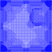
Setup 2 ($\mathcal{T}_{14,\boldsymbol{0}}$)

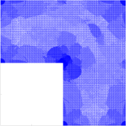
Setup 3 ($\mathcal{T}_{13,\boldsymbol{0}}$)

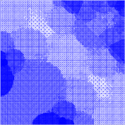
Setup 4 ($\mathcal{T}_{14,\boldsymbol{0}}$)

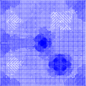
Figure 1. Adaptively refined meshes associated with the zero index at an intermediate step of Algorithm 6 for all four setups.

Figure 2. Decay of the error estimates $\mu_{\ell}\sqrt{\mu_{\ell}^{2}+\zeta_{\ell}^{2}}$ and the reference errors $\lvert\boldsymbol{g}(\boldsymbol{u}_{\mathrm{ref}})-\boldsymbol{g}(\boldsymbol{u}_{\ell})\rvert$ at each iteration of the goal-oriented adaptive algorithm for all four setups.

In Figure 2, for all setups, we plot the error estimates $\mu_{\ell}\sqrt{\mu_{\ell}^{2}+\zeta_{\ell}^{2}}$ (in red) and the reference errors $\lvert\boldsymbol{g}(\boldsymbol{u}_{\mathrm{ref}})-\boldsymbol{g}(\boldsymbol{u}_{\ell})\rvert$ (in blue) against the number of DOFs at each iteration of the goal-oriented adaptive algorithm. We observe that, for all setups, the goal-oriented adaptive algorithm drives the error estimate to zero, thus confirming the result of Theorem 7. Furthermore, we see that in each setup, the error estimate provides an upper bound for the reference error, and both quantities converge to zero with the same rate. Finally, all plots in Figure 2 show that the decay of both the error estimates and the reference errors with respect to the number of DOFs is of order $N_{\ell}^{-1}$, i.e., the best possible decay rate achievable by conforming first-order finite elements. Although the rate optimality property of Algorithm 6 for nonlinear goal functionals is not currently covered by our theoretical analysis, the results presented in Figure 2 seem to suggest that this property does hold at least for certain types of nonlinear functionals; see [BIP21] for first results in the parameter-free setting for the case of a quadratic goal functional.

6. Concluding remarks

The design of provably efficient solution strategies for high-dimensional parametric PDEs is important for reliable uncertainty quantification. Adaptive algorithms are indispensable in this context, as they provide computationally cost-effective mechanisms for generating accurate approximations and accelerating convergence. In this paper, we have designed a provably convergent goal-oriented SGFEM-based adaptive algorithm for accurate approximation of quantities of interest—linear or nonlinear functionals of solutions to elliptic PDEs with inputs depending on infinitely many parameters. Our theoretical results and algorithmic developments are valid for spatial domains in $\mathbb{R}^{2}$ and $\mathbb{R}^{3}$. Our numerical results (for two-dimensional spatial domains) show that employing the multilevel SGFEM for approximating the primal and dual solutions leads to optimal convergence rates in approximating quantities of interest. In the case of bounded linear goal functionals and for spatial domains in $\mathbb{R}^{2}$, the rate optimality property can be proved under an appropriate saturation assumption (see [BPR23]). The extension of this result to nonlinear goal functionals and three-dimensional domains is non-trivial and will be the subject of future research.

Appendix A Proof of Lemma 12

The proof is split into two steps.

Step 1. Let $\varepsilon>0$. For arbitrary $N\in\mathbb{N}$ we can choose $k_{0}\in\mathbb{N}$ such that

$$\sum_{n=1}^{N}|\alpha_{n}-\alpha_{n}^{(k)}|+C\sum_{n=1}^{\infty}|\beta_{n}-\beta_{n}^{(k)}|<\varepsilon\quad\text{for all }k\geq k_{0}.$$

Hence, by using the triangle inequality and the fact that $|\alpha_{n}^{(k)}|\leq C\,|\beta_{n}^{(k)}|$ we find that

$$\sum_{n=1}^{N}|\alpha_{n}| \leq\sum_{n=1}^{N}|\alpha_{n}^{(k)}|+\sum_{n=1}^{N}|\alpha_{n}-\alpha_{n}^{(k)}|\leq C\sum_{n=1}^{N}|\beta_{n}^{(k)}|+\sum_{n=1}^{N}|\alpha_{n}-\alpha_{n}^{(k)}|$$

$$\leq C\sum_{n=1}^{N}|\beta_{n}|+C\sum_{n=1}^{N}|\beta_{n}-\beta_{n}^{(k)}|+\sum_{n=1}^{N}|\alpha_{n}-\alpha_{n}^{(k)}|<C\sum_{n=1}^{\infty}|\beta_{n}|+\varepsilon$$

for any $\varepsilon>0$ and for arbitrary $N\in\mathbb{N}$. Therefore, $\sum_{n=1}^{\infty}|\alpha_{n}|\leq C\,\sum_{n=1}^{\infty}|\beta_{n}|<\infty.$

Step 2. Let $\varepsilon\,{>}\,0$. Since $\sum_{n=1}^{\infty}|\alpha_{n}|+C\sum_{n=1}^{\infty}|\beta_{n}|<\infty$, we can choose $n_{0}\in\mathbb{N}$ such that

$$\sum_{n=n_{0}}^{\infty}|\alpha_{n}|+C\sum_{n=n_{0}}^{\infty}|\beta_{n}|<\varepsilon.$$

Due to the assumed convergence, we can choose $k_{0}\in\mathbb{N}$ such that

$$\sum_{n=1}^{n_{0}-1}|\alpha_{n}-\alpha_{n}^{(k)}|+C\sum_{n=1}^{\infty}|\beta_{n}-\beta_{n}^{(k)}|<\varepsilon\quad\text{for all }k\geq k_{0}.$$

Then, for all $k\geq k_{0}$, the triangle inequality yields that

$$\sum_{n=1}^{\infty}|\alpha_{n}-\alpha_{n}^{(k)}| \leq\sum_{n=1}^{n_{0}-1}|\alpha_{n}-\alpha_{n}^{(k)}|+\sum_{n=n_{0}}^{\infty}|\alpha_{n}|+\sum_{n=n_{0}}^{\infty}|\alpha_{n}^{(k)}|$$

$$\leq\sum_{n=1}^{n_{0}-1}|\alpha_{n}-\alpha_{n}^{(k)}|+\sum_{n=n_{0}}^{\infty}|\alpha_{n}|+C\sum_{n=n_{0}}^{\infty}|\beta_{n}^{(k)}|$$

$$\leq\sum_{n=1}^{n_{0}-1}|\alpha_{n}-\alpha_{n}^{(k)}|+\sum_{n=n_{0}}^{\infty}|\alpha_{n}|+C\sum_{n=n_{0}}^{\infty}|\beta_{n}|+C\sum_{n=n_{0}}^{\infty}|\beta_{n}-\beta_{n}^{(k)}|<2\varepsilon.$$

This concludes the proof.

References

- [AO10] R. C. Almeida and J. T. Oden. Solution verification, goal-oriented adaptive methods for stochastic advection–diffusion problems. Comput. Methods Appl. Mech. Engrg., 199(37-40):2472–2486, 2010.
- [BDW11] T. Butler, C. Dawson, and T. Wildey. A posteriori error analysis of stochastic differential equations using polynomial chaos expansions. SIAM J. Sci. Comput., 33(3):1267–1291, 2011.
- [BIP21] R. Becker, M. Innerberger, and D. Praetorius. Optimal convergence rates for goal-oriented FEM with quadratic goal functional. Comp. Meth. Appl. Math., 21:267–288, 2021.
- [BPR21] A. Bespalov, D. Praetorius, and M. Ruggeri. Two-level a posteriori error estimation for adaptive multilevel stochastic Galerkin FEM. SIAM/ASA J. Uncertain. Quantif., 9(3):1184–1216, 2021.
- [BPR22] A. Bespalov, D. Praetorius, and M. Ruggeri. Convergence and rate optimality of adaptive multilevel stochastic Galerkin FEM. IMA J. Numer. Anal., 42(3):2190–2213, 2022.
- [BPR23] A. Bespalov, D. Praetorius, and M. Ruggeri. Optimal convergence rates for goal-oriented adaptive multilevel stochastic Galerkin FEM. In preparation, 2023.
- [BPRR19a] A. Bespalov, D. Praetorius, L. Rocchi, and M. Ruggeri. Convergence of adaptive stochastic Galerkin FEM. SIAM J. Numer. Anal., 57(5):2359–2382, 2019.
- [BPRR19b] A. Bespalov, D. Praetorius, L. Rocchi, and M. Ruggeri. Goal-oriented error estimation and adaptivity for elliptic PDEs with parametric or uncertain inputs. Comput. Methods Appl. Mech. Engrg., 345:951–982, 2019.
- [BPW15] C. Bryant, S. Prudhomme, and T. Wildey. Error decomposition and adaptivity for response surface approximations from PDEs with parametric uncertainty. SIAM/ASA J. Uncertain. Quantif., 3(1):1020–1045, 2015.
- [BR18] A. Bespalov and L. Rocchi. Efficient adaptive algorithms for elliptic PDEs with random data. SIAM/ASA J. Uncertain. Quantif., 6(1):243–272, 2018.
- [BR22] A. Bespalov and L. Rocchi. Stochastic T-IFISS, January 2022. Available online at https://web.mat.bham.ac.uk/A.Bespalov/software/index.html#stoch_tifiss.
- [BRS21] A. Bespalov, L. Rocchi, and D. Silvester. T-IFISS: a toolbox for adaptive FEM computation. Comput. Math. Appl., 81:373–390, 2021.
- [BS16] A. Bespalov and D. Silvester. Efficient adaptive stochastic Galerkin methods for parametric operator equations. SIAM J. Sci. Comput., 38(4):A2118–A2140, 2016.
- [BV84] I. Babuška and M. Vogelius. Feedback and adaptive finite element solution of one-dimensional boundary value problems. Numer. Math., 44:75–102, 1984.
- [CD15] A. Cohen and R. DeVore. Approximation of high-dimensional parametric PDEs. Acta Numer., 24:1–159, 2015.
- [CPB19] A. J. Crowder, C. E. Powell, and A. Bespalov. Efficient adaptive multilevel stochastic Galerkin approximation using implicit a posteriori error estimation. SIAM J. Sci. Comput., 41(3):A1681–A1705, 2019.
- [CST13] J. Charrier, R. Scheichl, and A. L. Teckentrup. Finite element error analysis of elliptic PDEs with random coefficients and its application to multilevel Monte Carlo methods. SIAM J. Numer. Anal., 51(1):322–352, 2013.
- [Dör96] W. Dörfler. A convergent adaptive algorithm for Poisson’s equation. SIAM J. Numer. Anal., 33(3):1106–1124, 1996.
- [EGP20] C. Erath, G. Gantner, and D. Praetorius. Optimal convergence behavior of adaptive FEM driven by simple -type error estimators. Comput. Math. Appl., 79(3):623–642, 2020.
- [EGSZ14] M. Eigel, C. J. Gittelson, C. Schwab, and E. Zander. Adaptive stochastic Galerkin FEM. Comput. Methods Appl. Mech. Engrg., 270:247–269, 2014.
- [EGSZ15] M. Eigel, C. J. Gittelson, C. Schwab, and E. Zander. A convergent adaptive stochastic Galerkin finite element method with quasi-optimal spatial meshes. ESAIM Math. Model. Numer. Anal., 49(5):1367–1398, 2015.
- [EM16] M. Eigel and C. Merdon. Local equilibration error estimators for guaranteed error control in adaptive stochastic higher-order Galerkin finite element methods. SIAM/ASA J. Uncertain. Quantif., 4(1):1372–1397, 2016.
- [EMN16] M. Eigel, C. Merdon, and J. Neumann. An adaptive multilevel Monte Carlo method with stochastic bounds for quantities of interest with uncertain data. SIAM/ASA J. Uncertain. Quantif., 4(1):1219–1245, 2016.
- [GS02] M. B. Giles and E. Süli. Adjoint methods for PDEs: a posteriori error analysis and postprocessing by duality. Acta Numer., 11:145–236, 2002.
- [GWZ14] M. D. Gunzburger, C. G. Webster, and G. Zhang. Stochastic finite element methods for partial differential equations with random input data. Acta Numer., 23:521–650, 5 2014.
- [MLM07] L. Mathelin and O. Le Maître. Dual-based a posteriori error estimate for stochastic finite element methods. Comm. App. Math. Com. Sc., 2(1):83–115, 2007.
- [MS09] M. S. Mommer and R. Stevenson. A goal-oriented adaptive finite element method with convergence rates. SIAM J. Numer. Anal., 47:861–886, 2009.
- [MSV08] P. Morin, K. G. Siebert, and A. Veeser. A basic convergence result for conforming adaptive finite elements. Math. Models Methods Appl. Sci., 18(5):707–737, 2008.
- [SG11] C. Schwab and C. J. Gittelson. Sparse tensor discretizations of high-dimensional parametric and stochastic PDEs. Acta Numer., 20:291–467, 2011.
- [Ste08] R. Stevenson. The completion of locally refined simplicial partitions created by bisection. Math. Comp., 77(261):227–241, 2008.
- [TSGU13] A. L. Teckentrup, R. Scheichl, M. B. Giles, and E. Ullmann. Further analysis of multilevel Monte Carlo methods for elliptic PDEs with random coefficients. Numer. Math., 125(3):569–600, 2013.