Thermodynamic properties, thermal image and phase transition of Einstein-Gauss-Bonnet black hole coupled with nonlinear electrodynamics

Abstract

We obtain an exact solution of $AdS$ black hole solution in Einstein-Gauss-Bonnet (EGB) gravity coupled with nonlinear electrodynamics. It interpolates with the $AdS$ regular black hole and $AdS$ EGB black hole in the absence of the Gauss-Bonnet coupling constant and both magnetic monopole charge and deviation parameter, respectively. Based on horizon thermodynamics, we study the thermodynamic properties of the obtained solution (e.g. mass, temperature, entropy, heat capacity and free energy). The Hawking temperature of the nonsingular black hole gets the maximum value at the point where specific heat diverges and the second-order phase transition occurs at the same point. We find that the smaller nonsingular black holes are stable due to positive heat capacity and negative free energy. We explicitly trace the relations between the black hole shadow and the critical behavior of charged EGB $AdS$ regular black hole in the extended phase space.

I Overview and motivation

Black holes, one of the most fascinating objects of nature, were predicted by Einstein’s gravity in general relativity (GR). This is because the geometric properties of black holes are described by elegant mathematical equations. The recent (astrophysical) observations and experiments associated with gravitational waves 1 ; 2 and (supermassive) black hole shadows 3 can guide us to test the different gravity models. Due to the limitations of Einstein’s gravity, modifications to Einstein’s gravity have been studied widely in the cosmological context. In this connection, the modifications in the form of higher orders of the Riemann curvature (and of its contractions) had been discussed for the sake of answer to the problem of the dark energy dominance in the evolution of our universe as well as the hierarchy problem. Lee-Wick gravity theories, on the other hand, are another example of modified gravity that removes the conflict between unitarity and renormalizability in quantum gravity l ; l1 ; sd .

In general, gravity theories with higher derivative curvature terms had consistency issues due to negative norm states (ghost) in their spectra at the quantum level. Lovelock gravity is one of the higher derivative gravity theories that maintain second-order equations of motion for the metric and makes the theory ghost-free lav . Gauss-Bonnet (GB) or Einstein-Gauss-Bonnet (EGB) gravity is particular Lovelock gravity that gets relevance in higher dimensions 4 . Interestingly, higher orders of the Riemann curvature corrections appear naturally in the low-energy limit of string theory 5 . This gave rise to considerable interest in EGB gravity theories (especially, the black-hole solutions of these theories) 6 ; 7 . The GB term is not dynamical in $4d$ due to total derivative. It becomes dynamical in $4d$ only when GB term must be coupled to a matter field otherwise dimension should be greater than four. Quite interestingly, by re-scaling the GB coupling constant $\alpha\to\alpha/d-4$, the EGB the black hole solutions in $4d$ have been studied gla where the GB term contributes to the (local) dynamics gla . The consistency of field-equation is rather questioned me . The limit $d\to 4$ costs us by either partial breaking of the diffeomorphism or leading to additional degrees of freedom.

In Refs. gl1 ; gl2 , a consistent EGB gravity in $4d$ has been proposed that admits spatial covariance only but not the temporal covariance. Recently, black hole solution and their thermal properties have been studied for 4D $AdS$ EGB gravity coupled with Yang-Mills field Singh:2021xbk . Moreover, a black hole solution along with its thermodynamics for $4D$ EGB gravity fran , $4D$ EGB massive gravity is presented Upadhyay:2022axg , $4D$ EGB wormhole solutions Godani:2022jwz ; Jusufi:2020yus , and $4D$ EGB quark star Tangphati:2021tcy ; Pretel:2021czp ; Tangphati:2021wng ; Panotopoulos:2022dbu .

From the perspective of GR and its extensions, nonlinear electrodynamics is one of the most crucial material sources of gravity as it leads to many interesting geometries, in particular, regular black holes. The nonlinear electrodynamics is an extension of the Maxwell electrodynamics which came into the picture due to Born and Infeld (BI) in removing the central singularity of a point charge be . A generalized BI action appears naturally in superstrings scenario 8 ; 9 induces interest in nonlinear electrodynamics. Black holes with nonlinear electrodynamics as a matter source are of great importance in astrophysical observations and, therefore, studied extensively 10 ; 11 ; nnn ; ab ; abg11 ; abg ; 12 ; 13 ; sabir ; dvs1 ; kumar1 ; dvs2 . However, the first regular black hole was proposed by Bardeen 14 . In the context of nonlinear electrodynamics, it is shown that a regular black hole only describes the formation of a black hole from an initial vacuum region. The preference for nonlinear electrodynamics over Maxwell’s theory is only because, along with the conformal breaking, the infinite electric field and self-energy also appear at the position of a point charge.

After Bekenstein and Hawking’s proposal of black hole entropy 16 and black hole radiation 17 , black holes are being considered as a thermal system. Bekenstein stated that the addition of black hole entropy and the the entropy of matter is a non-decreasing function of time. The generalized second law of thermodynamics suggests that black holes and self-gravitating systems comprise a larger thermodynamic space. This leads to the possibility of phase transitions between black holes and self-gravitating systems. Understanding such phase transitions is itself important. Such analysis may provide significantly insights to quantum theories of gravity 15 .

The plan of the paper is as follows. In Sec. II, we get an exact black hole solution for the EGB gravity coupled with nonlinear electrodynamics and negative cosmological constant. In Sec. III, we provide a thermal description of the obtained solution by computing mass, temperature and entropy. Within section, we also discuss the local and global stability of the system. In Sec. IV, we study the $P-v$ criticality and phase diagram of the resulting black hole solution. In Sec. V, we outline the relation between phase transition and Shadow radius. Within section, we discuss the effects of various parameter on black hole shadow. The discussion of results is reported in the last section.

II $4D$ regular EGB Black hole solution

The action of EGB gravity coupled with nonlinear electrodynamics and negative cosmological constant can be written as

$$S = \frac{1}{2}\int d^{d}x\sqrt{-g}\left[{R}-2\Lambda+\frac{\alpha}{D-4}{\cal L_{GB}}-2{L}(F)\right],$$ (1)

where $\alpha$ represents the dimensionless GB coupling constant, and ${R}$ denotes $D$-dimensional curvature scalar, the GB Lagrangian density is given by $\mathcal{L_{GB}}:=R_{abcd}R^{abcd}-4R_{ab}R^{ab}+R^{2}$. Here, ${L}(F)$ corresponds to matter Lagrangian which depends on $F=\frac{1}{4}F_{ab}F^{ab}$.
Variation the action (1) with respect to $g_{ab}$ and the potential $A_{a}$, we obtained the following equations of motion:

$$R_{ab}-\frac{1}{2}\tilde{g}_{ab}R+\Lambda g_{ab}+\frac{\alpha}{d-4}H_{ab}=T_{ab}\equiv 2\left[\frac{\partial{{L(F)}}}{\partial F}F_{ac}F_{\ b}^{c}-\tilde{g}_{ab}{{L(F)}}\right],$$ (2)

$$\nabla_{a}\left(\frac{\partial{{L(F)}}}{\partial F}F^{ab}\right)=0\qquad\text{and}\qquad\nabla_{a}(*F^{ab})=0,$$ (3)

where GB tensor is expressed as

$$H_{ab}=-\frac{1}{2}\left[8R^{cd}R_{acbd}-4R_{a}^{\ cde}R_{bcde}-4RR_{ab}+8R_{ac}R_{\ b}^{c}+g_{ab}\left(R_{cdef}R^{cdef}-4R_{cd}R^{cd}+R^{2}\right)\right].$$ (4)

Here, we note that the GB invariant in $d=4$ does not contribute to the field equations. So, let us briefly explain the idea of how GB term contributes to the dynamics of gravitational field by re-scaling the GB coupling constant to $\alpha/(d-4)$. For maximally symmetric solution, Riemann tensor is given by gla $R^{ab}_{\ \ cd}=(\delta^{a}_{\ c}\delta^{b}_{\ d}-\delta^{a}_{\ d}\delta^{b}_{\ c})\Lambda_{eff}/(d-1)$, where $\Lambda_{eff}$ is an effective cosmological constant. To estimate Gauss-Bonnet contribution, one calculates gla

$$\frac{g_{bc}}{\sqrt{-g}}\frac{{\cal L_{GB}}}{\delta g_{ac}}=\frac{(d-2)(d-3)(d-4)}{2(d-1)}\Lambda_{eff}\delta^{a}_{b}.$$ (5)

Here, the appeared vanishing factor $(d-4)$ due to Gauss-Bonnet term in $4D$ gets canceled by the divergent factor $1/(d-4)$ coming from the re-scaling GB coupling constant $\alpha/(d-4)$.

Here, we are interested in a particular form of the nonlinear electrodynamics Lagrangian $L(F)$ which admits the freedom of the duality rotations as discussed in Refs. nnn ; ab ; abg11 . This is given by

$${{L(F)}}=\frac{Fe^{-s(2g^{2}F)^{1/4}}}{(1+\sqrt{2g^{2}F})^{3/2}}\left(1+\frac{3}{s}\frac{(2g^{2}F)^{1/4}}{(1+\sqrt{2g^{2}F)}}\right),$$ (6)

where $s=|g|/2M$ with the free parameters $g$ and $M$ associated with magnetic charge and mass, respectively. For weak fields, this nonlinear electrodynamics correspondence to Maxwell theory.

To obtain a static spherically symmetric black hole solution in $4D$, we consider the following line element:

$$ds^{2}=-f(r)dt^{2}+\frac{1}{f(r)}dr^{2}+r^{2}d\Omega_{2}^{2},$$ (7)

where $f(r)$ is the metric and $d\Omega_{2}^{2}=d\theta^{2}+\sin^{2}\theta d\phi^{2}$ is the metric of a $2$-dimensional sphere.

To determine the metric function, we consider the following magnetic choice for the Maxwell’s field-strength tensor $F_{ab}$ abg ; Singh:2022xgi

$$F_{ab}=2\delta^{\theta}_{[a}\delta^{\phi}_{b]}Y(r,\theta).$$ (8)

Here, we must stress that there exists spherically symmetric solutions with a globally regular metric for gravity coupled to nonlinear electrodynamics with the Lagrangian $L(F)$, possessing a correct weak field limit, for the magnetic case only Bronnikov:2017tnz ; Bronnikov:2000vy . However, the electric analogs of magnetic solutions can be found with different Lagrangian (using a Legendre transformation in Hamiltonian formalism) in different ranges of the radial coordinate Bronnikov:2000vy .

With ansatz (8), the integration of equation (3) give rise to

$$F_{ab}=2\delta^{\theta}_{[a}\delta^{\phi}_{b]}g\sin\theta.$$ (9)

Here, $g$ is constant (independent of $r$) is confirmed by using exterior derivative of differential 2-form (8). Now, the field-strength tensor and, therefore, matter Lagrangian can be simplified to

$$F_{\theta\phi}=g\sin\theta,\qquad F=\frac{1}{2}\frac{g^{2}}{r^{4}},\qquad\text{and}\qquad{L(F)}=\frac{g^{2}}{2r^{2}}\frac{e^{-sg/r}}{(r^{2}+g^{2})^{3/2}}\left[1+\frac{g}{s}\frac{r}{(r^{2}+g^{2})}\right].$$ (10)

The non-zero components of energy momentum tensor are given by

$$T^{t}_{t}=T^{r}_{r} = \frac{g^{2}}{2r^{2}}\frac{e^{-sg/r}}{(r^{2}+g^{2})^{3/2}}\left[1+\frac{g}{s}\frac{r}{(r^{2}+g^{2})}\right],$$ (11)

$$T^{\theta}_{\theta}=T^{\phi}_{\phi} = \frac{g^{2}}{4r^{2}}\frac{e^{-sg/r}}{(r^{2}+g^{2})^{3/2}}\left[1+\frac{g}{s}\frac{r}{(r^{2}+g^{2})}-\frac{g(3g^{2}+8r^{2})}{sr}\right.$$ (12)

$$- \left.\frac{(3g^{2}+7r^{4})}{r^{2}(r^{2}+g^{2})^{5/2}}+\frac{gs}{r^{3}(r^{2}+g^{2})^{3/2}}\right].$$

The $(r,r)$ components of Eq. (2) in the limit $d\to 4$ gives

$$r^{5}-2r^{3}\alpha(f-1)\frac{df}{dr}+r^{4}(f-1)+r^{2}\alpha(f-1)^{2}-\Lambda r^{2}=\frac{g^{2}}{4r^{2}}\frac{e^{-sg/r}}{(r^{2}+g^{2})^{3/2}}\left[1+\frac{g}{s}\frac{r}{(r^{2}+g^{2})}\right].$$ (13)

The solution of above equation is given by

$$f_{\pm}(r)=1+\frac{r^{2}}{2\alpha}\pm\frac{r^{2}}{2\alpha}\sqrt{1+\frac{8M\alpha\,e^{-k/r}}{(r^{2}+g^{2})^{3/2}}-\frac{4\alpha}{l^{2}}},$$ (14)

where $k\,(=g^{2}/2M)$ is called as deviation parameter that measures the deviation from Schwarzschild black hole solution. For $AdS$, the cosmological constant ($\Lambda$) can be expressed in terms of length scale $l$ as $\Lambda=-3/l^{2}$. Here, $M$ is a constant of integration related to the total mass of the black hole. The obtained black hole solution (14) is characterized by the mass, deviation parameter, magnetic charge, GB coupling constant ($\alpha$) and cosmological constant. In the absence of deviation parameter, this solution (14) identifies to the following $4D$ EGB Bardeen black hole Singh:2020xju :

$$f_{\pm}(r)=1+\frac{r^{2}}{2\alpha}\pm\frac{r^{2}}{2\alpha}\sqrt{1+\frac{8M\alpha\,}{(r^{2}+g^{2})^{3/2}}-\frac{4\alpha}{l^{2}}}.$$ (15)

In the absence of magnetic charge, this solution identifies to following $4D$ EGB regular black hole Singh:2020mty :

$$f_{\pm}(r)=1+\frac{r^{2}}{2\alpha}\pm\frac{r^{2}}{2\alpha}\sqrt{1+\frac{8M\alpha\,e^{-k/r}}{r^{3}}-\frac{4\alpha}{l^{2}}}.$$ (16)

In the absence of GB coupling parameter, this identifies to solution obtained in Ref. abg

$$f(r)=1+\frac{2Mr^{2}e^{-k/r}}{(r^{2}+g^{2})^{3/2}}+\frac{r^{2}}{l^{2}}.$$ (17)

Moreover, our solution reduces to $AdS$ EGB black hole gla , Bardeen black hole, $AdS$ regular black hole tzi and $AdS$ Schwarzschild black hole in the limit of $g=k=0$ and $\alpha=0$, respectively.

The solutions (14) behaves asymptotically as

$$f_{-}=1-\frac{2Me^{-k/r}}{(r^{2}+g^{2})^{3/2}}+\frac{r^{2}}{l^{2}}+\frac{r^{2}}{2\alpha}+{{\cal O}\left(\frac{1}{r^{3}}\right)},$$ (18)

$$f_{+}=1+\frac{2Me^{-k/r}}{(r^{2}+g^{2})^{3/2}}-\frac{r^{2}}{l^{2}}+\frac{r^{2}}{2\alpha}+{{\cal O}\left(\frac{1}{r^{3}}\right)}.$$ (19)

Here, one can see that the $+$ve branch of the solutions is not physical as the positive mass term indicates graviton instabilities and, therefore, this solution will be ruled out. However, $-$ve branch of the solutions matches with the physical $4D$ $AdS$ EGB black hole solution, so we must stick with it. In the limit $r\to\infty$ ($M=0$), the EGB black hole solution (18) becomes asymptotically flat.

In the limit $k=g=0$, the solution (14) reduces to

$$f_{\pm}(r)=1+\frac{r^{2}}{2\alpha}\left(1\pm\sqrt{1+\frac{8M\alpha}{r^{3}}-\frac{4\alpha}{l^{2}}}\,\right).$$ (20)

This solution coincides with the one obtained by Glavan and Lin in Ref. gla . This even matches further with $4D$ $AdS$ Schwarzschild black hole solution in limit $\alpha\to 0$.

As we know that $f(r)=0$ determines the horizons. Since Eq. (14) is a transcendental equation and can not be solved analytically. So, to determine the horizons of the black hole, we solve it numerically and the numerical results are tabulated in the TAB. 1.

	$\alpha=0.1$					$\alpha=0.2$
$g$	$r_{+}$	$r_{-}$	$\delta$	$g$	$r_{+}$	$r_{-}$	$\delta$
0.20	1.77	0.25	1.52	0.20	1.71	0.33	1.38
0.40	1.64	0.45	1.19	0.40	1.56	0.57	0.99
0.63	1.08	1.08	0.00	0.57	1.11	1.11	0.00
	$\alpha=0.1$					$\alpha=0.2$
$k$	$r_{+}$	$r_{-}$	$\delta$	$g$	$r_{+}$	$r_{-}$	$\delta$
0.10	1.72	0.33	1.39	0.10	1.65	0.44	1.21
0.30	1.44	0.51	0.93	0.30	1.31	0.66	0.65
0.47	0.92	0.92	0.00	0.385	0.97	0.97	0.00

Table 1: Cauchy horizon ($r_{-}$) and event horizon ($r_{+}$) and their deviation $\delta=r_{+}-r_{-}$ for different values of $g$ and $k$ and fixed value of $l$ and $M$.

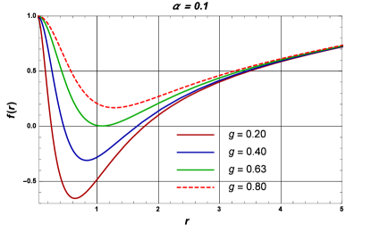
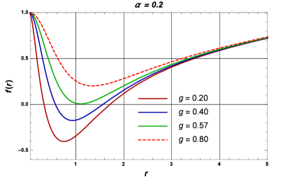
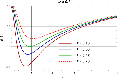
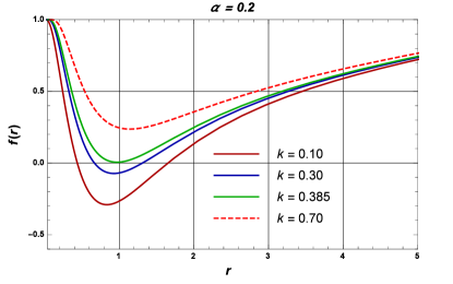
Figure 1: Metric function $f(r)$ versus horizon radius for different magnetic monopole charge $(g)$ and deviation parameter ($k$) with fixed values of GB parameter $\alpha=0.1$ and $\alpha=0.2$. Here, we set $M=1$.

In the Fig. 1, we notice how the horizon structure depends on parameters $k$ and $g$. The zeros of metric function declares that there is no horizon if $k>k_{c}$ (or $g>g_{c}$), one horizon if $k=k_{c}$ (or $g=g_{c}$), and are two horizon if $k<k_{c}=0.47$ (or $g<g_{c}=0.60$). It is worthwhile to mention that the size of horizon increases with decreasing magnetic charge $(g)$ and deviation parameter $(k)$. The same effect also appears for the GB coupling. The TABLE 1 reflects the values of event (outer) horizon and Cauchy (inner) horizon.

In order to study the nature of singularities of $AdS$ black hole (14), curvature invariants of Ricci square ($R_{\mu\nu}R^{\mu\nu}$) and Kretshmann scalars ($R_{\mu\nu\lambda\sigma}R^{\mu\nu\lambda\sigma}$) are important. The behaviors of the scalar invariants are given by

$$R=f^{\prime\prime}(r)+\frac{6f^{\prime}(r)}{r}-\frac{6(1-f(r))}{r^{2}},$$ (21)

$$R^{\mu\nu}R_{\mu\nu}=\frac{1}{2}{{f^{\prime\prime}(r)^{2}}}+\frac{15}{2}{\left({\frac{{f^{\prime}(r)}}{{r}}}\right)^{2}}+\frac{2}{r}f^{\prime\prime}(r)f(r)+\frac{12}{r^{4}}f(r)^{2}-\frac{24}{r^{4}}f(r)$$

$$\qquad\qquad-\frac{24}{r^{4}}(rf^{\prime}(r)+1)+\frac{24}{r^{3}}f(r)f^{\prime}(r),$$ (22)

$$R^{\mu\nu\lambda\rho}R_{\mu\nu\lambda\rho}={{f^{\prime\prime}(r)^{2}}}+6{\left({\frac{{f^{\prime}(r)}}{{r}}}\right)^{2}}+12{\left({\frac{{f(r)-1}}{{{r^{2}}}}}\right)^{2}}.$$ (23)

These invariants are smooth in $r\to 0$ limit and, therefore, signify regular space-time.

III Thermodynamics

In this section, we investigate the thermal properties of $4D$ $AdS$ EGB regular black hole. In this connection, we discuss, particularly, mass, temperature, entropy, specific heat, and Gibbs free energy at the black hole horizon. The mass of the black hole can be estimated from the metric function (14) on the horizon as

$$M=\left(g^{2}+r_{+}^{2}\right)^{3/2}e^{k/r_{+}}\Big{[}\frac{(\alpha+r_{+}^{2})}{2r_{+}^{4}}+\frac{1}{2l^{2}}\Big{]}.$$ (24)

This expression represents the mass of regular black hole in $4D$ EGB gravity (24). From the above expression, it is clear that, for $k=0$ it reduces to the mass of the $AdS$ EGB Bardeen black hole Singh:2020xju , for $g=0$ it reduces to $AdS$ EGB regular black hole Singh:2020mty and for both $k=0,g=0$ it reduces to $4D$ EGB black hole gla . For vanishing $\alpha$ and $k$, the above expressing reduces to the mass of Bardeen black hole tzi and for vanishing $\alpha$ and $g=0$ it reduces to the mass of $AdS$ regular black hole. Finally, it reduces to mass of the $AdS$ Schwarzschild black hole for vanishing all three parameters: $g$, $\alpha$ and $k$.

The standard formula to calculate Hawking temperature is given by

$$T_{+}=\frac{1}{2\pi}{\sqrt{-\frac{1}{2}\nabla_{\mu}\xi_{\nu}\nabla^{\mu}\xi^{\nu}}}=\frac{1}{4\pi}f^{\prime}(r_{+}).$$ (25)

In our case, this leads to

$$T_{+} = \frac{1}{4\pi r_{+}}\bigg{(}\frac{3r_{+}^{7}+l^{2}r_{+}^{2}(\alpha+r_{+}^{2})(9r-2k)-k(g^{2}+r_{+}^{2})(\alpha l^{2}+l^{2}r_{+}^{2}+r_{+}^{4})}{l^{2}r_{+}(g^{2}+r_{+}^{2})(r_{+}^{2}+2\alpha)}\bigg{)}.$$ (26)

From the expression of Hawking temperature it is clear that when $k=0$ it identifies to the Hawking temperature of the $AdS$ EGB Bardeen black hole Singh:2020xju and and to the $AdS$ EGB regular black hole Singh:2020mty for $g=0$. In the limit of $\alpha=0$, the Hawking temperature reduces to

$$T_{+} = \frac{1}{4\pi r_{+}}\bigg{(}\frac{3r_{+}^{7}+l^{2}r_{+}^{4}(9r-2k)-k(g^{2}+r_{+}^{2})(l^{2}r_{+}^{2}+r_{+}^{4})}{l^{2}r^{3}_{+}(g^{2}+r_{+}^{2})(r_{+}^{2}+2)}\bigg{)}.$$ (27)

In order to analyze the behavior of temperature for the various values of magnetic charge $g$ and the deviation parameter $k$, we plot Fig. 2.

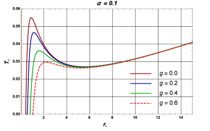
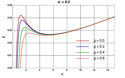
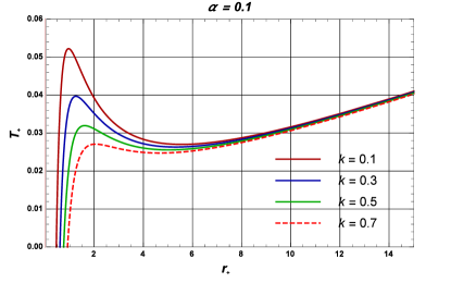
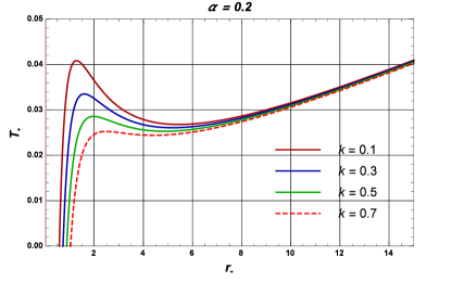
Figure 2: Temperature versus horizon radius for different valued of magnetic monopole charge $(g)$ and deviation parameter ($k$) with fixed values of GB parameter $\alpha=0.1$ and $\alpha=0.2$. Here, we set $l=10$.

Here, we see that the temperature first grows to a maximum value of $T_{+}^{max}$ and then it drops to a minimum value, and then it starts growing again.

The maximum values of temperature for different values of parameters are tabulated in TABLES 2 and 3.

	$\alpha=0.1$,  $k=0.1$			$\alpha=0.2$,  $k=0.1$
$g$	$r$	$T_{+}^{max}$	$g$	$r$	$T_{+}^{max}$
0.00	0.89	0.055	0.00	1.22	0.042
0.20	1.12	0.047	0.20	1.42	0.038
0.40	1.59	0.036	0.40	1.86	0.032

Table 2: The values of maximum Hawking temperature for the $4D$ AdS EGB regular black hole with different values of parameters and fixed value of $l=10$.

	$\alpha=0.1$,  $g=0.1$			$\alpha=0.2$,  $g=0.1$
$k$	$r$	$T_{+}^{max}$	$k$	$r$	$T_{+}^{max}$
0.10	0.95	0.052	0.10	1.27	0.040
0.30	1.25	0.039	0.30	1.62	0.035
0.50	1.60	0.032	0.50	2.00	0.029

Table 3: The values of maximum Hawking temperature for the $4D$ AdS EGB regular black hole with different values of parameters and fixed value of $l=10$.

From these TABLES, we see that the values of maximum temperature decrease with an increase in the values of $g$ and $k$. The maximum temperature diverges when the horizon radius shrinks to zero. Fig. 2 also suggests that the Hawking temperature vanishes when the two horizons (Cauchy and event) merge.

The thermodynamical quantities must follow the first law of thermodynamics

$$dM=T_{+}dS_{+}.$$ (28)

Since we have explicit expressions of mass and Hawking temperature, then the first law gives the value of entropy as

$$S_{+}=\pi r_{+}^{2}+4\alpha\log[r_{+}].$$ (29)

Now, we are interested in the stability of this black hole. We are aware that local stability is decided by the signature of heat capacity. The positive indicates that the system is stable and the negative indicates the unstable one sabir ; dvs1 ; kumar1 . However, the global stability can be studied from the Gibbs free energy.

Now, we first calculate from the given formula

$$C_{+}=\frac{\partial M}{\partial T_{+}}=\bigg{(}\frac{\partial M}{\partial r_{+}}\bigg{)}\bigg{(}\frac{\partial r_{+}}{\partial T_{+}}\bigg{)}.$$ (30)

This gives

$$C_{+}=-\frac{2\pi\left(g^{2}+r_{+}^{2}\right)^{5/2}e^{k/r_{+}}\left(2\alpha+r_{+}^{2}\right)^{2}\bigg{(}-k\left(g^{2}+r_{+}^{2}\right)\left(l^{2}\left(\alpha+r_{+}^{2}\right)+r_{+}^{4}\right)+\mathcal{X}\bigg{)}}{r_{+}^{3}\bigg{(}2l^{2}g^{4}r_{+}\left(2\alpha+r_{+}^{2}\right)^{2}+2k\left(g^{2}+r_{+}^{2}\right)^{2}\mathcal{W}+\mathcal{Y}+\mathcal{Z}\bigg{)}},$$ (31)

where

$$\mathcal{W}=l^{2}\left(2\alpha^{2}+r_{+}^{4}+2\alpha r_{+}^{2}\right)-2\alpha r_{+}^{4},$$ (32)

$$\mathcal{X}=-2g^{2}l^{2}r_{+}\left(2\alpha+r_{+}^{2}\right)+l^{2}r_{+}^{3}\left(r_{+}^{2}-\alpha\right)+3r_{+}^{7},$$ (33)

$$\mathcal{Y}=g^{2}r_{+}^{2}\left(l^{2}\left(7r_{+}^{5}+31\alpha r_{+}^{3}+22\alpha^{2}r_{+}\right)+9r_{+}^{7}+30\alpha r_{+}^{5}\right),$$ (34)

$$\mathcal{Z}=r_{+}^{4}\left(l^{2}\left(-r_{+}^{5}+5\alpha r_{+}^{3}+2\alpha^{2}r_{+}\right)+3\left(r_{+}^{7}+6\alpha r_{+}^{5}\right)\right).$$ (35)

From the Eq. (31), it is evident that the heat capacity depends on all the parameters $g$, $k$, $\alpha$, and $\Lambda$. For $k=0$, it coincides with the mass of the heat capacity of $AdS$ EGB Bardeen black hole Singh:2020xju . The heat capacity in absence of the GB parameter reduces to

$$C_{+}=-\frac{2\pi\left(g^{2}+r_{+}^{2}\right)^{5/2}e^{k/r_{+}}r_{+}^{4}\bigg{(}-k\left(g^{2}+r_{+}^{2}\right)\left(l^{2}\left(r_{+}^{2}\right)+r_{+}^{4}\right)+\mathcal{X}\bigg{)}}{r_{+}^{3}\bigg{(}2l^{2}g^{4}r_{+}\left(r_{+}^{2}\right)^{2}+2k\left(g^{2}+r_{+}^{2}\right)^{2}\mathcal{W}+\mathcal{Y}+\mathcal{Z}\bigg{)}},$$ (36)

with

$$\mathcal{W}=l^{2}r_{+}^{4},\qquad\qquad\mathcal{X}=\left(-2g^{2}l^{2}r_{+}^{3}+l^{2}r_{+}^{5}+3r_{+}^{7}\right),$$ (37)

$$\mathcal{Y}=g^{2}r_{+}^{2}\left(7r_{+}^{5}l^{2}+9r_{+}^{7}\right),\qquad\text{and}\qquad\mathcal{Z}=r_{+}^{4}\left(-l^{2}r_{+}^{5}+3r_{+}^{7}\right).$$ (38)

Here, we observe that the expression of heat capacity we obtain is the most general one. The various limiting case can be studied just by switching various parameters off.

Now, the stability can be checked when one observes the plots of heat capacity for fixing the parameters as depicted in FIG. 3.

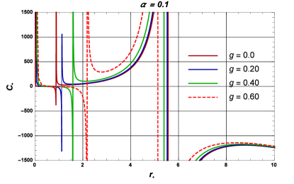
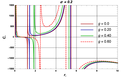
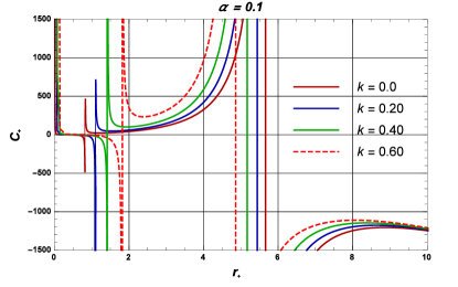
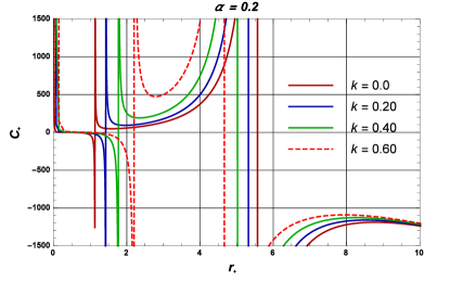
Figure 3: The heat capacity $C_{+}$ versus horizon radius with the different values of $g$ and $k$ for two fixed value of GB parameter $\alpha=0.1$ and $\alpha=0.2$.

The heat capacity is showing discontinuity at a particular point (say critical radius $r_{+}=r_{C}$) which signifies a second-order phase transition. Remarkably, at this point of critical radius, the temperature attains the maximum value $T_{+}^{max}$. Hence, a phase transition occurs in-between stable and unstable phases when the black hole gets bigger.

Now we turn to the global stability of the black hole, which is characterized by Gibbs free energy. The Gibbs free energy can be estimated by standard definition $F_{+}=M-T_{+}S_{+}$, as follows

$$F_{+} = \frac{\left(g^{2}+r_{+}^{2}\right)^{3/2}\left(\alpha l^{2}+l^{2}r_{+}^{2}+r_{+}^{4}\right)e^{k/r_{+}}}{2l^{2}r_{+}^{4}}$$ (39)

$$+ \frac{k(g^{2}+r_{+}^{2})(\alpha l^{2}+l^{2}r_{+}^{2}+r_{+}^{4})-3r_{+}^{7}-l^{2}r_{+}^{2}(\alpha+r_{+}^{2})(9r_{+}-2k)}{4l^{2}(g^{2}+r_{+}^{2})(r_{+}^{2}+2\alpha)}.$$

Since, global stability of the black hole is confirmed by condition $F_{+}\leq 0$. Now, to analyze the behavior of this expression, we plot FIG. 4.

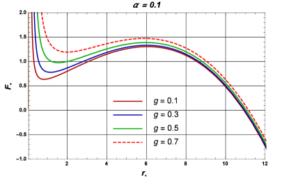
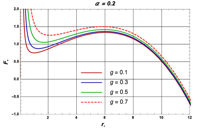
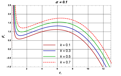
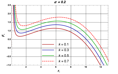
Figure 4: Gibbs free energy versus horizon radius for different values of $g$ and $k$ with fixed values of GB parameter $\alpha=0.1$ and $\alpha=0.2$.

Here, we observe that there exists a local minimum ($r_{min}$) and maximum ($r_{max}$) which are in agreement with the extremal points of Hawking temperature. At this point free energy change nature. After this point ${r_{min}}$, the free energy increases with horizon radius $r$ and attains the maximum value at $r_{max}$. After this point, the free energy decreases with the horizon radius.

IV $P-v$ Criticality and Phase Diagrams

Now, we plan to explore the critical behavior of the present black hole solution in an extended phase space, by considering $\Lambda$ as the thermodynamic pressure. The cosmological constant appears in the pressure as $P=-\frac{\Lambda}{8\pi}=\frac{3}{8\pi l^{2}}$. Plugging the value of $l$ from Eq. (26), the form of pressure becomes

$$P=\frac{3T(r_{+}^{6}+2r_{+}^{4}\alpha+g^{2}r_{+}^{2}(r_{+}^{2}+2\alpha))}{2r_{+}^{4}(g^{2}k+(k-3r_{+})r_{+}^{2})}+\frac{3(r_{+}^{5}-r_{+}^{2}+\alpha+(r_{+}^{2}+\alpha)[k(r_{+}^{2}+g^{2})+2g^{2}r_{+}])}{8\pi r_{+}^{4}(g^{2}k+(k-3r_{+})r_{+}^{2})}.$$ (40)

The enthalpy in the case of the black hole system is described by the total mass of the system. Therefore, the thermodynamic volume can be calculated as

$$V=\left(\frac{\partial M}{\partial P}\right)_{S_{+}}=\frac{4\pi r_{+}^{3}}{3}.$$ (41)

The critical temperature and critical pressure can be determined from the conditions:

$$\left.\frac{\partial P_{+}}{\partial r_{+}}\right|_{T_{+}}=\left.\frac{\partial^{2}P_{+}}{\partial r_{+}^{2}}\right|_{T_{+}}=0.$$ (42)

For the given pressure (40), these conditions lead to the following equation:

$$r^{7}(45g^{4}k+36g^{4}r+30kg^{2}r^{2}+45g^{2}r^{3}+9kr^{4}-3r^{5})+r^{3}\alpha(4g^{6}k+156r^{4}kr^{2}+204g^{4}r^{3}+$$

$$84g^{2}kr^{4}+360g^{2}r^{5})+\alpha^{2}(132kg^{4}r^{2}-16g^{2}k^{2}-24g^{6}kr-48g^{4}k^{2}r^{2}+360g^{4}r^{4}-48g^{2}k^{2}r^{4}+$$

$$144kg^{2}r^{5}+588g^{2}r^{6}-16k^{2}r^{6}+84kr^{7}+36r^{8})=0.$$ (43)

The critical points and the horizon radius can be determined by solving the above equation. However, one can not solve this equation analytically but can determine the critical radius $r_{C}$, critical pressure $P_{C}$, and temperature $T_{C}$ numerically. We write the numerical results in TABLE 4 for various values of deviation parameter and magnetic charge. From the table, we find that the value of critical radius increases along with magnetic charge $g$. However, the value of the critical radius decreases along with the deviation parameter $k$. Interestingly, the universal ratio $\frac{P_{C}r_{C}}{T_{C}}$ increases along with both the magnetic charge $g$ and deviation parameter $k$.

$g$	$r_{C}$	$T_{C}$	$P_{C}$	${P_{C}\,r_{C}}/{T_{C}}$
0.1	0.8636	0.0884	0.0153	0.1494
0.2	1.1144	0.0609	0.0108	0.1976
0.3	1.4071	0.0373	0.0075	0.2829
0.4	1.717	0.0195	0.0054	0.4754
0.5	2.039	0.0063	0.0040	1.2946
$k$	$r_{C}$	$T_{C}$	$P_{C}$	${P_{C}\,r_{C}}/{T_{C}}$
0.1	0.9527	0.0841	0.0153	0.1732
0.2	1.2151	0.0501	0.0096	0.2328
0.3	1.4022	0.0342	0.0073	0.2993
0.4	1.5798	0.0245	0.0061	0.3858

Table 4: Values of critical temperature $T_{C}$, critical pressure $P_{C}$ and universal ration $P_{C}\,r_{C}/T_{C}$ corresponding to different values of $g$ and $k$ for $\alpha=0.1$.

In order to see the behavior of pressure, we plot expression of pressure (40) in FIG. 5.

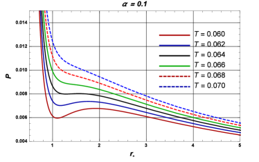
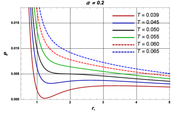
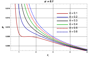
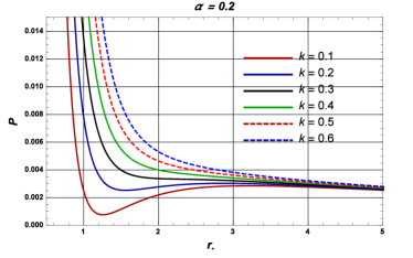
Figure 5: The plot of pressure versus horizon radius for different values of $T_{+}$ and $k$ with $\alpha=0.1$ and $\alpha=0.2$ respectively.

V Connection between phase transition and Shadow radius

To compute the geodesics in the spacetime, we first focus to the motion of photon in the the horizon of black hole solution (14). The Lagrangian for a photon constrained to move in the equatorial plane $(\theta=\pi/2)$ can be expressed as

$${\cal{L}}=-f(r){dt}^{2}+g_{rr}{\dot{r}}^{2}+\frac{1}{f(r)}{d\theta^{2}}+r^{2}{d\phi}^{2}.$$ (44)

The corresponding Hamiltonian is written as

$${\cal{H}}=\frac{1}{2}g^{\mu\nu}p_{\mu}p_{\nu}=\frac{1}{2}\left[-\frac{p_{t}^{2}}{f(r)}+{p_{r}}^{2}f(r)+\frac{p_{\phi}^{2}}{r^{2}}\right].$$ (45)

The equations of motion can be calculated using the Hamiltonian formalism as follows

$${\dot{t}}=\frac{\partial{\cal H}}{\partial p_{t}}=-\frac{p_{t}}{f(r)},\qquad\qquad{\dot{\phi}}=\frac{\partial{\cal H}}{\partial p_{\phi}}=\frac{p_{\phi}}{r^{2}},\quad\text{and}\quad{\dot{r}}=\frac{\partial{\cal H}}{\partial p_{r}}={p_{r}}f(r).$$ (46)

where dot denotes the derivative with respect to affine parameter. Using equations of motion and conserved quantities, the null geodesics equation is given by

$${\dot{r}}^{2}+V_{eff}(r)=0,\qquad\text{with}\qquad V_{eff}=f(r)\left(\frac{J^{2}}{r^{2}}-\frac{E^{2}}{f(r)}\right).$$ (47)

For a circular null geodesics which describes the radius of the photon sphere, the effective potential must follow

$$V_{eff}=0,\qquad\text{and}\qquad\frac{\partial V_{eff}}{\partial r}=0.$$ (48)

The equation of the photon radius ($r_{p}$) can be estimated by Eq. (48). But this equation (48) can not be solve analytically, so we solve it numerically and the values are tabulated in the TABLE 5.

g		0.1		0.3		0.5		0.7
$r_{p}$		0.12		0.099		0.097		0.095
$r_{s}$		0.142		0.098		0.097		0.096
$k$		0.1		0.3		0.5		0.7
$r_{p}$		0.12		0.491		0.711		0.
$r_{s}$		0.142		0.605		0.844		0.
$\alpha$		0.1		0.3		0.5		0.7
$r_{p}$		0.12		0.111		0.108		0.
$r_{s}$		0.142		0.122		0.116		0.

Table 5: The numerical values of photon radius and shadow radius corresponding to different values of magnetic charge, deviation parameter and GB coupling constant.

We can obtain the shadow radius of the black hole. The shadow radius of the black hole is determined by

$$r_{s}=\sqrt{\alpha^{2}+\beta^{2}}=\frac{L_{p}}{E}=\frac{r}{\sqrt{f(r)}}|_{r=r_{p}}.$$ (49)

Here, we plug the value of $f(r)$ (14) into above equation (49) and we substitute the numerical values of $r_{p}$ as presented in TABLE 5. From the TABLE 5, we notice that the photon radius increases with the deviation parameter and decreases with the $g$ and $\alpha$. The celestial coordinates $\alpha$ and $\beta$ Kumar:2019pjp ; Singh:2017vfr ; Ahmed:2022qge ; Ahmed:2020dzj for our black hole solution are given by

$${\bf x}=\lim_{r\to\infty}\left(\frac{rp^{\phi}}{p^{t}}\right),\qquad\text{and}\qquad{\bf y}=\lim_{r\to\infty}\left(\frac{rp^{\theta}}{p^{t}}\right).$$ (50)

The shadow of the obtained solution for different values of magnetic charge $(g)$ and deviation parameter $(k)$ is depicted in FIG. 6.

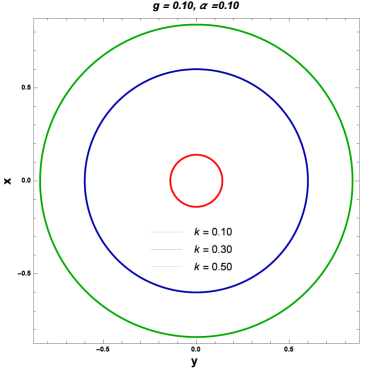
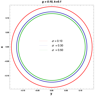
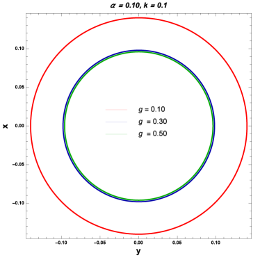
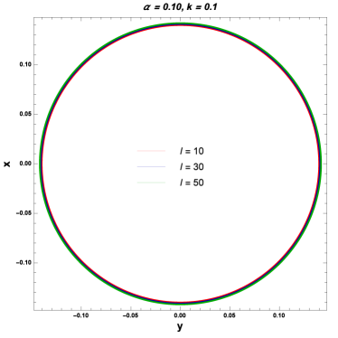
Figure 6: Plot of shadow with different values of deviation parameter $(k)$, magnetic charge $(g)$, GB coupling $(\alpha)$ and length parameter $l$.

From the figure, we observe the effects of different values of deviation parameter $k$, magnetic charge $g$, GB coupling $\alpha$ and cosmological $(\Lambda=-3/l^{2})$ the on the black hole shadow. Here, we find that

1) the size of the shadow increases with increases in the deviation parameter,

2) the size of the shadow decreases with an increase in the magnetic charge and GB coupling constant,

3) and the size of the shadow does not change significantly with increase in the value of $AdS$ length.

VI Conclusions

We have obtained a general $AdS$ regular black hole solution for EGB gravity coupled with non-linear electrodynamics. Interestingly, in the limiting cases, our solution coincides with AdS EGB black hole, Bardeen black hole, AdS regular black hole and AdS Schwarzschild black hole. The horizons of this black hole solution are estimated numerically. We have also analysed the effects of deviation parameter, magnetic charge and GB parameter on the horizon structure. The nature of singularities of obtained solution is also checked by calculating curvature invariants which in turn signifies regular space-time.

Thermodynamics of this general $AdS$ regular black hole solution is also investigated. First of all, we have computed total mass of the system and found that (a) switching off deviation parameter the calculated mass of our system coincides with the mass of the $AdS$ EGB Bardeen black hole Singh:2020xju , (b) switching off magnetic charge this coincides with the mass of $AdS$ EGB regular black hole Singh:2020mty , (c) switching off both the deviation parameter and magnetic charge this identifies to the mass of $4D$ EGB black hole gla , (d) switching off both the GB parameter and deviation parameter this reduces to the mass of Bardeen black hole tzi , (e) switching off both the GB parameter and magnetic charge this reduces to the mass of $AdS$ regular black hole and finally (f) switching all three GB parameter, deviation parameter and magnetic charge this identifies with the mass of $AdS$ Schwarzschild black hole. Furthermore, we have determined Hawking temperature and entropy of the system. The behavior of temperature is also depicted in plots. Moreover, we have studied stability of the system by estimating heat capacity. From the plot, we have observed that heat capacity has discontinuity at a critical radius which signifies a second-order phase transition. At critical radius, the temperature gains its maximum value. This signifies that a phase transition occurs when the size gets bigger.

In addition, $P-v$ criticality of the obtained black hole solution is also discussed. Here, in summery, we found that, even though the critical radius is an increasing function of magnetic charge and decreasing function of deviation parameter, the universal ratio $\frac{P_{C}r_{C}}{T_{C}}$ increases along with both the magnetic charge $g$ and deviation parameter $k$.

Ultimately, in order to discuss black hole shadow, we have estimated the photon radius and shadow radius and their dependence on the different values of magnetic charge and deviation parameter. To study the behavior of black hole shadow, we have plotted diagrams as well.

Data availability statement

Data sharing not applicable to this article as no datasets were generated or analysed during the current study.

References

- (1) B. P. Abbott et al. (Virgo and LIGO Scientific Collaborations), Phys. Rev. Lett. 116 (2016) 061102.
- (2) B. P. Abbott et al. (Virgo and LIGO Scientific Collaborations), Phys. Rev. Lett. 116 (2016) 241102.
- (3) K. Akiyama et al. (Event Horizon Telescope Collaboration), Astrophys. J. 875 (2019) L1.
- (4) T. D. Lee and G. C. Wick, Nucl. Phys. B 9, 209 (1969).
- (5) T. D. Lee and G. C. Wick, Phys. Rev. D 2, 1033 (1970).
- (6) D. V. Singh, S. Upadhyay and S. Ali, Int. J. Mod. Phys. A 37 (2022) 2250049.
- (7) D. Lovelock, J. Math. Phys. 12 (1971) 498.
- (8) C. Lanczos, Ann. Math. 39 (1938) 842.
- (9) B. Zwiebach, Phys. Lett. B 156 (1985) 315.
- (10) D. G. Boulware and S. Deser, Phys. Rev. Lett. 55 (1985) 2656.
- (11) R. G. Cai, Phys. Rev. D 65 (2002) 084014.
- (12) D. Glavan and C. Lin, Phys. Rev. Lett. 124 (2020) 081301.
- (13) M. Gurses, T. C. Sisman and B. Tekin, Phys. Rev. Lett. 125, 149001 (2020).
- (14) K. Aolki, M. A. Gorji and S. Mukohyama, Phys. Lett. B 810, 135843 (2020).
- (15) K. Aolki, M. A. Gorji and S. Mukohyama, JCAP 2009, 014 (2020).
- (16) D. V. Singh, B. K. Singh and S. Upadhyay, Annals Phys. 434 (2021) 168642.
- (17) P. G. S. Fernandes, Phys. Lett. B 805 (2020) 135468.
- (18) S. Upadhyay and D. V. Singh, Eur. Phys. J. Plus 137 (2022) 383.
- (19) N. Godani, D. V. Singh and G. C. Samanta, Phys. Dark Univ. 35 (2022), 100952.
- (20) K. Jusufi, A. Banerjee and S. G. Ghosh, Eur. Phys. J. C 80 (2020) 698.
- (21) G. Panotopoulos, A. Pradhan, T. Tangphati and A. Banerjee, Chin. J. Phys. 77 (2022) 2106.
- (22) T. Tangphati, A. Pradhan, A. Banerjee and G. Panotopoulos, Phys. Dark Univ. 33 (2021) 100877.
- (23) J. M. Z. Pretel, A. Banerjee and A. Pradhan, Eur. Phys. J. C 82 (2022) 180.
- (24) T. Tangphati, A. Pradhan, A. Errehymy and A. Banerjee, Phys. Lett. B 819 (2021) 136423.
- (25) M. Born and L. Infeld, Proc. R. Soc. Lond. 144 (1934) 425.
- (26) E. S. Fradkin and A. A. Tseytlin, Phys. Lett. B 163 (1985) 123.
- (27) E. Bergshoeff, E. Sezgin, C. N. Pope and P. K. Townsend, Phys. Lett. B 188 (1987) 70.
- (28) W. Javed, R. Babar and A. Ovg̈un, Phys. Rev. D ¨ 100 (2019) 104032.
- (29) K. Jusufi, A. Ovg̈un, A. Banerjee and I. Sakalli, Eur. ¨ Phys. J. Plus 134 (2019) 428.
- (30) H. Salazar I., A. Garcia D. and J. Plebanski, J. Math. Phys., 28, 2171 (1987).
- (31) E. Ayon-Beato and A. Garcia, Phys. Rev. Lett. 80, 5056 (1998).
- (32) E. Ayon-Beato and A. Garcia, Gen. Rel. Grav. 31, 629 (1999).
- (33) E. Ayon-Beato, A. Garcia, Phys. Lett. B 493 (2000) 149.
- (34) A. Ovg̈un, Phys. Lett. B 820 (2021) 136517.
- (35) W. Javed, J. Abbas and A. Ovg̈un, Eur. Phys. J. C 79 (2019) 694.
- (36) S. Ali and S. G. Ghosh, Phys. Rev. D 98, 084025 (2018).
- (37) D. V. Singh, S. G. Ghosh and S. D. Maharaj, Annals Phys. 412, 168025 (2019).
- (38) A. Kumar, D. V. Singh and S. G. Ghosh, Eur. Phys. J. C 79, 275 (2019).
- (39) D. V. Singh and S. Siwach, arXiv: 1909.11529 [hep-th].
- (40) J. M. Bardeen, Conference Proceedings of GR5, Tbilisi, USSR, 1968, p. 174.
- (41) J. D. Bekenstein, Phys. Rev. D7 (1973) 2333.
- (42) S. W. Hawking, Comm. Math. Phys. 43 (1975) 19.
- (43) B. L. Hu, Int. J. Mod. Phys. D20 (2011) 697.
- (44) D. V. Singh, S. G. Ghosh and S. D. Maharaj, Nucl. Phys. B 981 (2022) 115854.
- (45) E. Ayon-Beato, A. Garcia, Phys. Lett. B 464, 25 (1999).
- (46) K. A. Bronnikov, Phys. Rev. D 63 (2001) 044005.
- (47) D. V. Singh and S. Siwach, Phys. Lett. B. 408 135658 (2020).
- (48) S. G. Ghosh, D. V. Singh, R. Kumar and S. D. Maharaj, Annals Phys. 424 (2021) 168347.
- (49) A. G. Tzikas, Phys. Lett. B 788 (2019) 219.
- (50) R. Kumar, S. G. Ghosh and A. Wang, Phys. Rev. D 100 (2019) 124024.
- (51) B. P. Singh and S. G. Ghosh, Annals Phys. 395 (2018) 127.
- (52) F. Ahmed, D. V. Singh and S. G. Ghosh, Gen. Rel. Grav. 54 (2022) 21.
- (53) F. Ahmed, D. V. Singh and S. G. Ghosh, arXiv:2008.10241 [gr-qc].