Time Consistency
for Multistage Stochastic Optimization Problems
under Constraints in Expectation

Abstract

We consider sequences — indexed by time (discrete stages) — of families of multistage stochastic optimization problems. At each time, the optimization problems in a family are parameterized by some quantities (initial states, constraint levels…). In this framework, we introduce an adapted notion of time consistent optimal solutions, that is, solutions that remain optimal after truncation of the past and that are optimal for any values of the parameters. We link this time consistency notion with the concept of state variable in Markov Decision Processes for a class of multistage stochastic optimization problems incorporating state constraints at the final time, either formulated in expectation or in probability. For such problems, when the primitive noise random process is stagewise independent and takes a finite number of values, we show that time consistent solutions can be obtained by considering a finite dimensional state variable. We illustrate our results on a simple dam management problem.

Keywords:

Multistage Stochastic Optimization; Time Consistency; Constraints in Expectation; Dynamic Programming

1 Introduction and motivation

The notion of time consistency has been introduced in the field of Economics [11], and developed in the context of risk measures [1, 14, 7, 6]. It has been studied in stochastic optimization, both from the stochastic programming [16, 13] and from the Markov Decision Process [15] points of view. Loosely speaking, time consistency means that strategies obtained by solving the problem at the very first stage do not have to be questioned later on. This definition has been used in [5] to establish links between the concept of state variable and the notion of time consistency. The aim in [5] was to highlight the role of information in time consistency. For example, considering a standard multistage stochastic optimization problem solvable by dynamic programming, it was shown that adding a probabilistic constraint involving the state at the final instant of the time span invalidates the time inconsistency property, in the sense that optimal strategies based on the usual state variable have to be reconsidered at each time stage. It was also shown that it was possible to devise an appropriate state variable, namely the probabilistic distribution of the state variable rather than the state variable itself, to formulate an equivalent problem enjoying the time consistency property. But this state is an infinite dimensional one, so that dynamic programming is usually not implementable. The aim of this article is to give deeper insights into the results established in [5] and to show that it is possible to regain time consistency on such problems by using an extended finite dimensional state variable.

The paper is organized as follows. In Sect. 2, we introduce the notion of universal solution for a family of optimization problems, and we define the notion of time consistency for a sequence of families of optimization problems. Then, we revisit the setting of a discrete time multistage stochastic optimization problem in the standard formulation, and we show that our definition of time consistency applies in this case. In Sect. 3, we add an expectation constraint on the final state to the standard multistage stochastic optimization problem, and we define families of optimization problems parameterized by both the initial state and the level of constraint. We prove that the feedback strategies — obtained by dynamic programming on an extended problem formulation with additional state and control variables — are time consistent. In Sect. 4, we present a toy problem for managing a dam subject to a final constraint in probability, and we give results obtained using the extended formulation. Finally, we draw some conclusions in Sect. 5.

2 Time consistency and multistage stochastic optimization

In §2.1, we introduce the notion of universal solution of a family of optimization problems and the notion of time consistency of a sequence of controls for an optimization data set. In §2.2, we show how these two notions apply in multistage stochastic optimization.

2.1 Universal solutions and time consistency

We start with general considerations on universal solutions and time consistency, before moving to more formal statements.

In optimization, the most natural notion of universal solution is the following. Let $\mathbb{A}$ be a set of parameters and ${\mathbb{U}}$ be a set of (decision) variables. Let $\left\{J^{a}\right\}_{a\in\mathbb{A}}$ be a family of functions $J^{a}:{\mathbb{U}}\to{\mathbb{R}}\cup\{{+\infty}\}$ indexed by the parameter $a$. An element $u^{\sharp}\in{\mathbb{U}}$ is a universal solution for the family of functions $\left\{J^{a}\right\}_{a\in\mathbb{A}}$ when $u^{\sharp}\in\bigcap_{a\in\mathbb{A}}\mathop{\arg\min}_{u\in{\mathbb{U}}}J^{a}({u})$. In a different way, the most natural notion of time consistency in (mutistage) optimization is the following. Let $t_{i}<t_{f}$ be two integers, $\llbracket t_{i},t_{f}\rrbracket=\{{t_{i},t_{i}{+}1,\dots,t_{f}{-}1,t_{f}}\}$ be the corresponding finite time span, and $\left\{{\mathbb{U}}_{t}\right\}_{t\in\llbracket t_{i},t_{f}\rrbracket}$ be a sequence of control sets. We introduce the truncation mapping (projection) at time $t\in\llbracket t_{i},t_{f}\rrbracket$, that is, $\mathfrak{T}_{t}:{\mathbb{U}}_{t_{i}}\times\dots\times{\mathbb{U}}_{t_{f}}\to{\mathbb{U}}_{t}\times\dots\times{\mathbb{U}}_{t_{f}}$ and $\mathfrak{T}_{t}(u_{t_{i}},\ldots,u_{t_{f}})=(u_{t},\ldots,u_{t_{f}})$. Then, considering a sequence of functions $\left\{J_{t}\right\}_{t\in\llbracket t_{i},t_{f}\rrbracket}$, with $J_{t}:{\mathbb{U}}_{t}\times\dots\times{\mathbb{U}}_{t_{f}}\to{\mathbb{R}}\cup\{{+\infty}\}$, we say that time consistency holds when, for all $t\in\llbracket t_{i},t_{f}\rrbracket$,

$$\mathfrak{T}_{t}\big{(}{\mathop{\arg\min}_{({u_{t_{i}},\ldots,u_{t_{f}}})\in{\mathbb{U}}_{t_{i}}\times\dots\times{\mathbb{U}}_{t_{f}}}J_{t_{i}}({u_{t_{i}},\ldots,u_{t_{f}}})}\big{)}\subset\mathop{\arg\min}_{({u_{t},\ldots,u_{t_{f}}})\in{\mathbb{U}}_{t}\times\dots\times{\mathbb{U}}_{t_{f}}}J_{t}({u_{t},\ldots,u_{t_{f}}})\;.$$

We now extend and mix these two notions in the case where the (cost) functions depend on both parameters and time.

Definition 1

We call optimization data set a family $\mathscr{D}=\big{(}\mathcal{T}$, $\{{\mathbb{A}_{t}}\}_{t\in\mathcal{T}}$, $\{{{\mathbb{U}}_{t}}\}_{t\in\mathcal{T}}$, $\{{J_{t}}\}_{t\in\mathcal{T}}\big{)}$, where $\mathcal{T}=\llbracket t_{i},t_{f}\rrbracket$ (with $t_{i}<t_{f}$ two integers), a sequence $\{{\mathbb{A}_{t}}\}_{t\in\mathcal{T}}$ of parameter sets, a sequence $\{{{\mathbb{U}}_{t}}\}_{t\in\mathcal{T}}$ of control sets, a sequence $\{{J_{t}}\}_{t\in\mathcal{T}}$ of cost functions, with $J_{t}:\mathbb{A}_{t}\times\mathbb{U}_{t}\times\dots\times{\mathbb{U}}_{t_{f}}\to\mathbb{R}\cup\{+\infty\}$.

For any $t\in\mathcal{T}$, we call truncated optimization data set at time $t$ the optimization data set $\mathscr{D}_{t}=\big{(}{\llbracket t,t_{f}\rrbracket,\{{\mathbb{A}_{s}}\}_{s\in\llbracket t,t_{f}\rrbracket},\{{{\mathbb{U}}_{s}}\}_{s\in\llbracket t,t_{f}\rrbracket},\{{J_{s}}\}_{s\in\llbracket t,t_{f}\rrbracket}}\big{)}$.

The notion of universal solution for an optimization data set at time $t\in\mathcal{T}$ is the following.

Definition 2

Let ${\mathscr{D}}$ be an optimization data set and let $t\in\mathcal{T}$ be given. We say that $(u_{t}^{\sharp},\dots,u_{t_{f}}^{\sharp})\in{\mathbb{U}}_{t}\times\dots\times{\mathbb{U}}_{t_{f}}$ is a universal solution for the data set ${\mathscr{D}}$ at time $t$ if it satisfies

$$(u_{t}^{\sharp},\dots,u_{t_{f}}^{\sharp})\in\bigcap_{a_{t}\in\mathbb{A}_{t}}\mathop{\arg\min}\big{\{}{\mathscr{P}_{t}^{\mathscr{D}}(a_{t})}\big{\}}\;,$$ (1)

where, for any $a_{t}\in\mathbb{A}_{t}$, the optimization problem $\mathscr{P}_{t}^{\mathscr{D}}(a_{t})$ is defined by

$$\min_{(u_{t},\dots,u_{t_{f}})\in{\mathbb{U}}_{t}\times\dots\times{\mathbb{U}}_{t_{f}}}\;J_{t}(a_{t},u_{t},\dots,u_{t_{f}})\;.$$ (2)

The property of time consistency of a sequence $(u_{t_{i}}^{\sharp},\dots,u_{t_{f}}^{\sharp})$ of controls for an optimization data set $\mathscr{D}$ is defined as follows.

Definition 3

Let $\mathscr{D}$ be an optimization data set and let $(u_{t_{i}}^{\sharp},\dots,u_{t_{f}}^{\sharp})$ be a sequence of controls in ${\mathbb{U}}_{t_{i}}\times\dots\times{\mathbb{U}}_{t_{f}}$. We say that the sequence $(u_{t_{i}}^{\sharp},\dots,u_{t_{f}}^{\sharp})$ of controls is time consistent for the optimization data set $\mathscr{D}$ if, for any $t\in\mathcal{T}$, the truncated subsequence $(u_{t}^{\sharp},\dots,u_{t_{f}}^{\sharp})=\mathfrak{T}_{t}(u_{t_{i}}^{\sharp},\dots,u_{t_{f}}^{\sharp})$ of controls is a universal solution for the optimization data set ${\mathscr{D}}$ at time $t$.

Otherwise stated, given a universal solution $(u_{t_{i}}^{\sharp},\dots,u_{t_{f}}^{\sharp})$ for the data set ${\mathscr{D}}$ at initial time $t_{i}$, time consistency means that the subsequence $(u_{t}^{\sharp},\dots,u_{t_{f}}^{\sharp})$ is a universal solution for the data set ${\mathscr{D}}$ at time $t$, for any time $t>t_{i}$.

2.2 Multistage stochastic optimization in the classical case

We study the standard case of a controlled dynamical system influenced by exogenous disturbances. The decision maker has to find strategies to drive the system so as to minimize some objective function over a certain time span.

Let be given a probability space $(\Omega,{\cal F},\mathbb{P})$. All random variables and all random processes are defined on $(\Omega,{\cal F},\mathbb{P})$, and we denote them using bold letters. We denote by $\sigma({\boldsymbol{Z^{\textstyle\text{\unboldmath$\scriptstyle$}}_{\textstyle\text{\unboldmath$\scriptstyle$}}}})\subset{\cal F}$ the $\sigma$-field generated by a random variable $\boldsymbol{Z^{\textstyle\text{\unboldmath$\scriptstyle$}}_{\textstyle\text{\unboldmath$\scriptstyle$}}}$.

We consider a positive integer $T>0$ and the finite time span $\llbracket 0,T\rrbracket=\{0$, $1$, $\dots$,$T{-}1$, $T\}$. We denote by $\boldsymbol{W^{\textstyle\text{\unboldmath$\scriptstyle$}}_{\textstyle\text{\unboldmath$\scriptstyle$}}}=\{{\boldsymbol{W^{\textstyle\text{\unboldmath$\scriptstyle$}}_{\textstyle\text{\unboldmath$\scriptstyle t$}}}}\}_{t=1,\dots,T}$ the primitive (or exogenous) noise random process, where each random variable $\boldsymbol{W^{\textstyle\text{\unboldmath$\scriptstyle$}}_{\textstyle\text{\unboldmath$\scriptstyle t$}}}$ takes values in a measurable space $\mathbb{W}_{t}$. We denote by $\boldsymbol{U^{\textstyle\text{\unboldmath$\scriptstyle$}}_{\textstyle\text{\unboldmath$\scriptstyle$}}}=\{{\boldsymbol{U^{\textstyle\text{\unboldmath$\scriptstyle$}}_{\textstyle\text{\unboldmath$\scriptstyle t$}}}}\}_{t=0,\dots,T{-}1}$ the control random process, where each random variable $\boldsymbol{U^{\textstyle\text{\unboldmath$\scriptstyle$}}_{\textstyle\text{\unboldmath$\scriptstyle t$}}}$ takes values in a measurable space $\mathbb{U}_{t}$, and by $\boldsymbol{X^{\textstyle\text{\unboldmath$\scriptstyle$}}_{\textstyle\text{\unboldmath$\scriptstyle$}}}=\{{\boldsymbol{X^{\textstyle\text{\unboldmath$\scriptstyle$}}_{\textstyle\text{\unboldmath$\scriptstyle t$}}}}\}_{t=0,\dots,T}$ the state random process, where each random variable $\boldsymbol{X^{\textstyle\text{\unboldmath$\scriptstyle$}}_{\textstyle\text{\unboldmath$\scriptstyle t$}}}$ takes values in a measurable space $\mathbb{X}_{t}$. We consider a sequence $\{{f_{t}}\}_{t=0,\dots,T{-}1}$ of measurable mappings $f_{t}:\mathbb{X}_{t}\times\mathbb{U}_{t}\times\mathbb{W}_{t+1}\rightarrow\mathbb{X}_{t+1}$ (dynamics), a sequence $\{{L_{t}}\}_{t=0,\dots,T{-}1}$ of measurable functions $L_{t}:\mathbb{X}_{t}\times\mathbb{U}_{t}\times\mathbb{W}_{t+1}\rightarrow{\mathbb{R}}_{+}\cup\{{+\infty}\}$ (instantaneous cost), and a measurable function $K:\mathbb{X}_{T+1}\rightarrow{\mathbb{R}}_{+}\cup\{{+\infty}\}$ (final cost).

The optimization problem we consider below consists in minimizing the expectation of a sum of costs depending on the state, the control and the noise variables over the finite time span $\llbracket 0,T\rrbracket$. The state variable evolves with respect to the dynamics $f_{t}$ that depends on the current state, noise and control values. The problem starting at time $t=0$ is

$$\min_{\boldsymbol{U^{\textstyle\text{\unboldmath$\scriptstyle$}}_{\textstyle\text{\unboldmath$\scriptstyle$}}},\boldsymbol{X^{\textstyle\text{\unboldmath$\scriptstyle$}}_{\textstyle\text{\unboldmath$\scriptstyle$}}}}\quad {{\mathbb{E}}}\bigg{[}{\sum_{t=0}^{T{-}1}L_{t}({\boldsymbol{X^{\textstyle\text{\unboldmath$\scriptstyle$}}_{\textstyle\text{\unboldmath$\scriptstyle t$}}},\boldsymbol{U^{\textstyle\text{\unboldmath$\scriptstyle$}}_{\textstyle\text{\unboldmath$\scriptstyle t$}}},\boldsymbol{W^{\textstyle\text{\unboldmath$\scriptstyle$}}_{\textstyle\text{\unboldmath$\scriptstyle t+1$}}}})+K({\boldsymbol{X^{\textstyle\text{\unboldmath$\scriptstyle$}}_{\textstyle\text{\unboldmath$\scriptstyle T$}}}})}\bigg{]}\;,$$ (3a)

s.t. $$\boldsymbol{X^{\textstyle\text{\unboldmath$\scriptstyle$}}_{\textstyle\text{\unboldmath$\scriptstyle 0$}}}=x_{0}\;,$$ (3b)

$$\boldsymbol{X^{\textstyle\text{\unboldmath$\scriptstyle$}}_{\textstyle\text{\unboldmath$\scriptstyle t+1$}}}=f_{t}({\boldsymbol{X^{\textstyle\text{\unboldmath$\scriptstyle$}}_{\textstyle\text{\unboldmath$\scriptstyle t$}}},\boldsymbol{U^{\textstyle\text{\unboldmath$\scriptstyle$}}_{\textstyle\text{\unboldmath$\scriptstyle t$}}},\boldsymbol{W^{\textstyle\text{\unboldmath$\scriptstyle$}}_{\textstyle\text{\unboldmath$\scriptstyle t+1$}}}})\;,\enspace\qquad\forall t=0,\dots,T{-}1\;,$$ (3c)

$$\sigma({\boldsymbol{U^{\textstyle\text{\unboldmath$\scriptstyle$}}_{\textstyle\text{\unboldmath$\scriptstyle t$}}}})\subset\sigma({\boldsymbol{W^{\textstyle\text{\unboldmath$\scriptstyle$}}_{\textstyle\text{\unboldmath$\scriptstyle 1$}}},\dots,\boldsymbol{W^{\textstyle\text{\unboldmath$\scriptstyle$}}_{\textstyle\text{\unboldmath$\scriptstyle t$}}}})\;,\enspace\qquad\;\forall t=0,\dots,T{-}1\;.$$ (3d)

By convention, for $t=0$, the $\sigma$-field $\sigma({\boldsymbol{W^{\textstyle\text{\unboldmath$\scriptstyle$}}_{\textstyle\text{\unboldmath$\scriptstyle 1$}}},\dots,\boldsymbol{W^{\textstyle\text{\unboldmath$\scriptstyle$}}_{\textstyle\text{\unboldmath$\scriptstyle t$}}}})$ is the trivial $\sigma$-field $\{{\emptyset,\Omega}\}$. Under the measurability assumptions made, Problem (3) is well-defined as all functions take extended nonnegative values.

We make the following assumption.

Assumption 1 (Markovian setting)

The noise random variables $\boldsymbol{W^{\textstyle\text{\unboldmath$\scriptstyle$}}_{\textstyle\text{\unboldmath$\scriptstyle 1$}}},\dots,\boldsymbol{W^{\textstyle\text{\unboldmath$\scriptstyle$}}_{\textstyle\text{\unboldmath$\scriptstyle T$}}}$ are independent.

Using Assumption 1, it is well known [2] that there is no loss of optimality in looking for the optimal control $\boldsymbol{U^{\textstyle\text{\unboldmath$\scriptstyle$}}_{\textstyle\text{\unboldmath$\scriptstyle t$}}}$ at time $t$ of Problem (3) as a feedback strategy depending on the state variable $\boldsymbol{X^{\textstyle\text{\unboldmath$\scriptstyle$}}_{\textstyle\text{\unboldmath$\scriptstyle t$}}}$, that is, as a measurable mapping $\phi_{t}:\mathbb{X}_{t}\rightarrow\mathbb{U}_{t}$ (state feedback).

Let us embed Problem (3) in the framework developed in §2.1. For that purpose, we build an optimization data set

$$\mathscr{S}=\big{(}{\mathcal{T},\{{\mathbb{X}_{t}}\}_{t\in\mathcal{T}},\{{\mathcal{U}_{t}}\}_{t\in\mathcal{T}},\{{J_{t}}\}_{t\in\mathcal{T}}}\big{)}\;.$$ (4)

The discrete time span $\mathcal{T}$ is $\llbracket 0,T{-}1\rrbracket$, the sequence of parameter sets is $\{{\mathbb{X}_{t}}\}_{t\in\mathcal{T}}$, and the sequence of control spaces is $\{{\mathcal{U}_{t}}\}_{t\in\mathcal{T}}$, $\mathcal{U}_{t}$ being the space of measurable mappings $\phi_{t}:\mathbb{X}_{t}\rightarrow\mathbb{U}_{t}$ (state feedbacks). The sequence $\{{J_{t}}\}_{t\in\mathcal{T}}$ of cost functions

$$J_{t}\;:\; \mathbb{X}_{t}\times\mathcal{U}_{t}\times\dots\times\mathcal{U}_{T{-}1}\;\longrightarrow\;\mathbb{R}\cup\{+\infty\}$$

$$\quad(x_{t},\phi_{t},\dots,\phi_{T{-}1})\quad\longmapsto\;J_{t}(x_{t},\phi_{t},\dots,\phi_{T{-}1})\;,$$

is defined by

$$J_{t}(x_{t},\phi_{t},\dots,\phi_{T{-}1})=\; {{\mathbb{E}}}\bigg{[}{\sum_{\tau=t}^{T{-}1}L_{\tau}\big{(}{\boldsymbol{X^{\textstyle\text{\unboldmath$\scriptstyle$}}_{\textstyle\text{\unboldmath$\scriptstyle\tau$}}},\phi_{\tau}({\boldsymbol{X^{\textstyle\text{\unboldmath$\scriptstyle$}}_{\textstyle\text{\unboldmath$\scriptstyle\tau$}}}}),\boldsymbol{W^{\textstyle\text{\unboldmath$\scriptstyle$}}_{\textstyle\text{\unboldmath$\scriptstyle\tau+1$}}}}\big{)}+K({\boldsymbol{X^{\textstyle\text{\unboldmath$\scriptstyle$}}_{\textstyle\text{\unboldmath$\scriptstyle T$}}}})}\bigg{]}\;,$$

with $$\boldsymbol{X^{\textstyle\text{\unboldmath$\scriptstyle$}}_{\textstyle\text{\unboldmath$\scriptstyle t$}}}=x_{t}\;,$$

$$\boldsymbol{X^{\textstyle\text{\unboldmath$\scriptstyle$}}_{\textstyle\text{\unboldmath$\scriptstyle\tau+1$}}}=f_{\tau}\big{(}{\boldsymbol{X^{\textstyle\text{\unboldmath$\scriptstyle$}}_{\textstyle\text{\unboldmath$\scriptstyle\tau$}}},\phi_{\tau}({\boldsymbol{X^{\textstyle\text{\unboldmath$\scriptstyle$}}_{\textstyle\text{\unboldmath$\scriptstyle\tau$}}}}),\boldsymbol{W^{\textstyle\text{\unboldmath$\scriptstyle$}}_{\textstyle\text{\unboldmath$\scriptstyle\tau+1$}}}}\big{)}\;,\enspace\forall\tau\in\llbracket t,T{-}1\rrbracket\;.$$

Thanks to dynamic programming, we obtain the following result. The sequence $({\phi_{0}^{\sharp},\dots,\phi_{T{-}1}^{\sharp}})$ of optimal strategies of Problem (3), obtained by solving the dynamic programming equation backward in time

$$V_{T}(x) =K(x)\;,$$ (5a)

$$V_{t}(x) =\min_{u\in\mathbb{U}_{t}}{{\mathbb{E}}}\Big{[}{L_{t}(x,u,\boldsymbol{W^{\textstyle\text{\unboldmath$\scriptstyle$}}_{\textstyle\text{\unboldmath$\scriptstyle t+1$}}})+V_{t+1}\big{(}{f_{t}(x,u,\boldsymbol{W^{\textstyle\text{\unboldmath$\scriptstyle$}}_{\textstyle\text{\unboldmath$\scriptstyle t+1$}}})}\big{)}}\Big{]}\;,$$ (5b)

with

$$\phi_{t}^{\sharp}(x) \in\mathop{\arg\min}_{u\in\mathbb{U}_{t}}{{\mathbb{E}}}\Big{[}{L_{t}(x,u,\boldsymbol{W^{\textstyle\text{\unboldmath$\scriptstyle$}}_{\textstyle\text{\unboldmath$\scriptstyle t+1$}}})+V_{t+1}\big{(}{f_{t}(x,u,\boldsymbol{W^{\textstyle\text{\unboldmath$\scriptstyle$}}_{\textstyle\text{\unboldmath$\scriptstyle t+1$}}})}\big{)}}\Big{]}\;,$$ (5c)

is time consistent, in the sense of Definition 3, for the optimization data set ${\cal S}$ defined in Equation (4). Indeed, letting time $t\in\mathcal{T}$ be given, we build from the data set ${\cal S}$ the family $\mathscr{P}_{t}^{\mathscr{S}}=\big{\{}{\mathscr{P}_{t}^{\mathscr{S}}(x_{t})}\big{\}}_{x_{t}\in\mathbb{X}_{t}}$ of optimization problems as in Equation (2), with Problem $\mathscr{P}_{t}^{\mathscr{S}}(x_{t})$ being

$$\min_{(\phi_{t},\dots,\phi_{T{-}1})\in\mathcal{U}_{t}\times\dots\times\mathcal{U}_{T{-}1}}\;J_{t}(x_{t},\phi_{t},\dots,\phi_{T{-}1})\;.$$ (6)

It is clear that Problem $\mathscr{P}_{0}^{\mathscr{S}}(x_{0})$ coincides with Problem (3). From the Bellman theory, we know that the sequence $({\phi_{0}^{\sharp},\dots,\phi_{T{-}1}^{\sharp}})$ of strategies obtained by solving the dynamic programming equation (5) is such that, for any $t\in\mathcal{T}$, the truncated sequence $({\phi_{t}^{\sharp},\dots,\phi_{T{-}1}^{\sharp}})$ is an optimal solution of Problem (6) for any initial state $x_{t}$. Thus, according to Definition 3, the sequence $({\phi_{0}^{\sharp},\dots,\phi_{T{-}1}^{\sharp}})$ of controls is time consistent for the optimization data set $\mathscr{S}$.

Remark 4

The notion of time consistency crucially depends on the nature of the solutions of the family of optimization problem under consideration. As a matter of fact, consider Problem (3) and its solution $(\phi_{0}^{\sharp},\dots,\phi_{T{-}1}^{\sharp})$ in terms of feedback strategies: as already explained, there is no difficulty to apply the truncated sequence $(\phi_{t}^{\sharp},\dots,\phi_{T{-}1}^{\sharp})$ to Problem (6) since this truncated sequence is admissible for the problem starting at time $t$. But consider again Problem (3) and its solution $\boldsymbol{U^{\textstyle\text{\unboldmath$\scriptstyle$}}_{\textstyle\text{\unboldmath$\scriptstyle$}}}^{\sharp}=(\boldsymbol{U^{\textstyle\text{\unboldmath$\scriptstyle$}}_{\textstyle\text{\unboldmath$\scriptstyle$}}}^{\sharp}_{0},\ldots,\boldsymbol{U^{\textstyle\text{\unboldmath$\scriptstyle$}}_{\textstyle\text{\unboldmath$\scriptstyle$}}}^{\sharp}_{T{-}1})$ in terms of random variables. Problem (6) is equivalent to

$$\min_{\boldsymbol{U^{\textstyle\text{\unboldmath$\scriptstyle$}}_{\textstyle\text{\unboldmath$\scriptstyle$}}},\boldsymbol{X^{\textstyle\text{\unboldmath$\scriptstyle$}}_{\textstyle\text{\unboldmath$\scriptstyle$}}}}\quad {{\mathbb{E}}}\bigg{[}{\sum_{\tau=t}^{T{-}1}L_{\tau}({\boldsymbol{X^{\textstyle\text{\unboldmath$\scriptstyle$}}_{\textstyle\text{\unboldmath$\scriptstyle\tau$}}},\boldsymbol{U^{\textstyle\text{\unboldmath$\scriptstyle$}}_{\textstyle\text{\unboldmath$\scriptstyle\tau$}}},\boldsymbol{W^{\textstyle\text{\unboldmath$\scriptstyle$}}_{\textstyle\text{\unboldmath$\scriptstyle\tau+1$}}}})+K({\boldsymbol{X^{\textstyle\text{\unboldmath$\scriptstyle$}}_{\textstyle\text{\unboldmath$\scriptstyle T$}}}})}\bigg{]}\;,$$ (7a)

s.t. $$\boldsymbol{X^{\textstyle\text{\unboldmath$\scriptstyle$}}_{\textstyle\text{\unboldmath$\scriptstyle t$}}}=x_{t}\;,$$ (7b)

$$\boldsymbol{X^{\textstyle\text{\unboldmath$\scriptstyle$}}_{\textstyle\text{\unboldmath$\scriptstyle\tau+1$}}}=f_{\tau}({\boldsymbol{X^{\textstyle\text{\unboldmath$\scriptstyle$}}_{\textstyle\text{\unboldmath$\scriptstyle\tau$}}},\boldsymbol{U^{\textstyle\text{\unboldmath$\scriptstyle$}}_{\textstyle\text{\unboldmath$\scriptstyle\tau$}}},\boldsymbol{W^{\textstyle\text{\unboldmath$\scriptstyle$}}_{\textstyle\text{\unboldmath$\scriptstyle\tau+1$}}}})\;,\enspace\qquad\forall\tau\in\llbracket t,T{-}1\rrbracket\;,$$ (7c)

$$\sigma({\boldsymbol{U^{\textstyle\text{\unboldmath$\scriptstyle$}}_{\textstyle\text{\unboldmath$\scriptstyle\tau$}}}})\subset\sigma({\boldsymbol{W^{\textstyle\text{\unboldmath$\scriptstyle$}}_{\textstyle\text{\unboldmath$\scriptstyle t+1$}}},\dots,\boldsymbol{W^{\textstyle\text{\unboldmath$\scriptstyle$}}_{\textstyle\text{\unboldmath$\scriptstyle\tau$}}}})\;,\enspace\qquad\forall\tau\in\llbracket t,T{-}1\rrbracket\;.$$ (7d)

We note that the truncated subsequence $(\boldsymbol{U^{\textstyle\text{\unboldmath$\scriptstyle$}}_{\textstyle\text{\unboldmath$\scriptstyle$}}}^{\sharp}_{t},\ldots,\boldsymbol{U^{\textstyle\text{\unboldmath$\scriptstyle$}}_{\textstyle\text{\unboldmath$\scriptstyle$}}}^{\sharp}_{T{-}1})$ of $\boldsymbol{U^{\textstyle\text{\unboldmath$\scriptstyle$}}_{\textstyle\text{\unboldmath$\scriptstyle$}}}^{\sharp}$ is not even admissible for Problem 7 as it does not satisfy (7d). Indeed, each $\boldsymbol{U^{\textstyle\text{\unboldmath$\scriptstyle$}}_{\textstyle\text{\unboldmath$\scriptstyle$}}}^{\sharp}_{\tau}$ for $\tau\in\llbracket t,T{-}1\rrbracket$ is by construction (see Constraint (3d)) measurable with respect to the $\sigma$-field $\sigma(\boldsymbol{W^{\textstyle\text{\unboldmath$\scriptstyle$}}_{\textstyle\text{\unboldmath$\scriptstyle 1$}}}$, $\ldots$, $\boldsymbol{W^{\textstyle\text{\unboldmath$\scriptstyle$}}_{\textstyle\text{\unboldmath$\scriptstyle\tau$}}})$ and thus does not satisfy Constraint (7d).

3 Multistage stochastic optimization with a final constraint in expectation

In §3.1, we modify the framework studied in §2.2 by adding to Problem (3) a constraint in expectation involving the final state $\boldsymbol{X^{\textstyle\text{\unboldmath$\scriptstyle$}}_{\textstyle\text{\unboldmath$\scriptstyle T$}}}$, which leads to the optimization problem (8) below. In §3.2, we propose a reformulation of Problem (8) involving a finite dimensional state, and an optimization data set (including the initial state and the level of the expectation constraint) for which time consistency holds. In §3.3, we propose a dual problem formulation of Problem (8), and we illustrate the fact that such a reformulation is not time consistent.

3.1 Standard formulation

We use the notations defined in §2.2. We consider a measurable function $g:\mathbb{X}_{T}\to\mathbb{R}_{+}^{m}$, For convenience, we denote $\mathbb{Z}_{T}=\mathbb{R}^{m}$. The stochastic optimization problem starting at time $t_{0}\in\llbracket 0,T{-}1\rrbracket$ with a final constraint in expectation at time $T$ is

$$\min_{\boldsymbol{U^{\textstyle\text{\unboldmath$\scriptstyle$}}_{\textstyle\text{\unboldmath$\scriptstyle$}}},\boldsymbol{X^{\textstyle\text{\unboldmath$\scriptstyle$}}_{\textstyle\text{\unboldmath$\scriptstyle$}}}}\quad {{\mathbb{E}}}\bigg{[}{\sum_{t=t_{0}}^{T{-}1}L_{t}\big{(}{\boldsymbol{X^{\textstyle\text{\unboldmath$\scriptstyle$}}_{\textstyle\text{\unboldmath$\scriptstyle t$}}},\boldsymbol{U^{\textstyle\text{\unboldmath$\scriptstyle$}}_{\textstyle\text{\unboldmath$\scriptstyle t$}}},\boldsymbol{W^{\textstyle\text{\unboldmath$\scriptstyle$}}_{\textstyle\text{\unboldmath$\scriptstyle t+1$}}}}\big{)}+K({\boldsymbol{X^{\textstyle\text{\unboldmath$\scriptstyle$}}_{\textstyle\text{\unboldmath$\scriptstyle T$}}}})}\bigg{]}\;,$$ (8a)

s.t. $$\boldsymbol{X^{\textstyle\text{\unboldmath$\scriptstyle$}}_{\textstyle\text{\unboldmath$\scriptstyle t_{0}$}}}=x_{t_{0}}\;,$$ (8b)

$$\boldsymbol{X^{\textstyle\text{\unboldmath$\scriptstyle$}}_{\textstyle\text{\unboldmath$\scriptstyle t+1$}}}=f_{t}\big{(}{\boldsymbol{X^{\textstyle\text{\unboldmath$\scriptstyle$}}_{\textstyle\text{\unboldmath$\scriptstyle t$}}},\boldsymbol{U^{\textstyle\text{\unboldmath$\scriptstyle$}}_{\textstyle\text{\unboldmath$\scriptstyle t$}}},\boldsymbol{W^{\textstyle\text{\unboldmath$\scriptstyle$}}_{\textstyle\text{\unboldmath$\scriptstyle t+1$}}}}\big{)}\;,\enspace\qquad\quad\;\forall t\in\llbracket t_{0},T{-}1\rrbracket\;,$$ (8c)

$$\sigma\big{(}{\boldsymbol{U^{\textstyle\text{\unboldmath$\scriptstyle$}}_{\textstyle\text{\unboldmath$\scriptstyle t$}}}}\big{)}\subset\sigma\big{(}{\boldsymbol{W^{\textstyle\text{\unboldmath$\scriptstyle$}}_{\textstyle\text{\unboldmath$\scriptstyle t_{0}{+}1$}}},\dots,\boldsymbol{W^{\textstyle\text{\unboldmath$\scriptstyle$}}_{\textstyle\text{\unboldmath$\scriptstyle t$}}}}\big{)}\;,\enspace\qquad\;\forall t\in\llbracket t_{0},T{-}1\rrbracket\;,$$ (8d)

$${{\mathbb{E}}}\big{[}{g(\boldsymbol{X^{\textstyle\text{\unboldmath$\scriptstyle$}}_{\textstyle\text{\unboldmath$\scriptstyle T$}}})}\big{]}-b_{t_{0}}\leq 0\;,$$ (8e)

with $b_{t_{0}}\in\mathbb{R}^{m}$. Again, Problem (8) is assumed to be well-defined.

Even under the Markovian Assumption 1, the presence of Constraint (8e) makes it difficult to write a dynamic programming equation for solving Problem (8) starting at time $t_{0}=0$. Indeed Constraint (8e) is not a pointwise constraint at the final stage $T$, so that we do not know how to incorporate it easily in the dynamic programming equation. In §3.3, using an indirect way of proceeding, we show that it is possible to obtain an optimal solution of Problem (8) starting at time $t_{0}=0$ in terms of feedback strategies depending on the state $\boldsymbol{X^{\textstyle\text{\unboldmath$\scriptstyle$}}_{\textstyle\text{\unboldmath$\scriptstyle t$}}}$. But these feedbacks are implicitly parameterized by both the initial state $x_{0}$ and the constraint level $b_{0}$, so that they do not satisfy the time consistency property for a data set in which the parameter at time $t$ is the initial state $x_{t}$ (see §3.3 for further details).

A partial answer to the question of time consistency of the solution of Problem (8) starting at time $t_{0}=0$ has been given in [5]. Indeed, as detailed in [5], Problem (8) can be written in an equivalent way as a deterministic distributed optimal control problem in which the state variable is the probability distribution of $\boldsymbol{X^{\textstyle\text{\unboldmath$\scriptstyle$}}_{\textstyle\text{\unboldmath$\scriptstyle t$}}}$, the dynamics of which is given by the Fokker-Planck equation. This deterministic problem can be solved by dynamic programming, which thus produces a sequence $(\Psi_{0}^{\sharp},\dots,\Psi_{T{-}1}^{\sharp})$ of strategies (with the mapping $\Psi_{t}$ defined over probability distributions on $\mathbb{X}_{t}$ and taking values in $\mathbb{U}_{t}$ [3]), which is time consistent for a data set in which the parameter at time $t$ is the initial state probability distribution. But these optimal strategies depend on the specific value $b_{0}$ in the right-hand side of the expectation constraint, and thus have to be recomputed if this value changes. Moreover, the computation of the Bellman functions involves an infinite dimensional state, so that it is generally not tractable.

Our goal is to obtain a solution for Problem (8) starting at time $t_{0}=0$ which, on the one hand is computable in practice (that is, involves a finite dimensional state), and on the other hand is time consistent for a data set (to be specified) in which the parameter at time $t$ consists of both the initial state $x_{t}$ and the constraint level $b_{t}$. More precisely, we want to compute a solution for Problem (8) starting at time $t_{0}=0$ which is optimal for any value of both the initial state $x_{0}$ in (8b) and the final constraint level $b_{0}$ in (8e). Moreover, for any $t\in\llbracket 0,T{-}1\rrbracket$, this solution after truncation has to be a universal solution (Definition 2) for the parameters $(x_{t},b_{t})$ for Problem (8) starting at $t_{0}=t$. As already explained in Remark 4, time consistency is not available for a solution in terms of random variables. We now present a reformulation of Problem (8) involving a finite dimensional state, whose solution in terms of state feedback strategies meets the goal described in this paragraph.

3.2 Formulation with martingale-type constraints

Following the same path as in [4], but in a discrete time context, we show that Problem (8) is equivalent to a multistage stochastic optimization problem subject to an almost sure contraint on the final state (see also [9, 10, 12]). For that purpose, we introduce a new state process $\boldsymbol{Z^{\textstyle\text{\unboldmath$\scriptstyle$}}_{\textstyle\text{\unboldmath$\scriptstyle$}}}=(\boldsymbol{Z^{\textstyle\text{\unboldmath$\scriptstyle$}}_{\textstyle\text{\unboldmath$\scriptstyle 0$}}},\ldots,\boldsymbol{Z^{\textstyle\text{\unboldmath$\scriptstyle$}}_{\textstyle\text{\unboldmath$\scriptstyle T$}}})$ and a new control process $\boldsymbol{V^{\textstyle\text{\unboldmath$\scriptstyle$}}_{\textstyle\text{\unboldmath$\scriptstyle$}}}=(\boldsymbol{V^{\textstyle\text{\unboldmath$\scriptstyle$}}_{\textstyle\text{\unboldmath$\scriptstyle 0$}}},\ldots,\boldsymbol{V^{\textstyle\text{\unboldmath$\scriptstyle$}}_{\textstyle\text{\unboldmath$\scriptstyle T{-}1$}}})$. The random variables $\boldsymbol{Z^{\textstyle\text{\unboldmath$\scriptstyle$}}_{\textstyle\text{\unboldmath$\scriptstyle t$}}}$ and $\boldsymbol{V^{\textstyle\text{\unboldmath$\scriptstyle$}}_{\textstyle\text{\unboldmath$\scriptstyle t$}}}$ take their values respectively in spaces $\mathbb{V}_{t}$ and $\mathbb{Z}_{t}$, all identical to the space $\mathbb{Z}_{T}=\mathbb{R}^{m}$ where $\mathbb{R}^{m}$ is the codomain of the function $g$ introduced at the beginning of §3.1: $\mathbb{V}_{t}=\mathbb{Z}_{t}=\mathbb{Z}_{T}=\mathbb{R}^{m}$ for all $t\in\llbracket 0,T{-}1\rrbracket$. Now, we consider the optimization problem starting at time $t_{0}$

$$\min_{(\boldsymbol{U^{\textstyle\text{\unboldmath$\scriptstyle$}}_{\textstyle\text{\unboldmath$\scriptstyle$}}},\boldsymbol{V^{\textstyle\text{\unboldmath$\scriptstyle$}}_{\textstyle\text{\unboldmath$\scriptstyle$}}},\boldsymbol{X^{\textstyle\text{\unboldmath$\scriptstyle$}}_{\textstyle\text{\unboldmath$\scriptstyle$}}},\boldsymbol{Z^{\textstyle\text{\unboldmath$\scriptstyle$}}_{\textstyle\text{\unboldmath$\scriptstyle$}}})}\; {{\mathbb{E}}}\bigg{[}{\sum_{t=t_{0}}^{T{-}1}L_{t}(\boldsymbol{X^{\textstyle\text{\unboldmath$\scriptstyle$}}_{\textstyle\text{\unboldmath$\scriptstyle t$}}},\boldsymbol{U^{\textstyle\text{\unboldmath$\scriptstyle$}}_{\textstyle\text{\unboldmath$\scriptstyle t$}}},\boldsymbol{W^{\textstyle\text{\unboldmath$\scriptstyle$}}_{\textstyle\text{\unboldmath$\scriptstyle t+1$}}})+K(\boldsymbol{X^{\textstyle\text{\unboldmath$\scriptstyle$}}_{\textstyle\text{\unboldmath$\scriptstyle T$}}})}\bigg{]}\;,$$ (9a)

subject, for all $$t=t_{0},\dots,T{-}1$$, to dynamic constraints

$$\boldsymbol{X^{\textstyle\text{\unboldmath$\scriptstyle$}}_{\textstyle\text{\unboldmath$\scriptstyle t_{0}$}}}=x_{t_{0}}\;,\enspace\quad\boldsymbol{X^{\textstyle\text{\unboldmath$\scriptstyle$}}_{\textstyle\text{\unboldmath$\scriptstyle t+1$}}}=f_{t}(\boldsymbol{X^{\textstyle\text{\unboldmath$\scriptstyle$}}_{\textstyle\text{\unboldmath$\scriptstyle t$}}},\boldsymbol{U^{\textstyle\text{\unboldmath$\scriptstyle$}}_{\textstyle\text{\unboldmath$\scriptstyle t$}}},\boldsymbol{W^{\textstyle\text{\unboldmath$\scriptstyle$}}_{\textstyle\text{\unboldmath$\scriptstyle t+1$}}})\;,$$ (9b)

$$\boldsymbol{Z^{\textstyle\text{\unboldmath$\scriptstyle$}}_{\textstyle\text{\unboldmath$\scriptstyle t_{0}$}}}=z_{t_{0}}\;,\enspace\quad\;\boldsymbol{Z^{\textstyle\text{\unboldmath$\scriptstyle$}}_{\textstyle\text{\unboldmath$\scriptstyle t+1$}}}=\boldsymbol{Z^{\textstyle\text{\unboldmath$\scriptstyle$}}_{\textstyle\text{\unboldmath$\scriptstyle t$}}}+\boldsymbol{V^{\textstyle\text{\unboldmath$\scriptstyle$}}_{\textstyle\text{\unboldmath$\scriptstyle t$}}}\;,$$ (9c)

to measurability constraints

$$\sigma\big{(}{\boldsymbol{U^{\textstyle\text{\unboldmath$\scriptstyle$}}_{\textstyle\text{\unboldmath$\scriptstyle t$}}}}\big{)}\subset\sigma\big{(}{\boldsymbol{W^{\textstyle\text{\unboldmath$\scriptstyle$}}_{\textstyle\text{\unboldmath$\scriptstyle t_{0}{+}1$}}},\dots,\boldsymbol{W^{\textstyle\text{\unboldmath$\scriptstyle$}}_{\textstyle\text{\unboldmath$\scriptstyle t$}}}}\big{)}\;,$$ (9d)

$$\sigma\big{(}{\boldsymbol{V^{\textstyle\text{\unboldmath$\scriptstyle$}}_{\textstyle\text{\unboldmath$\scriptstyle t$}}}}\big{)}\subset\sigma\big{(}{\boldsymbol{W^{\textstyle\text{\unboldmath$\scriptstyle$}}_{\textstyle\text{\unboldmath$\scriptstyle t_{0}{+}1$}}},\dots,\boldsymbol{W^{\textstyle\text{\unboldmath$\scriptstyle$}}_{\textstyle\text{\unboldmath$\scriptstyle t+1$}}}}\big{)}\;,$$ (9e)

to martingale-type constraints

$$\boldsymbol{V^{\textstyle\text{\unboldmath$\scriptstyle$}}_{\textstyle\text{\unboldmath$\scriptstyle t$}}}\text{ is integrable and }{\mathbb{E}}\big{[}{\boldsymbol{V^{\textstyle\text{\unboldmath$\scriptstyle$}}_{\textstyle\text{\unboldmath$\scriptstyle t$}}}\,\big{|}\,\sigma({\boldsymbol{W^{\textstyle\text{\unboldmath$\scriptstyle$}}_{\textstyle\text{\unboldmath$\scriptstyle t_{0}{+}1$}}},\dots,\boldsymbol{W^{\textstyle\text{\unboldmath$\scriptstyle$}}_{\textstyle\text{\unboldmath$\scriptstyle t$}}}})}\big{]}=0\;,$$ (9f)

and to almost sure final constraint

$$g(\boldsymbol{X^{\textstyle\text{\unboldmath$\scriptstyle$}}_{\textstyle\text{\unboldmath$\scriptstyle T$}}})-\boldsymbol{Z^{\textstyle\text{\unboldmath$\scriptstyle$}}_{\textstyle\text{\unboldmath$\scriptstyle T$}}}\leq 0\;.$$ (9g)

Note that, in this formulation, the control variable $\boldsymbol{U^{\textstyle\text{\unboldmath$\scriptstyle$}}_{\textstyle\text{\unboldmath$\scriptstyle t$}}}$ taken at time $t$ does not depend on the noise $\boldsymbol{W^{\textstyle\text{\unboldmath$\scriptstyle$}}_{\textstyle\text{\unboldmath$\scriptstyle t+1$}}}$ (Decision–Hazard framework), whereas the control variable $\boldsymbol{V^{\textstyle\text{\unboldmath$\scriptstyle$}}_{\textstyle\text{\unboldmath$\scriptstyle t$}}}$, also taken at time $t$, does depend on the noise $\boldsymbol{W^{\textstyle\text{\unboldmath$\scriptstyle$}}_{\textstyle\text{\unboldmath$\scriptstyle t+1$}}}$ (Hazard–Decision framework). At time $t$, the martingale-type constraint (9f) introduces a coupling between all the realizations of the decision random variable $\boldsymbol{V^{\textstyle\text{\unboldmath$\scriptstyle$}}_{\textstyle\text{\unboldmath$\scriptstyle t$}}}$. In the sequel, for all $t\in\llbracket t_{0}{+}1,T\rrbracket$, we denote by $\mathcal{F}_{t_{0}:t}$ the $\sigma$-field generated by the sequence $(\boldsymbol{W^{\textstyle\text{\unboldmath$\scriptstyle$}}_{\textstyle\text{\unboldmath$\scriptstyle t_{0}{+}1$}}},\dots,\boldsymbol{W^{\textstyle\text{\unboldmath$\scriptstyle$}}_{\textstyle\text{\unboldmath$\scriptstyle t$}}})$ of random variables:

$$\mathcal{F}_{t_{0}:t}=\sigma\big{(}{\boldsymbol{W^{\textstyle\text{\unboldmath$\scriptstyle$}}_{\textstyle\text{\unboldmath$\scriptstyle t_{0}{+}1$}}},\dots,\boldsymbol{W^{\textstyle\text{\unboldmath$\scriptstyle$}}_{\textstyle\text{\unboldmath$\scriptstyle t$}}}}\big{)}\;.$$ (10)

By convention, $\mathcal{F}_{t_{0}:t_{0}}=\{{\emptyset,\Omega}\}$.

3.2.1 Equivalence with the standard formulation

The link between the multistage stochastic optimization control problem (9) incorporating a martingale-type constraint and the initial problem (8) is given by the following proposition.

Proposition 5

We suppose that the data of the Problems (8) and (9) are linked by

$$b_{t_{0}}=z_{t_{0}}\;.$$ (11)

Then, Problem (8) and Problem (9) are equivalent, in the sense that

• a solution $(\boldsymbol{U^{\textstyle\text{\unboldmath$\scriptstyle\flat$}}_{\textstyle\text{\unboldmath$\scriptstyle$}}},\boldsymbol{V^{\textstyle\text{\unboldmath$\scriptstyle\flat$}}_{\textstyle\text{\unboldmath$\scriptstyle$}}},\boldsymbol{X^{\textstyle\text{\unboldmath$\scriptstyle\flat$}}_{\textstyle\text{\unboldmath$\scriptstyle$}}},\boldsymbol{Z^{\textstyle\text{\unboldmath$\scriptstyle\flat$}}_{\textstyle\text{\unboldmath$\scriptstyle$}}})$ of Problem (9) can be deduced from a solution $(\boldsymbol{U^{\textstyle\text{\unboldmath$\scriptstyle$}}_{\textstyle\text{\unboldmath$\scriptstyle$}}}^{\sharp},\boldsymbol{X^{\textstyle\text{\unboldmath$\scriptstyle$}}_{\textstyle\text{\unboldmath$\scriptstyle$}}}^{\sharp})$ of Problem (8),

• the two first components $(\boldsymbol{U^{\textstyle\text{\unboldmath$\scriptstyle\flat$}}_{\textstyle\text{\unboldmath$\scriptstyle$}}},\boldsymbol{X^{\textstyle\text{\unboldmath$\scriptstyle\flat$}}_{\textstyle\text{\unboldmath$\scriptstyle$}}})$ of a solution $(\boldsymbol{U^{\textstyle\text{\unboldmath$\scriptstyle\flat$}}_{\textstyle\text{\unboldmath$\scriptstyle$}}},\boldsymbol{V^{\textstyle\text{\unboldmath$\scriptstyle\flat$}}_{\textstyle\text{\unboldmath$\scriptstyle$}}},\boldsymbol{X^{\textstyle\text{\unboldmath$\scriptstyle\flat$}}_{\textstyle\text{\unboldmath$\scriptstyle$}}},\boldsymbol{Z^{\textstyle\text{\unboldmath$\scriptstyle\flat$}}_{\textstyle\text{\unboldmath$\scriptstyle$}}})$ of Problem (9) is a solution of Problem (8).

Proof. Let $(\boldsymbol{U^{\textstyle\text{\unboldmath$\scriptstyle$}}_{\textstyle\text{\unboldmath$\scriptstyle$}}}^{\sharp},\boldsymbol{X^{\textstyle\text{\unboldmath$\scriptstyle$}}_{\textstyle\text{\unboldmath$\scriptstyle$}}}^{\sharp})$ be a solution of Problem (8). We define the random processes $\boldsymbol{V^{\textstyle\text{\unboldmath$\scriptstyle$}}_{\textstyle\text{\unboldmath$\scriptstyle$}}}^{\sharp}$ and $\boldsymbol{Z^{\textstyle\text{\unboldmath$\scriptstyle$}}_{\textstyle\text{\unboldmath$\scriptstyle$}}}^{\sharp}$ by

$$\boldsymbol{V^{\textstyle\text{\unboldmath$\scriptstyle$}}_{\textstyle\text{\unboldmath$\scriptstyle$}}}^{\sharp}_{t}={\mathbb{E}}\big{[}{g(\boldsymbol{X^{\textstyle\text{\unboldmath$\scriptstyle$}}_{\textstyle\text{\unboldmath$\scriptstyle$}}}^{\sharp}_{T})\,\big{|}\,\mathcal{F}_{t_{0}:t+1}}\big{]}-{\mathbb{E}}\big{[}{g(\boldsymbol{X^{\textstyle\text{\unboldmath$\scriptstyle$}}_{\textstyle\text{\unboldmath$\scriptstyle$}}}^{\sharp}_{T})\,\big{|}\,\mathcal{F}_{t_{0}:t}}\big{]}\;,\enspace\quad\forall t\in\llbracket t_{0},T{-}1\rrbracket\;,$$ (12a)

$$\boldsymbol{Z^{\textstyle\text{\unboldmath$\scriptstyle$}}_{\textstyle\text{\unboldmath$\scriptstyle$}}}^{\sharp}_{t_{0}}=z_{t_{0}}\;,\enspace\quad\boldsymbol{Z^{\textstyle\text{\unboldmath$\scriptstyle$}}_{\textstyle\text{\unboldmath$\scriptstyle$}}}^{\sharp}_{t+1}=\boldsymbol{Z^{\textstyle\text{\unboldmath$\scriptstyle$}}_{\textstyle\text{\unboldmath$\scriptstyle$}}}^{\sharp}_{t}+\boldsymbol{V^{\textstyle\text{\unboldmath$\scriptstyle$}}_{\textstyle\text{\unboldmath$\scriptstyle$}}}^{\sharp}_{t}\;,\enspace\qquad\qquad\qquad\;\forall t\in\llbracket t_{0},T{-}1\rrbracket\;.$$ (12b)

The random vector $\boldsymbol{V^{\textstyle\text{\unboldmath$\scriptstyle$}}_{\textstyle\text{\unboldmath$\scriptstyle$}}}^{\sharp}_{t}$ is well defined (hence so is $\boldsymbol{Z^{\textstyle\text{\unboldmath$\scriptstyle$}}_{\textstyle\text{\unboldmath$\scriptstyle$}}}^{\sharp}_{t}$) and is integrable. Indeed, as the function $g:\mathbb{X}_{T}\to\mathbb{R}_{+}^{m}$ is assumed nonnegative in §3.1 and using Inequality (8e), we get $0\leq{{\mathbb{E}}}[{g(\boldsymbol{X^{\textstyle\text{\unboldmath$\scriptstyle$}}_{\textstyle\text{\unboldmath$\scriptstyle$}}}^{\sharp}_{T})}]\leq b_{t_{0}}$. As $b_{t_{0}}\in\mathbb{R}^{m}$, the random vector $g(\boldsymbol{X^{\textstyle\text{\unboldmath$\scriptstyle$}}_{\textstyle\text{\unboldmath$\scriptstyle$}}}^{\sharp}_{T})$ is integrable, hence $\boldsymbol{V^{\textstyle\text{\unboldmath$\scriptstyle$}}_{\textstyle\text{\unboldmath$\scriptstyle$}}}^{\sharp}_{t}$ in (12a) is the difference between two random vectors in $\mathbb{R}^{m}$, hence is well defined, and is integrable.

By construction, the two processes $\boldsymbol{V^{\textstyle\text{\unboldmath$\scriptstyle$}}_{\textstyle\text{\unboldmath$\scriptstyle$}}}^{\sharp}$ and $\boldsymbol{Z^{\textstyle\text{\unboldmath$\scriptstyle$}}_{\textstyle\text{\unboldmath$\scriptstyle$}}}^{\sharp}$ satisfy the constraints (9c)–(9e)–(9f). Moreover, we have that

$$\boldsymbol{Z^{\textstyle\text{\unboldmath$\scriptstyle$}}_{\textstyle\text{\unboldmath$\scriptstyle$}}}^{\sharp}_{T} =z_{t_{0}}+\sum_{t=t_{0}}^{T{-}1}\boldsymbol{V^{\textstyle\text{\unboldmath$\scriptstyle$}}_{\textstyle\text{\unboldmath$\scriptstyle$}}}^{\sharp}_{t}$$ (by (12b))

$$=z_{t_{0}}+g(\boldsymbol{X^{\textstyle\text{\unboldmath$\scriptstyle$}}_{\textstyle\text{\unboldmath$\scriptstyle$}}}^{\sharp}_{T})-{{\mathbb{E}}}[{g(\boldsymbol{X^{\textstyle\text{\unboldmath$\scriptstyle$}}_{\textstyle\text{\unboldmath$\scriptstyle$}}}^{\sharp}_{T})}]\;,$$ (by telescoping sum using (12a))

and hence, by (8e) and (11), we get that

$$g(\boldsymbol{X^{\textstyle\text{\unboldmath$\scriptstyle$}}_{\textstyle\text{\unboldmath$\scriptstyle$}}}^{\sharp}_{T})-\boldsymbol{Z^{\textstyle\text{\unboldmath$\scriptstyle$}}_{\textstyle\text{\unboldmath$\scriptstyle$}}}^{\sharp}_{T}={{\mathbb{E}}}\big{[}{g(\boldsymbol{X^{\textstyle\text{\unboldmath$\scriptstyle$}}_{\textstyle\text{\unboldmath$\scriptstyle$}}}^{\sharp}_{T})}\big{]}-z_{t_{0}}\leq b_{t_{0}}-z_{t_{0}}=0\;,$$

so that Constraint (9g) is also fulfilled. We deduce that $(\boldsymbol{U^{\textstyle\text{\unboldmath$\scriptstyle$}}_{\textstyle\text{\unboldmath$\scriptstyle$}}}^{\sharp},\boldsymbol{V^{\textstyle\text{\unboldmath$\scriptstyle$}}_{\textstyle\text{\unboldmath$\scriptstyle$}}}^{\sharp},\boldsymbol{X^{\textstyle\text{\unboldmath$\scriptstyle$}}_{\textstyle\text{\unboldmath$\scriptstyle$}}}^{\sharp},\boldsymbol{Z^{\textstyle\text{\unboldmath$\scriptstyle$}}_{\textstyle\text{\unboldmath$\scriptstyle$}}}^{\sharp})$ is admissible for Problem (9). Suppose that there would exist a solution $(\boldsymbol{U^{\textstyle\text{\unboldmath$\scriptstyle\flat$}}_{\textstyle\text{\unboldmath$\scriptstyle$}}},\boldsymbol{V^{\textstyle\text{\unboldmath$\scriptstyle\flat$}}_{\textstyle\text{\unboldmath$\scriptstyle$}}},\boldsymbol{X^{\textstyle\text{\unboldmath$\scriptstyle\flat$}}_{\textstyle\text{\unboldmath$\scriptstyle$}}},\boldsymbol{Z^{\textstyle\text{\unboldmath$\scriptstyle\flat$}}_{\textstyle\text{\unboldmath$\scriptstyle$}}})$ of Problem (9) with a strictly lower cost value than $(\boldsymbol{U^{\textstyle\text{\unboldmath$\scriptstyle$}}_{\textstyle\text{\unboldmath$\scriptstyle$}}}^{\sharp},\boldsymbol{V^{\textstyle\text{\unboldmath$\scriptstyle$}}_{\textstyle\text{\unboldmath$\scriptstyle$}}}^{\sharp},\boldsymbol{X^{\textstyle\text{\unboldmath$\scriptstyle$}}_{\textstyle\text{\unboldmath$\scriptstyle$}}}^{\sharp},\boldsymbol{Z^{\textstyle\text{\unboldmath$\scriptstyle$}}_{\textstyle\text{\unboldmath$\scriptstyle$}}}^{\sharp})$. From the dynamics (9c), we would have

$$\boldsymbol{Z^{\textstyle\text{\unboldmath$\scriptstyle\flat$}}_{\textstyle\text{\unboldmath$\scriptstyle T$}}}=z_{t_{0}}+\sum_{t=t_{0}}^{T{-}1}\boldsymbol{V^{\textstyle\text{\unboldmath$\scriptstyle\flat$}}_{\textstyle\text{\unboldmath$\scriptstyle t$}}}\;,$$

so that ${{\mathbb{E}}}[{\boldsymbol{Z^{\textstyle\text{\unboldmath$\scriptstyle\flat$}}_{\textstyle\text{\unboldmath$\scriptstyle T$}}}}]=z_{t_{0}}$ by repeated uses of (9f). Taking the expectation in (9g) would lead thus to

$${{\mathbb{E}}}\big{[}{g(\boldsymbol{X^{\textstyle\text{\unboldmath$\scriptstyle\flat$}}_{\textstyle\text{\unboldmath$\scriptstyle T$}}})}\big{]}\leq{{\mathbb{E}}}[{\boldsymbol{Z^{\textstyle\text{\unboldmath$\scriptstyle\flat$}}_{\textstyle\text{\unboldmath$\scriptstyle T$}}}}]=z_{t_{0}}=b_{t_{0}}\;.$$

Then, $(\boldsymbol{U^{\textstyle\text{\unboldmath$\scriptstyle\flat$}}_{\textstyle\text{\unboldmath$\scriptstyle$}}},\boldsymbol{X^{\textstyle\text{\unboldmath$\scriptstyle\flat$}}_{\textstyle\text{\unboldmath$\scriptstyle$}}})$ would be admissible for Problem (8) with a strictly lower cost value than the optimal solution $(\boldsymbol{U^{\textstyle\text{\unboldmath$\scriptstyle$}}_{\textstyle\text{\unboldmath$\scriptstyle$}}}^{\sharp},\boldsymbol{X^{\textstyle\text{\unboldmath$\scriptstyle$}}_{\textstyle\text{\unboldmath$\scriptstyle$}}}^{\sharp})$, which contradicts the assumed optimality of $(\boldsymbol{U^{\textstyle\text{\unboldmath$\scriptstyle$}}_{\textstyle\text{\unboldmath$\scriptstyle$}}}^{\sharp},\boldsymbol{X^{\textstyle\text{\unboldmath$\scriptstyle$}}_{\textstyle\text{\unboldmath$\scriptstyle$}}}^{\sharp})$. We conclude that $(\boldsymbol{U^{\textstyle\text{\unboldmath$\scriptstyle$}}_{\textstyle\text{\unboldmath$\scriptstyle$}}}^{\sharp},\boldsymbol{V^{\textstyle\text{\unboldmath$\scriptstyle$}}_{\textstyle\text{\unboldmath$\scriptstyle$}}}^{\sharp},\boldsymbol{X^{\textstyle\text{\unboldmath$\scriptstyle$}}_{\textstyle\text{\unboldmath$\scriptstyle$}}}^{\sharp},\boldsymbol{Z^{\textstyle\text{\unboldmath$\scriptstyle$}}_{\textstyle\text{\unboldmath$\scriptstyle$}}}^{\sharp})$ is an optimal solution of Problem (9).

Conversely, let $(\boldsymbol{U^{\textstyle\text{\unboldmath$\scriptstyle\flat$}}_{\textstyle\text{\unboldmath$\scriptstyle$}}},\boldsymbol{V^{\textstyle\text{\unboldmath$\scriptstyle\flat$}}_{\textstyle\text{\unboldmath$\scriptstyle$}}},\boldsymbol{X^{\textstyle\text{\unboldmath$\scriptstyle\flat$}}_{\textstyle\text{\unboldmath$\scriptstyle$}}},\boldsymbol{Z^{\textstyle\text{\unboldmath$\scriptstyle\flat$}}_{\textstyle\text{\unboldmath$\scriptstyle$}}})$ be an optimal solution of Problem (9). As shown in the first part of the proof, we have ${{\mathbb{E}}}\big{[}{g(\boldsymbol{X^{\textstyle\text{\unboldmath$\scriptstyle\flat$}}_{\textstyle\text{\unboldmath$\scriptstyle T$}}})}\big{]}\leq b_{t_{0}}$, so that $(\boldsymbol{U^{\textstyle\text{\unboldmath$\scriptstyle\flat$}}_{\textstyle\text{\unboldmath$\scriptstyle$}}},\boldsymbol{X^{\textstyle\text{\unboldmath$\scriptstyle\flat$}}_{\textstyle\text{\unboldmath$\scriptstyle$}}})$ is admissible for Problem (8). Suppose that there would exist a solution $(\boldsymbol{U^{\textstyle\text{\unboldmath$\scriptstyle$}}_{\textstyle\text{\unboldmath$\scriptstyle$}}}^{\sharp},\boldsymbol{X^{\textstyle\text{\unboldmath$\scriptstyle$}}_{\textstyle\text{\unboldmath$\scriptstyle$}}}^{\sharp})$ of Problem (8) with a strictly lower cost value than $(\boldsymbol{U^{\textstyle\text{\unboldmath$\scriptstyle\flat$}}_{\textstyle\text{\unboldmath$\scriptstyle$}}},\boldsymbol{X^{\textstyle\text{\unboldmath$\scriptstyle\flat$}}_{\textstyle\text{\unboldmath$\scriptstyle$}}})$. Then, the quadruplet $(\boldsymbol{U^{\textstyle\text{\unboldmath$\scriptstyle$}}_{\textstyle\text{\unboldmath$\scriptstyle$}}}^{\sharp},\boldsymbol{V^{\textstyle\text{\unboldmath$\scriptstyle$}}_{\textstyle\text{\unboldmath$\scriptstyle$}}}^{\sharp},\boldsymbol{X^{\textstyle\text{\unboldmath$\scriptstyle$}}_{\textstyle\text{\unboldmath$\scriptstyle$}}}^{\sharp},\boldsymbol{Z^{\textstyle\text{\unboldmath$\scriptstyle$}}_{\textstyle\text{\unboldmath$\scriptstyle$}}}^{\sharp})$ obtained by constructing $\boldsymbol{V^{\textstyle\text{\unboldmath$\scriptstyle$}}_{\textstyle\text{\unboldmath$\scriptstyle$}}}^{\sharp}$ and $\boldsymbol{Z^{\textstyle\text{\unboldmath$\scriptstyle$}}_{\textstyle\text{\unboldmath$\scriptstyle$}}}^{\sharp}$ by (12) would give a strictly lower cost value for Problem (9) than $(\boldsymbol{U^{\textstyle\text{\unboldmath$\scriptstyle\flat$}}_{\textstyle\text{\unboldmath$\scriptstyle$}}},\boldsymbol{V^{\textstyle\text{\unboldmath$\scriptstyle\flat$}}_{\textstyle\text{\unboldmath$\scriptstyle$}}},\boldsymbol{X^{\textstyle\text{\unboldmath$\scriptstyle\flat$}}_{\textstyle\text{\unboldmath$\scriptstyle$}}},\boldsymbol{Z^{\textstyle\text{\unboldmath$\scriptstyle\flat$}}_{\textstyle\text{\unboldmath$\scriptstyle$}}})$, which would be absurd. We conclude that $(\boldsymbol{U^{\textstyle\text{\unboldmath$\scriptstyle\flat$}}_{\textstyle\text{\unboldmath$\scriptstyle$}}},\boldsymbol{X^{\textstyle\text{\unboldmath$\scriptstyle\flat$}}_{\textstyle\text{\unboldmath$\scriptstyle$}}})$ is an optimal solution of Problem (8). $\Box$

Let us make a few comments about Problem (9).

• The nice features of the equivalent formulation (9) of Problem (8) are double. On the one hand, the initial constraint (8e) in expectation is replaced by an almost sure constraint (9g) on the final state, hence paving the way to use dynamic programming to solve Problem (9). On the other hand, the parameter defining the right-hand side of the constraint (8e) in expectation in formulation (8) becomes a component (9c) of the initial state in Problem (9), thus leading to time consistency as a consequence of dynamic programming.

• The conditional expectation ${\mathbb{E}}\big{[}{g(\boldsymbol{X^{\textstyle\text{\unboldmath$\scriptstyle$}}_{\textstyle\text{\unboldmath$\scriptstyle T$}}})\,\big{|}\,\mathcal{F}_{t_{0}:t}}\big{]}$ can be interpreted as the “perception of the risk constraint (8e)” at time $t$. From the very definition of $\boldsymbol{V^{\textstyle\text{\unboldmath$\scriptstyle$}}_{\textstyle\text{\unboldmath$\scriptstyle t$}}}$, we have that

  $$\boldsymbol{V^{\textstyle\text{\unboldmath$\scriptstyle$}}_{\textstyle\text{\unboldmath$\scriptstyle t$}}}={\mathbb{E}}\big{[}{g(\boldsymbol{X^{\textstyle\text{\unboldmath$\scriptstyle$}}_{\textstyle\text{\unboldmath$\scriptstyle T$}}})\,\big{|}\,\mathcal{F}_{t_{0}:t+1}}\big{]}-{\mathbb{E}}\big{[}{g(\boldsymbol{X^{\textstyle\text{\unboldmath$\scriptstyle$}}_{\textstyle\text{\unboldmath$\scriptstyle T$}}})\,\big{|}\,\mathcal{F}_{t_{0}:t}}\big{]}\;,$$

  from which we deduce that the control $\boldsymbol{V^{\textstyle\text{\unboldmath$\scriptstyle$}}_{\textstyle\text{\unboldmath$\scriptstyle t$}}}$ corresponds to the variation of this perception between time $t$ and time $t+1$. The additional state $\boldsymbol{Z^{\textstyle\text{\unboldmath$\scriptstyle$}}_{\textstyle\text{\unboldmath$\scriptstyle t+1$}}}$ in (9c) is thus the cumulative variation of the risk contraint perception up to time $t+1$. Therefore, this new added state seems to be the minimal information which has to be added to the standard state in order to recover a dynamic programming principle.

• Nevertheless, Problem (9) is rather more intricate that Problem (8):

  1. there are additional state and control processes $\boldsymbol{Z^{\textstyle\text{\unboldmath$\scriptstyle$}}_{\textstyle\text{\unboldmath$\scriptstyle$}}}$ and $\boldsymbol{V^{\textstyle\text{\unboldmath$\scriptstyle$}}_{\textstyle\text{\unboldmath$\scriptstyle$}}}$,

  2. the new control variables $\boldsymbol{V^{\textstyle\text{\unboldmath$\scriptstyle$}}_{\textstyle\text{\unboldmath$\scriptstyle t$}}}$ has to be searched in the Hazard–Decision framework as in (9e),

  3. a new expectation constraint (9f) on the controls $\boldsymbol{V^{\textstyle\text{\unboldmath$\scriptstyle$}}_{\textstyle\text{\unboldmath$\scriptstyle t$}}}$ appears at each time step.

3.2.2 Extended dynamic programming equation and time consistency

The interest of Problem (9) is highlighted by the following theorem.

Theorem 6

Suppose that the primitive noise random process $\boldsymbol{W^{\textstyle\text{\unboldmath$\scriptstyle$}}_{\textstyle\text{\unboldmath$\scriptstyle$}}}$ = $(\boldsymbol{W^{\textstyle\text{\unboldmath$\scriptstyle$}}_{\textstyle\text{\unboldmath$\scriptstyle 1$}}}$, $\ldots$, $\boldsymbol{W^{\textstyle\text{\unboldmath$\scriptstyle$}}_{\textstyle\text{\unboldmath$\scriptstyle T$}}})$ takes a finite number of values, and that the following induction (Bellman equation)

$$\mathscr{V}_{T}(x,z)=\; K(x)+\chi_{{}_{\{{g(x)-z\leq 0}\}}}(x,z)\;,$$ (13a)

$$\mathscr{V}_{t}(x,z)=\; \min_{u}\;\min_{\begin{subarray}{c}\sigma({\boldsymbol{V^{\textstyle\text{\unboldmath$\scriptstyle$}}_{\textstyle\text{\unboldmath$\scriptstyle$}}}})\subset\sigma({\boldsymbol{W^{\textstyle\text{\unboldmath$\scriptstyle$}}_{\textstyle\text{\unboldmath$\scriptstyle t+1$}}}})\\ {{\mathbb{E}}}[{\boldsymbol{V^{\textstyle\text{\unboldmath$\scriptstyle$}}_{\textstyle\text{\unboldmath$\scriptstyle$}}}}]=0\end{subarray}}\;{{\mathbb{E}}}\Big{[}{L_{t}(x,u,\boldsymbol{W^{\textstyle\text{\unboldmath$\scriptstyle$}}_{\textstyle\text{\unboldmath$\scriptstyle t+1$}}})+\mathscr{V}_{t+1}\big{(}{f_{t}(x,u,\boldsymbol{W^{\textstyle\text{\unboldmath$\scriptstyle$}}_{\textstyle\text{\unboldmath$\scriptstyle t+1$}}}),z+\boldsymbol{V^{\textstyle\text{\unboldmath$\scriptstyle$}}_{\textstyle\text{\unboldmath$\scriptstyle$}}}}\big{)}}\Big{]}$$ (13b)

is well-defined in the sense that all the functions $\mathscr{V}_{t}:\mathbb{X}_{t}\times\mathbb{Z}_{t}\to{\mathbb{R}}_{+}\cup\{{+\infty}\}$ are measurable, for $t\in\llbracket 0,T\rrbracket$.

Then, under Assumption 1, Problem (9) starting at time $t_{0}=0$ can be solved by dynamic programming with associated Bellman equation (13), and its optimal value is $\mathscr{V}_{0}(x_{0},z_{0})$.

Proof. The proof of Theorem 6 in given in Appendix B. $\Box$

We deduce from Equation (13) that there is no loss of optimality in looking for the optimal control $\boldsymbol{U^{\textstyle\text{\unboldmath$\scriptstyle$}}_{\textstyle\text{\unboldmath$\scriptstyle t$}}}$ at time $t$ of Problem (9) as induced by a measurable mapping $\phi_{t}:\mathbb{X}_{t}\times\mathbb{Z}_{t}\rightarrow\mathbb{U}_{t}$, and for the optimal control $\boldsymbol{V^{\textstyle\text{\unboldmath$\scriptstyle$}}_{\textstyle\text{\unboldmath$\scriptstyle t+1$}}}$ at time $t$ as induced by a measurable mapping $\varphi_{t}:\mathbb{X}_{t}\times\mathbb{Z}_{t}\times\mathbb{W}_{t+1}\rightarrow\mathbb{V}_{t}$.

Let us embed Problem (9) starting at time $t_{0}=0$ in the framework developed in §2.1. The finite time span is $\mathcal{T}=\llbracket 0,T{-}1\rrbracket$, the sequence of parameter sets is $\{{\mathbb{X}_{t}\times\mathbb{Z}_{t}}\}_{t\in\mathcal{T}}$, the sequences of control spaces are made of two sequences, $\{{\mathcal{U}_{t}}\}_{t\in\mathcal{T}}$ with $\mathcal{U}_{t}$ the space of measurable mappings defined on $\mathbb{X}_{t}\times\mathbb{Z}_{t}$ and taking values in $\mathbb{U}_{t}$, and $\{{\mathcal{V}_{t}}\}_{t\in\mathcal{T}}$ with $\mathcal{V}_{t}$ the space of measurable mappings defined on $\mathbb{X}_{t}\times\mathbb{Z}_{t}\times\mathbb{W}_{t+1}$ and taking values in $\mathbb{V}_{t}$. Notice that there exists an additional set $\mathbb{X}_{T}\times\mathbb{Z}_{T}$, where the final state of the system takes values, but that this set is not part of the sequence of parameter sets. The sequence of cost functions $\{{J_{t}}\}_{t\in\mathcal{T}}$, with

$$J_{t}\;:\; \mathbb{X}_{t}\times\mathbb{Z}_{t}\times\mathcal{U}_{t}\times\mathcal{V}_{t}\times\dots\times\mathcal{U}_{T{-}1}\times\mathcal{V}_{T{-}1}\,\longrightarrow\;\mathbb{R}\;,$$

is defined by

$$J_{t}(x_{t} ,z_{t},\phi_{t},\varphi_{t},\dots,\phi_{T{-}1},\varphi_{T{-}1})=\;{\mathbb{E}}\bigg{(}\sum_{\tau=t}^{T{-}1}L_{\tau}\big{(}{\boldsymbol{X^{\textstyle\text{\unboldmath$\scriptstyle$}}_{\textstyle\text{\unboldmath$\scriptstyle\tau$}}},\phi_{\tau}(\boldsymbol{X^{\textstyle\text{\unboldmath$\scriptstyle$}}_{\textstyle\text{\unboldmath$\scriptstyle\tau$}}},\boldsymbol{Z^{\textstyle\text{\unboldmath$\scriptstyle$}}_{\textstyle\text{\unboldmath$\scriptstyle\tau$}}}),\boldsymbol{W^{\textstyle\text{\unboldmath$\scriptstyle$}}_{\textstyle\text{\unboldmath$\scriptstyle\tau+1$}}}}\big{)}$$

$$\hphantom{,z_{t},\phi_{t},\varphi_{t},\dots,\phi_{T{-}1},\varphi_{T{-}1})=\;{\mathbb{E}}\bigg{(}\sum_{\tau=t}^{T{-}1}}+K({\boldsymbol{X^{\textstyle\text{\unboldmath$\scriptstyle$}}_{\textstyle\text{\unboldmath$\scriptstyle T$}}}})+\chi_{{}_{\{{g(x)-z\leq 0}\}}}(\boldsymbol{X^{\textstyle\text{\unboldmath$\scriptstyle$}}_{\textstyle\text{\unboldmath$\scriptstyle T$}}},\boldsymbol{Z^{\textstyle\text{\unboldmath$\scriptstyle$}}_{\textstyle\text{\unboldmath$\scriptstyle T$}}})\bigg{)}\;,$$

$$\text{ with }\;\boldsymbol{X^{\textstyle\text{\unboldmath$\scriptstyle$}}_{\textstyle\text{\unboldmath$\scriptstyle t$}}}=x_{t}\;,\enspace\boldsymbol{X^{\textstyle\text{\unboldmath$\scriptstyle$}}_{\textstyle\text{\unboldmath$\scriptstyle\tau+1$}}}=f_{\tau}\big{(}{\boldsymbol{X^{\textstyle\text{\unboldmath$\scriptstyle$}}_{\textstyle\text{\unboldmath$\scriptstyle\tau$}}},\phi_{\tau}(\boldsymbol{X^{\textstyle\text{\unboldmath$\scriptstyle$}}_{\textstyle\text{\unboldmath$\scriptstyle\tau$}}},\boldsymbol{Z^{\textstyle\text{\unboldmath$\scriptstyle$}}_{\textstyle\text{\unboldmath$\scriptstyle\tau$}}}),\boldsymbol{W^{\textstyle\text{\unboldmath$\scriptstyle$}}_{\textstyle\text{\unboldmath$\scriptstyle\tau+1$}}}}\big{)}\;,\enspace\text{ for }\tau\in\llbracket t,T{-}1\rrbracket\;,$$

$$\hphantom{\text{ with }\;}\boldsymbol{Z^{\textstyle\text{\unboldmath$\scriptstyle$}}_{\textstyle\text{\unboldmath$\scriptstyle t$}}}=z_{t}\;,\enspace\boldsymbol{Z^{\textstyle\text{\unboldmath$\scriptstyle$}}_{\textstyle\text{\unboldmath$\scriptstyle\tau+1$}}}=\boldsymbol{Z^{\textstyle\text{\unboldmath$\scriptstyle$}}_{\textstyle\text{\unboldmath$\scriptstyle\tau$}}}+\varphi_{\tau}(\boldsymbol{X^{\textstyle\text{\unboldmath$\scriptstyle$}}_{\textstyle\text{\unboldmath$\scriptstyle\tau$}}},\boldsymbol{Z^{\textstyle\text{\unboldmath$\scriptstyle$}}_{\textstyle\text{\unboldmath$\scriptstyle\tau$}}},\boldsymbol{W^{\textstyle\text{\unboldmath$\scriptstyle$}}_{\textstyle\text{\unboldmath$\scriptstyle\tau+1$}}})\;,\enspace\text{ for }\tau\in\llbracket t,T{-}1\rrbracket\;,$$

if $${\mathbb{E}}\Big{[}{\varphi_{\tau}(\boldsymbol{X^{\textstyle\text{\unboldmath$\scriptstyle$}}_{\textstyle\text{\unboldmath$\scriptstyle\tau$}}},\boldsymbol{Z^{\textstyle\text{\unboldmath$\scriptstyle$}}_{\textstyle\text{\unboldmath$\scriptstyle\tau$}}},\boldsymbol{W^{\textstyle\text{\unboldmath$\scriptstyle$}}_{\textstyle\text{\unboldmath$\scriptstyle\tau+1$}}})\,\Big{|}\,\boldsymbol{X^{\textstyle\text{\unboldmath$\scriptstyle$}}_{\textstyle\text{\unboldmath$\scriptstyle\tau$}}},\boldsymbol{Z^{\textstyle\text{\unboldmath$\scriptstyle$}}_{\textstyle\text{\unboldmath$\scriptstyle\tau$}}}}\Big{]}=0\;,\enspace\forall\tau\in\llbracket t,T{-}1\rrbracket$$, and by

$$J_{t}(x_{t}, z_{t},\phi_{t},\varphi_{t},\dots,\phi_{T{-}1},\varphi_{T{-}1})=+\infty\qquad\textrm{otherwise.}$$

From the optimization data set $\mathscr{E}=\big{(}{\mathcal{T},\{{\mathbb{X}_{t}\times\mathbb{Z}_{t}}\}_{t\in\mathcal{T}},\{{\mathcal{U}_{t}\times\mathcal{V}_{t}}\}_{t\in\mathcal{T}},\{{J_{t}}\}_{t\in\mathcal{T}}}\big{)}$ and for a given $t\in\mathcal{T}$, we build, as in Definition 2, the family of optimization problems $\mathscr{P}_{t}^{\mathscr{E}}=\big{\{}{\mathscr{P}_{t}^{\mathscr{E}}(x_{t},z_{t})}\big{\}}_{(x_{t},z_{t})\in\mathbb{X}_{t}\times\mathbb{Z}_{t}}$, with Problem $\mathscr{P}_{t}^{\mathscr{E}}(x_{t},z_{t})$ being

$$\min_{\begin{subarray}{c}(\phi_{t},\dots,\phi_{T{-}1})\in\mathcal{U}_{t}\times\dots\times\mathcal{U}_{T{-}1}\\ (\varphi_{t},\dots,\varphi_{T{-}1})\in\mathcal{V}_{t}\times\dots\times\mathcal{V}_{T{-}1}\end{subarray}}\;\;J_{t}(x_{t},z_{t},\phi_{t},\varphi_{t},\dots,\phi_{T{-}1},\varphi_{T{-}1})\;.$$ (14)

Optimal strategies $(\phi_{0}^{\sharp},\dots,\phi_{T{-}1}^{\sharp})$ and $(\varphi_{0}^{\sharp},\dots,\varphi_{T{-}1}^{\sharp})$ obtained by solving for $t=0$ Problem (14) using the dynamic programming equation (13) are such that, for any $t\in\mathcal{T}$, $(\phi_{t}^{\sharp},\dots,\phi_{T{-}1}^{\sharp})$ and $(\varphi_{t}^{\sharp},\dots,\varphi_{T{-}1}^{\sharp})$ is an optimal solution of Problem (14) for any initial state $(x_{t},z_{t})$.

We deduce that solving Problem (9) dy dynamic programming fully answers the goal of time consistency enounced at the end of §3.1. Indeed, for all $t\in\mathcal{T}$, the subsequence of optimal strategies $(\phi_{t}^{\sharp},\dots,\phi_{T{-}1}^{\sharp})$ is a universal solution for the family $\big{\{}{\mathscr{P}_{t}^{\mathscr{E}}(x_{t},z_{t})}\big{\}}_{(x_{t},z_{t})\in\mathbb{X}_{t}\times\mathbb{Z}_{t}}$ of optimization problems (14). By Proposition 5, a solution of Problem $\mathscr{P}_{t}^{\mathscr{E}}(x_{t},z_{t})$ induces a solution of Problem (8) starting at time $t_{0}=t$ with initial state $x_{t}$ and final constraint level $b_{t}=z_{t}$.

$$\begin{subarray}{c}\text{Problem~{}\eqref{pb:constraint}}\\ \text{at $t_{0}=0$}\end{subarray} \;\xrightarrow{\text{Proposition~{}\ref{pr:equivalence}}}\;\begin{subarray}{c}\text{Problem~{}\eqref{pb:constraint-equiv}}\\ \text{at~{}$t_{0}=0$}\end{subarray}\;\xrightarrow{\text{Theorem~{}\ref{th:constraint-equivBellman}}}\;\big{\{}{(\phi_{t}^{\sharp},\varphi_{t}^{\sharp})}\big{\}}_{t\in\llbracket 0,T{-}1\rrbracket}$$

$$\qquad\qquad\qquad\qquad\Bigg{\uparrow}\;\text{DP recursion}\qquad\qquad\qquad\qquad\quad\Bigg{\downarrow}\;\mathfrak{T}_{t}$$

$$\begin{subarray}{c}\text{Problem~{}\eqref{pb:constraint}}\\ \text{at $t_{0}=t$}\end{subarray} \;\xleftarrow{\text{Proposition~{}\ref{pr:equivalence}}}\;\begin{subarray}{c}\text{Problem~{}\eqref{pb:constraint-equiv}}\\ \text{at $t_{0}=t$}\end{subarray}\;\xleftarrow{\text{Theorem~{}\ref{th:constraint-equivBellman}}}\;\big{\{}{(\phi_{\tau}^{\sharp},\varphi_{\tau}^{\sharp})}\big{\}}_{\tau\in\llbracket t,T{-}1\rrbracket}$$

Figure 1: Links between the original problem (8) and the extended problem (9)

Moreover, the Bellman functions defined by (13) involve a finite dimensional state, so that their computation becomes tractable. We will provide a numerical illustration of this last point in Sect. 4.

3.3 Formulation with dualized constraint

We finish this section by presenting a way to solve Problem (8) using Lagrangian duality, and we show that the dualized problem does not display time consistency.

3.3.1 Dualized formulation

By dualizing the expectation constraint (8e) in Problem (8) with a given (fixed) multiplier $\lambda\in\mathbb{R}^{m}$, we obtain the following problem

$$\min_{\boldsymbol{U^{\textstyle\text{\unboldmath$\scriptstyle$}}_{\textstyle\text{\unboldmath$\scriptstyle$}}},\boldsymbol{X^{\textstyle\text{\unboldmath$\scriptstyle$}}_{\textstyle\text{\unboldmath$\scriptstyle$}}}}\quad {{\mathbb{E}}}\bigg{[}{\sum_{t=0}^{T{-}1}L_{t}\big{(}{\boldsymbol{X^{\textstyle\text{\unboldmath$\scriptstyle$}}_{\textstyle\text{\unboldmath$\scriptstyle t$}}},\boldsymbol{U^{\textstyle\text{\unboldmath$\scriptstyle$}}_{\textstyle\text{\unboldmath$\scriptstyle t$}}},\boldsymbol{W^{\textstyle\text{\unboldmath$\scriptstyle$}}_{\textstyle\text{\unboldmath$\scriptstyle t+1$}}}}\big{)}+K({\boldsymbol{X^{\textstyle\text{\unboldmath$\scriptstyle$}}_{\textstyle\text{\unboldmath$\scriptstyle T$}}}})+\lambda\cdot g({\boldsymbol{X^{\textstyle\text{\unboldmath$\scriptstyle$}}_{\textstyle\text{\unboldmath$\scriptstyle T$}}}})}\bigg{]}\;,$$ (15a)

s.t. $$\boldsymbol{X^{\textstyle\text{\unboldmath$\scriptstyle$}}_{\textstyle\text{\unboldmath$\scriptstyle 0$}}}=x_{0}\;,$$ (15b)

$$\boldsymbol{X^{\textstyle\text{\unboldmath$\scriptstyle$}}_{\textstyle\text{\unboldmath$\scriptstyle t+1$}}}=f_{t}\big{(}{\boldsymbol{X^{\textstyle\text{\unboldmath$\scriptstyle$}}_{\textstyle\text{\unboldmath$\scriptstyle t$}}},\boldsymbol{U^{\textstyle\text{\unboldmath$\scriptstyle$}}_{\textstyle\text{\unboldmath$\scriptstyle t$}}},\boldsymbol{W^{\textstyle\text{\unboldmath$\scriptstyle$}}_{\textstyle\text{\unboldmath$\scriptstyle t+1$}}}}\big{)}\;,\enspace\forall t=0,\dots,T{-}1\;,$$ (15c)

$$\sigma\big{(}{\boldsymbol{U^{\textstyle\text{\unboldmath$\scriptstyle$}}_{\textstyle\text{\unboldmath$\scriptstyle t$}}}}\big{)}\subset\sigma\big{(}{\boldsymbol{W^{\textstyle\text{\unboldmath$\scriptstyle$}}_{\textstyle\text{\unboldmath$\scriptstyle 1$}}},\dots,\boldsymbol{W^{\textstyle\text{\unboldmath$\scriptstyle$}}_{\textstyle\text{\unboldmath$\scriptstyle t$}}}}\big{)}\;,\enspace\forall t=0,\dots,T{-}1\;.$$ (15d)

By weak duality, we have that the optimal value of this problem is a lower bound of the optimal value of Problem (8) for any value $$\lambda$$. In some cases, Problems (15) and (8) are equivalent as specified by the following theorem.

Theorem 7

Assume that there exists $\lambda_{0}^{\sharp}\in\mathbb{R}^{m}$ such that Problem (15) with $\lambda=\lambda_{0}^{\sharp}$ admits a solution $(\boldsymbol{U^{\textstyle\text{\unboldmath$\scriptstyle$}}_{\textstyle\text{\unboldmath$\scriptstyle$}}}^{\sharp},\boldsymbol{X^{\textstyle\text{\unboldmath$\scriptstyle$}}_{\textstyle\text{\unboldmath$\scriptstyle$}}}^{\sharp})$. We denote by $\overline{b}_{0}^{\lambda_{0}^{\sharp}}$ the expectation of $g(\boldsymbol{X^{\textstyle\text{\unboldmath$\scriptstyle$}}_{\textstyle\text{\unboldmath$\scriptstyle$}}}^{\sharp}_{T})$ (which exists by Footnote 4)

$$\overline{b}_{0}^{\lambda_{0}^{\sharp}}={{\mathbb{E}}}[{g(\boldsymbol{X^{\textstyle\text{\unboldmath$\scriptstyle$}}_{\textstyle\text{\unboldmath$\scriptstyle$}}}^{\sharp}_{T})}]\;,$$

and we assume that the constraint level $b_{0}$ in Problem (8) is such that $b_{0}\in B_{0}^{\lambda_{0}^{\sharp}}$, with

$$B_{0}^{\lambda_{0}^{\sharp}}=\big{\{}b\in\mathbb{R}^{m}\;\text{ s.t. }\;b_{i}=({\overline{b}_{0}^{\lambda_{0}^{\sharp}}})_{i}\text{ if }({\lambda_{0}^{\sharp}})_{i}>0\\ \;\text{ and }\;b_{i}\geq({\overline{b}_{0}^{\lambda_{0}^{\sharp}}})_{i}\text{ if }({\lambda_{0}^{\sharp}})_{i}=0\;,\enspace\forall i=1,\dots,m\big{\}}\;.$$

Then, the solution $(\boldsymbol{U^{\textstyle\text{\unboldmath$\scriptstyle$}}_{\textstyle\text{\unboldmath$\scriptstyle$}}}^{\sharp},\boldsymbol{X^{\textstyle\text{\unboldmath$\scriptstyle$}}_{\textstyle\text{\unboldmath$\scriptstyle$}}}^{\sharp})$ of Problem (15) is also a solution of Problem (8).

Proof. The result is a direct consequence of the extension of Everett’s Theorem given in Appendix A. $\Box$

Remark 8

The Everett argument that has been used here can be replaced by a more binding duality argument, namely, Problem (8) admits a saddle point $(\boldsymbol{U^{\textstyle\text{\unboldmath$\scriptstyle$}}_{\textstyle\text{\unboldmath$\scriptstyle$}}}^{\sharp}$, $\boldsymbol{X^{\textstyle\text{\unboldmath$\scriptstyle$}}_{\textstyle\text{\unboldmath$\scriptstyle$}}}^{\sharp}$, $\lambda_{0}^{\sharp})$ when dualizing Constraint (8e).

3.3.2 Discussion about time consistency

Since Problem (15) falls within the standard dynamic programming framework, there is no loss of optimality to look for the optimal controls $\boldsymbol{U^{\textstyle\text{\unboldmath$\scriptstyle$}}_{\textstyle\text{\unboldmath$\scriptstyle$}}}^{\sharp}_{t}$ of Problem (15), and hence of Problem (8), as feedback strategies $\phi^{\sharp}_{t}:\mathbb{X}_{t}\rightarrow\mathbb{U}_{t}$ depending on the state variable $\boldsymbol{X^{\textstyle\text{\unboldmath$\scriptstyle$}}_{\textstyle\text{\unboldmath$\scriptstyle t$}}}$.

However, we do not claim that the optimal feedbacks $\phi^{\sharp}_{t}$ obtained by this argument have any specific properties in terms of time consistency. Indeed, assume as in Theorem 7 that there exists a $\lambda_{0}^{\sharp}$ such that $b_{0}\in B_{0}^{\lambda_{0}^{\sharp}}$. The parameter $\lambda_{0}^{\sharp}$ implicitly depends on both the initial condition $x_{0}$ and the constraint level $b_{0}$, so that the optimal feedbacks $\phi^{\sharp}_{t}$ of Problem (15), which are parameterized by $\lambda_{0}^{\sharp}$, are accordingly implicitly parameterized by the pair $(x_{0},b_{0})$ and therefore do not satisfy the property of time consistency. Moreover, if we write an optimization problem similar to Problem (15) starting at an initial time $t>0$ with this value $\lambda_{0}^{\sharp}$

$$\min_{\boldsymbol{U^{\textstyle\text{\unboldmath$\scriptstyle$}}_{\textstyle\text{\unboldmath$\scriptstyle$}}},\boldsymbol{X^{\textstyle\text{\unboldmath$\scriptstyle$}}_{\textstyle\text{\unboldmath$\scriptstyle$}}}}\quad {{\mathbb{E}}}\bigg{[}{\sum_{\tau=t}^{T{-}1}L_{\tau}\big{(}{\boldsymbol{X^{\textstyle\text{\unboldmath$\scriptstyle$}}_{\textstyle\text{\unboldmath$\scriptstyle\tau$}}},\boldsymbol{U^{\textstyle\text{\unboldmath$\scriptstyle$}}_{\textstyle\text{\unboldmath$\scriptstyle\tau$}}},\boldsymbol{W^{\textstyle\text{\unboldmath$\scriptstyle$}}_{\textstyle\text{\unboldmath$\scriptstyle\tau+1$}}}}\big{)}+K({\boldsymbol{X^{\textstyle\text{\unboldmath$\scriptstyle$}}_{\textstyle\text{\unboldmath$\scriptstyle T$}}}})+\lambda_{0}^{\sharp}\cdot g({\boldsymbol{X^{\textstyle\text{\unboldmath$\scriptstyle$}}_{\textstyle\text{\unboldmath$\scriptstyle T$}}}})}\bigg{]}\;,$$ (16a)

s.t. $$\boldsymbol{X^{\textstyle\text{\unboldmath$\scriptstyle$}}_{\textstyle\text{\unboldmath$\scriptstyle t$}}}=x_{t}\;,$$ (16b)

$$\boldsymbol{X^{\textstyle\text{\unboldmath$\scriptstyle$}}_{\textstyle\text{\unboldmath$\scriptstyle\tau+1$}}}=f_{\tau}\big{(}{\boldsymbol{X^{\textstyle\text{\unboldmath$\scriptstyle$}}_{\textstyle\text{\unboldmath$\scriptstyle\tau$}}},\boldsymbol{U^{\textstyle\text{\unboldmath$\scriptstyle$}}_{\textstyle\text{\unboldmath$\scriptstyle\tau$}}},\boldsymbol{W^{\textstyle\text{\unboldmath$\scriptstyle$}}_{\textstyle\text{\unboldmath$\scriptstyle\tau+1$}}}}\big{)}\;,\enspace\forall\tau\in\llbracket t,T{-}1\rrbracket\;,$$ (16c)

$$\sigma\big{(}{\boldsymbol{U^{\textstyle\text{\unboldmath$\scriptstyle$}}_{\textstyle\text{\unboldmath$\scriptstyle\tau$}}}}\big{)}\subset\sigma\big{(}{\boldsymbol{W^{\textstyle\text{\unboldmath$\scriptstyle$}}_{\textstyle\text{\unboldmath$\scriptstyle t+1$}}},\dots,\boldsymbol{W^{\textstyle\text{\unboldmath$\scriptstyle$}}_{\textstyle\text{\unboldmath$\scriptstyle\tau$}}}}\big{)}\;,\enspace\forall\tau=t,\dots,T{-}1\;,$$ (16d)

there is no reason that the optimal solution $(\boldsymbol{X^{\textstyle\text{\unboldmath$\scriptstyle$}}_{\textstyle\text{\unboldmath$\scriptstyle$}}}^{\sharp}_{t},\dots,\boldsymbol{X^{\textstyle\text{\unboldmath$\scriptstyle$}}_{\textstyle\text{\unboldmath$\scriptstyle$}}}^{\sharp}_{T})$ of Problem (16) satisfies the constraint ${{\mathbb{E}}}[{g(\boldsymbol{X^{\textstyle\text{\unboldmath$\scriptstyle$}}_{\textstyle\text{\unboldmath$\scriptstyle$}}}^{\sharp}_{T})}]\leq b_{0}$, that is, there is no reason to satisfy the relation $b_{0}\in B_{t}^{\lambda_{0}^{\sharp}}$. Of course, it may exists some $\lambda_{t}^{\sharp}$ such that $b_{0}\in B_{t}^{\lambda_{t}^{\sharp}}$, but usually $\lambda_{t}^{\sharp}\neq\lambda_{0}^{\sharp}$.

Thus, the sequence $(\phi_{0}^{\sharp},\dots,\phi_{T{-}1}^{\sharp})$ of controls obtained by the dual approach, that is, by solving Problem (15), is not time consistent (in the sense of Definition 3).

4 Numerical experiments

We illustrate numerically whether time consistency holds true or not on a simple dam management problem developed in §4.1. In §4.2, we provide a numerical resolution of the problem with dualized expectation constraint (as seen in §3.3). In §4.3, we provide a numerical resolution by extended dynamic programming (as seen in §3.2).

4.1 A dam management problem

We consider here a basic dam model for a management problem. Let $T>0$ denote a positive integer (horizon) and $\llbracket 0,T\rrbracket$ be the optimization time span, and let $\big{(}{\Omega,{\cal F},\mathbb{P}}\big{)}$ be a probability space. For any time $t$ in $\llbracket 0,T{-}1\rrbracket$, we consider the following real valued random variables:

• $\boldsymbol{X^{\textstyle\text{\unboldmath$\scriptstyle$}}_{\textstyle\text{\unboldmath$\scriptstyle t$}}}$, the water storage volume in the dam at the beginning of time interval $[t,t+1)$,

• $\boldsymbol{U^{\textstyle\text{\unboldmath$\scriptstyle$}}_{\textstyle\text{\unboldmath$\scriptstyle t$}}}$, the decided amount of water to be turbinated during time interval $[t,t+1)$, set at the beginning of the time interval $[t,t+1)$, and constrained to belong to an interval $[{\underline{u},\overline{u}}]$,

• $\boldsymbol{W^{\textstyle\text{\unboldmath$\scriptstyle$}}_{\textstyle\text{\unboldmath$\scriptstyle t+1$}}}$, the amount of water inflow in the dam during time interval $[t,t+1)$.

Let $\underline{x}$ (resp. $\overline{x}$) denotes the minimum (resp. maximum) water volume of the dam, and let $x_{0}$ be the dam volume at time $0$. The decision $\boldsymbol{U^{\textstyle\text{\unboldmath$\scriptstyle$}}_{\textstyle\text{\unboldmath$\scriptstyle t$}}}$ can be implemented only if there is enough water in the dam, that is, the turbinated water during a time interval cannot exceed the quantity of water present in the dam. Then, the real amount of turbinated water during the time interval $[t,t+1)$ is

$$\widetilde{\boldsymbol{U^{\textstyle\text{\unboldmath$\scriptstyle$}}_{\textstyle\text{\unboldmath$\scriptstyle$}}}}_{t+1}=\min\big{\{}{\boldsymbol{U^{\textstyle\text{\unboldmath$\scriptstyle$}}_{\textstyle\text{\unboldmath$\scriptstyle t$}}},\boldsymbol{X^{\textstyle\text{\unboldmath$\scriptstyle$}}_{\textstyle\text{\unboldmath$\scriptstyle t$}}}+\boldsymbol{W^{\textstyle\text{\unboldmath$\scriptstyle$}}_{\textstyle\text{\unboldmath$\scriptstyle t+1$}}}-\underline{x}}\big{\}}\;.$$

The maximal dam volume $\overline{x}$ is taken into account by accepting reservoir overflow: if the forthcoming water volume $\boldsymbol{X^{\textstyle\text{\unboldmath$\scriptstyle$}}_{\textstyle\text{\unboldmath$\scriptstyle t$}}}+\boldsymbol{W^{\textstyle\text{\unboldmath$\scriptstyle$}}_{\textstyle\text{\unboldmath$\scriptstyle t+1$}}}-\widetilde{\boldsymbol{U^{\textstyle\text{\unboldmath$\scriptstyle$}}_{\textstyle\text{\unboldmath$\scriptstyle$}}}}_{t}$ is greater than $\overline{x}$, then the dam water surplus $\boldsymbol{X^{\textstyle\text{\unboldmath$\scriptstyle$}}_{\textstyle\text{\unboldmath$\scriptstyle t$}}}+\boldsymbol{W^{\textstyle\text{\unboldmath$\scriptstyle$}}_{\textstyle\text{\unboldmath$\scriptstyle t+1$}}}-\widetilde{\boldsymbol{U^{\textstyle\text{\unboldmath$\scriptstyle$}}_{\textstyle\text{\unboldmath$\scriptstyle$}}}}_{t}-\overline{x}$ spills out. The dam dynamics is written accordingly:

$$\boldsymbol{X^{\textstyle\text{\unboldmath$\scriptstyle$}}_{\textstyle\text{\unboldmath$\scriptstyle 0$}}}\;\; =x_{0}\;,$$

$$\boldsymbol{X^{\textstyle\text{\unboldmath$\scriptstyle$}}_{\textstyle\text{\unboldmath$\scriptstyle t+1$}}} =\min\big{\{}{\overline{x},\boldsymbol{X^{\textstyle\text{\unboldmath$\scriptstyle$}}_{\textstyle\text{\unboldmath$\scriptstyle t$}}}-\widetilde{\boldsymbol{U^{\textstyle\text{\unboldmath$\scriptstyle$}}_{\textstyle\text{\unboldmath$\scriptstyle$}}}}_{t+1}+\boldsymbol{W^{\textstyle\text{\unboldmath$\scriptstyle$}}_{\textstyle\text{\unboldmath$\scriptstyle t+1$}}}}\big{\}}=\min\big{\{}{\overline{x},\max\{{\underline{x},\boldsymbol{X^{\textstyle\text{\unboldmath$\scriptstyle$}}_{\textstyle\text{\unboldmath$\scriptstyle t$}}}-\boldsymbol{U^{\textstyle\text{\unboldmath$\scriptstyle$}}_{\textstyle\text{\unboldmath$\scriptstyle t$}}}+\boldsymbol{W^{\textstyle\text{\unboldmath$\scriptstyle$}}_{\textstyle\text{\unboldmath$\scriptstyle t+1$}}}}\}}\big{\}}\;.$$

The turbinated water during the time interval $[t,t+1)$ produces electricity which is sold at a given price $p_{t}$. We assume that the sequence $(p_{0},\dots,p_{T{-}1})$ of prices is deterministic. The dam revenue to be maximized is thus

$${{\mathbb{E}}}\bigg{[}{\sum_{t=0}^{T{-}1}p_{t}\widetilde{\boldsymbol{U^{\textstyle\text{\unboldmath$\scriptstyle$}}_{\textstyle\text{\unboldmath$\scriptstyle$}}}}_{t}}\bigg{]}\;.$$

Compared to classical dam management model, we do not add an explicit final cost, but we rather constrain the final level of water in the dam at the end of the time span by a risk contraint. Indeed, we consider a probability constraint on the dam water volume at final time $T$, namely

$${{\mathbb{P}}}\big{[}{\boldsymbol{X^{\textstyle\text{\unboldmath$\scriptstyle$}}_{\textstyle\text{\unboldmath$\scriptstyle T$}}}\geq\ell}\big{]}\geq\pi\;,$$

where the water level $\ell$ and the probability level $\pi$ are given real numbers. Ultimately, the problem we have to solve is

$$\min_{\boldsymbol{U^{\textstyle\text{\unboldmath$\scriptstyle$}}_{\textstyle\text{\unboldmath$\scriptstyle$}}},\boldsymbol{X^{\textstyle\text{\unboldmath$\scriptstyle$}}_{\textstyle\text{\unboldmath$\scriptstyle$}}}}\;\; {{\mathbb{E}}}\bigg{[}{\sum_{t=0}^{T{-}1}-p_{t}\cdot\min\big{\{}{\boldsymbol{U^{\textstyle\text{\unboldmath$\scriptstyle$}}_{\textstyle\text{\unboldmath$\scriptstyle t$}}},\boldsymbol{X^{\textstyle\text{\unboldmath$\scriptstyle$}}_{\textstyle\text{\unboldmath$\scriptstyle t$}}}+\boldsymbol{W^{\textstyle\text{\unboldmath$\scriptstyle$}}_{\textstyle\text{\unboldmath$\scriptstyle t+1$}}}-\underline{x}}\big{\}}}\bigg{]}\;,$$ (17a)

s.t. $$\boldsymbol{X^{\textstyle\text{\unboldmath$\scriptstyle$}}_{\textstyle\text{\unboldmath$\scriptstyle 0$}}}=x_{0}\;,$$ (17b)

$$\boldsymbol{X^{\textstyle\text{\unboldmath$\scriptstyle$}}_{\textstyle\text{\unboldmath$\scriptstyle t+1$}}}=\min\big{\{}{\overline{x},\max\{{\underline{x},\boldsymbol{X^{\textstyle\text{\unboldmath$\scriptstyle$}}_{\textstyle\text{\unboldmath$\scriptstyle t$}}}-\boldsymbol{U^{\textstyle\text{\unboldmath$\scriptstyle$}}_{\textstyle\text{\unboldmath$\scriptstyle t$}}}+\boldsymbol{W^{\textstyle\text{\unboldmath$\scriptstyle$}}_{\textstyle\text{\unboldmath$\scriptstyle t+1$}}}}\}}\big{\}}\;,$$ (17c)

$$\underline{u}\leq\boldsymbol{U^{\textstyle\text{\unboldmath$\scriptstyle$}}_{\textstyle\text{\unboldmath$\scriptstyle t$}}}\leq\overline{u}\;,$$ (17d)

$$\sigma\big{(}{\boldsymbol{U^{\textstyle\text{\unboldmath$\scriptstyle$}}_{\textstyle\text{\unboldmath$\scriptstyle t$}}}}\big{)}\subset\sigma\big{(}{\boldsymbol{W^{\textstyle\text{\unboldmath$\scriptstyle$}}_{\textstyle\text{\unboldmath$\scriptstyle 1$}}},\dots,\boldsymbol{W^{\textstyle\text{\unboldmath$\scriptstyle$}}_{\textstyle\text{\unboldmath$\scriptstyle t$}}}}\big{)}\;,$$ (17e)

$${{\mathbb{P}}}\big{[}{\boldsymbol{X^{\textstyle\text{\unboldmath$\scriptstyle$}}_{\textstyle\text{\unboldmath$\scriptstyle T$}}}\geq\ell}\big{]}\geq\pi\;.$$ (17f)

We recall that the probability constraint (17f) can be rewritten as an expectation constraint

$$\pi-{{\mathbb{E}}}\big{[}{\mathbf{1}_{\mathbb{R}^{+}}(\boldsymbol{X^{\textstyle\text{\unboldmath$\scriptstyle$}}_{\textstyle\text{\unboldmath$\scriptstyle T$}}}-\ell)}\big{]}\leq 0\;,$$ (18)

where $\mathbf{1}_{\mathbb{R}^{+}}:\mathbb{R}\rightarrow\mathbb{R}$ is the Heaviside step function:

$$\mathbf{1}_{\mathbb{R}^{+}}(y)=\begin{cases}0&\text{ if }y<0\\ 1&\text{ if }y\geq 0\end{cases}\;.$$

We assume that the water inflows $\boldsymbol{W^{\textstyle\text{\unboldmath$\scriptstyle$}}_{\textstyle\text{\unboldmath$\scriptstyle 1$}}},\dots,\boldsymbol{W^{\textstyle\text{\unboldmath$\scriptstyle$}}_{\textstyle\text{\unboldmath$\scriptstyle T$}}}$ are independent random variables with a known probability distribution on the interval $[{\underline{w},\overline{w}}]$.

To numerically solve Problem (17), we use the following parameter values: final time $T=12$; initial state $x_{0}=10$; state bounds $[{\underline{x},\overline{x}}]=[{0,20}]$; control bounds $[{\underline{u},\overline{u}}]=[{0,3}]$; noise bounds $[{\underline{w},\overline{w}}]=[{0,4}]$; price sequence $p=({10,10,10,8,6,4,4,4,4,6,8,10})$; final dam water level $\ell=10$; required probability level $\pi=0.9$. Moreover, we assume that the variables $\boldsymbol{X^{\textstyle\text{\unboldmath$\scriptstyle$}}_{\textstyle\text{\unboldmath$\scriptstyle t$}}}$, $\boldsymbol{U^{\textstyle\text{\unboldmath$\scriptstyle$}}_{\textstyle\text{\unboldmath$\scriptstyle t$}}}$ and $\boldsymbol{W^{\textstyle\text{\unboldmath$\scriptstyle$}}_{\textstyle\text{\unboldmath$\scriptstyle t$}}}$ take discrete values within their respective bounds, with respective discretization steps equal to $0.1$, $0.3$ and $0.2$. The optimization problem thus corresponds to the control of a discrete state space Markov chain. The discrete probability distribution of each random variable $\boldsymbol{W^{\textstyle\text{\unboldmath$\scriptstyle$}}_{\textstyle\text{\unboldmath$\scriptstyle t$}}}$ is uniform. We represent on Figure 2 some selected trajectories of the noise process $(\boldsymbol{W^{\textstyle\text{\unboldmath$\scriptstyle$}}_{\textstyle\text{\unboldmath$\scriptstyle 1$}}},\dots,\boldsymbol{W^{\textstyle\text{\unboldmath$\scriptstyle$}}_{\textstyle\text{\unboldmath$\scriptstyle T$}}})$ and the sequence of the deterministic prices $p$. These noise trajectories are used in the sequel to illustrate the behavior of the different optimization algorithms.

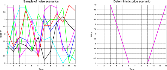
Figure 2: Samples of the noise process $\mathbf{W}$ (left) and price scenario $p$ (right)

4.2 Resolution of the problem with dualized expectation constraint

The method used here to solve Problem (17) is based on the duality argument described in §3.3. The probability constraint (17f) is dualized with associated multiplier $\lambda$, which leads, in the cost function (17a), to an added term of the form:

$$\lambda\>{{\mathbb{E}}}\big{[}{\pi-\mathbf{1}_{\mathbb{R}^{+}}(\boldsymbol{X^{\textstyle\text{\unboldmath$\scriptstyle$}}_{\textstyle\text{\unboldmath$\scriptstyle T$}}}-\ell)}\big{]}\;.$$

Instead of guessing the parameter value $\lambda$ leading to the constraint level $\ell$, we solve the dual problem

$$\max_{\lambda\geq 0}\;\;\varphi(\lambda)\;,$$ (19)

with

$$\varphi(\lambda)\;=\; \min_{\boldsymbol{U^{\textstyle\text{\unboldmath$\scriptstyle$}}_{\textstyle\text{\unboldmath$\scriptstyle$}}},\boldsymbol{X^{\textstyle\text{\unboldmath$\scriptstyle$}}_{\textstyle\text{\unboldmath$\scriptstyle$}}}}{{\mathbb{E}}}\bigg{[}{\sum_{t=0}^{T{-}1}-p_{t}\cdot\widetilde{\boldsymbol{U^{\textstyle\text{\unboldmath$\scriptstyle$}}_{\textstyle\text{\unboldmath$\scriptstyle$}}}}_{t}\;-\;\lambda\cdot\mathbf{1}_{\mathbb{R}^{+}}(\boldsymbol{X^{\textstyle\text{\unboldmath$\scriptstyle$}}_{\textstyle\text{\unboldmath$\scriptstyle T$}}}-\ell)}\bigg{]}\;,$$ (20a)

under constraints (17b)–(17c)–(17d)–(17e). (20b)

The Uzawa algorithm consists in maximizing the dual function $\varphi$ using a projected gradient algorithm. At iteration $k$ of the algorithm, knowing the value $\lambda^{(k)}$ of the multiplier, we perform the three following steps.

• Compute $\varphi(\lambda^{(k)})$, that is, solve the minimization problem (20) with $\lambda=\lambda^{(k)}$; this minimization is performed using dynamic programming (1-dimensional state variable), hence furnishing optimal feedbacks $\phi^{(k+1)}_{t}$ and optimal state variables $\boldsymbol{X^{\textstyle\text{\unboldmath$\scriptstyle(k+1)$}}_{\textstyle\text{\unboldmath$\scriptstyle t$}}}$.

• Compute the probability distribution of the random variable $\boldsymbol{X^{\textstyle\text{\unboldmath$\scriptstyle(k+1)$}}_{\textstyle\text{\unboldmath$\scriptstyle T$}}}$ by integrating the dynamics (17b)-(17c) using the optimal feedbacks $\phi^{(k+1)}_{t}$, and then compute the value of the constraint ${{\mathbb{P}}}[{\boldsymbol{X^{\textstyle\text{\unboldmath$\scriptstyle(k+1)$}}_{\textstyle\text{\unboldmath$\scriptstyle T$}}}\geq\ell}]$ .

• Update the multiplier $\lambda$ by a projected gradient step:

  $$\lambda^{(k+1)}=\mathrm{proj}_{\mathbb{R}^{+}}\left(\lambda^{(k)}+\rho\big{(}{\pi-{{\mathbb{P}}}[{\boldsymbol{X^{\textstyle\text{\unboldmath$\scriptstyle(k+1)$}}_{\textstyle\text{\unboldmath$\scriptstyle T$}}}\geq\ell}]}\big{)}\right)\;.$$

For the problem under consideration, and despite the potential nonconvexity induced by the final probability constraint (17f), the Uzawa algorithm converges in about 10 iterations, leading to an optimal multiplier value $\lambda^{\sharp}=62.405$. Once the algorithm has converged, we obtain the optimal feedback sequence $\{{\phi_{t}^{\sharp}}\}_{t=0,\dots,T{-}1}$ by solving Problem (20) by dynamic programming with $\lambda=\lambda^{\sharp}$. Then, we simulate the dynamics of the dam along some noise trajectories using these optimal feedbacks $\phi_{t}^{\sharp}$. The results given in Table 1 are obtained by simulating 10,000 noise trajectories, and illustrates the adequacy between optimization and simulation.

Uzawa optimization	Monte Carlo simulation
Bellman value at $t=0$: $-188.90$	Monte Carlo cost: $-188.94$
Required probability: $0.900$	Estimated probability: $0.903$

Table 1: Optimization and simulation for the duality method

On Figure 3, we represent the dam water level and control trajectories over $[0,T]$ obtained by simulating with the optimal feedbacks $\phi_{t}^{\sharp}$ along the noise trajectories depicted on Figure 2. We observe that the optimization “gives up” for certain trajectories (the lowest one to the left of Figure 3) to reach the final level $\ell$ appearing in the constraint in probability: we turbine as much water as possible, leaving the state evolve towards the minimum level $\underline{x}$. This observation is conform to the expected behavior of an optimization problem with a probability constraint.

Figure 3: Optimal state $\mathbf{X}$ and control $\mathbf{U}$ trajectories over $[0,T]$ obtained by the duality method

Finally, we can use the optimal feedbacks $\phi^{\sharp}_{t}$ to simulate the dam starting at any initial time $t_{i}>0$ from any given initial state $x_{t_{i}}$. For example starting at time $t_{i}=3$ from the initial state $x_{t_{i}}=5$ and simulating the optimal feedbacks $\phi^{\sharp}_{t}$ along 10,000 scenarios leads to the results given in Table 2. As expected, the final constraint level reached in this last simulation is not equal to the required level $\pi=0.9$, which illustrates that time consistency does not hold true for the problem formulation with dualized constraint.

Monte Carlo simulation
Monte Carlo cost: $-92.04$
Estimated probability: $0.833$

Table 2: Simulation for the duality method starting from $t_{i}=3$ and $x_{t_{i}}=5$

4.3 Resolution by extended dynamic programming

We now use the equivalent formulation of Problem (17) incorporating an additional state process $\boldsymbol{Z^{\textstyle\text{\unboldmath$\scriptstyle$}}_{\textstyle\text{\unboldmath$\scriptstyle$}}}=(\boldsymbol{Z^{\textstyle\text{\unboldmath$\scriptstyle$}}_{\textstyle\text{\unboldmath$\scriptstyle 0$}}},\ldots,\boldsymbol{Z^{\textstyle\text{\unboldmath$\scriptstyle$}}_{\textstyle\text{\unboldmath$\scriptstyle T$}}})$, an additional control process $\boldsymbol{V^{\textstyle\text{\unboldmath$\scriptstyle$}}_{\textstyle\text{\unboldmath$\scriptstyle$}}}=(\boldsymbol{V^{\textstyle\text{\unboldmath$\scriptstyle$}}_{\textstyle\text{\unboldmath$\scriptstyle 0$}}},\ldots,\boldsymbol{V^{\textstyle\text{\unboldmath$\scriptstyle$}}_{\textstyle\text{\unboldmath$\scriptstyle T{-}1$}}})$ and an almost sure contraint on the final state. As it has been explained in §3.2, the expression of the new dynamics, here 1-dimensional, is

$$\boldsymbol{Z^{\textstyle\text{\unboldmath$\scriptstyle$}}_{\textstyle\text{\unboldmath$\scriptstyle 0$}}}=z_{0}\;,\enspace\quad\;\boldsymbol{Z^{\textstyle\text{\unboldmath$\scriptstyle$}}_{\textstyle\text{\unboldmath$\scriptstyle t+1$}}}=\boldsymbol{Z^{\textstyle\text{\unboldmath$\scriptstyle$}}_{\textstyle\text{\unboldmath$\scriptstyle t$}}}+\boldsymbol{V^{\textstyle\text{\unboldmath$\scriptstyle$}}_{\textstyle\text{\unboldmath$\scriptstyle t$}}}\;,$$

and the form of the final constraint is

$$-\mathbf{1}_{\mathbb{R}^{+}}(\boldsymbol{X^{\textstyle\text{\unboldmath$\scriptstyle$}}_{\textstyle\text{\unboldmath$\scriptstyle T$}}}-\ell)-\boldsymbol{Z^{\textstyle\text{\unboldmath$\scriptstyle$}}_{\textstyle\text{\unboldmath$\scriptstyle T$}}}\leq 0\;.$$

The equivalent problem for the case study under consideration is

$$\min_{\boldsymbol{U^{\textstyle\text{\unboldmath$\scriptstyle$}}_{\textstyle\text{\unboldmath$\scriptstyle$}}},\boldsymbol{V^{\textstyle\text{\unboldmath$\scriptstyle$}}_{\textstyle\text{\unboldmath$\scriptstyle$}}},\boldsymbol{X^{\textstyle\text{\unboldmath$\scriptstyle$}}_{\textstyle\text{\unboldmath$\scriptstyle$}}},\boldsymbol{Z^{\textstyle\text{\unboldmath$\scriptstyle$}}_{\textstyle\text{\unboldmath$\scriptstyle$}}}}\;\; {{\mathbb{E}}}\bigg{[}{\sum_{t=0}^{T{-}1}-p_{t}\cdot\min\big{\{}{\boldsymbol{U^{\textstyle\text{\unboldmath$\scriptstyle$}}_{\textstyle\text{\unboldmath$\scriptstyle t$}}},\boldsymbol{X^{\textstyle\text{\unboldmath$\scriptstyle$}}_{\textstyle\text{\unboldmath$\scriptstyle t$}}}+\boldsymbol{W^{\textstyle\text{\unboldmath$\scriptstyle$}}_{\textstyle\text{\unboldmath$\scriptstyle t+1$}}}-\underline{x}}\big{\}}}\bigg{]}\;,$$ (21a)

s.t. $$\boldsymbol{X^{\textstyle\text{\unboldmath$\scriptstyle$}}_{\textstyle\text{\unboldmath$\scriptstyle 0$}}}=x_{0}\;,\enspace\;\boldsymbol{X^{\textstyle\text{\unboldmath$\scriptstyle$}}_{\textstyle\text{\unboldmath$\scriptstyle t+1$}}}=\min\big{\{}{\overline{x},\max\{{\underline{x},\boldsymbol{X^{\textstyle\text{\unboldmath$\scriptstyle$}}_{\textstyle\text{\unboldmath$\scriptstyle t$}}}-\boldsymbol{U^{\textstyle\text{\unboldmath$\scriptstyle$}}_{\textstyle\text{\unboldmath$\scriptstyle t$}}}+\boldsymbol{W^{\textstyle\text{\unboldmath$\scriptstyle$}}_{\textstyle\text{\unboldmath$\scriptstyle t+1$}}}}\}}\big{\}}\;,$$ (21b)

$$\boldsymbol{Z^{\textstyle\text{\unboldmath$\scriptstyle$}}_{\textstyle\text{\unboldmath$\scriptstyle 0$}}}=z_{0}\;,\enspace\;\;\boldsymbol{Z^{\textstyle\text{\unboldmath$\scriptstyle$}}_{\textstyle\text{\unboldmath$\scriptstyle t+1$}}}=\boldsymbol{Z^{\textstyle\text{\unboldmath$\scriptstyle$}}_{\textstyle\text{\unboldmath$\scriptstyle t$}}}+\boldsymbol{V^{\textstyle\text{\unboldmath$\scriptstyle$}}_{\textstyle\text{\unboldmath$\scriptstyle t$}}}\;,$$ (21c)

$$\underline{u}\leq\boldsymbol{U^{\textstyle\text{\unboldmath$\scriptstyle$}}_{\textstyle\text{\unboldmath$\scriptstyle t$}}}\leq\overline{u}\;,$$ (21d)

$$\sigma\big{(}{\boldsymbol{U^{\textstyle\text{\unboldmath$\scriptstyle$}}_{\textstyle\text{\unboldmath$\scriptstyle t$}}}}\big{)}\subset\sigma\big{(}{\boldsymbol{W^{\textstyle\text{\unboldmath$\scriptstyle$}}_{\textstyle\text{\unboldmath$\scriptstyle 1$}}},\dots,\boldsymbol{W^{\textstyle\text{\unboldmath$\scriptstyle$}}_{\textstyle\text{\unboldmath$\scriptstyle t$}}}}\big{)}\;,$$ (21e)

$$\sigma\big{(}{\boldsymbol{V^{\textstyle\text{\unboldmath$\scriptstyle$}}_{\textstyle\text{\unboldmath$\scriptstyle t$}}}}\big{)}\subset\sigma\big{(}{\boldsymbol{W^{\textstyle\text{\unboldmath$\scriptstyle$}}_{\textstyle\text{\unboldmath$\scriptstyle 1$}}},\dots,\boldsymbol{W^{\textstyle\text{\unboldmath$\scriptstyle$}}_{\textstyle\text{\unboldmath$\scriptstyle t+1$}}}}\big{)}\;,$$ (21f)

$${\mathbb{E}}\Big{[}{\boldsymbol{V^{\textstyle\text{\unboldmath$\scriptstyle$}}_{\textstyle\text{\unboldmath$\scriptstyle t$}}}\,\Big{|}\,\sigma\big{(}{\boldsymbol{W^{\textstyle\text{\unboldmath$\scriptstyle$}}_{\textstyle\text{\unboldmath$\scriptstyle 1$}}},\dots,\boldsymbol{W^{\textstyle\text{\unboldmath$\scriptstyle$}}_{\textstyle\text{\unboldmath$\scriptstyle t$}}}}\big{)}}\Big{]}=0\;,$$ (21g)

$$\mathbf{1}_{\mathbb{R}^{+}}(\boldsymbol{X^{\textstyle\text{\unboldmath$\scriptstyle$}}_{\textstyle\text{\unboldmath$\scriptstyle T$}}}-\ell)+\boldsymbol{Z^{\textstyle\text{\unboldmath$\scriptstyle$}}_{\textstyle\text{\unboldmath$\scriptstyle T$}}}\geq 0\;.$$ (21h)

From Proposition 5, we have that Problems (17) and (21) are equivalent under the condition

$$z_{0}=-\pi\;.$$

Moreover, the special form (21h) of the final constraint makes it possible to bound the variables $\boldsymbol{V^{\textstyle\text{\unboldmath$\scriptstyle$}}_{\textstyle\text{\unboldmath$\scriptstyle t$}}}$ and $\boldsymbol{~{}Z^{\textstyle\text{\unboldmath$\scriptstyle$}}_{\textstyle\text{\unboldmath$\scriptstyle t$}}}$. Indeed, from the proof of Proposition 5, we deduce from the expression (12a) of the optimal control $\boldsymbol{V^{\textstyle\text{\unboldmath$\scriptstyle$}}_{\textstyle\text{\unboldmath$\scriptstyle t$}}}^{\sharp}$ with $g=\mathbf{1}_{\mathbb{R}^{+}}$ that it is sufficient to search for the control $\boldsymbol{V^{\textstyle\text{\unboldmath$\scriptstyle$}}_{\textstyle\text{\unboldmath$\scriptstyle t$}}}$ in $[-1,1]$. Moreover, the optimal state $\boldsymbol{Z^{\textstyle\text{\unboldmath$\scriptstyle$}}_{\textstyle\text{\unboldmath$\scriptstyle t$}}}^{\sharp}$ being obtained by a telescoping sum, it is sufficient to search for the state $\boldsymbol{Z^{\textstyle\text{\unboldmath$\scriptstyle$}}_{\textstyle\text{\unboldmath$\scriptstyle t$}}}$ in $[z_{0}-1,z_{0}+1]$. Problem (21) can be solved by dynamic programming with the extended state variable $(\boldsymbol{X^{\textstyle\text{\unboldmath$\scriptstyle$}}_{\textstyle\text{\unboldmath$\scriptstyle t$}}},\boldsymbol{Z^{\textstyle\text{\unboldmath$\scriptstyle$}}_{\textstyle\text{\unboldmath$\scriptstyle t$}}})$, which corresponds to a dynamic programming equation with a 2-dimensional state variable. Then, we simulate the dynamics of the dam — using the same 10,000 noise trajectories as those previously used to obtain Table 1 — with the optimal feedbacks given by dynamic programming with the extended state variable $(\boldsymbol{X^{\textstyle\text{\unboldmath$\scriptstyle$}}_{\textstyle\text{\unboldmath$\scriptstyle t$}}},\boldsymbol{Z^{\textstyle\text{\unboldmath$\scriptstyle$}}_{\textstyle\text{\unboldmath$\scriptstyle t$}}})$. The associated results are given in Table 3. We observe a good adequacy between optimization and simulation, and we observe that the costs are pretty much identical between Table 1 and Table 3.

Extended Dynamic Programming	Monte Carlo Simulation
Bellman value at $t=0$: $-188.67$	Monte Carlo cost: $-187.47$
Initial state $z_{0}$: $-0.900$	Estimated probability: $0.896$

Table 3: Optimization and simulation for the extended dynamic programming method

Some simulation trajectories are represented on Figure 4 and Figure 5. Figure 4 gives the same information (dam water level and control trajectories over $[0,T]$) as the one presented for the duality based algorithm in §4.2, whereas Figure 5 depicts trajectories of the optimal state process $\boldsymbol{Z^{\textstyle\text{\unboldmath$\scriptstyle$}}_{\textstyle\text{\unboldmath$\scriptstyle$}}}$ and the optimal control process $\boldsymbol{V^{\textstyle\text{\unboldmath$\scriptstyle$}}_{\textstyle\text{\unboldmath$\scriptstyle$}}}$. We observe that the results depicted on Figure 3 (duality method) and on Figure 4 (extended dynamic programming method) are very close (with tiny differences induced by numerical resolution), which illustrates the equivalence between Problem (17) and Problem (21).

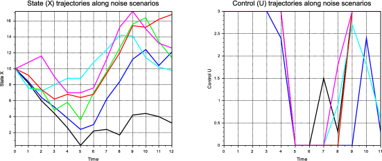
Figure 4: Optimal state $X$ and control $U$ trajectories over $[0,T]$ obtained by the extended dynamic programming method

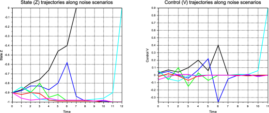
Figure 5: Optimal state $Z$ and control $V$ trajectories over $[0,T]$ obtained by the extended dynamic programming method

Finally, we can use the optimal feedbacks obtained when solving Problem (21) by dynamic programming to simulate the dam starting at any initial time $t_{i}>0$ from any given initial state $(x_{t_{i}},z_{t_{i}})$. For example starting at time $t_{i}=3$ from the initial state $(x_{t_{i}},z_{t_{i}})=(5,-0.9)$ — using the same values than those used in §4.2 — and simulating the optimal feedbacks along 10,000 scenarios leads to the results given in Table 4: the final probability level to be reached is by construction equal to $\pi=0.9$, and the Monte Carlo simulation induces a very similar level of probability, which numerically illustrates that the time consistency property is fulfilled. The associated simulation trajectories are represented on Figure 6, using the same noises trajectories as those that had been used to obtain Figure 3.

Extended Dynamic Programming	Monte Carlo Simulation
Bellman value at $t=3$: $-87.78$	Monte Carlo cost: $-87.71$
Initial state $(x_{3},z_{3})$: $(5,-0.900)$	Estimated probability: $0.902$

Table 4: Optimization and simulation for the extended dynamic programming method

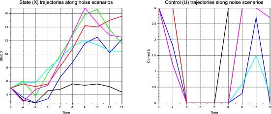
Figure 6: Optimal state $X$ and control $U$ trajectories over $[3,T]$ obtained by the extended dynamic programming method

5 Conclusion

In this paper, we have proposed a formal definition of time consistency for families of optimization problems, by introducing the notion of universal solution. With this, we have shown that — for the class of problems where risk is modeled in the form of constraints in probability or in expectation — the property of time consistency depends on the notion of state that one chooses, which must be suited to the problem studied. In particular, we have shown that, even if the “right” notion of state for the class of multistage stochastic optimization problems with a final expectation state constraint was of infinite dimension (the conditional probability distribution of the state), it is possible to display a state of finite dimension, so that solving the problem by dynamic programming becomes conceivable again.

Acknowledgements:

This paper builds upon results obtained by Pierre Girardeau during his PhD thesis [9], supervised by the three authors.

Appendix A An extension of Everett’s theorem

A result due to Everett (see [8]) links the solution of an optimization problem under constraint and the one of the related dualized optimization problem. We give here a slight extension, which relaxes an assumption of Everett’s theorem.

Let $\mathbb{U}$ be a set and let $U^{\mathrm{ad}}$ be a subset of $\mathbb{U}$. Let $\Theta:\mathbb{U}\to\mathbb{R}^{m}$ be a (mulivalued) function. We deal with the following optimization problem

$$J^{\sharp}=\min_{u\in U^{\mathrm{ad}}}J(u)\quad\text{s.t.}\quad\Theta(u)-b\leq 0\in\mathbb{R}^{m}\;,$$ (22)

hence subject to a finite number $m$ of inequality constraints.

Theorem 9

Let $\lambda\in\mathbb{R}^{m}_{+}$ be given. We consider $\overline{u}^{\lambda}$, solution of the optimization problem

$$\min_{u\in U^{\mathrm{ad}}}J(u)+\big{\langle}{\lambda,\,\Theta(u)}\big{\rangle}\;,$$ (23)

and we set $\overline{b}^{\lambda}=\Theta(\overline{u}^{\lambda})$. We introduce the set $B^{\lambda}\subset\mathbb{R}^{m}$ defined by

$$B^{\lambda}=\big{\{}{b\in\mathbb{R}^{m}\,\big{|}\,b_{i}=\overline{b}^{\lambda}_{i}\text{ if }\lambda_{i}>0\;\text{ and }\;b_{i}\geq\overline{b}^{\lambda}_{i}\text{ if }\lambda_{i}=0\;,\enspace\forall i=1,\dots,m}\big{\}}\;.$$ (24)

Then, a solution $\overline{u}^{\lambda}$ of Problem (23) is a solution of Problem (22) for any $b\in B^{\lambda}$.

Proof. Let $\overline{u}^{\lambda}$ be a solution of Problem (23) and let $b\in B^{\lambda}$. We have

$$J(\overline{u}^{\lambda}) =\min_{u\in U^{\mathrm{ad}}}J(u)+\big{\langle}{\lambda,\,\Theta(u)-\Theta(\overline{u}^{\lambda})}\big{\rangle}\;, \overline{u}^{\lambda}$$ (by definition of )

$$=\min_{u\in U^{\mathrm{ad}}}J(u)+\big{\langle}{\lambda,\,\Theta(u)-\overline{b}^{\lambda}}\big{\rangle}\;, \overline{b}^{\lambda}=\Theta(\overline{u}^{\lambda})$$ (by definition of )

$$=\min_{u\in U^{\mathrm{ad}}}J(u)+\big{\langle}{\lambda,\,\Theta(u)-b}\big{\rangle}\;, B^{\lambda}$$ (by definition of  in (24))

$$\leq\sup_{\mu\geq 0}\min_{u\in U^{\mathrm{ad}}}J(u)+\big{\langle}{\mu,\,\Theta(u)-b}\big{\rangle}\;, \lambda\geq 0$$ (as )

$$\leq\inf_{u\in U^{\mathrm{ad}}}\sup_{\mu\geq 0}J(u)+\big{\langle}{\mu,\,\Theta(u)-b}\big{\rangle}\;,$$ (by weak duality)

$$=J^{\sharp}\;.$$ (by (22))

Since $\overline{u}^{\lambda}$ is such that $\Theta(\overline{u}^{\lambda})=\overline{b}^{\lambda}\leq b$ by definition of the set $B^{\lambda}$ in (24), we deduce that $\overline{u}^{\lambda}$ is admissible for Problem (22), and hence is an optimal solution of this problem. $\Box$

Appendix B Dynamic programming for the optimization problem involving martingale-type constraints

We prove in §B.2 that Problem (9) can be solved by dynamic programming under the additional assumption that, for any time $t$ in $\llbracket 0,T\rrbracket$, the random variable $\boldsymbol{W^{\textstyle\text{\unboldmath$\scriptstyle$}}_{\textstyle\text{\unboldmath$\scriptstyle t$}}}$ can take only a finite number of values. The proof is based on a so-called interchange (between minimization and integration) lemma given in §B.1.

B.1 An interchange Lemma

Lemma 10

Let $\mathbb{Y}$, $\mathbb{U}$, $\mathbb{V}$, $\mathbb{W}^{\prime}$ and $\mathbb{W}^{\prime\prime}$ be measurable spaces, and let $\varphi:\mathbb{Y}\times\mathbb{U}\times\mathbb{V}\times\mathbb{W}^{\prime\prime}\to{\mathbb{R}}_{+}\cup\{{+\infty}\}$ be a measurable extended real function. Let $(\Omega,{\cal F},\mathbb{P})$ be a probability space. Given three random variables $\boldsymbol{Y^{\textstyle\text{\unboldmath$\scriptstyle$}}_{\textstyle\text{\unboldmath$\scriptstyle$}}}$, $\boldsymbol{W^{\textstyle\text{\unboldmath$\scriptstyle$}}_{\textstyle\text{\unboldmath$\scriptstyle$}}}^{\prime}$ and $\boldsymbol{W^{\textstyle\text{\unboldmath$\scriptstyle$}}_{\textstyle\text{\unboldmath$\scriptstyle$}}}^{\prime\prime}$ taking values in $\mathbb{Y}$, $\mathbb{W}^{\prime}$ and $\mathbb{W}^{\prime\prime}$ respectively, we consider the optimization problem ${\cal P}$ defined by

$${\cal V}_{\cal P}[{\boldsymbol{Y^{\textstyle\text{\unboldmath$\scriptstyle$}}_{\textstyle\text{\unboldmath$\scriptstyle$}}}}]=\inf_{(\boldsymbol{U^{\textstyle\text{\unboldmath$\scriptstyle$}}_{\textstyle\text{\unboldmath$\scriptstyle$}}},\boldsymbol{V^{\textstyle\text{\unboldmath$\scriptstyle$}}_{\textstyle\text{\unboldmath$\scriptstyle$}}})}\; {{\mathbb{E}}}\big{[}{\varphi(\boldsymbol{Y^{\textstyle\text{\unboldmath$\scriptstyle$}}_{\textstyle\text{\unboldmath$\scriptstyle$}}},\boldsymbol{U^{\textstyle\text{\unboldmath$\scriptstyle$}}_{\textstyle\text{\unboldmath$\scriptstyle$}}},\boldsymbol{V^{\textstyle\text{\unboldmath$\scriptstyle$}}_{\textstyle\text{\unboldmath$\scriptstyle$}}},\boldsymbol{W^{\textstyle\text{\unboldmath$\scriptstyle$}}_{\textstyle\text{\unboldmath$\scriptstyle$}}}^{\prime\prime})}\big{]}$$ (25a)

$$\text{s.t.}\quad\sigma({\boldsymbol{U^{\textstyle\text{\unboldmath$\scriptstyle$}}_{\textstyle\text{\unboldmath$\scriptstyle$}}}})\subset\sigma({\boldsymbol{W^{\textstyle\text{\unboldmath$\scriptstyle$}}_{\textstyle\text{\unboldmath$\scriptstyle$}}}^{\prime}})\;,\enspace\sigma({\boldsymbol{V^{\textstyle\text{\unboldmath$\scriptstyle$}}_{\textstyle\text{\unboldmath$\scriptstyle$}}}})\subset\sigma({\boldsymbol{W^{\textstyle\text{\unboldmath$\scriptstyle$}}_{\textstyle\text{\unboldmath$\scriptstyle$}}}^{\prime},\boldsymbol{W^{\textstyle\text{\unboldmath$\scriptstyle$}}_{\textstyle\text{\unboldmath$\scriptstyle$}}}^{\prime\prime}})\;,$$ (25b)

$$\hphantom{\text{s.t.}\quad}\boldsymbol{V^{\textstyle\text{\unboldmath$\scriptstyle$}}_{\textstyle\text{\unboldmath$\scriptstyle$}}}\text{ is integrable and }{\mathbb{E}}\big{[}{\boldsymbol{V^{\textstyle\text{\unboldmath$\scriptstyle$}}_{\textstyle\text{\unboldmath$\scriptstyle$}}}\,\big{|}\,\sigma({\boldsymbol{W^{\textstyle\text{\unboldmath$\scriptstyle$}}_{\textstyle\text{\unboldmath$\scriptstyle$}}}^{\prime}})}\big{]}=0\;,$$ (25c)

where the minimization is done over couples of random variables $\boldsymbol{U^{\textstyle\text{\unboldmath$\scriptstyle$}}_{\textstyle\text{\unboldmath$\scriptstyle$}}}:\Omega\to\mathbb{U}$ and $\boldsymbol{V^{\textstyle\text{\unboldmath$\scriptstyle$}}_{\textstyle\text{\unboldmath$\scriptstyle$}}}:\Omega\to\mathbb{V}$.

We define the function $\psi:\mathbb{Y}\to{\mathbb{R}}_{+}\cup\{{+\infty}\}$ by

$$\psi:\mathbb{Y}\ni y\mapsto \inf_{{(u,\boldsymbol{V^{\textstyle\text{\unboldmath$\scriptstyle$}}_{\textstyle\text{\unboldmath$\scriptstyle$}}})}}{{\mathbb{E}}}\big{[}{\varphi(y,u,\boldsymbol{V^{\textstyle\text{\unboldmath$\scriptstyle$}}_{\textstyle\text{\unboldmath$\scriptstyle$}}},\boldsymbol{W^{\textstyle\text{\unboldmath$\scriptstyle$}}_{\textstyle\text{\unboldmath$\scriptstyle$}}}^{\prime\prime})}\big{]}$$ (26)

$$\quad\text{s.t.}\quad\sigma({\boldsymbol{V^{\textstyle\text{\unboldmath$\scriptstyle$}}_{\textstyle\text{\unboldmath$\scriptstyle$}}}})\subset\sigma({\boldsymbol{W^{\textstyle\text{\unboldmath$\scriptstyle$}}_{\textstyle\text{\unboldmath$\scriptstyle$}}}^{\prime\prime}})\;,$$

$$\hphantom{\quad\text{s.t.}\quad}\boldsymbol{V^{\textstyle\text{\unboldmath$\scriptstyle$}}_{\textstyle\text{\unboldmath$\scriptstyle$}}}\text{ is integrable and }{{\mathbb{E}}}\big{[}{\boldsymbol{V^{\textstyle\text{\unboldmath$\scriptstyle$}}_{\textstyle\text{\unboldmath$\scriptstyle$}}}}\big{]}=0\;.$$

where the minimization is done over variables $u\in\mathbb{U}$ and random variables $\boldsymbol{V^{\textstyle\text{\unboldmath$\scriptstyle$}}_{\textstyle\text{\unboldmath$\scriptstyle$}}}:\Omega\to\mathbb{V}$.

We suppose that the two random variables $\boldsymbol{W^{\textstyle\text{\unboldmath$\scriptstyle$}}_{\textstyle\text{\unboldmath$\scriptstyle$}}}^{\prime}$ and $\boldsymbol{W^{\textstyle\text{\unboldmath$\scriptstyle$}}_{\textstyle\text{\unboldmath$\scriptstyle$}}}^{\prime\prime}$ are independent, that they each take a finite number of values, and that the random variable $\boldsymbol{Y^{\textstyle\text{\unboldmath$\scriptstyle$}}_{\textstyle\text{\unboldmath$\scriptstyle$}}}$ is $\sigma({\boldsymbol{W^{\textstyle\text{\unboldmath$\scriptstyle$}}_{\textstyle\text{\unboldmath$\scriptstyle$}}}^{\prime}})$-measurable, that is, $\sigma({\boldsymbol{Y^{\textstyle\text{\unboldmath$\scriptstyle$}}_{\textstyle\text{\unboldmath$\scriptstyle$}}}})\subset\sigma({\boldsymbol{W^{\textstyle\text{\unboldmath$\scriptstyle$}}_{\textstyle\text{\unboldmath$\scriptstyle$}}}^{\prime}})$. Then, the optimal value ${\cal V}_{\cal P}[{\boldsymbol{Y^{\textstyle\text{\unboldmath$\scriptstyle$}}_{\textstyle\text{\unboldmath$\scriptstyle$}}}}]$ of Problem ${\cal P}$ satisfies the following interchange formula

$${\cal V}_{\cal P}[{\boldsymbol{Y^{\textstyle\text{\unboldmath$\scriptstyle$}}_{\textstyle\text{\unboldmath$\scriptstyle$}}}}]={{\mathbb{E}}}\big{[}{\psi(\boldsymbol{Y^{\textstyle\text{\unboldmath$\scriptstyle$}}_{\textstyle\text{\unboldmath$\scriptstyle$}}})}\big{]}\;.$$ (27)

Proof. Letting $\{{w^{\prime}_{i}}\}_{i\in\llbracket 0,N^{\prime}\rrbracket}$ and $\{{w^{\prime\prime}_{i}}\}_{i\in\llbracket 0,N^{\prime\prime}\rrbracket}$ be the sets of values taken by, respectively, the random variables $\boldsymbol{W^{\textstyle\text{\unboldmath$\scriptstyle$}}_{\textstyle\text{\unboldmath$\scriptstyle$}}}^{\prime}$ and $\boldsymbol{W^{\textstyle\text{\unboldmath$\scriptstyle$}}_{\textstyle\text{\unboldmath$\scriptstyle$}}}^{\prime\prime}$, we denote

$$\boldsymbol{W^{\textstyle\text{\unboldmath$\scriptstyle$}}_{\textstyle\text{\unboldmath$\scriptstyle$}}}^{\prime}:\Omega\to\{{w^{\prime}_{i}}\}_{i\in\llbracket 0,N^{\prime}\rrbracket} \quad\text{with}\quad{{\mathbb{P}}}\big{[}{\{{\boldsymbol{W^{\textstyle\text{\unboldmath$\scriptstyle$}}_{\textstyle\text{\unboldmath$\scriptstyle$}}}=w^{\prime}_{i}}\}}\big{]}=\pi^{\prime}_{i}\;,\enspace\forall i\in\llbracket 0,N^{\prime}\rrbracket\;,$$ (28)

$$\boldsymbol{W^{\textstyle\text{\unboldmath$\scriptstyle$}}_{\textstyle\text{\unboldmath$\scriptstyle$}}}^{\prime\prime}:\Omega\to\{{w^{\prime\prime}_{i}}\}_{i\in\llbracket 0,N^{\prime\prime}\rrbracket} \quad\text{with}\quad{{\mathbb{P}}}\big{[}{\{{\boldsymbol{W^{\textstyle\text{\unboldmath$\scriptstyle$}}_{\textstyle\text{\unboldmath$\scriptstyle$}}}=w^{\prime\prime}_{i}}\}}\big{]}=\pi^{\prime\prime}_{i}\;,\enspace\forall i\in\llbracket 0,N^{\prime\prime}\rrbracket\;.$$ (29)

Now, since $\boldsymbol{Y^{\textstyle\text{\unboldmath$\scriptstyle$}}_{\textstyle\text{\unboldmath$\scriptstyle$}}}$ is a $\sigma(\boldsymbol{W^{\textstyle\text{\unboldmath$\scriptstyle$}}_{\textstyle\text{\unboldmath$\scriptstyle$}}}^{\prime})$-measurable random variable and from the measurability constraints on the random variables $\boldsymbol{U^{\textstyle\text{\unboldmath$\scriptstyle$}}_{\textstyle\text{\unboldmath$\scriptstyle$}}}$ and $\boldsymbol{V^{\textstyle\text{\unboldmath$\scriptstyle$}}_{\textstyle\text{\unboldmath$\scriptstyle$}}}$ in Equation (25b), we can represent these random variables as follows:

$$\boldsymbol{Y^{\textstyle\text{\unboldmath$\scriptstyle$}}_{\textstyle\text{\unboldmath$\scriptstyle$}}}=\sum_{i=0}^{N^{\prime}}y_{i}\mathbf{1}_{w^{\prime}_{i}}(\boldsymbol{W^{\textstyle\text{\unboldmath$\scriptstyle$}}_{\textstyle\text{\unboldmath$\scriptstyle$}}}^{\prime})\;,\enspace\boldsymbol{U^{\textstyle\text{\unboldmath$\scriptstyle$}}_{\textstyle\text{\unboldmath$\scriptstyle$}}}=\sum_{i=0}^{N^{\prime}}u_{i}\mathbf{1}_{w^{\prime}_{i}}(\boldsymbol{W^{\textstyle\text{\unboldmath$\scriptstyle$}}_{\textstyle\text{\unboldmath$\scriptstyle$}}}^{\prime})\;,\enspace\boldsymbol{V^{\textstyle\text{\unboldmath$\scriptstyle$}}_{\textstyle\text{\unboldmath$\scriptstyle$}}}=\sum_{i=0}^{N^{\prime}}\sum_{j=0}^{N^{\prime\prime}}v_{i,j}\mathbf{1}_{w^{\prime}_{i}}(\boldsymbol{W^{\textstyle\text{\unboldmath$\scriptstyle$}}_{\textstyle\text{\unboldmath$\scriptstyle$}}}^{\prime})\mathbf{1}_{w^{\prime\prime}_{j}}(\boldsymbol{W^{\textstyle\text{\unboldmath$\scriptstyle$}}_{\textstyle\text{\unboldmath$\scriptstyle$}}}^{\prime\prime})\;.$$ (30)

We have just expressed the fact that the set of $\sigma({\boldsymbol{W^{\textstyle\text{\unboldmath$\scriptstyle$}}_{\textstyle\text{\unboldmath$\scriptstyle$}}}})$-measurable random variables taking values in a set ${\mathbb{F}}$ is in bijection with the product space ${\mathbb{F}}^{N}$ if the random variable $\boldsymbol{W^{\textstyle\text{\unboldmath$\scriptstyle$}}_{\textstyle\text{\unboldmath$\scriptstyle$}}}$ takes $N$ different values.

We start the proof by using Equation (30) to establish the following equalities

$${\mathbb{E}}\big{[}{\varphi(\boldsymbol{Y^{\textstyle\text{\unboldmath$\scriptstyle$}}_{\textstyle\text{\unboldmath$\scriptstyle$}}},\boldsymbol{U^{\textstyle\text{\unboldmath$\scriptstyle$}}_{\textstyle\text{\unboldmath$\scriptstyle$}}},\boldsymbol{V^{\textstyle\text{\unboldmath$\scriptstyle$}}_{\textstyle\text{\unboldmath$\scriptstyle$}}},\boldsymbol{W^{\textstyle\text{\unboldmath$\scriptstyle$}}_{\textstyle\text{\unboldmath$\scriptstyle$}}}^{\prime\prime})\,\big{|}\,\boldsymbol{W^{\textstyle\text{\unboldmath$\scriptstyle$}}_{\textstyle\text{\unboldmath$\scriptstyle$}}}^{\prime}}\big{]} =\sum_{i=0}^{N^{\prime}}\Big{(}{\sum_{j=0}^{N^{\prime\prime}}\pi^{\prime\prime}_{j}\varphi\Big{(}{y_{i},u_{i},v_{i,j},w^{\prime\prime}_{j}}\Big{)}}\Big{)}\mathbf{1}_{w^{\prime}_{i}}(\boldsymbol{W^{\textstyle\text{\unboldmath$\scriptstyle$}}_{\textstyle\text{\unboldmath$\scriptstyle$}}}^{\prime})\;,$$ (31a)

$${{\mathbb{E}}}\big{[}{\varphi(\boldsymbol{Y^{\textstyle\text{\unboldmath$\scriptstyle$}}_{\textstyle\text{\unboldmath$\scriptstyle$}}},\boldsymbol{U^{\textstyle\text{\unboldmath$\scriptstyle$}}_{\textstyle\text{\unboldmath$\scriptstyle$}}},\boldsymbol{V^{\textstyle\text{\unboldmath$\scriptstyle$}}_{\textstyle\text{\unboldmath$\scriptstyle$}}},\boldsymbol{W^{\textstyle\text{\unboldmath$\scriptstyle$}}_{\textstyle\text{\unboldmath$\scriptstyle$}}}^{\prime\prime})}\big{]} =\sum_{i=0}^{N^{\prime}}\pi^{\prime}_{i}\Big{(}{\sum_{j=0}^{N^{\prime\prime}}\pi^{\prime\prime}_{j}\varphi\Big{(}{y_{i},u_{i},v_{i,j},w^{\prime\prime}_{j}}\Big{)}}\Big{)}\;,$$ (31b)

$${\mathbb{E}}\big{[}{\boldsymbol{V^{\textstyle\text{\unboldmath$\scriptstyle$}}_{\textstyle\text{\unboldmath$\scriptstyle$}}}\,\big{|}\,\boldsymbol{W^{\textstyle\text{\unboldmath$\scriptstyle$}}_{\textstyle\text{\unboldmath$\scriptstyle$}}}^{\prime}}\big{]} =\sum_{i=0}^{N^{\prime}}\bigg{(}{\sum_{j=0}^{N^{\prime\prime}}\pi^{\prime\prime}_{j}v_{i,j}}\bigg{)}\mathbf{1}_{w^{\prime}_{i}}(\boldsymbol{W^{\textstyle\text{\unboldmath$\scriptstyle$}}_{\textstyle\text{\unboldmath$\scriptstyle$}}}^{\prime})\;.$$ (31c)

All the manipulations below are easy to check, and are justified because all quantities take extended nonnegative values.

$\bullet$ For Equation (31a):

$${\mathbb{E}}\big{(} \varphi(\boldsymbol{Y^{\textstyle\text{\unboldmath$\scriptstyle$}}_{\textstyle\text{\unboldmath$\scriptstyle$}}},\boldsymbol{U^{\textstyle\text{\unboldmath$\scriptstyle$}}_{\textstyle\text{\unboldmath$\scriptstyle$}}},\boldsymbol{V^{\textstyle\text{\unboldmath$\scriptstyle$}}_{\textstyle\text{\unboldmath$\scriptstyle$}}},\boldsymbol{W^{\textstyle\text{\unboldmath$\scriptstyle$}}_{\textstyle\text{\unboldmath$\scriptstyle$}}}^{\prime\prime})\;\big{|}\;{\boldsymbol{W^{\textstyle\text{\unboldmath$\scriptstyle$}}_{\textstyle\text{\unboldmath$\scriptstyle$}}}^{\prime}}\big{)}$$

$$={\mathbb{E}}\bigg{[}{\varphi\Big{(}{\sum_{i=0}^{N^{\prime}}y_{i}\mathbf{1}_{w^{\prime}_{i}}(\boldsymbol{W^{\textstyle\text{\unboldmath$\scriptstyle$}}_{\textstyle\text{\unboldmath$\scriptstyle$}}}^{\prime}),\sum_{i=0}^{N^{\prime}}u_{i}\mathbf{1}_{w^{\prime}_{i}}(\boldsymbol{W^{\textstyle\text{\unboldmath$\scriptstyle$}}_{\textstyle\text{\unboldmath$\scriptstyle$}}}^{\prime}),\sum_{i=0}^{N^{\prime}}\sum_{j=0}^{N^{\prime\prime}}v_{i,j}\mathbf{1}_{w^{\prime}_{i}}(\boldsymbol{W^{\textstyle\text{\unboldmath$\scriptstyle$}}_{\textstyle\text{\unboldmath$\scriptstyle$}}}^{\prime})\mathbf{1}_{w^{\prime\prime}_{j}}(\boldsymbol{W^{\textstyle\text{\unboldmath$\scriptstyle$}}_{\textstyle\text{\unboldmath$\scriptstyle$}}}^{\prime\prime}),\boldsymbol{W^{\textstyle\text{\unboldmath$\scriptstyle$}}_{\textstyle\text{\unboldmath$\scriptstyle$}}}^{\prime\prime}}\Big{)}\,\bigg{|}\,\boldsymbol{W^{\textstyle\text{\unboldmath$\scriptstyle$}}_{\textstyle\text{\unboldmath$\scriptstyle$}}}^{\prime}}\bigg{]}$$ (by (30))

$$={\mathbb{E}}\bigg{[}{\sum_{i=0}^{N^{\prime}}\varphi\Big{(}{y_{i},u_{i},\sum_{j=0}^{N^{\prime\prime}}v_{i,j}\mathbf{1}_{w^{\prime\prime}_{j}}(\boldsymbol{W^{\textstyle\text{\unboldmath$\scriptstyle$}}_{\textstyle\text{\unboldmath$\scriptstyle$}}}^{\prime\prime}),\boldsymbol{W^{\textstyle\text{\unboldmath$\scriptstyle$}}_{\textstyle\text{\unboldmath$\scriptstyle$}}}^{\prime\prime}}\Big{)}\mathbf{1}_{w^{\prime}_{i}}(\boldsymbol{W^{\textstyle\text{\unboldmath$\scriptstyle$}}_{\textstyle\text{\unboldmath$\scriptstyle$}}}^{\prime})\,\bigg{|}\,\boldsymbol{W^{\textstyle\text{\unboldmath$\scriptstyle$}}_{\textstyle\text{\unboldmath$\scriptstyle$}}}^{\prime}}\bigg{]}$$

$$=\sum_{i=0}^{N^{\prime}}{\mathbb{E}}\bigg{[}{\varphi\Big{(}{y_{i},u_{i},\sum_{j=0}^{N^{\prime\prime}}v_{i,j}\mathbf{1}_{w^{\prime\prime}_{j}}(\boldsymbol{W^{\textstyle\text{\unboldmath$\scriptstyle$}}_{\textstyle\text{\unboldmath$\scriptstyle$}}}^{\prime\prime}),\boldsymbol{W^{\textstyle\text{\unboldmath$\scriptstyle$}}_{\textstyle\text{\unboldmath$\scriptstyle$}}}^{\prime\prime}}\Big{)}\,\bigg{|}\,\boldsymbol{W^{\textstyle\text{\unboldmath$\scriptstyle$}}_{\textstyle\text{\unboldmath$\scriptstyle$}}}^{\prime}}\bigg{]}\mathbf{1}_{w^{\prime}_{i}}(\boldsymbol{W^{\textstyle\text{\unboldmath$\scriptstyle$}}_{\textstyle\text{\unboldmath$\scriptstyle$}}}^{\prime})$$

$$=\sum_{i=0}^{N^{\prime}}{{\mathbb{E}}}\bigg{[}{\varphi\Big{(}{y_{i},u_{i},\sum_{j=0}^{N^{\prime\prime}}v_{i,j}\mathbf{1}_{w^{\prime\prime}_{j}}(\boldsymbol{W^{\textstyle\text{\unboldmath$\scriptstyle$}}_{\textstyle\text{\unboldmath$\scriptstyle$}}}^{\prime\prime}),\boldsymbol{W^{\textstyle\text{\unboldmath$\scriptstyle$}}_{\textstyle\text{\unboldmath$\scriptstyle$}}}^{\prime\prime}}\Big{)}}\bigg{]}\mathbf{1}_{w^{\prime}_{i}}(\boldsymbol{W^{\textstyle\text{\unboldmath$\scriptstyle$}}_{\textstyle\text{\unboldmath$\scriptstyle$}}}^{\prime}) \boldsymbol{W^{\textstyle\text{\unboldmath$\scriptstyle$}}_{\textstyle\text{\unboldmath$\scriptstyle$}}}^{\prime} \boldsymbol{W^{\textstyle\text{\unboldmath$\scriptstyle$}}_{\textstyle\text{\unboldmath$\scriptstyle$}}}^{\prime\prime}$$ (as and are independent)

$$=\sum_{i=0}^{N^{\prime}}{{\mathbb{E}}}\bigg{[}{\sum_{j=0}^{N^{\prime\prime}}\varphi\Big{(}{y_{i},u_{i},v_{i,j},w^{\prime\prime}_{j}}\Big{)}\mathbf{1}_{w^{\prime\prime}_{j}}(\boldsymbol{W^{\textstyle\text{\unboldmath$\scriptstyle$}}_{\textstyle\text{\unboldmath$\scriptstyle$}}}^{\prime\prime})}\bigg{]}\mathbf{1}_{w^{\prime}_{i}}(\boldsymbol{W^{\textstyle\text{\unboldmath$\scriptstyle$}}_{\textstyle\text{\unboldmath$\scriptstyle$}}}^{\prime})$$

$$=\sum_{i=0}^{N^{\prime}}\Big{(}{\sum_{j=0}^{N^{\prime\prime}}\pi^{\prime\prime}_{j}\varphi\Big{(}{y_{i},u_{i},v_{i,j},w^{\prime\prime}_{j}}\Big{)}}\Big{)}\mathbf{1}_{w^{\prime}_{i}}(\boldsymbol{W^{\textstyle\text{\unboldmath$\scriptstyle$}}_{\textstyle\text{\unboldmath$\scriptstyle$}}}^{\prime})\;.$$ (by (29))

$\bullet$ For Equation (31b):

$${{\mathbb{E}}}\big{[}{\varphi(\boldsymbol{Y^{\textstyle\text{\unboldmath$\scriptstyle$}}_{\textstyle\text{\unboldmath$\scriptstyle$}}},\boldsymbol{U^{\textstyle\text{\unboldmath$\scriptstyle$}}_{\textstyle\text{\unboldmath$\scriptstyle$}}},\boldsymbol{V^{\textstyle\text{\unboldmath$\scriptstyle$}}_{\textstyle\text{\unboldmath$\scriptstyle$}}},\boldsymbol{W^{\textstyle\text{\unboldmath$\scriptstyle$}}_{\textstyle\text{\unboldmath$\scriptstyle$}}}^{\prime\prime})}\big{]} ={{\mathbb{E}}}\Big{[}{{\mathbb{E}}\big{[}{\varphi(\boldsymbol{Y^{\textstyle\text{\unboldmath$\scriptstyle$}}_{\textstyle\text{\unboldmath$\scriptstyle$}}},\boldsymbol{U^{\textstyle\text{\unboldmath$\scriptstyle$}}_{\textstyle\text{\unboldmath$\scriptstyle$}}},\boldsymbol{V^{\textstyle\text{\unboldmath$\scriptstyle$}}_{\textstyle\text{\unboldmath$\scriptstyle$}}},\boldsymbol{W^{\textstyle\text{\unboldmath$\scriptstyle$}}_{\textstyle\text{\unboldmath$\scriptstyle$}}}^{\prime\prime})\,\big{|}\,\boldsymbol{W^{\textstyle\text{\unboldmath$\scriptstyle$}}_{\textstyle\text{\unboldmath$\scriptstyle$}}}^{\prime}}\big{]}}\Big{]}$$

$$={{\mathbb{E}}}\Big{[}{\sum_{i=0}^{N^{\prime}}\Big{(}{\sum_{j=0}^{N^{\prime\prime}}\pi^{\prime\prime}_{j}\varphi\Big{(}{y_{i},u_{i},v_{i,j},w^{\prime\prime}_{j}}\Big{)}}\Big{)}\mathbf{1}_{w^{\prime}_{i}}(\boldsymbol{W^{\textstyle\text{\unboldmath$\scriptstyle$}}_{\textstyle\text{\unboldmath$\scriptstyle$}}}^{\prime})}\Big{]}$$ (by (31a))

$$=\sum_{i=0}^{N^{\prime}}\pi^{\prime}_{i}\Big{(}{\sum_{j=0}^{N^{\prime\prime}}\pi^{\prime\prime}_{j}\varphi\Big{(}{y_{i},u_{i},v_{i,j},w^{\prime\prime}_{j}}\Big{)}}\Big{)}\;.$$ (by (28))

$\bullet$ For Equation (31c):

$${\mathbb{E}}\big{[}{\boldsymbol{V^{\textstyle\text{\unboldmath$\scriptstyle$}}_{\textstyle\text{\unboldmath$\scriptstyle$}}}\,\big{|}\,\boldsymbol{W^{\textstyle\text{\unboldmath$\scriptstyle$}}_{\textstyle\text{\unboldmath$\scriptstyle$}}}^{\prime}}\big{]} ={\mathbb{E}}\bigg{[}{\sum_{i=0}^{N^{\prime}}\sum_{j=0}^{N^{\prime\prime}}v_{i,j}\mathbf{1}_{w^{\prime}_{i}}(\boldsymbol{W^{\textstyle\text{\unboldmath$\scriptstyle$}}_{\textstyle\text{\unboldmath$\scriptstyle$}}}^{\prime})\mathbf{1}_{w^{\prime\prime}_{j}}(\boldsymbol{W^{\textstyle\text{\unboldmath$\scriptstyle$}}_{\textstyle\text{\unboldmath$\scriptstyle$}}}^{\prime\prime})\,\bigg{|}\,\boldsymbol{W^{\textstyle\text{\unboldmath$\scriptstyle$}}_{\textstyle\text{\unboldmath$\scriptstyle$}}}^{\prime}}\bigg{]}$$ (by (30))

$$=\sum_{i=0}^{N^{\prime}}{\mathbb{E}}\bigg{[}{\sum_{j=0}^{N^{\prime\prime}}v_{i,j}\mathbf{1}_{w^{\prime\prime}_{j}}(\boldsymbol{W^{\textstyle\text{\unboldmath$\scriptstyle$}}_{\textstyle\text{\unboldmath$\scriptstyle$}}}^{\prime\prime})\,\bigg{|}\,\boldsymbol{W^{\textstyle\text{\unboldmath$\scriptstyle$}}_{\textstyle\text{\unboldmath$\scriptstyle$}}}^{\prime}}\bigg{]}\mathbf{1}_{w^{\prime}_{i}}(\boldsymbol{W^{\textstyle\text{\unboldmath$\scriptstyle$}}_{\textstyle\text{\unboldmath$\scriptstyle$}}}^{\prime})$$

$$=\sum_{i=0}^{N^{\prime}}{{\mathbb{E}}}\bigg{[}{\sum_{j=0}^{N^{\prime\prime}}v_{i,j}\mathbf{1}_{w^{\prime\prime}_{j}}(\boldsymbol{W^{\textstyle\text{\unboldmath$\scriptstyle$}}_{\textstyle\text{\unboldmath$\scriptstyle$}}}^{\prime\prime})}\bigg{]}\mathbf{1}_{w^{\prime}_{i}}(\boldsymbol{W^{\textstyle\text{\unboldmath$\scriptstyle$}}_{\textstyle\text{\unboldmath$\scriptstyle$}}}^{\prime}) \boldsymbol{W^{\textstyle\text{\unboldmath$\scriptstyle$}}_{\textstyle\text{\unboldmath$\scriptstyle$}}}^{\prime} \boldsymbol{W^{\textstyle\text{\unboldmath$\scriptstyle$}}_{\textstyle\text{\unboldmath$\scriptstyle$}}}^{\prime\prime}$$ (as and are independent)

$$=\sum_{i=0}^{N^{\prime}}\bigg{(}{\sum_{j=0}^{N^{\prime\prime}}\pi^{\prime\prime}_{j}v_{i,j}}\bigg{)}\mathbf{1}_{w^{\prime}_{i}}(\boldsymbol{W^{\textstyle\text{\unboldmath$\scriptstyle$}}_{\textstyle\text{\unboldmath$\scriptstyle$}}}^{\prime})\;.$$ (by (29))

Using Equations (30) and (31c), for any $\sigma({\boldsymbol{W^{\textstyle\text{\unboldmath$\scriptstyle$}}_{\textstyle\text{\unboldmath$\scriptstyle$}}}^{\prime\prime}})$-measurable random variable $\boldsymbol{V^{\textstyle\text{\unboldmath$\scriptstyle$}}_{\textstyle\text{\unboldmath$\scriptstyle$}}}$, we have the equivalence

$${\mathbb{E}}\big{[}{\boldsymbol{V^{\textstyle\text{\unboldmath$\scriptstyle$}}_{\textstyle\text{\unboldmath$\scriptstyle$}}}\,\big{|}\,\boldsymbol{W^{\textstyle\text{\unboldmath$\scriptstyle$}}_{\textstyle\text{\unboldmath$\scriptstyle$}}}^{\prime}}\big{]}=0\iff\sum_{j=0}^{N^{\prime\prime}}\pi^{\prime\prime}_{j}v_{i,j}=0\;,\enspace\;\forall i\in\llbracket 0,N^{\prime}\rrbracket\;.$$ (35)

Using again Equations (30) and (31), we obtain that the optimization Problem (25) is equivalent to the following optimization problem

$$\inf_{\begin{subarray}{c}\{{u_{i}}\}_{i\in\llbracket 0,N^{\prime}\rrbracket}\\ \{{v_{i,j}}\}_{i\in\llbracket 0,N^{\prime}\rrbracket,j\in\llbracket 0,N^{\prime\prime}\rrbracket}\end{subarray}} \sum_{i=0}^{N^{\prime}}\pi^{\prime}_{i}\Big{(}{\sum_{j=0}^{N^{\prime\prime}}\pi^{\prime\prime}_{j}\varphi({y_{i},u_{i},v_{i,j},w^{\prime\prime}_{i}})}\Big{)}$$ (36a)

$$\text{s.t.}\quad{\sum_{j=0}^{N^{\prime\prime}}\pi^{\prime\prime}_{j}v_{i,j}=0\;,\enspace\;\forall i\in\llbracket 0,N^{\prime}\rrbracket}\;.$$ (36b)

The optimization problem (36) trivially splits into a family $\{{{\cal P}_{i}}\}_{i\in\llbracket 0,N^{\prime}\rrbracket}$ of $N^{\prime}$ independent optimization problems, Problem ${\cal P}_{i}$ being defined by

$${\cal V}_{{\cal{\cal P}}_{i}}[{y_{i}}]= \inf_{(u_{i},\{{v_{i,j}}\}_{j\in\llbracket 0,N^{\prime\prime}\rrbracket})}{\sum_{j=0}^{N^{\prime\prime}}\pi^{\prime\prime}_{j}\varphi({y_{i},u_{i},v_{i,j},w^{\prime\prime}_{i}})}$$ (37a)

$$\text{s.t.}\quad\sum_{j=0}^{N^{\prime\prime}}\pi^{\prime\prime}_{j}v_{i,j}=0\;,\enspace$$ (37b)

and the value of Problem (36) is the weighted sum of the values of the family of problems $\{{{\cal P}_{i}}\}_{i\in\llbracket 0,N^{\prime}\rrbracket}$:

$${\cal V}_{\cal P}[{\boldsymbol{Y^{\textstyle\text{\unboldmath$\scriptstyle$}}_{\textstyle\text{\unboldmath$\scriptstyle$}}}}]=\sum_{i=0}^{N^{\prime}}\pi^{\prime}_{i}{\cal V}_{{\cal{\cal P}}_{i}}[{y_{i}}]\;.$$

We notice that ${\cal V}_{{\cal{\cal P}}_{i}}[{y_{i}}]$ in (37) is exactly $\psi({y_{i}})$ in (26), so that the above equation gives (27). $\Box$

B.2 Proof of Theorem 6

Proof. For any $\tau\in\llbracket 0,T\rrbracket$ we consider the minimization Problem ${\cal P}_{\tau}$ defined by

$$\min_{(\boldsymbol{U^{\textstyle\text{\unboldmath$\scriptstyle$}}_{\textstyle\text{\unboldmath$\scriptstyle$}}},\boldsymbol{V^{\textstyle\text{\unboldmath$\scriptstyle$}}_{\textstyle\text{\unboldmath$\scriptstyle$}}},\boldsymbol{X^{\textstyle\text{\unboldmath$\scriptstyle$}}_{\textstyle\text{\unboldmath$\scriptstyle$}}},\boldsymbol{Z^{\textstyle\text{\unboldmath$\scriptstyle$}}_{\textstyle\text{\unboldmath$\scriptstyle$}}})} {{\mathbb{E}}}\bigg{[}{\sum_{t=0}^{\tau{-}1}L_{t}(\boldsymbol{X^{\textstyle\text{\unboldmath$\scriptstyle$}}_{\textstyle\text{\unboldmath$\scriptstyle t$}}},\boldsymbol{U^{\textstyle\text{\unboldmath$\scriptstyle$}}_{\textstyle\text{\unboldmath$\scriptstyle t$}}},\boldsymbol{W^{\textstyle\text{\unboldmath$\scriptstyle$}}_{\textstyle\text{\unboldmath$\scriptstyle t+1$}}})+\mathscr{V}_{\tau}(\boldsymbol{X^{\textstyle\text{\unboldmath$\scriptstyle$}}_{\textstyle\text{\unboldmath$\scriptstyle\tau$}}},\boldsymbol{Z^{\textstyle\text{\unboldmath$\scriptstyle$}}_{\textstyle\text{\unboldmath$\scriptstyle\tau$}}})}\bigg{]}\;,$$ (38a)

$$\text{s.t.}\;\boldsymbol{X^{\textstyle\text{\unboldmath$\scriptstyle$}}_{\textstyle\text{\unboldmath$\scriptstyle 0$}}}=x_{0}\;,\enspace\boldsymbol{Z^{\textstyle\text{\unboldmath$\scriptstyle$}}_{\textstyle\text{\unboldmath$\scriptstyle 0$}}}=z_{0}\;,\enspace$$ (38b)

and, for all $$t\in\llbracket 0,\tau-1\rrbracket$$,

$$\hphantom{\text{and}\;\forall t}\boldsymbol{X^{\textstyle\text{\unboldmath$\scriptstyle$}}_{\textstyle\text{\unboldmath$\scriptstyle t+1$}}}=f_{t}(\boldsymbol{X^{\textstyle\text{\unboldmath$\scriptstyle$}}_{\textstyle\text{\unboldmath$\scriptstyle t$}}},\boldsymbol{U^{\textstyle\text{\unboldmath$\scriptstyle$}}_{\textstyle\text{\unboldmath$\scriptstyle t$}}},\boldsymbol{W^{\textstyle\text{\unboldmath$\scriptstyle$}}_{\textstyle\text{\unboldmath$\scriptstyle t+1$}}})\;,\enspace\boldsymbol{Z^{\textstyle\text{\unboldmath$\scriptstyle$}}_{\textstyle\text{\unboldmath$\scriptstyle t+1$}}}=\boldsymbol{Z^{\textstyle\text{\unboldmath$\scriptstyle$}}_{\textstyle\text{\unboldmath$\scriptstyle t$}}}+\boldsymbol{V^{\textstyle\text{\unboldmath$\scriptstyle$}}_{\textstyle\text{\unboldmath$\scriptstyle t$}}}\;,$$ (38c)

$$\hphantom{\text{and}\;\forall t}\sigma\big{(}{\boldsymbol{U^{\textstyle\text{\unboldmath$\scriptstyle$}}_{\textstyle\text{\unboldmath$\scriptstyle t$}}}}\big{)}\subset\sigma\big{(}{\boldsymbol{W^{\textstyle\text{\unboldmath$\scriptstyle$}}_{\textstyle\text{\unboldmath$\scriptstyle 1$}}},\dots,\boldsymbol{W^{\textstyle\text{\unboldmath$\scriptstyle$}}_{\textstyle\text{\unboldmath$\scriptstyle t$}}}}\big{)}\;,\enspace\sigma\big{(}{\boldsymbol{V^{\textstyle\text{\unboldmath$\scriptstyle$}}_{\textstyle\text{\unboldmath$\scriptstyle t$}}}}\big{)}\subset\sigma\big{(}{\boldsymbol{W^{\textstyle\text{\unboldmath$\scriptstyle$}}_{\textstyle\text{\unboldmath$\scriptstyle 1$}}},\dots,\boldsymbol{W^{\textstyle\text{\unboldmath$\scriptstyle$}}_{\textstyle\text{\unboldmath$\scriptstyle t+1$}}}}\big{)}\;,$$ (38d)

$$\hphantom{\text{and}\;\forall t}\text{$\boldsymbol{V^{\textstyle\text{\unboldmath$\scriptstyle$}}_{\textstyle\text{\unboldmath$\scriptstyle t$}}}$ is integrable and }\;{\mathbb{E}}\big{[}{\boldsymbol{V^{\textstyle\text{\unboldmath$\scriptstyle$}}_{\textstyle\text{\unboldmath$\scriptstyle t$}}}\,\big{|}\,{\boldsymbol{W^{\textstyle\text{\unboldmath$\scriptstyle$}}_{\textstyle\text{\unboldmath$\scriptstyle 1$}}},\dots,\boldsymbol{W^{\textstyle\text{\unboldmath$\scriptstyle$}}_{\textstyle\text{\unboldmath$\scriptstyle t$}}}}}\big{]}=0\;,$$ (38e)

where the sequence $$\big{\{}{\mathscr{V}_{\tau}}\big{\}}_{\tau\in\llbracket 0,T\rrbracket} \mathscr{V}_{\tau}:\mathbb{X}_{\tau}\times\mathbb{Z}_{\tau}\to{\mathbb{R}}_{+}\cup\{{+\infty}\} \Lambda_{\tau} ({\boldsymbol{U^{\textstyle\text{\unboldmath$\scriptstyle$}}_{\textstyle\text{\unboldmath$\scriptstyle t$}}},\boldsymbol{V^{\textstyle\text{\unboldmath$\scriptstyle$}}_{\textstyle\text{\unboldmath$\scriptstyle t$}}}})_{t\in\llbracket 0,\tau\rrbracket} ({\boldsymbol{X^{\textstyle\text{\unboldmath$\scriptstyle$}}_{\textstyle\text{\unboldmath$\scriptstyle t$}}},\boldsymbol{Z^{\textstyle\text{\unboldmath$\scriptstyle$}}_{\textstyle\text{\unboldmath$\scriptstyle t$}}}})_{t\in\llbracket 0,\tau+1\rrbracket} \mathcal{F}_{\tau} \sigma ({\boldsymbol{W^{\textstyle\text{\unboldmath$\scriptstyle$}}_{\textstyle\text{\unboldmath$\scriptstyle 1$}}},\ldots,\boldsymbol{W^{\textstyle\text{\unboldmath$\scriptstyle$}}_{\textstyle\text{\unboldmath$\scriptstyle\tau$}}}}) \tau\in\llbracket 1,T\rrbracket$$ of value functions, with , appearing in the cost function (38a) is given by the Bellman recursion (13). To simplify the notation, we denote by the set of random variables and satisfying the constraints (38b) – (38c) – (38d) – (38e). We recall that, by Equation (10), represents the -field generated by for all .

We are now going to prove, by backward induction, that the value of Problem (9) with $t_{0}=0$ is equal to the value of Problem ${\cal P}_{\tau}$ in (38) for any $\tau\in\llbracket 0,T\rrbracket$.

First, the value of Problem (9), with $t_{0}=0$, is equal to the value of Problem ${\cal P}_{\tau}$ in (38) for $\tau=T$. Indeed, the criterion (38a) in Problem (38), satisfies, for $\tau=T$,

$${{\mathbb{E}}}\bigg{[}{\sum_{t=0}^{T{-}1}L_{t}(\boldsymbol{X^{\textstyle\text{\unboldmath$\scriptstyle$}}_{\textstyle\text{\unboldmath$\scriptstyle t$}}},\boldsymbol{U^{\textstyle\text{\unboldmath$\scriptstyle$}}_{\textstyle\text{\unboldmath$\scriptstyle t$}}},\boldsymbol{W^{\textstyle\text{\unboldmath$\scriptstyle$}}_{\textstyle\text{\unboldmath$\scriptstyle t+1$}}})+\mathscr{V}_{T}(\boldsymbol{X^{\textstyle\text{\unboldmath$\scriptstyle$}}_{\textstyle\text{\unboldmath$\scriptstyle T$}}},\boldsymbol{Z^{\textstyle\text{\unboldmath$\scriptstyle$}}_{\textstyle\text{\unboldmath$\scriptstyle T$}}})}\bigg{]}$$

$$={{\mathbb{E}}}\bigg{[}{\sum_{t=0}^{T{-}1}L_{t}(\boldsymbol{X^{\textstyle\text{\unboldmath$\scriptstyle$}}_{\textstyle\text{\unboldmath$\scriptstyle t$}}},\boldsymbol{U^{\textstyle\text{\unboldmath$\scriptstyle$}}_{\textstyle\text{\unboldmath$\scriptstyle t$}}},\boldsymbol{W^{\textstyle\text{\unboldmath$\scriptstyle$}}_{\textstyle\text{\unboldmath$\scriptstyle t+1$}}})+\big{(}{K(x)+\chi_{{}_{\{{g(x)-z\leq 0}\}}}}\big{)}(\boldsymbol{X^{\textstyle\text{\unboldmath$\scriptstyle$}}_{\textstyle\text{\unboldmath$\scriptstyle T$}}},\boldsymbol{Z^{\textstyle\text{\unboldmath$\scriptstyle$}}_{\textstyle\text{\unboldmath$\scriptstyle T$}}})}\bigg{]} \mathscr{V}_{T}$$ (as  is defined by (13a))

$$={{\mathbb{E}}}\bigg{[}{\sum_{t=0}^{T{-}1}L_{t}(\boldsymbol{X^{\textstyle\text{\unboldmath$\scriptstyle$}}_{\textstyle\text{\unboldmath$\scriptstyle t$}}},\boldsymbol{U^{\textstyle\text{\unboldmath$\scriptstyle$}}_{\textstyle\text{\unboldmath$\scriptstyle t$}}},\boldsymbol{W^{\textstyle\text{\unboldmath$\scriptstyle$}}_{\textstyle\text{\unboldmath$\scriptstyle t+1$}}})+K(\boldsymbol{X^{\textstyle\text{\unboldmath$\scriptstyle$}}_{\textstyle\text{\unboldmath$\scriptstyle T$}}})}\bigg{]}\,\mbox{ under the almost sure final constraint}\,$$

$$\hphantom{{{\mathbb{E}}}\bigg{[}{\sum_{t=0}^{T{-}1}L_{t}(\boldsymbol{X^{\textstyle\text{\unboldmath$\scriptstyle$}}_{\textstyle\text{\unboldmath$\scriptstyle t$}}},\boldsymbol{U^{\textstyle\text{\unboldmath$\scriptstyle$}}_{\textstyle\text{\unboldmath$\scriptstyle t$}}},\boldsymbol{W^{\textstyle\text{\unboldmath$\scriptstyle$}}_{\textstyle\text{\unboldmath$\scriptstyle t+1$}}})+K(\boldsymbol{X^{\textstyle\text{\unboldmath$\scriptstyle$}}_{\textstyle\text{\unboldmath$\scriptstyle T$}}})}\bigg{]}\,\mbox{ under the}\,}g(\boldsymbol{X^{\textstyle\text{\unboldmath$\scriptstyle$}}_{\textstyle\text{\unboldmath$\scriptstyle T$}}})-\boldsymbol{Z^{\textstyle\text{\unboldmath$\scriptstyle$}}_{\textstyle\text{\unboldmath$\scriptstyle T$}}}\leq 0\;.$$

Thus, we obtain that Problem (38) for $\tau=T$ is the same as Problem (9) with $t_{0}=0$, the only difference being that the almost sure final constraint (9g) has been moved in the final cost in (38a).

Second, we prove by backward induction that the value of Problem (9) is equal to the value of Problem ${\cal P}_{\tau}$ for any $\tau\in\llbracket 0,T\rrbracket$. For this purpose, assuming that the value of Problem (9) is equal to the value of Problem ${\cal P}_{\tau+1}$, we prove that it is also equal to the value of Problem ${\cal P}_{\tau}$. We immediately get that

$$\min_{\big{(}{({\boldsymbol{U^{\textstyle\text{\unboldmath$\scriptstyle$}}_{\textstyle\text{\unboldmath$\scriptstyle t$}}},\boldsymbol{V^{\textstyle\text{\unboldmath$\scriptstyle$}}_{\textstyle\text{\unboldmath$\scriptstyle t$}}}})_{t\in\llbracket 0,\tau\rrbracket},({\boldsymbol{X^{\textstyle\text{\unboldmath$\scriptstyle$}}_{\textstyle\text{\unboldmath$\scriptstyle t$}}},\boldsymbol{Z^{\textstyle\text{\unboldmath$\scriptstyle$}}_{\textstyle\text{\unboldmath$\scriptstyle t$}}}})_{t\in\llbracket 0,\tau+1\rrbracket}}\big{)}\in\Lambda_{\tau}}{{\mathbb{E}}}\bigg{[}{\sum_{t=0}^{\tau}L_{t}(\boldsymbol{X^{\textstyle\text{\unboldmath$\scriptstyle$}}_{\textstyle\text{\unboldmath$\scriptstyle t$}}},\boldsymbol{U^{\textstyle\text{\unboldmath$\scriptstyle$}}_{\textstyle\text{\unboldmath$\scriptstyle t$}}},\boldsymbol{W^{\textstyle\text{\unboldmath$\scriptstyle$}}_{\textstyle\text{\unboldmath$\scriptstyle t+1$}}})+\mathscr{V}_{\tau+1}(\boldsymbol{X^{\textstyle\text{\unboldmath$\scriptstyle$}}_{\textstyle\text{\unboldmath$\scriptstyle\tau+1$}}},\boldsymbol{Z^{\textstyle\text{\unboldmath$\scriptstyle$}}_{\textstyle\text{\unboldmath$\scriptstyle\tau+1$}}})}\bigg{]}$$

$$\quad=\min_{\big{(}{({\boldsymbol{U^{\textstyle\text{\unboldmath$\scriptstyle$}}_{\textstyle\text{\unboldmath$\scriptstyle t$}}},\boldsymbol{V^{\textstyle\text{\unboldmath$\scriptstyle$}}_{\textstyle\text{\unboldmath$\scriptstyle t$}}}})_{t\in\llbracket 0,\tau-1\rrbracket},({\boldsymbol{X^{\textstyle\text{\unboldmath$\scriptstyle$}}_{\textstyle\text{\unboldmath$\scriptstyle t$}}},\boldsymbol{Z^{\textstyle\text{\unboldmath$\scriptstyle$}}_{\textstyle\text{\unboldmath$\scriptstyle t$}}}})_{t\in\llbracket 0,\tau\rrbracket}}\big{)}\in\Lambda_{\tau-1}}\Bigg{(}{{\mathbb{E}}}\bigg{[}{\sum_{t=0}^{\tau-1}L_{t}(\boldsymbol{X^{\textstyle\text{\unboldmath$\scriptstyle$}}_{\textstyle\text{\unboldmath$\scriptstyle t$}}},\boldsymbol{U^{\textstyle\text{\unboldmath$\scriptstyle$}}_{\textstyle\text{\unboldmath$\scriptstyle t$}}},\boldsymbol{W^{\textstyle\text{\unboldmath$\scriptstyle$}}_{\textstyle\text{\unboldmath$\scriptstyle t+1$}}})}\bigg{]}$$ (39)

$$\hphantom{\quad=\quad}+\min_{\begin{subarray}{c}({\boldsymbol{U^{\textstyle\text{\unboldmath$\scriptstyle$}}_{\textstyle\text{\unboldmath$\scriptstyle\tau$}}},\boldsymbol{V^{\textstyle\text{\unboldmath$\scriptstyle$}}_{\textstyle\text{\unboldmath$\scriptstyle\tau$}}}})\\ \sigma({\boldsymbol{U^{\textstyle\text{\unboldmath$\scriptstyle$}}_{\textstyle\text{\unboldmath$\scriptstyle\tau$}}}})\subset\mathcal{F}_{\tau}\\ \sigma({\boldsymbol{V^{\textstyle\text{\unboldmath$\scriptstyle$}}_{\textstyle\text{\unboldmath$\scriptstyle\tau$}}}})\subset\mathcal{F}_{\tau+1}\\ {\mathbb{E}}[{\boldsymbol{V^{\textstyle\text{\unboldmath$\scriptstyle$}}_{\textstyle\text{\unboldmath$\scriptstyle\tau$}}}\,|\,\mathcal{F}_{\tau}}]=0\end{subarray}}{{\mathbb{E}}}\bigg{[}{L_{\tau}(\boldsymbol{X^{\textstyle\text{\unboldmath$\scriptstyle$}}_{\textstyle\text{\unboldmath$\scriptstyle\tau$}}},\boldsymbol{U^{\textstyle\text{\unboldmath$\scriptstyle$}}_{\textstyle\text{\unboldmath$\scriptstyle\tau$}}},\boldsymbol{W^{\textstyle\text{\unboldmath$\scriptstyle$}}_{\textstyle\text{\unboldmath$\scriptstyle\tau+1$}}})+\mathscr{V}_{\tau+1}\big{(}{f_{\tau}(\boldsymbol{X^{\textstyle\text{\unboldmath$\scriptstyle$}}_{\textstyle\text{\unboldmath$\scriptstyle\tau$}}},\boldsymbol{U^{\textstyle\text{\unboldmath$\scriptstyle$}}_{\textstyle\text{\unboldmath$\scriptstyle\tau$}}},\boldsymbol{W^{\textstyle\text{\unboldmath$\scriptstyle$}}_{\textstyle\text{\unboldmath$\scriptstyle\tau+1$}}}),\boldsymbol{Z^{\textstyle\text{\unboldmath$\scriptstyle$}}_{\textstyle\text{\unboldmath$\scriptstyle\tau$}}}+\boldsymbol{V^{\textstyle\text{\unboldmath$\scriptstyle$}}_{\textstyle\text{\unboldmath$\scriptstyle\tau$}}}}\big{)}}\bigg{]}\Bigg{)}\;,$$

because all quantities take extended nonnegative values.

Now, we apply Lemma 10 to the inner minimization, with $\boldsymbol{Y^{\textstyle\text{\unboldmath$\scriptstyle$}}_{\textstyle\text{\unboldmath$\scriptstyle$}}}=(\boldsymbol{X^{\textstyle\text{\unboldmath$\scriptstyle$}}_{\textstyle\text{\unboldmath$\scriptstyle\tau$}}},\boldsymbol{Z^{\textstyle\text{\unboldmath$\scriptstyle$}}_{\textstyle\text{\unboldmath$\scriptstyle\tau$}}})$, $\boldsymbol{W^{\textstyle\text{\unboldmath$\scriptstyle$}}_{\textstyle\text{\unboldmath$\scriptstyle$}}}^{\prime}=(\boldsymbol{W^{\textstyle\text{\unboldmath$\scriptstyle$}}_{\textstyle\text{\unboldmath$\scriptstyle 1$}}},\ldots,\boldsymbol{W^{\textstyle\text{\unboldmath$\scriptstyle$}}_{\textstyle\text{\unboldmath$\scriptstyle\tau$}}})$, $\boldsymbol{W^{\textstyle\text{\unboldmath$\scriptstyle$}}_{\textstyle\text{\unboldmath$\scriptstyle$}}}^{\prime\prime}=\boldsymbol{W^{\textstyle\text{\unboldmath$\scriptstyle$}}_{\textstyle\text{\unboldmath$\scriptstyle\tau+1$}}}$ and with the function $\varphi\big{(}{(x,z),u,v,w^{\prime\prime}}\big{)}=L_{\tau}(x,u,w^{\prime\prime})$ $+\mathscr{V}_{\tau+1}\big{(}f_{\tau}(x,u,w^{\prime\prime})$, $z+v\big{)}$ and deduce that

$$\min_{\begin{subarray}{c}({\boldsymbol{U^{\textstyle\text{\unboldmath$\scriptstyle$}}_{\textstyle\text{\unboldmath$\scriptstyle\tau$}}},\boldsymbol{V^{\textstyle\text{\unboldmath$\scriptstyle$}}_{\textstyle\text{\unboldmath$\scriptstyle\tau$}}}})\\ \sigma({\boldsymbol{U^{\textstyle\text{\unboldmath$\scriptstyle$}}_{\textstyle\text{\unboldmath$\scriptstyle\tau$}}}})\subset\mathcal{F}_{\tau}\\ \sigma({\boldsymbol{V^{\textstyle\text{\unboldmath$\scriptstyle$}}_{\textstyle\text{\unboldmath$\scriptstyle\tau$}}}})\subset\mathcal{F}_{\tau+1}\\ {\mathbb{E}}[{\boldsymbol{V^{\textstyle\text{\unboldmath$\scriptstyle$}}_{\textstyle\text{\unboldmath$\scriptstyle\tau$}}}\,|\,\mathcal{F}_{\tau}}]=0\end{subarray}}{{\mathbb{E}}}\Big{[}{L_{\tau}(\boldsymbol{X^{\textstyle\text{\unboldmath$\scriptstyle$}}_{\textstyle\text{\unboldmath$\scriptstyle\tau$}}},\boldsymbol{U^{\textstyle\text{\unboldmath$\scriptstyle$}}_{\textstyle\text{\unboldmath$\scriptstyle\tau$}}},\boldsymbol{W^{\textstyle\text{\unboldmath$\scriptstyle$}}_{\textstyle\text{\unboldmath$\scriptstyle\tau+1$}}})+\mathscr{V}_{\tau+1}\big{(}{f_{\tau}(\boldsymbol{X^{\textstyle\text{\unboldmath$\scriptstyle$}}_{\textstyle\text{\unboldmath$\scriptstyle\tau$}}},\boldsymbol{U^{\textstyle\text{\unboldmath$\scriptstyle$}}_{\textstyle\text{\unboldmath$\scriptstyle\tau$}}},\boldsymbol{W^{\textstyle\text{\unboldmath$\scriptstyle$}}_{\textstyle\text{\unboldmath$\scriptstyle\tau+1$}}}),\boldsymbol{Z^{\textstyle\text{\unboldmath$\scriptstyle$}}_{\textstyle\text{\unboldmath$\scriptstyle\tau$}}}+\boldsymbol{V^{\textstyle\text{\unboldmath$\scriptstyle$}}_{\textstyle\text{\unboldmath$\scriptstyle\tau$}}}}\big{)}}\Big{]}={{\mathbb{E}}}\big{[}{\mathscr{V}_{\tau}({\boldsymbol{X^{\textstyle\text{\unboldmath$\scriptstyle$}}_{\textstyle\text{\unboldmath$\scriptstyle\tau$}}},\boldsymbol{Z^{\textstyle\text{\unboldmath$\scriptstyle$}}_{\textstyle\text{\unboldmath$\scriptstyle\tau$}}}})}\big{]}\;,$$

because $\psi(y)$ in (26) is exactly $\mathscr{V}_{\tau}({x,z})$ in (13b). Combined with Equation (39), this leads to

$$\min_{\big{(}{({\boldsymbol{U^{\textstyle\text{\unboldmath$\scriptstyle$}}_{\textstyle\text{\unboldmath$\scriptstyle t$}}},\boldsymbol{V^{\textstyle\text{\unboldmath$\scriptstyle$}}_{\textstyle\text{\unboldmath$\scriptstyle t$}}}})_{t\in\llbracket 0,\tau\rrbracket},({\boldsymbol{X^{\textstyle\text{\unboldmath$\scriptstyle$}}_{\textstyle\text{\unboldmath$\scriptstyle t$}}},\boldsymbol{Z^{\textstyle\text{\unboldmath$\scriptstyle$}}_{\textstyle\text{\unboldmath$\scriptstyle t$}}}})_{t\in\llbracket 0,\tau+1\rrbracket}}\big{)}\in\Lambda_{\tau}}{{\mathbb{E}}}\bigg{[}{\sum_{t=0}^{\tau}L_{t}(\boldsymbol{X^{\textstyle\text{\unboldmath$\scriptstyle$}}_{\textstyle\text{\unboldmath$\scriptstyle t$}}},\boldsymbol{U^{\textstyle\text{\unboldmath$\scriptstyle$}}_{\textstyle\text{\unboldmath$\scriptstyle t$}}},\boldsymbol{W^{\textstyle\text{\unboldmath$\scriptstyle$}}_{\textstyle\text{\unboldmath$\scriptstyle t+1$}}})+\mathscr{V}_{\tau+1}(\boldsymbol{X^{\textstyle\text{\unboldmath$\scriptstyle$}}_{\textstyle\text{\unboldmath$\scriptstyle\tau+1$}}},\boldsymbol{Z^{\textstyle\text{\unboldmath$\scriptstyle$}}_{\textstyle\text{\unboldmath$\scriptstyle\tau+1$}}})}\bigg{]}$$

$$\hphantom{\quad}=\min_{\big{(}{({\boldsymbol{U^{\textstyle\text{\unboldmath$\scriptstyle$}}_{\textstyle\text{\unboldmath$\scriptstyle t$}}},\boldsymbol{V^{\textstyle\text{\unboldmath$\scriptstyle$}}_{\textstyle\text{\unboldmath$\scriptstyle t$}}}})_{t\in\llbracket 0,\tau-1\rrbracket},({\boldsymbol{X^{\textstyle\text{\unboldmath$\scriptstyle$}}_{\textstyle\text{\unboldmath$\scriptstyle t$}}},\boldsymbol{Z^{\textstyle\text{\unboldmath$\scriptstyle$}}_{\textstyle\text{\unboldmath$\scriptstyle t$}}}})_{t\in\llbracket 0,\tau\rrbracket}}\big{)}\in\Lambda_{\tau-1}}{{\mathbb{E}}}\bigg{[}{\sum_{t=0}^{\tau-1}L_{t}(\boldsymbol{X^{\textstyle\text{\unboldmath$\scriptstyle$}}_{\textstyle\text{\unboldmath$\scriptstyle t$}}},\boldsymbol{U^{\textstyle\text{\unboldmath$\scriptstyle$}}_{\textstyle\text{\unboldmath$\scriptstyle t$}}},\boldsymbol{W^{\textstyle\text{\unboldmath$\scriptstyle$}}_{\textstyle\text{\unboldmath$\scriptstyle t+1$}}})+\mathscr{V}_{\tau}\big{(}{\boldsymbol{X^{\textstyle\text{\unboldmath$\scriptstyle$}}_{\textstyle\text{\unboldmath$\scriptstyle\tau$}}},\boldsymbol{Z^{\textstyle\text{\unboldmath$\scriptstyle$}}_{\textstyle\text{\unboldmath$\scriptstyle\tau$}}}}\big{)}}\bigg{]}\;.$$

We conclude that the value of Problem (9) is equal to the value of Problem ${\cal P}_{\tau}$, so that we have by induction that the value of Problem (9) is equal to the value of Problem ${\cal P}_{\tau}$ in (38) for any $\tau\in\llbracket 0,T\rrbracket$.

The value of Problem (9) is thus equal to the value of problem ${\cal P}_{0}$, namely $\mathscr{V}_{0}(x_{0},z_{0})$, and can therefore be computed by using the dynamic programming equation (13). $\Box$

References

• [1] P. Artzner, F. Delbaen, J.-M. Eber, D. Heath, and H. Ku. Coherent multiperiod risk-adjusted values and Bellman’s principle. Annals of Operations Research, 152(1):5–22, July 2007.
• [2] D. P. Bertsekas. Dynamic Programming and Optimal Control, Vol. I. Athena Scientific, Belmont, Massachusets, second edition, 2005.
• [3] D. P. Bertsekas and S. E. Shreve. Stochastic Optimal Control: The Discrete-Time Case. Athena Scientific, Belmont, Massachusetts, 1996.
• [4] B. Bouchard, R. Elie, and N. Touzi. Stochastic target problems with controlled loss. SIAM Journal on Control and Optimization, 48(5):3123–3150, 2009.
• [5] P. Carpentier, J.-P. Chancelier, G. Cohen, M. De Lara, and P. Girardeau. Dynamic consistency for stochastic optimal control problems. Annals of Operation Research, 200(1):247–263, 2012.
• [6] P. Cheridito, F. Delbaen, and M. Kupper. Dynamic monetary risk measures for bounded discrete-time processes. Electronic Journal of Probability, 11(3):57–106, 2006.
• [7] K. Detlefsen and G. Scandolo. Conditional and dynamic convex risk measures. Finance and Stochastics, 9(4):539–561, October 2005.
• [8] H. Everett. Generalized Lagrange multiplier method for solving problems of optimum allocation of resources. Operations research, 11:399–417, 1963.
• [9] P. Girardeau. Résolution de grands problèmes en optimisation stochastique dynamique et synthèse de lois de commande. PhD thesis, Université Paris-Est, december 2010. http://www.theses.fr/2010PEST1026.
• [10] G. Granato. Optimisation de lois de gestion énergétiques des véhicules hybrides. PhD thesis, École Polytechnique, december 2012.
• [11] P. J. Hammond. Consistent plans, consequentialism, and expected utility. Econometrica, 57(6):1445–1449, 1989.
• [12] L. Pfeiffer. Two approaches to stochastic optimal control problems with a final-time expectation constraint. Appl Math Optim, 77:377–404, 2018.
• [13] G. C. Pflug and A. Pichler. Time-inconsistent multistage stochastic programs: Martingale bounds. European Journal of Operational Research, 249(1):155–163, 2016.
• [14] F. Riedel. Dynamic coherent risk measures. Stochastic Processes and their Applications, 112(2):185 – 200, 2004.
• [15] A. Ruszczynski. Risk-averse dynamic programming for Markov decision processes. Mathematical Programming, 125:235–261, 2010.
• [16] A. Shapiro. On a time consistency concept in risk averse multistage stochastic programming. Operations Research Letters, 37(3):143 – 147, 2009.