An MCMC Approach to the Three-dimensional Structure of the Milky Way Bulge using OGLE-IV $\delta$ Scuti Stars

Abstract

We present an analysis of high latitude $\delta$ Scuti stars ($\left|b\right|>1^{\circ}$) in the Galactic bulge region ($-8^{\circ}.3<l<9^{\circ}.4$) using a clean sample of the photometric data of $7,440$ stars recently released by the OGLE-IV project. The geometrical parameters of the bulge are determined based on Maximum Likelihood (ML) analysis in five-dimensional parameter space. More refined values of these parameters as well as their uncertainties are obtained from a fully Bayesian Markov Chain Monte Carlo (MCMC) analysis. Approximating the bulge as an ellipsoid, the distribution of the number density of stars as a function of Galacto-centric distance has been modelled using three distribution functions: two Exponential ($\rm E_{1},\rm E_{2}$) types and one Gaussian ($\rm G$) type. Based on the AIC and BIC values, the exponential model $\rm E_{1}$ is chosen as the best statistical model for the parameter values obtained from the MCMC analysis. The MCMC analysis yields the following results: the mean distance to the Galactic center (GC) is found to be $R_{0}=8.034\pm 0.012_{\rm stat}\pm 0.586_{\rm sys}$ kpc; the bulge $\delta$ Scuti distribution has a triaxial shape with normalized ($a\equiv 1$) axes ratios ($a:b:c$) as $1.000\pm 0.005:0.348\pm 0.002:0.421\pm 0.002$. Here $a$ is the semi-major axis lying in the Galactic plane and pointing towards us; $b$ and $c$ are the two semi-minor axes, the former lying in the Galactic plane and the later perpendicular to it. Smaller values of $b$ as compared to $a$ obtained for Galacto-centric distances $R\geq 2.0$ kpc indicate the presence of a bar-like structure of the bulge with a bar angle of $22^{\circ}.006\pm 2^{\circ}.078$.

1 Introduction

The central bulge of the Milky Way is distributed in a more or less spherical cloud of stars and has a triaxial structure which extends up to a few kilo-parsecs above and below the disk (Wegg & Gerhard, 2013). It is the vertically thick, inner region of our Galaxy and contains a mixture of Population I and Population II stars (Freedman & Kaufmann, 2007). The metallicities of the bulge stars vary significantly from quite metal-poor to very metal-rich: $-2\leq[Fe/H]<0.5$ dex (Carroll & Ostlie, 2017). It is the least understood and the obscured part of our Galaxy as the stars are highly crowded in this region which make it difficult to resolve individual stars. The presence of a lot of gas and dust along the line of sight causes the extinction to be very high which makes this part very difficult to study until recently with the advent of technological advancements (Pietrukowicz et al., 2020).

The $\delta$ Scuti stars are intermediate mass pulsating variable stars with spectral types between A3 and F2 located in the Cepheid instability strip on or above the main sequence which correspond to surface temperatures in the range $\sim 8600~{}{\rm K}-6900~{}{\rm K}$ (Goupil et al., 2005; Nemec et al., 2017; Jayasinghe et al., 2020; Bedding et al., 2020). The definition of $\delta$ Scuti stars as defined in the literature includes both the populations: Population I and Population II (Nemec et al., 2017; Sanchez Arias et al., 2018; Pietrukowicz et al., 2020; Guzik, 2021, and references therein). Population I stars represent masses in the range $1.5~{}M_{\odot}<M<2.5~{}M_{\odot}$, whereas, Population II stars correspond to mass range $1~{}M_{\odot}<M<2~{}M_{\odot}$. SX Phe stars comprise Population II $\delta$ Scuti stars, however not all of them are found to be metal poor (Nemec et al., 2017; Antoci et al., 2019). Furthermore, the distinction between the two populations is impossible to be made even with the highly precise Kepler data and hence the $\delta$ Scuti stars may be considered as stars having mixed populations (Nemec et al., 2017; Guzik, 2021). They act as ‘standard candles’ for measuring distances within our Galaxy and to other nearby galaxies. Like RR Lyraes and Cepheids, they also obey a period-luminosity (PL) relation in specific pass bands (McNamara, 1997, 2011; Ziaali et al., 2019; Poro et al., 2021) which make them useful as ‘standard candles’. However, the scatter in the $V$-band PL relation is somewhat larger. Their absolute magnitudes are lower than those observed for the RR Lyraes and Cepheids (McNamara & Augason, 1962; McNamara, 1997, 2011). They pulsate at high frequencies ($0.02~{}{\rm d}<P<0.25~{}{\rm d}$) with $V$-band amplitude in the range $0.003<A_{V}<{0.9}$ mag (Chang et al., 2013; Jayasinghe et al., 2020).

A large number of studies using direct and indirect methods in the recent past have been carried out to determine the Galactic center (GC) distance $R_{0}$. All these studies lead to a wide range of values as reported in the literature: $R_{0}=7.5-8.9$ kpc (Majaess et al., 2009; Minniti et al., 2010; Saito et al., 2012; Pietrukowicz et al., 2012; Dékány et al., 2013; Pietrukowicz et al., 2015; Bhardwaj et al., 2017; Camarillo et al., 2018; Majaess et al., 2018; Reid et al., 2019; Griv et al., 2019; Griv et al., 2020, 2021; Bobylev & Bajkova, 2021). One of the most recent and direct geometrical estimates of $R_{0}$ obtained by the GRAVITY team is $R_{0}[{\rm kpc}]=8.178\pm 0.013_{\rm stat}\pm 0.022_{\rm sys}$. This estimate has been obtained by following the star S2 in its orbit around the massive black hole Sgr A^⋆ for more than two decades both astrometrically and spectroscopically and does not rely on any calibration steps (The GRAVITY Collaboration et al., 2019). Accurate determination of $R_{0}$ plays an important role for reliable estimation of the parameters describing the structure of the Milky Way bulge as well as the overall structure of the Galaxy. Any change in the value of $R_{0}$ has a widespread impact on Astronomy and Astrophysics (Reid, 1993; Bland-Hawthorn & Gerhard, 2016).

A number of observational studies reveal that Milky Way has a asymmetric boxy-bulge (Weiland et al., 1994; Binney et al., 1997; Skrutskie et al., 2006). Evidence of a tilted bar in the inner Milky Way with its closer part at positive Galactic longitudes was found by Blitz & Spergel (1991). Mostly, the metal-rich stars like red clump (RC) stars trace a prominent tilted bar structure (Stanek et al., 1994; Dwek et al., 1995; Stanek et al., 1997; Babusiaux & Gilmore, 2005; Rattenbury et al., 2007; Cao et al., 2013; Wegg & Gerhard, 2013; Simion et al., 2017; Simion et al., 2021). However, metal-poor stars like RR Lyrae (RRL) stars show a remarkably different spatial distribution compared to the RC stars (Gonzalez & Gadotti, 2016). The RRLs do not trace a prominent Galactic bar but a more spheroidal centrally concentrated distribution with a slight elongation in its center (Majaess, 2010; Dékány et al., 2013; Pietrukowicz et al., 2015; Du et al., 2020; Griv et al., 2020). Similarly the old metal-poor Type II Cepheids show a similar spheroidal structure as those of RRL stars (Dékány et al., 2019; Griv et al., 2021). Grady et al. (2020) found that the older Mira variable stars do not show the evidence of a bar structure as the bar formed $8-9$ Gyr ago. But the intermediate-age Miras show a bar structure inclined at an angle $\sim 21^{\circ}$ with respect to the line joining the GC and the Sun.

But there exist considerable differences involving the results of Galactic bar structure as well as the value of inclination angle with respect to the line of sight (Rattenbury et al., 2007; Dékány et al., 2013; Wegg & Gerhard, 2013; Cao et al., 2013; Pietrukowicz et al., 2012, 2015; Simion et al., 2017; Dékány et al., 2019; Du et al., 2020; Grady et al., 2020; Griv et al., 2020, 2021; Simion et al., 2021). The matter is still debated and a consensus has yet to be reached. At present, the axis ratio of the Galactic bar is constrained at $1:0.4:0.3$ (Gonzalez & Gadotti, 2016). Until recently, the inclination angle of the bar with respect to the line joining GC and Sun was constrained at a very large range $20^{\circ}-40^{\circ}$. On the other hand, smaller values of viewing angle for the bulge have also been reported by Griv et al. (2020, 2021) for higher Galactic latitudes using RRLs and Type II Cepheids which are Population II stars, including Picaud & Robin (2004) and Grady et al. (2020) using old Mira variables and infrared source counts of different stellar populations, respectively. The variations in the values of the inclination angle obtained in different studies may be attributed to the differences in the latitude ranges as well as different sources of tracers used in the respective studies (Gonzalez & Gadotti, 2016). Hence further investigations are quite necessary to constrain the values of the geometrical and the viewing angle parameters of the Milky Way bulge.

The present study deals with the estimation of $R_{0}$ and the geometrical parameters of the Milky Way bulge using the photometric data of a large number of $\delta$ Scuti stars from the OGLE-IV database (the largest sample of $\delta$ Scuti stars known so far) based on ML and MCMC analyses. The study of Pietrukowicz et al. (2020) reports $10111$ genuine $\delta$ Scuti-type pulsating stars detected in the OGLE (Optical Gravitational Lensing Experiment)-IV Galactic bulge fields covering $\sim 172$ square degrees. Most of the variables in the database ($9835$) are new discoveries. They are located at distances of several kpc from us and mainly belong to the intermediate-age and old populations of the bulge, since they are located at higher Galactic latitudes. This is consistent with the observations that most of the bulge stars are old (Rich, 2013). The objects that are detected by OGLE-IV are indeed $\delta$ Scuti stars are not only confirmed from the shapes of their light curves, period and peak-to-peak amplitudes but also from their locations in the colour-magnitude diagrams constructed for stars from the same field. The detected stars are found to reside in the area around the upper or middle Main-sequence in the observed diagrams (Pietrukowicz et al., 2020). Besides these, their distributions on the sky and color-magnitude diagrams are found to be very similar to those of the bulge RRL variables which supplement the confirmation that these stars belong to the bulge (Pietrukowicz et al., 2015, 2020).

The formulation of the ML analysis of the bulge parameters is based on the work of Rastorguev et al. (1994) and Griv et al. (2019). Recently released photometric $V$- and $I$-band data of $10092$ $\delta$ Scuti stars in the galactic bulge by the OGLE-IV team (Pietrukowicz et al., 2020) along with the updated PL relation of Ziaali et al. (2019) for these stars allows a unique opportunity to study the distance to the GC as well as the structural parameters of the bulge in great details. The empirical relation of Ziaali et al. (2019) may not provide accurate values of $M_{V}$ for an individual $\delta$ Scuti star but is suitable for the statistical analysis of a large number of the bulge $\delta$ Scuti stars discovered by OGLE-IV, which can serve as a powerful tracer to the underlying bulge structure.

Rastorguev et al. (1994) for the first time used ML method to find $R_{0}$ using globular clusters in the halo of our Galaxy. Based on the method developed by Rastorguev et al. (1994), recently, Griv et al. (2019); Griv et al. (2020, 2021) estimated the bulge parameters using globular clusters, RR Lyrae and Type II Cepheid variables, respectively by approximating the number density of the the bulge as a function of the Galacto-centric distance to obey a power-law distribution. Each of the parameters of the bulge in their studies were estimated using ML method keeping the other parameters fixed (Griv et al., 2020). Nonetheless, using likelihood slices is simple and useful for visualizing many parameter likelihood surfaces near its minimum but statistically misleading as they do not allow other parameters to vary (Bolker, 2008). In the present study, we use likelihood profile which allows to optimize the likelihood with respect to all the model parameters of the bulge. Furthermore, more refined values of these parameters and their statistical uncertainties are determined based on MCMC analysis.

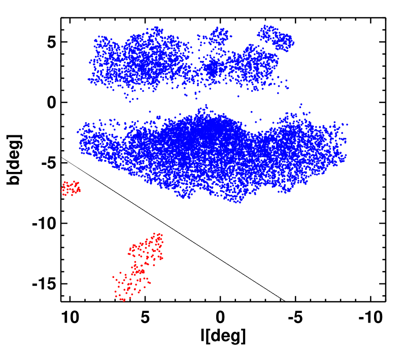
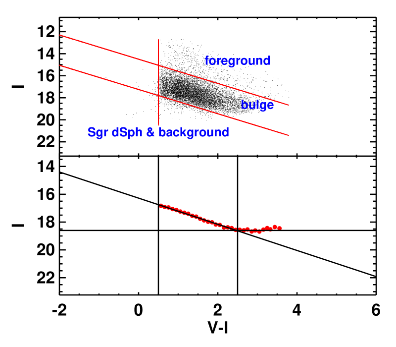
Figure 1: Left panel: Blue dots indicate the sample cleaned from the Sgr dSph galaxy and Galactic globular cluster M22 shown by red dots. Upper right panel: The selected sample for our analysis cleaned from foreground, background and other contaminant stars. Lower right panel: Binning cleaned data with bin size $0.1$ mag in the $V-I$ color show that the bulge sequence is linear down to $I\sim 18.6$ mag or $0.5\leq V-I\leq 2.5$ mag which is taken as the completeness limit for the present sample of bulge $\delta$ Scuti stars.

The remaining paper is organized as follows: In Section 2, we discuss the selection and cleaning of the $\delta$ Scuti stars taken from the OGLE-IV database. Section 3 deals with the methodology and the results obtained in the present study. Finally, the summary and conclusion of the present study are discussed in Section 4.

2 Selection and Cleaning of Data

The photometric data of the $\delta$ Scuti stars are taken from the data recently released by the OGLE-IV survey obtained using the $1.3$ meter Warsaw telescope situated at Las Campanas Observatory in Chille (Pietrukowicz et al., 2020). The OGLE-IV project has archived data of thousands of bulge $\delta$ Scuti stars from $2010$ to $2019$. The original OGLE sample consists of photometric data as well as the light curves of $10092$ $\delta$ Scuti stars in $V$ and $I$-bands. Seven fields around $(l,b)=(+5^{\circ},-13^{\circ})$ and a single field at $(l,b)=(+10^{\circ},-7^{\circ})$ cover the central part of the Sgr dSph galaxy and Galactic globular cluster M22, respectively (Pietrukowicz et al., 2020). The stars belonging to these regions are removed by drawing line: $b=0.8l-13.0$ as shown in left panel of Fig. 1. Then a clean sample of data free from the possible contamination of background and foreground sources is selected by closely following the selection criterion as prescribed by Pietrukowicz et al. (2015). The foreground (Halo and Disk stars; cf. Pietrukowicz et al. (2020)) and the background stars are removed by drawing lines at $I<14.5+1.1(V-I)$, $I>17.25+1.1(V-I)$ and $V-I<0.5$ as shown in the upper right panel of Fig. 1. This step reduces the number of $\delta$ Scuti stars for further analysis to $8,356$. For finding the photometric completeness of the sample of $\delta$ Scuti stars, we resort to the procedure as given by Pietrukowicz et al. (2015). The cleaned data are binned with a bin size $0.1$ as shown in the lower right panel of Fig. 1. It can be seen from the figure that the mean brightness of the bulge section is linear for $I\leq 18.6$ or $0.5\leq V-I\leq 2.5$. Hence following Pietrukowicz et al. (2015), we assume that our sample of $\delta$ Scuti stars is complete down to $I=18.6$ mag. Hence stars having $I\geq 18.6$ mag are removed from the clean sample which reduces the final number of $\delta$ Scuti stars to $7,440$ for further analysis.

3 Methodology

3.1 Distance to individual star

$\delta$ Scuti stars obey the following PL relation (Ziaali et al., 2019):

$$M_{V}= (-2.94\pm 0.06)\log{P}-(1.34\pm 0.06),~{}~{}~{}~{}\sigma_{\rm in}=0.34,$$ (1)

where $M_{V}$ is the absolute magnitude in $V$-band; $P$, the period of the star in days and $\sigma_{\rm in}=0.34$ mag denotes the intrinsic dispersion of the PL relation. The intrinsic dispersion is not mentioned in Ziaali et al. (2019) and has been obtained through a private communication. This empirical relation is based on more than $1100$ $\delta$ Scuti stars with good Gaia DR2 parallaxes in the Kepler field.

The absolute magnitudes are also calculated using the PL relation of McNamara (2011):

$$M_{V}= (-2.89\pm 0.13)\log{P}-(1.31\pm 0.10),~{}~{}~{}~{}\sigma_{\rm in}=0.07,$$ (2)

The true distance modulus is obtained using

$$\mu_{0}=\mu_{V}-R_{V}E(B-V),$$ (3)

where $\mu_{0}$ is the true distance modulus corrected for extinction; $\mu_{V}=\overline{m}_{V}-M_{V}$, the apparent distance modulus in the $V$-band. The values of $P$ and $\overline{m}_{V}$ are taken from the OGLE-IV database; $R_{V}$, the ratio of total to selective absorption in the V-band and $E(B-V)$ is the interstellar reddening along the line of sight. $R_{V}$ is taken to be $2.5$ (Nataf et al., 2013). $E(B-V)$ is estimated as follows: We know that

$$A_{V}=R_{V}E(B-V)$$ (4)

and from Cardelli et al. (1989) extinction law (Gonzalez et al., 2012a):

$$A_{J}=1.692E(J-K_{s}).$$ (5)

Dividing equation (5) by equation (4),

$$\frac{A_{J}}{A_{V}}= \frac{1.692E(J-K_{s})}{R_{V}E(B-V)}$$ (6)

$$\Rightarrow E(B-V)= \frac{1.692E(J-K_{s})}{R_{V}\left(\frac{A_{J}}{A_{V}}\right)}.$$ (7)

Here $\frac{A_{J}}{A_{V}}=0.26$, as obtained using Cardelli et al. (1989) extinction law and $E(J-K_{S})$ is obtained from the Gonzalez et al. (2012b) reddening map. Finally the distance is calculated using the following relation:

$$d= 10^{0.2\mu_{0}+1}.$$ (8)

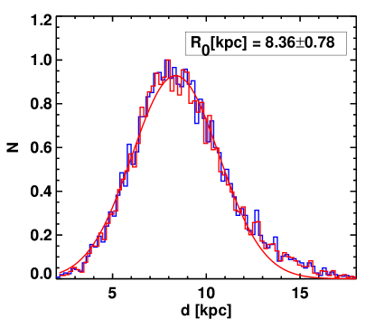
Figure 2: Histogram plot of the distance distribution of $\delta$ Scuti stars without and with cone-effect corrections as represented by blue and red colours, respectively. Solid line over plotted in red color denotes the Gaussian fit to the distance distribution corrected from the cone-effect.

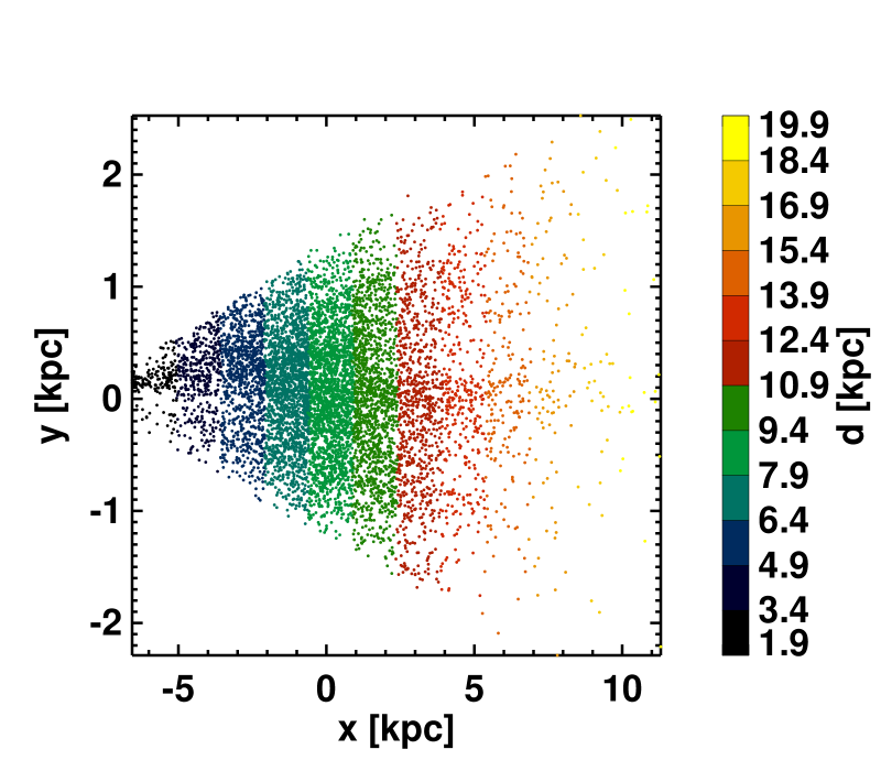
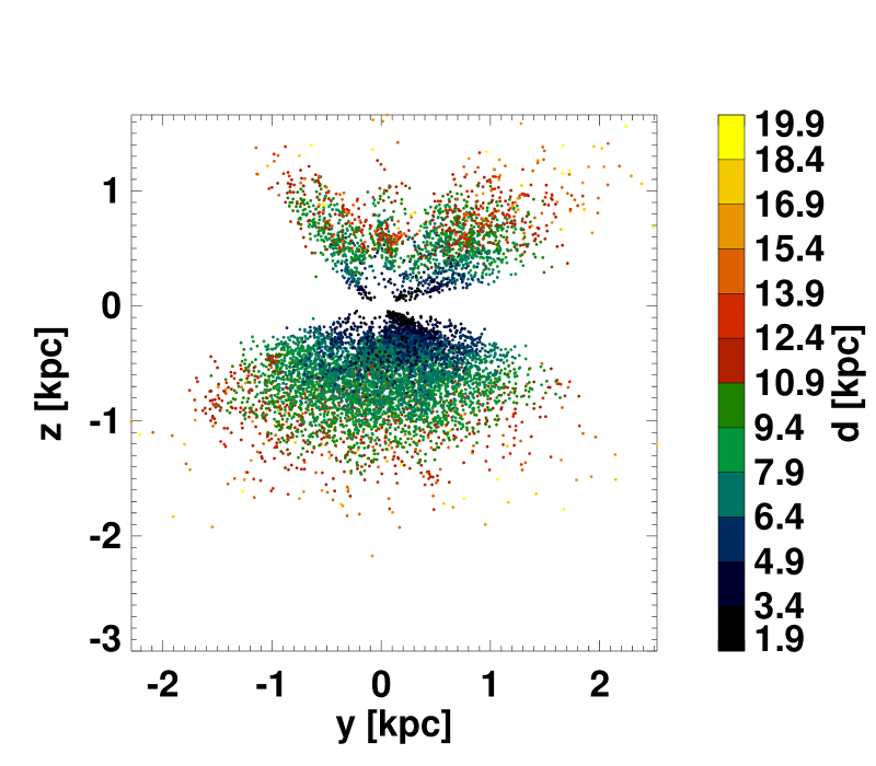
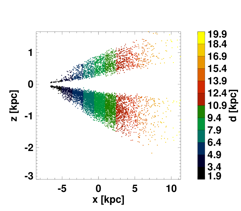
Figure 3: The projected distribution of bulge $\delta$ Scuti stars in Cartesian coordinate with the colour bar of distances.

A histogram plot of the distance is shown in Fig. 2. The distribution can be well represented by a Gaussian fit. The distribution is first corrected from the cone-effect and then fitted with a Gaussian profile. The peak of the distribution is found to be at $8.36\pm 0.78$ kpc which is taken as a preliminary estimate of $R_{0}$ for obtaining the radial number density profile of stars from the GC. Since the distance to individual stars is known, the following coordinate transformations are then used to convert Galactic coordinates into the Galacto-centric Cartesian coordinates:

$$x= d\cos{b}\cos{l}-R_{0}$$

$$y= d\cos{b}\sin{l}$$

$$z= d\sin{b},$$

where $x$-axis is directed along the Galactic anticenter; $y$-axis directed along the direction of Galactic rotation and $z$-axis is directed towards Galactic north. Colour-bar plots of the distribution of stars in the $xy,yz$ and $xz$-planes are shown in Fig. 3. The Galacto-centric distance is then calculated using

$$R= \sqrt{x^{2}+y^{2}+(z+z_{0})^{2}}.$$ (9)

Here $z_{0}$ is the Sun’s distance from the Galactic plane and is taken as $z_{0}=(20\pm 2)$ pc (Griv et al., 2021). Number density distribution of $R$ of the selected sample of $\delta$ Scuti stars and the corresponding cumulative distribution function (CDF) are shown in the left and right panels of Fig. 4, respectively.

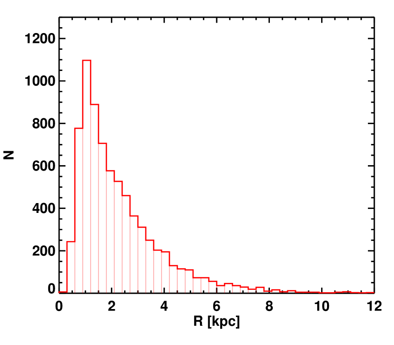
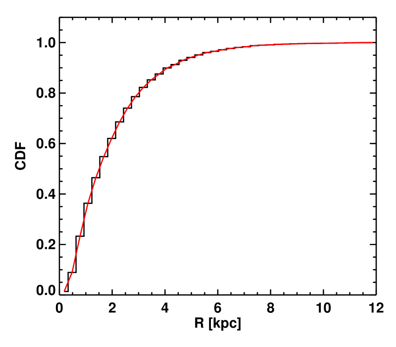
Figure 4: Left panel: The distribution of Galacto-centric distances of $\delta$ Scuti stars. Right panel: Cumulative distribution of Galacto-centric distances of $\delta$ Scuti stars.

3.2 Maximum Likelihood Parameter Estimation

We approximate the bulge as an ellipsoid given by

$$\frac{x^{2}}{a^{2}}+\frac{y^{2}}{b^{2}}+\frac{z^{2}}{c^{2}}= 1,$$ (10)

where $a,b,c$ are the normalized axes ($a\equiv 1$) of the ellipsoid with $a$, the major axis lying in the Galactic plane and pointing towards us and the two minor axes $b$ and $c$ lying in the Galactic plane and perpendicular to the Galactic plane, respectively. We assume the general case ($a\neq b\neq c$). The coordinate system $(x,y,z)$ is rotated in clockwise direction through $xy$-plane by an angle $\theta$ as

$$\begin{pmatrix}X\\ Y\\ Z\end{pmatrix}= \begin{pmatrix}\cos{\theta}&-\sin{\theta}&0\\ \sin{\theta}&\cos{\theta}&0\\ 0&0&1\end{pmatrix}\begin{pmatrix}x\\ y\\ z\end{pmatrix}.$$ (11)

Table 1: Geometrical parameters of the bulge for three different density distribution laws using the PL relation of Ziaali et al. (2019) with the given $\sigma_{\rm in}=0.34$ mag.

Model	$R_{\rm min}-R_{\rm max}$ [kpc]	$R_{0}$ [kpc]	$\theta~{}[^{\circ}]$	$a:b:c$
${\rm E_{1}}$	$0.05-1.5$	$8.310\pm 0.037$	$13.681\pm 5.621$	$1.000\pm 0.016:0.702\pm 0.011:0.877\pm 0.014$
	$0.05-2.0$	$8.024\pm 0.037$	$17.523\pm 5.327$	$1.000\pm 0.014:0.524\pm 0.007:0.640\pm 0.009$
	$0.05-2.5$	$8.033\pm 0.029$	$21.156\pm 4.864$	$1.000\pm 0.013:0.425\pm 0.005:0.515\pm 0.006$
	$0.05-3.0$	$8.013\pm 0.027$	$22.330\pm 4.267$	$1.000\pm 0.012:0.360\pm 0.004:0.435\pm 0.005$
	$0.05-3.5$	$8.044\pm 0.025$	$23.603\pm 4.507$	$1.000\pm 0.011:0.323\pm 0.004:0.390\pm 0.004$
	$0.05-4.0$	$8.050\pm 0.025$	$23.954\pm 4.471$	$1.000\pm 0.011:0.296\pm 0.003:0.359\pm 0.004$
${\rm E_{2}}$	$0.05-1.5$	$8.047\pm 0.032$	$17.794\pm 5.731$	$1.000\pm 0.016:0.674\pm 0.011:0.741\pm 0.011$
	$0.05-2.0$	$8.013\pm 0.027$	$20.718\pm 4.348$	$1.000\pm 0.014:0.508\pm 0.007:0.546\pm 0.007$
	$0.05-2.5$	$8.001\pm 0.025$	$23.019\pm 3.796$	$1.000\pm 0.012:0.412\pm 0.005:0.440\pm 0.005$
	$0.05-3.0$	$7.958\pm 0.023$	$22.443\pm 3.173$	$1.000\pm 0.011:0.350\pm 0.004:0.372\pm 0.004$
	$0.05-3.5$	$7.973\pm 0.022$	$22.872\pm 3.117$	$1.000\pm 0.011:0.314\pm 0.003:0.335\pm 0.003$
	$0.05-4.0$	$7.973\pm 0.021$	$22.745\pm 3.045$	$1.000\pm 0.011:0.289\pm 0.003:0.309\pm 0.003$
$\rm G$	$0.05-1.5$	$8.212\pm 0.019$	$14.542\pm 6.546$	$1.000\pm 0.013:0.705\pm 0.009:0.712\pm 0.008$
	$0.05-2.0$	$8.208\pm 0.017$	$20.285\pm 6.183$	$1.000\pm 0.011:0.531\pm 0.006:0.526\pm 0.005$
	$0.05-2.5$	$8.221\pm 0.015$	$27.389\pm 6.089$	$1.000\pm 0.010:0.431\pm 0.004:0.424\pm 0.004$
	$0.05-3.0$	$8.208\pm 0.014$	$27.650\pm 5.242$	$1.000\pm 0.009:0.365\pm 0.003:0.359\pm 0.003$
	$0.05-3.5$	$8.231\pm 0.013$	$30.764\pm 5.944$	$1.000\pm 0.009:0.327\pm 0.003:0.323\pm 0.003$
	$0.05-4.0$	$8.239\pm 0.010$	$31.491\pm 0.562$	$1.000\pm 0.006:0.300\pm 0.006:0.297\pm 0.006$

Table 2: Geometrical parameters of the bulge for three different density distribution laws using the PL relation of Ziaali et al. (2019) assuming $\sigma_{\rm in}=0.2$ mag.

Model	$R_{\rm min}-R_{\rm max}$ [kpc]	$R_{0}$ [kpc]	$\theta~{}[^{\circ}]$	$a:b:c$
${\rm E_{1}}$	$0.05-1.5$	$8.082\pm 0.036$	$11.183\pm 5.373$	$1.000\pm 0.016:0.717\pm 0.011:0.897\pm 0.014$
	$0.05-2.0$	$8.118\pm 0.031$	$17.808\pm 5.163$	$1.000\pm 0.013:0.537\pm 0.007:0.657\pm 0.009$
	$0.05-2.5$	$8.187\pm 0.028$	$27.285\pm 5.887$	$1.000\pm 0.012:0.442\pm 0.005:0.539\pm 0.006$
	$0.05-3.0$	$8.175\pm 0.026$	$29.173\pm 5.276$	$1.000\pm 0.011:0.382\pm 0.004:0.465\pm 0.005$
	$0.05-3.5$	$8.178\pm 0.025$	$29.756\pm 5.113$	$1.000\pm 0.011:0.344\pm 0.004:0.419\pm 0.005$
	$0.05-4.0$	$8.181\pm 0.024$	$30.395\pm 5.077$	$1.000\pm 0.011:0.322\pm 0.003:0.391\pm 0.004$
$\rm E_{2}$	$0.05-1.5$	$8.079\pm 0.031$	$13.552\pm 4.599$	$1.000\pm 0.015:0.686\pm 0.010:0.757\pm 0.011$
	$0.05-2.0$	$8.097\pm 0.026$	$19.283\pm 4.174$	$1.000\pm 0.013:0.519\pm 0.007:0.559\pm 0.007$
	$0.05-2.5$	$8.138\pm 0.024$	$26.021\pm 4.303$	$1.000\pm 0.012:0.429\pm 0.005:0.460\pm 0.005$
	$0.05-3.0$	$8.118\pm 0.023$	$26.865\pm 3.807$	$1.000\pm 0.011:0.370\pm 0.004:0.396\pm 0.004$
	$0.05-3.5$	$8.114\pm 0.022$	$26.993\pm 3.549$	$1.000\pm 0.011:0.334\pm 0.004:0.358\pm 0.004$
	$0.05-4.0$	$8.110\pm 0.021$	$26.893\pm 3.459$	$1.000\pm 0.011:0.311\pm 0.003:0.335\pm 0.003$
${\rm G}$	$0.05-1.5$	$8.277\pm 0.018$	$9.273\pm 5.503$	$1.000\pm 0.012:0.719\pm 0.008:0.734\pm 0.008$
	$0.05-2.0$	$8.305\pm 0.016$	$17.344\pm 6.136$	$1.000\pm 0.010:0.542\pm 0.005:0.539\pm 0.005$
	$0.05-2.5$	$8.342\pm 0.014$	$32.884\pm 7.593$	$1.000\pm 0.009:0.446\pm 0.004:0.443\pm 0.004$
	$0.05-3.0$	$8.333\pm 0.013$	$35.086\pm 6.690$	$1.000\pm 0.009:0.383\pm 0.003:0.380\pm 0.003$
	$0.05-3.5$	$8.338\pm 0.013$	$36.448\pm 6.715$	$1.000\pm 0.008:0.344\pm 0.003:0.342\pm 0.003$
	$0.05-4.0$	$8.340\pm 0.013$	$37.162\pm 6.781$	$1.000\pm 0.008:0.319\pm 0.003:0.318\pm 0.002$

Table 3: Geometrical parameters of the bulge for three different density distribution laws using the PL relation of Ziaali et al. (2019) assuming $\sigma_{\rm in}=0.1$ mag.

Model	$R_{\rm min}-R_{\rm max}$ [kpc]	$R_{0}$ [kpc]	$\theta~{}[^{\circ}]$	$a:b:c$
${\rm E_{1}}$	$0.05-1.5$	$8.167\pm 0.035$	$12.852\pm 6.271$	$1.000\pm 0.015:0.712\pm 0.011:0.900\pm 0.013$
	$0.05-2.0$	$8.193\pm 0.030$	$22.322\pm 6.085$	$1.000\pm 0.013:0.548\pm 0.007:0.672\pm 0.008$
	$0.05-2.5$	$8.194\pm 0.027$	$25.495\pm 5.546$	$1.000\pm 0.012:0.450\pm 0.005:0.553\pm 0.007$
	$0.05-3.0$	$8.218\pm 0.026$	$27.024\pm 5.735$	$1.000\pm 0.011:0.398\pm 0.004:0.485\pm 0.005$
	$0.05-3.5$	$8.224\pm 0.025$	$29.395\pm 5.673$	$1.000\pm 0.011:0.360\pm 0.004:0.438\pm 0.005$
	$0.05-4.0$	$8.216\pm 0.024$	$30.508\pm 5.323$	$1.000\pm 0.011:0.333\pm 0.004:0.405\pm 0.004$
$\rm E_{2}$	$0.05-1.5$	$8.146\pm 0.030$	$16.277\pm 5.084$	$1.000\pm 0.015:0.686\pm 0.010:0.765\pm 0.011$
	$0.05-2.0$	$8.150\pm 0.026$	$23.104\pm 4.429$	$1.000\pm 0.013:0.529\pm 0.007:0.572\pm 0.007$
	$0.05-2.5$	$8.138\pm 0.024$	$24.560\pm 3.947$	$1.000\pm 0.012:0.437\pm 0.005:0.473\pm 0.005$
	$0.05-3.0$	$8.147\pm 0.022$	$24.787\pm 3.847$	$1.000\pm 0.011:0.387\pm 0.004:0.417\pm 0.004$
	$0.05-3.5$	$8.146\pm 0.021$	$25.936\pm 3.694$	$1.000\pm 0.011:0.350\pm 0.004:0.376\pm 0.004$
	$0.05-4.0$	$8.136\pm 0.021$	$26.445\pm 3.471$	$1.000\pm 0.011:0.323\pm 0.003:0.348\pm 0.003$
${\rm G}$	$0.05-1.5$	$8.313\pm 0.018$	$9.870\pm 5.861$	$1.000\pm 0.012:0.718\pm 0.008:0.741\pm 0.008$
	$0.05-2.0$	$8.336\pm 0.015$	$21.474\pm 6.528$	$1.000\pm 0.010:0.552\pm 0.005:0.551\pm 0.005$
	$0.05-2.5$	$8.341\pm 0.014$	$26.522\pm 6.283$	$1.000\pm 0.009:0.453\pm 0.004:0.454\pm 0.004$
	$0.05-3.0$	$8.358\pm 0.013$	$28.474\pm 6.903$	$1.000\pm 0.009:0.398\pm 0.003:0.396\pm 0.003$
	$0.05-3.5$	$8.364\pm 0.013$	$33.453\pm 6.929$	$1.000\pm 0.008:0.358\pm 0.003:0.354\pm 0.003$
	$0.05-4.0$	$8.360\pm 0.013$	$35.108\pm 6.719$	$1.000\pm 0.008:0.327\pm 0.003:0.326\pm 0.002$

Table 4: Geometrical parameters of the bulge for three different density distribution laws using the PL relation of McNamara (2011) with the given $\sigma_{\rm in}=0.07$ mag.

Model	$R_{\rm min}-R_{\rm max}$ [kpc]	$R_{0}$ [kpc]	$\theta~{}[^{\circ}]$	$a:b:c$
${\rm E_{1}}$	$0.05-1.5$	$8.327\pm 0.035$	$14.568\pm 7.788$	$1.000\pm 0.015:0.731\pm 0.011:0.925\pm 0.014$
	$0.05-2.0$	$8.313\pm 0.030$	$24.334\pm 6.479$	$1.000\pm 0.013:0.551\pm 0.007:0.681\pm 0.009$
	$0.05-2.5$	$8.313\pm 0.027$	$27.997\pm 6.011$	$1.000\pm 0.012:0.464\pm 0.005:0.567\pm 0.007$
	$0.05-3.0$	$8.348\pm 0.025$	$31.876\pm 6.431$	$1.000\pm 0.011:0.405\pm 0.005:0.494\pm 0.006$
	$0.05-3.5$	$8.342\pm 0.024$	$31.012\pm 6.059$	$1.000\pm 0.011:0.365\pm 0.004:0.445\pm 0.005$
	$0.05-4.0$	$8.341\pm 0.024$	$31.506\pm 5.918$	$1.000\pm 0.011:0.339\pm 0.004:0.413\pm 0.004$
${\rm E_{2}}$	$0.05-1.5$	$8.319\pm 0.030$	$18.104\pm 6.523$	$1.000\pm 0.015:0.701\pm 0.010:0.783\pm 0.011$
	$0.05-2.0$	$8.271\pm 0.026$	$24.730\pm 4.776$	$1.000\pm 0.013:0.530\pm 0.007:0.578\pm 0.007$
	$0.05-2.5$	$8.261\pm 0.024$	$26.672\pm 4.266$	$1.000\pm 0.012:0.449\pm 0.005:0.484\pm 0.005$
	$0.05-3.0$	$8.278\pm 0.022$	$28.257\pm 4.263$	$1.000\pm 0.011:0.392\pm 0.004:0.423\pm 0.004$
	$0.05-3.5$	$8.261\pm 0.021$	$26.758\pm 3.880$	$1.000\pm 0.011:0.353\pm 0.004:0.381\pm 0.004$
	$0.05-4.0$	$8.257\pm 0.021$	$26.643\pm 3.687$	$1.000\pm 0.011:0.328\pm 0.003:0.354\pm 0.004$
$\rm G$	$0.05-1.5$	$8.452\pm 0.018$	$10.747\pm 7.314$	$1.000\pm 0.012:0.733\pm 0.008:0.756\pm 0.008$
	$0.05-2.0$	$8.440\pm 0.015$	$23.152\pm 6.629$	$1.000\pm 0.010:0.554\pm 0.005:0.557\pm 0.005$
	$0.05-2.5$	$8.446\pm 0.014$	$29.501\pm 6.628$	$1.000\pm 0.009:0.466\pm 0.004:0.463\pm 0.004$
	$0.05-3.0$	$8.470\pm 0.013$	$35.505\pm 7.775$	$1.000\pm 0.009:0.404\pm 0.003:0.402\pm 0.003$
	$0.05-3.5$	$8.467\pm 0.013$	$33.201\pm 7.226$	$1.000\pm 0.008:0.361\pm 0.003:0.360\pm 0.003$
	$0.05-4.0$	$8.470\pm 0.013$	$33.868\pm 7.296$	$1.000\pm 0.008:0.333\pm 0.003:0.332\pm 0.003$

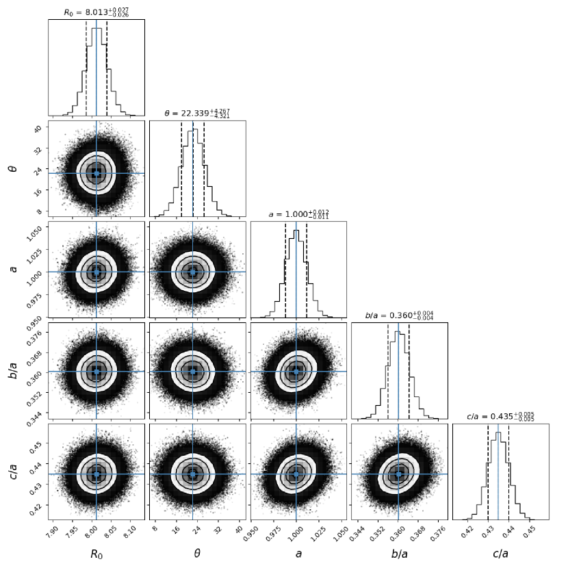
Figure 5: Marginalized posterior distribution and uncertainties of the model parameters obtained from the MCMC analysis for the $\rm E_{1}$-model with $R_{\rm max}=3$ kpc considering Ziaali et al. (2019) PL relation with $\sigma_{\rm in}=0.34$ mag. The statistical uncertainties listed here are measured with the sample mean and $16$th (down) and $84$th(up) percentile differences. The black dashed vertical lines on each histogram represent the $16$th, $50$th and $84$th percentiles, respectively. This plot uses the corner package (Foreman-Mackey, 2016).

Table 5: BIC and AIC values for the optimized parameters of different models.

PL relation	$\sigma_{\rm in}$	Model	$R_{\rm min}-R_{\rm max}$ [kpc]	BIC	AIC
Ziaali et al. (2019)	$0.34$	$\rm E_{1}$	$0.05-3.0$	$27335.241$	$27345.241$
		$\rm E_{2}$	$0.05-3.0$	$34735.598$	$34702.382$
		$\rm G$	$0.05-3.0$	$40794.816$	$40761.599$
Ziaali et al. (2019)	$0.2~{}(\text{assumed})$	$\rm E_{1}$	$0.05-3.0$	$27494.606$	$27504.606$
		$\rm E_{2}$	$0.05-3.0$	$36617.056$	$36583.592$
		$\rm G$	$0.05-3.0$	$41609.247$	$41575.782$
Ziaali et al. (2019)	$0.1~{}(\text{assumed})$	$\rm E_{1}$	$0.05-3.0$	$26937.706$	$26947.706$
		$\rm E_{2}$	$0.05-3.0$	$36992.276$	$36958.719$
		$\rm G$	$0.05-3.0$	$41126.608$	$41093.050$
McNamara (2011)	$0.07$	$\rm E_{1}$	$0.05-3.0$	$27847.405$	$27857.405$
		$\rm E_{2}$	$0.05-3.0$	$37441.682$	$37408.122$
		$\rm G$	$0.05-3.0$	$41370.151$	$41336.591$

For the spatial distribution of stars with $R\geq 1.0$ kpc, the bulge can be approximated with various kinds of density models (Dwek et al., 1995) and the following three models are selected for the ML analysis: two Exponential types ($\rm E_{1}$ and $\rm E_{2}$) and one Gaussian ($\rm G$) type which are given as follows (Dwek et al., 1995; Rattenbury et al., 2007; Cao et al., 2013):

$$\text{Model}~{}{\rm E_{1}}:\rho= \rho_{0}\exp\left(-R\right)$$ (12)

$$\text{Model}~{}{\rm E_{2}}:\rho= \rho_{0}k_{0}\left(R_{\rm s}\right)$$ (13)

$$\text{Model}~{}~{}{\rm G}:\rho= \rho_{0}\exp\left({-0.5R_{s}^{2}}\right).$$ (14)

Here $\rho_{0}$ is the unknown normalization constant and is a function of $R,\theta,a,b,c$; $\theta$ is the angle at which the major axis lying in the Galactic plane is tilted with respect to the line joining the GC and the Sun; $a,b,c$ are the normalized axes of the ellipsoidal distribution of the bulge. Here $k_{0}$ denotes the modified Bessel function of second kind. Models $\rm E_{1},\rm E_{2}$ and $\rm G$ represent exponential, exponential boxy and Gaussian-triaxial bulges, respectively (Dwek et al., 1995). The expressions of $R$ and $R_{s}$ are respectively given by (Dwek et al., 1995):

$$R= \left[\left(\frac{x}{a}\right)^{2}+\left(\frac{y}{b}\right)^{2}+\left(\frac{z}{c}\right)^{2}\right]^{\frac{1}{2}}.$$ (15)

$$R_{\rm s}= \left\{\left[\left(\frac{x}{a}\right)^{2}+\left(\frac{y}{b}\right)^{2}\right]^{2}+\left(\frac{z}{c}\right)^{4}\right\}^{\frac{1}{4}}.$$ (16)

The value of $\rho_{0}$ can be obtained using the normalization condition:

$$\int_{V}\rho dV= 1,$$ (17)

which can be expressed as

$$4\pi abc\rho_{0}\int_{R_{\rm min}}^{R_{\rm max}}R^{2}\rho dR= 1.$$ (18)

The likelihood function for a given density model is defined as

$$L= \prod_{i=1}^{n}\rho_{i}(R;R_{0},\theta,a,b,c)$$

$$\Rightarrow\ln{L}= \sum\limits_{i=1}^{n}\ln{\rho_{i}(R;R_{0},\theta,a,b,c)},$$ (19)

where $n$ denotes the total number of stars. $R_{\rm max}$ and $R_{\rm min}$ denote the lower and the upper limits of the integration, respectively. We take $R_{\rm min}=0.05$ kpc and $R_{\rm max}=1.5,2.0,2.5,3.0,3.5,4.0$ kpc. From the Fig. 4, it can be easily seen that most of the stars lie within $R=4.0$ kpc and the number of stars falls rapidly above $R=5.0$ kpc. As logarithm is monotonically increasing function, we use log-likelihood rather than likelihood function for the mathematical convenience. We find the values of the parameters which maximizes $\ln{L}$ in five dimensional parameter space using python implemented limited-memory BFGS optimization method ‘L-BFGS’ (Byrd et al., 1995). More refined values of these parameters and their statistical uncertainties are explored using MCMC analysis in a Bayesian framework (Foreman-Mackey et al., 2013). The posterior distribution is sampled with $1000$ walkers, $1000$ iterations and $100$ burn-in using the affine-invariant MCMC ensemble sampler emcee-Python package (Foreman-Mackey et al., 2013).

To find the ML parameters, we have provided initial guesses as well as the minimum and the maximum limits for each of the parameters. We have run ‘L-BFGS’ several times based on different initial guesses within the range for convergence. The ML results obtained from the ‘L-BFGS’ method are then used to initialize the walkers in a tiny Gaussian ball around these values for the MCMC analysis (Foreman-Mackey et al., 2013). The MCMC chains are used to compute the marginalized posterior distributions for each of the parameters. As the distributions are highly symmetrical as shown in Fig. 5, the mean and the median of the distributions will be the same. The mean of each of the distribution ($50$th percentile) is taken as the robust measure of the best fit value with the statistical uncertainties measured up and down to the $16$th and $84$th percentiles, respectively. The results obtained from the MCMC analysis for different PL relations varying the intrinsic dispersion values are listed in Tables 1, 2,  3, 4. Tables 1,2,3 list the values of geometrical parameters employing Ziaali et al. (2019) PL relation considering $\sigma_{\rm in}=0.34,~{}0.2,~{}0.1$ mag, respectively. On the other hand, Table 4 lists the parameter values employing McNamara (2011) PL relation with $\sigma_{\rm in}=0.07$ mag. A sampling acceptance rate of $\sim 0.5$ is achieved in each of the MCMC analyses.

3.3 Best Fitting Model

Bayesian Information Criterion(BIC) is a model selection criterion among a class of parametric models (Schwarz, 1978). Akaike Information Criterion (AIC) is also a model selection criteria which measures the goodness of fit of a statistical model (Akaike, 1974). The best model minimizes both the AIC and BIC values for the given set of parameter values. They are defined as:

$${\rm BIC}= p\ln{n}-2\ln{\hat{L}},$$ (20)

$${\rm AIC}= 2p-2\ln{\hat{L}}.$$ (21)

Here $p$ denotes the number of parameters of the model; $n$, the total number of stars; $\hat{L}$, the maximum likelihood values given the parameters of the models. Among the three models considered in the present study, both the BIC and AIC values are the lowest for the ‘$\rm E_{1}$-model’. This implies that $\rm E_{1}$-model is the best fitted model to the number density of $\delta$ Scuti stars for the Ziaali et al. (2019) PL relation assuming $\sigma_{\rm in}=0.1$ mag (Table 5). However, this is not the actual value of $\sigma_{\rm in}$. The Ziaali et al. (2019) relation was obtained with $\sigma_{\rm in}=0.34$ mag. The AIC and BIC values obtained using $\sigma_{\rm in}=0.34$ mag also suggest that the model $\rm E_{1}$ is the best-fitted model among all the three models considered (Table 5). Furthermore, comparing both the AIC and the BIC values obtained for the $\rm E_{1}$ model between Ziaali et al. (2019) with $\sigma_{\rm in}=0.34$ mag and McNamara (2011), it can be clearly seen from Table 5 that the use of Ziaali et al. (2019) relation with $\sigma_{\rm in}=0.34$ mag gives their lowest values. Therefore, the final values of the parameters as quoted in the present study are those obtained using the Ziaali et al. (2019) relation with $\sigma_{\rm in}=0.34$ mag. Fig. 5 depicts a representative plot of the marginalized posterior distribution and uncertainties of the model parameters obtained from the MCMC analysis for the $\rm E_{1}$-model up to $R_{\rm max}=3$ kpc conidering Ziaali et al. (2019) relation with $\sigma_{\rm in}=0.34$ mag. The statistical uncertainties are measured with the sample mean and $16$th (down) and $84$th (up) percentile differences. The black dashed vertical lines on each histogram represent the $16$th, $50$th and $84$th percentiles, respectively.

3.4 Systematic Uncertainty in $R_{0}$

Systematic uncertainty in $R_{0}$ in the present study relies on two factors: errors in the extinction values as well as the errors due to the uncertainty in the coefficients of the PL relation $(\sim 0.090)$. The error in $E(B-V)$ is calculated using $\sigma_{E(J-K_{s})}=0.02$ mag (Gonzalez et al., 2012b). Taking into account all these errors, the uncertainty in distance modulus is found to be $\sigma_{\mu,{\rm sys}}=0.159$ mag which corresponds to a systematic uncertainty in $R_{0}$ with a value $\sigma_{R_{0},{\rm sys}}=0.586$ kpc.

4 Summary and Conclusion

In the present study, we have carried out an analysis of the structure of the Galactic bulge using a clean sample of more than $7440$ high latitude $\delta$ Scuti stars ($\left|b\right|>1^{\circ}$) recently released by the OGLE-IV survey. The distribution of the number density of stars as a function of different range of Galacto-centric distances has been modelled using three functions: two exponential types ($\rm E_{1}$ and $\rm E_{2}$) and one Gaussian type ($G$). The geometrical parameters of the bulge are calculated starting from $R_{\rm min}=0.05$ kpc up to various maximum values of $R_{\rm max}$ till $4$ kpc based on ML estimation. Refined values of these parameters along with their statistical uncertainties are explored using a fully Bayesian MCMC analysis. The values of the model parameters are found to vary slightly with different values of $R_{\rm max}$. Among all the three models chosen for the present study, it is found from the statistical analysis that the distribution of the number density of the bulge $\delta$ Scuti stars can be best fitted with the exponential triaxial model ‘$\rm E_{1}$’ using the Ziaali et al. (2019) PL relation with $\sigma_{\rm in}=0.34$ mag. It is to be noted that the other values of $\sigma_{\rm in}=0.1,~{}0.2$ mag were considered in the relation to see the effect of reduced values of $\sigma_{\rm in}$ and are not the real values. Therefore, the parameters corresponding to the $\rm E_{1}$ model obtained with $\sigma_{\rm in}=0.34$ mag are chosen as the best parameters describing the structure of the bulge. The final values of the parameters are calculated from their weighted averages obtained with $R_{\rm max}=2.0,2.5,3.0,3.5,4.0$ kpc using the model $\rm E_{1}$ corresponding to the Ziaali et al. (2019) PL relation with $\sigma_{\rm in}=0.34$ mag. The errors of the parameters quoted for different values of $R_{\rm max}$ denote the statistical errors obtained from the MCMC analysis. The modelling of the bulge distribution with the best-fitted density model $\rm E_{1}$ yields the following results:

1. The mean distance to the GC is obtained as $R_{0}=8.034\pm 0.012_{\rm stat}\pm 0.586_{\rm sys}$ kpc which is consistent with most of the recent studies (Pietrukowicz et al., 2015; Bhardwaj et al., 2017; Gravity Collaboration et al., 2019; Griv et al., 2019; Griv et al., 2020, 2021). Pietrukowicz et al. (2015) estimated this value to be $8.27$ kpc using the distance distribution of the bulge RR Lyrae stars based on the OGLE-III data. Using a median statistical analysis of $28$ independent values of recent $R_{0}$, Camarillo et al. (2018) obtained $R_{0}=8.0\pm 0.3$ kpc. On the other hand, Griv et al. (2020, 2021) estimated the values of $R_{0}$ as $8.28\pm 0.14$ kpc and $8.35\pm 0.10$ kpc by employing a maximum likelihood analysis on the photometric data of OGLE RRab stars taken from Soszyński et al. (2014) and $715$ Type II Cepheids in the Galactic bulge from VVV (VISTA Variables in the Via Lactea), respectively. Besides these values, Gravity Collaboration et al. (2019) found $R_{0}=8.178\pm 0.013_{\rm stat}\pm 0.022_{\rm sys}$ kpc following the star S2 in its orbit around the massive black hole Sgr A^⋆; this is a direct method without relying on any calibrators. By correcting the aberration effect from the same data as in Gravity Collaboration et al. (2019), Gravity Collaboration et al. (2021) estimated $R_{0}=8.275\pm 0.009_{\rm stat.}\pm 0.033_{\rm sys.}$ kpc. However, Do et al. (2019) found $R_{0}=7.94\pm 0.05_{\rm stat.}\pm 0.03_{\rm sys.}$ kpc by independently analyzing the orbit of S2 star. On the other hand, using $21$ individual estimates of $R_{0}$ from $2017$ onwards, Bobylev & Bajkova (2021) calculated the best value to be $R_{0}=8.1\pm 0.1$ kpc.

2. The inclination angle made by the major axis lying in the Galactic plane with the Sun-GC line is found to be $\theta=22^{\circ}.006\pm 2^{\circ}.078$. This value is quite in good agreement with other values as obtained in the literature (Dékány et al. (2013); Pietrukowicz et al. (2015); Simion et al. (2017); Grady et al. (2020); Du et al. (2020) and references therein).

3. The axes ratios are found to be $a:b:c=1.000\pm 0.005:0.348\pm 0.002:0.421\pm 0.002$. Smaller values of $b$ and $c$ as compared to the values of $a$ obtained for $R\geq 2.0$ kpc indicate that the distribution of the $\delta$ Scuti stars in the bulge follows a bar-like structure with a bar angle of $22^{\circ}.006\pm 2^{\circ}.078$.

DATA AVAILABILITY

The data underlying this article are available at ftp://ftp.astrouw.edu.pl/ogle/ogle4/OCVS/blg/dsct/. The derived data generated in this research will be shared on reasonable request to the corresponding author.

References

• Akaike (1974) Akaike H., 1974, IEEE Transactions on Automatic Control, 19, 716
• Antoci et al. (2019) Antoci V., et al., 2019, MNRAS, 490, 4040
• Babusiaux & Gilmore (2005) Babusiaux C., Gilmore G., 2005, MNRAS, 358, 1309
• Bedding et al. (2020) Bedding T. R., et al., 2020, Nature, 581, 147
• Bhardwaj et al. (2017) Bhardwaj A., et al., 2017, A&A, 605, A100
• Binney et al. (1997) Binney J., Gerhard O., Spergel D., 1997, MNRAS, 288, 365
• Bland-Hawthorn & Gerhard (2016) Bland-Hawthorn J., Gerhard O., 2016, ARA&A, 54, 529
• Blitz & Spergel (1991) Blitz L., Spergel D. N., 1991, ApJ, 379, 631
• Bobylev & Bajkova (2021) Bobylev V. V., Bajkova A. T., 2021, Astronomy Reports, 65, 498
• Bolker (2008) Bolker B. M., 2008, Likelihood and All That. Princeton University Press, pp 169–221, http://www.jstor.org/stable/j.ctvcm4g37.9
• Byrd et al. (1995) Byrd R., Lu P., Nocedal J., Zhu C., 1995, SIAM Journal of Scientific Computing, 16, 1190
• Camarillo et al. (2018) Camarillo T., Mathur V., Mitchell T., Ratra B., 2018, PASP, 130, 024101
• Cao et al. (2013) Cao L., Mao S., Nataf D., Rattenbury N. J., Gould A., 2013, MNRAS, 434, 595
• Cardelli et al. (1989) Cardelli J. A., Clayton G. C., Mathis J. S., 1989, ApJ, 345, 245
• Carroll & Ostlie (2017) Carroll B., Ostlie D., 2017, An Introduction to Modern Astrophysics. Cambridge University Press, %****␣ds_like.bbl␣Line␣100␣****https://books.google.co.in/books?id=PY0wDwAAQBAJ
• Chang et al. (2013) Chang S. W., Protopapas P., Kim D. W., Byun Y. I., 2013, AJ, 145, 132
• Dékány et al. (2013) Dékány I., Minniti D., Catelan M., Zoccali M., Saito R. K., Hempel M., Gonzalez O. A., 2013, ApJL, 776, L19
• Dékány et al. (2019) Dékány I., Hajdu G., Grebel E. K., Catelan M., 2019, ApJ, 883, 58
• Do et al. (2019) Do T., et al., 2019, Science, 365, 664
• Du et al. (2020) Du H., Mao S., Athanassoula E., Shen J., Pietrukowicz P., 2020, MNRAS, 498, 5629
• Dwek et al. (1995) Dwek E., et al., 1995, ApJ, 445, 716
• Foreman-Mackey (2016) Foreman-Mackey D., 2016, The Journal of Open Source Software, 1, 24
• Foreman-Mackey et al. (2013) Foreman-Mackey D., Hogg D. W., Lang D., Goodman J., 2013, PASP, 125, 306
• Freedman & Kaufmann (2007) Freedman R., Kaufmann W., 2007, Universe. W. H. Freeman, https://books.google.co.in/books?id=jCd5vwEACAAJ
• Gonzalez & Gadotti (2016) Gonzalez O. A., Gadotti D., 2016, The Milky Way Bulge: Observed Properties and a Comparison to External Galaxies. p. 199, doi:10.1007/978-3-319-19378-6_9
• Gonzalez et al. (2012a) Gonzalez O. A., Rejkuba M., Zoccali M., Valenti E., Minniti D., Schultheis M., Tobar R., Chen B., 2012a, A&A, 543, A13
• Gonzalez et al. (2012b) Gonzalez O. A., Rejkuba M., Zoccali M., Valenti E., Minniti D., Schultheis M., Tobar R., Chen B., 2012b, A&A, 543, A13
• Goupil et al. (2005) Goupil M. J., Dupret M. A., Samadi R., Boehm T., Alecian E., Suarez J. C., Lebreton Y., Catala C., 2005, Journal of Astrophysics and Astronomy, 26, 249
• Grady et al. (2020) Grady J., Belokurov V., Evans N. W., 2020, MNRAS, 492, 3128
• Gravity Collaboration et al. (2019) Gravity Collaboration et al., 2019, AAP, 625, L10
• Gravity Collaboration et al. (2021) Gravity Collaboration et al., 2021, AAP, 647, A59
• Griv et al. (2019) Griv E., Gedalin M., Jiang I.-G., 2019, MNRAS, 484, 218
• Griv et al. (2020) Griv E., Gedalin M., Pietrukowicz P., Majaess D., Jiang I.-G., 2020, MNRAS, 499, 1091
• Griv et al. (2021) Griv E., Gedalin M., Pietrukowicz P., Majaess D., Jiang I.-G., 2021, MNRAS, 502, 4194
• Guzik (2021) Guzik J. A., 2021, Frontiers in Astronomy and Space Sciences, 8, 55
• Jayasinghe et al. (2020) Jayasinghe T., et al., 2020, MNRAS, 493, 4186
• Majaess (2010) Majaess D., 2010, ACTAA, 60, 55
• Majaess et al. (2009) Majaess D. J., Turner D. G., Lane D. J., 2009, MNRAS, 398, 263
• Majaess et al. (2018) Majaess D., Dékány I., Hajdu G., Minniti D., Turner D., Gieren W., 2018, Ap&SS, 363, 127
• McNamara (1997) McNamara D., 1997, Publications of the Astronomical Society of the Pacific, 109, 1221
• McNamara (2011) McNamara D. H., 2011, AJ, 142, 110
• McNamara & Augason (1962) McNamara D. H., Augason G., 1962, ApJ, 135, 64
• Minniti et al. (2010) Minniti D., et al., 2010, NA, 15, 433
• Nataf et al. (2013) Nataf D. M., et al., 2013, ApJ, 769, 88
• Nemec et al. (2017) Nemec J. M., Balona L. A., Murphy S. J., Kinemuchi K., Jeon Y.-B., 2017, MNRAS, 466, 1290
• Picaud & Robin (2004) Picaud S., Robin A. C., 2004, A&A, 428, 891
• Pietrukowicz et al. (2012) Pietrukowicz P., et al., 2012, ApJ, 750, 169
• Pietrukowicz et al. (2015) Pietrukowicz P., et al., 2015, ApJ, 811, 113
• Pietrukowicz et al. (2020) Pietrukowicz P., et al., 2020, ACTAA, 70, 241
• Poro et al. (2021) Poro A., et al., 2021, arXiv e-prints, p. arXiv:2102.10136
• Rastorguev et al. (1994) Rastorguev A. S., Pavlovskaya E. D., Durlevich O. V., Filippova A. A., 1994, AstL, 20, 591
• Rattenbury et al. (2007) Rattenbury N. J., Mao S., Sumi T., Smith M. C., 2007, MNRAS, 378, 1064
• Reid (1993) Reid M. J., 1993, ARA&A, 31, 345
• Reid et al. (2019) Reid M. J., et al., 2019, ApJ, 885, 131
• Rich (2013) Rich R. M., 2013, The Galactic Bulge. Springer Netherlands, Dordrecht, pp 271–346, doi:10.1007/978-94-007-5612-0_6, https://doi.org/10.1007/978-94-007-5612-0_6
• Saito et al. (2012) Saito R. K., et al., 2012, AAP, 544, A147
• Sanchez Arias et al. (2018) Sanchez Arias J. P., Romero A. D., Córsico A. H., Pelisoli I., Antoci V., Kepler S. O., Althaus L. G., Corti M. A., 2018, A&A, 616, A80
• Schwarz (1978) Schwarz G., 1978, The Annals of Statistics, 6, 461
• Simion et al. (2017) Simion I. T., Belokurov V., Irwin M., Koposov S. E., Gonzalez-Fernandez C., Robin A. C., Shen J., Li Z. Y., 2017, MNRAS, 471, 4323
• Simion et al. (2021) Simion I. T., Shen J., Koposov S. E., Ness M., Freeman K., Bland-Hawthorn J., Lewis G. F., 2021, MNRAS, 502, 1740
• Skrutskie et al. (2006) Skrutskie M. F., et al., 2006, AJ, 131, 1163
• Soszyński et al. (2014) Soszyński I., et al., 2014, ACTAA, 64, 177
• Stanek et al. (1994) Stanek K. Z., Mateo M., Udalski A., Szymanski M., Kaluzny J., Kubiak M., 1994, ApJ, 429, L73
• Stanek et al. (1997) Stanek K. Z., Udalski A., SzymaŃski M., KaŁuŻny J., Kubiak Z. M., Mateo M., KrzemiŃski W., 1997, ApJ, 477, 163
• The GRAVITY Collaboration et al. (2019) The GRAVITY Collaboration et al., 2019, A&A, 625, L10
• Wegg & Gerhard (2013) Wegg C., Gerhard O., 2013, MNRAS, 435, 1874
• Weiland et al. (1994) Weiland J. L., et al., 1994, ApJ, 425, L81
• Ziaali et al. (2019) Ziaali E., Bedding T. R., Murphy S. J., Van Reeth T., Hey D. R., 2019, MNRAS, 486, 4348