Quantum anomalous Hall phase and effective in-plane Lande-g factor in an inverted InAs/GaSb quantum well

Abstract

The inverted band structure discovered in InAs/GaSb quantum well (QW) is found to host the topological quantum spin Hall (QSH) states. A QSH insulator hosts counterpropagating spin-polarized edge states that are protected by the time-reversal symmetry. The latest experiment reported a robust quantized Hall conductance arising from these QSH states that persists in an in-plane magnetic field as strong as $12$ Tesla. Based on the result of this experiment, we present here a precise calculation of the effective in-plane Lande-g factor. We based our calculations on the tight-binding Hamiltonian projected on a square lattice that reproduces a slightly modified Bernevig-Hughes-Zhang (BHZ) Hamiltonian. We also study the topological phase transitions w.r.t. a magnetic doping. At suitable doping one type of spin states penetrate to the bulk of the QW and the system also enters the Quantum Anomalous Hall (QAH) state. We further confirm this through the calculations of quantum Hall conductance which shows a plateau at $e^{2}/h$ rather than $2e^{2}/h$ at such a doping state. The paper predicts a certain range of controllable parameters in an inverted QW for enabling a dissipationless charge transport needed for spintronics application.

Introduction: One of the front runners in the research of topological insulatorstopo; topo2; r2 is the quantum spin Hall (QSH) insulator realized in a special type of two-dimensional materials. A QSH insulator hosts counterpropagating spin-polarized edge states that are protected by time-reversal symmetrybhz; r3. The gapless 2D Dirac states discovered in a band inversion contact of InAs/GaSb are an exemplary material that naturally hosts these QSH states r3; InAs1; InAs2; InAs4; ref1; ref2; ref3; ref4. In the quantum well (QW) of InAs/GaSb heterostructure, the conduction band of InAs is about $150$ meV lower than the valence band of GaSb providing the necessary condition to meet the band inversionr3; tune2(Fig. [1]). Due to their robust edge statesref3; Prl1, the QSH insulators have been at the center of condensed matter research lately. The time-reversal symmetry protected pair of counter propagating edge QSH states make the QSH channel to specifically have a quantized conductance equal to $2e^{2}/h$, where $e^{2}/h\approx(25.4\text{ k}\Omega)^{-1}$.

A magnetic field should literally destroy the QSH state forcing the two topological spin states to penetrate into the bulk of the materialsTR_B. To achieve this in an inverted InAs/GaSb QW, an in-plane magnetic field as strong as $12$ T is required. In particular, it was shown that the InAs/GaSb mesoscopic Hall channel exhibits a wide conductance plateau precisely quantized to $2e^{2}/h$ upto an in-plane magnetic field equals to $12$ Tref3; Prl1. Also in the magnetic doped HgTe/CdTe QW (HgTe has been just another material that naturally has a band inversion properties), it was shown that the quantum anomalous Hall (QAH) states also can be realized.magnetic_doped This is due to the fact that in Hg_1-yMn_yTe, at sufficient doping, one of the spin-states will start penetrating into the bulk of the material. Note that a strong perpendicular magnetic field will also introduce the QAH phase into the InAs/GaSb heterostructureHamil2; QAH_B1; QAH_B2; QAH_B3; Hamil3; Nat1; QAH_B4.

In this paper, we uncover these two important discoveries, from the theoretical perspective. We started with the real space tight binding Hamiltonian to describe the inverted QW. When projected it into the momentum space, a slightly modified Bernevig-Hughes-Zhang (BHZ) Hamiltonianbhz is obtained. To take into account the magnetic Mn-doping, we added to it a Zeeman like term to the BHZ Hamiltonian. The observation in Ref. [magnetic_doped], is confirmed through the calculation of the topological invariant number ($\mathcal{C}$) and subsequently the quantum Hall conductance. As one would expect, the number, $\mathcal{C}$, should display integers equal to $\pm 2$, $\pm 1$ and $0$ that correspond to QSH, QAH and trivial insulating phases, respectively. To address the observation of the robust QSH states in Ref. [ref3; Prl1], we consider the effect of in-plane magnetic field added into the un-doped QW. Taking the in-plane magnetic field equal to $12$ T, as a threshold magnetic field, (after which the quantized Hall conductance $2e^{2}/h$ disappears), we predict the values of the effective in-plane Lande-g factor in the InAs/GaSb QW, assuming it to be isotropic and field independent.

We start with the BHZ Hamiltonian which is a four-band model, having two electron bands (spin-up and spin-down) and two hole bands (spin-up and down).bhz; Hamil2; Hamil3; Hamil4; Hamil5

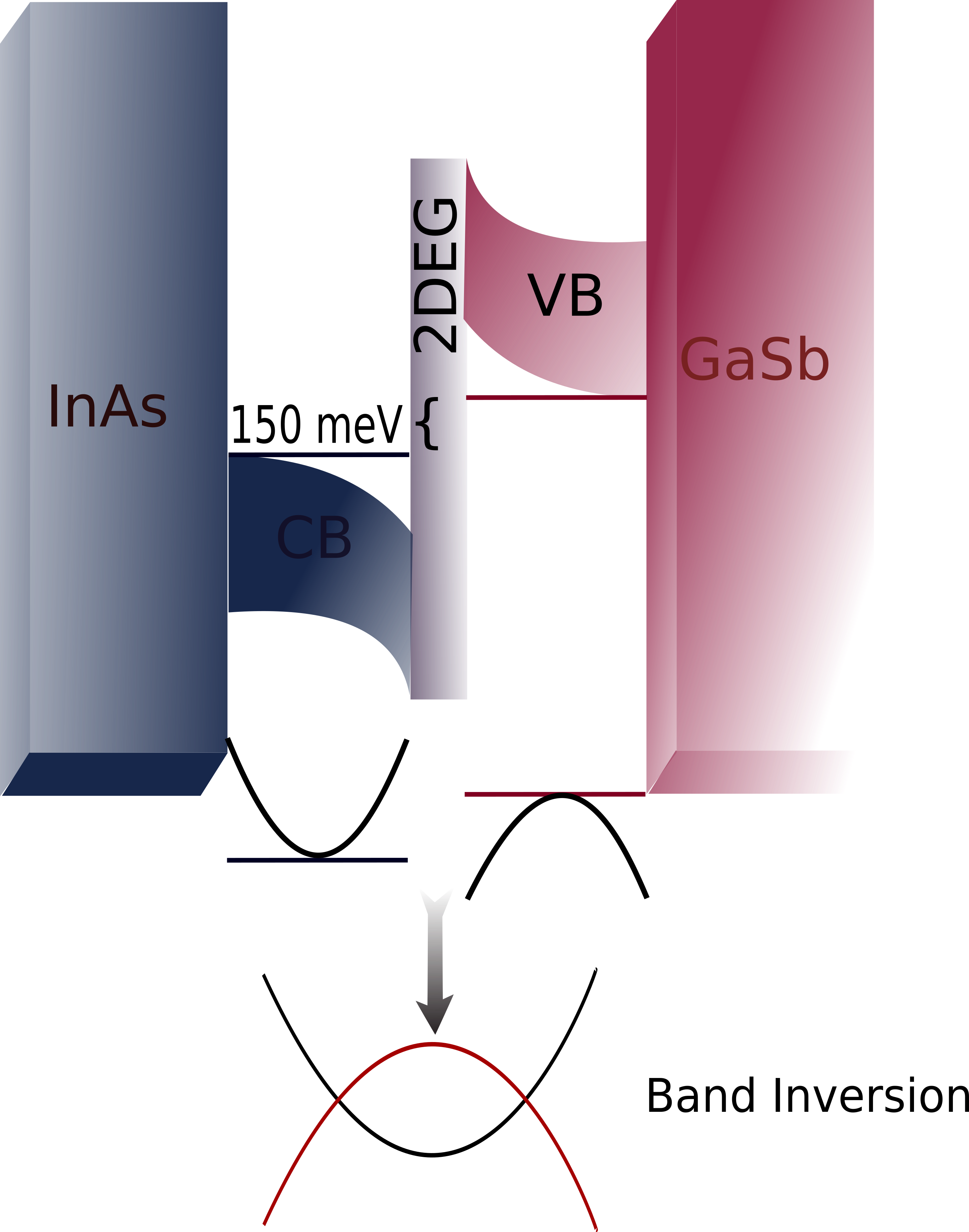
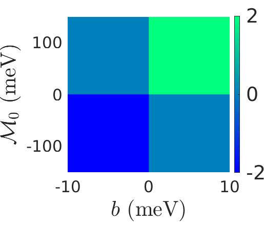
Figure 1: A schematic of the band inversion in the InAs/GaSb bilayer and the topological invariant number in such a bilayer.

$$H=\epsilon({\bf k})\sigma_{0} \mathbin{\mathop{\otimes}}\sigma_{0}+\mathcal{M}({\bf k})\sigma_{0}\mathbin{\mathop{\otimes}}\sigma_{z}+Ak_{x}\sigma_{z}\mathbin{\mathop{\otimes}}\sigma_{x}$$ (1)

$$-Ak_{y}\sigma_{0}\mathbin{\mathop{\otimes}}\sigma_{y}.$$

Here, $\sigma_{i}$, (with $i=x,y,z$) are the Pauli’s spin matrices and $\sigma_{0}$ is the $2\times 2$ identity matrix. The band symmetry-breaking effect between that of the electron and the hole, is captured in the first term $\epsilon({\bf k})=\chi-dk^{2}$. The very important term $\mathcal{M}({\bf k})=\mathcal{M}_{0}-bk^{2}$ has two parameters, viz., ‘$\mathcal{M}_{0}$’ that controls the band inversion and ‘$b$’ that symmetrically controls the band curvatures. The last two terms take care of the finite coupling between the electron and hole states. The BHZ Hamiltonian is governed by the number $\mathcal{C}=({\rm sign}[b]+{\rm sign}[\mathcal{M}_{0}])/2$. This number predicts the existence of the QSH states for a given choice of the set of parameters $\{\mathcal{M}_{0},b\}$.

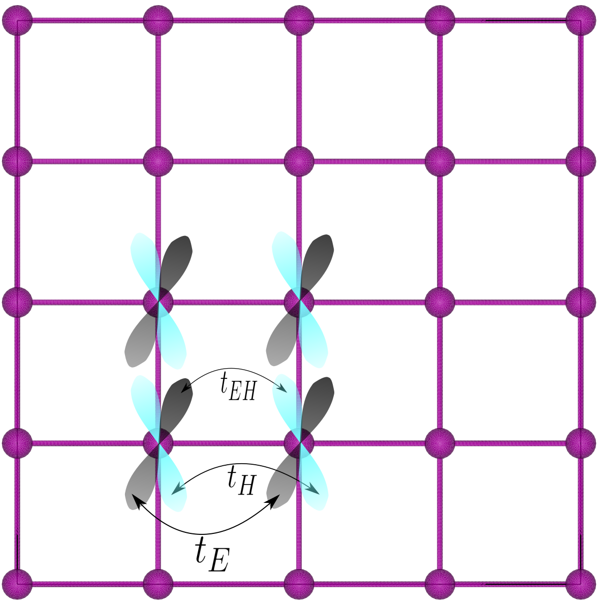
Figure 2: The intra and inter-orbitals hopping between the two orbitals ($E\;\&\;H$) projected on a square lattice for realizing the QSH states in the InAs/GaSb QW. The $E/H$ orbital is illustrated in light black/sky-blue color.

The lattice Model of BHZ Hamiltonian: For realization of the QSH states in such InAs/GaSb QW, we adopt the tight-binding Hamiltonian on a square lattice with two orbitals corresponding to a lattice site (Fig. [2]), represented as $E\;\&\;H$ orbitals. We can think of the two different orbitals to originate from the two III and V elements that give rise to the inverted band structure. The said tight-binding Hamiltonian is written as $H=H_{0}+H_{\mathcal{T}}+H_{\mathcal{Z}},$real_S with

$$\left.\begin{aligned} H_{0}=&\sum_{\textbf{m},\sigma}\big{[}\epsilon_{E}e^{\dagger}_{\textbf{m},\sigma}e_{\textbf{m},\sigma}+\epsilon_{H}h^{\dagger}_{\textbf{m},\sigma}h_{\textbf{m},\sigma}\big{]}\\ H_{\mathcal{T}}=&\sum_{\langle\textbf{m},\textbf{n}\rangle,\sigma}\big{[}t_{E}e^{\dagger}_{\textbf{m},\sigma}e_{\textbf{n},\sigma}+t_{H}h^{\dagger}_{\textbf{m},\sigma}h_{\textbf{n},\sigma}\big{]}+\\ &\sum_{\textbf{m},\sigma}t_{EH}\big{[}s_{z}i\big{(}e^{\dagger}_{\textbf{m},\sigma}h_{\textbf{m}+\hat{x},\sigma}-e^{\dagger}_{\textbf{m},\sigma}h_{\textbf{m}-\hat{x},\sigma}\big{)}\\ &+\big{(}e^{\dagger}_{\textbf{m},\sigma}h_{\textbf{m}+\hat{y},\sigma}-e^{\dagger}_{\textbf{m},\sigma}h_{\textbf{m}-\hat{y},\sigma}\big{)}\big{]}+h.c\\ H_{\mathcal{Z}}&=\sum_{\textbf{m},\sigma}s_{z}\big{[}G_{E}e^{\dagger}_{\textbf{m},\sigma}e_{\textbf{m},\sigma}+G_{H}h^{\dagger}_{\textbf{m},\sigma}h_{\textbf{m},\sigma}\big{]}\end{aligned}\right\}$$ (2)

In the above Hamiltonian, $\epsilon_{E/H}$ denotes the onsite energy of an electron in the $E/H$ orbital. The notation $\langle{\bf m},{\bf n}\rangle$ describes a pair of the nearest neighbor (NN) lattice sites with position vectors ${\bf m}$ and ${\bf n}$. The terms $t_{E/H}$ and $t_{EH}$ denote the energy involed in intra-orbital and inter-orbital hopping, respectively. The magnetic doping we considered is taken into account through the term Zeeman term $H_{\mathcal{Z}}$, with $G_{E/H}$, being the resulting Zeeman energy to the $E/H$ orbital due to the doping at a lattice site. The operators $(e^{\dagger}_{\textbf{m},\sigma}/e_{\textbf{m},\sigma})$ & $(h^{\dagger}_{\textbf{m},\sigma}/h_{\textbf{m},\sigma})$ are the (creation/annihilation) operators for the $E$ and $H$ orbitals, respectively, with spin $\sigma$ at the site ${\bf m}$. Finally, $s_{z}=+/-$ for spin states $\sigma=\uparrow/\downarrow$.

Writing the operator $e_{\textbf{m},\sigma}$ & $h_{\textbf{m},\sigma}$ in terms of the Bloch wavefunction as $e_{\textbf{m},\sigma}=\sum_{\bf k}e_{\textbf{k},\sigma}\exp[i\textbf{k}\cdot\textbf{m}]$ and $h_{\textbf{m},\sigma}=\sum_{\bf k}h_{\textbf{k},\sigma}\exp[i\textbf{k}\cdot\textbf{m}]$, respectively, one can have $H=\sum_{{\bf k}}\psi^{\dagger}_{{\bf k}}H({\bf k})\psi_{{\bf k}}$ where $\psi_{{\bf k}}=\begin{pmatrix}e_{\textbf{k},\uparrow}&h_{\textbf{k},\uparrow}&e_{\textbf{k},\downarrow}&h_{\textbf{k},\downarrow}\end{pmatrix}^{\prime}$ and $H({\bf k})$ is a slightly modified BHZ Hamiltonian as in Eq. [1], with $\mathcal{M}_{0}\rightarrow\mathcal{M}_{0}+8b$ and $\chi\rightarrow\chi+8d$. The parameters $b,\;d,\;\mathcal{M}_{0}$, and $\chi$ in terms of $t_{E},\;t_{H},\;t_{EH},\;\epsilon_{E},\;\epsilon_{H}$ are found to be

$$\left.\begin{aligned} &&b=\frac{t_{E}-t_{H}}{2},\;b=\frac{t_{E}+t_{H}}{2},\;A=-2t_{EH},\\ &&\mathcal{M}_{0}=\frac{\epsilon_{E}-\epsilon_{H}}{2}-2(t_{E}-t_{H}),\\ &&\chi=\frac{\epsilon_{E}+\epsilon_{H}}{2}-2(t_{E}+t_{H})\end{aligned}\right\}$$ (3)

For HgTe, the lattice constant is $a=0.646$ nm. For simplicity, we have taken $a=1$ $A^{\degree}$. For a typical inverted InAs/GaSb QW, the different hopping and onsite energies are $t_{E}=1.74$ meV, $t_{H}=-12$ meV, $t_{EH}=-1.9$ meV, $\epsilon_{E}=17$ meV and $\epsilon_{H}=-58$ meV. Equation [1] allows us to have a set of four energy spin-split bands given by

$$\scalebox{0.91}{\mbox{$\displaystyle E_{\lambda,s_{z}}({\bf k})=\epsilon({\bf k})+s_{z}\frac{G_{E}+G_{H}}{2}+\lambda\sqrt{A^{2}k^{2}+[\mathcal{M}_{s_{z}}(\textbf{k})]^{2}}$}},$$ (4)

with their corresponding eigenstates given by

$$\left.\begin{aligned} &\psi_{{\bf k},\lambda,-1}({\bf r})=\frac{1}{\sqrt{1+{p_{\lambda,-1}({\bf k})}^{2}}}\begin{pmatrix}0\\ 0\\ 1\\ p_{\lambda,-1}({\bf k})\end{pmatrix}\\ &\psi_{{\bf k},\lambda,1}({\bf r})=\frac{1}{\sqrt{1+{p_{\lambda,1}({\bf k})}^{2}}}\begin{pmatrix}1\\ p_{\lambda,1}({\bf k})\\ 0\\ 0\end{pmatrix}\end{aligned}\right\},$$ (5)

where

$$p_{\lambda,s_{z}}({\bf k})=\frac{-s_{z}Ake^{-is_{z}\theta}}{\mathcal{M}_{s_{z}}({\bf k})+\lambda\sqrt{A^{2}k^{2}+\big{[}\mathcal{M}_{s_{z}}({\bf k})\big{]}^{2}}}.$$ (6)

Here, $\mathcal{M}_{s_{z}}({\bf k})=\mathcal{M}({\bf k})+s_{z}\frac{G_{E}-G_{H}}{2}$ and $\lambda=+/-$ which denotes the conduction/valence band.

The two spin-split conduction bands ($\lambda=+$) are characterised by a Berry curvature given by

$$\mathcal{B}_{s_{z}}(\textbf{k})=i\frac{A^{2}\mathcal{M}_{s_{z}}({\bf k})}{2[E_{+,s_{z}}(\textbf{k})-E_{-,s_{z}}(\textbf{k})]^{3}}.$$ (7)

The integral of the Berry curvature over the Brillouin zone, $\mathcal{C}_{s_{z}}=\int{\bf dk}\mathcal{B}_{s_{z}}({\bf k})/2\pi i$ gives the topological invariant number which describes the topological state of the systembook. Thus, here in the case of a magnetic doped QW, we can define two topological invariant number w.r.t. each of the spin states

$$\mathcal{C}_{s_{z}}=\frac{1}{2}\big{[}\text{sign}(b)+\text{sign}\{\mathcal{M}_{0}+8b+s_{z}\frac{G_{E}-G_{H}}{2}\}\big{]}.$$ (8)

The topological state of the system is now defined by the number $\mathcal{C}=\mathcal{C}_{+}+\mathcal{C}_{-}$, which in the undoped case, this number could have values equal to {-2, 0, 2}. The variation of this number as a function of the parameters $\mathcal{M}_{0}$ and $b$ in a magnetic doped QW is shown in Fig. [LABEL:Fig3 a)]. It is now easy for us to separate out three different topological phases as shown in Fig. [LABEL:Fig3 a)]. The QSH phases (with $\mathcal{C}=\pm 2$) host two counterpropagating edge states with opposite spin. When the QW is magnetically doped, we saw a lifting of the Kramer degeneracy as shown in Eqn. (4). With a suitable doping and for some suitable parameters ($\mathcal{M}_{0}\;\&\;b$), the states ($E_{\lambda,-}$), penetrate into the bulk of the materials leaving only the states ($E_{\lambda,+}$) at the edges of the QW. In other words, the system now enters into a QAH topological phase with $\mathcal{C}_{-}=0$ and $\mathcal{C}_{+}=\pm 1$. The QAH phase can also be observed when a strong magnetic field is applied perpendicular to the plane of the QWHamil2; QAH_B1; QAH_B2; QAH_B3; Hamil3; Nat1; QAH_B4. In this case there is no requirement of such strong magnetic field.

Quantum Hall conductivity and Longitudinal conductivity: To have a firm inception of the possibility of the QAH phase, we calculate the static conductivity tensor in a magnetic doped inverted QW, switching off the in-plane magnetic field. Using the Kubo formula in the linear response regime, the transversal conductivity book; ahe in a quantum Hall channel can be written as

$$\sigma_{yx}={\hbar}\lim_{\eta\rightarrow 0}\sum_{\lambda,s_{z}}\int{\bf dk}\frac{f_{\lambda,s_{z}}({\bf k})-f_{-\lambda,s_{z}}({\bf k})}{E_{\lambda,s_{z}}({\bf k})-E_{-\lambda,s_{z}}({\bf k})}$$

$$\times\frac{\mathrm{Im}\,\big{[}\langle\textbf{k},\lambda,s_{z}|\hat{J}_{y}|\textbf{k},-\lambda,s_{z}\rangle\langle\textbf{k},-\lambda,s_{z}|\hat{J}_{x}|\textbf{k},\lambda,s_{z}\rangle\big{]}}{E_{\lambda,s_{z}}({\bf k})-E_{-\lambda,s_{z}}({\bf k})+i\eta}.$$ (9)

Here, the current density operator is written as $\hat{J}_{i}({\bf k})=-e/\hbar\partial_{k_{i}}\hat{H}$ and $f_{\lambda,s_{z}}$ denotes the Fermi-Dirac distribution function for the quantum state $\psi_{\lambda,s_{z}}({\bf k})$. After a fair bid of calculations, we arrive at the following expression for the static Hall conductivity

(10)

To confirm the predicted resistanceless edge states, we also calculate the longitudinal conductivity whose general expression is given as followscalderin

$$\sigma_{xx}=\frac{\beta\hbar}{\pi}\sum_{\lambda,s_{z}}\int{\bf dk}\scalebox{0.94}{\mbox{$\displaystyle f_{\lambda,s_{z}}({\bf k})(f_{\lambda,s_{z}}({\bf k})-1)\delta(E_{\lambda,s_{z}}-E_{\lambda^{\prime},s_{z}^{\prime}})$}}$$

$$\times\mathrm{Re}\,[\langle\lambda,s_{z}({\bf k})|\hat{J}_{x}|\lambda^{\prime},s_{z}^{\prime}({\bf k})\rangle\langle\lambda^{\prime},s_{z}^{\prime}({\bf k})|\hat{J}_{x}|\lambda,s_{z}({\bf k})\rangle].$$ (11)

In this case, this quantity turns out to be

$$\sigma_{xx}=\frac{e^{2}}{\pi\hbar}\frac{\beta}{\Gamma}\sum_{\lambda,s_{z}}\int kdkf_{\lambda,s_{z}}(f_{\lambda,s_{z}}-1)$$

$$\times k^{2}\scalebox{0.94}{\mbox{$\displaystyle\frac{(A^{2}-2b\mathcal{M}_{s_{z}}({\bf k})-\lambda 2d\sqrt{A^{2}k^{2}+[\mathcal{M}_{sz}({\bf k})]^{2}})^{2}}{A^{2}k^{2}+[\mathcal{M}_{sz}({\bf k})]^{2}}$}}.$$ (12)

Results and Discussions: For analysing the results of our calculations, we take the parameters as shown in the table below

$b$ (meV a2)	$d$ (meV a2)	$\chi$ (eV)	$A$ (meV a)	$\mathcal{M}_{0}$ (meV)