A Practical Calibration Method for RGB Micro-Grid Polarimetric Cameras

Abstract

Polarimetric imaging has been applied in a growing number of applications in robotic vision (ex. underwater navigation, glare removal, de-hazing, object classification, and depth estimation). One can find on the market RGB Polarization cameras that can capture both color and polarimetric state of the light in a single snapshot. Due to the sensor’s characteristic dispersion, and the use of lenses, it is crucial to calibrate these types of cameras so as to obtain correct polarization measurements. The calibration methods that have been developed so far are either not adapted to this type of cameras, or they require complex equipment and time consuming experiments in strict setups. In this paper, we propose a new method to overcome the need for complex optical systems to efficiently calibrate these cameras. We show that the proposed calibration method has several advantages such as that any user can easily calibrate the camera using a uniform, linearly polarized light source without any a priori knowledge of its polarization state, and with a limited number of acquisitions. We will make our calibration code publicly available.

I Introduction

In recent years, polarization has started to have more interest in the robotics and computer vision fields [1, 35, 9, 2, 6, 10, 14, 15, 20, 22, 25, 29, 31, 32, 37, 38, 39] . The polarization state of the light is modeled by the Stokes vector with four components that represent the total incoming light intensity and the amount of light that is linearly and circularly polarized. Several types of sensors can be used to measure the polarization state of the light. Among them, the division of focal plane (DoFP) is the most popular and the most suitable for real-time applications since it can measure all the required information to compute the first three Stokes parameters in a single snapshot. It is composed of super-pixels, that are groups of $2\times 2$ pixels, over which are four directional polarizers at an angle of 0^∘, 45^∘, 90^∘ and 135^∘. Sony released a DoFP sensor in 2018, the Polarsens IMX250MYR, that can also measure color information. It is basically an array of four colored super-pixels arranged following a Bayer pattern as represented in Fig. 1 (b).

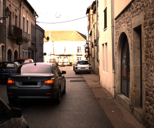
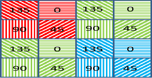
(a)	(b)
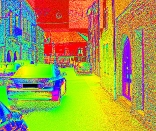
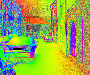
(c)	(d)

Figure 1: Effect of the calibration for measuring the angle of polarization in a real urban scene. (a) Input color image of the scene captured with the RGB polarization camera. (b) The four colored super-pixels of the adopted camera (Sony Polarsens IMX250MYR), arranged following the Bayer pattern with polarizer orientations of $0^{\circ}$, $45^{\circ}$, $90^{\circ}$, and $135^{\circ}$ . (c) Angle of linear polarization image measured with the uncalibrated sensor. (d) Angle of linear polarization image after calibrating the camera with our method. Please notice the differences between (c) and (d), where the angle of polarization of the sky, the building’s roof and front wall in the background were wrongly measured. Without calibration, most of these regions have the same angle of polarization (identified by the same “red” color).

In the Sony Polarsens sensor, the micro-grid polarizers are formed and placed under the layer of micro-lenses used to correctly focus the incoming light onto the pixel, contrary to conventional polarization sensors where it is above the micro-lenses. In this way, the cross-talking effect due to large angle of incidence rays is considerably reduced. Nevertheless, the polarization state determined from the measurement of the light intensities is still inaccurate, as one can notice in the measured angle of polarization of the real urban scene shown in Fig. 1. This is because of the sensor characteristics dispersion due to manufacturing imperfections and to the presence of the lens in front of the camera. The purpose of calibration is to individually correct the outputs of the pixels so that they will all have the same value when the sensor is illuminated with a uniform incident light. Several works attempted to address this calibration problem [4, 12, 23], but the complex experiments for generating the calibration data are time consuming, and require strict experimental setups. In this paper, we describe a practical method to calibrate cameras based on DoFP RGB polarization sensors. It requires only a few samples of a uniform and linearly polarized (ULP) light with moderate values in all of the three RGB channels. The different samples are obtained either by rotating the camera in front of a ULP light source, or by turning a linear polarization filter placed between the camera and an unpolarized light source. Our method will be compared with the well-established super-pixel algorithm, and we show that, although the experimental setup is simpler, our method exhibits similar accuracy. The images of degree of polarization, and angle of polarization will be shown before and after the calibration, concluding that the calibrated pixel’s response is the same over all the sensor area when they are illuminated with a ULP light.

II Related work

Diverse calibration methods have been developed and reported in the literature to correct polarization measurements. However, they are either not suitable for a camera based on an RGB polarization sensor or they require complex equipment, making it hard to replicate the experiments. For example, the method developed by Schechner [26] considers a conventional camera with a polarizer filter in front of it. In this setup, all the pixels share the same polarization filter and thus, to solve the calibration problem, only a few polarized points in a generic scene are needed. This is not the case for a DoFP sensor where each polarization analyzer is composed of four different pixels with polarizers oriented in four different directions. The method by Wang et al.[36] uses an LCD screen to achieve both, polarimetric and geometric calibration of a camera mounted with a polarization filter. Nevertheless, this method cannot be used in our case, because to illuminate all the pixels with the LCD screen, the sensor to the LCD distance must be so short that the pixel pattern of the screen is captured by the camera. Thus, the light cannot be considered uniform. Regarding calibration algorithms dedicated to DoFP sensors, Hagen et al. [12] proposed a method that requires a few samples only, but the angle of polarisation of those samples must be known accurately. Chen [4] introduced a calibration approach that has several constraints in the experiment setup: the light source is expected to come from an integrating sphere, and a band-pass filter is added to estimate the missing pixel through a Fourier-based approach. Moreover, a motorized rotative polarization filter is used, and all the light parameters should be known beforehand. Powell and Gruev [23] calibrate monochrome DoFP polarimeters, by two approaches: the single and super-pixel algorithm. The drawback of their method is that the calibration set up is too elaborated to be replicated, since the light information should be known beforehand. In this paper, a calibration procedure for RGB polarization cameras is presented with the following contributions:

1. A simple and practical pipeline to calibrate ready-to-use polarimetric cameras with a lens, in a single step.

2. A method that does not require any prior knowledge of the polarization state of the calibration light samples. This information is estimated using only a few samples of a ULP light with moderate values for each of the three RGB channels.

3. We demonstrate the effectiveness of the algorithm by showing that only five light samples are enough to calibrate the camera with a good accuracy.

III Pixel model

In this section, the pixel model is briefly described using the Stokes vector and Mueller calculus [27, 8] . The Stokes vector is a convenient way of representing the polarization state of the light. It is composed of four components $\mathbf{\underline{S}}=\left[S_{0},S_{1},S_{2},S_{3}\right]$ where $S_{0}$ is the total intensity of the incident light, $S_{1}$ the amount of linearly polarized light in the horizontal and vertical directions, $S_{2}$ the amount of linearly polarized light in the $\pm 45^{\circ}$ directions, and $S_{3}$ the amount of circularly polarized light.

The calibration method that we have developed are for cameras that are based on DoFP type sensors. These sensors can measure only the linear polarization parameters of the light. So, only linearly polarized light sources or samples will be used to calibrate them. Hence, only the first three components of the Stokes vector are considered. In terms of these three components, the degree of linear polarization (DoLP) and the angle of linear polarization (AoLP), denoted by $\rho$ and $\alpha$, respectively, are defined as follows:

$$\rho=\dfrac{\sqrt{S_{1}^{2}+S_{2}^{2}}}{S_{0}};\ \color[rgb]{0,0,0}{{\alpha=\dfrac{1}{2}\arctan\left(\dfrac{S_{2}}{S_{1}}\right).}}\color[rgb]{0,0,0}$$ (1)

Conversely, representing the Stokes vector components in terms of $\rho$ and $\alpha$ defined in Eq. 1 yields:

$$\mathbf{\underline{S}}=\left[\begin{array}[]{c}S_{0}\\ S_{1}\\ S_{2}\\ \end{array}\right]=\left[\begin{array}[]{c}S_{0}\\ S_{0}\rho\cos\left(2\alpha\right)\\ S_{0}\rho\sin\left(2\alpha\right)\\ \end{array}\right].$$ (2)

Now, let us consider a linearly polarized light that passes through an optical element composed of a pixel of the sensor (with its micro-lens and its micro-polarizer oriented at $\theta^{\circ}$), and the lens of the camera to calibrate. The relationship between the Stokes vector of the input light denoted by $\mathbf{\underline{S}}=\left[S_{0},S_{1},S_{2}\right]^{T}$ and the Stokes vector of the output light denoted by $\mathbf{\underline{O_{out}}}=\left[O_{0\theta},O_{1\theta},O_{2\theta}\right]^{T}$ , is given by:

$$\left[\begin{array}[]{c}O_{0\theta}\\ O_{1\theta}\\ O_{2\theta}\end{array}\right]=\mathbf{M_{u}}\leavevmode\nobreak\ \left[\begin{array}[]{c}S_{0}\\ S_{1}\\ S_{2}\end{array}\right],$$ (3)

where $\mathbf{M_{u}}$ is the Mueller matrix that models all the components in the optical element, i.e., the camera pixel and the lens.

In the output Stokes vector, only the first component $O_{0\theta}$ , that corresponds to the intensity of the light, can be measured by the photosensor device in the pixel. Its expression in terms of the elements of the Mueller matrix $\mathbf{M_{u}}$ [8] is equal to:

$$\color[rgb]{0,0,0}{{O_{0\theta}=\frac{1}{2}\left[q+r\leavevmode\nobreak\ \leavevmode\nobreak\ \left(q-r\right)\cos\text{$\left(2\theta\right)$}\leavevmode\nobreak\ \leavevmode\nobreak\ \left(q-r\right)\sin\text{$\left(2\theta\right)$}\right]\underline{\mathbf{S}}}}\color[rgb]{0,0,0},$$ (4)

where $q$ and $r$ are, respectively, the major and minor light transmittance of the linear polarizer, and $\theta$ the orientation of the micro-filter placed over the pixel [7]. Denoting the intensity measured by the photosensor as $I_{\theta}$, then $O_{0\theta}$ is equal to $I_{\theta}-d_{\theta}$ where $d_{\theta}$ is the dark current noise that must be subtracted from the measured intensity. Also, letting $T=\frac{q-r}{2}$ be the pixel gain, and $P=\frac{\left(q-r\right)}{\left(q+r\right)}$ a coefficient that represents the non-ideality of the filter, Eq. 4 can be rewritten as:

$$\color[rgb]{0,0,0}{{I_{\theta}=\left[\begin{array}[]{ccc}\frac{T}{P}&T\cos\text{$\left(2\theta\right)$}&T\sin\text{$\left(2\theta\right)$}\end{array}\right]\underline{\mathbf{S}}+d_{\theta}.}}\color[rgb]{0,0,0}$$ (5)

In this equation, $d_{\theta}$ is set equal to zero since the dark current can be neglected as it will be shown in the experiment section. So, a pixel with a micro-polarizer at an angle of $\theta^{\circ}$ will be modelled by the following equation:

$$I_{\theta}=\left[\begin{array}[]{ccc}\frac{T}{P}&T\cos\text{$\left(2\theta\right)$}&T\sin\text{$\left(2\theta\right)$}\end{array}\right]\underline{\mathbf{S}},$$ (6)

where $\left(T,P,\theta\right)$ are the pixel parameters. For the super-pixel, as shown in Fig. 1 (b), the measured intensities by the four directional pixels in the $0^{\circ}$, $45^{\circ}$, $90^{\circ}$, $135^{\circ}$ directions can be stacked to give the following equation:

$$\left[\begin{array}[]{c}I_{0}\\ I_{45}\\ I_{90}\\ I_{135}\end{array}\right]=\mathbf{A}\left[\begin{array}[]{c}S_{0}\\ S_{1}\\ S_{2}\end{array}\right],$$ (7)

where $\mathbf{A}$ is the super-pixel matrix, defined as

$$\mathbf{A}=\left[\begin{array}[]{ccc}\nicefrac{{T_{0}}}{{P_{0}}}&T_{0}\cos\left(2\theta_{0}\right)&T_{0}\sin\text{$\left(2\theta_{0}\right)$}\\ \nicefrac{{T_{45}}}{{P_{45}}}&T_{45}\cos\left(2\theta_{45}\right)&T_{45}\sin\text{$\left(2\theta_{45}\right)$}\\ \nicefrac{{T_{90}}}{{P_{90}}}&T_{90}\cos\left(2\theta_{90}\right)&T_{90}\sin\text{$\left(2\theta_{90}\right)$}\\ \nicefrac{{T_{135}}}{{P_{135}}}&T_{135}\cos\left(2\theta_{135}\right)&T_{135}\sin\text{$\left(2\theta_{135}\right)$}\\ \end{array}\right].$$ (8)

In Eq. 8, $\left(T_{i},P_{i},\theta_{i}\right)$ are the parameters of the pixel with micro-filter orientation $i=\left\{0^{\circ},45^{\circ},90^{\circ},135^{\circ}\right\}$. From Mueller calculus theory, ideally, $T_{i}=0.5$ and $P_{i}=1$ for all $i=\left\{0^{\circ},45^{\circ},90^{\circ},135^{\circ}\right\}$, and $\theta_{0^{\circ}}=0^{\circ}$, $\theta_{45^{\circ}}=45^{\circ}$, $\theta_{90^{\circ}}=90^{\circ}$, and $\theta_{135^{\circ}}=135^{\circ}$ for the four pixels of the super-pixel. However, in a real camera with a lens, the true values will deviate from the ideal case. The purpose of our calibration method is to estimate the true value of these parameters for each sensor’s super-pixel.

IV Calibration method

An overview of the pipeline of the proposed method is sketched in Fig. 2. It is grounded on the super-pixel calibration method detailed in [11, 23], which is a well-established method in the literature. The originality of our calibration algorithm is that no information about the input light polarization state is required. Instead, we propose to estimate them and use the estimated polarization state in the calibration method. In Sec. IV-A, the super-pixel calibration method is detailed, in which the input light polarization parameters are required. Then, in Sec. IV-B and Sec. IV-C, we present methods to estimate these light parameters.

IV-A Description of the method

Calibrating a polarimetric camera consists in determining the super-pixel matrix $\mathbf{A}$ of Eq. 8 by solving Eq. 7 for all the super-pixels. To be able to solve this equation that has $\color[rgb]{0,0,0}{{4\cdot 3=12}}\color[rgb]{0,0,0}$ unknowns in the matrix $\mathbf{A}$, at least three calibration light samples must be acquired by the camera. Considering the general case where $N$ calibration samples are acquired with $N\geq 3$, the left hand side intensities vector of Eq. 7 becomes a $4\times N$ matrix, and the Stokes vector becomes a matrix of size $3\times N$. The matricial equation to solve is, thus, defined as:

$$\mathbf{I=AS,}$$ (9)

where $\mathbf{I}$ is the intensity matrix of the $N$ calibration light samples, $\mathbf{A}$ is the super-pixel matrix, and $\mathbf{S}$ is the Stokes vectors matrix of the $N$ calibration light samples. Consequently, using a least-squares approach, the matrix $\mathbf{A}$ is equal to:

$$\mathbf{A=IS^{+},}$$ (10)

where $\mathbf{S}^{+}$ is the pseudo-inverse of S. Eq. 10 constitutes the super-pixel calibration equation, and it can be solved for A if the polarization states of the $N$ input calibration light samples are known . These states corresponds to the $N$ columns of the matrix:

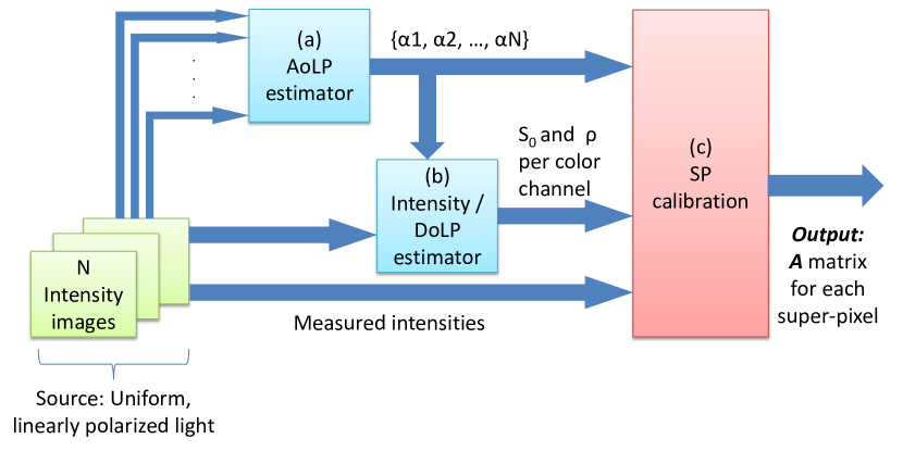
Figure 2: Proposed calibration pipeline. From a uniform linearly polarized light, $N$ samples are captured. The block (a) will estimate the angle of linear polarization of each sample, and with them and the captured images, the block (b) will estimate the degree of linear polarization and the intensity of the source. Finally, with these estimations and the intensity measurements, the super-pixel calibration is done (c).

$$\mathbf{S}=\left[\begin{array}[]{ccc}S_{01}&...&S_{0N}\\ S_{01}\rho_{1}\cos\left(2\alpha_{1}\right)&...&S_{0N}\rho_{N}\cos\left(2\alpha_{N}\right)\\ S_{01}\rho_{1}\sin\left(2\alpha_{1}\right)&...&S_{0N}\rho_{N}\sin\left(2\alpha_{N}\right)\\ \end{array}\right],$$ (11)

where $S_{0n}$ is the intensity of the $n^{th}$ calibration light sample, $\rho_{n}$ is its degree of linear polarization (DoLP), and $\alpha_{n}$ is its angle of linear polarization (AoLP), for $n=1,...,N$. These parameters can be obtained with high accuracy but at the expense of a complex laboratory set-up and time consuming experiments. In the following sections, we will show how to estimate them using a uniform linearly polarized (ULP) light that has moderate values in each of the three RGB channels.

For creating this type of light, two configurations are possible, for which the proposed calibration algorithm is valid: i) a linearly polarized light emitting device is fixed, and the camera is rotated to obtain samples at different angles of linear polarization, or ii) a rotative linear polarization filter is placed between a fixed camera and a fixed unpolarized light source. Due to equipment availability, the second configuration is used for the experiments in this paper.

IV-B Input light angle of polarization estimation

In this section, we describe how to estimate the angles of linear polarization of the $N$ calibration light samples represented by $\alpha_{n}$ with $n=1,...,N$ in Eq. 11. For the visible light wavelengths, the polarization angle measured by a single super-pixel can be considered independent of the color. Furthermore, if the camera is illuminated by a ULP light, all the super-pixels should theoretically observe the same polarization angle. However, this is not the case for a real camera, in general. Due to parameters dispersion, there is not a single pixel in the sensor that can provide an accurate measurement of this angle. Nonetheless, if the mean of the distribution of the AoLP errors is zero, then the mean of all the estimations should be close to the true value.

To compute this mean AoLP, we select a certain number of pixels that are negligibly affected by several undesired effects such as vignetting due to the lens and the aperture, and polarization state errors due to light rays of large angle of incidence. These pixels are those that are found in the central region and that receive light rays pertaining to a small solid angle or Angular Field Of View ($AFOV$). The relationship between the $AFOV$, the length $h$ in $mm$ of a square Region Of Interest (ROI) and the focal length $f$ of the lens in $mm$ is given by

$$AFOV=2\arctan\left(\frac{h}{2f}\right).$$ (12)

Let $p$ be the size of a super-pixel in $mm$ and $AFOV_{max}$ the maximum angular field of view. Eq. 12 can be rearrange to obtain an upper limit for the maximum size of the central region denoted by $N_{sp}$.

$$N_{sp}\leq\left\lfloor\dfrac{h}{p}\right\rfloor=\left\lfloor\dfrac{2f}{p}\tan\left(\dfrac{AFOV_{max}}{2}\right)\right\rfloor$$ (13)

Therefore, any small region of size $N_{sp}\times N_{sp}$ super-pixels around the center that satisfies Eq. 13 for an acceptable angular field of view of about $1^{\circ}$ to $2^{\circ}$ can be considered for estimating the AoLP of the $n^{th}$ light sample using contiguous $2\times 2$ pixels with the same color filter. The measurements will comply with Eq. 7, in which:

• $\color[rgb]{0,0,0}{{\mathbf{\underline{I}}=\left[I_{0}^{j},I_{45}^{j},I_{90}^{j},I_{135}^{j}\right]^{T}}}\color[rgb]{0,0,0}$ is the intensity vector of the $j^{th}$ super-pixel,

• $\color[rgb]{0,0,0}{{\mathbf{\underline{S}}\simeq\mathbf{\hat{\underline{S_{n}}^{j}}}=\left[\hat{S_{n0}^{j}},\hat{S_{n1}^{j}},\hat{S_{n2}^{j}}\right]^{T}}}\color[rgb]{0,0,0}$ is the Stokes vector of the incoming light sample measured by the $j^{th}$ super-pixel,

• $\left(T_{i}^{j},P_{i}^{j},\theta_{i}^{j}\right)$ are the parameters of a pixel that belongs to the super-pixel $j$, and with a micro-polarizer oriented at an angle of $i$ degrees.

For the central pixels, negligible influence of the lens and small sensor artifacts are assumed. Then, the ideal values of $T_{i}^{j}=0.5$, $P_{i}^{j}=1$ for all $i=\left\{0^{\circ},45^{\circ},90^{\circ},135^{\circ}\right\}$ and $\theta=\left\{0{{}^{\circ}},45{{}^{\circ}},90{{}^{\circ}},135{{}^{\circ}}\right\}$ can be adopted as a good approximation. Consequently, the matrix A is completely known, and with its pseudo-inverse, the Stokes vector of the $n^{th}$ light sample, $\mathbf{\hat{\underline{S_{n}}^{j}}}$ can be obtained by:

$$\color[rgb]{0,0,0}{{\mathbf{\hat{\underline{S_{n}}^{j}}}=\left[\begin{array}[]{ccc}\hat{S_{n0}^{j}}&\hat{S_{n1}^{j}}&\hat{S_{n2}^{j}}\\ \end{array}\right]^{T}=\mathbf{A^{+}I}.}}\color[rgb]{0,0,0}$$ (14)

The AoLP $\alpha_{j}$ measured by the super-pixel $j$ is then given by:

$$\color[rgb]{0,0,0}{{\alpha_{j}=\dfrac{1}{2}\arctan\left(\dfrac{\hat{S_{n2}^{j}}}{\hat{S_{n1}^{j}}}\right).}}\color[rgb]{0,0,0}$$ (15)

This operation is repeated for all the $K=N_{sp}\cdot N_{sp}$ super-pixels in the central region. Due to the periodicity of the AoLP, the average of the $K$ angles might conduct to wrong results. Thus, their circular average is computed instead according to Eq. 16. This yields the angle $\hat{\alpha_{n}}$, which is an estimation of the AoLP of the $n^{th}$ light sample denoted by $\alpha_{n}$ with $n=1,...,N$ in Eq. 11.

$$\begin{array}[]{c}\sin\left(2\hat{\alpha_{n}}\right)=\frac{1}{K}\sum_{j=1}^{K}\sin\left(2\alpha_{j}\right)\\ \cos\left(2\hat{\alpha_{n}}\right)=\frac{1}{K}\sum_{j=1}^{K}\cos\left(2\alpha_{j}\right)\\ \hat{\alpha_{n}}=\frac{1}{2}\arctan\left(\sin\left(2\hat{\alpha_{n}}\right)/\cos\left(2\hat{\alpha_{n}}\right)\right)\end{array}$$ (16)

IV-C Light samples intensity and DoLP estimation

We will now describe how to estimate the light intensities and the DoLP of the $N$ calibration light samples defined in the matrix $\mathbf{S}$ of Eq. 11.

For the same reasons as explained in Sec. IV-B, a $N_{sp}\times N_{sp}$ super-pixels region around the center of the sensor is considered for all the light samples that will have the same intensity and the same DoLP. Only the AoLP will be different by selecting a different orientation of the rotative filter for each sample. Thus, in Eq. 11, $S_{01}=...=S_{0N}=S_{0}$ and $\rho_{1}=...=\rho_{N}=\rho$. Consequently, the Stokes matrix of the $N$ calibration light samples S can be split into two matrices: a $3\times 3$ matrix L that only depends on $\left(S_{0},\rho\right)$, and a $3\times N$ matrix G that only depends on the angles of linear polarization $\alpha_{n}$ estimated in Sec. IV-B, such that $\mathbf{S=LG}$:

$$\begin{array}[]{c}\mathbf{S}=\left[\begin{array}[]{ccc}S_{0}&0&0\\ 0&S_{0}\rho&0\\ 0&0&S_{0}\rho\\ \end{array}\right]\left[\begin{array}[]{ccc}1&...&1\\ \cos\left(2\alpha_{1}\right)&...&\cos\left(2\alpha_{N}\right)\\ \sin\left(2\alpha_{1}\right)&...&\sin\left(2\alpha_{N}\right)\\ \end{array}\right]\\ \\ \end{array}$$ (17)

Combining Eq. 9, which is the super-pixel calibration equation, and Eq. 17, yields:

$$\mathbf{IG^{+}=AL,}$$ (18)

where I is the $4\times N$ matrix of the measured intensities. For the super-pixel $j$, each row $i$ of the result $\mathbf{IG^{+}}$ can be expressed as:

$$\left(\mathbf{IG^{+}}\right)_{i}^{j}=\left[\begin{array}[]{ccc}X_{i}^{j}&Y_{i}^{j}&Z_{i}^{j}\end{array}\right],$$ (19)

where $X_{i}^{j}=\frac{T_{i}^{j}S_{0_{i}}^{j}}{P_{i}^{j}}$, $Y_{i}^{j}=T_{i}^{j}S_{0_{i}}^{j}\rho_{i}^{j}\cos\left(2\theta_{i}^{j}\right)$, and $Z_{i}^{j}=T_{i}^{j}S_{0_{i}}^{j}\rho_{i}^{j}\sin\left(2\theta_{i}^{j}\right)$. If the camera is considered ideal for the central pixels, as in the previous section, each of the four rows of $\mathbf{IG^{+}}$ allows to calculate a pair $\left(S_{0_{i}}^{j},\rho_{i}^{j}\right)$ as follows:

$$\begin{array}[]{cc}S_{0_{i}}^{j}=2X_{i}^{j}&\rho_{i}^{j}=\dfrac{\sqrt{Y_{i}^{j2}+Z_{i}^{j2}}}{X_{i}^{j}}.\end{array}$$ (20)

Repeating this procedure for the $K$ super-pixels and the $N$ samples will yield two sets of $R=N_{sp}\cdot N_{sp}\cdot 4$ intensities and DoLP: $\left\{S_{0}^{1},S_{0}^{2},...,S_{0}^{R}\right\}$ and $\left\{\rho^{1},\rho^{2},...,\rho^{R}\right\}$. From these two sets, the light parameters, $S_{0}$ and $\rho$, can be estimated by extracting either the maximum (highly sensitive to noise and outliers), the average (affected by lens vignetting and outliers) or the median (affected only by lens vignetting) value. Because of its robustness to outliers, the median value has been chosen and implemented for the experiments.

It is important to note that a color camera is used. To be free from the requirement of using a white light, the detected intensities and DoLP have to be classified per color channel, without mixing them. The color channel to which a super-pixel belongs to is given by its position $j$.

At this point, an estimation of the light intensity $\hat{S_{0}}$, the degree of linear polarization $\hat{\rho}$ per color channel, and the angle of polarization $\hat{\alpha_{n}}$ at the $n^{th}$ position of the linear filter has been obtained. Therefore, the Stokes matrix can be built, as in Eq. 21,

$$\hat{\mathbf{S}}=\left[\begin{array}[]{ccc}\hat{S_{0}}&0&0\\ 0&\hat{S_{0}}\hat{\rho}&0\\ 0&0&\hat{S_{0}}\hat{\rho}\\ \end{array}\right]\left[\begin{array}[]{ccc}1&...&1\\ \cos\left(\hat{\alpha_{1}}\right)&...&\cos\left(\hat{\alpha_{N}}\right)\\ \sin\left(\hat{\alpha_{1}}\right)&...&\sin\left(\hat{\alpha_{N}}\right)\\ \end{array}\right].$$ (21)

and its pseudo-inverse $\hat{\mathbf{S}}^{+}$ computed and used in Eq. 10 to calculate the $j^{th}$ super-pixel matrix that we will denote here by $\hat{\mathbf{A_{j}}}$. It follows that, from $\hat{\mathbf{A_{j}}}$, each row allows to compute the parameters $\left(T_{i},P_{i},\theta_{i}\right)$ for each of the four pixels that compose the $j^{th}$ super-pixel.

V Experiments

Our experimental setup is composed of a Basler acA2440-75ucPOL camera with a Sony Polarsens IMX250MYR sensor of pixel size equal to $3.45\mu m$ or super-pixel size equal to $6.9\mu m$, and a Fuji-film HF16XA-5M - F1.6/16mm lens. To compute an initial estimation of the AoLP and DoLP required by our calibration method, we have chosen a central region of $50\times 50$ super-pixels determined according to Eq. 13. This region corresponds to incident light rays with a maximum angle of incidence of $0.625^{\circ}$ that is relatively small and will give a good initial estimation of the AoLP and DoLP.

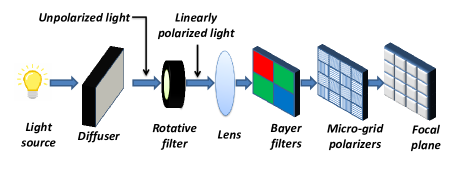
Figure 3: The experiment set up where only one super-pixel is represented.

The developed algorithm runs on a computer with Intel Core i7-10850H @ 2.7 GHz and 32 GB of RAM. The OS is Ubuntu 18.04 LTS 64 bits. The program runs in 7 seconds for 7 samples, and 8 seconds for 73 samples approximately. The experimental set-up model is shown in Fig. 3. The uniform, unpolarized light source device is a Schott Fostec DCR III fiber optic illuminator, with a Schott ColdVision back light A08927. A 50mm linear glass polarizing filter is used (Edmund Optics Inc #56-329), mounted on a metric polarizer mount (Edmund Optics Inc #43-787). The linear polarizer filter is rotated by hand. Each position of the filter corresponds to a light sample, and for each sample ten acquisitions of the light are done and averaged to reduce the effects of the noise in the parameters estimation. The acquisitions are done in a dark room to reduce the influence of the environment. Furthermore, the recommendations given in [17] have been followed. Particularly, the lens has been correctly focused at the light source, and the $f$-number has been set higher than 2.8 for all the experiments. Finally, we have acquired several images with the camera in total darkness and verified that, with a 12-bit pixel count and an exposure time of 1s, the dark current can effectively be neglected as reported in [17].

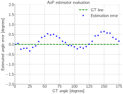
Figure 4: AoLP estimator evaluation. The maximum error is of $0.65^{\circ}$, and the RMSE is of $0.3316^{\circ}$ for all the range from $\left[0^{\circ},180^{\circ}\right]$. The sine-like evolution is mainly due to the error in the polarizers orientations [24].

The first experiment that we have done is to verify the quality of the estimated AoLP with the camera. To do so, different light samples with different AoLP have been used. The AoLP values are set by turning the polarization filter in front of the light source by steps of $5^{\circ}$, in the range $\left[0^{\circ},175^{\circ}\right]$. Thirty-six images of the source light samples are acquired with the camera, and from them the AoLP are calculated and compared to the true reference values given by the position of the polarization filter. For better visualization, only the deviations from the reference values are represented in Fig. 4. In case the estimated AoLP values are the same as the reference values, an horizontal line at zero degree is obtained. However, in our case, the AoLP error curve exhibits a sine-like shape that is due to errors in the parameters of the camera. Indeed, it can be proven that a small error in the parameters of the camera due to imperfections will induce, in first order approximations, four error terms in the expression of the estimated AoLP. These error terms are functions of the sine and cosine of the true AoLP and they appear in the expressions of the computed Stokes components $S_{1}$ and $S_{2}$. Because of these additional components, and that the ratio of these two Stokes components is proportional to the tangent of the AoLP (Eq. 1), the error curve follows a sine and cosine rule. The detailed demonstration of this effect can be found in the supplementary material [24] (it is not included in the main paper since it is an auxiliary result of this work, and also due to space constraints). Nonetheless, by considering pixels around the center, and averaging several samples, the estimation error is reduced, such that the RMSE is $0.3316^{\circ}$, and the maximum error is $\pm 0.65^{\circ}$ in all the range. Hence, the experiment confirms that the camera can be used to provide reliable measurements of the AoLP of the ULP light. Additionally, it avoids the requirement of aligning the rotative filter and the camera, since the measurements are already in the camera’s coordinate frame.

The next step is to evaluate the accuracy of the calculated intensities, AoLP and DoLP with the uncalibrated and the calibrated camera with $N$ number of calibration light samples. Prior to the test, a database has been created with all the images of the required calibration light samples. These samples have the same intensity and DoLP, but different AoLP in the range of $\left[0^{\circ},180^{\circ}\right]$. For the test, $N$ sample images are randomly selected from the database and used to compute the pixel parameters. Once the camera is calibrated, the intensity, DoLP and AoLP of a test image are calculated. The mean and standard deviation of the test light parameters are calculated over all the sensor area. This test is repeated several times for each value of $N=3,...,36$. For each run of the algorithm, a new set of $N$ random calibration images is chosen to calibrate the camera. The GT values of the test image are: $S_{0}=1437$, $\rho=0.97$, and $\alpha=43{{}^{\circ}}$. For space reasons, only the results for the red channel are shown in Fig. 5. Those for the other channels can be found in the supplementary material [24].

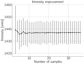
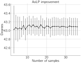
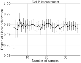
(a)	(b)	(c)

Figure 5: Comparative graphs of how the accuracy changes with the number of light samples. Each sample is taken at a different position of the rotative filter. Each point in the curve is the average of several runs of the algorithm. The black curves are the mean values, and the gray vertical bars are the standard deviation. When uncalibrated, the parameters are: $S_{0}=1336.327\pm 61.731$, $\rho=0,9776\pm 0,006$, and $\alpha=43,024^{\circ}\pm 0.48^{\circ}$. When calibrated and the amount of samples $N\geq 10$, $S_{0}=1437.134\pm 9.25$, $\rho=0.98\pm 0.005$ and $\alpha=43.099^{\circ}\pm 0.2^{\circ}$. (a) Intensity $S_{0}$. (b) AoLP $\alpha$. (c) DoLP $\rho$.

As shown in Fig. 5, when five or more calibration light samples are used, the standard deviation is considerably reduced with respect to the case when only three samples are used, and when $N\geq 10$, the values are stabilized. More precisely, for $N\geq 10$, $S_{0}=1437.134\pm 9.25$, $\rho=0.98\pm 0.005$ and $\alpha=43.099^{\circ}\pm 0.2^{\circ}$. The same test image has been used with the uncalibrated camera , and the obtained parameters were: $S_{0}=1336.327\pm 61.731$, $\rho=0,9776\pm 0,006$, and $\alpha=43,024^{\circ}\pm 0.48^{\circ}$. This experiment also corroborates that the camera calibrated with our algorithm reduces the disparity between values over the sensor area with respect to the uncalibrated camera.

To confirm the validity of our method with respect to other algorithms, the calibration results have been compared with the super-pixel (SP) method described in [11, 23]. Tab. I summarizes the comparison results. The AoLP used for the SP method has been measured from the rotative filter, while for our method they have been estimated. The difference between the mean values of the intensity and the DoLP is expected, since each method uses a different reference during calibration. However, the most important results are the standard deviations that reflect how similar the measurements of the ULP light are after the correction over the entire sensor area. One can notice that the results obtained by both approaches have similar accuracy. However, our method has the advantage of being experimentally simple: it does not require any specific devices to measure the light polarization state. Additionally, the time required to take the samples is reduced for the user since he only needs to randomly turn the polarizer a few times. Also, the measurements of the orientation from the rotative filter are not required since the algorithm will estimate them automatically.

	$S_{0}$	$AoLP$	$DoLP$
Uncalibrated	3399.2 [65.475]	59.983 [0.215]	0.9863 [0.0041]
SP method	3402.4 [10.723]	60.035 [0.128]	1.005 [0.004]
Our method	3298.0 [10.402]	59.701 [0.128]	0.985 [0.004]

TABLE I: Comparison of our method with the super-pixel (SP) method [11]. Content of each cell: mean value [standard deviation]

Finally, the effect of calibration on an image of a ULP light is presented in Fig. 6. For space reasons, only the results for the red channel are shown. The results for the other channels are available in [24]. In this figure, the images (a) and (b) corresponds to AoLP image, before and after calibration, and the images (c) and (d) are the corresponding images of the DoLP. These images are the measurements of the camera when it is illuminated by a ULP light. For the uncalibrated case, the values of the AoLP and the DoLP are in the intervals $\left[0.9465,1.0\right]$, and $\left[41.099^{\circ},44.879^{\circ}\right]$, respectively. For the calibrated camera the corresponding values are in the intervals $\left[0.9741,1.0\right]$, and $\left[41.934^{\circ},43.824^{\circ}\right]$, respectively. What is important to note in these images is not the color but the variations in the colors. Since, these images represent the values of the measured AoLP and DoLP, by the individual pixels of the camera, they should respectively be the same, i.e. all the pixels of the same image should have the same color, due to the fact that the observed light is uniform and linearly polarized. However, this is not the case. The variations in the color represent the measurement errors by the individual pixels. One can note that the color is more uniform (and therefore, there is less errors) for the calibrated camera than for the uncalibrated camera.

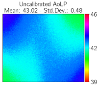
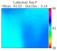
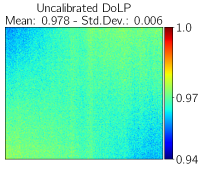
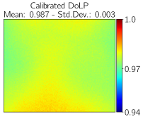
(a)	(b)	(c)	(d)

Figure 6: Calibration improvement image for the red channel. (a) Uncalibrated AoLP image (b) Calibrated AoLP image. (c) Uncalibrated DoLP image. (d) Calibrated DoLP. AoLP uses the HSV color palette, and the DoLP uses the Jet palette. Since the light source is ULP, the ideal response would be images with a single value for all the pixels for the AoLP and another value for the DoLP. Due to characteristics dispersion in the pixels and the presence of the lens, the uncalibrated images present different values between the center of the sensor and its borders in the two polarization parameters. After calibration, the distribution of measured values is reduced. Even though there seems to be a difference in the colors of the calibrated images, looking at the color bars range, it is clear that the range of values present in the image is small compared to the uncalibrated cases. Additionally, the mean and the standard deviation of values in the images are detailed in the images titles.

Additionally, these images show that, for the uncalibrated images, both polarization parameters present changes in the borders with respect to the center of the image. This is a consequence of the lens vignetting. Indeed, the variation of the polarization state of the incoming light depends on the point of incidence of the light at the lens surface. As one can see in Fig. 6, the uncalibrated measurements have strong variations in the four corners of the images, and in the center they are mostly constant. This effect is equivalent to having a Mueller matrix applied to the input light, where this matrix is different at each lens point. The proposed algorithm accounts for this alteration of the polarization state in the pixel model, by modulating the polarizers parameters $P_{i}$ and $\theta_{i}$, to fit the measurements with a flat-field response. $T_{i}$ has no effect over these parameters since it is a factor of all the three Stokes parameters, thus it is cancelled when computing the DoLP and the AoLP. However, $T_{i}$ corrects the vignetting effect over the intensity image, which has not been included here due to space restrictions, but it can be found in the supplementary material [24].

Ablation study. To test the influence of each module, several scenarios have been evaluated and summarized in Tab. II. The first row of this table, SC1, corresponds to the results when using the uncalibrated camera. Then, in SC2, the AoLP estimator has been used and the DoLP and intensity of the input light have been fixed to 0.8 and 2000, respectively. As shown in the table, this modification changes the corresponding mean value measured in the entire image, but their standard deviation (SD) is not modified. The advantage of having a module that estimates these parameters is that an early saturation of the measured value is avoided. Then, in SC3, the AoLP estimator is disabled, and these values have been measured from the filter ruler. In this case, the AoLP after calibration presents a slightly smaller SD than when using the estimator, due to the small error in the measurements of this parameter. Nonetheless, this has as trade off a large experiment time, and the requirement of a rotative mount with a ruler. In SC4, a similar experiment to SC3 is done, but a fixed shift is introduced in the AoLP measurements. From Tab. II it can be seen that this affects the mean value of the measured AoLP, but the SD remains low. This is normal, since the AoLP is relative to the measurement system. Finally, our entire pipeline is tested in SC5, in which a small SD is obtained in all the variables, and additionally, the mean values are close to the GT values. Therefore, using a simple calibration set-up as ours can provide not only accuracy, but also precision in the measurements given by the camera.

	$S_{0}$ $\left[0,4095\right]$	$AoLP$ (∘)	$DoLP$ $\left[0,1\right]$
SC1	2750.66 [153.46]	60.08 [0.416]	0.986 [0.0033]
SC2	1985.63 [4.88]	59.87 [0.126]	0.797 [0.00362]
SC3	2967.34 [7.24]	59.61 [0.125]	0.987 [0.0045]
SC4	2967.38 [7.24]	69.61 [0.125]	0.978 [0.0044]
SC5	2969.6 [7.26]	59.87 [0.126]	0.973 [0.0044]

TABLE II: Results of the ablation experiments.

Applications. The proposed calibration can be applied to improve different applications such as shape-from-polarization and monocular depth estimation. Particularly, surface reconstruction from polarization applications are often affected by discontinuities in the estimated surfaces due to the accumulated error in the normal’s integration. Notably, these errors are linked to the error in the estimation of the AoLP and the DoLP (due to the pixel’s parameters dispersion), which are reduced by the proposed calibration approach.

An example of robotics application is given in Fig. 7, in which a parabolic shaped piece surface is retrieved by using the SfP technique explained in [30]. In this image, the highlighted error is due to the error in the normal’s vector field integration. This accumulated error makes that the point where the end of the surface meets the beginning will not match, producing the discontinuity shown. This reconstruction error is reduced when using the calibrated camera (highlighted area). Although a detailed analysis of applications are out of the scope of this paper, we are providing some reconstruction results with two recent 3D shape estimation approaches in the supplementary material.

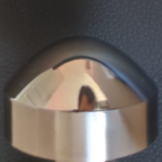
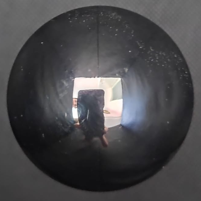
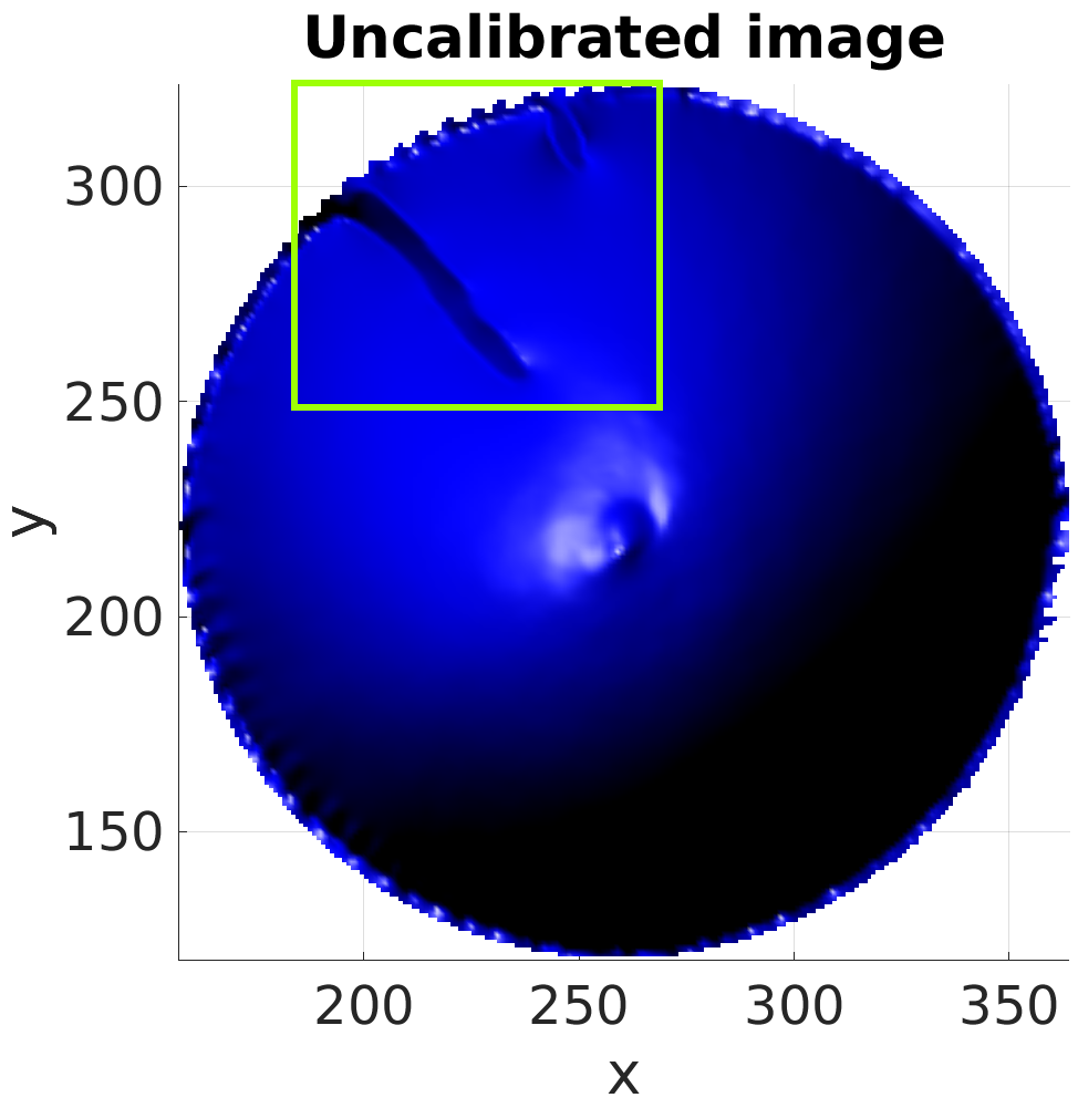
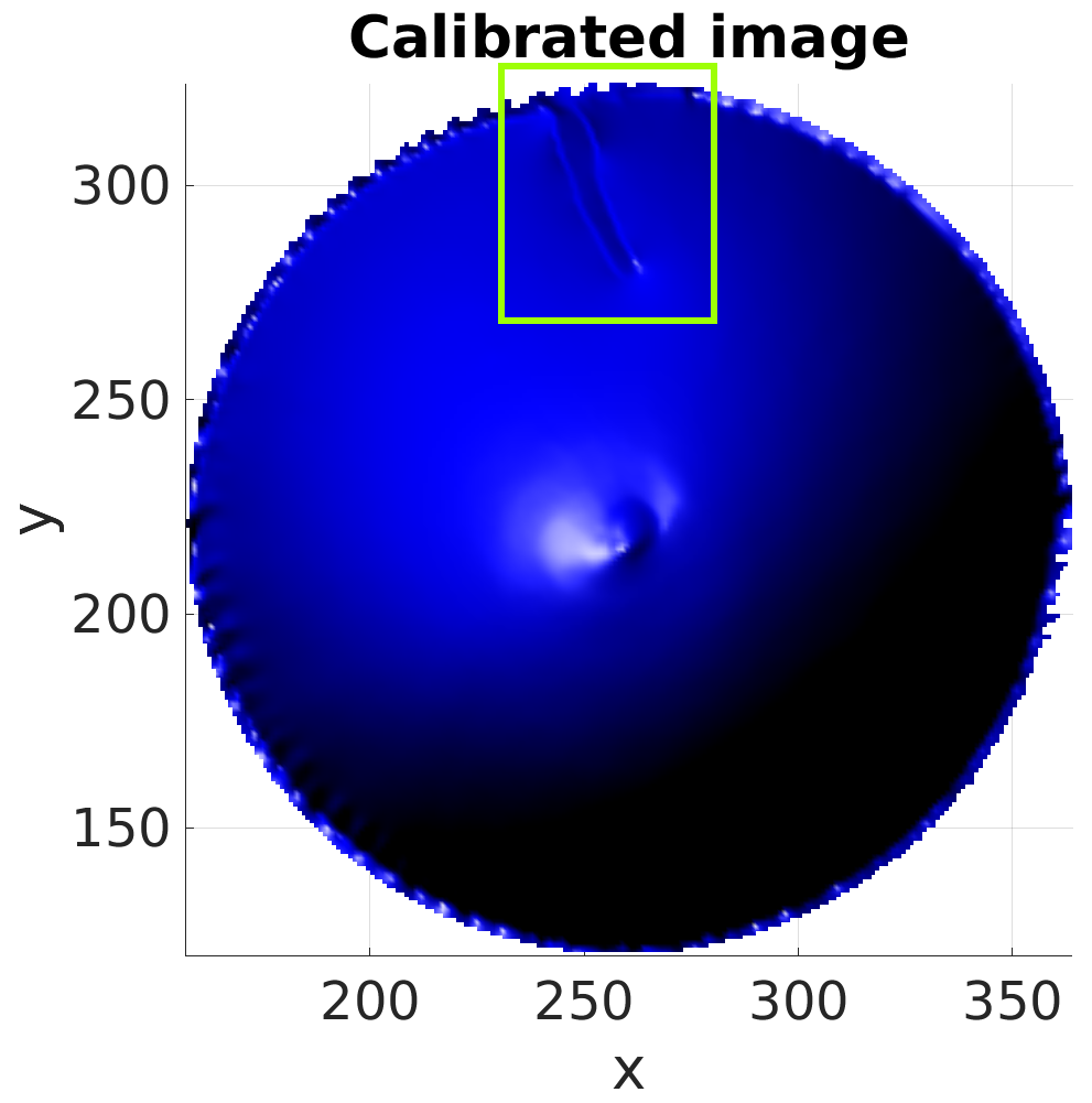
(a)	(b)	(c)	(d)

Figure 7: 3D reconstruction application with Shape-from-Polarization method [30]. (a) Original piece - front view. (b) Original piece - top view. (c) 3D reconstruction top view of the piece with the uncalibrated camera. (d) 3D reconstruction top view of the piece with the calibrated camera.

VI Conclusions

A calibration algorithm for RGB micro-grid polarization cameras has been presented. The developed framework is flexible to be extended to any amount of light samples. We show that with a minimal set-up, and without any knowledge about the source light polarization state, the calibration problem can be solved by using the light parameters estimators included in this work. Five image samples is the minimum requirement to highly increase the camera estimation accuracy. The calibration light samples must be uniform and linearly polarized, at different AoLP. Since each color channel is considered independently from the others, the light source is not restricted to be white, but it should have a certain value in each color frequency. All the results in this paper have been validated with experiments, showing that the algorithm performance is competitive to recent calibration techniques.

Supplementary material

This is the supplementary material of our RAL 2022 submission entitled “A practical calibration method for RGB micro-grid polarimetric cameras”. This document includes additional demonstrations and experiments that might be of interest to the readers.

Appendix A: Sine-like shape of the AoLP estimator error

In this appendix, we demonstrate why the error of the AoLP estimator has a sine-like shape. This demonstration is auxiliary to the submitted paper and the explanation was not included in the main paper due to space restrictions. The shape shown in Fig. 8 is a plot of the error in the circular average of the angle of linear polarization. The estimated angle is calculated from the intensity measurements of a $50\times 50$ region around the center of the sensor with a 16mm lens. For each AoLP, ten images of a uniform, linearly polarized light are captured and averaged to reduce the influence of the noise in the estimations.

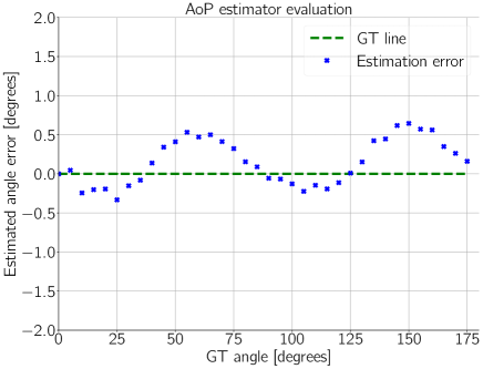
Figure 8: AoLP estimator error plot.

VII Demonstration

When a pixel and its polarization filter are not ideal, the relationship between the Stokes vector and its measured intensity is given by Eq. (6) in the main paper:

$$I_{i}=T_{i}\left[\begin{array}[]{ccc}\dfrac{1}{P_{i}}&\cos\left(2\theta_{i}\right)&\sin\left(2\theta_{i}\right)\\ \end{array}\right]\left[\begin{array}[]{c}S_{0}\\ S_{1}\\ S_{2}\\ \end{array}\right],$$ (22)

where $I_{i}$ is the measured pixel intensity, $T_{i}$ is the pixel gain, $P_{i}$ is a factor that models the non-ideality of the pixel micro-filter, and $\theta_{i}$ is the micro-filter orientation, for $i=\left\{0^{\circ},45^{\circ},90^{\circ},135^{\circ}\right\}$.

To demonstrate the error equation in the estimated AoLP, we compute the error in the measured Stokes components when the pixels are considered ideal.

$$\begin{array}[]{c}\hat{S_{1}}=I_{0}-I_{90}\\ \hat{S_{2}}=I_{45}-I_{135}\\ \end{array}$$ (23)

Considering the pixel model of Eq. 22, and assuming that the micro-filter with orientation $i$ has an error $\varDelta\theta_{i}$ with respect to its ideal orientation, we obtain:

$$\small\begin{array}[]{c}\hat{S_{1}}=\left[T_{0}\left[\begin{array}[]{ccc}\dfrac{1}{P_{0}}&\cos\left(2\varDelta\theta_{0}\right)&\sin\left(2\varDelta\theta_{0}\right)\end{array}\right]\right.-\\ \left.{T_{90}\left[\begin{array}[]{ccc}\dfrac{1}{P_{90}}&\cos\left(\pi+2\varDelta\theta_{90}\right)&\sin\left(\pi+2\varDelta\theta_{90}\right)\end{array}\right]}\right]\left[\begin{array}[]{c}S_{0}\\ S_{1}\\ S_{2}\end{array}\right]\end{array}$$ (24)

Using the sine and cosine properties, and grouping terms gives:

$$\hat{S_{1}}=\left[\begin{array}[]{ccc}A&B&C\\ \end{array}\right]\left[\begin{array}[]{c}S_{0}\\ S_{1}\\ S_{2}\\ \end{array}\right],$$ (25)

with

$$\begin{array}[]{c}A=\dfrac{T_{0}}{P_{0}}-\dfrac{T_{90}}{P_{90}}\\ \\ B=T_{0}\cos\left(2\varDelta\theta_{0}\right)+T_{90}\cos\left(2\varDelta\theta_{90}\right)\\ \\ C=T_{0}\sin\left(2\varDelta\theta_{0}\right)+T_{90}\sin\left(2\varDelta\theta_{90}\right)\\ \end{array}$$

Since the angle error can be considered close to zero, then the corresponding Taylor expansions up to order two can be used to replace the sine and cosine functions. Moreover, by doing the matricial multiplication we obtain:

$$\begin{array}[]{c}\hat{S_{1}}=AS_{0}+\left[T_{0}+T_{90}-2T_{0}\varDelta\theta_{0}^{2}-2T_{90}\varDelta\theta_{90}^{2}\right]S_{1}+\\ \\ \left[2T_{0}\varDelta\theta_{0}+2T_{90}\varDelta\theta_{90}\right]S_{2}.\\ \end{array}$$ (26)

If the angle errors are between $\left[-10^{\circ},10^{\circ}\right]$, the corresponding range in radians is $\left[-0.1745,0.1745\right]$. Thus, if we square this range, we obtain a range of values $\left[0,0.03\right]$. The orientation errors due to manufacturing problems have values less than $10^{\circ}$, therefore, the second order variables can be ignored, i.e.:

$$\hat{S_{1}}=AS_{0}+G^{{}^{\prime}}S_{1}+K_{1}S_{2}.\\$$ (27)

with:

$$\begin{array}[]{c}G^{{}^{\prime}}=T_{0}+T_{90}\\ \\ K_{1}=2T_{0}\varDelta\theta_{0}+2T_{90}\varDelta\theta_{90}.\end{array}$$

Similarly, $\hat{S_{2}}$ can be obtained as a function of the Stokes components.

$$\hat{S_{2}}=DS_{0}-K_{2}S_{1}+G^{{}^{\prime\prime}}S_{2}.\\$$ (28)

where:

$$\begin{array}[]{c}D=\dfrac{T_{45}}{P_{45}}-\dfrac{T_{135}}{P_{135}}\\ \\ G^{{}^{\prime\prime}}=T_{45}+T_{135}\\ \\ K_{2}=2T_{45}\varDelta\theta_{45}+2T_{135}\varDelta\theta_{135}.\end{array}$$

It follows that the estimated AoLP $\hat{\alpha}$ is equal to:

$$\hat{\alpha}=\dfrac{1}{2}\arctan\left(\dfrac{\hat{S_{2}}}{\hat{S_{1}}}\right)=\dfrac{1}{2}\arctan\left(\dfrac{DS_{0}-K_{2}S_{1}+G^{{}^{\prime\prime}}S_{2}}{AS_{0}+G^{{}^{\prime}}S_{1}+K_{1}S_{2}}\right)$$ (29)

Remembering that $S_{1}=S_{0}\rho\cos\left(2\alpha\right)$, and $S_{2}=S_{0}\rho\sin\left(2\alpha\right)$, where $\rho$ is the degree of linear polarization, and $\alpha$ is the angle of linear polarization of the incoming light, Eq. 29 becomes:

$$\hat{\alpha}=\dfrac{1}{2}\arctan\left(\dfrac{D-K_{2}\rho\cos\left(2\alpha\right)+G^{{}^{\prime\prime}}\rho\sin\left(2\alpha\right)}{A+G^{{}^{\prime}}\rho\cos\left(2\alpha\right)+K_{1}\rho\sin\left(2\alpha\right)}\right)\\$$ (30)

This equation converges to the true AoLP $\alpha$ if the pixels and the filters are ideal, i.e., $P_{i}=1$, $T_{i}=0.5$, and $\varDelta\theta_{i}=0$, for $i=\left\{0,45,90,135\right\}$. In a real case, slight deviations from these values will appear. The sources of these deviations are the manufacturing process of the sensor, and the lens added to the camera. As mentioned in the main paper, considering a small region around the center of the sensor reduces the deviations caused by the lens.

Analyzing this equation, it is possible to conclude that:

• The deviations in the pixel parameters will make the other Stokes parameters to influence the AoLP measurement.

• The deviations in the orientations of the micro-polarizers, denoted by $\varDelta\theta_{i}$, for $i=\left\{0,45,90,135\right\}$ will introduce an error based on the value of the complementary Stokes parameter (for the measurement of $S_{1}$, a deviation in the orientation of the micro-polarizers will introduce an error based on the value of $S_{2}$, and an error based on $S_{1}$ in the measurement of $S_{2}$).

• For measurements of the same light at different AoLP, the deviations in the non-ideality factor $P_{i}$ and the gain $T_{i}$ will produce a constant shift in both, numerator and denominator, of Eq. 30.

• The values of $K_{1}$ and $K_{2}$ should be close to zero, and this can happen in two situations: either the pixel parameters are almost ideal and therefore the orientation errors are almost zero, or the pixels orientation error are almost the same, but in opposite directions. The second case can be understood by looking at the definitions of these variables. For instance, $K_{1}=2T_{0}\varDelta\theta_{0}+2T_{90}\varDelta\theta_{90}$, where $T_{0}$ and $T_{90}$ are positive numbers, and in general, they are close to $0.5$. Therefore, if $\varDelta\theta_{0}\simeq-\varDelta\theta_{90}$, then $K_{1}$ will have a very tiny value. Similarly, $K_{2}$ will be almost zero when $\varDelta\theta_{45}\simeq-\varDelta\theta_{135}$. Finally, it can be seen that the errors in the orientations can be compensated if they are in opposite directions.

In all the cases, the errors will produce sine-like functions, since they will change the ratio of the sine to the cosine functions. Nevertheless, the effect of each parameter to the final shape of the error is different. The error in the orientations can change only the minimum and maximum values in the estimation error function, and the factors $T_{i}$ and $P_{i}$ can create sine shaped error functions and additionally change the position of its extreme values.

To test this formula, the error function has been computed for two set of samples from two different lenses. The samples to which the functions are fitted have been captured using the RGB polarization camera with the following lenses:

• Lens 1: Fuji-film HF16XA-5M - F1.6/16mm

• Lens 2: Fuji-film HF8XA-5M - F1.6/8mm

Lens 1 is the one used in the experiments in the main paper. Additionally, both lenses have been correctly focused on the light source used, and their F-number have been set to 3, which is higher than 2.8. This configuration has been chosen to comply with the recommendations given by [17].

To run this experiment, the AoLP estimator as described in the main paper has been implemented. Then, with a uniform unpolarized light source and a rotative linear polarization filter, a linearly polarized light is generated. The position of the filter is changed progressively in the range $\left[0^{\circ},180^{\circ}\right]$, with a step of $5^{\circ}$. The reference angle of linear polarization of each sample has been measured from the rotative mount of the linear filter. Additionally, the AoLP is estimated with the implemented algorithm for each of these samples. Finally, the error between the reference value and the estimation is computed and plotted in Figs. 10 and 9.

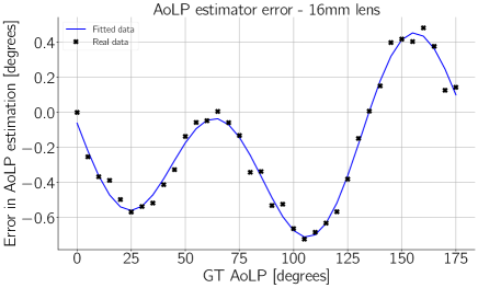
Figure 9: Error in the AoLP and curve fitted of Eq. 30 for the lens 3

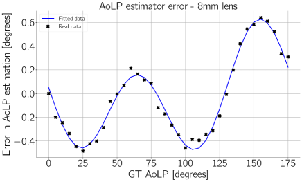
Figure 10: Error in the AoLP and curve fitted of Eq. 30 for the lens 1

By using a least-squares optimizer, the pixel parameters have been found for each set of samples taken with these lenses, and the results are shown in Tab. III. For creating this data, the degree of linear polarization was supposed to be $\rho=0.97$.

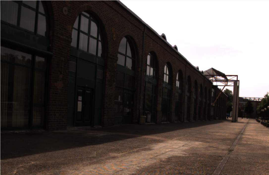
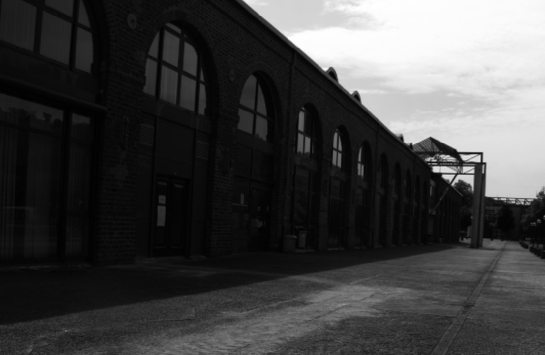
(a)	(b)
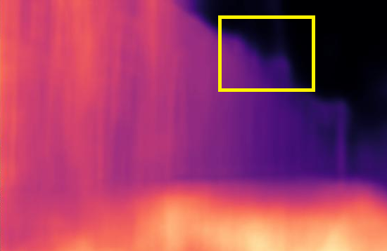
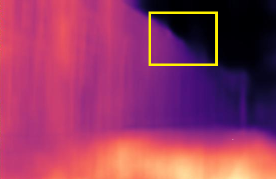
(c)	(d)

Figure 11: Monocular disparity application example (hotter colors indicate larger disparity, i.e., smaller depth values). (a) Original color image. (b) Total intensity image (c) Disparity computed with the uncalibrated intensities. (d) Disparities computed with the calibrated intensities.

Lens model	Parameter	$i=\left\{0,45,90,135\right\}$
$T_{i}$	Lens 1	$\left[0.53,0.48,0.49,0.51\right]$
	Lens 2	$\left[0.525,0.542,0.548,0.499\right]$
$P_{i}$	Lens 1	$\left[1.04,0.88,0.97,0.95\right]$
	Lens 2	$\left[1.009,0.992,1.067,0.922\right]$
$\varDelta\theta_{i}$	Lens 1	$\left[1.47,-1.07,-1.32,1.54\right]$
	Lens 2	$\left[0.109,0.114,-0.192,0.092\right]$

TABLE III: Parameters obtained by non-linear optimization for Eq. 30.

As shown in Figs. 10 and 9, taking the measurements of the AoLP from the center pixels and doing their circular average, produces an estimation of the true AoLP with a maximum error of $0.65^{\circ}$. This upper limit is valid for both lenses.

Tab. III shows all the pixel parameters obtained by least-squares optimization of Eq. 30 with the real data. From this table it is possible to confirm that the effective pixel values are not far away from the ideal ones. Particularly, the maximum orientation error is $\varDelta\theta_{0}=1.47^{\circ}$. Nonetheless, as explained in the previous section, this error is compensated by the complementary pixel orientation which is, in this case, $\varDelta\theta_{90}=-1.32^{\circ}$. Additionally, the values exposed in this table show that the two lenses influence the pixel parameters. Indeed, the figures have similar shapes, but the corresponding maximum values are not the same, and they are located at different positions. This is because the corresponding pixel parameters have changed for each case. It is important to highlight that the estimation error in the AoLP is limited, and small (less than $0.65^{\circ}$), confirming that the initial assumption of taking central pixels produces good estimates.

Appendix B: Applications tested with and without calibration

Since it is important to show the benefits of calibrating the RGB polarization camera in practical robot perception tasks, we have selected two testing algorithms for 3D geometry estimation. One for indoor and more suitable for small scale objects (shape-from-polarization), and one data-driven depth estimation approach from polarization images adapted to outdoor scenes. These algorithms are:

• “Linear depth estimation from an uncalibrated, monocular polarisation image”, ECCV, 2016 [30]: This paper proposes a shape-from-polarization algorithm with a linearization method for depth estimation, without any knowledge of the position of the light source. It is a geometric model-based approach, i.e., it does not use machine learning training phase for arriving to the results. We used the publicly available implementation in MatLab from the authors.

• “P2D: a self-supervised method for depth estimation from polarimetry”, ICPR 2020 [3]: This paper proposes a deep learning method for monocular disparity estimation, using monochrome polarization images. This network has been implemented considering the features given by the polarization state of the light. The code (in Python and PyTorch) and pre-trained model weights have been kindly provided by the authors of the paper upon our request.

The first experiment was the 3D reconstruction of a metallic, polished, parabolic object. This object has been placed at the interior of a dome, that provides a uniform, unpolarized, red light. The image has been captured with the camera that contains the Sony Polarsens sensor IMX250MYR, and a lens Fujinon HF8XA-5M. The object has been captured 1000 times, and the images have been averaged to reduce the influence of the noise. The camera has been calibrated, and then the intensities in the average image have been corrected with it. The reconstructed surfaces with and without calibration are shown in Fig. 12.

(a)	(b)
(c)	(d)

Figure 12: 3D reconstruction application result. (a) Original piece - front view. (b) Original piece - top view. (c) 3D reconstruction top view of the piece with the uncalibrated camera. (d) 3D reconstruction top view of the piece with the calibrated camera.

The areas of interest in this figure are highlighted with a green rectangle in the corresponding images. The corresponding images with the camera uncalibrated and calibrated are shown in the columns (c) and (d). In the reconstruction plots, we can notice two discontinuities. Since the surface is the result of an integration, the error in the normal’s estimation will produce that the closing points, i.e., the region where the end joins the beginning of the surface, will not match. The error in the normal vectors is linked to the error in the estimation of AoLP and the DoLP (due to the pixel’s parameters dispersion). These reconstruction artifacts have been reduced after calibration, with only one discontinuity in the surface with a reduced amplitude. It is important to mention that the same input images have been used for the two reconstructed surfaces. The uncalibrated reconstruction is done by using the raw image from the camera (after average), and the calibrated surface is obtained after correcting the measurements of the raw image. The second application corresponds to a monocular disparity estimation technique using a deep neural network. The results before and after calibration are shown in Fig. 11. Again, some areas of interest are highlighted in yellow. Since the network was trained with monochrome polarization images, the total intensity per polarization channel have been computed and given to the network to produce the estimation.

In this case, we can notice that after calibration the roof region is improved. In the uncalibrated scenario, the network predicts a disparity that ascends towards the sky, and when the image is calibrated, the disparity of this region evolves following the border of the roof. There are two considerations that might explain this behavior: i) The sky is polarized, so the features given by it are very distinctive from the building. ii) Neural networks base their predictions per pixel considering its value and the ones of the neighbors pixels. An uncalibrated setup will estimate wrong polarization parameters due to the dispersion in the pixel parameters and due to the lens. Particularly, as explained in the paper, the lens will produce a change in the polarization state depending on the point of incidence of the light at the lens surface. This change will create a gradient in the values different to the one present in the real scene. By doing the calibration, we reduce the lens effect, and therefore making the depth estimation between objects closer to the one in the real-scene.

References

- [1] Yunhao Ba, Alex Gilbert, Franklin Wang, Jinfa Yang, Rui Chen, Yiqin Wang, Lei Yan, Boxin Shi, and Achuta Kadambi. Deep shape from polarization. In European Conference on Computer Vision, 2020.
- [2] Kai Berger, Randolph Voorhies, and Larry H. Matthies. Depth from stereo polarization in specular scenes for urban robotics. In IEEE International Conference on Robotics and Automation (ICRA), 2017.
- [3] Marc Blanchon, Désiré Sidibé, Olivier Morel, Ralph Seulin, Daniel Braun, and Fabrice Meriaudeau. P2D: a self-supervised method for depth estimation from polarimetry. In International Conference on Pattern Recognition (ICPR), 2020.
- [4] Zhenyue Chen. Calibration method of microgrid polarimeters with image interpolation. Applied Optics, 54:995–1001, 02 2015.
- [5] Yingkai Cheng, Zhongmin Zhu, Zuodong Liang, Leanne Iannucci, Spencer Lake, and Viktor Gruev. Analysis of signal-to-noise ratio of angle of polarization and degree of polarization. OSA Continuum, 4, 04 2021.
- [6] Zhaopeng Cui, Viktor Larsson, and Marc Pollefeys. Polarimetric relative pose estimation. In IEEE/CVF International Conference on Computer Vision (ICCV), 2019.
- [7] Zhichao Ding, Chunsheng Sun, Hongwei Han, Liheng Ma, and Yonggang Zhao. Calibration method for division-of-focal-plane polarimeters using nonuniform light. IEEE Photonics Journal, 12 2020.
- [8] Huang Fei, Fan-Ming Li, Wei-Cong Chen, Rui Zhang, and Chao-Shuai Chen. Calibration method for division of focal plane polarimeters. Applied Optics, 57:4992, 06 2018.
- [9] Daoyi Gao, Yitong Li, Patrick Ruhkamp, Iuliia Skobleva, Magdalena Wysocki, HyunJun Jung, Pengyuan Wang, Arturo Guridi, and Benjamin Busam. Polarimetric pose prediction. In European Conference on Computer Vision (ECCV), October 2022.
- [10] Missael García, Ignacio Erausquin, Christopher Edmiston, and Viktor Gruev. Surface normal reconstruction using circularly polarized light. Optics Express, 23:14391, 06 2015.
- [11] Yilbert Gimenez, Pierre-Jean Lapray, Alban Foulonneau, and Laurent Bigué. Calibration algorithms for polarization filter array camera: survey and evaluation. Journal of Electronic Imaging, 29:1, 03 2020.
- [12] Nathan Hagen, Shuhei Shibata, and Yukitoshi Otani. Calibration and performance assessment of microgrid polarization cameras. Optical Engineering, 58:1, 02 2019.
- [13] E. Hecht. Optics. Pearson education. Addison-Wesley, 2002.
- [14] Tomoki Ichikawa, Matthew Purri, Ryo Kawahara, Shohei Nobuhara, Kristin Dana, and Ko Nishino. Shape from sky: Polarimetric normal recovery under the sky. In IEEE/CVF Conference on Computer Vision and Pattern Recognition (CVPR), 2021.
- [15] Francisco Iglesias and Alex Feller. Instrumentation for solar spectropolarimetry: State of the art and prospects. Optical Engineering, 58:1, 04 2019.
- [16] Lucid Vision Labs. Beyond conventional imaging: Sony’s polarized sensor, 2022-01-30.
- [17] Connor Lane, David Rode, and Thomas Roesgen. Calibration of a polarization image sensor andinvestigation of influencing factors. Applied Optics, 61, 10 2021.
- [18] P. Marconnet, Luc Gendre, A. Foulonneau, and Laurent Bigué. Cancellation of motion artifacts caused by a division-of-time polarimeter. Proc SPIE, 8160, 09 2011.
- [19] Olivier Morel, Ralph Seulin, and David Fofi. Handy method to calibrate division-of-amplitude polarimeters for the first three stokes parameters. Optics Express, 24:13634, 06 2016.
- [20] Olivier Morel, Christophe Stolz, Fabrice Meriaudeau, and Patrick Gorria. Active lighting applied to three-dimensional reconstruction of specular metallic surfaces by polarization imaging. Applied optics, 45:4062–8, 07 2006.
- [21] Tingkui Mu, Chunmin Zhang, Qiwei Li, and Rongguang Liang. Error analysis of single-snapshot full-stokes division-of-aperture imaging polarimeters. Optics Express, 23:10822–10835, 04 2015.
- [22] Samuel Powell, Roman Garnett, Justin Marshall, Charbel Rizk, and Viktor Gruev. Bioinspired polarization vision enables underwater geolocalization. Science Advances, 4, 04 2018.
- [23] S Powell and Viktor Gruev. Calibration methods for division-of-focal-plane polarimeters. Optics express, 21:21039–21055, 09 2013.
- [24] Joaquin Rodriguez, Lew Lew-Yan-Voon, Renato Martins, and Olivier Morel. A practical calibration method for rgb micro-grid polarimetric cameras: Paper supplemental material repository. https://github.com/vibot-lab/PoliCalibration, 2022.
- [25] E. Salomatina-Motts, V. Neel, and Anna Yaroslavsky. Multimodal polarization system for imaging skin cancer. Optics and Spectroscopy, 107:884–890, 12 2009.
- [26] Yoav Y. Schechner. Self-calibrating imaging polarimetry. In IEEE International Conference on Computational Photography, 2015.
- [27] Robert W. Schmieder. Stokes-algebra formalism. J. Opt. Soc. Am., 59(3):297–302, Mar 1969.
- [28] Moein Shakeri, Shing Yan Loo, and Hong Zhang. Polarimetric monocular dense mapping using relative deep depth prior, 2021.
- [29] S. Shwartz, E. Namer, and Y.Y. Schechner. Blind haze separation. In IEEE Computer Society Conference on Computer Vision and Pattern Recognition (CVPR), 2006.
- [30] William A. P. Smith, Ravi Ramamoorthi, and Silvia Tozza. Linear depth estimation from an uncalibrated, monocular polarisation image. In Bastian Leibe, Jiri Matas, Nicu Sebe, and Max Welling, editors, European Conference on Computer Vision (ECCV), 2016.
- [31] Frans Snik, Julia Craven-Jones, Michael Escuti, Silvano Fineschi, David Harrington, Antonello De Martino, Dimitri Mawet, Jérôme Riedi, and J. Scott Tyo. An overview of polarimetric sensing techniques and technology with applications to different research fields. In David B. Chenault and Dennis H. Goldstein, editors, Polarization: Measurement, Analysis, and Remote Sensing XI, volume 9099, pages 48 – 67. International Society for Optics and Photonics, SPIE, 2014.
- [32] Shoji Tominaga and Akira Kimachi. Polarization imaging for material classification. Optical Engineering - OPT ENG, 47, 12 2008.
- [33] Xingzhou Tu, Oliver J. Spires, Xiaobo Tian, Neal Brock, Rongguang Liang, and Stanley Pau. Division of amplitude rgb full-stokes camera using micro-polarizer arrays. Opt. Express, 25(26), 2017.
- [34] J. Tyo. Optimum linear combination strategy for an n -channel polarization- sensitive imaging or vision system. Journal of The Optical Society of America, 15, 02 1998.
- [35] Yannick Verdié, Jifei Song, Barnabé Mas, Benjamin Busam, Ales Leonardis, and Steven McDonagh. Cromo: Cross-modal learning for monocular depth estimation. In Proceedings of the IEEE/CVF Conference on Computer Vision and Pattern Recognition (CVPR), pages 3937–3947, June 2022.
- [36] Zhixiang Wang, Yinqiang Zheng, and Yung-Yu Chuang. Polarimetric camera calibration using an lcd monitor. In IEEE/CVF Conference on Computer Vision and Pattern Recognition (CVPR), 2019.
- [37] Xuesong Wu, Hong Zhang, Xiaoping Hu, Moein Shakeri, Chen Fan, and Juiwen Ting. Hdr reconstruction based on the polarization camera. IEEE Robotics and Automation Letters, 5(4):5113–5119, 2020.
- [38] Lei Yan, Taixia Wu, and Xueqi Wang. Polarization remote sensing for land observation, 2018.
- [39] Luwei Yang, Feitong Tan, Ao Li, Zhaopeng Cui, Yasutaka Furukawa, and Ping Tan. Polarimetric dense monocular slam. In IEEE/CVF Conference on Computer Vision and Pattern Recognition, 2018.