Prompt Tuning with Soft Context Sharing for Vision-Language Models

Abstract

Vision-language models have recently shown great potential on many computer vision tasks. Meanwhile, prior work demonstrates prompt tuning designed for vision-language models could acquire superior performance on few-shot image recognition compared to linear probe, a strong baseline. In real-world applications, many few-shot tasks are correlated, particularly in a specialized area. However, such information is ignored by previous work. Inspired by the fact that modeling task relationships by multi-task learning can usually boost performance, we propose a novel method SoftCPT (Soft Context Sharing for Prompt Tuning) to fine-tune pre-trained vision-language models on multiple target few-shot tasks, simultaneously. Specifically, we design a task-shared meta network to generate prompt vector for each task using pre-defined task name together with a learnable meta prompt as input. As such, the prompt vectors of all tasks will be shared in a soft manner. The parameters of this shared meta network as well as the meta prompt vector are tuned on the joint training set of all target tasks. Extensive experiments on three multi-task few-shot datasets show that SoftCPT outperforms the representative single-task prompt tuning method CoOp [78] by a large margin, implying the effectiveness of multi-task learning in vision-language prompt tuning. The source code and data will be made publicly available.

1 Introduction

Vision-language models [60, 32, 50] especially the contrastive learning based ones (CLIP [60], SLIP [55]) pre-trained on large-scale image-text pairs collected from the web have recently obtained extensive attention due to their potential applications to open-vocabulary tasks [19, 21, 25], which are known as important and challenging problems in computer vision. Besides the openness of natural language supervision against fixed discrete label supervision, the abundant semantic information implied in the learned visual features as well as the versatility of the text encoder as a language prior also contributes to the success of contrastive vision-language models. Increasing evidences indicate that improved performance can be achieved by transferring knowledge from vision-language models to computer vision tasks, such as zero-shot classification [60, 78], few-shot classification [60, 78, 14], object detection [19, 21, 25], image segmentation [62, 52], image captioning [54], and text-to-image generation [64, 41].

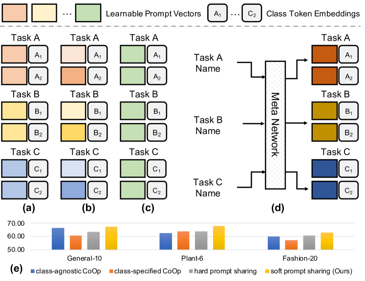
Figure 1: A conceptual comparison of different prompt tuning methods. (a) class-agnostic CoOp, (b) class-specified CoOp, (c) hard prompt sharing for CoOp, (d) our soft prompt sharing, (e) average performances on three datasets. In (a)-(d), we assume there are 2 classes per task and shared prompt vectors are colored in the same color. The proposed SoftCPT uses softly-shared prompt vectors, which obtains better performance as shown in (e).

Provided with pre-trained vision-language models, how to adapt their implicit knowledge to various downstream tasks becomes an essential problem to care about. Inspired by the fine-tuning techniques in natural language processing (NLP) [65, 34], Zhou et al. [78] recently proposed CoOp that introduces prompt tuning, first raised in NLP [48, 47, 42], to computer vision for addressing the problem of few-shot image recognition. In particular, a learnable prompt vector (also called context with CoOp’s terminology) is concatenated with the token embeddings of class name, and they are fed to the text encoder to generate classifier weight, subsequently. Both the parameters of image and text encoder are frozen during training. Meanwhile, for a certain few-shot task, all classes can share a unified prompt vector in a class-agnostic way or each class can learn its own prompt vector in a class-specified way. As reported by their work, CoOp can achieve improved accuracy against a strong baseline – linear probe [72]. CoOp paves a new way to solve the visual few-shot recognition problem. Following this path, CoCoOp [77] addresses the class shift problem of CoOp by making the prompt vector be dependent on input image. DualCoOp [70] adapts pre-trained vision-language models to multi-label recognition task with limited annotations. ProDA [51] learns a collection of diverse prompts and adopts multivariate Gaussian distribution to model these prompts. Improved performances are observed by using prompt ensembling.

The “pre-train then prompt-tune” paradigm suggests in future at least for some specialized areas there is only need to keep one copy of the “universal” pre-trained model and activate it to accommodate to various downstream tasks. In real-life applications, it is very natural to assume there are some relationships between these tasks. For example, in the online E-commerce scenario, predicting the top type and collar type of clothes are two highly related tasks. In fact, it is very uncommon that padded jacket has a tailored collar. From prior work, jointly training a model on some related tasks in a multi-task manner is believed to be helpful for improving performance [13, 36]. Therefore, we naturally pose a question: whether prompt tuning of vision-language models can benefit from multi-task learning? Although multi-task learning has already been introduced to prompt tuning for pure language models [7, 58, 59, 69], the multi-task prompt tuning for vision-language domain is still absent. This reveals the necessity of answering this question.

To research the effectiveness of multi-task prompt tuning, our initial attempt is adapting CoOp by sharing a class-agnostic prompt vector across all target tasks and tuning this prompt vector on joint multi-task few-shot training set. However, the performance of this hard prompt sharing (see Fig. 1(e)) is unstable, it underperforms on General-10 dataset, probably due to the loose relations between the tasks on this generalized dataset. To tackle this problem, we relax the hard constraint by sharing the prompt vectors in a soft manner and propose a new multi-task prompt tuning technique called SoftCPT (Soft Context Sharing for Prompt Tuning), as depicted by Fig. 1(d). To be more specific, a shared meta network is devised to generate per-task soft (i.e., continuous) prompt. The meta network takes as inputs a learnable meta prompt vector and pre-defined task name, and the concatenation of them is fed to CLIP’s text encoder to generate task feature (ref. Fig. 2(b)). The task feature is then processed by a simple sub-network to generate the soft prompt vector. Both the meta prompt vector and the parameters of the meta network are jointly trained in a multi-task manner. Due to the capability of extracting semantic feature of CLIP’s text encoder, similar task names would result in similar soft prompt vectors instead of identical ones. Besides, the meta prompt also plays a role of modulating the similarity between soft prompts.

We conduct several experiments on three multi-task few-shot datasets: a generalized dataset General-10 built from 10 public image classification datasets, a specialized dataset Plant-6 for plant classification that is consisted of 6 tasks, and a specialized dataset Fashion-20 that is collected by us and has 20 tasks about fashion classification. Our results show the proposed SoftCPT outperforms CoOp by 0.73%, 5.09% and 2.80% on these datasets, respectively, which hints multi-task prompts are beneficial to downstream tasks. Our contributions are summarized as follows:

1. A softly-shared multi-task prompt tuning method SoftCPT is proposed for vision-language models, which consists of a novel meta network that transforms task name to prompt vector. To our knowledge, this is the first work to explore the effectiveness of multi-task learning in prompt tuning for vision-language models.

2. A new few-shot fashion classification dataset is constructed to test the effectiveness of multi-task prompt tuning in real industrial scenario, which will be made publicly available soon to facilitate future researches.

3. Experiments on three datasets, ranging from generalized to specialized area, are conducted to study the efficacy of SoftCPT. Our results demonstrate multi-task prompts if learned in a soft sharing manner are indeed useful for the scenarios with multiple related tasks.

2 Related Work

2.1 Pre-trained Models

The paradigm of pre-training deep neural networks on large-scale datasets and then applying the models to annotation-scarce domains by fine-tuning has become mainstream in language, vision and vision-language domain. In the language domain, with the occurrence of Transformers [73], deeper language models with increasing number of parameters are put forward. The 12-layer BERT [15] proposed in 2018 has 110M parameters, while the Switch Transformer [20] proposed in 2021 has 1.6T parameters, a 15000x increase in model size. Large-scale language models have shown great benefits for improving performance in past few years, making them become the focus of AI research [27]. In the vision domain, motivated by the success of Transformers, a paradigm shift from CNNs (ResNets [28]) to Transformers (ViT [18], Swin Transformer [49]) has emerged. In the vision-language domain, learning multi-modal models from web-scale data with natural language supervision [60, 32, 50] has achieved significant progress on zero-shot and few-shot learning. In summary, pre-training plays a key role in current AI research.

2.2 Vision-Language Models

We further review related pre-training models in the vision-language domain in detail. Existing methods of modeling vision and language signals can be roughly categorized as one-stream and two-stream methods. The former processes inputs from different modalities into a unified token sequence and models their relationship with BERT. Related work includes VisualBERT [46], Unicoder-VL [45] and ViLT [38]. The frequently-used objectives in this case are MLM loss [15], masked region modeling loss [11] and matching loss [11, 66, 50]. The latter uses an image encoder (e.g., ResNets, ViT) and a text encoder (e.g., BERT) to encode the visual and text inputs separately. The image and text features are usually related in a unified embedding space by contrastive loss [60, 75, 55, 32, 50]. The strength of the contrastive based two-stream method is that a good visual feature extractor can be learned. In CLIP [60], strong zero-shot performance is achieved, which demonstrates the extracted visual features are of superior generalization ability. Moreover, the text encoder can also be regarded as a language prior that is proved to be quite useful in many vision tasks [78, 14, 62, 52]. Finally, the openness of the vocabulary in vision-language models makes them be suitable for open-vocabulary tasks [19, 21, 25], either.

2.3 Parameter-Efficient Fine-Tuning

With the rapid development of pre-training techniques, lots of pre-trained models are available as mentioned above. The constant increase of model size poses a new challenge – how to fine-tune the models in a parameter-efficient way on new tasks. Traditional fine-tuning method [15, 31, 16, 76] adds task-specific heads and tunes all parameters. Although it is simple and extensively adopted, it has several obvious deficiencies. [33] stated that fine-tuning is prone to overfit on small datasets.  [40] found fine-tuning can distort pre-trained features and underperform out-of-distribution. In addition, when facing many target tasks, fine-tuning separately for each task is storage inefficient in both training and testing stage [7]. In view of this, two kinds of parameter-efficient fine-tuning methods are proposed, i.e., prompt-based [61, 9, 65, 24, 48, 47, 78, 51] and adapter-based [30, 63, 35, 23, 71] methods. The prompt-based methods freeze all parameters and only design or optimize the inputs of models on different tasks. In essence, they try to map target distribution to source distribution by modifying the inputs. Prompt-based methods can be further categorized into prompt design [61, 9], prompt search [65, 24] and prompt tuning [48, 47, 78, 51]. Compared to prompt design and prompt search, prompt tuning is more favorable as it avoids time-consuming handcrafting [65] and the introduction of extra complexities [24]. As for adapter-based methods, they freeze the model parameters and insert or attach some tuneable layers, whose parameters will be tuned on target task. With recent development, prompt-based and adapter-based methods can now achieve comparable or even better performance compared to fine-tuning in both language [26] and vision [35, 78, 51] domain.

2.4 Prompt Tuning for Vision-Language Models

Inspired by the success of prompt tuning in NLP, Zhou et al. [78] proposed a method CoOp that first introduces prompt tuning to vision-language models. The difference compared to the practice in language domain lies in the MASK token in CoOp is replaced with different text labels to better fit the constrastive loss in CLIP. Following this line, several prompt tuning methods are proposed to further improve the effectiveness and versatility for few-shot recognition task, such as CoCoOp [77], DualCoOp [70], and ProDA [51]. The idea of prompt tuning is also applied to other vision tasks, e.g., image segmentation [62].

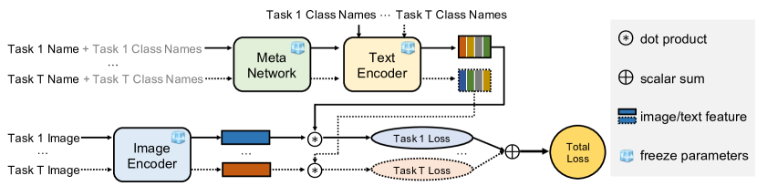
(a) The overall network structure of SoftCPT.

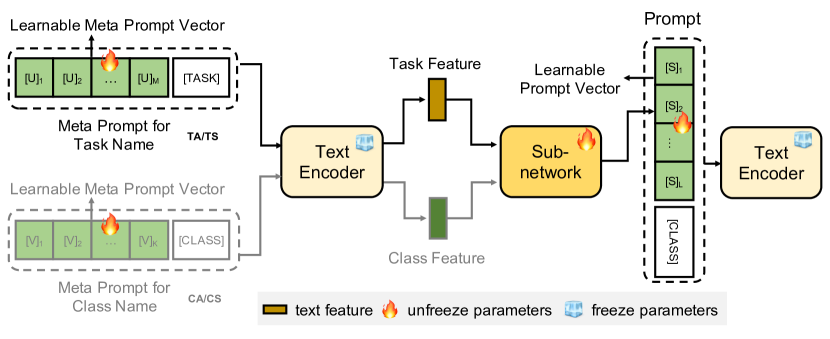
(b) Structure of the meta network.

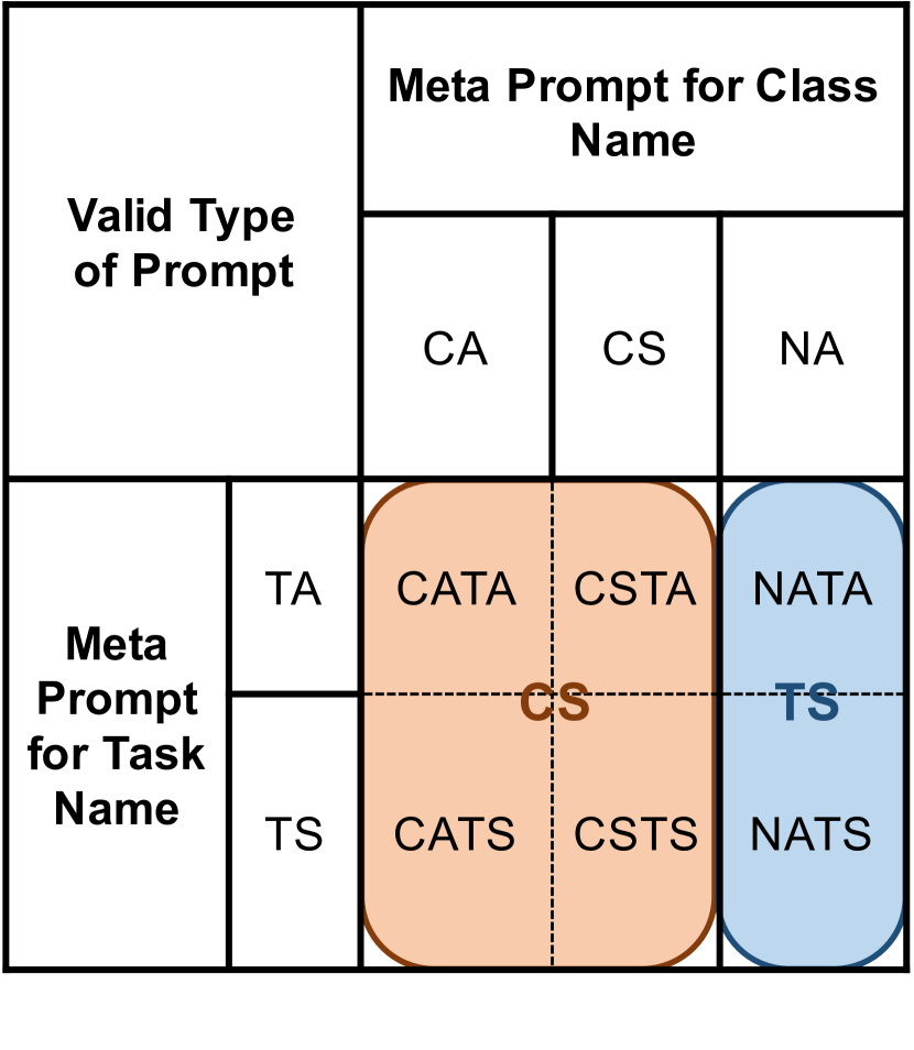
(c) Valid type of prompt.

Figure 2: Illustration of the proposed multi-task prompt tuning method SoftCPT. SoftCPT uses samples of all tasks for training and the loss is computed independently for each task. The summed loss is calculated for backpropagation. The meta network could generate task-specific or class-specific prompt vectors. However, we find task-specific way could acquire desirable performance with higher computational efficiency. In (b), [TASK] denotes token embeddings of task name. [CLASS] denotes token embeddings of a certain class name in a task. CA: class-agnostic, CS: class-specified, TA: task-agnostic, TS: task-specified, NA: no meta prompt for class name.

2.5 Multi-Task Learning

Multi-task learning (MTL) is an important subfield in machine learning [10, 13]. By exploiting task relatedness, it is able to improve the performance over single-task learning. The underlying principles lie in improved data efficiency and reduced overfitting by sharing representations. There are two dominant methods for deep multi-task learning, hard and soft parameter sharing, which learn identical and similar features, respectively. Recently, MTL has been introduced to prompt tuning in NLP. For instance, [7] adopted MTL to learn the parameters of attention generator and slightly improved performances are observed on language tasks.  [59] proposed to learn a universal intrinsic task subspace in a multi-task manner. The back-projected prompt vectors do not reduce the task performance a lot, which implies the learned prompt vectors of different NLP tasks have a low-dimensional structure. By comparison, the MTL for prompt tuning is conducted on inputs, which is different from the traditional MTL that is performed on features. Therefore, the research of MTL for prompt tuning is necessary. Finally, although MTL is proved promising in NLP, its efficacy on prompt tuning for vision-language models has not been studied yet. Our work fills this gap.

2.6 Few-Shot Learning

Human being has the ability to recognize new categories with limited samples. Few-shot learning [43] aims at studying how to endow machines with such an ability. Typical methods include modeling the similarities between query and supports [67, 17] and learning a good initialization for fast adaption [22]. Recently, CoOp [78] solves the few-shot learning problem with prompt tuning, which belongs to the category of directly generating model weights adapted to new task with support set. Our work follows this line and studies whether MTL is beneficial for prompt tuning of vision-language models.

3 Method

3.1 Overview

The overall structure of SoftCPT is given in Fig. 2(a). It inherits the two-stream structure from CLIP to bridge the gap between pre-training and fine-tuning. In this figure, the bottom part represents the image branch that encodes input image into visual feature, while the top part represents the text branch that generates classifier weights by transforming the class name and task name.

Assume there are $T$ tasks, let $\boldsymbol{x}_{t}$ be an example sampling from the $t$-th task. The image encoder $e(\cdot)$ extracts the visual feature of $\boldsymbol{x}_{t}$, which is denoted as $e(\boldsymbol{x}_{t})$. For the $t$-th task, a group of classifier weights are generated by text encoder (the method will be discussed later), that are $[\boldsymbol{w}_{t,1},\cdots,\boldsymbol{w}_{t,c},\cdots,\boldsymbol{w}_{t,{C_{t}}}]$, where $C_{t}$ denotes the class number of the $t$-th task and $\boldsymbol{w}_{t,c}$ is the classifier weight of class $c$ in task $t$. The prediction probability of $\boldsymbol{x}_{t}$ belonging to the $c$-th class is

$$p(y=c|\boldsymbol{x}_{t})=\frac{\exp(\langle e(\boldsymbol{x}_{t}),\boldsymbol{w}_{t,c}\rangle/\tau)}{\sum\nolimits_{i=1}^{C_{t}}\exp(\langle e(\boldsymbol{x}_{t}),\boldsymbol{w}_{t,i}\rangle/\tau)}$$ (1)

where $\langle\cdot,\cdot\rangle$ denotes the dot product between two vectors and $\tau$ is a temperature parameter [60].

For fast model adaption, the language prior implied in the text encoder of CLIP is adopted. To avoid destroying such a prior, prompt tuning is resorted to activate the text encoder to generate good classifier on target tasks. Different from prior work, we attempt to exploit the relations between target tasks to learn better prompts. For this aim, a meta network is devised to generate task-specified or class-specified prompt vectors. These prompt vectors as well as class names will be fed to text encoder to obtain the final classifier weights for all tasks.

Fig. 2(b) illustrates the structure of the meta network. For the task-specified way, the text encoder first transforms the meta prompt for task, which is consisted of a learnable meta prompt vector and a task name, into task feature. A sub-network is then resorted to transform the task feature into prompt vector, which is sequentially combined with class name of this task to form a prompt. The prompt is finally sent to the text encoder to get the corresponding classifier weight. In this case, each task only learns one prompt vector. As for the class-specified way, class feature generated by text encoder is viewed as an extra input to the sub-network. For a task, $C$ prompt vectors will be generated by the sub-network if there are $C$ classes in this task. The meta prompt for task could be task-agnostic or task-specific, while the meta prompt for class, if any, cloud be class-agnostic or class-specific. The valid six combinations of them are shown in Fig. 2(c).

3.2 Task-Specified Prompts

We only present the task-agnostic meta prompt for task name in this case and the extension to the task-specific case is trivially implemented by learning one independent meta prompt vector for each task name. For task-agnostic meta prompt, only one shared meta prompt for descriptive text of all tasks is required, which is designed to have the form $\boldsymbol{u}=[\text{U}]_{1}[\text{U}]_{2}\cdots[\text{U}]_{M}[\text{TASK}]$ with $[\text{U}]_{1}[\text{U}]_{2}\cdots[\text{U}]_{M}$ the learnable meta prompt vector and $[\text{TASK}]$ the token embedding sequence of a certain task name. $[\text{U}]_{m}$ ($m\in\{1,\cdots,M\}$) is a vector with the same dimension as word embeddings in CLIP and $M$ is the length of the meta prompt vector.

The text encoder $g(\cdot)$ of CLIP accepts as input the meta prompt $\boldsymbol{u}$ and extracts the task feature $g(\boldsymbol{u})$. To get the prompt vector, a sub-network $s(\cdot)$ is designed, whose structure will be detailed later. By forwarding $g(\boldsymbol{u})$ to $s(\cdot)$, the prompt vector for a task is obtained, i.e., $[\text{S}]_{1}[\text{S}]_{2}\cdots[\text{S}]_{L}=s(g(\boldsymbol{u}))$, where $L$ is the prompt length and $[\text{S}]_{l}$ ($l\in\{1,\cdots,L\}$) is a vector with the same dimension as word embeddings in CLIP. By combing this prompt vector with class token embeddings $[\text{CLASS}]$, we obtain the prompt $\boldsymbol{s}=[\text{S}]_{1}[\text{S}]_{2}\cdots[\text{S}]_{L}[\text{CLASS}]$. Note that, $[\text{S}]_{1}[\text{S}]_{2}\cdots[\text{S}]_{L}$ is shared within a task, but not among tasks.

Finally, the text encoder transforms $\boldsymbol{s}$ into classifier weight vector, $\boldsymbol{w}=g(\boldsymbol{s})$. For task $t$, by replacing $[\text{TASK}]$ with the task name and $[\text{CLASS}]$ with each class name of this task, we obtain the classifier weights of the $c$-th class, i.e., $\boldsymbol{w}_{t,c}=g(\boldsymbol{s}_{t,c})$, $c\in\{1,\cdots,C_{t}\}$.

3.3 Class-Specified Prompts

We detail how to make class-specific prompts when meta prompt for task name is task-agnostic and meta prompt for class name is class-agnostic, while the extension to other cases is trivial. In this case, besides the task-agnostic meta prompt vector for task name, a meta prompt vector for all classes of all tasks is learned additionally. Similar to $\boldsymbol{u}$, the meta prompt for class name is defined as $\boldsymbol{v}=[\text{V}]_{1}[\text{V}]_{2}\cdots[\text{V}]_{K}[\text{CLASS}]$ with $K$ the prompt length and $[\text{V}]_{k}$ ($k\in\{1,\cdots,K\}$) a vector with the same length to $[\text{U}]_{m}$. By feeding the meta prompt $\boldsymbol{v}$ to the text encoder, we get the class feature $g(\boldsymbol{v})$. Different from the task-specified case, $g(\boldsymbol{v})$ and $g(\boldsymbol{u})$ are inputted to the sub-network $s(\cdot,\cdot)$ jointly. As a result, the prompt vector $[\text{S}]_{1}[\text{S}]_{2}\cdots[\text{S}]_{L}=s(g(\boldsymbol{u}),g(\boldsymbol{v}))$ for each class of a task is obtained. The prompt format in this case is defined as before, while the prompt vectors are not shared between any two classes.

3.4 Sub-network Design

The design of sub-network $s(\cdot)$ or $s(\cdot,\cdot)$ should consider two problems: how to process the inputs and how to design a data-efficient structure. For the first point, only the class-specified case needs to be treated as there are two inputs. We have tried two methods: 1) concatenating task feature and class feature into a long vector; 2) computing the mean of these two vectors. For the second point, only linear and MLP networks are tried due to their simplicity. Other structures like Transformers are not utilized here because they are more likely to suffer from scarce data. One should note that, before emitting the results, reshaping is performed by the sub-network to get the prompt vector with proper size.

3.5 Optimization

Unlike CoOp, SoftCPT is trained on the joint training set of all target tasks. Assume there are $T$ tasks, each has its own data splits. We define the dataset of task $t$ as $\mathcal{D}_{t}=(\mathcal{D}_{t}^{\text{train}},\mathcal{D}_{t}^{\text{val}},\mathcal{D}_{t}^{\text{test}})$, where $\mathcal{D}_{t}^{\text{train}}$, $\mathcal{D}_{t}^{\text{val}}$ and $\mathcal{D}_{t}^{\text{test}}$ denote the train, validation and test split, respectively. Each of these splits is a set of tuples, that is $\mathcal{D}^{*}_{t}=\{(\boldsymbol{x}_{t,i},y_{t,i})\}_{i=1}^{N^{*}_{t}}$, where $*$ is “train”, “val” or “test”, $\boldsymbol{x}_{t,i}$ is an image from task $t$ with label $y_{t,i}$, $N^{*}_{t}$ is sample size and $i$ is the index. We further define the joint dataset $\mathcal{D}$ as $\mathcal{D}=(\mathcal{D}^{\text{train}},\mathcal{D}^{\text{val}},\mathcal{D}^{\text{test}})$, where $\mathcal{D}^{\text{train}}$, $\mathcal{D}^{\text{val}}$ and $\mathcal{D}^{\text{test}}$ denote the joint train, validation and test set, respectively. $\mathcal{D}^{*}$ is the union of the samples from all tasks with the same split, i.e., $\mathcal{D}^{*}=\bigcup\nolimits_{t=1}^{T}\mathcal{D}^{*}_{t}$. For model training, the following total loss is minimized,

$$\mathcal{L}=-\sum\nolimits_{t=1}^{T}\sum\nolimits_{i=1}^{N^{\text{train}}_{t}}\log(p(y=y_{t,i}|\boldsymbol{x}_{t,i})),$$ (2)

where $p(y=y_{t,i}|\boldsymbol{x}_{t,i})$ is given by Eq. 1. The parameters to be optimized include the meta prompt vectors and meta network’s parameters, while all other parameters are fixed.

4 Experiment

4.1 Datasets

For thorough comparison, three multi-task few-shot datasets are constructed, ranging from generalized to specialized domain. The key information is listed below, for more details please refer to appendix.

General-10 is a generalized dataset built by combing 10 publicly available classification datasets (Caltech101 [44], DTD [12], EuroSAT [29], FGVCAircraft [53], Food101 [8], Flowers102 [56], Oxford-Pets [57], StanfordCars [39], SUN397 [74], and UCF101 [68]), including both coarse-grained and fine-grained tasks. These datasets are also adopted in CLIP and CoOp.

Plant-6 is a specialized multi-task few-shot dataset, which is built based on 6 public plant related classification datasets: FruitVegetable [3], KaggleFlower [2], KaggleMushroom [4], KaggleVegetable [6], PlantSeedling [5], and PlantVillage [1].

Fashion-20 is a specialized dataset for fashion classification (a key technique for product data governance on E-commerce platform), which is collected by us and has about 24K images in 20 tasks. All the images are obtained by searching on web using pre-defined keywords. Before human labeling, simple data cleaning is performed, e.g., removing similar or too small images. The 20 tasks are pants type, pants length, waist type, collar type, sleeve type, sleeve length, top pattern, shoe material, shoe style, heel shape, heel thickness, heel height, upper height, toe cap style, hat style, socks length, socks type, skirt length, number of button rows, and underwear style classification.

In addition, all datasets are split according to the strategy used in CoOp.

4.2 Implementation Details

In all prompt tuning based methods, CLIP is used as the pre-trained vision-language model. Unless otherwise specified, ResNet-50 is used as the image encoder. In the ablation study, other image backbones are also compared.

In SoftCPT, the task names are pre-defined. For example, the task names of Caltech101 and PlantSeedling are “object classification” and “plant seedling classification”, respectively. For a complete list of the names, please refer to appendix. For a fair comparison, the length of the prompt vector $L$ is set to be 16, which is identical to the setting in CoOp. As for $M$ and $K$, they are set to be 4 as default. For the initialization of meta prompt vectors, we use the simplest random method because task-specified initialization is unnecessary as reported in a recent work [37]. Besides, linear sub-network and feature concatenation are adopted as default for task-specific and class-specific prompts. Finally, SGD with an initial learning rate of 0.002 and a cosine decay scheduler are used for model optimization. The batch size is set to be 32 and 50 epochs are trained on all datasets for all prompt tuning methods.

For model evaluation, the test set performances are reported. For few-shot classification, to reduce the variance, the scores over three trials with different seeds are averaged like CoOp. For General-10, the same evaluation metrics to CLIP are used. For all tasks of Plant-6 and Fashion-20, top-1 accuracy is adopted. Besides linear probe and zero-shot recognition, test set metrics of the last checkpoints are reported, thus no validation is involved.

4.3 Main Results

The main results of different methods on three datasets are listed in Tab. 1. Five different methods are compared to ours: 1) Linear probe CLIP is a strong baseline reported in CLIP [60]; 2) CoOp-CA denotes the class-agnostic CoOp applied to each task separately; 3) CoOp-CS denotes the class-specific CoOp applied to each task separately; 4) CoOp-MT denotes a shared prompt vector for all tasks and all classes is learned in CoOp in a multi-task manner; 5) Zero-shot CLIP is adopted in [60] and manually-designed text templates are used to generate classifier weights. As for our method, we name it as SoftCPT-suffix, where “suffix” is a name (its length is 4) listed in the table of Fig. 2(c). However, here we only compare the results of SoftCPT-NATA and SoftCPT-NATS as they could acquire desirable performance with lower computational cost. The comparison of other combinations will be given in Sec. 4.4. From the table, it can be observed that SoftCPT-NATA improves the scores by 0.73%, 5.09%, 2.80% on General-10, Plant-6 and Fashion-20, respectively, compared to CoOp-CA. This demonstrates the effectiveness of the proposed method.

The results with increasing number of training samples are shown in Fig. 3(a)-(c). We can observe that SoftCPT achieves better scores than the other methods. What’s more, its performances are quite stable on both generalized and specialized dataset. However, the other methods, e.g., CoOp-CA, could acquire good results on one dataset but bad results on other datasets. It can be seen that the simple hard sharing of prompt vectors (CoOp-MT) is exceeded by the proposed soft sharing (SoftCPT) in most cases. One possible reason is that hard sharing is too restrict to scale with the increasing complexity of more tasks. Meanwhile, it is prone to introduce the so-called negative transfer [13] for tasks have weak relation to others. As for linear probe, it achieves good results on two specialized datasets, showing its strong ability of transfer learning.

Method	General-10	Plant-6	Fashion-20
LP-CLIP	56.96 $\pm$ 0.41	64.55 $\pm$ 0.73	60.11 $\pm$ 1.01
CoOp-CA	66.39 $\pm$ 0.52	62.59 $\pm$ 2.33	59.95 $\pm$ 1.11
CoOp-CS	60.70 $\pm$ 0.23	63.98 $\pm$ 0.94	57.16 $\pm$ 1.01
CoOp-MT	63.43 $\pm$ 0.46	63.90 $\pm$ 0.77	60.55 $\pm$ 1.37
ZS-CLIP	58.29 $\pm$ 0.00	50.96 $\pm$ 0.00	45.49 $\pm$ 0.00
SoftCPT-NATA	67.12 $\pm$ 0.39	67.68 $\pm$ 1.18	62.75 $\pm$ 0.60
SoftCPT-NATS	67.04 $\pm$ 0.23	67.13 $\pm$ 1.15	60.88 $\pm$ 1.08

Table 1: Overall numerical comparison of average score (%). LP-CLIP: Linear probe CLIP, ZS-CLIP: Zero-shot CLIP.

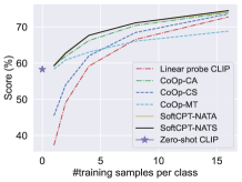
(a) Results on General-10

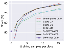
(b) Results on Plant-6

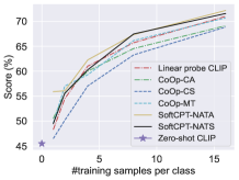
(c) Results on Fashion-20

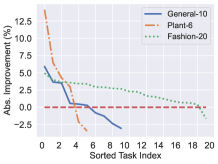
(d) Sorted Improvements

Figure 3: Performance with varying number of training samples (a)-(c) and per-task absolute improvements of SoftCPT-NATA over CoOp-CA sorted in descending order (d). In (a)-(c), the averaged score over all tasks is reported for each dataset. $M$ and $K$ are set to be 8 for better performance.

We further compare different methods from the task dimension. The per-task improvements of SoftCPT-NATA over CoOp-CA on all tasks are reported in Fig. 3(d). On most tasks multi-task training with soft prompt sharing achieves better performance. For specialized datasets, the per-task improvements are more significant.

4.4 Ablation Study

Effectiveness of Merging More Tasks. We merge General-10 and Plant-6 into a new dataset and conduct experiments to study if combing more tasks can bring extra benefits. The experimental results are listed in Tab. 2. By excluding the influence of using task names as extra inputs, multi-task learning does contribute to improve overall performance.

Learning Meta Prompt for Class Is Necessary? We conduct experiments of SoftCPT with different configurations as listed in Fig. 2(c). For class-specific prompts, more gradients should be stored, thus more GPU memory is required. For example, more than 40G GPU memory is required for SoftCPT-CSTA with FP16 training, which is not affordable on most GPU cards. To reduce memory, a portion of all class names are randomly sampled for loss computation. On General-10, the sampling rate is 10%, while on the other two datasets no sampling is used as there are not too many classes. The results are reported in Tab. 3. Clearly, task-specific prompt already achieves good performance on all datasets. Considering the high computational cost of the class-specific manner, it is thus not recommended.

$\mathcal{D}^{\text{train}}$	$\mathcal{D}^{\text{test}}$	Score (%)
$\mathcal{D}^{\text{train}}_{\text{G}}$	$\mathcal{D}^{\text{test}}_{\text{G}}$	67.16 $\pm$ 0.38
$\mathcal{D}^{\text{train}}_{\text{G}}\cup\mathcal{D}^{\text{train}}_{\text{P}}$	$\mathcal{D}^{\text{test}}_{\text{G}}$	67.15 $\pm$ 0.34
$\mathcal{D}^{\text{train}}_{\text{P}}$	$\mathcal{D}^{\text{test}}_{\text{P}}$	67.22 $\pm$ 1.11
$\mathcal{D}^{\text{train}}_{\text{G}}\cup\mathcal{D}^{\text{train}}_{\text{P}}$	$\mathcal{D}^{\text{test}}_{\text{P}}$	68.41 $\pm$ 0.95
$\mathcal{D}^{\text{train}}_{\text{G}}$ or $\mathcal{D}^{\text{train}}_{\text{P}}$	$\mathcal{D}^{\text{test}}_{\text{G}}\cup\mathcal{D}^{\text{test}}_{\text{P}}$	67.18 $\pm$ 0.33
$\mathcal{D}^{\text{train}}_{\text{G}}\cup\mathcal{D}^{\text{train}}_{\text{P}}$	$\mathcal{D}^{\text{test}}_{\text{G}}\cup\mathcal{D}^{\text{test}}_{\text{P}}$	67.62 $\pm$ 0.39

Table 2: Average results of SoftCPT-NATA with different combinations of train and test sets. $\mathcal{D}^{\text{train/test}}_{\text{G}}$ and $\mathcal{D}^{\text{train/test}}_{\text{P}}$ denote a split of General-10 and Plant-6, respectively. “$\mathcal{D}^{\text{train}}_{\text{G}}$ or $\mathcal{D}^{\text{train}}_{\text{P}}$” denotes two models are trained on General-10 and Plant-6 independently.

Prompt	Config	General-10	Plant-6	Fashion-20
class specific	CATA	63.71 $\pm$ 0.69	66.87 $\pm$ 1.33	58.51 $\pm$ 1.39
	CSTA	63.11 $\pm$ 0.63	67.60 $\pm$ 0.91	57.81 $\pm$ 1.66
	CATS	64.40 $\pm$ 0.57	67.04 $\pm$ 0.80	59.38 $\pm$ 1.18
	CSTS	62.70 $\pm$ 0.72	67.08 $\pm$ 1.77	57.55 $\pm$ 1.16
task specific	NATA	67.16 $\pm$ 0.38	67.22 $\pm$ 1.11	62.14 $\pm$ 0.81
	NATS	67.22 $\pm$ 0.35	67.47 $\pm$ 0.71	61.95 $\pm$ 0.62

Table 3: Average results with different configurations.

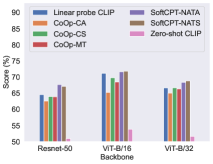
(a)

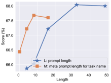
(b)

Figure 4: Results on Plant-6 with different backbones (a) and the effect with varying (meta) prompt length (b). In (a), $M$ and $K$ are set to be 8 for better performance.

Results with Different Backbones. The results with different visual encoders are shown in Fig. 4(a). SoftCPT acquires the best results with various models. Meanwhile, with ViT-B/16 and ViT-B/32 as the backbone, task-specific prompts are slightly better than task-agnostic ones.

Prompt Length and Meta Prompt Length. The curves with varying prompt length $L$ and meta prompt length $M$ for SoftCPT-NATA are shown in Fig. 4(b). With increasing lengths the score increases gradually at first and drops slightly after reaching the peak. Setting $L$ as 16 and $M$ as 8 can get a good trade-off between speed and accuracy.

Struct.	Linear	MLP(r=1)	MLP(r=2)	MLP(r=4)
Score	67.22 $\pm$ 1.11	67.15 $\pm$ 1.03	66.65 $\pm$ 1.43	66.06 $\pm$ 1.75

Table 4: Average scores (%) with different sub-network structures.

Different Sub-Networks. The effect of using different sub-networks for SoftCPT-NATA is studied. Two structures are tried: linear and MLP. For MLP, the structure is “Linear-BN-ReLU-Linear”. The first linear layer reduces the input dimension by a ratio of $r$. The results are listed in Tab. 4. It is clear that more complex sub-network does not work better than the simplest linear structure. One possible reason is that larger and deeper models are hard to fit in the few-shot setting.

Variance Reduction. We compare the Relative Standard Deviation (RSD) of different methods. Due to the normalization by mean value, RSD can eliminate the effect of varying hardness of different tasks. Here, RSD is defined as $RSD=\frac{1}{5}\sum\nolimits_{i\in\{1,2,4,8,16\}}{STD_{i}}/{Score_{i}}$, where $STD_{i}$ and $Score_{i}$ are the mean over per-task standard deviations and mean over per-task scores for the $i$-shot setting. The results on different datasets are listed in Tab. 5. We can see that SoftCPT acquires lower RSDs compared to other methods, which implies that it has more stable performance.

Method	General-10	Plant-6	Fashion-20
Linear probe CLIP	2.37	3.72	7.12
CoOp-CA	1.83	5.96	6.72
CoOp-TS	1.62	3.54	7.05
CoOp-MT	1.37	2.90	7.15
SoftCPT-NATA	1.47	3.54	5.69
SoftCPT-NATS	1.28	3.70	6.55

Table 5: Comparison of RSD (%) on three datasets.

Method	General-10 (%)	Plant-6 (%)
CoOp-CA	66.39 $\pm$ 0.52	62.59 $\pm$ 2.33
Oracle	66.46 $\pm$ 0.44	63.39 $\pm$ 1.63
EnsFeat	53.52 $\pm$ 0.40	50.38 $\pm$ 0.66
EnsPred	54.65 $\pm$ 0.31	51.27 $\pm$ 1.32
SoftCPT-NATA	67.12 $\pm$ 0.39	67.68 $\pm$ 1.18
SoftCPT-NATS	67.04 $\pm$ 0.23	67.13 $\pm$ 1.15

Table 6: Comparison to prompt transferring.

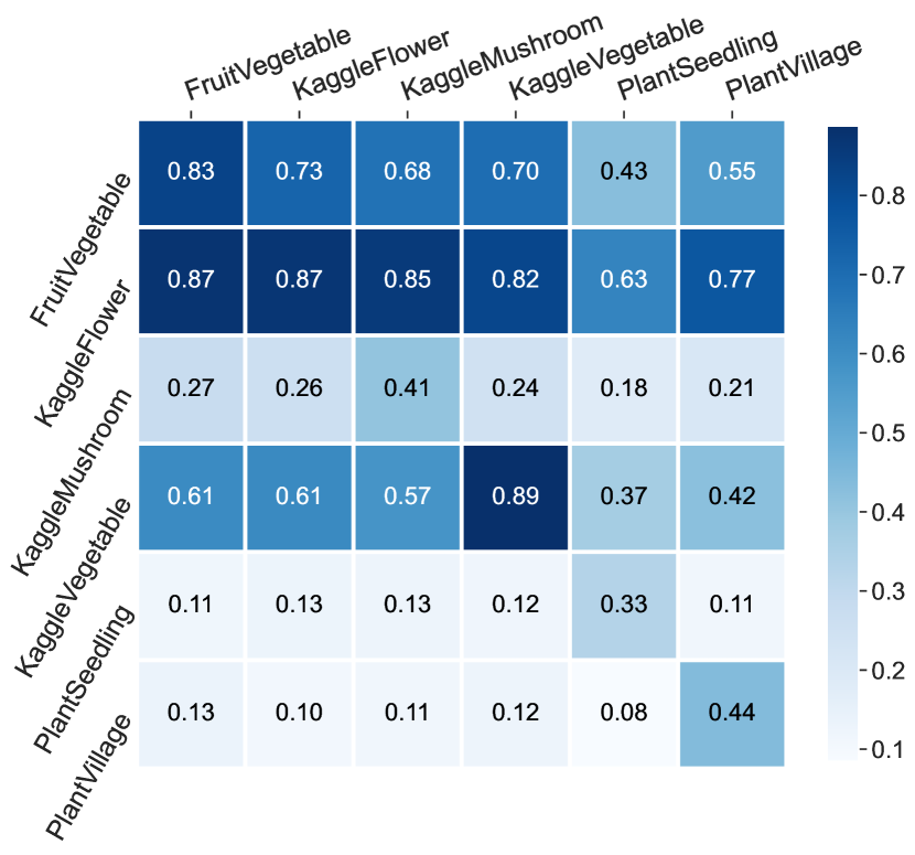
(a) $\boldsymbol{S}$

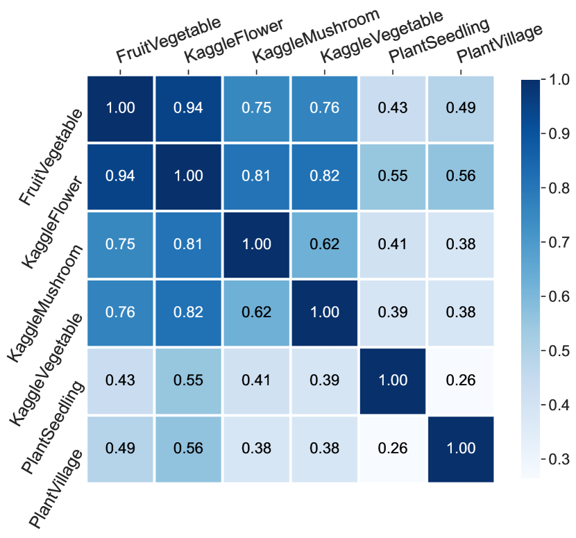
(b) $\boldsymbol{S}_{\text{oracle}}$

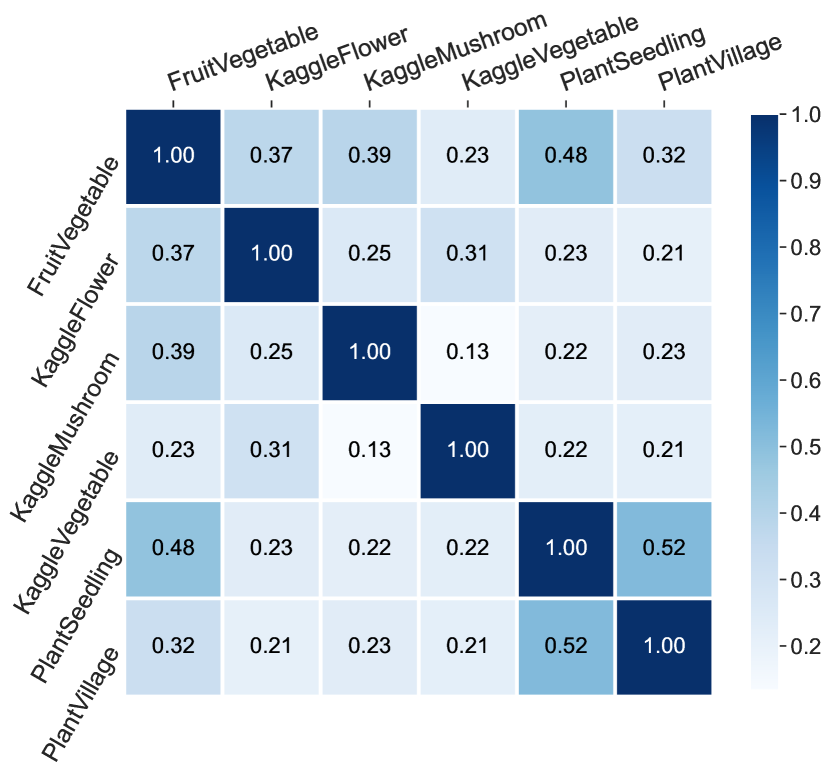
(c) $\boldsymbol{S}_{\text{st}}$

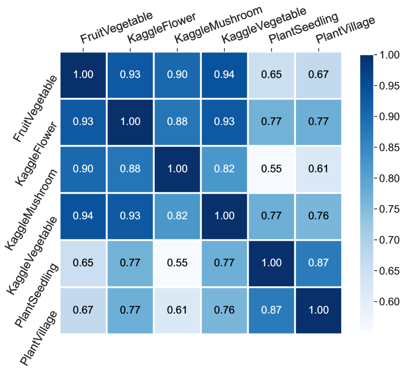
(d) $\boldsymbol{S}_{\text{mt}}$

Figure 5: Visualization of task correlation maps.

Prompt Transferring. For CoOp, we check the transferability from the prompt learned on one task to another. Transferring the prompt is also a way to exploit the relation between tasks. We compare it to our method to see if it works better than multi-task prompts. Besides, if there exists the transferability, the test set score after transferring can be seen as an indicator for evaluating the similarity/transferability between tasks. The General-10 and Plant-6 datasets are adopted here due to their few tasks. We train CoOp-CA on all $T$ (10 or 6) tasks and obtain $T$ prompt vectors. Three different transfer methods are tried: 1) Oracle computes $T$ test scores using all $T$ prompt vectors as initialization for each task, and returns the highest score as final test score for this task; 2) EnsFeat conducts an mean ensembling of $T$ classifier weights computed by using all prompt vectors as initialization and then uses the ensembled classifier for prediction; 3) EnsPred is similar to EnsFeat but the mean ensembling of prediction probabilities is used. We do not further fine-tune the prompts as this needs extra iterations compared to SoftCPT. The results are listed in Tab. 6. From the table, the following conclusions can be drawn: 1) the prompt of CoOp is transferable; 2) transferring prompts is able to improve the performance slightly (by comparing CoOp-CA and Oracle); 3) the proposed multi-task prompt learning is superior to the simple prompt transferring mentioned above; 4) the pairwise transfer score could be viewed as an good indicator of evaluating similarity/transferability between tasks due to the intuitive consistency to true task relatedness (ref. Fig. 5(a)).

Visualization. We visualize the task correlation map on Plant-6. Assume that the score matrix computed by transferring CoOp’s prompts as mentioned above is $\boldsymbol{S}$. The normalized score matrix is given by $\boldsymbol{S}^{\prime}=\boldsymbol{S}*\text{diag}(\boldsymbol{d})$, where $\text{diag}(\cdot)$ is an operator to construct diagonal matrix based on a vector, and the item of $\boldsymbol{d}$ is the inverse of the corresponding value on the diagonal position of $\boldsymbol{S}$. The symmetric task similarity matrix $\boldsymbol{S}_{\text{oracle}}$ is the mean between $\boldsymbol{S}^{\prime}$ and its transpose. Let $\boldsymbol{S}_{\text{st}}$ ($\boldsymbol{S}_{\text{mt}}$) denotes the single-task (multi-task) task similarity matrix, whose element is defined as pairwise cosine similarity between two corresponding prompt features, which are computed by encoding the prompt vectors in CoOp-CA (SoftCPT-NATA) with CLIP’s text encoder. The correlation maps are shown in Fig. 5. The coefficient between upper triangle of $\boldsymbol{S}_{\text{oracle}}$ and $\boldsymbol{S}_{\text{st}}$ is -0.03, and that between upper triangle of $\boldsymbol{S}_{\text{oracle}}$ and $\boldsymbol{S}_{\text{mt}}$ is 0.32. This means that the proposed method can better reflect the task relatedness.

5 Conclusion

This paper presents a new prompt tuning method SoftCPT for vision-language models to solve the problem of few-shot image recognition. SoftCPT learns softly-shared prompt vectors for multiple target tasks by a novel meta network. Experiments on three datasets valid the effectiveness of SoftCPT over CoOp and hard prompt sharing. The core value of our work lies in demonstrating prompts trained in multi-task manner are possible to improve performance on target tasks in the vision domain.

References

- [1] Data for: Identification of Plant Leaf Diseases Using a 9-layer Deep Convolutional Neural Network. https://data.mendeley.com/datasets/tywbtsjrjv/1. Accessed: 2022-06-03.
- [2] Flowers Recognition. https://www.kaggle.com/datasets/alxmamaev/flowers-recognition. Accessed: 2022-06-01.
- [3] Fruits and Vegetables Image Recognition Dataset. https://www.kaggle.com/datasets/kritikseth/fruit-and-vegetable-image-recognition. Accessed: 2022-06-01.
- [4] Mushrooms classification - Common genus’s images. https://www.kaggle.com/datasets/maysee/mushrooms-classification-common-genuss-images. Accessed: 2022-06-01.
- [5] Plant Seedlings Dataset. https://vision.eng.au.dk/plant-seedlings-dataset. Accessed: 2022-06-03.
- [6] Vegetable Image Dataset. https://www.kaggle.com/datasets/misrakahmed/vegetable-image-dataset. Accessed: 2022-06-02.
- [7] Akari Asai, Mohammadreza Salehi, Matthew E. Peters, and Hannaneh Hajishirzi. Attentional mixtures of soft prompt tuning for parameter-efficient multi-task knowledge sharing. CoRR, abs/2205.11961, 2022.
- [8] Lukas Bossard, Matthieu Guillaumin, and Luc Van Gool. Food-101 - mining discriminative components with random forests. In ECCV, volume 8694, pages 446–461, 2014.
- [9] Tom B. Brown, Benjamin Mann, Nick Ryder, Melanie Subbiah, Jared Kaplan, Prafulla Dhariwal, Arvind Neelakantan, Pranav Shyam, Girish Sastry, Amanda Askell, Sandhini Agarwal, Ariel Herbert-Voss, Gretchen Krueger, Tom Henighan, Rewon Child, Aditya Ramesh, Daniel M. Ziegler, Jeffrey Wu, Clemens Winter, Christopher Hesse, Mark Chen, Eric Sigler, Mateusz Litwin, Scott Gray, Benjamin Chess, Jack Clark, Christopher Berner, Sam McCandlish, Alec Radford, Ilya Sutskever, and Dario Amodei. Language models are few-shot learners. In NeurIPS, 2020.
- [10] Rich Caruana. Multi-task learning. Machine Learning, 28:41––75, 1997.
- [11] Yen-Chun Chen, Linjie Li, Licheng Yu, Ahmed El Kholy, Faisal Ahmed, Zhe Gan, Yu Cheng, and Jingjing Liu. UNITER: universal image-text representation learning. In ECCV, volume 12375, pages 104–120, 2020.
- [12] Mircea Cimpoi, Subhransu Maji, Iasonas Kokkinos, Sammy Mohamed, and Andrea Vedaldi. Describing textures in the wild. In CVPR, pages 3606–3613, 2014.
- [13] Michael Crawshaw. Multi-task learning with deep neural networks: A survey. CoRR, abs/2009.09796, 2020.
- [14] Sinuo Deng, Lifang Wu, Ge Shi, Lehao Xing, and Meng Jian. Learning to compose diversified prompts for image emotion classification. CoRR, abs/2201.10963, 2022.
- [15] Jacob Devlin, Ming-Wei Chang, Kenton Lee, and Kristina Toutanova. BERT: pre-training of deep bidirectional transformers for language understanding. In NAACL, pages 4171–4186, 2019.
- [16] Jesse Dodge, Gabriel Ilharco, Roy Schwartz, Ali Farhadi, Hannaneh Hajishirzi, and Noah A. Smith. Fine-tuning pretrained language models: Weight initializations, data orders, and early stopping. CoRR, abs/2002.06305, 2020.
- [17] Carl Doersch, Ankush Gupta, and Andrew Zisserman. CrossTransformers: spatially-aware few-shot transfer. CoRR, abs/2007.11498, 2020.
- [18] Alexey Dosovitskiy, Lucas Beyer, Alexander Kolesnikov, Dirk Weissenborn, Xiaohua Zhai, Thomas Unterthiner, Mostafa Dehghani, Matthias Minderer, Georg Heigold, Sylvain Gelly, Jakob Uszkoreit, and Neil Houlsby. An image is worth 16x16 words: Transformers for image recognition at scale. In ICLR, 2021.
- [19] Yu Du, Fangyun Wei, Zihe Zhang, Miaojing Shi, Yue Gao, and Guoqi Li. Learning to prompt for open-vocabulary object detection with vision-language model. In CVPR, pages 14084–14093, 2022.
- [20] William Fedus, Barret Zoph, and Noam Shazeer. Switch Transformers: Scaling to trillion parameter models with simple and efficient sparsity. CoRR, abs/2101.03961, 2021.
- [21] Chengjian Feng, Yujie Zhong, Zequn Jie, Xiangxiang Chu, Haibing Ren, Xiaolin Wei, Weidi Xie, and Lin Ma. PromptDet: Towards open-vocabulary detection using uncurated images. In ECCV, 2022.
- [22] Chelsea Finn, Pieter Abbeel, and Sergey Levine. Model-agnostic meta-learning for fast adaptation of deep networks. In ICML, volume 70, pages 1126–1135, 2017.
- [23] Peng Gao, Shijie Geng, Renrui Zhang, Teli Ma, Rongyao Fang, Yongfeng Zhang, Hongsheng Li, and Yu Qiao. CLIP-Adapter: Better vision-language models with feature adapters. CoRR, abs/2110.04544, 2021.
- [24] Tianyu Gao, Adam Fisch, and Danqi Chen. Making pre-trained language models better few-shot learners. In ACL-IJCNLP, pages 3816–3830, 2021.
- [25] Xiuye Gu, Tsung-Yi Lin, Weicheng Kuo, and Yin Cui. Open-vocabulary object detection via vision and language knowledge distillation. In ICLR, 2022.
- [26] Yuxian Gu, Xu Han, Zhiyuan Liu, and Minlie Huang. PPT: pre-trained prompt tuning for few-shot learning. In ACL, pages 8410–8423, 2022.
- [27] Xu Han, Zhengyan Zhang, Ning Ding, Yuxian Gu, Xiao Liu, Yuqi Huo, Jiezhong Qiu, Yuan Yao, Ao Zhang, Liang Zhang, Wentao Han, Minlie Huang, Qin Jin, Yanyan Lan, Yang Liu, Zhiyuan Liu, Zhiwu Lu, Xipeng Qiu, Ruihua Song, Jie Tang, Ji-Rong Wen, Jinhui Yuan, Wayne Xin Zhao, and Jun Zhu. Pre-trained models: Past, present and future. AI Open, 2:225–250, 2021.
- [28] Kaiming He, Xiangyu Zhang, Shaoqing Ren, and Jian Sun. Deep residual learning for image recognition. CoRR, abs/1512.03385, 2015.
- [29] Patrick Helber, Benjamin Bischke, Andreas Dengel, and Damian Borth. EuroSAT: A novel dataset and deep learning benchmark for land use and land cover classification. IEEE J. Sel. Top. Appl. Earth Obs. Remote. Sens., 12(7):2217–2226, 2019.
- [30] Neil Houlsby, Andrei Giurgiu, Stanislaw Jastrzebski, Bruna Morrone, Quentin de Laroussilhe, Andrea Gesmundo, Mona Attariyan, and Sylvain Gelly. Parameter-efficient transfer learning for NLP. In ICML, volume 97, pages 2790–2799, 2019.
- [31] Jeremy Howard and Sebastian Ruder. Universal language model fine-tuning for text classification. In ACL, pages 328–339, 2018.
- [32] Chao Jia, Yinfei Yang, Ye Xia, Yi-Ting Chen, Zarana Parekh, Hieu Pham, Quoc V. Le, Yun-Hsuan Sung, Zhen Li, and Tom Duerig. Scaling up visual and vision-language representation learning with noisy text supervision. In ICML, volume 139, pages 4904–4916, 2021.
- [33] Haoming Jiang, Pengcheng He, Weizhu Chen, Xiaodong Liu, Jianfeng Gao, and Tuo Zhao. SMART: robust and efficient fine-tuning for pre-trained natural language models through principled regularized optimization. In ACL, pages 2177–2190, 2020.
- [34] Zhengbao Jiang, Frank F. Xu, Jun Araki, and Graham Neubig. How can we know what language models know. Trans. Assoc. Comput. Linguistics, 8:423–438, 2020.
- [35] Shibo Jie and Zhi-Hong Deng. Convolutional bypasses are better vision transformer adapters. CoRR, abs/2207.07039, 2022.
- [36] Alex Kendall, Yarin Gal, and Roberto Cipolla. Multi-task learning using uncertainty to weigh losses for scene geometry and semantics. In CVPR, pages 7482–7491, 2018.
- [37] Daniel Khashabi, Xinxi Lyu, Sewon Min, Lianhui Qin, Kyle Richardson, Sean Welleck, Hannaneh Hajishirzi, Tushar Khot, Ashish Sabharwal, Sameer Singh, and Yejin Choi. Prompt waywardness: The curious case of discretized interpretation of continuous prompts. In NAACL, pages 3631–3643, 2022.
- [38] Wonjae Kim, Bokyung Son, and Ildoo Kim. ViLT: Vision-and-language transformer without convolution or region supervision. In ICML, volume 139, pages 5583–5594, 2021.
- [39] Jonathan Krause, Michael Stark, Jia Deng, and Li Fei-Fei. 3D object representations for fine-grained categorization. In ICCVW, pages 554–561, 2013.
- [40] Ananya Kumar, Aditi Raghunathan, Robbie Jones, Tengyu Ma, and Percy Liang. Fine-tuning can distort pretrained features and underperform out-of-distribution. CoRR, abs/2202.10054, 2022.
- [41] Gihyun Kwon and Jong Chul Ye. CLIPstyler: Image style transfer with a single text condition. In CVPR, pages 18062–18071, 2022.
- [42] Brian Lester, Rami Al-Rfou, and Noah Constant. The power of scale for parameter-efficient prompt tuning. In EMNLP, pages 3045–3059, 2021.
- [43] Fei-Fei Li, Robert Fergus, and Pietro Perona. One-shot learning of object categories. IEEE Trans. Pattern Anal. Mach. Intell., 28(4):594–611, 2006.
- [44] Fei-Fei Li, Robert Fergus, and Pietro Perona. Learning generative visual models from few training examples: An incremental bayesian approach tested on 101 object categories. Comput. Vis. Image Underst., 106(1):59–70, 2007.
- [45] Gen Li, Nan Duan, Yuejian Fang, Ming Gong, and Daxin Jiang. Unicoder-VL: A universal encoder for vision and language by cross-modal pre-training. In AAAI, pages 11336–11344, 2020.
- [46] Liunian Harold Li, Mark Yatskar, Da Yin, Cho-Jui Hsieh, and Kai-Wei Chang. VisualBERT: A simple and performant baseline for vision and language. CoRR, abs/1908.03557, 2019.
- [47] Xiang Lisa Li and Percy Liang. Prefix-Tuning: Optimizing continuous prompts for generation. In ACL-IJCNLP, pages 4582–4597, 2021.
- [48] Xiao Liu, Yanan Zheng, Zhengxiao Du, Ming Ding, Yujie Qian, Zhilin Yang, and Jie Tang. GPT understands, too. CoRR, abs/2103.10385, 2021.
- [49] Ze Liu, Yutong Lin, Yue Cao, Han Hu, Yixuan Wei, Zheng Zhang, Stephen Lin, and Baining Guo. Swin Transformer: Hierarchical vision transformer using shifted windows. In ICCV, 2021.
- [50] Jiasen Lu, Dhruv Batra, Devi Parikh, and Stefan Lee. ViLBERT: Pretraining task-agnostic visiolinguistic representations for vision-and-language tasks. In NeurIPS, pages 13–23, 2019.
- [51] Yuning Lu, Jianzhuang Liu, Yonggang Zhang, Yajing Liu, and Xinmei Tian. Prompt distribution learning. In CVPR, pages 5206–5215, 2022.
- [52] Timo Lüddecke and Alexander Ecker. Image segmentation using text and image prompts. In CVPR, pages 7086–7096, 2022.
- [53] Subhransu Maji, Esa Rahtu, Juho Kannala, Matthew B. Blaschko, and Andrea Vedaldi. Fine-grained visual classification of aircraft. CoRR, abs/1306.5151, 2013.
- [54] Ron Mokady, Amir Hertz, and Amit H. Bermano. ClipCap: CLIP prefix for image captioning. CoRR, abs/2111.09734, 2021.
- [55] Norman Mu, Alexander Kirillov, David A. Wagner, and Saining Xie. SLIP: self-supervision meets language-image pre-training. CoRR, abs/2112.12750, 2021.
- [56] Maria-Elena Nilsback and Andrew Zisserman. Automated flower classification over a large number of classes. In ICVGIP, pages 722–729, 2008.
- [57] Omkar M. Parkhi, Andrea Vedaldi, Andrew Zisserman, and C. V. Jawahar. Cats and dogs. In CVPR, pages 3498–3505, 2012.
- [58] Guanghui Qin and Jason Eisner. Learning how to ask: Querying LMs with mixtures of soft prompts. In NAACL, pages 5203–5212, 2021.
- [59] Yujia Qin, Xiaozhi Wang, YuSheng Su, Yankai Lin, Ning Ding, Zhiyuan Liu, Juanzi Li, Lei Hou, Peng Li, Maosong Sun, and Jie Zhou. Exploring low-dimensional intrinsic task subspace via prompt tuning. CoRR, abs/2110.07867, 2021.
- [60] Alec Radford, Jong Wook Kim, Chris Hallacy, Aditya Ramesh, Gabriel Goh, Sandhini Agarwal, Girish Sastry, Amanda Askell, Pamela Mishkin, Jack Clark, Gretchen Krueger, and Ilya Sutskever. Learning transferable visual models from natural language supervision. In ICML, volume 139, pages 8748–8763, 2021.
- [61] Colin Raffel, Noam Shazeer, Adam Roberts, Katherine Lee, Sharan Narang, Michael Matena, Yanqi Zhou, Wei Li, and Peter J. Liu. Exploring the limits of transfer learning with a unified text-to-text transformer. JMLR, 21:140:1–140:67, 2020.
- [62] Yongming Rao, Wenliang Zhao, Guangyi Chen, Yansong Tang, Zheng Zhu, Guan Huang, Jie Zhou, and Jiwen Lu. DenseCLIP: Language-guided dense prediction with context-aware prompting. In CVPR, pages 18082–18091, 2022.
- [63] Andreas Rücklé, Gregor Geigle, Max Glockner, Tilman Beck, Jonas Pfeiffer, Nils Reimers, and Iryna Gurevych. AdapterDrop: On the efficiency of adapters in transformers. In EMNLP, pages 7930–7946, 2021.
- [64] Aditya Sanghi, Hang Chu, Joseph G. Lambourne, Ye Wang, Chin-Yi Cheng, and Marco Fumero. CLIP-Forge: Towards zero-shot text-to-shape generation. CoRR, abs/2110.02624, 2021.
- [65] Taylor Shin, Yasaman Razeghi, Robert L. Logan IV, Eric Wallace, and Sameer Singh. AutoPrompt: Eliciting knowledge from language models with automatically generated prompts. In EMNLP, pages 4222–4235, 2020.
- [66] Amanpreet Singh, Ronghang Hu, Vedanuj Goswami, Guillaume Couairon, Wojciech Galuba, Marcus Rohrbach, and Douwe Kiela. FLAVA: A foundational language and vision alignment model. CoRR, abs/2112.04482, 2021.
- [67] Jake Snell, Kevin Swersky, and Richard S. Zemel. Prototypical networks for few-shot learning. In NeurIPS, pages 4077–4087, 2017.
- [68] Khurram Soomro, Amir Roshan Zamir, and Mubarak Shah. UCF101: A dataset of 101 human actions classes from videos in the wild. CoRR, abs/1212.0402, 2012.
- [69] Yusheng Su, Xiaozhi Wang, Yujia Qin, Chi-Min Chan, Yankai Lin, Huadong Wang, Kaiyue Wen, Zhiyuan Liu, Peng Li, Juanzi Li, Lei Hou, Maosong Sun, and Jie Zhou. On transferability of prompt tuning for natural language processing. In NAACL, pages 3949–3969, 2022.
- [70] Ximeng Sun, Ping Hu, and Kate Saenko. DualCoOp: Fast adaptation to multi-label recognition with limited annotations. CoRR, abs/2206.09541, 2022.
- [71] Yi-Lin Sung and Jaemin Cho andMohit Bansal. VL-Adapter: Parameter-efficient transfer learning for vision-and-language tasks. In CVPR, pages 5227–5237, 2022.
- [72] Yonglong Tian, Yue Wang, Dilip Krishnan, Joshua B. Tenenbaum, and Phillip Isola. Rethinking few-shot image classification: A good embedding is all you need? In ECCV, volume 12359, pages 266–282, 2020.
- [73] Ashish Vaswani, Noam Shazeer, Niki Parmar, Jakob Uszkoreit, Llion Jones, Aidan N. Gomez, Lukasz Kaiser, and Illia Polosukhin. Attention is all you need. In NeurIPS, pages 5998–6008, 2017.
- [74] Jianxiong Xiao, James Hays, Krista A. Ehinger, Aude Oliva, and Antonio Torralba. SUN database: Large-scale scene recognition from abbey to zoo. In CVPR, pages 3485–3492, 2010.
- [75] Lewei Yao, Runhui Huang, Lu Hou, Guansong Lu, Minzhe Niu, Hang Xu, Xiaodan Liang, Zhenguo Li, Xin Jiang, and Chunjing Xu. FILIP: Fine-grained interactive language-image pre-training. In ICLR, 2022.
- [76] Tianyi Zhang, Felix Wu, Arzoo Katiyar, Kilian Q. Weinberger, and Yoav Artzi. Revisiting few-sample BERT fine-tuning. In ICLR, 2021.
- [77] Kaiyang Zhou, Jingkang Yang, Chen Change Loy, and Ziwei Liu. Conditional prompt learning for vision-language models. In CVPR, pages 16816–16825, 2022.
- [78] Kaiyang Zhou, Jingkang Yang, Chen Change Loy, and Ziwei Liu. Learning to prompt for vision-language models. IJCV, 130(9):2337–2348, 2022.