Joint Learning Content and Degradation Aware Embedding for Blind Super-Resolution

Abstract.

To achieve promising results on blind image super-resolution (SR), some attempts leveraged the low resolution (LR) images to predict the kernel and improve the SR performance. However, these Supervised Kernel Prediction (SKP) methods are impractical due to the unavailable real-world blur kernels. Although some Unsupervised Degradation Prediction (UDP) methods are proposed to bypass this problem, the inconsistency between degradation embedding and SR feature is still challenging. By exploring the correlations between degradation embedding and SR feature, we observe that jointly learning the content and degradation aware feature is optimal. Based on this observation, a Content and Degradation aware SR Network dubbed CDSR is proposed. Specifically, CDSR contains three newly-established modules: (1) a Lightweight Patch-based Encoder (LPE) is applied to jointly extract content and degradation features; (2) a Domain Query Attention based module (DQA) is employed to adaptively reduce the inconsistency; (3) a Codebook-based Space Compress module (CSC) that can suppress the redundant information. Extensive experiments on several benchmarks demonstrate that the proposed CDSR outperforms the existing UDP models and achieves competitive performance on PSNR and SSIM even compared with the state-of-the-art SKP methods.

1. Introduction

Figure 1. Some SR results for scale factor of $\times 4$. Existing methods produce artifacts due to they apply the moderate receptive field (MANet (Liang et al., 2021)), implicit content-aware degradation embedding (DASR (Wang et al., 2021)). We introduce the content information as the cue to enhance the cooperation between degradation embedding and the SR network.

Blind image super-resolution aims to restore high-resolution images from low resolution inputs with unknown degradation factors. Unlike single image super-resolution (SISR) methods (Dong et al., 2014; Zhang et al., 2018b; Dong et al., 2016; Wang et al., 2018; Singh et al., 2014) which are developed based on a pre-defined degradation process (e.g., bicubic downsampling). Blind SR towards higher generalization and practicability. Usually, blind SR is achieved by two steps: degradation estimation within the prior encoder, and the fusion of degradation prior and textural features within the SR network. Based on the designs of degradation extraction, existing blind SR approaches can be divided into two groups:

(1) Supervised Kernel Prediction (SKP). Most existing works (Gu et al., 2019; Huang et al., 2020; Liang et al., 2021; Zhang et al., 2018d, 2021a; Tao et al., 2021; Zhang et al., 2020; Kim et al., 2021) employ the classical degradation model to represent the degradation. Previous SKP methods leverage explicit (Gu et al., 2019; Kim et al., 2021; Abu Hussein et al., 2020; Zhang et al., 2018d; Soh et al., 2020; Zhang et al., 2020) or implicit (Bell-Kligler et al., 2019; Luo et al., 2022) ways to predict blur kernels, and then employ the kernel stretching strategy to provide the degradation information for non-blind SR networks. However, SKP methods are impractical due to the real-world kernels are unavailable. Once given complex degradation deviating from their training distribution, these methods inevitably lead to inferior results. Furthermore, SKP can only handle the blur kernel-based degradation, and cannot be extended to other degradation (e.g., noise).

(2) Unsupervised Degradation Prediction (UDP). Unlike the SKP methods that only consider kernel degradation, UDP (Wang et al., 2021; Zhang et al., 2021b) has developed a more suitable manner for real-world applications with unknown degradation. Instead of requiring supervision from the ground-truth kernel label, UDP leverages the degradation embedding which can naturally avoid the drawback of SKP. Besides, the degradation embedding learned in UDP can be applied to represent not only the blur kernel but also other degradations (e.g., noise). As the most representative approach, DASR (Wang et al., 2021) investigates the degradation representation in an unsupervised manner through contrastive learning. Although DASR has outperformed some SKP methods (Gu et al., 2019; Bell-Kligler et al., 2019) within the easy degradation, there is still a gap between DASR and the latest SKP (Liang et al., 2021; Luo et al., 2022) in more complex scenarios.

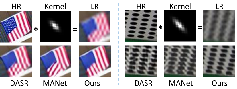
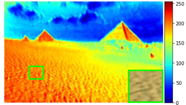
Towards achieving a more effective and competitive UDP, we firstly investigate the key point on: What kind of degradation embedding is really needed for SR networks? Surprisingly, we observed that using a degradation-oriented embedding will fail to improve the network performance or even end up with poor results, more details in Sec. 3. Based on the inverse-U relationship between classification accuracy and content information claimed in (Kumar et al., 2022), a reasonable explanation is that in order to classify the degradation, the encoder only preserves the degradation-related feature and ignores the content information. As mentioned in (Wang et al., 2021; Gu et al., 2019), the straightforward interaction between degradation space and content space will introduce interference. Without explicitly considering the content information, the degradation-oriented embedding is agnostic to the textural information which serves the SR network and then results in the artifacts, shown in Fig. 1.

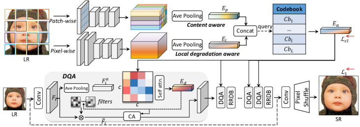
In this work, we polish the UDP method through three aspects, and then produce more promising results: (1) Since the content information can serve as the cue for the SR network, we derive that content-aware degradation helps address the interference from the domain gap between degradation and content spaces. The previous methods which only employ a small receptive field or naive encoder may be stumbled by the inconsistency between the above two spaces because these embeddings do not make full use of the content information. Inspired by the recent patch-based transformers (Dosovitskiy et al., 2021; Trockman and Kolter, 2022), we propose a Lightweight Patch-based Encoder (LPE) to extract both the content and degradation aware features. The LPE not only promotes the extraction of content information but also introduces the patch degradation consistency, thus being more competitive to model the global degradation. (2) To adaptively fuse the predicted embedding into the SR network, we propose Domain Query Attention based module (DQA) to achieve the content-aware fusion. (3) Moreover, as claimed in (Gu et al., 2019), using PCA to project the kernel representation to low-dimension can make the network easier to learn the relationship between degradation and SR. However, PCA can not be trained end-to-end with SR network, thus failing to learn the adaptive degradation embedding. We extend this and introduce a Codebook-based Space Compress module (CSC) to limit the basis of feature space, thus reducing redundancy.

Specifically, we propose a Content and Degradation Aware SR Network, termed CDSR, which enhances the UDP based blind SR by narrowing the domain gap between degradation embedding and SR content feature. Extensive experiments show that the proposed CDSR outperforms the existing UDP models and achieves competitive performance on PSNR and SSIM even compared with the SOTA SKP methods. The main contributions of this paper are as follows:

• We first analyze the relation between content information and degradation embedding. Based on this, we proposed a lightweight patch-based encoder (LPE) to extract content-aware degradation embedding features.

• We present a Domain Query Attention based module (DQA) to adaptively fuse the predicted content and degradation aware embedding into the SR network.

• Inspired by PCA, we introduce a Codebook-based Space Compress module (CSC) to limit the basis of feature space.

2. Related Work

2.1. Non-blind SR

Since SRCNN (Dong et al., 2014) was first proposed to learn the mapping from LR to HR, the booming deep learning techniques are widely applied to SISR. Various elaborate network architectures (Dong et al., 2016; Ledig et al., 2017; Dai et al., 2019; Haris et al., 2018; Zhang et al., 2018c; Kim et al., 2016a, b; Wang et al., 2018; Tai et al., 2017a, b) and complex loss functions (Johnson et al., 2016; Lugmayr et al., 2020; Zhang et al., 2018a) are then proposed. Following the residual design, Kim et al.  (Kim et al., 2016a) propose a deep residual SR network. Besides the residual learning strategy, Zhang et al.  (Zhang et al., 2018c) apply the channel-wise attention. Dai et al.  (Dai et al., 2019) introduce the second-order version to achieve promising results. Kim et al.  (Kim et al., 2016b) employ the DRCN to recursively refine the extraction feature. However, these approaches are developed based on a pre-defined degradation process (e.g., bicubic downsampling), which can hardly hold true when applied to real-world images. Given more complex degradation deviating from their assumed type, these methods inevitably lead to inferior results. To be more flexible, some SR networks are designed to address different degradations with given corresponding priority. Specifically, Wang et al.  (Wang et al., 2018) achieve impressive results by considering the textural information in the SR network and introducing the SFT layer. Later, SRMD (Zhang et al., 2018d) takes the degradation as the additional input to super-resolve LR images under different kernels. Xu et al.  (Xu et al., 2020) incorporate dynamic convolution to achieve more flexible alternative. Although the above approaches achieve promising results, the kernels (i.e., priorities) are not available when extended to real-world images.

2.2. Blind SR

Supervised Kernel Prediction. In order to polish the non-blind SR networks, some attempts are leveraged to estimate the kernels, then employing some adaptive fusion strategies (e.g., AdaIN (Huang and Belongie, 2017; Wang et al., 2018), kernel stretching (Zhang et al., 2018d), dynamic blocks  (Jia et al., 2016)). The non-blind SR networks are sensitive to the kernel information consequently the optimal kernel estimation is important. Gu et al.  (Gu et al., 2019) proposed iterative kernel correction (IKC) to refine the predicted kernel progressively by observing the previous SR results. Furthermore, DAN  (Luo et al., 2021) has unfolded the previous iterating process into an end-to-end manner by corporately using the Restorer and Estimator and yields better results. MANet  (Liang et al., 2021) leverages moderate receptive field and exploits channel interdependence to conduct the kernel estimation. KOALANet  (Kim et al., 2021) employs the pixel-wised local kernels and dynamic filter to integrate kernel information for SR. Later, Luo et al.  (Luo et al., 2022) propose DCLS module to generate clean features based on the reformulation and estimated kernel. These methods can achieve remarkable performance when given the ground-truth blur kernel. However, in the real-world images, the blur kernels predicted by kernel-estimating methods deviate from those of the ground-truth. SKP methods are sensitive to kernel estimation and cannot be extended to other degradations.

Unsupervised Degradation Prediction. UDP has developed a more suitable manner for real-world applications with unknown degradation. Instead of requiring the supervision from the ground-truth kernel label, UDP leverages the degradation embedding which can naturally avoid the drawback of SKP. Wang et al. firstly propose DASR (Wang et al., 2021) to achieve unsupervised degradation prediction, using contrastive loss for unsupervised degradation representation learning. In order to improve the contrastive learning procedure, Zhang et al.  (Zhang et al., 2021b) introduce CRL-SR to extract refined contrastive features via a bidirectional contrastive loss. However, previous UDP approaches pay little attention to what kind of degradation embedding is really needed for blind SR. In fact, they ignore that discriminative embedding which lacks content features will cause the problem of domain gap (Gu et al., 2019). Instead, our proposed LPE jointly learns the content and degradation aware embedding, thus achieving promising results. Besides, DQA can leverage the content feature to query the adaptive embedding feature for the SR network.

2.3. Contrastive Learning

Contrastive learning is prevalently studied for unsupervised representation learning. Several recent studies (Chen et al., 2020; Tian et al., 2020; Noroozi et al., 2017; He et al., 2020) present promising results by minimizing the distance of similar tokens meanwhile maximizing that of dissimilar ones. Specifically, some of the UDP methods leverage the contrastive learning approaches to distinguish the latent degradation from other ones. However, to classify the degradation, the encoder only preserves the degradation-related feature and ignores the content information therefore introducing the problem of domain gap. Although, previous methods have applied the effective contrastive learning approaches (He et al., 2020) to enrich the learning samples, there is also the redundancy between different degradations. The proposed CSC can alleviate this by limiting the basis of feature space.

Table 1. Classification accuracy of degradation embedding and PSNR of $\times 4$ SR. We choose the positive sample in three different ways. ‘C&D’: cropped from the same image with the same degradation (used in DASR). ‘D’: cropped from different images with the same degradation. ‘C’: cropped from the same image but with different degradation. More discriminative embedding fails to achieve higher PSNR.

Positive	Acc.	Set5	Set14	B100	U100
C&D	75.40%	31.45 dB	28.12 dB	27.24 dB	25.28 dB
D	80.80%	31.36 dB	28.03 dB	27.20 dB	25.12 dB
C	12.00%	31.32 dB	28.06 dB	27.24 dB	25.26 dB

3. Analysis on Degradation Embedding

The Higher Degradation Accuracy the Better? We firstly investigate the key point on: What kind of degradation embedding is really needed for SR networks? As shown in Table 1, we conduct three experiments based on the SOTA DASR (Wang et al., 2021) to further investigate the learned degradation representation. In Table 1, we show the effect of content information by only changing the positive selection strategy during contrastive learning.

Given $100$ images from B$100$ (Martin et al., 2001) and the pre-trained encoder $E(\cdot)$. Each HR is degraded by $10$ different degradations to obtain the LR, using Anisotropic Gaussian kernels with $\sigma_{1}=\sigma_{2}\in[1,10]$ and $\theta$ as $0$. The scale factor is $\times 4$. The average of $50$ sampled LR embedding from the same degradation is regarded as the cluster center $D$. The rest of $50$ LR images $I$ are utilized to test the accuracy of classification, which can be mathematically calculated by:

(1) $$Acc.=\frac{\sum_{i,j}Sign\{\arg\max_{k}(Sim(E(I_{i}^{j}),D_{k})),j\}}{N},$$

where $i\in[1,50]$, $j,k\in[1,10]$, $N=500$, $I_{i}^{j}$ denotes $i^{th}$ image which is degraded by $\sigma_{1}=\sigma_{2}=j$, $D_{k}$ denotes the $k^{th}$ cluster center, and $Sign(x,y)=1$ when $x=y$; $Sign(x,y)=0$ when $x\neq y$, the $Sim(x,y)$ calculates the cosine similarity of $x$ and $y$. The accuracy denotes the encoder’s capability of degradation classification. In DASR  (Wang et al., 2021), patches from the same image with the same degradation are considered as positive samples, while different degradations as negative counterparts, as shown in the first row of Table 1. Based on contrastive learning, the encoder in DASR can capture the degradation information and implicitly learn the content information.

To enhance the capability of degradation classify (second row of Table 1), the network is constrained to focus on the degradation by discarding the implicit content information within patches from a single image. Although it can achieve higher classification accuracy, the PSNR drops. The reason may be the encoder only preserves the degradation-related feature and ignores the content information, as demonstrated in (Kumar et al., 2022) that there exists an inverse-U relationship between classify accuracy and content information. Lacking content information introduces the domain gap between embedding and textural spaces, resulting in poor SR performance.

DASR	Ours

Figure 2. Top: Representations for embedding with different blur kernels (denoted in colors). Bottom: SR Feature visualization. DASR pays more attention to local degradation. However, CDSR jointly learns the content and degradation aware embedding to achieve better results. $0\sim 255$ denotes the active intensity of the feature map.

Figure 3. Top: Lightweight Patch-based Encoder (LPE) and Codebook-based Space Compression module (CSC). LPE includes patch-wise feature extraction and pixel-wise feature extraction. Bottom: SR network composed of proposed DQAs. The output content and degradation aware embedding $\bm{E_{a}}$ is utilized in each DQA to adaptively produce dynamic filters. Self-attention and channel attention modules (CA) are also applied in DQA to help improve performance.

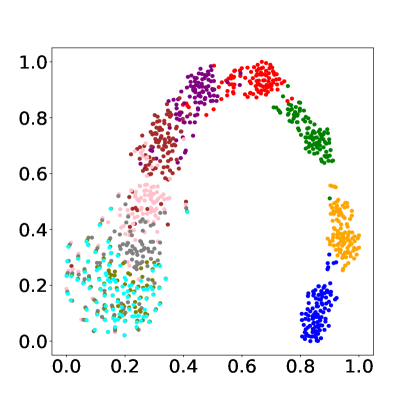
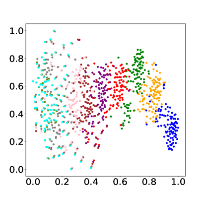
Effect of Content-aware Embedding. We then conduct the experiment where patches from the same image but different degradations are regarded as positive counterparts, the third row of Table 1. Surprisingly, although the classification accuracy only occupies 12%, it can achieve promising PSNR results, especially in the tough test sets i.e., B$100$ and U$100$. Conclusively, the content information can narrow the domain gap between degradation and textural spaces. When the encoder is guided to extract the degradation embedding meanwhile preserving the content information, it can produce the most suitable embedding for the SR network. We use the t-SNE (Hinton and Roweis, 2002) to visualize the embedding space (see Fig. 2). DASR produces better degradation classification results with larger inter distance but finally gets blurry results compared to our CDSR, which pays more attention on content information (e.g., pyramid and sand). It indicates that more explicit content features might slightly disturb degradation classification. However, it can serve as a cue to recover complex textures and boost SR performance.

4. Proposed Method

4.1. Lightweight Patch-based Encoder

Unlike previous approaches (Wang et al., 2021; Liang et al., 2021) that employ the naive or small receptive field encoder, we introduce the Lightweight Patch-based Encoder (LPE) to produce the content and degradation aware embedding. LPE has two sub-modules which are designed to extract corresponded content and local degradation-aware features:

Patch-wise Feature Extraction. Inspired by the patch-based vision transformers (Dosovitskiy et al., 2021; Trockman and Kolter, 2022), a simple lightweight patch-based encoder is designed to fast expand the receptive field of convolution and extract the content information. Specifically, the patch embedding layer is utilized to replace the first standard convolution layer. Then, the output patch feature $F_{p}\in\mathbb{R}^{\frac{H}{P}\times\frac{W}{P}\times C}$ is processed by several standard convolution layers. Finally, we average the $F_{p}$ within the spatial dimension to get $E_{p}$.

Pixel-wise Feature Extraction. As claimed in (Liang et al., 2021), a moderate receptive field can help the network to estimate the blur kernel. Hence, the receptive field of this sub-module is fixed to a moderate range and then extracts the local degradation-related information. Finally, the output is averaged to obtain $E_{l}$.

4.2. Codebook-based Space Compression

The previous SKP usually employs PCA for the reduction of feature space. More experiments results (Gu et al., 2019; Zhang et al., 2018d) demonstrated that instead of directly using the kernel, the stretched kernel representation can make it easier for the network to learn the relationship between degradation and SR. To extend this advantage in UDP, we propose the Codebook-based Space Compression module (CSC). The inclusion relationship in degradation introduces redundancy and expands the domain gap between degradation and SR feature space. After feature extraction, the CSC is utilized to constrict the basis of embedding space. Mathematically, this procedure can be described as:

(2) $$\bm{Q_{e}} =MLP(Cat(\bm{E_{p}},\bm{E_{l}})),$$

$$\bm{K_{e}} =MLP(\bm{Cb}),$$

$$\bm{E_{a}} =softmax(\bm{Q_{e}}\cdot\bm{K_{e}}^{T})\cdot\bm{Cb},$$

where $\bm{Cb}\in\mathbb{R}^{L\times C}$ denotes the codebook, $L$ denotes the length of codebook, and $C$ is the channel number of embedding.

Table 2. Quantitative comparison on different test sets with anisotropic Gaussian kernels. The best two results are highlighted in red and blue colors, respectively. The supervised tag denotes whether the corresponding method belongs to SKP or UDP.

Method	Scale Factor	Noise Level	Supervised	Set5	Set14	BSD100	Urban100
SRSVD (Cornillere et al., 2019)	$\times 2$	0	✓	34.51/0.8787	31.10.0.8581	29.71/0.7993	28.08/0.7965
IKC (Gu et al., 2019)	$\times 2$	0	✓	35.30/0.9381	31.48/0.8797	30.50/0.8545	28.62/0.8689
MANet (Liang et al., 2021)	$\times 2$	0	✓	35.98/0.9420	31.95 /0.8845	30.97 /0.8651	29.61/0.8880
1-8[3pt/2.5pt] HAN (Niu et al., 2020)	$\times 2$	0	✕	26.83/0.7919	23.21/0.6888	25.11/0.6613	22.42/0.6571
DIP (Ulyanov et al., 2018)	$\times 2$	0	✕	28.19/0.7939	25.66/0.6999	25.03/0.6762	22.97/0.6737
KernelGAN + ZSSR (Bell-Kligler et al., 2019)	$\times 2$	0	✕	-	23.92/0.6898	25.28/0.6395	21.97/0.6582
HAN + Correction (Hussein et al., 2020)	$\times 2$	0	✕	28.61/0.8013	26.22/0.7292	26.88/0.7116	25.31/0.7109
DASR (Wang et al., 2021)	$\times 2$	0	✕	35.30/0.9360	31.30/0.8683	30.46/0.8507	28.66/0.8654
Ours	$\times 2$	0	✕	36.17/0.9428	32.14 /0.8841	31.02 /0.8643	29.57/0.8851
IKC (Gu et al., 2019)	$\times 3$	0	✓	32.94/0.9104	29.14/0.8162	28.36/0.7814	26.34/0.8049
MANet (Liang et al., 2021)	$\times 3$	0	✓	33.69/0.9184	29.81/0.8270	28.81 /0.7932	27.39 /0.8331
1-8[3pt/2.5pt] HAN (Niu et al., 2020)	$\times 3$	0	✕	23.71/0.6171	22.31/0.5878	23.21/0.5653	20.34/0.5311
DIP (Ulyanov et al., 2018)	$\times 3$	0	✕	27.51/0.7740	25.03/0.6674	24.60/0.6499	22.23/0.6450
DASR (Wang et al., 2021)	$\times 3$	0	✕	33.43/0.9151	29.57/0.8187	28.58/0.7846	26.83/0.8174
Ours	$\times 3$	0	✕	33.81/0.9192	29.95/0.8275	28.81 /0.7922	27.44 /0.8329
IKC (Gu et al., 2019)	$\times 4$	0	✓	31.08/0.8781	27.83/0.7663	27.12/0.7233	25.16/0.7609
MANet (Liang et al., 2021)	$\times 4$	0	✓	31.54/0.8876	28.28/0.7727	27.36/0.7307	25.66/0.7760
1-8[3pt/2.5pt] HAN (Niu et al., 2020)	$\times 4$	0	✕	21.71/0.5941	20.42/0.4937	21.48/0.4901	19.01/0.4676
DIP (Ulyanov et al., 2018)	$\times 4$	0	✕	26.71/0.7417	24.52/0.6360	24.34/0.6160	21.85/0.6155
KernelGAN + ZSSR (Bell-Kligler et al., 2019)	$\times 4$	0	✕	-	-	18.24/0.3689	16.80/0.3960
HAN + Correction (Hussein et al., 2020)	$\times 4$	0	✕	24.31/0.6357	24.44/0.6341	24.01/0.6005	22.32/0.6368
DASR (Wang et al., 2021)	$\times 4$	0	✕	31.45/0.8859	28.12/0.7703	27.24/0.7284	25.28/0.7636
Ours	$\times 4$	0	✕	31.63/0.8885	28.31/0.7746	27.38/0.7311	25.75/0.7783
IKC (Gu et al., 2019)	$\times 4$	15	✓	27.23/0.7877	25.55/0.6717	25.15/0.6236	23.31/0.6697
MANet (Liang et al., 2021)	$\times 4$	15	✓	27.58/0.7915	25.75/0.6744	25.30/0.6262	23.57/0.6760
1-8[3pt/2.5pt] HAN (Niu et al., 2020)	$\times 4$	15	✕	20.88/0.4245	18.91/0.2901	21.01/0.4881	19.31/0.3552
DIP (Ulyanov et al., 2018)	$\times 4$	15	✕	18.60/0.2695	18.14/0.2392	17.90/0.2073	18.82/0.3476
KernelGAN + ZSSR (Bell-Kligler et al., 2019)	$\times 4$	15	✕	-	-	19.56/0.4582	13.65/0.1136
HAN + Correction (Hussein et al., 2020)	$\times 4$	15	✕	19.21/0.2281	18.21/0.2478	19.25/0.4231	19.01/0.3500
DASR (Wang et al., 2021)	$\times 4$	15	✕	27.48/0.7907	25.56/0.6723	25.25/0.6261	23.30/0.6663
Ours	$\times 4$	15	✕	27.70/0.7947	25.81/0.6757	25.33/0.6277	23.60/0.6761

4.3. Domain Query Attention based Module

Existing methods usually fuse embeddings into non-blind SR networks without considering the domain gap. The degradation features are different from the textural features which propagate in the SR network. Therefore, we propose the Domain Query Attention based module to mitigate the domain gap. Since $\bm{E_{a}}$ contains the content information, an intuitive solution is to leverage content cue to query the target value in $\bm{E_{a}}$. Generally, each DQA employs the self-attention module to attend the embedding based on the current input feature $\bm{F_{i}}$. Specifically, we first average the $\bm{F_{i}}$ within the spatial dimension to get $\bm{F_{i}^{a}}\in\mathbb{R}^{C\times 1}$. Then, the channel-wise mutual self-attention is conducted in the DQA:

(3) $$Attention(\bm{Q_{d}},\bm{K},\bm{V})=softmax(\frac{\bm{Q_{d}}\bm{K}^{T}}{\sqrt{d_{k}}})\bm{V},$$

where $\bm{Q_{d}}$ is the query vector computed by $\bm{F_{i}^{a}}$, $\bm{K}\in\mathbb{R}^{C\times 1}$, $\bm{V}\in\mathbb{R}^{C\times 1}$ are projections of $\bm{E_{a}}$ with several linear layers, and $d_{k}$ denotes the dimension of keys. Next, the output $\bm{E_{d}}$ is utilized to produce the weight of convolution filters. Because $\bm{E_{d}}$ includes degradation and content information, therefore the generated filters can provide SR network the adaptive features $\bm{\tilde{F}_{i}}$ with degradation prior. We also employ the channel-wise attention layer (CA) in each DQA module. $\bm{E_{d}}$ is fed into the MLP to produce the channel-wise coefficients $\bm{c_{f}\in\mathbb{R}^{C}}$, then, convoluted feature $\bm{\tilde{F}_{i}}$ is multiplied by $\bm{c_{f}\in\mathbb{R}^{C}}$ to rescale different channel components.

	HR	Bicubic	HAN	DASR	MANet	Ours
Image 23 in Urban	-	18.90 dB	18.42 dB	27.32 dB	27.84 dB	29.25 dB
‘ppt3’ in Set14	-	17.07 dB	16.90 dB	26.04 dB	26.19 dB	26.76 dB

Figure 4. Visual results of different methods in Urban100 for scale factor of $4$. HAN uses a different down-sample manner causing the pixel-shifting, therefore the PSNR is low.

4.4. Degradation Representation Learning

To conduct the degradation representation learning in an unsupervised manner, followed by  (Wang et al., 2021), we employ MoCo (He et al., 2020) to conduct the constrictive learning. Specifically, given a batch of HR images $\{\bm{I_{H}^{0}},\bm{I_{H}^{1}},\cdots,\bm{I_{H}^{b}}\}$, we first randomly crop two patches from each image and blur down-scale them to get patch list $\bm{\hat{P}}=\{\bm{P_{0}},\bm{P_{1}},\cdots,\bm{P_{b}}\}$. Each $\bm{P_{i}}$ includes two patches $\{\bm{p_{i}^{0}},\bm{p_{i}^{1}}\}$ which are processed by the same degradation factor. Note that the degradation factors between $\bm{P_{i}}$ are different. Conclusively, $\{\bm{p_{i}^{0}},\bm{p_{i}^{1}}\}$ share the same content feature due to they are cropped from the same image, while $\{\bm{p_{i}^{m}},\bm{p_{j}^{n}};j\neq i,m,n\in[0,1]\}$ with $B$ different degradations are utilized to contrastively learn the degradation embedding. As for building the large and consistent dictionaries for unsupervised learning, followed by MoCo (He et al., 2020), the encoded representation of the current mini-batch is enqueued as the negative samples and the oldest are dequeued. Moreover, this momentum-based procedure can progressively optimize the encoder reducing the influence of the domain gap between degradation space and content space. Finally, the InfoNCE loss is used to conduct the contrastive learning:

(4) $$\mathcal{L}_{cl}=\sum_{i}^{B}-\log\frac{\exp(E(\bm{p_{i}^{1}})\cdot E(\bm{p_{i}^{2}})/\tau)}{\sum_{j=1}^{N_{que}}\exp(E(\bm{p_{i}^{1}})\cdot E(\bm{p_{que}^{j}})/\tau)},$$

where $E(\cdot)$ denotes the encoder, ${N_{que}}$ denotes the length of queue, $\bm{p_{que}^{j}}$ is the $j^{th}$ negative sample, $\tau$ is a temperature hyper-parameter, and $B$ is the batch size. After computing $\mathcal{L}_{cl}$, the whole loss function is defined as $\mathcal{L}=\mathcal{L}_{cl}+\mathcal{L}_{1}$, where $\mathcal{L}_{1}$ denotes the $L_{1}$ distance between SR result and the HR ground-truth.

Figure 5. Quantitative comparison on DIV2KRK. More details are provided in the supplementary material. The triangles represent UDP methods, while the circles for SKP methods.

Table 3. Ablation study in the proposed main components on the Urban100 dataset for $\times 2$ SR. LPEL and LPEP denote the pixel-wise and patch-wise subnet, respectively.

Model	LPEL	LPEP	DQA	CSC	Urban100
Model 1	✓	✓	✓	✓	29.57/0.8851
Model 2	✓	✓	✓	✕	29.36/0.8828
Model 3	✓	✓	✕	✓	29.32/0.8889
Model 4	✓	✕	✓	✓	29.16/0.8775
Model 5	✕	✓	✓	✓	29.44/0.8827

Table 4. Further analysis. SRdasr, SROurs denotes the non-blind SR network used in DASR and our methods, respectively. Edasr, Emanet denotes the encoder used in DASR, MANet.

Model	Set14	BSD100	Urban100
SRdasr + Edasr	31.30/0.8683	30.46/0.8507	28.66/0.8654
SRdasr + LPEP	31.65/0.8796	30.73/0.8603	29.10/0.8796
SROurs + Edasr	31.77/0.8777	30.81/0.8590	28.96/0.8738
SROurs + Emanet	32.08/0.8825	30.94/0.8624	29.44/0.8829
SROurs+LPEL	31.86/0.8787	30.80/0.8594	29.16/0.8775
SROurs+LPE	32.14/0.8841	31.02/0.8643	29.57/0.8851

Table 5. Comparison of different fusion methods for $\times 2$ SR.

Method $\times 2$	Set5	Set14	BSD100	Urban100
AdaIN	35.76/0.9396	31.67/0.8778	30.79/0.8600	29.20/0.8800
DynConv	36.04/0.9427	31.71/0.8842	30.85/0.8678	29.32/0.8889
DQA	36.17/0.9428	32.14/0.8841	31.02/0.8643	29.57/0.8851

5. Experiment

5.1. Experimental Setup

Implementation Details. Following existing methods (Wang et al., 2021; Liang et al., 2021; Gu et al., 2019), $800$ images in DIV2K (Agustsson and Timofte, 2017) and $2,650$ images in Flickr2K (Timofte et al., 2017) are collected for training. The training degradation default uses $21\times 21$ anisotropic Gaussian kernels and the noise level is $0$ except for the noisy $\times 4$ experiment which is set to $\mathcal{U}(0,15)$. During the training stage, kernel width $\sigma_{1},\sigma_{2}\sim\mathcal{U}(0.175s,2.5s)$ for scale factor $s$, and the rotation angle $\theta\sim\mathcal{U}(0,\pi)$. The size of LR patch $\bm{\hat{P}}$ is set to $48\times 48$ for all experiments ($\times 2,\times 3,\times 4$), therefore, the size of HR patch cropped from HR image is $96,144,192$, respectively. The batch size $B$ is $32$, i.e., $32$ Gaussian kernels from the above ranges are randomly selected to generate LR images. The CDSR is trained end-to-end. The SR network employs $10$ RRDB block and DQA layers. The length of codebook $L$ is set to $1,024$. The channel number of embedding $C$ is $256$. As for MoCo, the $\tau$ and $N_{que}$ in Eq. 4 is set to $0.07$ and $8,192$, respectively. The Adam optimizer with the momentum of $\beta_{1}=0.9$ , $\beta_{2}=0.999$ is adopted to train our network with the learning rate being initially set to $1e-4$. the learning rate will decay by half after every $125$ epochs by the multi-step decreasing strategy. The training process takes $500$ epoch.

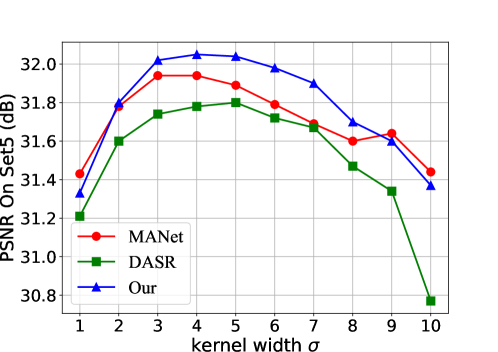
Performance Evaluation. Five benchmark datasets are used for evaluation: Set5 (Bevilacqua et al., 2012), Set14 (Zeyde et al., 2010), BSD100 (Martin et al., 2001), Urban100 (Huang et al., 2015), and DIV2KRK (Bell-Kligler et al., 2019). Followed by previous work (Liang et al., 2021; Luo et al., 2022), Set5, Set14, B100 and Urban100 are degraded by $9$ different kernels: for $\times 4$ kernels are sampled from $\sigma_{1},\sigma_{2}\in\{1,5,9\}$ and $\theta\in\{0,\frac{pi}{4}\}$; for $\times 2$ and $\times 3$, the kernels set varies to $\sigma_{1},\sigma_{2}\in\{1,3,5\}$ and $\sigma_{1},\sigma_{2}\in\{1,4,7\}$, respectively. The proposed model is evaluated by PSNR and SSIM on the Y channel of the SR in YCbCr space.

5.2. Comparison with State-of-the-Art Methods

We conduct experiments on degradations with anisotropic Gaussian kernels and noise. We compare CDSR with baseline models and existing blind SR models. The results are shown in Table 2 and Fig. 4. For fair comparisons, we retrained some of the methods under the same experimental setting. As shown in Table 2, the proposed CDSR outperforms the existing UDP models (e.g., $\times 2$ 0.8 dB better than DASR) and achieves competitive performance on PSNR and SSIM when compared with the SKP methods (MANet). Although IKC and SRSVD struggle to estimate the accurate kernel prior by introducing the iteration kernel refinement and the adversarial network, respectively, they achieve poor performance when compared to MANet. In particular, MANet achieves the dominant results among the SKP-based methods. By restricting the receptive field within a moderate range, MANet can capture the locality of degradation features without distributing.

However, these approaches occupy a large computational cost due to the iteration (IKC) and the full-size kernel maps (MANet). Moreover, the SKP methods only consider the blur kernel, therefore, these methods suffer from severe performance drop when degradation is composed of multiple degradations (i.e., noise). On the contrary, UDP methods are not limited to learning the kernel and attempting to represent the degradation. KernelGAN gets the worst performance compared with other UDP methods. The implicit kernel prediction fails to capture accurate information when applied in severe degradation. HAN employs the attention mechanism to extract the refinement feature in the SR network, the degradation prior is ignored in this method resulting in poor performance. DIP leverages the network prior to generate the SR images and largely improves the results. However, DIP suffers from multiple degradations and fails to produce a suitable prior. DASR employs a discriminative degradation encoder by unsupervised contrastive learning and largely improves the performance. However, the domain gap between degradation space and textual space limits the results thus performing inferior to our method. It is worth noting that our method achieves superior performance compared with other models on multiple degradations (i.e., $\times 4$ with noise level $15$).

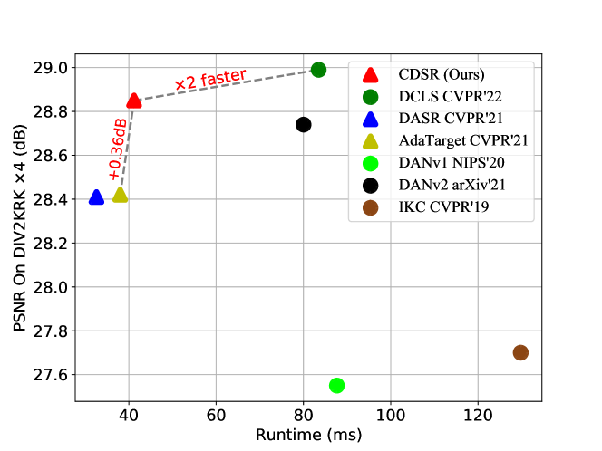
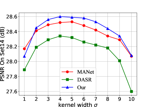
In addition, we retrain our model with the same experimental setting as previous methods on DIV2KRK (Bell-Kligler et al., 2019). The quantitative comparisons are shown in Fig. 5. It can be found that our proposed method can significantly outperform existing UDP methods and even shows the competitive results compared with the SKP methods. As an improved version of IKC, DAN has achieved remarkable performance using the iteration kernel refinement. In addition, DCLS largely improves the results by accurate estimation of kernel information. CDSR achieves the second-best of all the methods including SKP and UDP methods by taking 13.23 M while DCLS takes 19.05 M parameter’s amount. For SKP methods, CDSR is almost $2\times$ faster than DCLS (Test on a single V100) and achieves the competitive results compared with it. For UDP methods, CDSR outperforms the AdaTarget and the DASR by 0.36 dB on PSNR with similar computational cost. To show the variable trend with the change of $\sigma$ we also provide the various curves on Set5 and Set14, as shown in Fig. 6.

Figure 6. The PSNR curves on Set5 (left) and Set14 (right) of scale factor 4. The kernel width $\sigma_{1}=\sigma_{2}=[1:10:1]$.

	Bicubic	Model 2	Model 3
urban 67	Model 4	Model 5	Model 1
	15.81 dB	21.33 dB	22.97 dB
	22.24 dB	22.57 dB	23.21 dB

Figure 7. Different Visualized SR results ($\times 2$ ) for ablation study models on Urban100 Img 67.

5.3. Ablation Study

We conduct ablation studies to validate the effect of each component in our proposed method. The quantity results are shown in Table 3, and the quality visualizations are shown in Fig. 7. All the experiments are conducted on the scale factor of $\times 2$ setting.

Effect of Patch-wise Subnet. The patch-wise subnet in LPE is designed to extract the content information. Based on the content information, we can close the domain gap between the degradation embedding space and the texture space used in the SR network. To demonstrate its effect, we discard the patch-wise subnet and only apply the pixel-wise sub-net to extract the embedding. In addition, other components are maintained. Shown in Table 3 ”Model 4”, the performance significantly drops from $29.57$ to $29.16$.

Effect of Pixel-wise Subnet. We also test LPE without the pixel-wise subnet, denoted as Model 5. From the quantity results, we can find that pixel-wise subnet has a moderate effect. In other words, models with patch-wise subnet can preserve mainly SR capability. A reasonable explanation is the $\bm{E_{p}}$ is able to produce a promising embedding and $\bm{E_{l}}$ serves as the supplementary feature. This is also coherent with results in Table 1: the model which only focuses on local degradation features is inferior to that on content features.

Effect of DQA Module. In order to adaptively fuse the embedding prior to the SR network, the DQA module is proposed to reduce the domain gap. To study the effect of DQA, we conduct the experiment without it, which is denoted as Model 3. The self-attention mechanism applied in DQA can leverage the content cue to query the suitable embedding features, therefore there are fewer artifacts in the produced SR results. As shown in Fig. 7, the output of Model 4 suffers from the ghost artifacts, which are caused by the inconsistency of degradation embedding and SR feature.

Moreover, to demonstrate the effect of DQA, we compare this module with other fusion modules, as shown in Table 5. We first test the AdaIN approach. Specifically, instead of using Eq. 3, the embedding $\bm{E_{a}}$ is fed to MLP layers to produce the scale $\beta_{a}\in\mathbb{R}^{C\times 1}$ and the bias $\gamma_{a}\in\mathbb{R}^{C\times 1}$. The $\beta_{a}$ and $\gamma_{a}$ are used to refine the input features $\bm{F}_{i}$ by $\bm{\tilde{F}_{i}}=\beta_{a}*\bm{F}_{i}+\gamma_{a}$, where the $\beta_{a}$ and $\gamma_{a}$ are expanded along the spatial dimension. In addition, we also compared DQA with the standard dynamic convolution layer, shown in Table 5.

Effect of Codebook. Intuitively, an unconstrained embedding space prefers to preserve the redundant information. To enhance the robustness of LPE, the codebook is used to constrict the basis of embedding space. We conduct the experiment without the codebook in LPE denoted as ”Model 2”. As demonstrated in Table 3 and Fig. 7, the codebook can boost the performance of SR results.

5.4. Further Analysis

Our proposed method employs a prevalent framework of blind SR, which can be summered as two steps: (1) Degradation feature extraction; (2) embedding prior fusion in the non-blind SR network. Therefore, the encoder and non-blind SR network are more likely to have a win-win cooperation. CDSR takes the content information as the cue to connect them and achieve superior results. The experiments are conducted on the scale factor of $\times 2$ setting.

Is Content-aware Important? DASR employs a naive encoder and estimates the degradation-aware embedding by contrastive learning, and the content information is learned implicitly, as shown in Table 4. We replace the encoder of DASR Edasr by the patch-wise subnet LPEP to show the effect of content information (average increase of $0.33$ dB). Besides, we replace LPE with Edasr to validate the effect of LPE. Compared with DASR, the SR network with DQA can improve the output quality but is still inferior to our result. The reason may be Edasr introduces the perturbation to the SR network, and destroy the cooperative relationship between LPE and DQA.

Is Local-aware Enough? For the elaborate design of channel-wise relation extraction in MANet, it achieves more promising results than Edasr because of the moderate receptive field. In order to study whether the performance is improved by the channel-wise mutual computation or the local receptive field, we conduct the experiments with the LPEL (i.e., MANet vs LPEL). LPEL only applies several convolution layers while MANet suffers from huge computational costs. The result shows that simply fixing the small receptive field does not share the competitive performance of MANet, but is better than Edasr, especially in the tough case (e.g., $29.16$ dB vs $28.96$ dB in Urban100). It is worth noting that the performance can be significantly improved when combining the LPEL and LPEP.

Computation Cost and Parameters. For the computational cost, we study the capability of our model with different numbers of blocks in the SR network. The inference Giga Floating-point Operations Per Second (GFlops) and the total amount of parameters are used to evaluate the computational cost. As shown in Table 6, DASR takes fewer GFlops and parameters to achieve moderate performance. To prove the superiority is caused by the effective design rather than the computation increasing, we shrink our model by modifying the numbers of blocks used in our SR network. When the computational cost is restricted to the same level, our proposed method is still able to outperform DASR. In addition, the model utilizes similar computational cost to MANet and can achieve competitive performance when compared with the SOTA SKP methods.

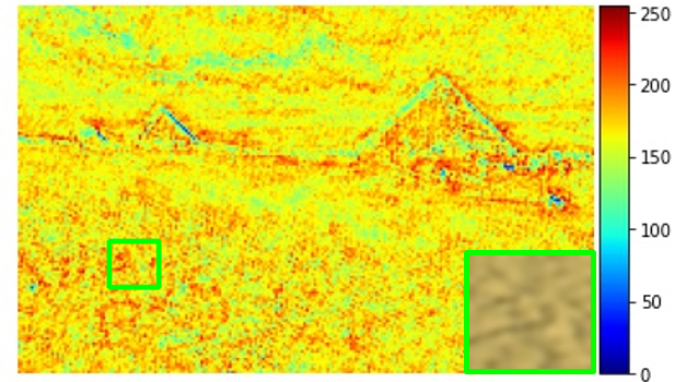
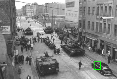
Performance on Real Degradation. To further demonstrate the effectiveness of our method, following  (Wang et al., 2021), we test our model on the real images. Visualization results are shown in Fig. 8, compared with the SOTA methods, CDSR can provide more clear results, especially for the edge.

Table 6. Performance and complexity for $48$$\times$$48$ image.

Model	Gflops (G)	Param. (M)	BSD100
DASR	5.97	5.82	30.46/0.8507
MANet	21.39	9.9	30.97/0.8651
1-4[3pt/2.5pt] Ours (Blks=2)	4.93	5.24	30.72/0.8600
Ours (Blks=5)	10.47	8.24	30.86/0.8605
Ours (Blks=10)	19.72	13.23	31.02/0.8643

	DASR	HAN
real image	MANet	Ours

Figure 8. Visual results of different methods on real image for $\times 4$ SR. Ours provides more clear results.

6. Conclusion

In this paper, we study the problem of what kind of embedding is needed for blind SR. By deriving the truth that content information can serve as the cue for SR feature, we propose CDSR that jointly learns the content and degradation aware embedding feature for blind SR. Specifically, the LPE is exploited to produce the degradation meanwhile preserving the content information. Then, the proposed DQA module can leverage the content information to adaptively query the degradation information. Furthermore, we introduce the CSC to limit the basis of feature space and achieve end-to-end training. Extensive experiments demonstrate that the proposed CDSR is able to achieve competitive results.

Here we provide more details for the proposed CDSR. We first give the architecture of the LPE and the DQA based non-blind SR model. Then we provide more experiments results for CDSR. Last, we report more quantity and quality results of CDSR.

Appendix A Training Details of CDSR

The CDSR is trained end-to-end, different from the DASR (Wang et al., 2021) which requires to pretrain the encoder for 100 epoch, CDSR jointly train the encoder and non-blind SR in order to product more adaptive feature. Besides, different from the MANet (Liang et al., 2021) which employs complex multi-training stages, CDSR is easy to be trained. The Adam optimizer with the momentum of $\beta_{1}=0.9$ , $\beta_{2}=0.999$ is adopted to train our network with the learning rate being initially set to $1e-4$. the learning rate will decay by half after every $125$ epochs by the multi-step decreasing strategy. The training process takes $500$ epoch. The training time is about 2 days on a Tesla V100 GPU.

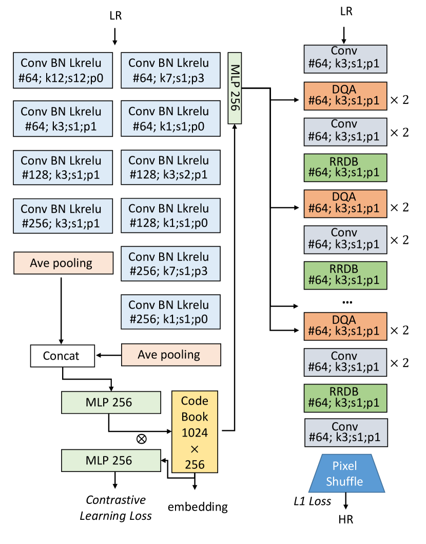
A.1. Framework

The framework details of CDSR is shown in Fig. 9. CDSR is composed of two parts: (1) degradation prior encoder; (2) DQA based non-blind SR network.

Figure 9. The framework of proposed CDSR. The basic block is composed by convolutional layer, batch normalization layer, leaky relu. ‘#’ denotes the number of filters, ‘k’ denotes the kernel size and ‘p’ denotes the padding size. The $otimes$ denotes the matrix multiplication.

Table 7. Quantitative comparison on DIV2KRK. The best result is marked in red. The ‘SK’ denotes whether correspond method belongs to SKP or UDP.

Method	SK	DIV2KRK
		$\times 2$	$\times 4$
IKC (Gu et al., 2019)	✓	-	27.70/0.7668
DANv1 (Huang et al., 2020)	✓	32.56/0.8997	27.55/0.7582
DANv2 (Luo et al., 2021)	✓	32.58/0.9048	28.74/0.7893
KOALAnet (Kim et al., 2021)	✓	31.89/0.8852	27.77/0.7637
DCLS (Luo et al., 2022)	✓	32.75/0.9094	28.99/0.7946
Ours-SKP	✓	32.76/0.9050	28.87/0.7923
1-4[3pt/2.5pt] DBPN + Correction	✕	30.38/0.8717	26.79/0.7426
KernelGAN + ZSSR	✕	30.36/0.8669	26.81/0.7316
AdaTarget	✕	-	28.42/0.7854
DASR	✕	32.24/0.8960	28.41/0.7813
Ours	✕	32.68/0.9039	28.85/0.7901

Appendix B More Experiments

B.1. More details of DIV2KRK.

Here we provide more quality comparison results for SOTA methods on DIV2KRK test set. CDSR achieves the second-best of all the methods including SKP and UDP methods by taking 13.23 M while DCLS takes 19.05 M parameter’s amount. We also experiment CDSR in a SKP manner (Ours-SKP), specifically, we add a MLP with 5 layers taking the embedding as input and predict the kernel value. Specifically, the mean absolute error (MAE) is used as the loss function to measure the difference between estimated kernels and ground-truth kernels. Then the embedding are used in the DQA based non-blind SR. The results are shown in Table 7.

B.2. More details for experiments

In supplementary we report the whole results for the models in our ablation study on Set5, Set14, BSD100, and Uraban100 test sets (Table 8). In addition, we also provide the whole results for the models in Sec 5.4 in Table 9 and Table 10.

Table 8. More details of ablation study for $\times 2$ SR .

Model	LPEL	LPEP	DQA	CSC	Set5	Set14	BSD100	Urban100
Model 1	✓	✓	✓	✓	36.17/0.9428	32.14/0.8841	31.02/0.8643	29.57/0.8851
Model 2	✓	✓	✓	✕	36.01/0.9416	32.03/0.8811	30.90/0.8611	29.36/0.8828
Model 3	✓	✓	✕	✓	36.04/0.9427	31.71/0.8842	30.85/0.8678	29.32/0.8889
Model 4	✓	✕	✓	✓	35.84/0.9400	31.86/0.8787	30.80/0.8594	29.16/0.8775
Model 5	✕	✓	✓	✓	35.98/0.9414	32.07/0.8819	30.89/0.8609	29.44/0.8827

Table 9. More details of further analysis for $\times 2$ SR.

Model	Set5	Set14	BSD100	Urban100
SRdasr + Edasr	35.30/0.9360	31.30/0.8683	30.46/0.8507	28.66/0.8654
SRdasr + LPEP	35.55/0.9290	31.65/0.8796	30.73/0.8603	29.10/0.8796
SROurs + Edasr	35.90/0.9406	31.77/0.8777	30.81/0.8590	28.96/0.8738
SROurs + Emanet	35.94/0.9409	32.08/0.8825	30.94/0.8624	29.44/0.8829
SROurs+LPEL	35.84/0.9400	31.86/0.8787	30.80/0.8594	29.16/0.8775
SROurs+LPE	36.17/0.9428	32.14/0.8841	31.02/0.8643	29.57/0.8851

Table 10. More details of computational cost for $\times 2$ SR.

Model	Gflops (G)	Param. (M)	Set5	Set14	BSD100	Urban100
DASR	5.97	5.82	35.30/0.9360	31.30/0.8683	30.46/0.8507	28.66/0.8654
MANet	21.39	9.9	35.98/0.9420	31.95/0.8845	30.97/0.8651	29.61/0.8880
1-7[3pt/2.5pt] Ours (Blks=2)	4.93	5.24	35.60/0.9401	31.69/0.8812	30.72/0.8600	28.91/0.8737
Ours (Blks=5)	10.47	8.24	35.92/0.9407	31.90/0.8809	30.86/0.8605	29.18/0.8784
Ours (Blks=10)	19.72	13.23	36.17/0.9428	32.14/0.8841	31.02/0.8643	29.57/0.8851

Table 11. The effect of codebook with different length for $\times 2$ SR.

CodeBook Length	Set5	Set14	BSD100	Urban100
1024	36.17/0.9428	32.14/0.8841	31.02/0.8643	29.57/0.8851
2048	36.11/0.9424	32.14/0.8844	30.96/0.8631	29.59/0.8865

Table 12. The impact of pretraining the encoder for $\times 2$ SR.

Pretrain Encoder	Set5	Set14	BSD100	Urban100
100 epcoh	36.08/0.9417	32.05/0.8822	30.91/0.8611	29.44/0.8826
0 epoch	36.17/0.9428	32.14/0.8841	31.02/0.8643	29.57/0.8851

B.3. About the length of codebook.

We also conduct the experiments of different length of codebook. As shown in Table 11, the larger codebook can not produce the competitive results with that of original length. The Codebook-based Space Compress module (CSC) is designed to limit the basis of feature space, thus reducing redundancy and mitigating the domain gap between degradation and content spaces. Once enlarging the codebook, the redundancy can not be suppressed and the larger codebook will reduce the constraint of space basis.

B.4. Pretrained encoder.

Both DASR and MANet employ a complex training strategies to train their models: pretrain the encoders (DASR); pretrain the kernel predictor (MANet). However, CDSR is trained end-to-end and we find that the pretrain encoder will drops the performance of CDSR. We conduct the experiment that firstly pretrain 100 epoch of the encoder and then train the encoder and SR network together, the results is shown in Table 12. An explanation is that, the joint training let the encoder to produce a more adaptive embedding and easy to learn the content and degradation aware embedding.

References

- (1)
- Abu Hussein et al. (2020) Shady Abu Hussein, Tom Tirer, and Raja Giryes. 2020. Correction Filter for Single Image Super-Resolution: Robustifying Off-the-Shelf Deep Super-Resolvers. IEEE Conf. Comput. Vis. Pattern Recog. (2020).
- Agustsson and Timofte (2017) Eirikur Agustsson and Radu Timofte. 2017. NTIRE 2017 Challenge on Single Image Super-Resolution: Dataset and Study. In IEEE Conf. Comput. Vis. Pattern Recog. Worksh.
- Bell-Kligler et al. (2019) Sefi Bell-Kligler, Assaf Shocher, and Michal Irani. 2019. Blind super-resolution kernel estimation using an internal-gan. Adv. Neural Inform. Process. Syst. 32 (2019).
- Bevilacqua et al. (2012) Marco Bevilacqua, Aline Roumy, Christine Guillemot, and Marie Line Alberi-Morel. 2012. Low-complexity single-image super-resolution based on nonnegative neighbor embedding. (2012).
- Chen et al. (2020) Ting Chen, Simon Kornblith, Mohammad Norouzi, and Geoffrey Hinton. 2020. A simple framework for contrastive learning of visual representations. PMLR, 1597–1607.
- Cornillere et al. (2019) Victor Cornillere, Abdelaziz Djelouah, Wang Yifan, Olga Sorkine-Hornung, and Christopher Schroers. 2019. Blind image super-resolution with spatially variant degradations. ACM Transactions on Graphics (TOG) 38, 6 (2019), 1–13.
- Dai et al. (2019) Tao Dai, Jianrui Cai, Yongbing Zhang, Shu-Tao Xia, and Lei Zhang. 2019. Second-order attention network for single image super-resolution. In IEEE Conf. Comput. Vis. Pattern Recog. 11065–11074.
- Dong et al. (2014) Chao Dong, Chen Change Loy, Kaiming He, and Xiaoou Tang. 2014. Learning a deep convolutional network for image super-resolution. In Eur. Conf. Comput. Vis. Springer, 184–199.
- Dong et al. (2016) Chao Dong, Chen Change Loy, and Xiaoou Tang. 2016. Accelerating the super-resolution convolutional neural network. In Eur. Conf. Comput. Vis. Springer, 391–407.
- Dosovitskiy et al. (2021) Alexey Dosovitskiy, Lucas Beyer, Alexander Kolesnikov, Dirk Weissenborn, Xiaohua Zhai, Thomas Unterthiner, Mostafa Dehghani, Matthias Minderer, Georg Heigold, Sylvain Gelly, Jakob Uszkoreit, and Neil Houlsby. 2021. An Image is Worth 16x16 Words: Transformers for Image Recognition at Scale. In Int. Conf. Learn. Represent.
- Gu et al. (2019) Jinjin Gu, Hannan Lu, Wangmeng Zuo, and Chao Dong. 2019. Blind super-resolution with iterative kernel correction. In IEEE Conf. Comput. Vis. Pattern Recog. 1604–1613.
- Haris et al. (2018) Muhammad Haris, Gregory Shakhnarovich, and Norimichi Ukita. 2018. Deep back-projection networks for super-resolution. In IEEE Conf. Comput. Vis. Pattern Recog. 1664–1673.
- He et al. (2020) Kaiming He, Haoqi Fan, Yuxin Wu, Saining Xie, and Ross Girshick. 2020. Momentum contrast for unsupervised visual representation learning. In IEEE Conf. Comput. Vis. Pattern Recog. 9729–9738.
- Hinton and Roweis (2002) Geoffrey E Hinton and Sam Roweis. 2002. Stochastic neighbor embedding. Adv. Neural Inform. Process. Syst. 15 (2002).
- Huang et al. (2015) Jia-Bin Huang, Abhishek Singh, and Narendra Ahuja. 2015. Single image super-resolution from transformed self-exemplars. In IEEE Conf. Comput. Vis. Pattern Recog. 5197–5206.
- Huang and Belongie (2017) Xun Huang and Serge Belongie. 2017. Arbitrary style transfer in real-time with adaptive instance normalization. In Int. Conf. Comput. Vis. 1501–1510.
- Huang et al. (2020) Yan Huang, Shang Li, Liang Wang, Tieniu Tan, et al. 2020. Unfolding the alternating optimization for blind super resolution. Adv. Neural Inform. Process. Syst. 33 (2020), 5632–5643.
- Hussein et al. (2020) Shady Abu Hussein, Tom Tirer, and Raja Giryes. 2020. Correction filter for single image super-resolution: Robustifying off-the-shelf deep super-resolvers. In Proceedings of the IEEE/CVF Conference on Computer Vision and Pattern Recognition. 1428–1437.
- Jia et al. (2016) Xu Jia, Bert De Brabandere, Tinne Tuytelaars, and Luc V Gool. 2016. Dynamic filter networks. Adv. Neural Inform. Process. Syst. 29 (2016).
- Johnson et al. (2016) Justin Johnson, Alexandre Alahi, and Li Fei-Fei. 2016. Perceptual losses for real-time style transfer and super-resolution. In Eur. Conf. Comput. Vis. Springer, 694–711.
- Kim et al. (2016a) Jiwon Kim, Jung Kwon Lee, and Kyoung Mu Lee. 2016a. Accurate image super-resolution using very deep convolutional networks. In IEEE Conf. Comput. Vis. Pattern Recog. 1646–1654.
- Kim et al. (2016b) Jiwon Kim, Jung Kwon Lee, and Kyoung Mu Lee. 2016b. Deeply-recursive convolutional network for image super-resolution. In IEEE Conf. Comput. Vis. Pattern Recog. 1637–1645.
- Kim et al. (2021) Soo Ye Kim, Hyeonjun Sim, and Munchurl Kim. 2021. KOALAnet: Blind Super-Resolution using Kernel-Oriented Adaptive Local Adjustment. In IEEE Conf. Comput. Vis. Pattern Recog. 10611–10620.
- Kumar et al. (2022) Manoj Kumar, Neil Houlsby, Nal Kalchbrenner, and Ekin D Cubuk. 2022. On the surprising tradeoff between ImageNet accuracy and perceptual similarity. arXiv preprint arXiv:2203.04946 (2022).
- Ledig et al. (2017) Christian Ledig, Lucas Theis, Ferenc Huszár, Jose Caballero, Andrew Cunningham, Alejandro Acosta, Andrew Aitken, Alykhan Tejani, Johannes Totz, Zehan Wang, et al. 2017. Photo-realistic single image super-resolution using a generative adversarial network. In IEEE Conf. Comput. Vis. Pattern Recog. 4681–4690.
- Liang et al. (2021) Jingyun Liang, Guolei Sun, Kai Zhang, Luc Van Gool, and Radu Timofte. 2021. Mutual affine network for spatially variant kernel estimation in blind image super-resolution. In Int. Conf. Comput. Vis. 4096–4105.
- Lugmayr et al. (2020) Andreas Lugmayr, Martin Danelljan, Luc Van Gool, and Radu Timofte. 2020. Srflow: Learning the super-resolution space with normalizing flow. In Eur. Conf. Comput. Vis. Springer, 715–732.
- Luo et al. (2022) Ziwei Luo, Haibin Huang, Lei Yu, Youwei Li, Haoqiang Fan, and Shuaicheng Liu. 2022. Deep Constrained Least Squares for Blind Image Super-Resolution. In IEEE Conf. Comput. Vis. Pattern Recog.
- Luo et al. (2021) Zhengxiong Luo, Yan Huang, Shang Li, Liang Wang, and Tieniu Tan. 2021. End-to-end Alternating Optimization for Blind Super Resolution. arXiv:2105.06878 [cs.CV]
- Martin et al. (2001) David Martin, Charless Fowlkes, Doron Tal, and Jitendra Malik. 2001. A database of human segmented natural images and its application to evaluating segmentation algorithms and measuring ecological statistics. In Int. Conf. Comput. Vis., Vol. 2. IEEE, 416–423.
- Niu et al. (2020) Ben Niu, Weilei Wen, Wenqi Ren, Xiangde Zhang, Lianping Yang, Shuzhen Wang, Kaihao Zhang, Xiaochun Cao, and Haifeng Shen. 2020. Single image super-resolution via a holistic attention network. In European conference on computer vision. Springer, 191–207.
- Noroozi et al. (2017) Mehdi Noroozi, Hamed Pirsiavash, and Paolo Favaro. 2017. Representation learning by learning to count. In Int. Conf. Comput. Vis. 5898–5906.
- Singh et al. (2014) Abhishek Singh, Fatih Porikli, and Narendra Ahuja. 2014. Super-resolving noisy images. In IEEE Conf. Comput. Vis. Pattern Recog. 2846–2853.
- Soh et al. (2020) Jae Woong Soh, Sunwoo Cho, and Nam Ik Cho. 2020. Meta-transfer learning for zero-shot super-resolution. In IEEE Conf. Comput. Vis. Pattern Recog. 3516–3525.
- Tai et al. (2017a) Ying Tai, Jian Yang, and Xiaoming Liu. 2017a. Image Super-Resolution via Deep Recursive Residual Network. In Proceedings of the IEEE Conference on Computer Vision and Pattern Recognition.
- Tai et al. (2017b) Ying Tai, Jian Yang, Xiaoming Liu, and Chunyan Xu. 2017b. Memnet: A persistent memory network for image restoration. In Proceedings of the IEEE international conference on computer vision. 4539–4547.
- Tao et al. (2021) Guangpin Tao, Xiaozhong Ji, Wenzhuo Wang, Shuo Chen, Chuming Lin, Yun Cao, Tong Lu, Donghao Luo, and Ying Tai. 2021. Spectrum-to-Kernel Translation for Accurate Blind Image Super-Resolution. Adv. Neural Inform. Process. Syst. 34 (2021).
- Tian et al. (2020) Yonglong Tian, Dilip Krishnan, and Phillip Isola. 2020. Contrastive multiview coding. In Eur. Conf. Comput. Vis. Springer, 776–794.
- Timofte et al. (2017) Radu Timofte, Eirikur Agustsson, Luc Van Gool, Ming-Hsuan Yang, and Lei Zhang. 2017. Ntire 2017 challenge on single image super-resolution: Methods and results. In IEEE Conf. Comput. Vis. Pattern Recog. Worksh. 114–125.
- Trockman and Kolter (2022) Asher Trockman and J Zico Kolter. 2022. Patches Are All You Need? arXiv preprint arXiv:2201.09792 (2022).
- Ulyanov et al. (2018) Dmitry Ulyanov, Andrea Vedaldi, and Victor Lempitsky. 2018. Deep image prior. In Proceedings of the IEEE conference on computer vision and pattern recognition. 9446–9454.
- Wang et al. (2021) Longguang Wang, Yingqian Wang, Xiaoyu Dong, Qingyu Xu, Jungang Yang, Wei An, and Yulan Guo. 2021. Unsupervised Degradation Representation Learning for Blind Super-Resolution. In IEEE Conf. Comput. Vis. Pattern Recog.
- Wang et al. (2018) Xintao Wang, Ke Yu, Chao Dong, and Chen Change Loy. 2018. Recovering realistic texture in image super-resolution by deep spatial feature transform. In IEEE Conf. Comput. Vis. Pattern Recog. 606–615.
- Xu et al. (2020) Yu-Syuan Xu, Shou-Yao Roy Tseng, Yu Tseng, Hsien-Kai Kuo, and Yi-Min Tsai. 2020. Unified dynamic convolutional network for super-resolution with variational degradations. In IEEE Conf. Comput. Vis. Pattern Recog. 12496–12505.
- Zeyde et al. (2010) Roman Zeyde, Michael Elad, and Matan Protter. 2010. On single image scale-up using sparse-representations. In International conference on curves and surfaces. Springer, 711–730.
- Zhang et al. (2021b) Jiahui Zhang, Shijian Lu, Fangneng Zhan, and Yingchen Yu. 2021b. Blind image super-resolution via contrastive representation learning. arXiv preprint arXiv:2107.00708 (2021).
- Zhang et al. (2020) Kai Zhang, Luc Van Gool, and Radu Timofte. 2020. Deep unfolding network for image super-resolution. In IEEE Conf. Comput. Vis. Pattern Recog. 3217–3226.
- Zhang et al. (2021a) Kai Zhang, Jingyun Liang, Luc Van Gool, and Radu Timofte. 2021a. Designing a practical degradation model for deep blind image super-resolution. In IEEE Conf. Comput. Vis. Pattern Recog. 4791–4800.
- Zhang et al. (2018d) Kai Zhang, Wangmeng Zuo, and Lei Zhang. 2018d. Learning a single convolutional super-resolution network for multiple degradations. In IEEE Conf. Comput. Vis. Pattern Recog. 3262–3271.
- Zhang et al. (2018a) Richard Zhang, Phillip Isola, Alexei A Efros, Eli Shechtman, and Oliver Wang. 2018a. The unreasonable effectiveness of deep features as a perceptual metric. In IEEE Conf. Comput. Vis. Pattern Recog. 586–595.
- Zhang et al. (2018b) Yulun Zhang, Kunpeng Li, Kai Li, Lichen Wang, Bineng Zhong, and Yun Fu. 2018b. Image super-resolution using very deep residual channel attention networks. In Eur. Conf. Comput. Vis. 286–301.
- Zhang et al. (2018c) Yulun Zhang, Kunpeng Li, Kai Li, Lichen Wang, Bineng Zhong, and Yun Fu. 2018c. Image super-resolution using very deep residual channel attention networks. In Eur. Conf. Comput. Vis. 286–301.