Eco-Evolutionary Dynamics of Bimatrix Games

Longmei Shu Feng Fu
Abstract

Feedbacks between strategies and the environment are common in social-ecological, evolutionary-ecological, and even psychological-economic systems. Utilizing common resources is always a dilemma for community members, like tragedy of the commons. Here we consider replicator dynamics with feedback-evolving games, where the payoffs switch between two different matrices. Although each payoff matrix on its own represents an environment where cooperators and defectors can’t coexist stably, we show that it’s possible to design appropriate switching control laws and achieve persistent oscillations of strategy abundance. This result should help guide the widespread problem of population state control in microbial experiments and other social problems with eco-evolutionary feedback loops.

keywords:
asymmetrical games , changing environment , evolutionary game theory, switching control
journal: journal
\affiliation

[inst1]organization=Department of Mathematics,addressline=Dartmouth College, city=Hanover, postcode=03755, state=NH, country=USA

\affiliation

[inst2]organization=Department of Biomedical Data Science,addressline=Geisel School of Medicine at Dartmouth, city=Lebanon, postcode=03756, state=NH, country=USA

1 Introduction

Game theory is based on the principle that individuals make rational decisions regarding their choice of actions given suitable incentives [1]. In practice, the incentives are represented as strategy-dependent payoffs. Evolutionary game theory extends game-theoretic principles to model dynamic changes in the frequency of strategies [2, 3]. Replicator dynamics is one commonly used framework for such models [4]. In replicator dynamics, the frequency of strategists changes over time as a function of the social makeup of the community. The frequency of a strategy increases when the fitness of those who adopt it is greater than the average fitness of the population.

But individual actions do not only modify the social makeup, they very often modify the environment as well [5]. The strategies that individuals employ impact the environment through time, and the state of the environment in turn influences the payoffs of the game. This environment-dependent feedback occurs across scales from microbes [6, 7, 8, 9] to humans [10, 11, 12, 13, 14, 15] in public goods game and the tragedy of the commons [16]. The tragedy of the commons is a fundamental problem that is intensively studied [17, 18, 19, 20]. A well-known example is the danger of overfishing. Fishermen are motivated to catch the maximum amount of fish because restraint could only work if all others were behaving similarly. Otherwise, fish are driven to extinction which is the worst scenario for everyone. Similarly, in overgrazing of common pasture lands, an individual’s short-term benefit seems to be in conflict with the long-term interest of a larger population. The common feature of these cases is human activity influences the actual state of resources which has a negative feedback for not only those who degrade the environment but also for the whole community.

The feedback loop between the environment and individual behavioral strategies also appears in microbial populations [21], including microbes, bacteria, and viruses. Among microbes, feedback may arise due to fixation of inorganic nutrients given depleted organic nutrient availability, the production of extracellular nutrient-scavenging enzymes like siderophores or enzymes like invertase that hydrolyze diffusible products, and the release of extracellular antibiotic compounds. The incentive for public goods production changes as the production influences the environmental state.

Such joint influence occurs in human societies [22], for example, when individuals decide to vaccinate or not [23]. Decisions not to vaccinate have been linked most recently to outbreaks of otherwise-preventable childhood infectious diseases in northern California. These outbreaks modify the subsequent incentives for vaccination. Such coupled feedback also arises in public goods dilemmas involving water [24] or other resource use such as antibiotic use [25]. In a period of replete resources, there is less incentive for restraint. However, overuse in times of replete resource availability can lead to depletion of the resource and changes in incentives.

A new framework of replicator dynamics with feedback-evolving games has been proposed [10] to characterize the phenomenon that the environment and individual behavior co-evolve in many social-ecological and psychological-economic systems [26]. The environmental feedback can result in oscillating dynamics for both the environment quality and strategy states, for example, multiple waves of infections as seen in the COVID-19 pandemic [27]. This unified approach to analyze and understand feedback-evolving games is called eco-evolutionary game theory. It denotes the coupled evolution of strategies and the environment. The cumulative feedback of decisions can subsequently alter environment-dependent incentives, thereby leading to new dynamical phenomena and new challenges for control.

Utilizing common resources always imposes a dilemma for community members. While cooperators restrain themselves and help maintain the proper state of resources, defectors demand more than their supposed share for a higher payoff. The nature of the feedback and the rate of ecological changes can relax or aggravate social dilemmas and promote persistent periodic oscillations of strategy abundance and environmental quality. To alleviate the tragedy of the commons, questions that inspire our present work include: how to manage and conserve public resources, which processes drive human cooperation, and how institutions, norms and other feedback mechanisms can be used to reinforce positive behaviors.

Strategies and the environment are coupled. In human societies the institutions structuring social interactions can be seen as part of the environment that co-evolve with strategic behaviors. Many problems need to be solved like pollution control and climate change mitigation, and the proper management of food webs, soil weathering, and earth system processes. The psychology of decision-making, species interaction and climate change action.

In this paper we show some simple examples where the original system has unstable equilibria under two distinct environments, and we can trap the system between the unstable equilibria to achieve a dynamic steady state for the system. We hope this can provide some intuition for policy making in social dilemmas. Controlled decision making is likely to be costly but will allow individuals to choose optimal behavior.

2 Model

Consider a two player asymmetrical game of normal form. Player 1 has the strategy set S={s1,s2}𝑆subscript𝑠1subscript𝑠2S=\{s_{1},s_{2}\}, and player 2 has the strategy set T={t1,t2}𝑇subscript𝑡1subscript𝑡2T=\{t_{1},t_{2}\}. When the pair of strategies (si,tj)subscript𝑠𝑖subscript𝑡𝑗(s_{i},t_{j}) is chosen, the payoff to player 1 is aij=u1(si,tj)subscript𝑎𝑖𝑗subscript𝑢1subscript𝑠𝑖subscript𝑡𝑗a_{ij}=u_{1}(s_{i},t_{j}) and the payoff to player 2 is bij=u2(si,tj)subscript𝑏𝑖𝑗subscript𝑢2subscript𝑠𝑖subscript𝑡𝑗b_{ij}=u_{2}(s_{i},t_{j}). Then the values of the payoff functions can be given by two matrices, respectively, for the two types of players 1 and 2,

A=[a11a12a21a22],B=[b11b12b21b22].formulae-sequence𝐴matrixsubscript𝑎11subscript𝑎12subscript𝑎21subscript𝑎22𝐵matrixsubscript𝑏11subscript𝑏12subscript𝑏21subscript𝑏22A=\begin{bmatrix}a_{11}&a_{12}\\ a_{21}&a_{22}\end{bmatrix},\quad B=\begin{bmatrix}b_{11}&b_{12}\\ b_{21}&b_{22}\end{bmatrix}.

We put these two matrices together in the following canonical way for a bimatrix game.

M=AB=[(a11,b11)(a12,b12)(a21,b21)(a22,b22)].𝑀direct-sum𝐴𝐵matrixsubscript𝑎11subscript𝑏11subscript𝑎12subscript𝑏12subscript𝑎21subscript𝑏21subscript𝑎22subscript𝑏22M=A\oplus B=\begin{bmatrix}(a_{11},b_{11})&(a_{12},b_{12})\\ (a_{21},b_{21})&(a_{22},b_{22})\end{bmatrix}.

Now we consider a bimatrix game where the payoff bimatrix is not constant and depends on the environment.

M(t)=[(a11(t),b11(t))(a12(t),b12(t))(a21(t),b21(t))(a22(t),b22(t))].𝑀𝑡matrixsubscript𝑎11𝑡subscript𝑏11𝑡subscript𝑎12𝑡subscript𝑏12𝑡subscript𝑎21𝑡subscript𝑏21𝑡subscript𝑎22𝑡subscript𝑏22𝑡M(t)=\begin{bmatrix}\left(a_{11}(t),b_{11}(t)\right)&\left(a_{12}(t),b_{12}(t)\right)\\ \left(a_{21}(t),b_{21}(t)\right)&\left(a_{22}(t),b_{22}(t)\right)\end{bmatrix}.

For simplicity, we start with the combination of two constant bimatrices,

M(t)=η(t)MI+(1η(t))MII,𝑀𝑡𝜂𝑡subscript𝑀𝐼1𝜂𝑡subscript𝑀𝐼𝐼\displaystyle M(t)=\eta(t)M_{I}+(1-\eta(t))M_{II},

where

MI=[(a11,b11)(a12,b12)(a21,b21)(a22,b22)],MII=[(a11,b11)(a12,b12)(a21,b21)(a22,b22)],formulae-sequencesubscript𝑀𝐼matrixsubscript𝑎11subscript𝑏11subscript𝑎12subscript𝑏12subscript𝑎21subscript𝑏21subscript𝑎22subscript𝑏22subscript𝑀𝐼𝐼matrixsuperscriptsubscript𝑎11superscriptsubscript𝑏11superscriptsubscript𝑎12superscriptsubscript𝑏12superscriptsubscript𝑎21superscriptsubscript𝑏21superscriptsubscript𝑎22superscriptsubscript𝑏22\displaystyle M_{I}=\begin{bmatrix}(a_{11},b_{11})&(a_{12},b_{12})\\ (a_{21},b_{21})&(a_{22},b_{22})\end{bmatrix},M_{II}=\begin{bmatrix}(a_{11}^{\prime},b_{11}^{\prime})&(a_{12}^{\prime},b_{12}^{\prime})\\ (a_{21}^{\prime},b_{21}^{\prime})&(a_{22}^{\prime},b_{22}^{\prime})\end{bmatrix},

and η(t)𝜂𝑡\eta(t) is the environment evolving indicator as the environment switches between two states I and II. There are many possibilities for the function η(t)𝜂𝑡\eta(t). One of them is the following periodic function.
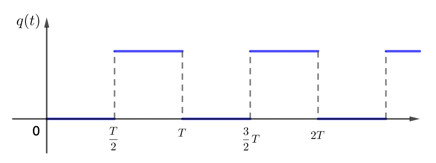
q(t)={0,kTt<kT+T/2,k=0,1,2,1,kT+T/2t<(k+1)T,k=0,1,2,𝑞𝑡cases0𝑘𝑇𝑡𝑘𝑇𝑇2𝑘0121𝑘𝑇𝑇2𝑡𝑘1𝑇𝑘012q(t)=\begin{cases}0,\qquad kT\leq t<kT+T/2,&k=0,1,2,\dots\\ 1,\qquad kT+T/2\leq t<(k+1)T,&k=0,1,2,\dots\end{cases}
Refer to caption
Figure 1: Periodic switching between two environments

Now we introduce mixed strategies in our game and assume X=(x1,x2)𝑋subscript𝑥1subscript𝑥2X=(x_{1},x_{2}), where x1subscript𝑥1x_{1} represents the probability of player 1 choosing strategy s1=lsubscript𝑠1𝑙s_{1}=l and x2subscript𝑥2x_{2} represents the probability of player 1 choosing strategy s2=rsubscript𝑠2𝑟s_{2}=r. We have

x1+x2=1.subscript𝑥1subscript𝑥21x_{1}+x_{2}=1.

Similarly we have Y=(y1,y2)𝑌subscript𝑦1subscript𝑦2Y=(y_{1},y_{2}) where y1,y2subscript𝑦1subscript𝑦2y_{1},y_{2} represent the probabilities of player 2 choosing strategies t1=Lsubscript𝑡1𝐿t_{1}=L and t2=Rsubscript𝑡2𝑅t_{2}=R. Then

y1+y2=1.subscript𝑦1subscript𝑦21y_{1}+y_{2}=1.

We note that identical notations and equations can be used to describe eco-evolutionary dynamics in subpopulations consisting of type 1 and type 2 players.

The payoff of player 1 when choosing strategy s1=lsubscript𝑠1𝑙s_{1}=l is

πl(X,Y)=a11(t)y1+a12(t)y2.subscript𝜋𝑙𝑋𝑌subscript𝑎11𝑡subscript𝑦1subscript𝑎12𝑡subscript𝑦2\displaystyle\pi_{l}(X,Y)=a_{11}(t)y_{1}+a_{12}(t)y_{2}.

The payoff of player 1 when choosing strategy s2=rsubscript𝑠2𝑟s_{2}=r is

πr(X,Y)=a21(t)y1+a22(t)y2.subscript𝜋𝑟𝑋𝑌subscript𝑎21𝑡subscript𝑦1subscript𝑎22𝑡subscript𝑦2\displaystyle\pi_{r}(X,Y)=a_{21}(t)y_{1}+a_{22}(t)y_{2}.

Let E(π)=x1πl+x2πr𝐸𝜋subscript𝑥1subscript𝜋𝑙subscript𝑥2subscript𝜋𝑟E(\pi)=x_{1}\pi_{l}+x_{2}\pi_{r} be the expected payoff for player 1. The replicator equation for x1subscript𝑥1x_{1} is

x˙1=x1(πlE(π))=x1(1x1)(πlπr).subscript˙𝑥1subscript𝑥1subscript𝜋𝑙𝐸𝜋subscript𝑥11subscript𝑥1subscript𝜋𝑙subscript𝜋𝑟\dot{x}_{1}=x_{1}(\pi_{l}-E(\pi))=x_{1}(1-x_{1})(\pi_{l}-\pi_{r}).

Plug in the values of πl,πrsubscript𝜋𝑙subscript𝜋𝑟\pi_{l},\pi_{r}, we get

x˙1=x1(1x1)[(a11(t)y1+a12(t)y2)(a21(t)y1+a22(t)y2)].subscript˙𝑥1subscript𝑥11subscript𝑥1delimited-[]subscript𝑎11𝑡subscript𝑦1subscript𝑎12𝑡subscript𝑦2subscript𝑎21𝑡subscript𝑦1subscript𝑎22𝑡subscript𝑦2\dot{x}_{1}=x_{1}(1-x_{1})[(a_{11}(t)y_{1}+a_{12}(t)y_{2})-(a_{21}(t)y_{1}+a_{22}(t)y_{2})]. (1)

And the replicator equation for x2subscript𝑥2x_{2} is

x˙2=x˙1subscript˙𝑥2subscript˙𝑥1\dot{x}_{2}=-\dot{x}_{1}

since x1+x2=1subscript𝑥1subscript𝑥21x_{1}+x_{2}=1.

Similarly we can write down the payoffs of strategies t1=Lsubscript𝑡1𝐿t_{1}=L and t2=Rsubscript𝑡2𝑅t_{2}=R.

πL(X,Y)=b11(t)x1+b21(t)x2,subscript𝜋𝐿𝑋𝑌subscript𝑏11𝑡subscript𝑥1subscript𝑏21𝑡subscript𝑥2\displaystyle\pi_{L}(X,Y)=b_{11}(t)x_{1}+b_{21}(t)x_{2},
πR(X,Y)=b12(t)x1+b22(t)x2.subscript𝜋𝑅𝑋𝑌subscript𝑏12𝑡subscript𝑥1subscript𝑏22𝑡subscript𝑥2\displaystyle\pi_{R}(X,Y)=b_{12}(t)x_{1}+b_{22}(t)x_{2}.

The replicator equations for y1subscript𝑦1y_{1} and y2subscript𝑦2y_{2} are

y˙1=y1(1y1)(πLπR),subscript˙𝑦1subscript𝑦11subscript𝑦1subscript𝜋𝐿subscript𝜋𝑅\displaystyle\dot{y}_{1}=y_{1}(1-y_{1})(\pi_{L}-\pi_{R}),
y˙2=y˙1.subscript˙𝑦2subscript˙𝑦1\displaystyle\dot{y}_{2}=-\dot{y}_{1}.

Plug in the values of πLsubscript𝜋𝐿\pi_{L} and πRsubscript𝜋𝑅\pi_{R} we get

y˙1=y1(1y1)[(b11(t)x1+b21(t)x2)(b12(t)x1+b22(t)x2)].subscript˙𝑦1subscript𝑦11subscript𝑦1delimited-[]subscript𝑏11𝑡subscript𝑥1subscript𝑏21𝑡subscript𝑥2subscript𝑏12𝑡subscript𝑥1subscript𝑏22𝑡subscript𝑥2\dot{y}_{1}=y_{1}(1-y_{1})[(b_{11}(t)x_{1}+b_{21}(t)x_{2})-(b_{12}(t)x_{1}+b_{22}(t)x_{2})]. (2)

Equations (1),(2) combined with

η(t)=q(t)𝜂𝑡𝑞𝑡\eta(t)=q(t) (3)

governs the dynamics of our system.

3 Simple One-Dimensional Model

Before we try to solve the general 2-player bimatrix game (ABT)𝐴superscript𝐵𝑇(A\neq B^{T}), let’s start with the simplified one dimensional model obtained from assuming A=BT𝐴superscript𝐵𝑇A=B^{T}.

In this case, we have a system governed by the replicator equation of the following form

x˙=x(1x)[a(t)xb(t)],0<x<1formulae-sequence˙𝑥𝑥1𝑥delimited-[]𝑎𝑡𝑥𝑏𝑡0𝑥1\dot{x}=x(1-x)[a(t)x-b(t)],\quad 0<x<1 (4)

where a(t)=a11(t)a12(t)a21(t)+a22(t)𝑎𝑡subscript𝑎11𝑡subscript𝑎12𝑡subscript𝑎21𝑡subscript𝑎22𝑡a(t)=a_{11}(t)-a_{12}(t)-a_{21}(t)+a_{22}(t), and b(t)=a22(t)a12(t)𝑏𝑡subscript𝑎22𝑡subscript𝑎12𝑡b(t)=a_{22}(t)-a_{12}(t).

Let a=b(t)/a(t)superscript𝑎𝑏𝑡𝑎𝑡a^{*}=b(t)/a(t). As one can see, this equation has three equilibrium points, 0,1,a01superscript𝑎0,1,a^{*}. For our purposes, we only consider cases where a(0,1)superscript𝑎01a^{*}\in(0,1) by assuming the existence of an interior equilibrium,.

Based on the signs of a(t)𝑎𝑡a(t) and b(t)𝑏𝑡b(t), we have two possible situations for the phase line of the system.

Refer to caption
Figure 2: phase line of 1 dimensional replicator equation

As Fig. 2 shows, the dynamics of the system is quite clear if a(t)𝑎𝑡a(t) and b(t)𝑏𝑡b(t) are fixed constants. However if a(t)𝑎𝑡a(t) and b(t)𝑏𝑡b(t) are changing over time, the dynamics becomes much more complicated.

Let’s consider a simple case where a(t)𝑎𝑡a(t) and b(t)𝑏𝑡b(t) switch between two pairs of constants periodically. More specifically, we are interested in the case where the two separate states both have unstable fixed points, a1subscriptsuperscript𝑎1a^{*}_{1} and a2subscriptsuperscript𝑎2a^{*}_{2}, yet if we choose the period carefully we can trap the system between a1subscriptsuperscript𝑎1a^{*}_{1} and a2subscriptsuperscript𝑎2a^{*}_{2}, therefore achieving a dynamic equilibrium by switching between two different unstable systems.

Below we give two explicit examples with specific numbers for all the parameters to gain some intuition.

3.1 Symmetric 1 dimensional example

Consider two states governed by the following equations. By symmetry we mean that the term a(t)=a11(t)a12(t)a21(t)+a22(t)𝑎𝑡subscript𝑎11𝑡subscript𝑎12𝑡subscript𝑎21𝑡subscript𝑎22𝑡a(t)=a_{11}(t)-a_{12}(t)-a_{21}(t)+a_{22}(t) is identical in both environments.

x˙=x(1x)(3x1)˙𝑥𝑥1𝑥3𝑥1\dot{x}=x(1-x)(3x-1) (5)
x˙=x(1x)(3x2)˙𝑥𝑥1𝑥3𝑥2\dot{x}=x(1-x)(3x-2) (6)

Both equations are separable and we can solve them explicitly. In particular we care about the solution between the two unstable fixed points 1/3 and 2/3.

dxx(1x)(3x1)=(1x+1211x+9213x1)dx=dt,𝑑𝑥𝑥1𝑥3𝑥11𝑥1211𝑥9213𝑥1𝑑𝑥𝑑𝑡\displaystyle\frac{dx}{x(1-x)(3x-1)}=(-\frac{1}{x}+\frac{1}{2}\frac{1}{1-x}+\frac{9}{2}\frac{1}{3x-1})dx=dt,
lnx12ln(1x)+32ln(3x1)=t+c,𝑥121𝑥323𝑥1𝑡𝑐\displaystyle-\ln x-\frac{1}{2}\ln(1-x)+\frac{3}{2}\ln(3x-1)=t+c,
(3x1)3(1x)x2=c1e2t,1/3<x<1.formulae-sequencesuperscript3𝑥131𝑥superscript𝑥2subscript𝑐1superscript𝑒2𝑡13𝑥1\displaystyle\frac{(3x-1)^{3}}{(1-x)x^{2}}=c_{1}e^{2t},\qquad 1/3<x<1.

This is the solution to equation (5) and similarly we can solve (6).

dxx(1x)(3x2)=(121x+11x+9213x2)dx=dt,𝑑𝑥𝑥1𝑥3𝑥2121𝑥11𝑥9213𝑥2𝑑𝑥𝑑𝑡\displaystyle\frac{dx}{x(1-x)(3x-2)}=(-\frac{1}{2}\frac{1}{x}+\frac{1}{1-x}+\frac{9}{2}\frac{1}{3x-2})dx=dt,
12lnxln(1x)+32ln(23x)=t+c,12𝑥1𝑥3223𝑥𝑡𝑐\displaystyle-\frac{1}{2}\ln x-\ln(1-x)+\frac{3}{2}\ln(2-3x)=t+c,
(23x)3(1x)2x=c2e2t,0<x<2/3.formulae-sequencesuperscript23𝑥3superscript1𝑥2𝑥subscript𝑐2superscript𝑒2𝑡0𝑥23\displaystyle\frac{(2-3x)^{3}}{(1-x)^{2}x}=c_{2}e^{2t},\qquad 0<x<2/3.

Assume at time t=0𝑡0t=0, x𝑥x starts at position 1/3+ϵ,0<ϵ<1/313italic-ϵ0italic-ϵ131/3+\epsilon,0<\epsilon<1/3, and the system obeys equation (5). Then as time goes on x𝑥x will move right toward 2/3232/3, if we manage to switch the governing equation to (6) before it reaches 2/3232/3, then x𝑥x will move back left.

Plug in the initial condition, we get

c1=(3ϵ)3(2/3ϵ)(1/3+ϵ)2.subscript𝑐1superscript3italic-ϵ323italic-ϵsuperscript13italic-ϵ2\displaystyle c_{1}=\frac{(3\epsilon)^{3}}{(2/3-\epsilon)(1/3+\epsilon)^{2}}.

Therefore x𝑥x will reach 2/3232/3 at time t𝑡t that satisfies

c1e2t=subscript𝑐1superscript𝑒2𝑡absent\displaystyle c_{1}e^{2t}= 11/3×(2/3)2=27/4,113superscript232274\displaystyle\frac{1}{1/3\times(2/3)^{2}}=27/4,
t=𝑡absent\displaystyle t= 1/2[ln(27/4)lnc1]12delimited-[]274subscript𝑐1\displaystyle 1/2[\ln(27/4)-\ln c_{1}]
=\displaystyle= 1/2[ln(2/3ϵ)+2ln(1/3+ϵ)3lnϵ2ln2].12delimited-[]23italic-ϵ213italic-ϵ3italic-ϵ22\displaystyle 1/2[\ln(2/3-\epsilon)+2\ln(1/3+\epsilon)-3\ln\epsilon-2\ln 2].

Take the derivative of t𝑡t on ϵitalic-ϵ\epsilon we get

t=12[12/3ϵ+21/3+ϵ3ϵ]<12[21/3+ϵ3ϵ]<0,superscript𝑡12delimited-[]123italic-ϵ213italic-ϵ3italic-ϵ12delimited-[]213italic-ϵ3italic-ϵ0\displaystyle t^{\prime}=\frac{1}{2}[\frac{-1}{2/3-\epsilon}+\frac{2}{1/3+\epsilon}-\frac{3}{\epsilon}]<\frac{1}{2}[\frac{2}{1/3+\epsilon}-\frac{3}{\epsilon}]<0,
0<ϵ<1/3.0italic-ϵ13\displaystyle 0<\epsilon<1/3.

Therefore t𝑡t decreases as ϵitalic-ϵ\epsilon increases between 0 and 1/3. The smallest time it takes for x𝑥x to go from its initial position to 2/3 happens when ϵ1/3italic-ϵ13\epsilon\to 1/3.

In fact when ϵ=1/3italic-ϵ13\epsilon=1/3, we have

t=1/2[ln(1/3)+2ln(2/3)+3ln32ln2]=0.𝑡12delimited-[]1322333220\displaystyle t=1/2[\ln(1/3)+2\ln(2/3)+3\ln 3-2\ln 2]=0.

And as ϵ0italic-ϵ0\epsilon\to 0, we can see t𝑡t\to\infty. This means if we put x𝑥x initially at 1/3, it takes forever for x𝑥x to move over to 2/3. And if we put x𝑥x initially at 2/3, well, it’s already there and if we don’t want x𝑥x to move further right past 2/3, we have to immediately switch the system to satisfy equation (6).

If we can control ϵitalic-ϵ\epsilon, the upper bound of the time we want to switch over to equation (6) is given by the equation

tl=12[ln(2/3ϵ)+2ln(1/3+ϵ)3lnϵ2ln2].subscript𝑡𝑙12delimited-[]23italic-ϵ213italic-ϵ3italic-ϵ22t_{l}=\frac{1}{2}[\ln(2/3-\epsilon)+2\ln(1/3+\epsilon)-3\ln\epsilon-2\ln 2]. (7)

Now let’s look at the other end of our trapping zone, close to 2/3. Assume x𝑥x is positioned at 2/3δ,0<δ<1/323𝛿0𝛿132/3-\delta,0<\delta<1/3 at time t=0𝑡0t=0 and the system satisfies equation (6).

Plug in the initial condition we get

c2=(3δ)3(1/3+δ)2(2/3δ).subscript𝑐2superscript3𝛿3superscript13𝛿223𝛿\displaystyle c_{2}=\frac{(3\delta)^{3}}{(1/3+\delta)^{2}(2/3-\delta)}.

x𝑥x will move left and reach 1/3 at time t𝑡t.

c2e2t=1(2/3)2×1/3=274.subscript𝑐2superscript𝑒2𝑡1superscript23213274\displaystyle c_{2}e^{2t}=\frac{1}{(2/3)^{2}\times 1/3}=\frac{27}{4}.

Unsurprisingly this is totally symmetric with the analysis we did before with ϵitalic-ϵ\epsilon. Therefore we know here t𝑡t also decreases as δ𝛿\delta increases between 0 and 1/3. In fact we can see the two differential equations are symmetric as well. If we can find the time it takes for x𝑥x to move from 1/3+ϵ13italic-ϵ1/3+\epsilon to 2/3ϵ23italic-ϵ2/3-\epsilon, 0<ϵ<1/60italic-ϵ160<\epsilon<1/6, we can trap x𝑥x in (1/3+ϵ,2/3ϵ)13italic-ϵ23italic-ϵ(1/3+\epsilon,2/3-\epsilon) forever, just by switching between the two equations periodically. Now we compute critical value for the period T𝑇T.

c1e2T=(13ϵ)3(1/3+ϵ)(2/3ϵ)2,subscript𝑐1superscript𝑒2𝑇superscript13italic-ϵ313italic-ϵsuperscript23italic-ϵ2\displaystyle c_{1}e^{2T}=\frac{(1-3\epsilon)^{3}}{(1/3+\epsilon)(2/3-\epsilon)^{2}},
e2T=(13ϵ3ϵ)31/3+ϵ2/3ϵ,superscript𝑒2𝑇superscript13italic-ϵ3italic-ϵ313italic-ϵ23italic-ϵ\displaystyle e^{2T}=\left(\frac{1-3\epsilon}{3\epsilon}\right)^{3}\frac{1/3+\epsilon}{2/3-\epsilon},
T=12{3[ln(13ϵ)ln(3ϵ)]+ln(1/3+ϵ)ln(2/3ϵ)}.𝑇123delimited-[]13italic-ϵ3italic-ϵ13italic-ϵ23italic-ϵ\displaystyle T=\frac{1}{2}\{3[\ln(1-3\epsilon)-\ln(3\epsilon)]+\ln(1/3+\epsilon)-\ln(2/3-\epsilon)\}.

Again we can take a derivative of T𝑇T on ϵitalic-ϵ\epsilon,

T=12{3[313ϵ33ϵ]+11/3+ϵ12/3ϵ}superscript𝑇123delimited-[]313italic-ϵ33italic-ϵ113italic-ϵ123italic-ϵ\displaystyle T^{\prime}=\frac{1}{2}\{3[\frac{-3}{1-3\epsilon}-\frac{3}{3\epsilon}]+\frac{1}{1/3+\epsilon}-\frac{-1}{2/3-\epsilon}\}
=12[(11/3+ϵ3ϵ)+(12/3ϵ31/3ϵ)]<0,absent12delimited-[]113italic-ϵ3italic-ϵ123italic-ϵ313italic-ϵ0\displaystyle=\frac{1}{2}[(\frac{1}{1/3+\epsilon}-\frac{3}{\epsilon})+(\frac{1}{2/3-\epsilon}-\frac{3}{1/3-\epsilon})]<0,
0<ϵ<1/6.0italic-ϵ16\displaystyle 0<\epsilon<1/6.

Again T𝑇T decreases as ϵitalic-ϵ\epsilon increases. When ϵ0italic-ϵ0\epsilon\to 0, T𝑇T\to\infty. When ϵ=1/6,T=0formulae-sequenceitalic-ϵ16𝑇0\epsilon=1/6,T=0. For all values ϵ(0,1/6)italic-ϵ016\epsilon\in(0,1/6), we can achieve trapping between (1/3+ϵ,2/3ϵ)13italic-ϵ23italic-ϵ(1/3+\epsilon,2/3-\epsilon) by setting the initial condition to be either x(0)=1/3+ϵ𝑥013italic-ϵx(0)=1/3+\epsilon with equation (5) or x(0)=2/3ϵ𝑥023italic-ϵx(0)=2/3-\epsilon with equation (6), and switching between the two equations with period

T=12{3[ln(13ϵ)ln(3ϵ)]+ln(1/3+ϵ)ln(2/3ϵ)}.𝑇123delimited-[]13italic-ϵ3italic-ϵ13italic-ϵ23italic-ϵT=\frac{1}{2}\{3[\ln(1-3\epsilon)-\ln(3\epsilon)]+\ln(1/3+\epsilon)-\ln(2/3-\epsilon)\}. (8)

3.2 Asymmetric 1 dimensional example

The above example is symmetric and therefore special. We’d like to explore the more general scenario of asymmetric cases, where a(t)=a11(t)a12(t)a21(t)+a22(t)𝑎𝑡subscript𝑎11𝑡subscript𝑎12𝑡subscript𝑎21𝑡subscript𝑎22𝑡a(t)=a_{11}(t)-a_{12}(t)-a_{21}(t)+a_{22}(t) is of different values under each environment.

Let’s replace equation (5) with the following equation.

x˙=x(1x)(4x1).˙𝑥𝑥1𝑥4𝑥1\dot{x}=x(1-x)(4x-1). (9)

The unstable equilibrium of equation (9) happens at 1/4. We want to study the behavior of the solution between 1/4 and 2/3.

dxx(1x)(4x1)=(1x+1311x+16314x1)dx=dt,𝑑𝑥𝑥1𝑥4𝑥11𝑥1311𝑥16314𝑥1𝑑𝑥𝑑𝑡\displaystyle\frac{dx}{x(1-x)(4x-1)}=(-\frac{1}{x}+\frac{1}{3}\frac{1}{1-x}+\frac{16}{3}\frac{1}{4x-1})dx=dt,
lnx13ln(1x)+43ln(4x1)=t+c,𝑥131𝑥434𝑥1𝑡𝑐\displaystyle-\ln x-\frac{1}{3}\ln(1-x)+\frac{4}{3}\ln(4x-1)=t+c,
(4x1)4x3(1x)=c3e3t,1/4<x<1.formulae-sequencesuperscript4𝑥14superscript𝑥31𝑥subscript𝑐3superscript𝑒3𝑡14𝑥1\displaystyle\frac{(4x-1)^{4}}{x^{3}(1-x)}=c_{3}e^{3t},\qquad 1/4<x<1.

Again assume we start the system at x(0)=1/4+ϵ,0<ϵ<5/12formulae-sequence𝑥014italic-ϵ0italic-ϵ512x(0)=1/4+\epsilon,0<\epsilon<5/12 with equation (9), then we get

c3=(4ϵ)4(1/4+ϵ)3(3/4ϵ).subscript𝑐3superscript4italic-ϵ4superscript14italic-ϵ334italic-ϵ\displaystyle c_{3}=\frac{(4\epsilon)^{4}}{(1/4+\epsilon)^{3}(3/4-\epsilon)}.

And x𝑥x arrives at 2/3 at time t𝑡t, then

c3e3t=subscript𝑐3superscript𝑒3𝑡absent\displaystyle c_{3}e^{3t}= (5/3)4(2/3)3(1/3)=5423,superscript534superscript23313superscript54superscript23\displaystyle\frac{(5/3)^{4}}{(2/3)^{3}(1/3)}=\frac{5^{4}}{2^{3}},
t=𝑡absent\displaystyle t= 13[4ln53ln2lnc3]13delimited-[]4532subscript𝑐3\displaystyle\frac{1}{3}[4\ln 5-3\ln 2-\ln c_{3}]
=\displaystyle= 13{4[ln5ln(4ϵ)]+3[ln(1/4+ϵ)ln2]+ln(3/4ϵ)}.134delimited-[]54italic-ϵ3delimited-[]14italic-ϵ234italic-ϵ\displaystyle\frac{1}{3}\{4[\ln 5-\ln(4\epsilon)]+3[\ln(1/4+\epsilon)-\ln 2]+\ln(3/4-\epsilon)\}.

Again we can take a derivative,

t=13(4ϵ+31/4+ϵ13/4ϵ)<0,superscript𝑡134italic-ϵ314italic-ϵ134italic-ϵ0\displaystyle t^{\prime}=\frac{1}{3}(-\frac{4}{\epsilon}+\frac{3}{1/4+\epsilon}-\frac{1}{3/4-\epsilon})<0,
0<ϵ<5/12.0italic-ϵ512\displaystyle 0<\epsilon<5/12.

As ϵ0italic-ϵ0\epsilon\to 0, t𝑡t\to\infty since 1/4 is an equilibrium point. And t=0𝑡0t=0 if ϵ=5/12italic-ϵ512\epsilon=5/12. The time it takes for x𝑥x to move from 1/4+ϵ14italic-ϵ1/4+\epsilon to 2/3δ,0<δ<5/12ϵ<5/1223𝛿0𝛿512italic-ϵ5122/3-\delta,0<\delta<5/12-\epsilon<5/12 is

tl=13{4[ln(5/34δ)ln(4ϵ)]+3[ln(1/4+ϵ)ln(2/3δ)]+ln(3/4ϵ)ln(1/3+δ)}.subscript𝑡𝑙134delimited-[]534𝛿4italic-ϵ3delimited-[]14italic-ϵ23𝛿34italic-ϵ13𝛿t_{l}=\frac{1}{3}\{4[\ln(5/3-4\delta)-\ln(4\epsilon)]+3[\ln(1/4+\epsilon)-\ln(2/3-\delta)]+\ln(3/4-\epsilon)-\ln(1/3+\delta)\}. (10)

Now if we switch the system to equation (6), the time it takes for x𝑥x to move from 2/3δ23𝛿2/3-\delta back to 1/4+ϵ14italic-ϵ1/4+\epsilon is

tr=12{3[ln(5/43ϵ)ln(3δ)]+2[ln(1/3+δ)ln(3/4ϵ)]+ln(2/3δ)ln(1/4+ϵ)}.subscript𝑡𝑟123delimited-[]543italic-ϵ3𝛿2delimited-[]13𝛿34italic-ϵ23𝛿14italic-ϵt_{r}=\frac{1}{2}\{3[\ln(5/4-3\epsilon)-\ln(3\delta)]+2[\ln(1/3+\delta)-\ln(3/4-\epsilon)]+\ln(2/3-\delta)-\ln(1/4+\epsilon)\}. (11)

There is no obvious reason to think tlsubscript𝑡𝑙t_{l} and trsubscript𝑡𝑟t_{r} are equal. In fact, if we take ϵ=1/12,δ=1/6formulae-sequenceitalic-ϵ112𝛿16\epsilon=1/12,\delta=1/6, we can compute tl=5/3ln21/2ln(27/4)=trsubscript𝑡𝑙53212274subscript𝑡𝑟t_{l}=5/3\ln 2\neq 1/2\ln(27/4)=t_{r}.

So under this asymmetric system, we could start with equation (9) at x(0)=1/4+ϵ𝑥014italic-ϵx(0)=1/4+\epsilon, switch to equation (6) after time tlsubscript𝑡𝑙t_{l}, then switch back to equation (9) after time trsubscript𝑡𝑟t_{r} and repeat. Or we could start the system with equation (6) at x(0)=2/3δ𝑥023𝛿x(0)=2/3-\delta, switch to equation (9) after time trsubscript𝑡𝑟t_{r}, then switch back to equation (6) after time tlsubscript𝑡𝑙t_{l} and repeat. In either case, we manage to trap our system between 1/4+ϵ14italic-ϵ1/4+\epsilon and 2/3δ23𝛿2/3-\delta.

With this asymmetric example, the time periods we stay on each state is different, but we can still achieve trapping by repeating a fixed control pattern of staying on one system for a fixed period and then the other on a different fixed period.

3.3 General asymmetric one-dimensional model

In general, let’s say we have the system switch between the following two equations

x˙=x(1x)(a1xb1),a1>b1>0.formulae-sequence˙𝑥𝑥1𝑥subscript𝑎1𝑥subscript𝑏1subscript𝑎1subscript𝑏10\dot{x}=x(1-x)(a_{1}x-b_{1}),a_{1}>b_{1}>0. (12)
x˙=x(1x)(a2xb2),a2>b2>0.formulae-sequence˙𝑥𝑥1𝑥subscript𝑎2𝑥subscript𝑏2subscript𝑎2subscript𝑏20\dot{x}=x(1-x)(a_{2}x-b_{2}),a_{2}>b_{2}>0. (13)

Without loss of generality, we assume a1=b1/a1<a2=b2/a2superscriptsubscript𝑎1subscript𝑏1subscript𝑎1superscriptsubscript𝑎2subscript𝑏2subscript𝑎2a_{1}^{*}=b_{1}/a_{1}<a_{2}^{*}=b_{2}/a_{2}. Again we want to trap the system between (a1,a2)(0,1)superscriptsubscript𝑎1superscriptsubscript𝑎201(a_{1}^{*},a_{2}^{*})\subsetneq(0,1).

Assume we start the system on equation (12) at x(0)=a1+ϵ𝑥0superscriptsubscript𝑎1italic-ϵx(0)=a_{1}^{*}+\epsilon, and we switch the system to equation (13) when x𝑥x reaches a2δsuperscriptsubscript𝑎2𝛿a_{2}^{*}-\delta, then we switch back to equation (12) after x𝑥x reaches a1+ϵsuperscriptsubscript𝑎1italic-ϵa_{1}^{*}+\epsilon again and repeat this process. Here ϵ,δ>0,ϵ+δ<a2a1formulae-sequenceitalic-ϵ𝛿0italic-ϵ𝛿superscriptsubscript𝑎2superscriptsubscript𝑎1\epsilon,\delta>0,\epsilon+\delta<a_{2}^{*}-a_{1}^{*}. To find the period the system stays on equation (12), we need to solve the equation.

dxx(1x)(a1xb1)=[1b11x+1a1b111x+a12b1(a1b1)1a1xb1]dx=dt,𝑑𝑥𝑥1𝑥subscript𝑎1𝑥subscript𝑏1delimited-[]1subscript𝑏11𝑥1subscript𝑎1subscript𝑏111𝑥superscriptsubscript𝑎12subscript𝑏1subscript𝑎1subscript𝑏11subscript𝑎1𝑥subscript𝑏1𝑑𝑥𝑑𝑡\displaystyle\frac{dx}{x(1-x)(a_{1}x-b_{1})}=[-\frac{1}{b_{1}}\frac{1}{x}+\frac{1}{a_{1}-b_{1}}\frac{1}{1-x}+\frac{a_{1}^{2}}{b_{1}(a_{1}-b_{1})}\frac{1}{a_{1}x-b_{1}}]dx=dt,
1b1lnx1a1b1ln(1x)+a1b1(a1b1)ln(a1xb1)=t+c,1subscript𝑏1𝑥1subscript𝑎1subscript𝑏11𝑥subscript𝑎1subscript𝑏1subscript𝑎1subscript𝑏1subscript𝑎1𝑥subscript𝑏1𝑡𝑐\displaystyle-\frac{1}{b_{1}}\ln x-\frac{1}{a_{1}-b_{1}}\ln(1-x)+\frac{a_{1}}{b_{1}(a_{1}-b_{1})}\ln(a_{1}x-b_{1})=t+c,
(a1xb1)a1xa1b1(1x)b1=cleb1(a1b1)t,a1<x<1.formulae-sequencesuperscriptsubscript𝑎1𝑥subscript𝑏1subscript𝑎1superscript𝑥subscript𝑎1subscript𝑏1superscript1𝑥subscript𝑏1subscript𝑐𝑙superscript𝑒subscript𝑏1subscript𝑎1subscript𝑏1𝑡superscriptsubscript𝑎1𝑥1\displaystyle\frac{(a_{1}x-b_{1})^{a_{1}}}{x^{a_{1}-b_{1}}(1-x)^{b_{1}}}=c_{l}e^{b_{1}(a_{1}-b_{1})t},\qquad a_{1}^{*}<x<1.

Plug in the initial condition, we get

cl=(a1ϵ)a1(a1+ϵ)a1b1(1a1ϵ)b1.subscript𝑐𝑙superscriptsubscript𝑎1italic-ϵsubscript𝑎1superscriptsuperscriptsubscript𝑎1italic-ϵsubscript𝑎1subscript𝑏1superscript1superscriptsubscript𝑎1italic-ϵsubscript𝑏1\displaystyle c_{l}=\frac{(a_{1}\epsilon)^{a_{1}}}{(a_{1}^{*}+\epsilon)^{a_{1}-b_{1}}(1-a_{1}^{*}-\epsilon)^{b_{1}}}.

The time it takes for x𝑥x to move to a2δsuperscriptsubscript𝑎2𝛿a_{2}^{*}-\delta is

tl=1b1(a1b1){a1[ln(a1a2a1δb1)ln(a1ϵ)]+(a1b1)[ln(a1+ϵ)ln(a2δ)]+b1[ln(1a1ϵ)ln(1a2+δ)]}.subscript𝑡𝑙1subscript𝑏1subscript𝑎1subscript𝑏1subscript𝑎1delimited-[]subscript𝑎1superscriptsubscript𝑎2subscript𝑎1𝛿subscript𝑏1subscript𝑎1italic-ϵsubscript𝑎1subscript𝑏1delimited-[]superscriptsubscript𝑎1italic-ϵsuperscriptsubscript𝑎2𝛿subscript𝑏1delimited-[]1superscriptsubscript𝑎1italic-ϵ1superscriptsubscript𝑎2𝛿t_{l}=\frac{1}{b_{1}(a_{1}-b_{1})}\{a_{1}[\ln(a_{1}a_{2}^{*}-a_{1}\delta-b_{1})-\ln(a_{1}\epsilon)]+\\ (a_{1}-b_{1})[\ln(a_{1}^{*}+\epsilon)-\ln(a_{2}^{*}-\delta)]+\\ b_{1}[\ln(1-a_{1}^{*}-\epsilon)-\ln(1-a_{2}^{*}+\delta)]\}. (14)

One can check formulas (7), (8), and (10) from the symmetric and asymmetric examples are special cases of (14).

Similarly we can solve (13).

dxx(1x)(a2xb2)=[1b21x+1a2b211x+a22b2(a2b2)1a2xb2]dx=dt,𝑑𝑥𝑥1𝑥subscript𝑎2𝑥subscript𝑏2delimited-[]1subscript𝑏21𝑥1subscript𝑎2subscript𝑏211𝑥superscriptsubscript𝑎22subscript𝑏2subscript𝑎2subscript𝑏21subscript𝑎2𝑥subscript𝑏2𝑑𝑥𝑑𝑡\displaystyle\frac{dx}{x(1-x)(a_{2}x-b_{2})}=[-\frac{1}{b_{2}}\frac{1}{x}+\frac{1}{a_{2}-b_{2}}\frac{1}{1-x}+\frac{a_{2}^{2}}{b_{2}(a_{2}-b_{2})}\frac{1}{a_{2}x-b_{2}}]dx=dt,
1b2lnx1a2b2ln(1x)+a2b2(a2b2)ln(b2a2x)=t+c,1subscript𝑏2𝑥1subscript𝑎2subscript𝑏21𝑥subscript𝑎2subscript𝑏2subscript𝑎2subscript𝑏2subscript𝑏2subscript𝑎2𝑥𝑡𝑐\displaystyle-\frac{1}{b_{2}}\ln x-\frac{1}{a_{2}-b_{2}}\ln(1-x)+\frac{a_{2}}{b_{2}(a_{2}-b_{2})}\ln(b_{2}-a_{2}x)=t+c,
(b2a2x)a2xa2b2(1x)b2=creb2(a2b2)t,0<x<a2.formulae-sequencesuperscriptsubscript𝑏2subscript𝑎2𝑥subscript𝑎2superscript𝑥subscript𝑎2subscript𝑏2superscript1𝑥subscript𝑏2subscript𝑐𝑟superscript𝑒subscript𝑏2subscript𝑎2subscript𝑏2𝑡0𝑥superscriptsubscript𝑎2\displaystyle\frac{(b_{2}-a_{2}x)^{a_{2}}}{x^{a_{2}-b_{2}}(1-x)^{b_{2}}}=c_{r}e^{b_{2}(a_{2}-b_{2})t},\qquad 0<x<a_{2}^{*}.

Plug in the initial conditon x(0)=a2δ𝑥0superscriptsubscript𝑎2𝛿x(0)=a_{2}^{*}-\delta, we get

cr=(a2δ)a2(a2δ)a2b2(1a2+δ)b2.subscript𝑐𝑟superscriptsubscript𝑎2𝛿subscript𝑎2superscriptsuperscriptsubscript𝑎2𝛿subscript𝑎2subscript𝑏2superscript1superscriptsubscript𝑎2𝛿subscript𝑏2\displaystyle c_{r}=\frac{(a_{2}\delta)^{a_{2}}}{(a_{2}^{*}-\delta)^{a_{2}-b_{2}}(1-a_{2}^{*}+\delta)^{b_{2}}}.

The time it takes x𝑥x to move from a2δsuperscriptsubscript𝑎2𝛿a_{2}^{*}-\delta to a1+ϵsuperscriptsubscript𝑎1italic-ϵa_{1}^{*}+\epsilon is

tr=1b2(a2b2){a2[ln(b2a2a1a2ϵ)ln(a2δ)]+(a2b2)[ln(a2δ)ln(a1+ϵ)]++b2[ln(1a2+δ)ln(1a1ϵ)]}.subscript𝑡𝑟1subscript𝑏2subscript𝑎2subscript𝑏2subscript𝑎2delimited-[]subscript𝑏2subscript𝑎2superscriptsubscript𝑎1subscript𝑎2italic-ϵsubscript𝑎2𝛿subscript𝑎2subscript𝑏2delimited-[]superscriptsubscript𝑎2𝛿superscriptsubscript𝑎1italic-ϵsubscript𝑏2delimited-[]1superscriptsubscript𝑎2𝛿1superscriptsubscript𝑎1italic-ϵt_{r}=\frac{1}{b_{2}(a_{2}-b_{2})}\{a_{2}[\ln(b_{2}-a_{2}a_{1}^{*}-a_{2}\epsilon)-\ln(a_{2}\delta)]+\\ (a_{2}-b_{2})[\ln(a_{2}^{*}-\delta)-\ln(a_{1}^{*}+\epsilon)]+\\ +b_{2}[\ln(1-a_{2}^{*}+\delta)-\ln(1-a_{1}^{*}-\epsilon)]\}. (15)

Again we can check formulas (8) and (11) are special cases of (15).

We can trap our system between (a1,a2)superscriptsubscript𝑎1superscriptsubscript𝑎2(a_{1}^{*},a_{2}^{*}) by starting from equation (12) at x(0)=a1+ϵ𝑥0superscriptsubscript𝑎1italic-ϵx(0)=a_{1}^{*}+\epsilon, switch the equation to (13) after time tlsubscript𝑡𝑙t_{l}, then switch back to (12) after time trsubscript𝑡𝑟t_{r}, and repeat this process. Or we can start from equation (13) with x(0)=a2δ𝑥0superscriptsubscript𝑎2𝛿x(0)=a_{2}^{*}-\delta, switch the equation after time trsubscript𝑡𝑟t_{r} to (12), and switch again back to (13) after time tlsubscript𝑡𝑙t_{l} and repeat the process. Here trsubscript𝑡𝑟t_{r} and tlsubscript𝑡𝑙t_{l} are given by formulas (14), (15).

3.4 Continuous variation

Both the symmetric and asymmetric examples above switch between two different equations. What if the equation parameters vary continuously?

Still assuming a(t)>b(t)>0𝑎𝑡𝑏𝑡0a(t)>b(t)>0, let a=b(t)/a(t)superscript𝑎𝑏𝑡𝑎𝑡a^{*}=b(t)/a(t) be a periodic function that ranges between p0subscript𝑝0p_{0} and p1subscript𝑝1p_{1}, 0<p0<p1<10subscript𝑝0subscript𝑝110<p_{0}<p_{1}<1. Again we can analyze the behavior of the system with figure 2. One way to ensure x(t)𝑥𝑡x(t) is trapped between p0subscript𝑝0p_{0} and p1subscript𝑝1p_{1}, at any moment in time, is if asuperscript𝑎a^{*} is increasing, we want x(t)>a𝑥𝑡superscript𝑎x(t)>a^{*} so that x(t)𝑥𝑡x(t) doesn’t come to the left of asuperscript𝑎a^{*} and converge to 0. Similarly if asuperscript𝑎a^{*} is decreasing, we want x(t)<a𝑥𝑡superscript𝑎x(t)<a^{*} so that x(t)𝑥𝑡x(t) doesn’t converge to 1.

To summarize, we need

[x(t)a]a˙0,p0<x(t)<p1,t.formulae-sequenceformulae-sequencedelimited-[]𝑥𝑡superscript𝑎superscript˙𝑎0subscript𝑝0𝑥𝑡subscript𝑝1for-all𝑡[x(t)-a^{*}]\dot{a}^{*}\geq 0,p_{0}<x(t)<p_{1},\qquad\forall t. (16)

for the system to be trapped in between p0subscript𝑝0p_{0} and p1subscript𝑝1p_{1}. Plug a=b(t)/a(t)superscript𝑎𝑏𝑡𝑎𝑡a^{*}=b(t)/a(t) into (16), we get

[a(t)x(t)b(t)][b(t)a(t)a(t)b(t)]0,p0<x(t)<p1,t.formulae-sequenceformulae-sequencedelimited-[]𝑎𝑡𝑥𝑡𝑏𝑡delimited-[]superscript𝑏𝑡𝑎𝑡superscript𝑎𝑡𝑏𝑡0subscript𝑝0𝑥𝑡subscript𝑝1for-all𝑡[a(t)x(t)-b(t)][b^{\prime}(t)a(t)-a^{\prime}(t)b(t)]\geq 0,p_{0}<x(t)<p_{1},\qquad\forall t. (17)

4 Dynamics of the Mixed Strategy Bimatrix Game

Considering x1+x2=1,y1+y2=1formulae-sequencesubscript𝑥1subscript𝑥21subscript𝑦1subscript𝑦21x_{1}+x_{2}=1,y_{1}+y_{2}=1, our system of mixed strategy bimatrix game has the following replicator equations

{x˙1=x1(1x1){[a11(t)+a22(t)a12(t)a21(t)]y1[a22(t)a12(t)]},y˙1=y1(1y1){[b11(t)+b22(t)b12(t)b21(t)]x1[b22(t)b21(t)]}.casessubscript˙𝑥1subscript𝑥11subscript𝑥1delimited-[]subscript𝑎11𝑡subscript𝑎22𝑡subscript𝑎12𝑡subscript𝑎21𝑡subscript𝑦1delimited-[]subscript𝑎22𝑡subscript𝑎12𝑡otherwisesubscript˙𝑦1subscript𝑦11subscript𝑦1delimited-[]subscript𝑏11𝑡subscript𝑏22𝑡subscript𝑏12𝑡subscript𝑏21𝑡subscript𝑥1delimited-[]subscript𝑏22𝑡subscript𝑏21𝑡otherwise\begin{cases}\dot{x}_{1}=x_{1}(1-x_{1})\{[a_{11}(t)+a_{22}(t)-a_{12}(t)-a_{21}(t)]y_{1}-[a_{22}(t)-a_{12}(t)]\},\\ \dot{y}_{1}=y_{1}(1-y_{1})\{[b_{11}(t)+b_{22}(t)-b_{12}(t)-b_{21}(t)]x_{1}-[b_{22}(t)-b_{21}(t)]\}.\end{cases}

Here

M(t)𝑀𝑡\displaystyle M(t) =[(a11(t),b11(t))(a12(t),b12(t))(a21(t),b21(t))(a22(t),b22(t))]absentmatrixsubscript𝑎11𝑡subscript𝑏11𝑡subscript𝑎12𝑡subscript𝑏12𝑡subscript𝑎21𝑡subscript𝑏21𝑡subscript𝑎22𝑡subscript𝑏22𝑡\displaystyle=\begin{bmatrix}\left(a_{11}(t),b_{11}(t)\right)&\left(a_{12}(t),b_{12}(t)\right)\\ \left(a_{21}(t),b_{21}(t)\right)&\left(a_{22}(t),b_{22}(t)\right)\end{bmatrix}
={MII,t[kT,kT+T/2),MI,t[kT+T/2,(k+1)T),k=0,1,2,formulae-sequenceabsentcasessubscript𝑀𝐼𝐼𝑡𝑘𝑇𝑘𝑇𝑇2otherwisesubscript𝑀𝐼𝑡𝑘𝑇𝑇2𝑘1𝑇otherwise𝑘012\displaystyle=\begin{cases}M_{II},t\in[kT,kT+T/2),\\ M_{I},t\in[kT+T/2,(k+1)T),\end{cases}k=0,1,2,\dots
MIsubscript𝑀𝐼\displaystyle M_{I} =[(a11,b11)(a12,b12)(a21,b21)(a22,b22)],MII=[(a11,b11)(a12,b12)(a21,b21)(a22,b22)].formulae-sequenceabsentmatrixsubscript𝑎11subscript𝑏11subscript𝑎12subscript𝑏12subscript𝑎21subscript𝑏21subscript𝑎22subscript𝑏22subscript𝑀𝐼𝐼matrixsuperscriptsubscript𝑎11superscriptsubscript𝑏11superscriptsubscript𝑎12superscriptsubscript𝑏12superscriptsubscript𝑎21superscriptsubscript𝑏21superscriptsubscript𝑎22superscriptsubscript𝑏22\displaystyle=\begin{bmatrix}(a_{11},b_{11})&(a_{12},b_{12})\\ (a_{21},b_{21})&(a_{22},b_{22})\end{bmatrix},M_{II}=\begin{bmatrix}(a_{11}^{\prime},b_{11}^{\prime})&(a_{12}^{\prime},b_{12}^{\prime})\\ (a_{21}^{\prime},b_{21}^{\prime})&(a_{22}^{\prime},b_{22}^{\prime})\end{bmatrix}.

Although we started with a 2 player bimatrix game with mixed strategies, where x1subscript𝑥1x_{1} and y1subscript𝑦1y_{1} represent the probabilities of each player choosing the corresponding strategies, this model also works for two groups of players. There x1subscript𝑥1x_{1} and y1subscript𝑦1y_{1} represent the proportions or percentages of each player group that adopt the corresponding strategies.

Let

a=a22(t)a12(t)a11(t)+a22(t)a12(t)a21(t),superscript𝑎subscript𝑎22𝑡subscript𝑎12𝑡subscript𝑎11𝑡subscript𝑎22𝑡subscript𝑎12𝑡subscript𝑎21𝑡a^{*}=\frac{a_{22}(t)-a_{12}(t)}{a_{11}(t)+a_{22}(t)-a_{12}(t)-a_{21}(t)},
b=b22(t)b21(t)b11(t)+b22(t)b12(t)b21(t).superscript𝑏subscript𝑏22𝑡subscript𝑏21𝑡subscript𝑏11𝑡subscript𝑏22𝑡subscript𝑏12𝑡subscript𝑏21𝑡b^{*}=\frac{b_{22}(t)-b_{21}(t)}{b_{11}(t)+b_{22}(t)-b_{12}(t)-b_{21}(t)}.

Then (b,a)superscript𝑏superscript𝑎(b^{*},a^{*}) is a fixed point of our system, in addition to the points (0,0)00(0,0), (1,1)11(1,1), (0,1)01(0,1), and (1,0)10(1,0). Since x1subscript𝑥1x_{1} and y1subscript𝑦1y_{1} are probabilities or proportions, we only consider their values in [0,1]01[0,1]. The reasonable range for asuperscript𝑎a^{*} and bsuperscript𝑏b^{*} is (0,1)01(0,1). For example, for times kTt<kT+T/2,k=0,1,2,formulae-sequence𝑘𝑇𝑡𝑘𝑇𝑇2𝑘012kT\leq t<kT+T/2,k=0,1,2,\dots, if A=[a11a12a21a22]superscript𝐴matrixsuperscriptsubscript𝑎11superscriptsubscript𝑎12superscriptsubscript𝑎21superscriptsubscript𝑎22A^{\prime}=\begin{bmatrix}a_{11}^{\prime}&a_{12}^{\prime}\\ a_{21}^{\prime}&a_{22}^{\prime}\end{bmatrix} and B=[b11b12b21b22]superscript𝐵matrixsuperscriptsubscript𝑏11superscriptsubscript𝑏12superscriptsubscript𝑏21superscriptsubscript𝑏22B^{\prime}=\begin{bmatrix}b_{11}^{\prime}&b_{12}^{\prime}\\ b_{21}^{\prime}&b_{22}^{\prime}\end{bmatrix} are diagonal matrices and their diagonal entries are positive, we have

a=a22a11+a22(0,1),b=b22b11+b22(0,1).formulae-sequencesuperscript𝑎superscriptsubscript𝑎22superscriptsubscript𝑎11superscriptsubscript𝑎2201superscript𝑏superscriptsubscript𝑏22superscriptsubscript𝑏11superscriptsubscript𝑏2201a^{*}=\frac{a_{22}^{\prime}}{a_{11}^{\prime}+a_{22}^{\prime}}\in(0,1),\quad b^{*}=\frac{b_{22}^{\prime}}{b_{11}^{\prime}+b_{22}^{\prime}}\in(0,1).

To analyze the dynamics of the system, we plot the nullclines and phase plot below (Fig. 3). Here the blue nullclines are for x1subscript𝑥1x_{1} and the red ones are for y1subscript𝑦1y_{1}. The intersection of a blue line and a red line is a fixed point, or equilibrium point. There are 5 equilibirum points in total. The blue arrows indicate whether x1subscript𝑥1x_{1} is increasing or decreasing in the region, and the red arrows indicate the behavior of y1subscript𝑦1y_{1} value over time. The purple arrow indicates qualitatively the direction of movements for points in that region. According to this qualitative phase portrait, we can see the equilibria (0,0),(1,1)0011(0,0),(1,1) are locally stable, and equilibria (0,1),(1,0)0110(0,1),(1,0) are unstable. The coexistence equilibrium (b,a)superscript𝑏superscript𝑎(b^{*},a^{*}) is unstable. To be more specific, it is a saddle point.
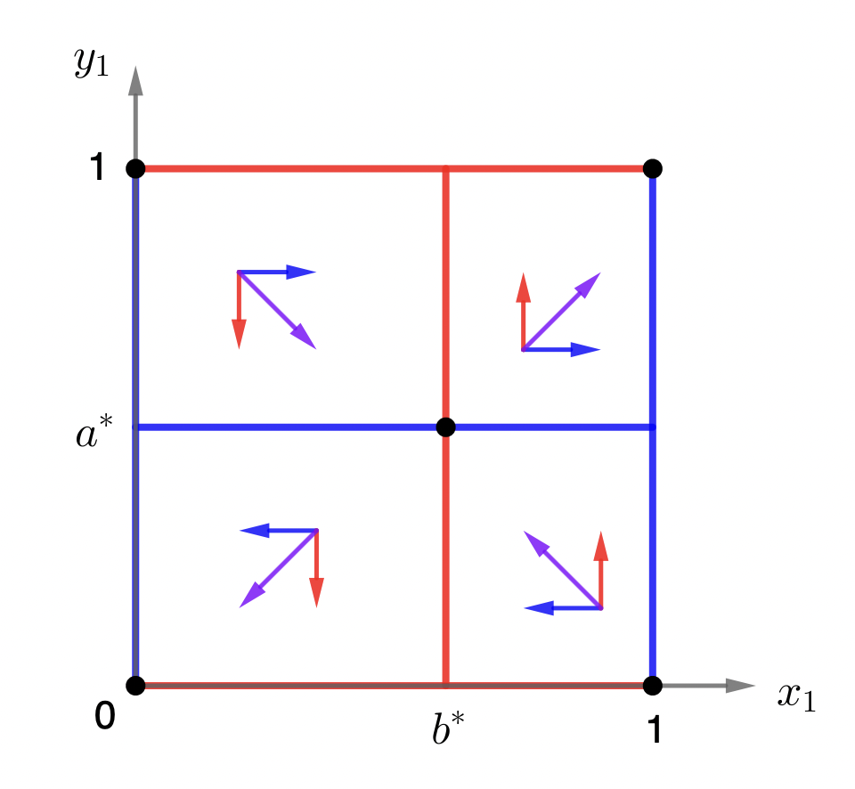
Refer to caption
Figure 3: Phase plot for positive diagonal matrices

If the matrices A=[a11a12a21a22]𝐴matrixsubscript𝑎11subscript𝑎12subscript𝑎21subscript𝑎22A=\begin{bmatrix}a_{11}&a_{12}\\ a_{21}&a_{22}\end{bmatrix} and B=[b11b12b21b22]𝐵matrixsubscript𝑏11subscript𝑏12subscript𝑏21subscript𝑏22B=\begin{bmatrix}b_{11}&b_{12}\\ b_{21}&b_{22}\end{bmatrix} are also positive diagonal matrices, then for times kT+T/2t<(k+1)T,k=0,1,2,formulae-sequence𝑘𝑇𝑇2𝑡𝑘1𝑇𝑘012kT+T/2\leq t<(k+1)T,k=0,1,2,\dots, we have the same qualitative phase portrait as Fig. 3.

If we want the probabilities/proportions to oscillate around the coexistence equilibrium (b,a)superscript𝑏superscript𝑎(b^{*},a^{*}), the qualitative phase portrait should look like Fig. 4.
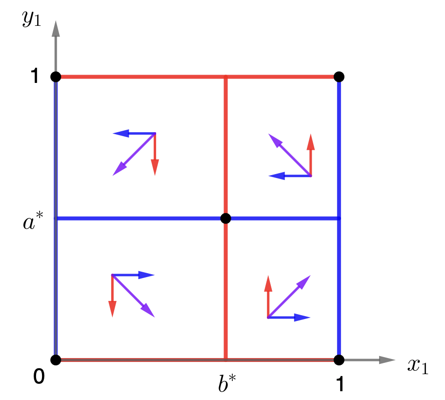
Refer to caption
Figure 4: Oscillation around coexistence

For such a phase portrait, we need 0<a,b<1formulae-sequence0superscript𝑎superscript𝑏10<a^{*},b^{*}<1 and also

a11(t)+a22(t)a12(t)a21(t)<0,subscript𝑎11𝑡subscript𝑎22𝑡subscript𝑎12𝑡subscript𝑎21𝑡0a_{11}(t)+a_{22}(t)-a_{12}(t)-a_{21}(t)<0,
b11(t)+b22(t)b12(t)b21(t)>0.subscript𝑏11𝑡subscript𝑏22𝑡subscript𝑏12𝑡subscript𝑏21𝑡0b_{11}(t)+b_{22}(t)-b_{12}(t)-b_{21}(t)>0.

Solve all four inequalities, we get

a11(t)<a21(t),a22(t)<a12(t);formulae-sequencesubscript𝑎11𝑡subscript𝑎21𝑡subscript𝑎22𝑡subscript𝑎12𝑡a_{11}(t)<a_{21}(t),a_{22}(t)<a_{12}(t);
b11(t)>b12(t),b22(t)>b21(t).formulae-sequencesubscript𝑏11𝑡subscript𝑏12𝑡subscript𝑏22𝑡subscript𝑏21𝑡b_{11}(t)>b_{12}(t),b_{22}(t)>b_{21}(t).

These are the conditions for an oscillatory system around the coexistence equilibrium. In this case the coexistence equilibrium is a center.

5 Trapping Regions

Assume we have two different saddle points under environment matrices MIsubscript𝑀𝐼M_{I} and MIIsubscript𝑀𝐼𝐼M_{II}. We wish to do what we did with the one dimensional examples, achieve trapping between the two unstable fixed points by switching between the two environments.

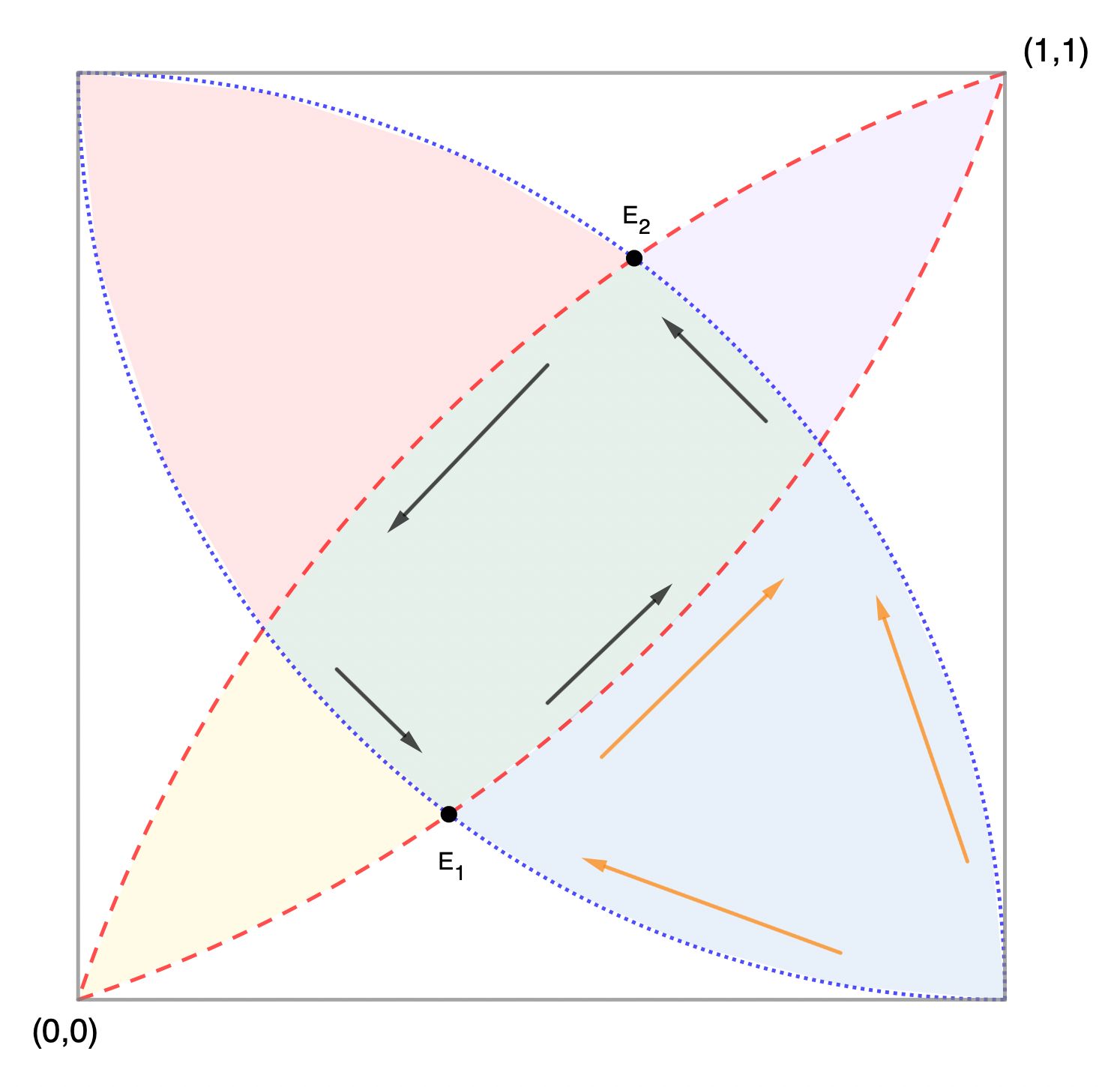
Let’s draw a qualitative phase portrait. Assume (0,0)00(0,0) and (1,1)11(1,1) are always stable, we have E1subscript𝐸1E_{1} as the saddle point for environment MIsubscript𝑀𝐼M_{I} and E2subscript𝐸2E_{2} as the saddle point for environment MIIsubscript𝑀𝐼𝐼M_{II}.

Refer to caption
Figure 5: Trapping Region

Here the blue dense dotted lines represent the stable manifold for the saddle points and the red sparse dotted lines represent the unstable manifolds. Then as long as the blue lines and red lines form a region bounded by alternating colored edges, we have a trapping region, shaded in green in Fig. 5. This is because, qualitatively, under environment I, the movements of points inside the region are marked by the two lower arrows, and when we switch to environment II, the movements of points inside the region are marked by the two upper arrows. Together they form a closed circular motion. As long as we make sure to switch the environment before the points moves out the boundary of the region, they should be trapped in the region forever.

Now let’s look at the blue shaded region instead. Unlike the green region, along the boundaries of the blue region, the three orange arrows don’t form a consecutive circular path. Indeed, when under environment I, the movements of points inside the blue region should follow the two orange arrows to the left, and if we don’t ever switch the environment, the points will escape the blue region from the right. Now if we switch the environment before the points escape, they will now follow the orange arrow on the right. If we stay on environment II for long enough the points will move on into the green region and escape the blue region. If we manage to switch back to environment I before points move into the green region, well, they will keep moving right until they escape the blue region on the right.

This analysis can be applied to the purple, pink, and yellow regions as well. We can have a trapping region if and only if the arrows along the boundary form a closed circular path.

6 Linearization of the system

Although we don’t have explicit solutions for our nonlinear system, we can still linearize it near the fixed point (b,a)superscript𝑏superscript𝑎(b^{*},a^{*}).

[x1y1]=[0αβ0]([x1y1][ba]),superscriptmatrixsubscript𝑥1subscript𝑦1matrix0𝛼𝛽0matrixsubscript𝑥1subscript𝑦1matrixsuperscript𝑏superscript𝑎\begin{bmatrix}x_{1}\\ y_{1}\end{bmatrix}^{\prime}=\begin{bmatrix}0&\alpha\\ \beta&0\end{bmatrix}(\begin{bmatrix}x_{1}\\ y_{1}\end{bmatrix}-\begin{bmatrix}b^{*}\\ a^{*}\end{bmatrix}), (18)

here

α=b(1b)[a11(t)+a22(t)a12(t)a21(t)],𝛼superscript𝑏1superscript𝑏delimited-[]subscript𝑎11𝑡subscript𝑎22𝑡subscript𝑎12𝑡subscript𝑎21𝑡\alpha=b^{*}(1-b^{*})[a_{11}(t)+a_{22}(t)-a_{12}(t)-a_{21}(t)],
β=a(1a)[b11(t)+b22(t)b12(t)b21(t)].𝛽superscript𝑎1superscript𝑎delimited-[]subscript𝑏11𝑡subscript𝑏22𝑡subscript𝑏12𝑡𝑏21𝑡\beta=a^{*}(1-a^{*})[b_{11}(t)+b_{22}(t)-b_{12}(t)-b{21}(t)].

Still assuming we have a system that switches between environments
MI=ABsubscript𝑀𝐼direct-sum𝐴𝐵M_{I}=A\oplus B and MII=ABsubscript𝑀𝐼𝐼direct-sumsuperscript𝐴superscript𝐵M_{II}=A^{\prime}\oplus B^{\prime}. Here A=[a11a12a21a22],B=[b11b12b21b22],A=[a11a12a21a22],B=[b11b12b21b22]formulae-sequence𝐴matrixsubscript𝑎11subscript𝑎12subscript𝑎21subscript𝑎22formulae-sequence𝐵matrixsubscript𝑏11subscript𝑏12subscript𝑏21subscript𝑏22formulae-sequencesuperscript𝐴matrixsuperscriptsubscript𝑎11superscriptsubscript𝑎12superscriptsubscript𝑎21superscriptsubscript𝑎22superscript𝐵superscriptmatrixsuperscriptsubscript𝑏11superscriptsubscript𝑏12superscriptsubscript𝑏21superscriptsubscript𝑏22A=\begin{bmatrix}a_{11}&a_{12}\\ a_{21}&a_{22}\end{bmatrix},B=\begin{bmatrix}b_{11}&b_{12}\\ b_{21}&b_{22}\end{bmatrix},\\ A^{\prime}=\begin{bmatrix}a_{11}^{\prime}&a_{12}^{\prime}\\ a_{21}^{\prime}&a_{22}^{\prime}\end{bmatrix},B^{\prime}=\begin{bmatrix}b_{11}^{\prime}&b_{12}^{\prime}\\ b_{21}^{\prime}&b_{22}^{\prime}\end{bmatrix}^{\prime} are all constant matrices. Now assume

a=a22a12a11+a22a12a21,superscript𝑎subscript𝑎22subscript𝑎12subscript𝑎11subscript𝑎22subscript𝑎12subscript𝑎21\displaystyle a^{*}=\frac{a_{22}-a_{12}}{a_{11}+a_{22}-a_{12}-a_{21}},
b=b22b21b11+b22b12b21,superscript𝑏subscript𝑏22subscript𝑏21subscript𝑏11subscript𝑏22subscript𝑏12subscript𝑏21\displaystyle b^{*}=\frac{b_{22}-b_{21}}{b_{11}+b_{22}-b_{12}-b_{21}},
c=a22a12a11+a22a12a21,superscript𝑐superscriptsubscript𝑎22superscriptsubscript𝑎12superscriptsubscript𝑎11superscriptsubscript𝑎22superscriptsubscript𝑎12superscriptsubscript𝑎21\displaystyle c^{*}=\frac{a_{22}^{\prime}-a_{12}^{\prime}}{a_{11}^{\prime}+a_{22}^{\prime}-a_{12}^{\prime}-a_{21}^{\prime}},
d=b22b21b11+b22b12b21;superscript𝑑superscriptsubscript𝑏22superscriptsubscript𝑏21superscriptsubscript𝑏11superscriptsubscript𝑏22superscriptsubscript𝑏12superscriptsubscript𝑏21\displaystyle d^{*}=\frac{b_{22}^{\prime}-b_{21}^{\prime}}{b_{11}^{\prime}+b_{22}^{\prime}-b_{12}^{\prime}-b_{21}^{\prime}};
α=b(1b)(a11+a22a12a21),𝛼superscript𝑏1superscript𝑏subscript𝑎11subscript𝑎22subscript𝑎12subscript𝑎21\displaystyle\alpha=b^{*}(1-b^{*})(a_{11}+a_{22}-a_{12}-a_{21}),
β=a(1a)(b11+b22b12b21),𝛽superscript𝑎1superscript𝑎subscript𝑏11subscript𝑏22subscript𝑏12subscript𝑏21\displaystyle\beta=a^{*}(1-a^{*})(b_{11}+b_{22}-b_{12}-b_{21}),
α=d(1d)(a11+a22a12a21),superscript𝛼superscript𝑑1superscript𝑑superscriptsubscript𝑎11superscriptsubscript𝑎22superscriptsubscript𝑎12superscriptsubscript𝑎21\displaystyle\alpha^{\prime}=d^{*}(1-d^{*})(a_{11}^{\prime}+a_{22}^{\prime}-a_{12}^{\prime}-a_{21}^{\prime}),
β=c(1c)(b11+b22b12b21).superscript𝛽superscript𝑐1superscript𝑐superscriptsubscript𝑏11superscriptsubscript𝑏22superscriptsubscript𝑏12superscriptsubscript𝑏21\displaystyle\beta^{\prime}=c^{*}(1-c^{*})(b_{11}^{\prime}+b_{22}^{\prime}-b_{12}^{\prime}-b_{21}^{\prime}).

Under environment MIsubscript𝑀𝐼M_{I}, the linear system of ODEs has solutions

[x1y1]=[ba]+c1eαβt[αβ]+c2eαβt[αβ].matrixsubscript𝑥1subscript𝑦1matrixsuperscript𝑏superscript𝑎subscript𝑐1superscript𝑒𝛼𝛽𝑡matrix𝛼𝛽subscript𝑐2superscript𝑒𝛼𝛽𝑡matrix𝛼𝛽\begin{bmatrix}x_{1}\\ y_{1}\end{bmatrix}=\begin{bmatrix}b^{*}\\ a^{*}\end{bmatrix}+c_{1}e^{\sqrt{\alpha\beta}t}\begin{bmatrix}\sqrt{\alpha}\\ \sqrt{\beta}\end{bmatrix}+c_{2}e^{-\sqrt{\alpha\beta}t}\begin{bmatrix}\sqrt{\alpha}\\ -\sqrt{\beta}\end{bmatrix}.

And under environment MIIsubscript𝑀𝐼𝐼M_{II}, this linear system of ODEs has solutions

[x1y1]=[dc]+c1eαβt[αβ]+c2eαβt[αβ].matrixsubscript𝑥1subscript𝑦1matrixsuperscript𝑑superscript𝑐subscript𝑐1superscript𝑒superscript𝛼superscript𝛽𝑡matrixsuperscript𝛼superscript𝛽subscript𝑐2superscript𝑒superscript𝛼superscript𝛽𝑡matrixsuperscript𝛼superscript𝛽\begin{bmatrix}x_{1}\\ y_{1}\end{bmatrix}=\begin{bmatrix}d^{*}\\ c^{*}\end{bmatrix}+c_{1}e^{\sqrt{\alpha^{\prime}\beta^{\prime}}t}\begin{bmatrix}\sqrt{\alpha^{\prime}}\\ \sqrt{\beta^{\prime}}\end{bmatrix}+c_{2}e^{-\sqrt{\alpha^{\prime}\beta^{\prime}}t}\begin{bmatrix}\sqrt{\alpha^{\prime}}\\ -\sqrt{\beta^{\prime}}\end{bmatrix}.

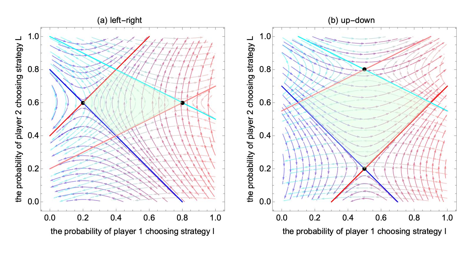
The fixed points E1=(b,a),E2=(d,c)formulae-sequencesubscript𝐸1superscript𝑏superscript𝑎subscript𝐸2superscript𝑑superscript𝑐E_{1}=(b^{*},a^{*}),E_{2}=(d^{*},c^{*}) are saddle points. Notice that their two eigenvector directions are symmetric by the y𝑦y-axis. If the two fixed points are positioned as in Fig. 6(a), then the green shaded region is a trapping region. Here the blue and light blue straight lines represent the contracting directions, or stable manifolds and the red and pink lines represent expanding directions, or unstable manifolds.
Refer to caption
Figure 6: Linear Trapping: no shared manifolds

To have this left-right configuration, we need

|acbd|<min{βα,βα}.superscript𝑎superscript𝑐superscript𝑏superscript𝑑𝛽𝛼superscript𝛽superscript𝛼\displaystyle\left|\frac{a^{*}-c^{*}}{b^{*}-d^{*}}\right|<\min\{\sqrt{\frac{\beta}{\alpha}},\sqrt{\frac{\beta^{\prime}}{\alpha^{\prime}}}\}. (19)

The contracting and expanding directions of E1subscript𝐸1E_{1} divides our phase space into 4 parts. We should have 4 configurations with a convex quadrilateral trapping region. Only 2 of these are distinct considering symmetry between E1subscript𝐸1E_{1} and E2subscript𝐸2E_{2}, we can always rename or relabel them. The other distinct configuration, the up-down configuration in Fig. 6 (b) requires

|acbd|>max{βα,βα}.superscript𝑎superscript𝑐superscript𝑏superscript𝑑𝛽𝛼superscript𝛽superscript𝛼\displaystyle\left|\frac{a^{*}-c^{*}}{b^{*}-d^{*}}\right|>\max\{\sqrt{\frac{\beta}{\alpha}},\sqrt{\frac{\beta^{\prime}}{\alpha^{\prime}}}\}. (20)

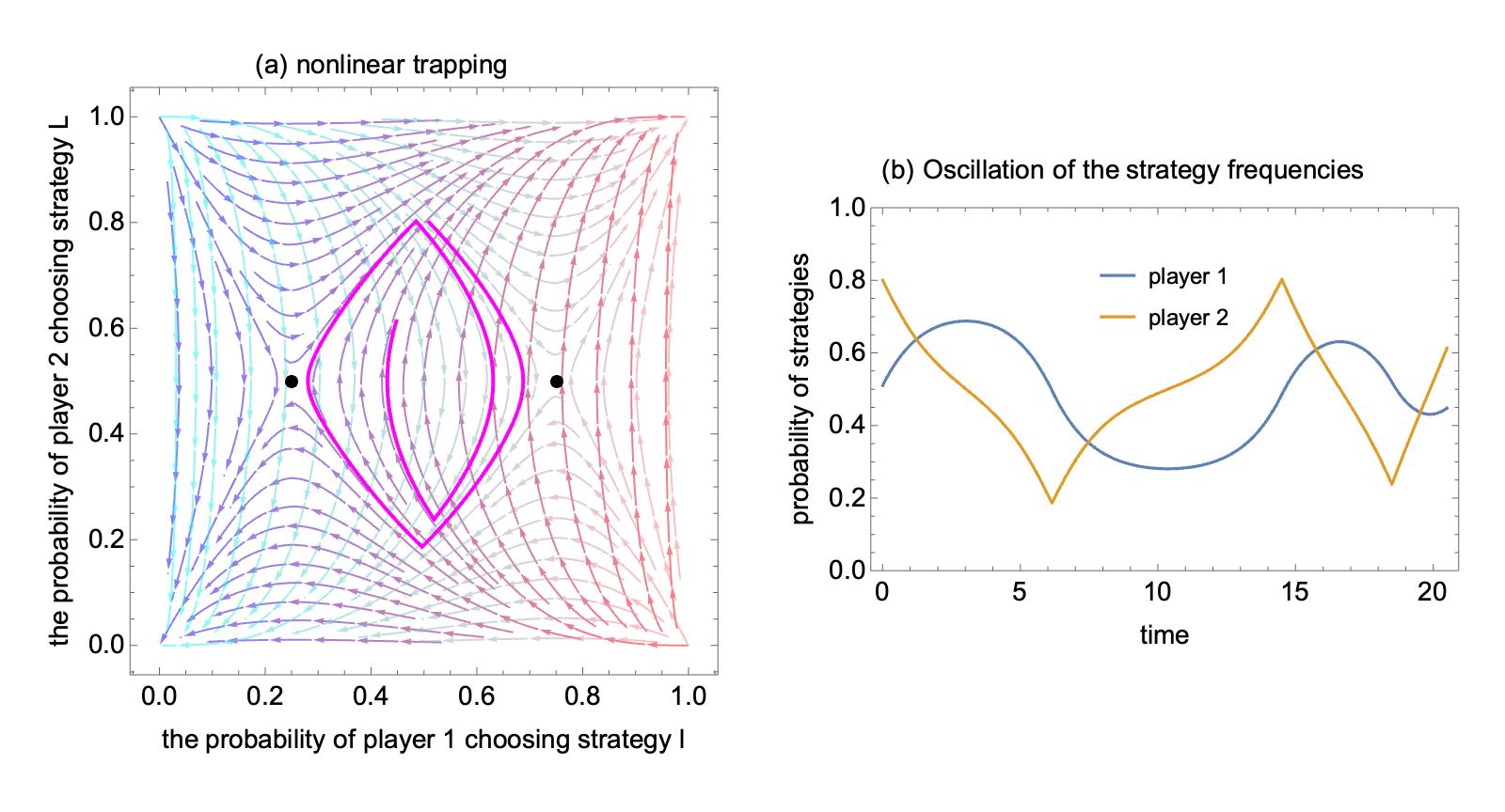
To show that this linear approximation actually is close enough to the nonlinear system, we study a specific nonlinear system here as well. The trapping region in Fig. 7(a) is not a convex quadrilateral any more, we plot a specific trapping trajectory in magenta and the corresponding frequencies of strategies in Fig.7(b). The equations for this nonlinear system are

{x=x(1x)(2y1),y=y(1y)(4x3).casessuperscript𝑥𝑥1𝑥2𝑦1otherwisesuperscript𝑦𝑦1𝑦4𝑥3otherwise\begin{cases}x^{\prime}=x(1-x)(2y-1),\\ y^{\prime}=y(1-y)(4x-3).\end{cases} (21)
{x=x(1x)(2y1),y=y(1y)(4x1).casessuperscript𝑥𝑥1𝑥2𝑦1otherwisesuperscript𝑦𝑦1𝑦4𝑥1otherwise\begin{cases}x^{\prime}=x(1-x)(2y-1),\\ y^{\prime}=y(1-y)(4x-1).\end{cases} (22)
Refer to caption
Figure 7: Nonlinear Trapping

At time t0=0subscript𝑡00t_{0}=0, we start with (21), and initial conditions x0=0.51,y0=0.8formulae-sequencesubscript𝑥00.51subscript𝑦00.8x_{0}=0.51,y_{0}=0.8. We switch over to (22) at t1=6.15subscript𝑡16.15t_{1}=6.15. Then after t2=8.35subscript𝑡28.35t_{2}=8.35 we switch again, and the trajectory in magenta happens when we switch again after t3=4subscript𝑡34t_{3}=4 and t4=2subscript𝑡42t_{4}=2. The corresponding solutions x(t)𝑥𝑡x(t) and y(t)𝑦𝑡y(t) are plotted here as well (Fig. 7). We can see the curve for x(t)𝑥𝑡x(t) is rather smooth while the curve for y(t)𝑦𝑡y(t) has sharp tips. This is because the equation for x(t)𝑥𝑡x(t) actually stays the same between the two environments.

This example is rather simple but it is nonlinear, and it corresponds very well to the left-right linear trapping region (Fig. 6 (a)). Given this resemblance, we have a good reason to think the linear trapping regions, although not exactly what we will see in realistic nonlinear systems, still give us reasonable approximation in nonlinear trapping.

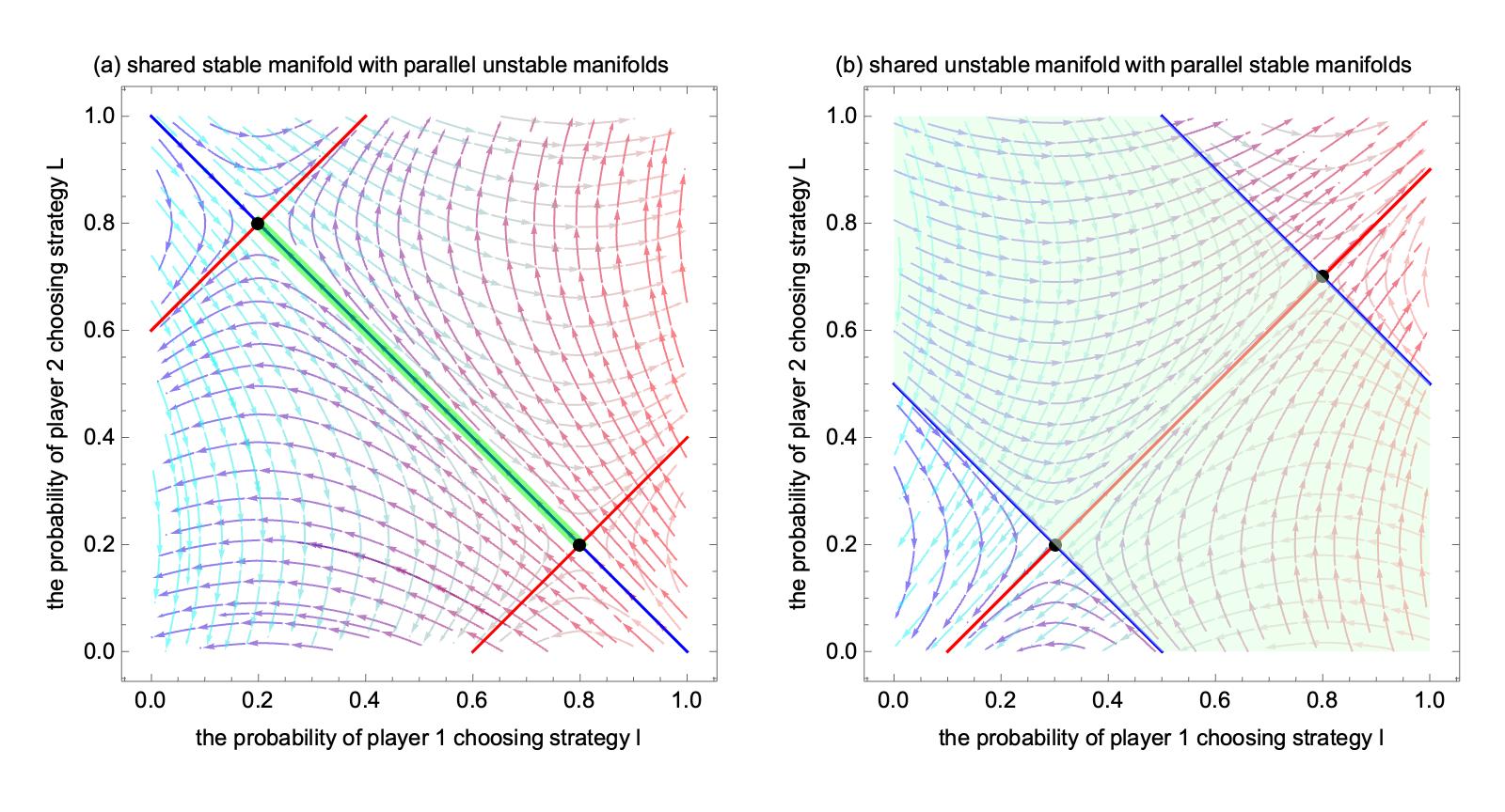
In addition to the left-right and up-down configurations in Fig. 6, if E2subscript𝐸2E_{2} lies on the stable or unstable manifold of E1subscript𝐸1E_{1}, or the other way around, we will also have a trapping region. These cases, co require

|acbd|=βα or βα.superscript𝑎superscript𝑐superscript𝑏superscript𝑑𝛽𝛼 or superscript𝛽superscript𝛼\displaystyle\left|\frac{a^{*}-c^{*}}{b^{*}-d^{*}}\right|=\sqrt{\frac{\beta}{\alpha}}\text{ or }\sqrt{\frac{\beta^{\prime}}{\alpha^{\prime}}}. (23)
Refer to caption
Figure 8: Linear Trapping: shared manifold with parallel other manifolds

In Fig. 8, we have the very special case where one fixed point is on the stable, or unstable manifold of the other fixed point, and their other manifolds are parallel to each other. When one fixed point is on the stable manifold of the other, the trapping region degenerates to a line segment between the two fixed points. While when one fixed point is on the unstable manifold of the other, the trapping region becomes much larger and takes up a big part of our phase space.
Refer to caption
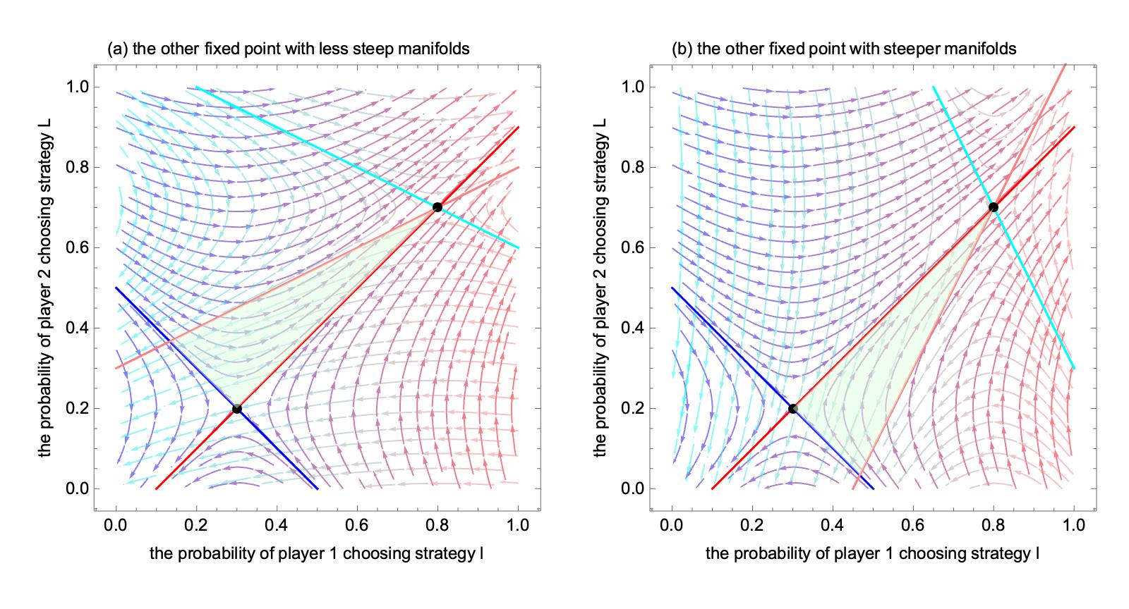
Figure 9: Linear Trapping: one fixed point on the unstable manifold of the other

Still considering one fixed point on the stable or unstable manifold of the other fixed point, we now focus on the cases where their other manifolds are not parallel to each other. In Fig. 9, one fixed point is on the unstable manifold of the other fixed point, depending on whether the manifolds of the fixed point are less steep or steeper, we have two slightly different triangular trapping regions. And in Fig. 10, one fixed point is on the stable manifold of the other fixed point. We end up with similar triangular trapping regions.
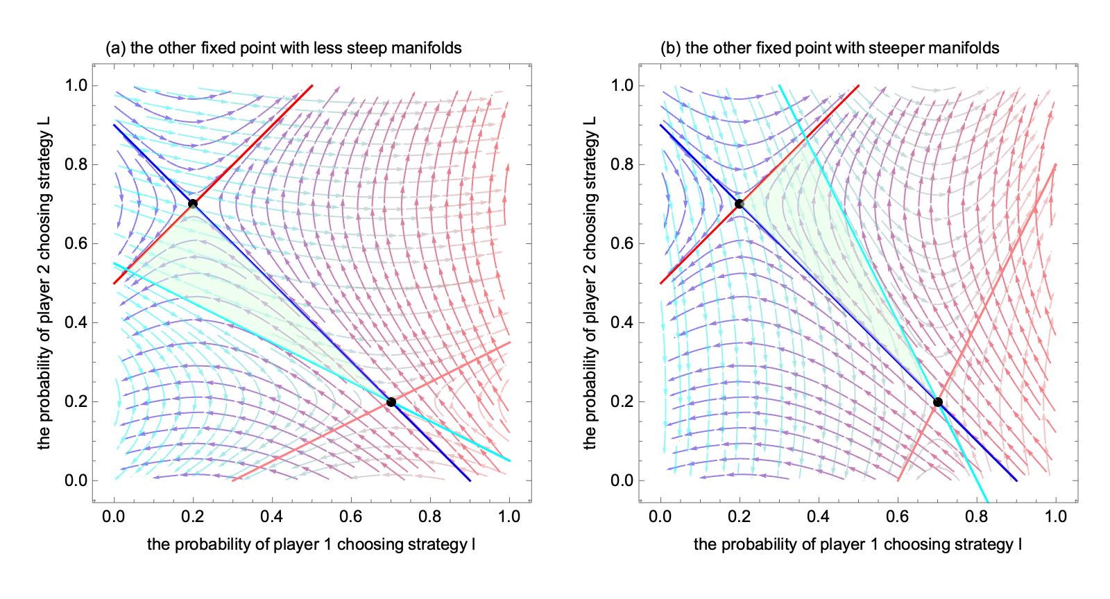
Refer to caption
Figure 10: Linear Trapping: one fixed point on the stable manifold of the other

One might ask, what happens when

min{βα,βα}<|acbd|<max{βα,βα}?𝛽𝛼superscript𝛽superscript𝛼superscript𝑎superscript𝑐superscript𝑏superscript𝑑𝛽𝛼superscript𝛽superscript𝛼?\displaystyle\min\{\sqrt{\frac{\beta}{\alpha}},\sqrt{\frac{\beta^{\prime}}{\alpha^{\prime}}}\}<\left|\frac{a^{*}-c^{*}}{b^{*}-d^{*}}\right|<\max\{\sqrt{\frac{\beta}{\alpha}},\sqrt{\frac{\beta^{\prime}}{\alpha^{\prime}}}\}? (24)

Notice that (19),(20),(23) and (24) include all possible configurations of the two distinct fixed points E1subscript𝐸1E_{1} and E2subscript𝐸2E_{2}. In the case of (24) we still have trapping regions but they are a little more complicated than the convex trapping regions we have shown so far.

Whenever we have the slope of the segment E1E2subscript𝐸1subscript𝐸2E_{1}E_{2} smaller than the eigenvector slope of E1subscript𝐸1E_{1}, that means E2subscript𝐸2E_{2} is either on the left or the right of the 4 parts of the phase space divided by the contracting and expanding directions of E1subscript𝐸1E_{1}. This is why (19) corresponds to the case when E1subscript𝐸1E_{1} and E2subscript𝐸2E_{2} are in the ”left-right” configuration for each other. Similarly (20) corresponds to when the two fixed points are in the ”up-down” configuration for each other. Intuitively (24) means E1subscript𝐸1E_{1} is in the ”left-right” configuration w.r.t. E2subscript𝐸2E_{2} while E2subscript𝐸2E_{2} is in the ”up-down” configuration w.r.t. E1subscript𝐸1E_{1}, or the other way around. We draw two different examples in Fig. 11.
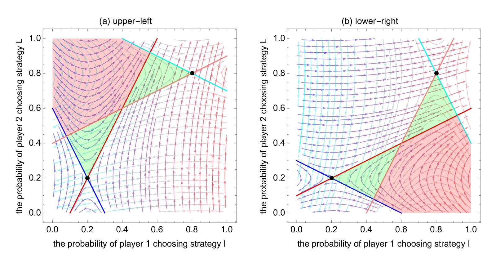
Refer to caption
Figure 11: Linear Trapping: mixed configuration for fixed points positions

Here we have a slightly more complicated mode of trapping. For example, in Fig. 11(a) each of the green triangular regions on their own is a trapping region. But the red shaded region combined with the two green triangles is also a trapping region. When we consider the combined shape, which is not convex any more, we could end up with a trapped loop that forms a butterfly shape or ”8” shape. The trajectory starts in the red region, shoots into one of the green ears and then returns to the red region. If we switch the governing equations in time, then the trajectory is going to shoot into the other green ear and return to the red region. Although Fig. 11(a) and (b) have different locations for the trapping regions, the dynamics is the same. The phase portraits for cases where the red region is located at the upper-right corner and lower-left corner can also be drawn but we leave that up for the readers.

For the sake of completeness, we also put a simplified sketch of all possible linear trapping regions in Fig. 12 below. We only draw the upper-left location trapping for the mixed configuration.

Figure 12: All cases for linear trapping

7 Constant of motion for the system

Our system is governed by these equations

{x˙1=x1(1x1){[a11(t)+a22(t)a12(t)a21(t)]y1[a22(t)a12(t)]},y˙1=y1(1y1){[b11(t)+b22(t)b12(t)b21(t)]x1[b22(t)b21(t)]}.casessubscript˙𝑥1subscript𝑥11subscript𝑥1delimited-[]subscript𝑎11𝑡subscript𝑎22𝑡subscript𝑎12𝑡subscript𝑎21𝑡subscript𝑦1delimited-[]subscript𝑎22𝑡subscript𝑎12𝑡otherwisesubscript˙𝑦1subscript𝑦11subscript𝑦1delimited-[]subscript𝑏11𝑡subscript𝑏22𝑡subscript𝑏12𝑡subscript𝑏21𝑡subscript𝑥1delimited-[]subscript𝑏22𝑡subscript𝑏21𝑡otherwise\begin{cases}\dot{x}_{1}=x_{1}(1-x_{1})\{[a_{11}(t)+a_{22}(t)-a_{12}(t)-a_{21}(t)]y_{1}-[a_{22}(t)-a_{12}(t)]\},\\ \dot{y}_{1}=y_{1}(1-y_{1})\{[b_{11}(t)+b_{22}(t)-b_{12}(t)-b_{21}(t)]x_{1}-[b_{22}(t)-b_{21}(t)]\}.\end{cases}

For convenience, let’s assume aij,bijsubscript𝑎𝑖𝑗subscript𝑏𝑖𝑗a_{ij},b_{ij}’s are constants here, for i,j=1,2formulae-sequence𝑖𝑗12i,j=1,2. Let p=a11+a22a12a21𝑝subscript𝑎11subscript𝑎22subscript𝑎12subscript𝑎21p=a_{11}+a_{22}-a_{12}-a_{21}, q=a22a12𝑞subscript𝑎22subscript𝑎12q=a_{22}-a_{12}, u=b11+b22b12b21𝑢subscript𝑏11subscript𝑏22subscript𝑏12subscript𝑏21u=b_{11}+b_{22}-b_{12}-b_{21}, v=b22b21𝑣subscript𝑏22subscript𝑏21v=b_{22}-b_{21}. We will write x𝑥x for x1subscript𝑥1x_{1}, y𝑦y for y1subscript𝑦1y_{1} in the following solving process to make the symbols easier to read and write.

Our system becomes

x˙=x(1x)(pyq),˙𝑥𝑥1𝑥𝑝𝑦𝑞\dot{x}=x(1-x)(py-q),
y˙=y(1y)(uxv).˙𝑦𝑦1𝑦𝑢𝑥𝑣\dot{y}=y(1-y)(ux-v).

Divide the second equation by the first, we get

dydx=y(1y)(uxv)x(1x)(pyq).𝑑𝑦𝑑𝑥𝑦1𝑦𝑢𝑥𝑣𝑥1𝑥𝑝𝑦𝑞\displaystyle\frac{dy}{dx}=\frac{y(1-y)(ux-v)}{x(1-x)(py-q)}.

This is a separable equation.

(pyq)dyy(1y)=(pq1yqy)dy=(uxv)dxx(1x)=(uv1xvx)dx,𝑝𝑦𝑞𝑑𝑦𝑦1𝑦𝑝𝑞1𝑦𝑞𝑦𝑑𝑦𝑢𝑥𝑣𝑑𝑥𝑥1𝑥𝑢𝑣1𝑥𝑣𝑥𝑑𝑥\displaystyle\frac{(py-q)dy}{y(1-y)}=(\frac{p-q}{1-y}-\frac{q}{y})dy=\frac{(ux-v)dx}{x(1-x)}=(\frac{u-v}{1-x}-\frac{v}{x})dx,
(qp)ln(1y)qlny=(vu)ln(1x)vlnx+c,𝑞𝑝1𝑦𝑞𝑦𝑣𝑢1𝑥𝑣𝑥𝑐\displaystyle(q-p)\ln(1-y)-q\ln y=(v-u)\ln(1-x)-v\ln x+c,
(1y)qpyq=c(1x)vuxv,xv(1y)qp=cyq(1x)vu,formulae-sequencesuperscript1𝑦𝑞𝑝superscript𝑦𝑞𝑐superscript1𝑥𝑣𝑢superscript𝑥𝑣superscript𝑥𝑣superscript1𝑦𝑞𝑝𝑐superscript𝑦𝑞superscript1𝑥𝑣𝑢\displaystyle\frac{(1-y)^{q-p}}{y^{q}}=c\frac{(1-x)^{v-u}}{x^{v}},x^{v}(1-y)^{q-p}=cy^{q}(1-x)^{v-u},
V(x,y)=xv(1x)uvyq(1y)qp=c𝑉𝑥𝑦superscript𝑥𝑣superscript1𝑥𝑢𝑣superscript𝑦𝑞superscript1𝑦𝑞𝑝𝑐\displaystyle V(x,y)=x^{v}(1-x)^{u-v}y^{-q}(1-y)^{q-p}=c

V(x,y)=c𝑉𝑥𝑦𝑐V(x,y)=c is a constant of motion [28] for our system. It gives the analytic implicit solution to our system. Without an explicit solution, we still don’t have the exact behavior of x(t)𝑥𝑡x(t) and y(t)𝑦𝑡y(t).

8 Discussion

Understanding how cooperative traits are maintained in populations is an essential problem of deep importance not only in evolutionary biology, but also in microbial ecology and systems biology. Ecological factors such as population density, disturbance frequency, population dispersal, resource supply, spatial structuring of populations, the presence of mutualisms, or the presence of a competing species in the environment, often play an important role in the evolution of cooperation. The effect that these and other ecological factors play on the evolution of cooperation is in general well understood. However, the reverse process, i.e., the effect that the evolution of cooperative traits may have on the ecological properties of populations is worthy of investigation using the framework of eco-evolutionary dynamics.

In this paper we considered eco-evolutionary games that incorporate the impact of switching environment on game dynamics. We consider a changing environment, which is represented as a switched system between two different payoff matrices. Motivated by the study of the tragedy of the commons in evolutionary biology, we demonstrate how alternative dynamics can arise. By switching between two environments, we can achieve an oscillating dynamic equilibrium and maintain coexistence which is impossible otherwise. Cooperators and defectors can coexist if the system state does not exceed the trapping regions.

Our model uses simplifying assumptions and is just a first step toward a more sophisticated eco-evolutionary model [29, 30]. Still, we strongly believe that our results provide valuable insights in designing control mechanisms. We may consider relaxing or extending these simplifying assumptions for future research. For example, instead of a switch between two different payoff matrices, we could consider a linear combination of the two. The possibilities under a general nonlinear payoff matrix are likely even broader. We could also consider incorporating multiplayer games into our current model toward a more realistic description of population dynamics.

Other possible extensions of our work could be to consider feedback between strategies and patch quality [31, 32], where not all players experience the same environment. Negative environmental feedback gives immediate benefits in rich environments but results in net costs in poor environments.

In the analysis of the trapping regions we find multiple segments of stable and unstable manifolds in phase graphs, which is a new dynamical phenomenon that is different from interior fixed equilibrium situation obtained in previous works. We provide constructive specific control examples where the system states evolve contained inside the trapping regions. In some very special cases we even get an equilibrium manifold, depending on the initial condition, our system could be trapped on the equilibrium manifold. This combination of eco-evolutionary dynamics and control theory result could be used to help steer the population to desired states in social dilemma games. Although our present study is focused on mixed strategy bimatrix games, system properties are unchanged in a small neighbourhood, our results on control can be generalized to many other important situations.

Acknowledgements

F.F. is supported by the Bill & Melinda Gates Foundation (award no. OPP1217336), the NIH COBRE Program (grant no. 1P20GM130454), a Neukom CompX Faculty Grant, the Dartmouth Faculty Startup Fund, and the Walter & Constance Burke Research Initiation Awar d.

References

  • [1] C. Hauret, G. Szabó, Game theory and physics, American Journal of Physics 73 (5) (2005) 405-414.
  • [2] M. A. Nowak, Evolutionary dynamics: exploring the equations of life, Harvard University Press, 2006.
  • [3] C. P. Roca, J. A. Cuesta, A. Sánchez, Evolutionary game theory: Temporal and spatial effects beyond replicator dynamics, Physics of life reviews 6 (4) (2009) 208-249.
  • [4] R. Cressman, Y. Tao, The replicator equation and other game dynamics, Proceedings of the National Academy of Sciences 111 (supplement 3) (2014) 10810-10817.
  • [5] M. Perc, A. Szolnoki, Coevolutionary games-a mini review, BioSystems 99 (2) (2010) 109-125.
  • [6] A. Sánchez, J. Gore, Feedback between population and evolutionary dynamics determines the fate of social microbial populations, PLoS biology 11 (4) (2013) e1001547.
  • [7] X. Wang, Z. Zhang, F. Fu, Steering eco-evolutionary game dynamics with manifold control, Proceedings of the Royal Society A 476 (2233) (2020) 20190643.
  • [8] S. Estrela, E. Libby, J. Van Cleve, F. Débarre, M. Deforet, W. R. Harcombe, J. Peña, S. P. Brown, M. E. Hochberg, Environmentally mediated social dilemmas, Trends in ecology & evolution 34 (1) (2019) 6-18.
  • [9] D. A. Rand, A. Raju, M. Saez, F. Corson, E. D. Siggia, Geometry of gene regulatory dynamics, arXiv preprint arXiv:2105.13722 (2021).
  • [10] J. S. Weitz, C. Eksin, K. Paarporn, S. P. Brown, W. C. Ratcliff, An oscillating tragedy of the commons in replicator dynamics with game-environment feedback, Proceedings of the National Academy of Sciences 113 (47) (2016) E7518-E7525.
  • [11] C. Hilbe, Š. Šimsa, K. Chatterjee, M. A. Nowak, Evolution of cooperation in stochastic games, Nature 559 (7713) (2018) 246-249.
  • [12] X. Chen, A. Szolnoki, Punishment and inspection for governing the commons in a feedback-evolving game, PLoS computational biology 14 (7) (2018) e1006347.
  • [13] Y. Shao, X. Wang, F. Fu, Evolutionary dynamics of group cooperation with asymmetrical environmental feedback, EPL (Europhysics Letters) 126 (4) (2019) 40005.
  • [14] C. Hauert, C. Saade, A. McAvoy, Asymmetric evolutionary games with environmental feedback, Journal of theoretical biology 462 (2019) 347-360.
  • [15] A. R. Tilman, J. B. Plotkin, E. Akçay, Evolutionary games with environmental feedbacks, Nature communications 11 (1) (2020) 1-11.
  • [16] G. Hardin, The tragedy of the commons: the population problem has no technical solution; it requires a fundamental extension in morality, Science 162 (3859) (1968) 1243-1248.
  • [17] T. Wu, F. Fu, L. Wang, Coevolutionary dynamics of aspiration and strategy in spatial repeated public goods games, New Journal of Physics 20 (6) (2018) 063007.
  • [18] H. Perez, C. Gracia-Lazaro, F. Dercole, Y. Moreno, Cooperation in costly-access environments, New Journal of Physics (2022).
  • [19] X. Wang, M. Perc, Replicator dynamics of public goods games with global exclusion, Chaos: An Interdisciplinary Journal of Nonlinear Science 32 (7) (2022) 073132.
  • [20] S. Wang, X. Chen, Z. Xiao, A. Szolnoki, Decentralized incentives for general well-being in networked public goods game, Applied Mathematics and Computation 431 (2022) 127308.
  • [21] C. E. Tarnita, The ecology and evolution of social behavior in microbes, Journal of Experimental Biology 220 (1) (2017) 18-24.
  • [22] A. Cardillo, N. Masuda, Critical mass effect in evolutionary games triggered by zealots, Physical Review Research 2 (2) (2020) 023305.
  • [23] X. Chen, F. Fu, Imperfect vaccine and hesteresis, Proceedings of the royal society B 286 (1894) (2019) 20182406.
  • [24] E. Ostrom, R. Gardner, Coping with asymmetries in the commons: self-governing irrigation systems can work, Journal of economic perspectives 7 (4) (1993) 93-112.
  • [25] X. Chen, F. Fu, Social learning of prescribing behavior can promote population optimum of antibiotic use, Frontiers in Physics 6 (2018) 139.
  • [26] L. Cao, B. Wu, Eco-evolutionary dynamics with payoff-dependent environmental feedback, Chaos, Solitons & Fractals 150 (2021) 111088.
  • [27] A. Glaubitz, F. Fu, Oscillatory dynamics in the dilemma of social distancing, Proceedings of the Royal Society A 476 (2243) (2020) 20200686.
  • [28] J. Hofbauer, K. Sigmund, Evolutionary Games and Population Dynamics, Cambridge University Press, 1998.
  • [29] A. R. Tilman, V. V. Vasconcelos, E. Akcay, J. B. Plotkin, The evolution of forecasting for decision making in dynamic environments, arXiv preprint arXiv:2108.00047 (2021).
  • [30] K. Jnawali, M. Anand, C. T. Bauch, Stochasticity-induced persistence in coupled social-ecological systems, Journal of Theoretical Biology 542 (2022) 111088.
  • [31] A. K. Fahimipour, F. Zeng, M. Homer, A. Traulsen, S. A. Levin, T. Gross, Sharp thresholds limit the benefit of defector avoidance in cooperation on networks, Proceedings of the National Academy of Sciences 119 (33) (2022) e2120120119.
  • [32] F. Liu, B. Wu, Environmental quality and population welfare in markovian eco-evolutionary dynamics, Applied Mathematics and Computation 431 (2022) 127309.