Physics implications of recent Dresden-II reactor data

Abstract

Prompted by the recent Dresden-II reactor data we examine its implications for the determination of the weak mixing angle, paying attention to the effect of the quenching function. We also determine the resulting constraints on the unitarity of the neutrino mixing matrix, as well as on the most general type of nonstandard neutral-current neutrino interactions.

1 Introduction

The neutral-current observation of neutrino events opens new windows that may reveal novel aspects of neutrino physics. Coherent elastic neutrino nucleus scattering (CE$\nu$NS) is a low-energy process, proposed by Freedman [1], where the entire nucleus is scattered off elastically by the neutrinos. Despite the large predicted CE$\nu$NS cross section, its detection faces experimental challenges mainly because of the very tiny nuclear recoil signals produced in the aftermath of a CE$\nu$NS event. CE$\nu$NS was first observed at the Oak Ridge National Laboratory by the COHERENT Collaboration which exploited the $\pi$-DAR (pion-decay-at-rest) neutrino beam coming from the Spallation Neutron Source facility (SNS) using a CsI detector [2, 3] and subsequently using a liquid argon detector [4]. Nuclear power plants constitute another important experimental probe for CE$\nu$NS studies, with several experiments currently underway such as CONNIE [5], CONUS [6, 7] and $\nu$GEN [8] or in preparation (e.g. MINER [9], RICOCHET [10], $\nu$-cleus [11], TEXONO [12], $\nu$IOLETA [13] and Scintillating Bubble Chamber (SBC) [14]). These facilities have the advantage of producing an extremely intense beam of low-energy antineutrinos ($E_{\nu}<10$ MeV). Thus, because of the very low energy-momentum transfer involved, the expected CE$\nu$NS signal at reactors does not suffer from nuclear physics uncertainties, in contrast to $\pi$-DAR based experiments [15, 16].

On the other hand, reactor experiments are subject to large neutron backgrounds, which together with the large quenching factor (QF) uncertainties are the main limiting factors for CE$\nu$NS detection at reactor facilities.

Very recently, the Dresden-II Collaboration [17, 18] has reported a suggestive piece of evidence pointing to the first ever observation of CE$\nu$NS with reactor antineutrinos, using a 3 kg germanium detector, namely NCC-1701 (Neutrino Coherent Coupling-$1701$). The experiment is located $10.39$ meters away from the Dresden-II boiling water reactor and collected beam-on data for a total time of $96.4$ days, operating with a very low threshold of $0.2\text{ keV}_{ee}$. The new Dresden-II data have prompted phenomenological analyses that resulted in complementary constraints on various parameters within and beyond the Standard Model (SM). The relevant works focused on the determination of the weak mixing angle [19, 20, 21] as well as on popular SM extensions such as those involving electromagnetic neutrino interactions [19, 20, 21] and light mediators  [19, 22, 23]. Nonstandard interactions (NSIs) were also explored in Refs. [23, 24]. They are a sideshow of the physics associated with low-scale neutrino mass generation [25]. Indeed, neutrino oscillation experiments have provided robust evidence for massive neutrinos, prompting many efforts for underpinning the origin of their masses. A remarkable example is the low-scale seesaw mechanism, such as the inverse [26, 27] and the linear seesaw [28, 29, 30]. In both of these, we have massless neutrinos in the limit of lepton-number conservation. They lead to small, symmetry-protected neutrino masses, mediated by heavy quasi-Dirac neutrino exchange. These schemes can be tested directly at high energies [31, 32, 33, 34, 35], a possibility taken up by the ATLAS and CMS collaborations at the LHC [36, 37, 38], or in future proposals—see, e.g., Refs. [39, 40]. Here we focus on their associated signals at low-energy precision studies of neutrino properties. An example is unitarity violation in neutrino mixing, as expected in a low-scale seesaw mechanism.

Building upon previous work [19], in this paper we revisit the impact of Dresden-II data on the determination of the weak mixing angle. In so doing, we adopt an improved analysis taking into account the full Dresden-II data [18]. Concerning new physics scenarios, we first explore unitarity violation in the lepton mixing matrix, a characteristic feature of low-scale seesaw mechanisms. Moreover, we consider neutrino generalized interactions (NGI) with heavy mediators by taking into consideration two different quenching factor models namely, the photoneutron (YBe) and iron-filter (Fef) QF reported by the Dresden-II Collaboration.

The remainder of the paper is organized as follows: In Sec. 2 we provide the necessary theoretical framework regarding CE$\nu$NS processes. We begin by discussing CE$\nu$NS within the SM followed by a brief review of the unitarity violation and NGIs. Section 3 contains the details of our Dresden-II simulated signal and the statistical analysis we have adopted as well as discussion of our results. We finally summarize our concluding remarks in Sec. 4.

2 Theoretical Framework

In this section we discuss the CE$\nu$NS differential cross section within the SM framework. We also describe the necessary modifications for incorporating unitarity violation effects in active neutrino mixing, NSIs or the most general NGIs. For the latter cases, we only consider the effective new physics interactions resulting from integrating out the heavy mediators.

2.1 CE$\nu$NS within the SM

The tree-level SM differential CE$\nu$NS cross section with respect to the nuclear recoil energy $E_{nr}$ is expressed as [42]

$$\left.\frac{d\sigma}{dE_{nr}}\right|_{\text{SM}}=\frac{G_{F}^{2}m_{N}}{\pi}Q_{W}^{2}\left(1-\frac{m_{N}E_{nr}}{2E_{\nu}^{2}}-\frac{E_{nr}}{E_{\nu}}\right)\,,$$ (1)

where $G_{F}$ represents the Fermi constant and $m_{N}$ the mass of the target nucleus. Here the SM vector weak charge $Q_{W}$ is explicitly written as [43],

$$Q_{W}=g_{V}^{p}ZF_{Z}(\mathfrak{q}^{2})+g_{V}^{n}NF_{N}(\mathfrak{q}^{2})\,,$$ (2)

where $Z$ and $N$ denote the number of protons and neutrons of the target nucleus, while $g_{V}^{p}~{}=1/2-2\sin^{2}{\theta_{W}}$ and $g_{V}^{n}=-1/2$ denote the corresponding SM tree-level vector couplings for protons and neutrons, with $\theta_{W}$ representing the weak mixing angle. We have verified that the radiative corrections employed in [21] lead to less than 1% difference in the expected event rates. Equation (2) also incorporates the nuclear proton and neutron form factors $F_{Z}(\mathfrak{q}^{2})$ and $F_{N}(\mathfrak{q}^{2})$, which are the Fourier transforms of the corresponding nuclear charge density distribution and reflect the loss of coherence for sizable momentum transfer [44, 45]. The nuclear form factors are essential in the analysis of COHERENT data which utilized $\pi$-DAR neutrino beams. Note, however, that for the recoil energy region of interest (ROI) at the Dresden-II experiment $F_{Z}(\mathfrak{q}^{2})$ and $F_{N}(\mathfrak{q}^{2})$ are roughly equal to unity.

Implications of weak mixing angle

The weak mixing angle is an important input of the Salam-Weinberg electroweak theory [46]. The theoretically estimated value of the weak mixing angle at the $Z$ pole is $\left.\sin^{2}\theta_{W}\right|_{\overline{\text{MS}}}(\mu=m_{Z^{0}})=0.23121\pm 0.00004$. For low energies, relevant to the CE$\nu$NS process, i.e. $\mathfrak{q}\approx 0$, its value has been obtained by RGE extrapolation in the minimal subtraction ($\overline{\text{MS}}$) renormalization scheme: $\sin^{2}\theta_{W}(\mathfrak{q}=0)=0.23857\pm 0.00005$ [47, 48]. A precise measurement of this parameter at low energies is an important test for the validation of the SM. Although many efforts have been conducted so far [47], measurements of the weak mixing angle at low energy still come up with significant uncertainties. CE$\nu$NS is a low-energy process that can be used for the determination of the weak mixing angle in the low-energy regime. Indeed, Ref. [49] pointed out that the uncertainty in the measurement of $\sin^{2}\theta_{W}$ obtained from the combined fit of the full COHERENT-CsI + APV  datasets is still rather large compared to other determinations of this parameter at low momentum transfer. Note that a limiting factor behind the poor COHERENT sensitivity on the weak mixing angle relates to the additional nuclear physics uncertainties involved in the CE$\nu$NS signal [49]. On the other hand, being free from nuclear physics uncertainties, the Dresden-II reactor data offer a new opportunity for an improved determination of the weak mixing angle.

2.2 Violation of lepton unitarity

Neutrinos in the SM are massless and have no isosinglet “right-handed” partners. A simple way to give them mass is the (high-scale) seesaw mechanism in which one postulates the existence of a right-handed neutrino associated with each left-handed one, following in a conventional “(3,3)” structure. Given that right-handed partners are gauge singlets one can add any number of them [52, 53]. The low-scale seesaw mechanisms assume a common “(3,6)” seesaw template: instead of having a single heavy isosinglet right-handed neutrino associated with each family, it contains two heavy singlets in each family, making up three sequential Dirac leptons, in the limit of lepton-number conservation. These schemes include both the inverse [26, 27] and the linear seesaw mechanism [28, 29, 30]. In both of them, a massless neutrino setup is the common template for building a genuine low-scale seesaw mechanism, in which the small symmetry-protected neutrino masses are mediated by heavy quasi-Dirac neutrino exchange. These schemes can be probed directly at high energies [31, 32, 33, 34, 35], as in the ATLAS and CMS collaborations at the LHC [36, 37, 38], or in future neutral heavy lepton search proposals—see, e.g., Refs. [39, 40].

Low-scale seesaw schemes imply signals at low-energy precision studies of neutrino properties, such as unitarity violation in neutrino mixing. Indeed, a characteristic feature of these models is, of course, the existence of new neutral leptons. The latter are assumed to be heavy and participate in weak interaction processes only through mixing with the SM (active) neutrinos. The admixture of heavy leptons in the charged current implies that the weak interaction mixing matrix needs to be rectangular [52], leading to effective violation of lepton unitarity in many processes.

Here we consider the possibility of constraining the nonunitarity (NU) parameters in the light of the Dresden-II reactor data. The generalized charged-current weak interaction mixing matrix characterizing unitarity violation can be written in the form [54]

$$N=N^{\text{NP}}U^{3\times 3}\,,$$ (3)

where $U^{3\times 3}$ is the standard $3\times 3$ lepton mixing matrix, while $N^{\text{NP}}$ denotes the new physics matrix describing unitarity violation. The matrix $N^{\text{NP}}$ can be conveniently parametrized as follows [54]

$$N^{\text{NP}}\equiv\begin{pmatrix}\alpha_{11}&0&0\\ \alpha_{12}&\alpha_{22}&0\\ \alpha_{13}&\alpha_{23}&\alpha_{33}\end{pmatrix}\,,$$ (4)

where the diagonal entries ($\alpha_{ii}$) are real, while the off-diagonal ones ($\alpha_{ij}$) are small but in general complex.

Within this context, the initial neutrino flux generated at the source, undergoes oscillation in propagation and reaches the detector as a modified flux according to [55]

$$\begin{pmatrix}\frac{d\Phi^{\text{NU}}_{\nu_{e}}}{dE_{\nu}}+\frac{d\Phi^{\text{NU}}_{\bar{\nu}_{e}}}{dE_{\nu}}\\ \frac{d\Phi^{\text{NU}}_{\nu_{\mu}}}{dE_{\nu}}+\frac{d\Phi^{\text{NU}}_{\bar{\nu}_{\mu}}}{dE_{\nu}}\\ \frac{d\Phi^{\text{NU}}_{\nu_{\tau}}}{dE_{\nu}}+\frac{d\Phi^{\text{NU}}_{\bar{\nu}_{\tau}}}{dE_{\nu}}\\ \end{pmatrix}=\begin{pmatrix}P_{ee}&P_{e\mu}&P_{e\tau}\\ P_{e\mu}&P_{\mu\mu}&P_{\mu\tau}\\ P_{e\tau}&P_{\mu\tau}&P_{\tau\tau}\end{pmatrix}\begin{pmatrix}\frac{d\Phi_{\nu_{e}}}{dE_{\nu}}+\frac{d\Phi_{\bar{\nu}_{e}}}{dE_{\nu}}\\ \frac{d\Phi_{\nu_{\mu}}}{dE_{\nu}}+\frac{d\Phi_{\bar{\nu}_{\mu}}}{dE_{\nu}}\\ \frac{d\Phi_{\nu_{\tau}}}{dE_{\nu}}+\frac{d\Phi_{\bar{\nu}_{\tau}}}{dE_{\nu}}\\ \end{pmatrix}\,,$$ (5)

where $P_{\alpha\beta}$ represents the probability of transition from $\alpha$ to $\beta$ neutrino or antineutrino flavor ($P_{\alpha\beta}=P[\nu_{\alpha}\to\nu_{\beta}]=P[\bar{\nu}_{\alpha}\to\bar{\nu}_{\beta}]$) and satisfies the condition $P_{\alpha\beta}=P_{\beta\alpha}$. The oscillation probabilities in the presence of NU are expressed as [54]

$$P_{ee}=\alpha_{11}^{4}P_{ee}^{3\times 3}\,,$$ (6)

$$P_{e\mu}=\left(\alpha_{11}\alpha_{22}\right)^{2}P_{e\mu}^{3\times 3}+\alpha_{11}^{2}\alpha_{22}\left|\alpha_{21}\right|P_{e\mu}^{I}+\alpha_{11}^{2}\left|\alpha_{12}\right|^{2}\,,$$

$$P_{e\tau}=\left(\alpha_{11}\alpha_{33}\right)^{2}P_{e\tau}^{3\times 3}+\alpha_{11}^{2}\alpha_{33}\left|\alpha_{31}\right|P_{e\tau}^{I}+\alpha_{11}^{2}\left|\alpha_{13}\right|^{2}\,.$$

where $P^{3\times 3}_{ee}$ is the standard survival probability, and $P^{3\times 3}_{e\mu}$ and $P^{3\times 3}_{e\tau}$ are the standard transition probabilities, while $P_{e\mu}^{I}$ and $P_{e\tau}^{I}$ contain CP-violating terms as explained in Ref. [54]. For very short baseline experiments such as Dresden-II, the standard neutrino oscillation probability can be well approximated as $P_{\alpha\beta}^{3\times 3}(L\approx 0)=\delta_{\alpha\beta}$, with $\delta_{\alpha\beta}$ denoting the Kronecker delta (zero-distance effect). It follows that the expected number of events can be cast in the simple form

$$R_{\text{NU}}=\alpha_{11}^{2}\left(\alpha_{11}^{2}+|\alpha_{12}|^{2}+|\alpha_{13}|^{2}\right)R_{\text{SM}}\,,$$ (7)

where $R_{\text{SM}}$ represents the unoscillated number of CE$\nu$NS events in the SM. Hence, for the case of reactor $\bar{\nu}_{e}$, the only relevant NU parameters affecting the propagation of neutrinos are $a_{11}$, $|\alpha_{12}|$, and $|\alpha_{13}|$. Note that, in contrast to oscillation experiments, the expected neutrino signal in short-baseline reactor neutrino experiments is directly proportional to the NU parameters, independently of CP-violating terms and standard oscillation phenomena. To our knowledge, up to now, only projected NU sensitivities for the CE$\nu$NS channel exist in the literature—e.g., using future data expected at COHERENT [55] or at the planned SBC experiment [56]. In the present work, we instead consider the actual data from the Dresden-II experiment.

2.3 Neutrino nonstandard interactions

Neutrino nonstandard interactions (or NSIs, for short) [57, 58] arise in most neutrino mass generation schemes, and their expected magnitude can be sizeable in the case of low-scale models [25]. Prominent theories of neutrino mass generation borrow the chiral structure of the Standard Model and, as a result, imply a restricted Lorentz structure for the resulting NSIs. These have been extensively studied in various contexts using Wilson coefficients of nonrenormalizable dimension-6 operators [59, 60, 61, 62]. NSIs have been previously searched for using the COHERENT data [2, 3, 4] (see Refs. [63, 64, 65, 66, 67, 68, 69, 70]) and the CONUS data [7]. Studies have also been performed simulating future data expected at the European Spallation Source [71] and at the SBC [56].

Because of the basic gauge structure NSIs are restricted to be vector or axial vector-type interactions (see below the most general case of the NGIs). The relevant nonstandard-interaction neutral-current Lagrangian reads [43]

$$\mathscr{L}^{\text{NSI}}_{\text{eff}}\;=\;-2\sqrt{2}\,G_{F}\,\varepsilon_{\alpha\beta}^{qC}\,\bigl{(}\overline{\nu}_{\alpha}\gamma^{\mu}P_{L}\nu_{\beta}\bigr{)}\bigl{(}\overline{q}\gamma_{\mu}P_{C}q\bigr{)}\;,$$ (8)

where $\alpha,\beta=e,\mu,\tau$ is the neutrino flavor, $q=u,d$ stands for the quark fields, and $C=L,R$ denotes the chirality projections. The strength of the new interaction is taken with respect to the Fermi constant, through the NSI parameters $\varepsilon_{\alpha\beta}^{qC}$, which can be either flavor preserving ($\alpha=\beta$) or flavor changing ($\alpha\neq\beta$). The former, flavor-preserving NSIs, are usually referred to as nonuniversal. It is often convenient to express the latter in vector and axial-vector form as $\varepsilon_{\alpha\beta}^{qV}\equiv\varepsilon_{\alpha\beta}^{qR}+\varepsilon_{\alpha\beta}^{qL}$ and $\varepsilon_{\alpha\beta}^{qA}\equiv\varepsilon_{\alpha\beta}^{qR}-\varepsilon_{\alpha\beta}^{qL}$, respectively.

For the case of CE$\nu$NS on intermediate or heavy target nuclei, axial-vector NSIs are usually ignored, since they are expected to contribute negligibly with respect to their vector counterpart. As a result, for an incoming (anti)neutrino of flavor $\alpha$, the NSI CE$\nu$NS cross section is given from Eq.(1) with the substitution $Q_{W}\to Q_{\text{NSI}}^{V}$, where the NSI charge reads

$$Q_{\text{NSI}}^{V} =\left(g_{V}^{p}+2\varepsilon_{\alpha\alpha}^{uV}+\varepsilon_{\alpha\alpha}^{dV}\right)ZF_{Z}(\mathfrak{q}^{2})+\left(g_{V}^{n}+\varepsilon_{\alpha\alpha}^{uV}+2\varepsilon_{\alpha\alpha}^{dV}\right)NF_{N}(\mathfrak{q}^{2})$$ (9)

$$+\sum\limits_{\beta\neq\alpha}\left(2\varepsilon_{\alpha\beta}^{uV}+\varepsilon_{\alpha\beta}^{dV}\right)ZF_{Z}(\mathfrak{q}^{2})+\left(\varepsilon_{\alpha\beta}^{uV}+2\varepsilon_{\alpha\beta}^{dV}\right)NF_{N}(\mathfrak{q^{2}})\,,$$

with $g_{V}^{p}$ and $g_{V}^{n}$ denoting the corresponding SM vector couplings for protons and neutrons [see Eq.(2)].

2.4 Neutrino generalized interactions

Generalized neutrino interactions provide a model-independent framework for a variety of new physics scenarios. They incorporate all possible Lorentz-invariant interactions up to dimension $6$ between neutrinos and other SM fermions—i.e., scalar, pseudoscalar, vector, axial vector, and tensor [72]—hence, extending the conventional NSIs discussed above.

Effective field theories (EFTs) resulting from new physics [73] provide a suitable framework for describing NGIs in a model-independent manner below the electroweak scale. They can be described through the four-fermion effective interaction Lagrangian [74]

$$\mathscr{L}^{\text{NGI}}_{\text{eff}}=\frac{G_{F}}{\sqrt{2}}\sum_{X=S,P,V,A,T}\left[\bar{\nu}\Gamma^{X}\nu\right]\left[\bar{q}\Gamma_{X}\left(C_{X}^{q}+i\gamma_{5}D_{X}^{q}\right)q\right]\,,$$ (10)

with $\Gamma_{X}=\left\{\mathbb{1},\gamma_{5},\gamma_{\mu},\gamma_{\mu}\gamma_{5},\sigma_{\mu\nu}\right\}$ corresponding to $X=\{S,P,V,A,T\}$ interactions.

The relative strength of the new physics interaction $X$ is specified by the real dimensionless coefficients $C_{X}^{q}$ and $D_{X}^{q}$ which are of the order $(\sqrt{2}/G_{F})(g_{X}^{\nu}g_{X}^{q}/m_{X}^{2})$. Here, $m_{X}$ denotes the mediator mass $(\mathfrak{q}\ll m_{X})$, and $g_{X}^{\nu}$ ($g_{X}^{q}$) denotes the coupling between the mediator and neutrino (quark). Note that we have neglected pseudoscalar and axial vector interactions, since they are expected to be suppressed by the nuclear spin; we choose $D_{X}^{q}=0$.

The transition from quark-level to nuclear-level interactions is achieved by assuming that the nucleonic matrix element of the quark current at $\mathfrak{q}=0$ is proportional to that of the corresponding nucleon current—i.e., $\left<N_{f}|\bar{q}\Gamma^{X}q|N_{i}\right>=\mathcal{F}^{X}\left<N_{f}|\bar{N}\Gamma^{X}N|N_{i}\right>$ ($\mathcal{F}^{X}$ is the hadronic form factor) as argued in Refs. [74, 75, 76]. The neutrino-nucleus effective Lagrangian reads [74]

$$\mathscr{L}_{\nu-N}\sim\sum_{X=S,V,T}C_{X}\left[\bar{\nu}\Gamma^{X}\nu\right]\left[\bar{N}\Gamma_{X}N\right]\,,$$ (11)

where the neutrino-nucleus effective couplings $C_{X}$ are expressed in terms of $C_{X}^{q}$ as [74]

$$\begin{aligned} C_{S}=&Z\,F_{Z}(\mathfrak{q})\,\sum_{q}C_{S}^{q}\frac{m_{p}}{m_{q}}f^{p}_{q}+N\,F_{N}(\mathfrak{q})\sum_{q}C_{S}^{q}\frac{m_{n}}{m_{q}}f^{n}_{q}\,,\\ C_{V}=&Z\,F_{Z}(\mathfrak{q})\left(2C_{V}^{u}+C_{V}^{d}\right)+N\,F_{N}(\mathfrak{q})\left(C_{V}^{u}+2C_{V}^{d}\right)\,,\\ C_{T}=&Z\,F_{Z}(\mathfrak{q})\,\sum_{q}C_{T}^{q}\delta^{p}_{q}+N\,F_{N}(\mathfrak{q})\,\sum_{q}C^{q}_{T}\delta^{n}_{q}\,.\end{aligned}$$ (12)

The hadronic form factors for the scalar case ($S$) are $f_{u}^{p}=0.0208$, $f_{u}^{n}=0.0189$, $f_{d}^{p}=0.0411$, and $f_{d}^{n}=0.0451$ [77], and those for the tensor case ($T$) are $\delta^{p}_{u}=\delta^{n}_{d}=0.54$ and $\delta^{p}_{d}=\delta^{n}_{u}=-0.23$ [77].

Neglecting the higher-order terms of $\mathcal{O}(E_{nr}^{2}/E_{\nu}^{2})$ and taking into account the simultaneous presence of all these interactions the differential cross section corresponding to the Lagrangian density in Eq.(11) takes the form [74]

$$\left.\frac{d\sigma}{dE_{nr}}\right|_{\text{NGI}}=\frac{G_{F}^{2}m_{N}}{\pi}\Bigl{\{} C_{S}^{2}\frac{m_{N}E_{nr}}{8E_{\nu}^{2}}+\left(\frac{C_{V}}{2}+Q_{W}\right)^{2}\left(1-\frac{m_{N}E_{nr}}{2E_{\nu}^{2}}-\frac{E_{nr}}{E_{\nu}}\right)$$ (13)

$$+2C_{T}^{2}\left(1-\frac{m_{N}E_{nr}}{4E_{\nu}^{2}}-\frac{E_{nr}}{E_{\nu}}\right)\pm\mathcal{R}\frac{E_{nr}}{E_{\nu}}\Bigr{\}}\,.$$

In the above expression, one notices the interference between the SM and vector NGIs, as well as the interference between the scalar and tensor terms given as $\mathcal{R}=C_{S}C_{T}/2$. The plus (minus) sign accounts for coherent elastic antineutrino (neutrino) scattering off nuclei (see also Ref. [78]). Notice that only flavor-diagonal NGI couplings have been considered in Eq.(13), while nondiagonal NGI coefficients are neglected. It is worth mentioning also that the vector NSI contributions discussed in Sec. 2.3 are accounted for in the vector part of the generic NGI cross section, since $C_{V}^{u}\equiv 2\varepsilon^{uV}_{\alpha\alpha}$ and $C_{V}^{d}\equiv 2\varepsilon^{dV}_{\alpha\alpha}$.

NGIs have been previously searched for through CE$\nu$NS using the COHERENT CsI measurement data [74], while projected sensitivities at CONUS [72] and the planned SBC experiment have also been reported [78]. Here, for the first time we explore the NGIs parameter space using actual reactor data, from the Dresden-II experiment. Notice also the complementarity of our present work with Ref. [19], which analyzed the Dresden-II data assuming light mediators.

3 Results

In this section we briefly review the specifications of the Dresden-II experiment [17, 18], and provide the technical details required to successfully simulate the CE$\nu$NS and background signals expected at the NCC-1701 detector. We also describe the procedure of the statistical analysis adopted in this work and discuss our results.

3.1 Simulation of the Dresden-II signal

In its current configuration, the Dresden-II reactor experiment used a $2.924$ kg ultralow-noise p-type point-contact germanium detector. It was exposed to the intense electron antineutrino flux coming from the Dresden-II boiling water reactor. The experiment has collected data for 96.4 days (Rx-ON) during which the reactor operated with its full nominal power of $P=2.96$ GW. The antineutrino energy flux used here is taken from Appendix A of Ref. [79],

$$\frac{d\Phi_{\bar{\nu}_{e}}}{dE_{\nu}}=\frac{P}{4\pi d^{2}\epsilon}\,\sum_{i}\frac{dN^{i}_{\bar{\nu}_{e}}}{dE_{\nu}}\,,$$ (14)

where $\epsilon=205.24$ MeV is the average energy released per fission and the index $i$ runs over all the fissible isotopes $\mathrm{{}^{235}U}$, $\mathrm{{}^{238}U}$, $\mathrm{{}^{239}Pu}$, $\mathrm{{}^{241}Pu}$ and $\mathrm{{}^{238}U(n,\gamma)^{239}U}$. Given the baseline of the experiment $d=10.39$ m, the neutrino flux normalization reaching the NCC-1702 detector can be estimated to be $\mathscr{N}=4.8\times 10^{13}/\text{cm}^{2}/\text{s}$.

The theoretical CE$\nu$NS events in the $i$th bin can be estimated as [19]

$$\left[R_{i}\right]_{\xi}^{\text{CE}\nu\text{NS}}=t_{\text{run}}N_{\text{target}}\int_{E_{er}^{i}}^{E_{er}^{i+1}}dE_{er}^{\text{reco}}\int_{E_{nr}^{\text{min}}}^{E_{nr}^{\text{max}}}dE_{nr}\,G(E_{er}^{\text{reco}},E_{er}^{\text{true}})\int_{E_{\nu}^{\text{min}}}^{E_{\nu}^{\text{max}}}dE_{\nu}\frac{d\Phi_{\bar{\nu}_{e}}}{dE_{\nu}}\left.\frac{d\sigma}{dE_{nr}}\right|_{\xi}\,,$$ (15)

where $\xi=\{\text{SM, NU, NGI}\}$ denotes the type of CE$\nu$NS interaction. Here, $t_{\text{run}}$ represents the exposure time, and $N_{\text{target}}=m_{\text{det}}N_{A}/m_{\text{Ge}}$ denotes the number of target nuclei. $N_{A}$ is the Avogadro number, $m_{\text{Ge}}$ the molar mass of the Ge isotope, and $m_{\text{det}}=2.924$ kg the mass of NCC-1701. We consider all the stable isotopes of Ge with mass number $\{70,72,73,74,76\}$ along with their corresponding relative abundances $\{0.2057,0.2745,0.0775,0.3650,0.0773\}$ taken from [82]. In Eq. (15), $E_{\nu}^{\text{max}}$ ($E_{\nu}^{\text{min}}$) denotes the maximum (minimum) electron antineutrino energy, while the kinematics of the process is used to determine the $E_{\nu}^{\text{min}}$ required to produce a nuclear recoil with energy $E_{nr}$, as

$$E_{\nu}^{\text{min}}=\frac{1}{2}\left[E_{nr}+\sqrt{E_{nr}^{2}+2m_{N}E_{nr}}\right]\approx\sqrt{\frac{m_{N}E_{nr}}{2}}\,.$$ (16)

The “electron equivalent” ionization energy, $E_{er}^{\text{true}}$, is related to the nuclear recoil energy, $E_{nr}$, through the QF which quantifies the fraction of energy loss to heat, as $E_{er}^{\text{true}}(E_{nr})=\mathcal{Q}_{f}(E_{nr})\cdot E_{nr}$. For the latter, we take into consideration the two QF models described in the Dresden-II data release [18]. The first one (YBe) was obtained from observations of photoneutron sources [83, 84], while the second one (Fef) was determined from iron-filtered monochromatic neutrons. A truncated Gaussian distribution is used to define the detector’s energy-resolution function as [23]

$$G(E_{er}^{\text{reco}},E_{er}^{\text{true}})=\left(\frac{2}{1+\text{Erf}\left(\frac{E_{er}^{\text{true}}}{\sqrt{2}\sigma_{e}}\right)}\right)\frac{1}{\sqrt{2\pi}\sigma_{e}}e^{-{\left(\frac{{E_{er}^{\text{reco}}-E_{er}^{\text{true}}}}{\sqrt{2}\sigma_{e}}\right)}^{2}}\,,$$ (17)

with $E_{er}^{\text{reco}}$ being the measured (or “reconstructed”) ionization energy. The energy resolution power of the detector has been determined to be $\sigma_{e}(E_{er}^{\text{true}})=\sqrt{\sigma_{n}^{2}+\eta\,F_{f}\,E_{er}^{\text{true}}}$. Here, $\sigma_{n}=68.5~{}\mathrm{eV_{ee}}$ is the intrinsic electronic noise of the detector (from Rx-ON data), and $\eta=2.96~{}\mathrm{eV_{ee}}$ denotes the average energy for electron-hole formation in Ge, while $F_{f}=0.105$ is the average value of the germanium Fano factor [18].

In the ROI of Dresden-II: $0.2~{}\text{keV}_{ee}\leq E_{er}^{\text{reco}}\leq 1.5\text{ keV}_{ee}$, the background model given in Ref. [18] depends on four individual components, coming from epithermal neutrons and three electron capture (EC) peaks and can be fully characterized by seven free parameters (see below). Explicitly, the background model can be described as a constant term, a decaying exponential, and three Gaussian probability density functions (each depending on three free parameters: amplitude, centroid, and standard deviation) [18]:

$$R_{\text{bkg}}(\mathbf{\upbeta})=N_{\text{epith}}+A_{\text{epith}}\,e^{-\left(\frac{E_{er}^{\text{reco}}-E_{\text{epith}}}{\tau_{\text{epith}}}\right)}+\sum_{i=L_{1},L_{2},M}A_{i}\,e^{-{\left(\frac{E_{er}^{\text{reco}}-E_{i}}{\sqrt{2}\sigma_{i}}\right)}^{2}}\,.$$ (18)

The elastic scattering of epithermal neutrons contributes at the same recoil energy region where the CE$\nu$NS signal amounts to a significant number of events. This background component comprises a free constant term $N_{\text{epith}}$ plus a free decaying exponential function with amplitude $A_{\text{epith}}$, centroid $E_{\text{epith}}=0.2~{}\mathrm{keV_{ee}}$, and a decay constant $\tau_{\text{epith}}$. The remaining background contribution is due to the EC peaks in ${}^{71}\text{Ge}$, namely the $L_{1}$-, $L_{2}$-, and $M$-shell peaks. The $L_{1}$-shell peak depends on its own amplitude, centroid, and standard deviation $(A_{L_{1}}$, $E_{L_{1}}$, $\sigma_{L_{1}}$), while the $L_{2}$- and $M$-shell peaks are expressed in terms of the $L_{1}$-shell peak parameters as given in Table 1. The ratio of the number of counts under the $M$- and $L_{1}$-shell peaks, $\beta_{M/L_{1}}$, has been experimentally determined to be $0.16\pm 0.03$ [85, 86]; thus, the amplitude of the $M$-shell can be expressed as $A_{M}=\beta_{M/L_{1}}\times\frac{\sigma_{L_{1}}}{\sigma_{M}}\times A_{L_{1}}$, while its centroid is fixed to the nominal value $E_{M}=0.158~{}\mathrm{keV_{ee}}$ as it can not be determined by the data. Finally its uncertainty is equal to the electronic noise $\sigma_{M}\equiv\sigma_{n}=68.5~{}\mathrm{eV_{ee}}$ [18]. For the $L_{2}$ peak, the theoretical amplitude $A_{L_{2}}=0.008\times A_{L_{1}}$ and the centroid $E_{L_{2}}=1.142~{}\mathrm{keV_{ee}}$ are used, while its width is taken to be equal to that of the $L_{1}$-shell, i.e., $\sigma_{L_{2}}=\sigma_{L_{1}}$ [18]. In what follows, each analysis requires fitting of the seven free background parameters, which are represented by the vector $\mathbf{\upbeta}=\{N_{\text{epith}},A_{\text{epith}},\tau_{\text{epith}},A_{L_{1}},E_{L_{1}},\sigma_{L_{1}},\beta_{M/L_{1}}\}$. More details on the background treatment are given in the Appendix A.

Parameters	$L_{2}$-shell	$M$-shell
Amplitude ($A_{i}$)	$0.008\times A_{L_{1}}$	$\beta_{M/L_{1}}\times\frac{\sigma_{L_{1}}}{\sigma_{M}}\times A_{L_{1}}$
Centroid ($E_{i}$)	$1.142~{}\mathrm{keV_{ee}}$	$0.158~{}\mathrm{keV_{ee}}$
Standard deviation ($\sigma_{i}$)	$\sigma_{L_{1}}$	$68.5~{}\mathrm{eV_{ee}}$

Table 1: Parameter details of $L_{2}$- and $M$-shell peaks. $\beta_{M/L_{1}}$ is the ratio of the number of counts under $M$- and $L_{1}$-shell peaks (see the main text and Ref. [18] for details).

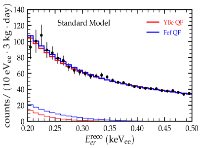
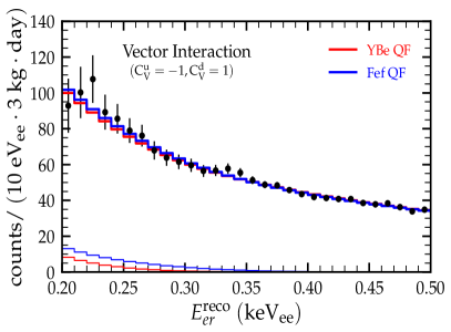
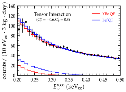
Figure 1: Estimated number of events within the SM and various new physics scenarios considered here, for given benchmark values for the new physics parameters. We also show a comparison of the Rx-ON data reported by the Dresden-II Collaboration. In each panel, the low-lying spectra with thin lines show the predicted signal from “CE$\nu$NS only,” while those with thick lines give the estimated “CE$\nu$NS + fitted background.” Different colors correspond to two QF models.

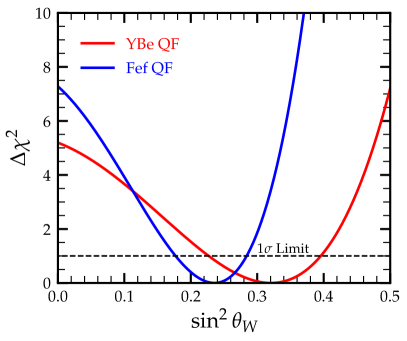
Figure 2: Dresden-II sensitivity on the weak mixing angle, assuming the Fef and YBe QF models.

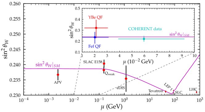
Figure 3: RGE running of the weak mixing angle and experimental measurements across different energies. The inset plot shows our current result obtained from the analysis of Dresden-II data for the different QF models. A comparison with the COHERENT data [3] is also shown.

3.2 Statistical analysis

The statistical analysis in our present work is based on the Gaussian $\chi^{2}$ function [23]

$$\chi^{2}(\overrightarrow{S},a,\upbeta)=\sum_{i=1}^{130}{\left[\frac{(1+a)R^{i}_{\text{CE$\nu$NS}}(\overrightarrow{S})+R^{i}_{\text{bkg}}(\mathbf{\upbeta})-R^{i}_{\text{exp}}}{\sigma^{i}_{\text{exp}}}\right]}^{2}+{\left(\frac{a}{\sigma_{a}}\right)}^{2}+{\left(\frac{\beta_{M/L_{1}}-0.16}{\sigma_{\beta_{M/L_{1}}}}\right)}^{2}\,,$$ (19)

where $R^{i}_{\text{CE$\nu$NS}}$ stands for the theoretically estimated CE$\nu$NS events in the $i$th bin, and $\overrightarrow{S}$ denotes the set of new physics parameters, while $R^{i}_{\text{exp}}$ and $\sigma^{i}_{\text{exp}}$ are the experimental number of events and the corresponding uncertainty in the $i$th bin, all taken from data release [18]. The neutrino flux normalization uncertainty is taken into consideration through the nuisance parameter $a$ with $\sigma_{a}=2$%. Following Ref. [18], the uncertainty of $\beta_{M/L_{1}}$ is taken to be $\sigma_{\beta_{M/L_{1}}}=0.03$, and the prior $0.16$ is assigned. In what follows, for a given parameter of interest from the set $\overrightarrow{S}$, our analysis involves minimization of the $\chi^{2}$ function over each component of $\upbeta$ and $a$.

As a first step, we simulate the event spectra expected at Dresden-II, a procedure which has also served as a validation of our calculation. Figure 1 depicts the efficiency-corrected event rates within and beyond the SM for the different new physics scenarios of interest here. In each panel, we show both the “CE$\nu$NS only” signal and “CE$\nu$NS + fitted background” signal, while the event rates are zoomed in on the recoil energy range $[0.2,0.5]~{}\text{keV}_{ee}$, where CE$\nu$NS has a significant contribution (for the full spectra in the ROI, see Fig. 7 in the Appendix A). Assuming that the experimental data are populated by backgrounds only, we find the best-fit value $\chi^{2}_{\text{min}}=110.69/\text{d.o.f.}$ (d.o.f. stands for the total number of degrees of freedom). On the other hand, by including the predicted SM CE$\nu$NS signal in our analysis, we find the best-fit values $\chi^{2}_{\text{min}}=\{102.66,105.95\}/\text{d.o.f.}$ for {Fef, YBe} QF—i.e., a clear improvement with respect to the background-only hypothesis.

Based on the $\chi^{2}$ function given in Eq. (19) and the Dresden-II data release, we proceed by presenting our results—namely, the parameter determination sensitivities within and beyond the SM for the various physics scenarios described in Sec. 2.

We begin by discussing our new restrictions imposed on the SM weak mixing angle. The corresponding $\Delta\chi^{2}$ profiles of $\sin^{2}{\theta_{W}}$ for the Fef and YBe QFs are shown in Fig. 2. The extracted 1$\sigma$ determinations of the weak mixing angle for our two QFs read

$$\begin{split}\text{Photoneutron QF:}&\text{ }\text{ }\sin^{2}{\theta_{W}}=0.321^{+0.075}_{-0.094}\,,\\ \text{Iron filter QF:}&\text{ }\text{ }\sin^{2}{\theta_{W}}=0.236^{+0.048}_{-0.058}\,.\end{split}$$

One sees that there is a strong dependence on the QF model used. Moreover, our results are in good agreement with those of Ref. [21], though our best-fit point lies closer to the RGE prediction, especially for the case of Fef QF. We can also compare our results with those obtained in Refs. [19, 20], based on the background-subtracted data in Ref. [18]. Exploiting the full Dresden-II data in the present analysis, we find a better agreement with the RGE prediction, but with a higher uncertainty compared to the latter studies. In Fig. 3, we compare our results extracted from the analysis of Dresden-II data with determinations from other probes across a wide range of energies. Let us finally emphasize that even though the Dresden-II data constrain the weak mixing angle with lower significance than the measurement reported by the COHERENT Collaboration [3], it is interesting to notice the complementarity between the two measurements. Clearly, the Dresden-II data fill a gap in the regime of low momentum transfer—e.g., within $10^{-2}-10^{-1}~{}\mathrm{GeV}$.

We now examine the possibility of using the Dresden-II data to extract information on unitarity-violation effects in the neutrino mixing matrix in Eqs. (3) and (4). In Fig. 4 we present the $\Delta\chi^{2}$ profiles of $\alpha_{11}$ and $|\alpha_{12}|$ or $|\alpha_{13}|$, by varying one parameter at a time. As can be seen from Eq.(7), the expected number of events has the same dependence on the off-diagonal NU parameters $|\alpha_{12}|$ and $|\alpha_{13}|$. As a result, they can be constrained by the Dresden-II data with exactly the same sensitivity. We present our results for the two QF models, Fef and YBe. As expected, the Fef-driven results are more constraining, since the pure SM event rate evaluated with the YBe QF is more suppressed, compared to the Fef spectrum. For the case of YBe QF, the predicted event rate contains much fewer events than the spectrum calculated with the Fef QF (see Fig. 1), and hence the NU parameters $|\alpha_{21}|$, $|\alpha_{31}|$ would reach values larger than 1 in order to describe the Dresden-II data, i.e. they would become unphysical.

The 90% C.L. sensitivities on the NU parameters of interest using Dresden-II data are summarized in Table 2. They are compared with those derived from neutrino oscillation global fits [87]. As expected, due to low statistics, large uncertainties on the background model of Dresden-II, as well as poor QF determination, the sensitivities extracted in this work are not competitive with those achievable at the large-scale oscillation experiments. We note, however, that the upcoming sensitivities at the next-generation CE$\nu$NS experiments are rather promising, and they might become competitive with oscillation experiments—see, e.g., Ref. [55].

NU parameter Oscillations [87]    YBe QF    Fef QF $\alpha_{11}$ $>0.98$ $>0.758$ $>0.805$ $\left|\alpha_{12}\right|$ $<10^{-2}$ – $<0.747$ $\left|\alpha_{13}\right|$ $<4.2\times 10^{-2}$ – $<0.747$

Table 2: 90% C.L. sensitivities on NU parameters from the Dresden-II data for YBe and Fef QF. We also give, for comparison, those derived from neutrino oscillation data in Ref. [87].

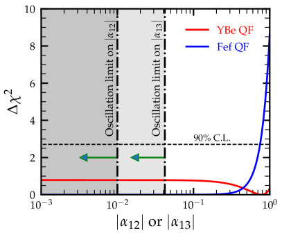
Figure 4: Sensitivity of Dresden-II on NU parameters, $\alpha_{11}$ (left) and $|\alpha_{12}|$ or $|\alpha_{13}|$ (right), for the Fef and YBe QF. Also shown are the corresponding 90% C.L. constraints extracted from neutrino oscillation global fits [87].

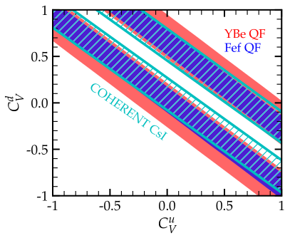
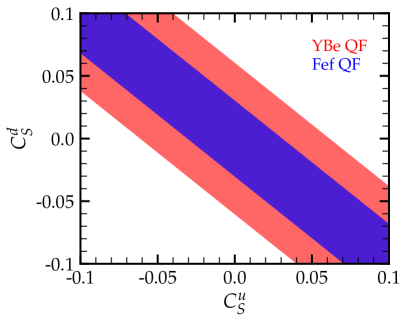
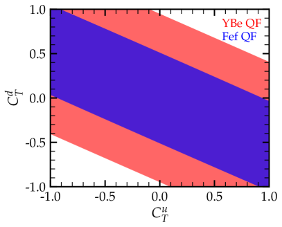
Figure 5: 90% C.L. allowed regions in the vector (top), scalar (lower-left) and tensor (lower-right) NGI parameters ($C_{X}^{u},C_{X}^{d}$). We assume one nonvanishing interaction $X=S,V,T$ at a time and nonuniversal couplings for $u$ and $d$ quarks, for the Fef (in blue) and YBe (in red) quenching factors. For vector interactions, the COHERENT results [3] are superimposed for comparison.

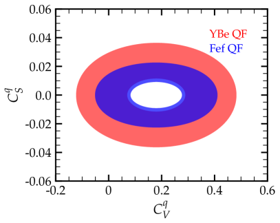
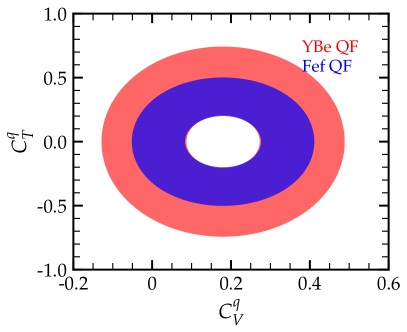
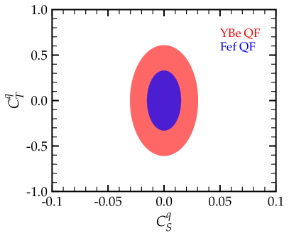
Figure 6: Same as Fig. 5, but for two nonvanishing interactions $X=S,V,T$ at a time, using universal quark couplings.

Now, we finally come to our discussion of the results of our phenomenological analysis of NGIs that includes, as a special case, the conventional NSIs. As discussed in Sec. 2.3, these are expected in low-scale models of neutrino mass generation; see Ref. [25] for a more extended discussion. If NGIs exist, the Dresden-II reactor experiment will be sensitive to a particular combination of the $C_{X}^{q}$ coefficients, specified in Eq. (12). In Fig. 5, we show the corresponding $90\%$ C.L. allowed regions for the NGI coefficients in the $(C_{X}^{u},C_{X}^{d}$) plane. These are obtained by switching on a single interaction $X$ on top of the SM, taking the other two to vanish. As previously, the results are given for both QFs, with the Fef constraints more stringent than the YBe ones. Concerning the NSI case of the vector interaction, our ($C_{V}^{u},C_{V}^{d}$) sensitivity contours (see top graph in Fig. 5) agree very well with those in Refs. [23, 24], and with existing constraints from COHERENT [3]. However, the NGI framework allows us to explore the sensitivity of Dresden-II data on scalar and tensor interactions as well [72]. The corresponding results are given in the lower-left (lower-right) graph of Fig. 5 for scalar (tensor) interactions. As expected, in both cases, there is no destructive interference and the sensitivity contours appear as a single band, unlike the vector case . Interestingly, by comparing the three contours, one can see that the least (most) constrained NGI parameter is the vector (scalar) one. Indeed, we find the best-fit values: $\chi^{2}_{\text{min}}=\{104.53,105.16,104.82\}/\text{d.o.f.}$ using YBe QF and $\{102.59,102.63,102.62\}/\text{d.o.f.}$ using Fef QF for the $(C_{S}^{u},C_{S}^{d})$, $(C_{V}^{u},C_{V}^{d})$, $(C_{T}^{u},C_{T}^{d})$—i.e., the presence of NGIs implies a slight improvement in the fit with respect to the SM result, of no statistical significance.

Within the NGI framework, in principle, all interactions $X=S,V,T$ can be simultaneously active with a total number of six free NGI parameters. Notice that the different kinematic terms corresponding to $X=S,V,T$ interactions in the NGI cross section of Eq.(13) affect the shape of the CE$\nu$NS event rate distribution. In order to reduce the degrees of freedom, while still being able to come out with intuitive results, we will make further reasonable simplifications. First, we assume universal couplings for $u$ and $d$ quarks—i.e., $C_{X}^{u}=C_{X}^{d}=C_{X}^{q}$—thus reducing the degrees of freedom by half without losing information on the spectral shape of the signal. Second, we allow two different interactions to float simultaneously, while the third is set to zero. This way, we can perform a more general analysis, with two different interaction types taken into account simultaneously in our fit. Figure 6 shows the corresponding 90% C.L. sensitivity contours in the $(C_{V}^{q},C_{S}^{q})$, $(C_{V}^{q},C_{T}^{q})$, and $(C_{S}^{q},C_{T}^{q})$ planes for the two QFs. One sees that, in the presence of the vector NGI there is a destructive interference, leaving a “hole” in the $(C_{V}^{q},C_{S}^{q})$, $(C_{V}^{q},C_{T}^{q})$ planes. The best-fit values are: $\chi^{2}_{\text{min}}=\{103.81,104.39,104.54\}/\text{d.o.f.}$ using YBe QF, and $\{102.01,102.05,102.59\}/\text{d.o.f.}$ using Fef QF for $(C_{V}^{q},C_{S}^{q})$, $(C_{V}^{q},C_{T}^{q})$, and $(C_{S}^{q},C_{T}^{q})$, respectively. Thus, we conclude that a combined analysis with two nonzero NGIs at a time leads to a slight improvement in the fit compared to the pure SM case, or a single nonvanishing NGI type.

4 Conclusions

We have analyzed the new data released by the Dresden-II Collaboration which reported, for the first time, a suggestive evidence of CE$\nu$NS observation using reactor antineutrinos. We performed a careful statistical analysis of the event spectral distributions, estimating the expected background sources according to the prescription given by the Dresden-II Collaboration: see Fig. 1. Using the available data, we explored different physics schemes within and beyond the SM. We first examined the new determination of the weak mixing angle in the low-energy regime, given in Fig. 2. Although our Dresden-II determination is not as competitive as the existing one from the COHERENT data, the best-fit value is in better agreement with the theoretical prediction from RGE extrapolations (Fig. 3). However, one should note that the best-fit value differs dramatically for the two QF models we have adopted.

Concerning new physics scenarios, we focused on two different examples namely, the potential violation of unitarity in the neutrino mixing matrix, as well as the presence of new neutrino interactions due to heavy mediators. As seen in Fig. 4, current Dresden-II data do not have sufficient statistics to place a competitive constraint on unitarity violation parameters. However, short baseline reactor CE$\nu$NS experiments may provide a promising unitarity violation probe in the long run. Finally, we examined the Dresden-II limits on the most general neutrino interactions due to heavy mediators, given in Figs. 5 and 6. These are competitive with those obtained at COHERENT for the case of vector interaction. We have also obtained the corresponding sensitivities for scalar and tensor CE$\nu$NS interactions. Though not significant, their interplay may improve the description of the Dresden-II data.

Appendix A Details of the data fitting

In this section, we briefly discuss the details of the determination of the expected background events for the Dresden-II data used in this work. As already mentioned in Sec. 3, the background model characterized by seven free parameters is reported in Ref. [18]. Note also that every analysis requires simultaneous fitting of the free background parameters in addition to the physics parameters of interest within or beyond the SM. Hence, in this work we paid special attention in adopting a careful fitting procedure. In Fig. 7, we demonstrate the SM “CE$\nu$NS only” signal and the “CE$\nu$NS + fitted background” signal in the full ROI of the Dresden-II experiment. In contrast to Refs. [23, 21], which employed a differential spectrum, here we make different background assumptions. Namely, the background model of Eq.(18) is taken to be an integrated spectrum for which the parameters $N_{\text{epith}}$, $A_{\text{epith}}$, and $A_{L_{1},L_{2},L_{M}}$ are given in units of $\mathrm{counts/\left(10~{}eV_{ee}\cdot 3~{}kg\cdot day\right)}$, in line with the approach followed by the Dresden-II Collaboration. Although this may not lead to significant differences, we stress that in our analysis the background parameters are varied within their allowed ranges, unspecified in Refs. [23, 21]. The most notable difference with those works is that here the exponential decay function characterizing the epithermal neutron background component is taken to be centered at $E_{\text{epith}}=0.2~{}\mathrm{keV_{ee}}$ instead of zero. The allowed ranges and the best-fit values of free background parameters are listed in Table 3. For each case, the best-fit values we obtain are in agreement with the corresponding $1~{}\sigma$ limit reported in the ancillary file of Ref. [18].

Background Parameters ($\upbeta$)	Allowed range	YBe QF	Fef QF
$N_{\text{epith}}$	$[0,~{}25]$	$14.082$	$13.779$
$A_{\text{epith}}$	$[0,~{}150]$	$66.505$	$62.947$
$\tau_{\text{epith}}\text{ (keV)}$	$[0,~{}2]$	$0.249$	$0.262$
$A_{L_{1}}$	$[70,~{}250]$	$84.577$	$84.63$
$E_{L_{1}}\text{ (keV)}$	$[1.2,~{}1.4]$	$1.29228$	$1.29237$
$\sigma_{L_{1}}\text{ (keV)}$	$[0.04,~{}0.1]$	$0.0694$	$0.06963$
$\beta_{M/L_{1}}$	$[0,~{}0.3]$	$0.17$	$0.158$
Fitted events (SM $+$ Background)		$5080.29$	$5103.4$
$\chi^{2}_{\text{min}}$		$105.95/\text{d.o.f.}$	$102.66/\text{d.o.f.}$

Table 3: Best-fit values for the background model parameters and total number of signal events. The values of $N_{\text{epith}}$, $A_{\text{epith}}$, $A_{L_{1}}$, as well as the fitted events are all given in units of $\mathrm{[counts/\left(10~{}eV_{ee}\cdot 3~{}kg\cdot day\right)]}$.

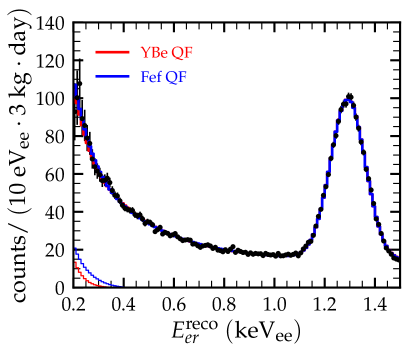
Figure 7: SM “CE$\nu$NS only” (thin lines) and “CE$\nu$NS + fitted background” (thick lines) signal in the full ROI of the Dresden-II measurement.

References

- [1] D. Z. Freedman, “Coherent Neutrino Nucleus Scattering as a Probe of the Weak Neutral Current,” Phys. Rev. D 9 (1974) 1389–1392.
- [2] COHERENT Collaboration, D. Akimov et al., “Observation of Coherent Elastic Neutrino-Nucleus Scattering,” Science 357 no. 6356, (2017) 1123–1126, arXiv:1708.01294 [nucl-ex].
- [3] COHERENT Collaboration, D. Akimov et al., “Measurement of the Coherent Elastic Neutrino-Nucleus Scattering Cross Section on CsI by COHERENT,” Phys. Rev. Lett. 129 no. 8, (2022) 081801, arXiv:2110.07730 [hep-ex].
- [4] COHERENT Collaboration, D. Akimov et al., “First Measurement of Coherent Elastic Neutrino-Nucleus Scattering on Argon,” Phys. Rev. Lett. 126 no. 1, (2021) 012002, arXiv:2003.10630 [nucl-ex].
- [5] CONNIE Collaboration, A. Aguilar-Arevalo et al., “Search for coherent elastic neutrino-nucleus scattering at a nuclear reactor with CONNIE 2019 data,” JHEP 05 (2022) 017, arXiv:2110.13033 [hep-ex].
- [6] CONUS Collaboration, H. Bonet et al., “Constraints on Elastic Neutrino Nucleus Scattering in the Fully Coherent Regime from the CONUS Experiment,” Phys. Rev. Lett. 126 no. 4, (2021) 041804, arXiv:2011.00210 [hep-ex].
- [7] CONUS Collaboration, H. Bonet et al., “Novel constraints on neutrino physics beyond the standard model from the CONUS experiment,” JHEP 05 (2022) 085, arXiv:2110.02174 [hep-ph].
- [8] GeN Collaboration, I. Alekseev et al., “First results of the experiment on coherent elastic neutrino-nucleus scattering,” Phys. Rev. D 106 no. 5, (2022) L051101, arXiv:2205.04305 [nucl-ex].
- [9] MINER Collaboration, G. Agnolet et al., “Background Studies for the MINER Coherent Neutrino Scattering Reactor Experiment,” Nucl. Instrum. Meth. A 853 (2017) 53–60, arXiv:1609.02066 [physics.ins-det].
- [10] J. Billard et al., “Coherent Neutrino Scattering with Low Temperature Bolometers at Chooz Reactor Complex,” J. Phys. G 44 no. 10, (2017) 105101, arXiv:1612.09035 [physics.ins-det].
- [11] R. Strauss et al., “The -cleus experiment: A gram-scale fiducial-volume cryogenic detector for the first detection of coherent neutrino-nucleus scattering,” Eur. Phys. J. C 77 (2017) 506, arXiv:1704.04320 [physics.ins-det].
- [12] H. T.-K. Wong, “Taiwan EXperiment On NeutrinO — History and Prospects,” The Universe 3 no. 4, (2015) 22–37, arXiv:1608.00306 [hep-ex].
- [13] G. Fernandez-Moroni, P. A. N. Machado, I. Martinez-Soler, Y. F. Perez-Gonzalez, D. Rodrigues, and S. Rosauro-Alcaraz, “The physics potential of a reactor neutrino experiment with Skipper CCDs: Measuring the weak mixing angle,” JHEP 03 (2021) 186, arXiv:2009.10741 [hep-ph].
- [14] SBC, CENS Theory Group at IF-UNAM Collaboration, L. J. Flores et al., “Physics reach of a low threshold scintillating argon bubble chamber in coherent elastic neutrino-nucleus scattering reactor experiments,” Phys. Rev. D 103 no. 9, (2021) L091301, arXiv:2101.08785 [hep-ex].
- [15] D. Baxter et al., “Coherent Elastic Neutrino-Nucleus Scattering at the European Spallation Source,” JHEP 02 (2020) 123, arXiv:1911.00762 [physics.ins-det].
- [16] CCM Collaboration, A. A. Aguilar-Arevalo et al., “First Leptophobic Dark Matter Search from the Coherent–CAPTAIN-Mills Liquid Argon Detector,” Phys. Rev. Lett. 129 no. 2, (2022) 021801, arXiv:2109.14146 [hep-ex].
- [17] J. Colaresi, J. I. Collar, T. W. Hossbach, A. R. L. Kavner, C. M. Lewis, A. E. Robinson, and K. M. Yocum, “First results from a search for coherent elastic neutrino-nucleus scattering at a reactor site,” Phys. Rev. D 104 no. 7, (2021) 072003, arXiv:2108.02880 [hep-ex].
- [18] J. Colaresi, J. I. Collar, T. W. Hossbach, C. M. Lewis, and K. M. Yocum, “Measurement of Coherent Elastic Neutrino-Nucleus Scattering from Reactor Antineutrinos,” Phys. Rev. Lett. 129 no. 21, (2022) 211802, arXiv:2202.09672 [hep-ex].
- [19] D. Aristizabal Sierra, V. De Romeri, and D. K. Papoulias, “Consequences of the Dresden-II reactor data for the weak mixing angle and new physics,” JHEP 09 (2022) 076, arXiv:2203.02414 [hep-ph].
- [20] A. N. Khan, “ and neutrino electromagnetic interactions in CENS with different quenching factors,” arXiv:2203.08892 [hep-ph].
- [21] M. Atzori Corona, M. Cadeddu, N. Cargioli, F. Dordei, C. Giunti, Y. F. Li, C. A. Ternes, and Y. Y. Zhang, “Impact of the Dresden-II and COHERENT neutrino scattering data on neutrino electromagnetic properties and electroweak physics,” JHEP 09 (2022) 164, arXiv:2205.09484 [hep-ph].
- [22] J. Liao, H. Liu, and D. Marfatia, “Implications of the first evidence for coherent elastic scattering of reactor neutrinos,” Phys. Rev. D 106 no. 3, (2022) L031702, arXiv:2202.10622 [hep-ph].
- [23] P. Coloma, I. Esteban, M. C. Gonzalez-Garcia, L. Larizgoitia, F. Monrabal, and S. Palomares-Ruiz, “Bounds on new physics with data of the Dresden-II reactor experiment and COHERENT,” JHEP 05 (2022) 037, arXiv:2202.10829 [hep-ph].
- [24] P. B. Denton and J. Gehrlein, “New constraints on the dark side of non-standard interactions from reactor neutrino scattering data,” Phys. Rev. D 106 no. 1, (2022) 015022, arXiv:2204.09060 [hep-ph].
- [25] S. M. Boucenna, S. Morisi, and J. W. F. Valle, “The low-scale approach to neutrino masses,” Adv.High Energy Phys. 2014 (2014) 831598, arXiv:1404.3751 [hep-ph].
- [26] R. N. Mohapatra and J. W. F. Valle, “Neutrino Mass and Baryon Number Nonconservation in Superstring Models,” Phys. Rev. D 34 (1986) 1642.
- [27] M. Gonzalez-Garcia and J. W. F. Valle, “Fast Decaying Neutrinos and Observable Flavor Violation in a New Class of Majoron Models,” Phys.Lett.B 216 (1989) 360–366.
- [28] E. K. Akhmedov et al., “Left-right symmetry breaking in NJL approach,” Phys.Lett.B 368 (1996) 270–280, arXiv:hep-ph/9507275 [hep-ph].
- [29] E. K. Akhmedov et al., “Dynamical left-right symmetry breaking,” Phys.Rev.D 53 (1996) 2752–2780, arXiv:hep-ph/9509255 [hep-ph].
- [30] M. Malinsky, J. Romao, and J. W. F. Valle, “Novel supersymmetric SO(10) seesaw mechanism,” Phys.Rev.Lett. 95 (2005) 161801, arXiv:hep-ph/0506296 [hep-ph].
- [31] M. Dittmar, A. Santamaria, M. Gonzalez-Garcia, and J. W. F. Valle, “Production Mechanisms and Signatures of Isosinglet Neutral Heavy Leptons in Decays,” Nucl.Phys.B 332 (1990) 1–19.
- [32] M. Gonzalez-Garcia, A. Santamaria, and J. W. F. Valle, “Isosinglet Neutral Heavy Lepton Production in Decays and Neutrino Mass,” Nucl.Phys.B 342 (1990) 108–126.
- [33] J. Aguilar-Saavedra, F. Deppisch, O. Kittel, and J. W. F. Valle, “Flavour in heavy neutrino searches at the LHC,” Phys.Rev.D 85 (2012) 091301, arXiv:1203.5998 [hep-ph].
- [34] S. Das, F. Deppisch, O. Kittel, and J. W. F. Valle, “Heavy Neutrinos and Lepton Flavour Violation in Left-Right Symmetric Models at the LHC,” Phys.Rev.D 86 (2012) 055006, arXiv:1206.0256 [hep-ph].
- [35] F. F. Deppisch, N. Desai, and J. W. F. Valle, “Is charged lepton flavor violation a high energy phenomenon?,” Phys.Rev.D 89 (2014) 051302, arXiv:1308.6789 [hep-ph].
- [36] ATLAS Collaboration, G. Aad et al., “Search for heavy neutral leptons in decays of bosons produced in 13 TeV collisions using prompt and displaced signatures with the ATLAS detector,” JHEP 10 (2019) 265, arXiv:1905.09787 [hep-ex].
- [37] CMS Collaboration, A. M. Sirunyan et al., “Search for heavy neutral leptons in events with three charged leptons in proton-proton collisions at 13 TeV,” Phys.Rev.Lett. 120 (2018) 221801, arXiv:1802.02965 [hep-ex].
- [38] CMS Collaboration, A. Tumasyan et al., “Inclusive nonresonant multilepton probes of new phenomena at s=13 TeV,” Phys.Rev.D 105 no. 11, (2022) 112007, arXiv:2202.08676 [hep-ex].
- [39] M. Drewes and J. Hajer, “Heavy Neutrinos in displaced vertex searches at the LHC and HL-LHC,” JHEP 02 (2020) 070, arXiv:1903.06100 [hep-ph].
- [40] A. M. Abdullahi et al., “The Present and Future Status of Heavy Neutral Leptons,” in 2022 Snowmass Summer Study. 3, 2022. arXiv:2203.08039 [hep-ph].
- [41] D. K. Papoulias, R. Sahu, T. S. Kosmas, V. K. B. Kota, and B. Nayak, “Novel neutrino-floor and dark matter searches with deformed shell model calculations,” Adv. High Energy Phys. 2018 (2018) 6031362, arXiv:1804.11319 [hep-ph].
- [42] A. Drukier and L. Stodolsky, “Principles and Applications of a Neutral Current Detector for Neutrino Physics and Astronomy,” Phys. Rev. D 30 (1984) 2295.
- [43] J. Barranco, O. G. Miranda, and T. I. Rashba, “Probing new physics with coherent neutrino scattering off nuclei,” JHEP 12 (2005) 021, arXiv:hep-ph/0508299.
- [44] D. K. Papoulias, T. S. Kosmas, and Y. Kuno, “Recent probes of standard and non-standard neutrino physics with nuclei,” Front. in Phys. 7 (2019) 191, arXiv:1911.00916 [hep-ph].
- [45] D. K. Papoulias and T. S. Kosmas, “Standard and Nonstandard Neutrino-Nucleus Reactions Cross Sections and Event Rates to Neutrino Detection Experiments,” Adv. High Energy Phys. 2015 (2015) 763648, arXiv:1502.02928 [nucl-th].
- [46] S. Weinberg, “A Model of Leptons,” Phys. Rev. Lett. 19 (1967) 1264–1266.
- [47] Particle Data Group Collaboration, R. L. Workman, “Review of Particle Physics,” PTEP 2022 (2022) 083C01.
- [48] J. Erler and M. Schott, “Electroweak Precision Tests of the Standard Model after the Discovery of the Higgs Boson,” Prog. Part. Nucl. Phys. 106 (2019) 68–119, arXiv:1902.05142 [hep-ph].
- [49] M. Cadeddu, N. Cargioli, F. Dordei, C. Giunti, Y. F. Li, E. Picciau, C. A. Ternes, and Y. Y. Zhang, “New insights into nuclear physics and weak mixing angle using electroweak probes,” Phys. Rev. C 104 no. 6, (2021) 065502, arXiv:2102.06153 [hep-ph].
- [50] C. S. Wood, S. C. Bennett, D. Cho, B. P. Masterson, J. L. Roberts, C. E. Tanner, and C. E. Wieman, “Measurement of parity nonconservation and an anapole moment in cesium,” Science 275 (1997) 1759–1763.
- [51] J. Guena, M. Lintz, and M. A. Bouchiat, “Measurement of the parity violating 6S-7S transition amplitude in cesium achieved within 2 x 10(-13) atomic-unit accuracy by stimulated-emission detection,” Phys. Rev. A 71 (2005) 042108, arXiv:physics/0412017.
- [52] J. Schechter and J. W. F. Valle, “Neutrino Masses in SU(2) x U(1) Theories,” Phys. Rev. D 22 (1980) 2227.
- [53] J. Schechter and J. W. F. Valle, “Neutrino Decay and Spontaneous Violation of Lepton Number,” Phys.Rev.D 25 (1982) 774.
- [54] F. J. Escrihuela, D. V. Forero, O. G. Miranda, M. Tortola, and J. W. F. Valle, “On the description of nonunitary neutrino mixing,” Phys. Rev. D 92 no. 5, (2015) 053009, arXiv:1503.08879 [hep-ph]. [Erratum: Phys.Rev.D 93, 119905 (2016)].
- [55] O. G. Miranda, D. K. Papoulias, O. Sanders, M. Tórtola, and J. W. F. Valle, “Future CEvNS experiments as probes of lepton unitarity and light-sterile neutrinos,” Phys. Rev. D 102 (2020) 113014, arXiv:2008.02759 [hep-ph].
- [56] E. Alfonso-Pita, L. J. Flores, E. Peinado, and E. Vázquez-Jáuregui, “New physics searches in a low threshold scintillating argon bubble chamber measuring coherent elastic neutrino-nucleus scattering in reactors,” Phys. Rev. D 105 no. 11, (2022) 113005, arXiv:2203.05982 [hep-ph].
- [57] L. Wolfenstein, “Neutrino Oscillations in Matter,” Phys.Rev.D 17 (1978) 2369–2374.
- [58] J. W. F. Valle, “Resonant Oscillations of Massless Neutrinos in Matter,” Phys.Lett.B 199 (1987) 432–436.
- [59] T. D. Lee and C.-N. Yang, “Question of Parity Conservation in Weak Interactions,” Phys. Rev. 104 (1956) 254–258.
- [60] T. Ohlsson, “Status of non-standard neutrino interactions,” Rept. Prog. Phys. 76 (2013) 044201, arXiv:1209.2710 [hep-ph].
- [61] Y. Farzan and M. Tortola, “Neutrino oscillations and Non-Standard Interactions,” Front. in Phys. 6 (2018) 10, arXiv:1710.09360 [hep-ph].
- [62] J. Billard, J. Johnston, and B. J. Kavanagh, “Prospects for exploring New Physics in Coherent Elastic Neutrino-Nucleus Scattering,” JCAP 11 (2018) 016, arXiv:1805.01798 [hep-ph].
- [63] D. K. Papoulias and T. S. Kosmas, “COHERENT constraints to conventional and exotic neutrino physics,” Phys. Rev. D 97 no. 3, (2018) 033003, arXiv:1711.09773 [hep-ph].
- [64] D. K. Papoulias, “COHERENT constraints after the COHERENT-2020 quenching factor measurement,” Phys.Rev. D102 (2020) 113004, arXiv:1907.11644 [hep-ph].
- [65] O. Miranda, D. Papoulias, G. Sanchez Garcia, O. Sanders, M. Tórtola, and J. W. F. Valle, “Implications of the first detection of coherent elastic neutrino-nucleus scattering (CEvNS) with Liquid Argon,” JHEP 2005 (2020) 130, arXiv:2003.12050 [hep-ph].
- [66] C. Giunti, “General COHERENT constraints on neutrino nonstandard interactions,” Phys.Rev. D101 (2020) 035039, arXiv:1909.00466 [hep-ph].
- [67] A. N. Khan, D. W. McKay, and W. Rodejohann, “CP-violating and charged current neutrino nonstandard interactions in CENS,” Phys.Rev.D 104 (2021) 015019, arXiv:2104.00425 [hep-ph].
- [68] B. Dutta, R. F. Lang, S. Liao, S. Sinha, L. Strigari, and A. Thompson, “A global analysis strategy to resolve neutrino NSI degeneracies with scattering and oscillation data,” JHEP 2009 (2020) 106, arXiv:2002.03066 [hep-ph].
- [69] B. Canas, E. Garces, O. Miranda, A. Parada, and G. Sanchez Garcia, “Interplay between nonstandard and nuclear constraints in coherent elastic neutrino-nucleus scattering experiments,” Phys.Rev. D101 (2020) 035012, arXiv:1911.09831 [hep-ph].
- [70] P. Coloma, I. Esteban, M. Gonzalez-Garcia, and M. Maltoni, “Improved global fit to Non-Standard neutrino Interactions using COHERENT energy and timing data,” JHEP 2002 (2020) 023, arXiv:1911.09109 [hep-ph].
- [71] S. S. Chatterjee, S. Lavignac, O. Miranda, and G. Sanchez Garcia, “Constraining Non-Standard Interactions with Coherent Elastic Neutrino-Nucleus Scattering at the European Spallation Source,” arXiv:2208.11771 [hep-ph].
- [72] M. Lindner, W. Rodejohann, and X.-J. Xu, “Coherent Neutrino-Nucleus Scattering and new Neutrino Interactions,” JHEP 03 (2017) 097, arXiv:1612.04150 [hep-ph].
- [73] E. E. Jenkins, A. V. Manohar, and P. Stoffer, “Low-Energy Effective Field Theory below the Electroweak Scale: Operators and Matching,” JHEP 03 (2018) 016, arXiv:1709.04486 [hep-ph].
- [74] D. Aristizabal Sierra, V. De Romeri, and N. Rojas, “COHERENT analysis of neutrino generalized interactions,” Phys. Rev. D 98 (2018) 075018, arXiv:1806.07424 [hep-ph].
- [75] J. B. Dent, L. M. Krauss, J. L. Newstead, and S. Sabharwal, “General analysis of direct dark matter detection: From microphysics to observational signatures,” Phys. Rev. D 92 no. 6, (2015) 063515, arXiv:1505.03117 [hep-ph].
- [76] M. Cirelli, E. Del Nobile, and P. Panci, “Tools for model-independent bounds in direct dark matter searches,” JCAP 10 (2013) 019, arXiv:1307.5955 [hep-ph].
- [77] D. Aristizabal Sierra, J. Liao, and D. Marfatia, “Impact of form factor uncertainties on interpretations of coherent elastic neutrino-nucleus scattering data,” JHEP 06 (2019) 141, arXiv:1902.07398 [hep-ph].
- [78] L. J. Flores, N. Nath, and E. Peinado, “CENS as a probe of flavored generalized neutrino interactions,” Phys. Rev. D 105 no. 5, (2022) 055010, arXiv:2112.05103 [hep-ph].
- [79] CONNIE Collaboration, A. Aguilar-Arevalo et al., “Search for light mediators in the low-energy data of the CONNIE reactor neutrino experiment,” JHEP 04 (2020) 054, arXiv:1910.04951 [hep-ex].
- [80] S. Antman, D. Landis, and R. Pehl, “Measurements of the fano factor and the energy per hole-electron pair in germanium,” Nuclear Instruments and Methods 40 no. 2, (1966) 272–276. https://www.sciencedirect.com/science/article/pii/0029554X66903867.
- [81] W. Z. Wei, L. Wang, and D. M. Mei, “Average energy expended per e-h pair for germanium-based dark matter experiments,” JINST 12 no. 04, (2017) P04022, arXiv:1602.08005 [physics.ins-det].
- [82] M. Berglund and M. E. Wieser, “Isotopic compositions of the elements 2009 (iupac technical report),” Pure and Applied Chemistry 83 no. 2, (2011) 397–410.
- [83] B. J. Scholz, A. E. Chavarria, J. I. Collar, P. Privitera, and A. E. Robinson, “Measurement of the low-energy quenching factor in germanium using an 88Y/Be photoneutron source,” Phys. Rev. D 94 no. 12, (2016) 122003, arXiv:1608.03588 [physics.ins-det].
- [84] J. I. Collar, A. R. L. Kavner, and C. M. Lewis, “Germanium response to sub-keV nuclear recoils: a multipronged experimental characterization,” Phys. Rev. D 103 no. 12, (2021) 122003, arXiv:2102.10089 [nucl-ex].
- [85] E. Schoenfeld, “Calculation of fractional electron capture probabilities,” Applied Radiation and Isotopes 49 no. 9-11, (Sep 1998) 1353–1357. http://inis.iaea.org/search/search.aspx?orig_q=RN:34013588. Nuclear physics and radiation physics.
- [86] SuperCDMS Collaboration, R. Agnese et al., “New Results from the Search for Low-Mass Weakly Interacting Massive Particles with the CDMS Low Ionization Threshold Experiment,” Phys. Rev. Lett. 116 no. 7, (2016) 071301, arXiv:1509.02448 [astro-ph.CO].
- [87] F. J. Escrihuela et al., “Probing CP violation with non-unitary mixing in long-baseline neutrino oscillation experiments: DUNE as a case study,” New J. Phys. 19 no. 9, (2017) 093005, arXiv:1612.07377 [hep-ph].