Bounds for rotating convection at infinite Prandtl number from semidefinite programs

Abstract

Bounds for the poloidal and toroidal kinetic energies and the heat transport are computed numerically for rotating convection at infinite Prandtl number with both no slip and stress free boundaries. The constraints invoked in this computation are linear or quadratic in the problem variables and lead to the formulation of a semidefinite program. The bounds behave as a function of Rayleigh number at fixed Taylor number qualitatively in the same way as the quantities being bounded. The bounds are zero for Rayleigh numbers smaller than the critical Rayleigh number for the onset of convection, they increase rapidly with Rayleigh number for Rayleigh numbers just above onset, and increase more slowly at large Rayleigh numbers. If the dependencies on Rayleigh number are approximated by power laws, one obtains larger exponents from bounds on the Nusselt number for Rayleigh numbers just above onset than from the actual Nusselt number dependence known for large but finite Prandtl number. The wavelength of the linearly unstable mode at the onset of convection appears as a relevant length scale in the bounds.

I Introduction

The optimum theory of turbulence attempts to replace the exact computation of time averaged global quantities, such as the heat transfer across a convecting layer, by a simpler calculation at the price of obtaining only upper bounds to the quantities of interest. The method most frequently used for this purpose is the background field method Hopf (1941); Doering and Constantin (1992, 1996); Fantuzzi, Arslan, and Wynn (2022), which is more convenient to use but which ultimately produces the same results as another method based on refs. Malkus, 1956; Howard, 1963; Busse, 1969, at least for the convection problem Kerswell (2001). Both classes of methods do not make use of the full Navier-Stokes equation but use relations derived from integrals of this equation, such as the energy budget. As a consequence, a major disadvantage of these methods applied to convection flows is that they are insensitive to the presence of the Coriolis term in the momentum equation. Rotational effects appear in the bounds derived from straightforward optimum theory of convection only for reduced sets of equations Grooms and Whitehead (2014); Pachev et al. (2020), the simplest representative of which is the model of the infinite Prandtl number.

Rotating convection is a problem with many applications in geophysics and astrophysics. In this context, convection at large Prandtl numbers in particular also plays a role. Solutal convection in the oceans or in planetary cores Jones (2015) is characterized by Prandtl numbers around $10^{3}$ or $10^{4}$. It is not obvious if, or under which conditions, rotating convection with Prandtl numbers this large behaves the same as convection in a fluid of infinite Prandtl number. However, these applications motivate the study of convection at infinite Prandtl number as a simple limiting case. In addition, it was recently shown Tilgner (2022) how bounds derived for infinite Prandtl number convection can be used as a starting point for the computation of bounds for arbitrary Prandtl number. This calculation can be summarized as a background field method with a background field for velocity which is not fixed in advance and time independent, but which instead is the solution of the momentum equation for infinite Prandtl number. The bounds derived in this manner for general Prandtl number cannot be lower than the bounds for infinite Prandtl number. It is therefore interesting to explore numerically which are the best possible bounds derivable at infinite Prandtl number from the constraints used in optimum theory of turbulence as we presently know it.

The known bounds derived by analytical means Doering and Constantin (2001); Constantin, Hallstrom, and Putkaradze (1999); Tilgner (2022) for the heat transfer in rotating infinite Prandtl number convection are too loose to be satisfactory. While these bounds qualitatively reproduce a reduction of the heat transport by rotation, they do not restrict the advective heat transfer to zero for Rayleigh numbers below the critical Rayleigh number computed from linear stability analysis.

A numerical computation of upper bounds for heat transfer in rotating convection at infinite Prandtl number with stress free boundaries previously appeared in ref. Vitanov, 2003. The parameter range covered in that study is too small to allow us to really judge the performance of the bounds by comparing them with experimental data. We also know from the non rotating problem that the optimum theory for infinite Prandtl number behaves very differently for stress free and no slip boundaries Plasting and Ierley (2005); Ierley, Kerswell, and Plasting (2006), and the boundary conditions relevant for experiments are no slip rather than stress free boundaries. Finally, ref. Vitanov, 2003 did not compute bounds on energies.

There are thus several motivations to revisit the problem of determining numerically the optimal bounds for rotating convection at infinite Prandtl number. The computation presented here makes use of the same constraints as previous work. These constraints only include linear and quadratic terms. This problem can be cast in the form of a semidefinite program (SDP). Numerical techniques of SDP have already been applied to convection problems Tilgner (2017, 2019) and they promise to be more generally applicable to bounding hydrodynamic quantities Chernyshenko et al. (2014); Fantuzzi, Arslan, and Wynn (2022). The SDP implemented for rotating convection at infinite Prandtl number is explained in the next section, and the results are presented in section 3.

II The Semidefinite Program

We consider a plane layer infinitely extended in the $x$ and $y$ directions and of thickness $h$ with bounding planes perpendicular to the $z$ axis in a frame of reference rotating with angular velocity $\Omega$ about the $z$ axis. The gravitational acceleration acts in the direction of negative $z$. The layer is filled with fluid of density $\rho$, kinematic viscosity $\nu$, thermal diffusivity $\kappa$, and thermal expansion coefficient $\alpha$. Top and bottom boundaries are held at the fixed temperatures $T_{\mathrm{top}}$ and $T_{\mathrm{top}}+\Delta T$, respectively. Within the Boussinesq approximation, there are in general three control parameters: the Prandtl, Rayleigh and Taylor numbers $\mathrm{Pr}$, $\mathrm{Ra}$ and $\mathrm{Ta}$ defined as

$$\mathrm{Pr}=\frac{\nu}{\kappa}~{}~{}~{},~{}~{}~{}\mathrm{Ra}=\frac{g\alpha\Delta Th^{3}}{\kappa\nu}~{}~{}~{},~{}~{}~{}\mathrm{Ta}=\frac{4\Omega^{2}h^{4}}{\nu^{2}}.$$ (1)

Here, we immediately specialize to the limit of infinite $\mathrm{Pr}$ in which case the equations of evolution may be written as follows in terms of the non dimensional fields of velocity $\bm{v}(\bm{r},t)$, pressure $p(\bm{r},t)$ and temperature deviation from the conductive temperature profile $\theta(\bm{r},t)$ where $\theta(\bm{r},t)=T(\bm{r},t)-1+z$ with $T(\bm{r},t)$ being the temperature:

$$\sqrt{\mathrm{Ta}}\bm{\hat{z}}\times\bm{v} = -\nabla p+\mathrm{Ra}\theta\bm{\hat{z}}+\nabla^{2}\bm{v}$$ (2)

$$\partial_{t}\theta+\bm{v}\cdot\nabla\theta-v_{z} = \nabla^{2}\theta$$ (3)

$$\nabla\cdot\bm{v} = 0$$ (4)

$\bm{\hat{z}}$ denotes the unit vector in $z$ direction. The conditions at the boundaries $z=0$ and $z=1$ on the temperature imply that $\theta=0$ there. Both stress free and no slip conditions will be investigated. At stress free boundaries, $\partial_{z}v_{x}=\partial_{z}v_{y}=v_{z}=0$, whereas $\bm{v}=0$ on no slip boundaries. Periodic boundary conditions are assumed in the horizontal directions with arbitrary periodicity lengths.

We now decompose $\bm{v}$ into poloidal and toroidal scalars $\phi$ and $\psi$ such that $\bm{v}=\nabla\times\nabla\times(\phi\bm{\hat{z}})+\nabla\times(\psi\bm{\hat{z}})$ which automatically fulfills $\nabla\cdot\bm{v}=0$. An additional term with a mean flow is not necessary at infinite Prandtl number Tilgner (2022). The $z$ component of the curl and the $z$ component of the curl of the curl of eq. (2) yield the equations of evolution for $\phi$ and $\psi$,

$$\sqrt{\mathrm{Ta}}\partial_{z}\Delta_{2}\psi = \nabla^{2}\nabla^{2}\Delta_{2}\phi-\mathrm{Ra}\Delta_{2}\theta$$ (5)

$$-\sqrt{\mathrm{Ta}}\partial_{z}\Delta_{2}\phi = \nabla^{2}\Delta_{2}\psi$$ (6)

with $\Delta_{2}=\partial^{2}_{x}+\partial^{2}_{y}$. The boundary conditions become $\phi=\partial^{2}_{z}\phi=\partial_{z}\psi=0$ for stress free boundaries and $\phi=\partial_{z}\phi=\psi=0$ for no slip boundaries.

The eqs. (5) and (6) determine $\phi$ and $\psi$, and hence $\bm{v}$, in dependence of $\theta$. The equations of evolution (2-4) therefore reduce to the single equation (3) in which $\bm{v}$ ultimately is some function of $\theta$. Since there is no closed expression for this function, we keep the variables $\phi$, $\psi$ and $\bm{v}$ in subsequent formulae bearing in mind that they are nothing but functions of $\theta$.

We next define averages over space of a function $f(\bm{r})$ and over time of a function $g(t)$ with the symbols

$$\overline{f(t)}=\lim_{\tau\rightarrow\infty}\frac{1}{\tau}\int_{0}^{\tau}f(t)dt~{}~{}~{},~{}~{}~{}\langle g(\bm{r})\rangle=\frac{1}{V}\int g(\bm{r})dV$$ (7)

where $V$ is the volume of a periodicity volume. The product of eq. (3) with $\theta$ followed by a volume average leads in this notation to

$$\partial_{t}\langle\frac{1}{2}\theta^{2}\rangle=\langle v_{z}\theta\rangle-\langle|\nabla\theta|^{2}\rangle.$$ (8)

The quantities for which we will seek bounds in this paper are the time and volume averaged heat transport $\langle\overline{v_{z}\theta}\rangle$, the poloidal energy

$$E_{\mathrm{pol}}=\langle\frac{1}{2}\overline{|\nabla\times\nabla\times(\phi\bm{\hat{z}})|^{2}}\rangle$$ (9)

and the toroidal energy

$$E_{\mathrm{tor}}=\langle\frac{1}{2}\overline{|\nabla\times(\psi\bm{\hat{z}})|^{2}}\rangle.$$ (10)

It only makes sense to ask for bounds on energy in convection with stress free boundaries if one specifies a certain frame of reference because any solution to the equations of evolution may be transformed to another solution with stress free boundary conditions simply by changing to another frame of reference moving at an arbitrarily large horizontal translation velocity. We adopt the same convention as in Ref. Tilgner, 2022 and select the frame of reference in which total momentum is zero.

The method to find these bounds is exactly the same as in Ref. Tilgner, 2017. The only difference in the numerical implementation is that in the non rotating problem of Ref. Tilgner, 2017, the toroidal scalar $\psi$ was always zero, whereas here, both $\phi$ and $\psi$ have to be computed in terms of $\theta$ taking into account a $\mathrm{Ta}$ different from zero. The principle of the method is summarized here to make the paper self contained.

We select test functions $\varphi_{n}(z)$, $n=1...N$ which depend on $z$ only and project onto them the temperature equation (3):

$$\partial_{t}\langle\varphi_{n}\theta\rangle=\langle\varphi_{n}\partial_{z}(\theta\Delta_{2}\phi)\rangle+\langle\varphi_{n}\nabla^{2}\theta\rangle.$$ (11)

We now build a functional $G(\lambda_{1}...\lambda_{N},\lambda_{R},\theta)$ as a linear combination of the right hand sides of the equations (11) and (8):

$$G(\lambda_{1}...\lambda_{N},\lambda_{R},\theta)=\sum_{n=1}^{N}\lambda_{n}\left[\langle\varphi_{n}\partial_{z}(\theta\Delta_{2}\phi)\rangle+\langle\varphi_{n}\nabla^{2}\theta\rangle\right]+\lambda_{R}\left[\langle\theta\Delta_{2}\phi\rangle+\langle|\nabla\theta|^{2}\rangle\right].$$ (12)

Let us call $Z$ the function for whose time average we want to find a bound. For example, $Z=\langle v_{z}\theta\rangle$ if we want to compute a bound for the heat transport. $Z$ is a quadratic functional of $\theta$ for the problems of bounding heat transport, $E_{\mathrm{pol}}$ and $E_{\mathrm{tor}}$. Let us suppose we know a number $\lambda_{0}$ and Lagrange multipliers $\lambda_{1}...\lambda_{N},\lambda_{R}$ such that all fields $\theta(\bm{r})$ obeying the boundary conditions for $\theta$ satisfy the following inequality:

$$-Z+\lambda_{0}+G(\lambda_{1}...\lambda_{N},\lambda_{R},\theta)\geq 0.$$ (13)

If we take the time average of this inequality keeping in mind that $G$ is a linear combination of expressions equal to a time derivative, we find $\overline{Z}\leq\lambda_{0}$.

The argument may equally well be recast in the form of a background method or in terms of an auxillary function Fantuzzi, Arslan, and Wynn (2022). If we call $\varphi(z)=\sum_{n=1}^{N}\lambda_{n}\varphi_{n}(z)$, we may write $G$ as

$$G(\lambda_{1}...\lambda_{N},\lambda_{R},\theta)=\langle\varphi\partial_{t}\theta\rangle-\lambda_{R}\partial_{t}\langle\frac{1}{2}\theta^{2}\rangle=-\frac{\lambda_{R}}{2}\frac{d}{dt}\langle\left(\theta-\frac{\varphi(z)}{\lambda_{R}}\right)^{2}\rangle$$ (14)

so that the background field $\tau(z)$ used within the background field method applied to convection Doering and Constantin (1996) is identical with Tilgner (2017) $1-z+\varphi(z)/\lambda_{R}=\tau(z)$.

The best possible bound on $\overline{Z}$ is obtained by minimizing $\lambda_{0}$ over the $\lambda_{1}...\lambda_{N},\lambda_{R}$ subject to the constraint (13). This optimization problem turns into an SDP after discretization of $\theta$. The computations presented here discretized $\theta$ with $N$ Chebyshev polynomials in $z$ and a Fourier decomposition in $x$ and $y$. Resolutions with $N$ up to 512 were used. The package cvxopt provided the numerical solutions of the SDP. The details of the numerical code will not be described here as they are exactly the same as in Ref. Tilgner, 2017. The technical points explained in this reference are the symmetry of the problem about $z=1/2$, an automated search for an active set of wavenumbers in the Fourier decomposition in the horizontal plane, the exact formulation of the boundary conditions on $\theta$, a partial integration of eq. (12) and a rescaling of $\lambda_{0}$ with powers of $\mathrm{Ra}$.

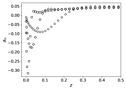
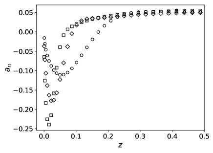
Figure 1: Coefficients $a_{n}$, plotted at locations $z_{n}$, for $\mathrm{Ta}=10^{4}$ (circles), $10^{6}$ (diamonds) and $10^{8}$ (squares) and a resolution $N=64$. The boundary conditions are no slip (left panel) and stress free (right panel). The Rayleigh number is in all cases approximately 4 times critical: $\mathrm{Ra}=34.92\mathrm{Ta}^{2/3}$.

The result is an SDP which yields the desired optimal bound, but it is not completely straightforward to compare the optimal coefficients $\lambda_{n}$ to the optimal $\varphi(z)$ or $\tau(z)$ one might obtain from an analytical calculation. The reson for this is that the optimization problem includes constraints containing the integral of two functions $f(z)$ and $g(z)$, one of which (for example $f$) is replaced in the course of the discretization by a sum of Dirac $\delta$-functions as $\sum_{n=1}^{N}f_{n}\delta(z-z_{n})$ where the collocation points $z_{n}$ are given by

$$z_{n}=\frac{1}{2}\left[1+\cos\left(\pi\frac{n-1}{N-1}\right)\right]~{}~{}~{},~{}~{}~{}n=1...N.$$ (15)

The integral $\int f(z)g(z)dz$ then becomes the sum $\sum_{n=1}^{N}f_{n}g(z_{n})$. There is no immediate relationship between $f(z)$ and the $f_{n}$ if the $f_{n}$ are chosen such that the sum $\sum_{n=1}^{N}f_{n}g(z_{n})$ approximates as closely as possible the integral $\int f(z)g(z)dz$. For instance, these $f_{n}$ depend on the resolution $N$ and the collocation points $z_{n}$. The SDP as implemented returns a set of coefficients $a_{n}$ which appear in a representation of the first derivative of $\varphi(z)$ as $\varphi^{\prime}(z)=\sum_{n=1}^{N}a_{n}\delta(z-z_{n})$. The magnitude of these $a_{n}$ is not directly connected to optimal background fields obtained from analytical calculations, but the general dependence on space must be comparable.

Analytical treatment of infinite Prandtl number convection with the background field method Doering and Constantin (2001); Constantin and Doering (1999); Constantin, Hallstrom, and Putkaradze (1999); Plasting and Ierley (2005) used functions $\tau(z)$ or $\varphi(z)$ whose first derivative is either constant or piecewise constant, with a certain value for this derivative in the central region of the layer and another value in two boundary layers adjacent to the top and bottom boundaries. More sophisticated background fields were also used in the non rotating problem Doering, Otto, and Reznikoff (2006); Otto and Seis (2011). The thickness of the boundary layers is imposed by the Rayleigh number. Fig. 1 shows for a few examples the $a_{n}$, each $a_{n}$ plotted at the location $z_{n}$. The $a_{n}$ are approximately constant for the $z_{n}$ near the center of the layer, but there is a rapid variation of the $a_{n}$ within apparent boundary layers. More than one extremum appears for no slip boundaries at large $\mathrm{Ta}$. The thickness of the boundary layer for no slip boundaries, defined from the location of the minimal $a_{n}$, is compatible with the scaling in $\mathrm{Ta}^{-1/4}$ known from Ekman layers, whereas the layers remain thicker for free slip boundary conditions. The demand on resolution is therefore higher for no slip boundaries.

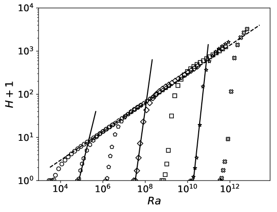
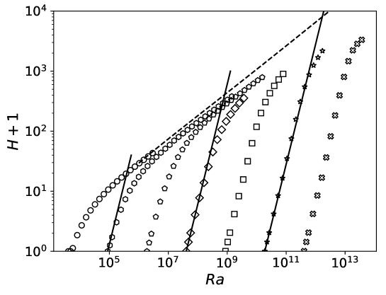
Figure 2: The bound on the Nusselt number $H+1$ as a function of $\mathrm{Ra}$ for $\mathrm{Ta}=10^{4}$ (circles), $10^{6}$ (hexagons), $10^{8}$ (pentagons), $10^{10}$ (diamonds), $10^{12}$ (squares), $10^{14}$ (stars) and $10^{16}$ (crosses). The upper panel is for no slip boundaries and the lower panel for stress free boundaries. The dashed lines are fits to bounds obtained for $\mathrm{Ta}=0$ (see Refs. Ierley, Kerswell, and Plasting, 2006; Tilgner, 2017) given by $H+1=0.101\times\mathrm{Ra}^{0.4}+0.70965\times\mathrm{Ra}^{0.2}-7.166$ for stress free boundaries and $H+1=0.139\times\mathrm{Ra}^{1/3}$ for no slip boundaries. The continuous lines show functions of the form $(\mathrm{Ra}/\mathrm{Ra}_{\mathrm{crit}})^{\beta}$ with $\mathrm{Ra}_{\mathrm{crit}}$ computed from the asymptotically valid expression Chandrasekhar (1961) $\mathrm{Ra}_{\mathrm{crit}}=8.73\times\mathrm{Ta}^{2/3}$ for stress free boundary conditions (upper panel) and obtained as part of the fitting procedure for no slip boundary conditions (lower panel). The exponent $\beta$ in the case of no slip boundaries is 3 ($\mathrm{Ta}=10^{6}$), 3.5 ($\mathrm{Ta}=10^{10}$) and 4.5 ($\mathrm{Ta}=10^{14}$), whereas $\beta=2$ for all lines drawn for stress free boundaries.

III Results

The bound $H$ on the advective heat transport is obtained from the selection $Z=\langle v_{z}\theta\rangle$. The results of experiments or numerical simulations are usually reported in terms of the Nusselt number, which is identical to $\langle\overline{v_{z}\theta}\rangle+1$. For easier comparison, fig. 2 shows $H+1$ as a function of $\mathrm{Ra}$ for various $\mathrm{Ta}$. The graphs have the general appearance familiar from experiments or numerical simulations: the bound $H$ is exactly zero for $\mathrm{Ra}$ less than the critical Rayleigh number $\mathrm{Ra}_{\mathrm{crit}}$ computed from linear stability analysis and the heat transport is reduced by rotation compared with the non rotating flows at Rayleigh numbers just above onset with a rapid increase of $H+1$ as a function of $\mathrm{Ra}$, whereas at sufficiently large $\mathrm{Ra}$, $H+1$ increases more slowly as a function of $\mathrm{Ra}$ at a rate asymptotically identical with the non rotating case. For no slip boundaries, there is an overshoot in the sense that the bound for rotating convection is actually larger than that for the non rotating case in an intermediate interval of $\mathrm{Ra}$. This echoes the behaviour known from experiments and simulations in which the Nusselt number of rotating convection may exceed the Nusselt number of non rotating convection Zhong, Ecke, and Steinberg (1993); Zhong et al. (2009); Schmitz and Tilgner (2010), a behaviour that is not observed for stress free boundaries Schmitz and Tilgner (2009).

There does not seem to be any numerical data available for strictly infinite $\mathrm{Pr}$, but the results in Ref. King et al., 2009 suggest that there is no significant difference in the Nusselt number in going from $\mathrm{Pr}=7$ to $\mathrm{Pr}=100$ so that it is meaningful to compare data obtained for $\mathrm{Pr}$ equal to 7 or larger to the bounds for infinite $\mathrm{Pr}$. The bounds for no slip boundaries in fig. 2 may then directly be compared to the data compiled in figure 1 of Ref. Julien et al., 2016. It is frequently attempted to fit power laws to experimentally or numerically determined values of the Nusselt number. Power laws are not a terribly good fit to either $H$ or the bounds $H+1$ in fig. 2 in the rotation dominated regime, but if one insists on fitting power laws to the dependence of $H+1$ on $\mathrm{Ra}$, one finds for no slip boundaries exponents of 2, 3.5 and 4.5 at approximately the Taylor numbers at which the exponents for the actual Nusselt number at $\mathrm{Pr}=7$ are 1.2, 3 and 3.6 according to Ref. Julien et al., 2016. The bounds parallel the behaviour of the Nusselt number in that larger exponents are necessary at larger $\mathrm{Ta}$, but the exponents obtained from fits to the bounds are systematically larger than those obtained from the experiments.

For free slip boundaries, the dependence of $H+1$ on $\mathrm{Ra}$ for $\mathrm{Ra}$ just above $\mathrm{Ra}_{\mathrm{crit}}$ is reasonably fitted by $H+1=(\mathrm{Ra}/\mathrm{Ra}_{\mathrm{crit}})^{2}$ at all $\mathrm{Ta}$. From simulations Schmitz and Tilgner (2010) at $10^{2}\lesssim\mathrm{Ta}\lesssim 10^{8}$ one finds for $\mathrm{Pr}=7$ that the Nusselt number just above onset behaves approximately as $(\mathrm{Ra}/\mathrm{Ra}_{\mathrm{crit}})^{6/5}$, so that the exponents fitting the bounds again appear to be larger than what they should be if the bounds were sharp.

It is also seen in figs. 1 and 2 that for stress free boundaries, the non rotating behaviour is attained only at very large Rayleigh numbers, if at all. For infinite $\mathrm{Pr}$, it is not obvious why the behaviour of rotating and non rotating convection should approach each other at any $\mathrm{Ra}$. We currently do not have a solid understanding of the mechanism which determines the transition from convection dominated by Coriolis force to convection nearly independent of rotation as $\mathrm{Ra}$ is increased. King et al. (2009) suggested that the transition occurs when the Ekman layer and thermal boundary layer are equally thick. However, this criterion cannot be generally applicable because the same transition is observed for stress free and for no slip boundary conditions Schmitz and Tilgner (2009, 2010) and there are no Ekman layers near the stress free boundaries. The most intuitive criterion is based on the Rossby number. If this number is large, the Coriolis term is small compared with the advection term in the momentum equation. Horn and Shishkina (2015) classified states of rotating convection with the help of the Rossby number based on the free fall velocity, $(g\alpha\Delta Th)^{1/2}/(\Omega h)\propto(\mathrm{Ra}/(\mathrm{Pr}\mathrm{Ta}))^{1/2}$. This number is always zero in the model of convection at infinite Prandtl number, which is not surprising because there is no advection term left in the momentum equation compared to which the Coriolis term could be small. It is also known Schmitz and Tilgner (2009, 2010) that if the Rossby number is based on the actual flow velocity rather than the free fall velocity, the Rossby number does not allow one to distinguish at $\mathrm{Pr}=0.7$ or $\mathrm{Pr}=7$ between convection dominated by rotation from convection nearly independent of rotation. The balance between Coriolis and rotation terms does not seem to be essential for the transition.

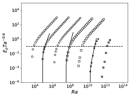
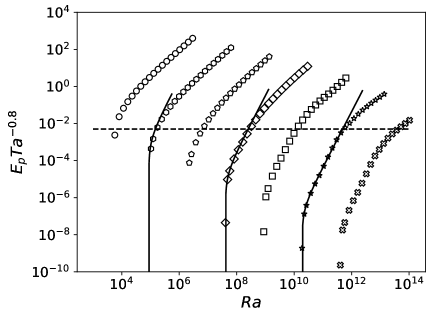
Figure 3: The bound $E_{p}$ on the poloidal energy shown in the combination $E_{p}\mathrm{Ta}^{-0.6}$ for no slip boundaries (left panel) and $E_{p}\mathrm{Ta}^{-0.8}$ for stress free boundaries (right panel) with the same symbols as in fig. 2. The continuous lines indicate the functions $(\mathrm{Ra}/\mathrm{Ra}_{\mathrm{crit}})[(\mathrm{Ra}/\mathrm{Ra}_{\mathrm{crit}})^{\beta}-1]\mathrm{Ta}^{1/3}$ for $\beta=2$, $3.5$ and $4.5$ in the left panel and $\beta=2$ in the right panel. The dashed horizontal lines are located at $E_{p}\mathrm{Ta}^{-0.6}=0.1$ (left panel) and $E_{p}\mathrm{Ta}^{-0.8}=5\times 10^{-3}$ (right panel).

Another reasoning, put forward by Schmitz and Tilgner (2009), combines the asymptotic behaviour of the Nusselt number at small and large $\mathrm{Ra}$ for fixed $\mathrm{Ta}$ to predict that the transition should occur if

$$(E_{\mathrm{pol}}+E_{\mathrm{tor}})\mathrm{Ta}^{-1}=\mathrm{const.}$$ (16)

This criterion, which is valid for both types of boundary conditions Schmitz and Tilgner (2010), is independent of $\mathrm{Pr}$ and can be immediately extended to infinite $\mathrm{Pr}$. This criterion also motivates the form in which the bounds are presented in the following two figures.

Figs. 3 and 4 show the bounds on poloidal and toroidal energies, $E_{p}$ and $E_{t}$, obtained from $Z=\langle\frac{1}{2}|\nabla\times\nabla\times(\phi\bm{\hat{z}})|^{2}\rangle$ and $Z=\langle\frac{1}{2}|\nabla\times(\psi\bm{\hat{z}})|^{2}\rangle$, respectively. At any $\mathrm{Ta}$, these bounds show again two regions of $\mathrm{Ra}$ in which rotation is either suppressing convection or not. To better identify the interval of $\mathrm{Ra}$ dominated by rotation, it helps to make a connection with the bounds on the heat transport. The $z$ component of velocity is zero at the boundaries so that the bound $H$ implies by virtue of the Poincaré inequality a bound on the poloidal energy Tilgner (2017) as

$$E_{\mathrm{pol}}\leq\frac{1}{2\pi^{2}}\mathrm{Ra}H.$$ (17)

However, one expects a stricter bound to be valid. Taking the dot product of the momentum equation (2) with $\bm{v}$ and integrating over space leads to

$$\sum_{ij}\langle(\partial_{j}v_{i})^{2}\rangle=\mathrm{Ra}\langle v_{z}\theta\rangle.$$ (18)

If $\lambda_{c}$ is a characteristic length scale of the flow, one expects $\sum_{ij}\langle(\partial_{j}v_{i})^{2}\rangle\sim(E_{\mathrm{pol}}+E_{\mathrm{tor}})/\lambda_{c}^{2}$ and therefore $E_{\mathrm{pol}}\leq\mathrm{Ra}H/\lambda_{c}^{2}$. At $\mathrm{Ra}$ just above critical, the typical length scale of rotation is the wavelength of the most unstable mode in linear stability analysis, which leads toChandrasekhar (1961) $\lambda_{c}^{2}\propto\mathrm{Ta}^{-1/3}$. Replacing $H$ by its power law fit deduced from fig. 2 and using $\mathrm{Ra}/\mathrm{Ra}_{\mathrm{crit}}$ as variable, one expects the existence of a bound $E_{p}$ of the form

$$E_{\mathrm{pol}}\leq E_{p}\propto\frac{\mathrm{Ra}}{\mathrm{Ra}_{\mathrm{crit}}}\left[\left(\frac{\mathrm{Ra}}{\mathrm{Ra}_{\mathrm{crit}}}\right)^{\beta}-1\right]\mathrm{Ta}^{1/3}$$ (19)

This functional form, with a prefactor equal to 1, fits well the dependence of $E_{p}$ on $\mathrm{Ra}$ for rotating convection with both types of boundary conditions and $\mathrm{Ra}$ close to $\mathrm{Ra}_{\mathrm{crit}}$. The bound $E_{p}$ obtained from the SDP is therefore sensitive to the variation of the characteristic length scale of convection with $\mathrm{Ta}$, in agreement with analytically computed bounds Tilgner (2022).

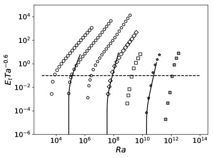
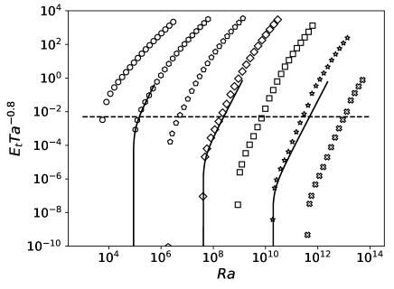
Figure 4: The bound on the toroidal energy, $E_{t}$, in the same representation as $E_{p}$ in fig. 3, with the same symbols and the same dashed and continuous lines. The left panel is for no slip boundaries and the right panel for stress free boundaries.

Eq. (19) fails to be a good fit if $\mathrm{Ra}$ is large enough, which marks the upper edge of the interval of $\mathrm{Ra}$ in which the bound $E_{p}$ is controlled by the Coriolis force. Fig. 3 shows that the bound on $E_{\mathrm{pol}}$ is indicative of rapidly rotating convection only if $E_{p}\mathrm{Ta}^{-0.6}\leq 0.1$ for no slip and $E_{p}\mathrm{Ta}^{-0.8}\leq 5\times 10^{-3}$ for stress free boundaries. Fig. 4 repeats all the previous considerations for the toroidal energy. For no slip boundaries, the same function as in eq. (19) approximates also the bounds for the toroidal energy in the rapidly rotating regime, which implies near equipartition between the poloidal and toroidal energies in as far as bounds are concerned. In the case of stress free boundaries, the bound on toroidal energy $E_{t}$ exceeds the bound on poloidal energy. For both boundary conditions, $E_{t}$ exceeds $E_{p}$ in the high Rayleigh number regime even though the toroidal energy is zero in the non rotating case. At finite $\mathrm{Pr}$, simulations Horn and Shishkina (2015) show that the fraction of toroidal to total energy decreases with $\mathrm{Ra}$ at large $\mathrm{Ra}$. This behavior is not reproduced by the bound $E_{t}$, possibly because eq. (6) prevents the fraction of toroidal to total energy from decreasing to zero which would mean that in this particular respect, rotating convection at infinite and finite $\mathrm{Pr}$ are fundamentally different from each other. Fig. 4 also shows that for no slip boundaries, the condition $E_{t}\mathrm{Ta}^{-0.6}\leq\mathrm{const.}$ reasonably delimits the region in parameter space in which the bound $E_{t}$ is determined by the length scale of rapidly rotating convection near onset, $\lambda_{c}$. Combined with the bounds for poloidal energy, this leads to $(E_{p}+E_{t})\mathrm{Ta}^{-0.6}\leq\mathrm{const.}$ as a criterion for the bounds being mainly controlled by the Coriolis term, which contains a different exponent than eq. (16).

IV Summary

Predictions of heat transport in turbulent convection necessarily rely on empirically motivated assumptions. An early approach assumed that the thermal boundary layers are marginally stable which leads in the non rotating case to Malkus and Chandrasekhar (1954); Howard (1966) $\mathrm{Nu}\propto\mathrm{Ra}^{1/3}$. It is possible to derive bounds that come at least to within logarithmic factors of $\mathrm{Ra}^{1/3}$ for convection at infinite Prandtl number Chan (1971); Ierley, Kerswell, and Plasting (2006); Constantin and Doering (1999); Doering, Otto, and Reznikoff (2006); Otto and Seis (2011). Bounds for convection at arbitrary Prandtl number Doering and Constantin (1996) are no better than $\mathrm{Nu}\propto\mathrm{Ra}^{1/2}$. It is tempting to ascribe this difference to the different nature of the equations of evolution: the momentum equation becomes a diagnostic equation at infinite $\mathrm{Pr}$, effectively reducing the problem to a single equation for the temperature field. It is then interesting to investigate whether similarly tight bounds can be derived for rotating convection at infinite $\mathrm{Pr}$.

Attempts at analytically deriving bounds on heat transport in rotating convection at infinite $\mathrm{Pr}$ have been based on the background field method Doering and Constantin (2001); Constantin, Hallstrom, and Putkaradze (1999) which enforces constraints derived from the surface average over horizontal planes of the temperature equation and the volume average of the temperature equation multiplied by $\theta$. The numerical search of an optimal bound satisfying constraints of this form leads to an SDP. For $\mathrm{Ta}=0$ and no slip boundaries, the SDP technique finds an upper bound for the heat transport which varies as a function of $\mathrm{Ra}$ as $\mathrm{Ra}^{1/3}$, at least to within logarithmic factors Nobili and Otto (2017). Heat transport is reduced by rotation. This reduction is reproduced in the bound computation, but not by as much as is observed in numerical computations at finite but large $\mathrm{Pr}$. The SDP finds the correct $\mathrm{Ra}$ for the onset of convection, but at larger $\mathrm{Ra}$, the bound on $\mathrm{Nu}$ increases more rapidly with $\mathrm{Ra}$ than the $\mathrm{Nu}$ obtained from simulations. The mere fact that momentum equation is reduced to a diagnostic equation is therefore no guarantee that the background method will provide us with satisfactory bounds.

The bounds obtained from the SDP are nonetheless stricter than the bounds obtained from analytical work in as far as the dependence on rotation is concerned. Both types of calculations enforce the same constraints, but the SDP optimizes the background field profile and does not rely on simplifying estimates to ensure the validity of inequalities analogous to (13) usually called spectral constraint in the context of the background method. Linear stability theory computes a critical Rayleigh number $\mathrm{Ra}_{\mathrm{crit}}$ which asymptotically scales with $\mathrm{Ta}$ as $\mathrm{Ra}_{\mathrm{crit}}\propto\mathrm{Ta}^{2/3}$ at large $\mathrm{Ta}$. For stress free boundaries, the result from the SDP may be presented as $\mathrm{Nu}\lesssim\left(\mathrm{Ra}/\mathrm{Ra}_{\mathrm{crit}}\right)^{2}$ ignoring numerical prefactors. The rotation dependent bounds obtained analytically are either $\mathrm{Nu}-1\lesssim\mathrm{Ra}^{1/2}\left(\mathrm{Ra}/\mathrm{Ra}_{\mathrm{crit}}\right)^{1/2}$ from Ref. Tilgner, 2022 or $\mathrm{Nu}-1\lesssim\mathrm{Ra}^{1/2}\left(\mathrm{Ra}/\mathrm{Ra}_{\mathrm{crit}}\right)^{3/2}$ from Ref. Constantin, Hallstrom, and Putkaradze, 1999 in the rotation dominated regime. Both of these bounds impose a weaker reduction of $\mathrm{Nu}$ with $\mathrm{Ta}$ than the bound from the SDP. The expressions for no slip boundaries are more complicated since the analytical result Constantin, Hallstrom, and Putkaradze (1999) for the bound on $\mathrm{Nu}-1$ is a sum of two terms, one varying as $\mathrm{Ra}^{1/2}\left(\mathrm{Ra}/\mathrm{Ra}_{\mathrm{crit}}\right)^{3/2}$, the other as $\mathrm{Ra}^{5/4}\left(\mathrm{Ra}/\mathrm{Ra}_{\mathrm{crit}}\right)^{3/4}$. Both terms decrease more slowly with increasing $\mathrm{Ta}$ as the $\left(\mathrm{Ra}/\mathrm{Ra}_{\mathrm{crit}}\right)^{\beta}$ with $\beta>2$ in fig. 2.

The SDP bounds the advective heat flux to zero for $\mathrm{Ra}<\mathrm{Ra}_{\mathrm{crit}}$. The SDP bounds also reflect several qualitative effects known from experiments and numerical simulations, such as a characteristic length scale varying as $\mathrm{Ta}^{-1/6}$ in the rotation dominated regime. In the case of no slip boundaries, the heat transport in rapidly rotating convection and in some interval of Rayleigh numbers exceeds the heat transport of non rotating convection at the same Rayleigh numbers. The exponent $\beta$ in $\mathrm{Nu}\lesssim\left(\mathrm{Ra}/\mathrm{Ra}_{\mathrm{crit}}\right)^{\beta}$ in the bounds for no slip boundary conditions increases with $\mathrm{Ta}$ (see fig. 2), just as it does in fits to experimentally and numerically determined $\mathrm{Nu}$.

Rotating convection at infinite Prandtl number thus is a system in which significant improvement over existing analytical results is possible within the background method. It is also a system which is a promising testing ground for bounding methods involving additional constraints. It is possible to formulate an SDP which takes into account more constraints Chernyshenko et al. (2014), but at the cost of a significantly larger computational burden. A method of this type was recently demonstrated in the context of nonlinear stability analysis Fuentes, Goluskin, and Chernyshenko (2022). Rotating convection at infinite Prandtl number is a non trivial fluid dynamic system, which is relatively simple in the sense that it is governed by an equation for a single scalar field, and for which the known bounds do not scale with the control parameters in the same way as the results of numerical computations, so that this system promises to be particularly rewarding for any improved bounding method.

References

- Hopf (1941) E. Hopf, “Ein allgemeiner Endlichkeitssatz der Hydrodynamik,” Mathematische Annalen 117, 764–775 (1941).
- Doering and Constantin (1992) C. Doering and P. Constantin, “Energy dissipation in shear driven turbulence,” Phys. Rev. Lett. 69, 1648–1651 (1992).
- Doering and Constantin (1996) C. Doering and P. Constantin, “Variational bounds on energy dissipation in incompressible flows:III. Convection,” Phys. Rev. E 53, 5957–5981 (1996).
- Fantuzzi, Arslan, and Wynn (2022) G. Fantuzzi, A. Arslan, and A. Wynn, “The background method: theory and computations,” Philosophical Transactions of the Royal Society A: Mathematical, Physical and Engineering Sciences 380, 20210038 (2022).
- Malkus (1956) W. Malkus, “Outline for a theory for turbulent shear flow,” J. Fluid Mech. 1, 521–539 (1956).
- Howard (1963) L. Howard, “Heat transport by turbulent convection,” J. Fluid Mech. 17, 405–432 (1963).
- Busse (1969) F. Busse, “On Howard’s upper bound for heat transport by turbulent convection,” J. Fluid Mech. 37, 457–477 (1969).
- Kerswell (2001) R. Kerswell, “New results in the variational approach to turbulent Boussinesq convection,” Phys. Fluids 13, 192–209 (2001).
- Grooms and Whitehead (2014) I. Grooms and J. P. Whitehead, “Bounds on heat transport in rapidly rotating Rayleigh–Bénard convection,” Nonlinearity 28, 29–41 (2014).
- Pachev et al. (2020) B. Pachev, J. P. Whitehead, G. Fantuzzi, and I. Grooms, “Rigorous bounds on the heat transport of rotating convection with Ekman pumping,” Journal of Mathematical Physics 61, 023101 (2020).
- Jones (2015) C. Jones, “Thermal and compositional convection in the outer core,” in Treatise on Geophysics, 2nd edition, Vol. 8, edited by G. Schubert (Elsevier, 2015) pp. 115–159.
- Tilgner (2022) A. Tilgner, “Bounds for rotating Rayleigh-Bénard convection at large Prandtl number,” Journal of Fluid Mechanics 930, A33 (2022).
- Doering and Constantin (2001) C. Doering and P. Constantin, “On upper bounds for infinite Prandtl number convection with or without rotation,” J. Math. Phys. 42, 784–795 (2001).
- Constantin, Hallstrom, and Putkaradze (1999) P. Constantin, C. Hallstrom, and V. Putkaradze, “Heat transport in rotating convection,” Physica D 125, 275–284 (1999).
- Vitanov (2003) N. Vitanov, “Convective heat transport in a rotating fluid layer of infinite Prandtl number: Optimum fields and upper bound on Nusselt number,” Phys. Rev. E 67, 026322 (2003).
- Plasting and Ierley (2005) C. Plasting and G. Ierley, “Infinite-Prandtl-number convection. Part 1. Conservative bounds,” J. Fluid Mech. 542, 343–363 (2005).
- Ierley, Kerswell, and Plasting (2006) G. Ierley, R. Kerswell, and C. Plasting, “Infinite-Prandtl-number convection. Part 2. A singular limit of upper bound theory,” J. Fluid Mech. 560, 159–227 (2006).
- Tilgner (2017) A. Tilgner, “Bounds on poloidal kinetic energy in plane layer convection,” Phys. Rev. Fluids 2, 123502 (2017).
- Tilgner (2019) A. Tilgner, “Time evolution equation for advective heat transport as a constraint for optimal bounds in Rayleigh-Bénard convection,” Phys. Rev. Fluids 4, 014601 (2019).
- Chernyshenko et al. (2014) S. Chernyshenko, P. Goulart, D. Huang, and Papachristodoulou, “Polynomial sum of squares in fluid dynamics: a review with a look ahead,” Phil. Trans. Roy. Soc. A 372, 20130350 (2014).
- Constantin and Doering (1999) P. Constantin and C. Doering, “Infinite Prandtl number convection,” J. Stat. Phys. 94, 159–172 (1999).
- Doering, Otto, and Reznikoff (2006) C. Doering, F. Otto, and M. Reznikoff, “Bounds on vertical heat transport for infinite-Prandtl-number Rayleigh-Bénard convection,” J. Fluid Mech. 560, 229–241 (2006).
- Otto and Seis (2011) F. Otto and C. Seis, “Rayleigh-Bénard convection: Improved bounds on the Nusselt number,” J. Math. Phys. 52, 083702 (2011).
- Chandrasekhar (1961) S. Chandrasekhar, Hydrodynamic and Hydromagnetic Stability (Oxford University Press, Oxford, 1961).
- Zhong, Ecke, and Steinberg (1993) F. Zhong, R. E. Ecke, and V. Steinberg, “Rotating Rayleigh-Bénard convection: asymmetric modes and vortex states,” J. Fluid Mech. 249, 135–159 (1993).
- Zhong et al. (2009) J.-Q. Zhong, R. J. A. M. Stevens, H. J. H. Clercx, R. Verzicco, D. Lohse, and G. Ahlers, “Prandtl-, Rayleigh-, and Rossby-Number Dependence of Heat Transport in Turbulent Rotating Rayleigh-Bénard Convection,” Phys. Rev. Lett. 102, 044502 (2009).
- Schmitz and Tilgner (2010) S. Schmitz and A. Tilgner, “Transitions in turbulent rotating Rayleigh-Bénard convection,” Geophys. Astrophys. Fluid Dyn. 104, 481–489 (2010).
- Schmitz and Tilgner (2009) S. Schmitz and A. Tilgner, “Heat transport in rotating convection without Ekman layers,” Phys. Rev. E 80, 015305(R) (2009).
- King et al. (2009) E. M. King, S. Stellmach, J. Noir, U. Hansen, and J. M. Aurnou, “Boundary layer control of rotating convection systems,” Nature 457, 301–304 (2009).
- Julien et al. (2016) K. Julien, J. M. Aurnou, M. A. Calkins, E. Knobloch, P. Marti, S. Stellmach, and G. M. Vasil, “A nonlinear model for rotationally constrained convection with Ekman pumping,” Journal of Fluid Mechanics 798, 50–87 (2016).
- Horn and Shishkina (2015) S. Horn and O. Shishkina, “Toroidal and poloidal energy in rotating Rayleigh-Bénard convection,” Journal of Fluid Mechanics 762, 232–255 (2015).
- Malkus and Chandrasekhar (1954) W. V. R. Malkus and S. Chandrasekhar, “The heat transport and spectrum of thermal turbulence,” Proceedings of the Royal Society of London. Series A. Mathematical and Physical Sciences 225, 196–212 (1954).
- Howard (1966) L. N. Howard, “Convection at high Rayleigh number,” in Applied Mechanics, edited by H. Görtler (Springer Berlin Heidelberg, Berlin, Heidelberg, 1966) pp. 1109–1115.
- Chan (1971) S. Chan, “Infinite Prandtl number turbulent convection,” Stud. Appl. Maths 50, 13–49 (1971).
- Nobili and Otto (2017) C. Nobili and F. Otto, “Limitations of the background field method applied to Rayleigh-Bénard convection,” J. Math. Phys. 58, 093102 (2017).
- Fuentes, Goluskin, and Chernyshenko (2022) F. Fuentes, D. Goluskin, and S. Chernyshenko, “Global stability of fluid flows despite transient growth of energy,” Phys. Rev. Lett. 128, 204502 (2022).