The variance of a general class of multiplicative functions in short intervals

Abstract.

We study a general class of multiplicative functions by relating “short averages” to its “long average”. More precisely, we estimate asymptotically the variance of such a class of functions in short intervals using Fourier analysis and counting rational points on certain binary forms. Our result is applicable to the interesting multiplicative functions $\mu_{k}(n),\frac{\varphi(n)}{n},\frac{n}{\varphi(n)},$ $\mu^{2}(n)\frac{\varphi(n)}{n}$, $\sigma_{\alpha}(n)$, $(-1)^{\#\{p\,:\,p^{k}|n\}}$ and many others that establish various new results and improvements in short intervals to the literature.

1. Introduction

Some of the most exciting arithmetical functions to the number theorists are multiplicative functions, which satisfy $f(mn)=f(m)f(n)$ for all $(m,n)=1$. One of the main themes in analytic number theory is to evaluate asymptotically the global partial sum $\sum_{n\leq x}f(n)$ for any multiplicative function $f$. The global behavior of multiplicative functions is well studied although it is very difficult to obtain a good understanding of such partial sums. One may ask whether similar results hold for the “local” behavior of multiplicative functions. In particular, one may try to obtain an asymptotic formula for the following short interval sum

$$\sum_{x\leq n\leq x+H}f(n)$$

under suitable growth conditions on the interval of length $H$.

Work of Matomäki, Radziwiłł and Tao

In a breakthrough work, Matomäki and Radziwiłł  [21] showed that for any multiplicative function $f:\mathbb{N}\to[-1,1]$, the short average is close to its long average for almost all $x\leq X$ in the sense that

$$\bigg{|}\sum_{x<n\leq x+H}f(n)-\frac{H}{X}\sum_{n\leq X}f(n)\bigg{|}=o(H),\quad\text{ as }\,H=H(X)\to\infty.$$

This result has many applications, such as the average of the Liouville function, the counting of smooth numbers in short intervals, and the number of sign changes of the Liouville function up to $X$. Further, Matomäki, Radziwiłł, and Tao [Theorem A.1, [22]] extend this result for any non-pretentious multiplicative function $f:\mathbb{N}\to\mathbb{C}$ bounded by $1$.

Work of Gorodetsky, Matomäki, Radziwiłł and Rodgers

Recently, Gorodetsky et al. [7] studied the behaviour of square-free numbers in shorts intervals, in particular, they showed that for a given $\epsilon\in(0,1/100)$ and $2\leq H\leq X^{6/11-\epsilon}$,

$$\sum_{x<n\leq x+H}\mu^{2}(n)=\frac{H}{\zeta(2)}+O\left(H^{\frac{1}{4}}\right)$$

holds for almost all $x\leq X$.

Observe that, the number of square-free integers in almost all intervals have $H^{3/4}$ cancellation to its mean compare to work of Matomäki, Radziwiłł and Tao, which has $o(1)$ cancellation to its mean for Liouville or Möbius function; although they have a better range for short intervals. This kind of phenomenon is happening due to the rigidity of the sequences of square-free integers, whereas the sequence of Liouville or Möbius function is not rigid.

General class of multiplicative functions

The objective of the present paper is to introduce general classes of multiplicative functions and study their local behaviour. This leads us to obtain local behaviour of many interesting multiplicative functions which are discussed in Subsection 1.3.

We denote $\mathcal{M}$ as the set of all multiplicative functions and $\mathcal{G}$ as the set of all completely multiplicative functions. For a parameter $\alpha\geq 0$, we define

$$\mathcal{M}_{\alpha}^{\mu}=\Big{\{}h\in\mathcal{M}:\,h(d)=\mu(d)\frac{g(d)}{d^{\alpha}},\,g\in\mathcal{M}\Big{\}}\quad\text{ and }\quad\mathcal{G}_{\alpha}=\Big{\{}h\in\mathcal{G}:\,h(d)=\frac{g(d)}{d^{\alpha}}\Big{\}}.$$

Let $\mathcal{P}^{\text{fin}}$ be any finite set of primes and $\beta,\eta\in\mathbb{C}$. A function $h\in\mathcal{M}_{\alpha}^{\mu}\cup\mathcal{G}_{\alpha}$ is said to satisfy the property $(A)$ if

$$g(p)= \left\{\begin{array}[c]{ll}\pm\beta&\,\text{ if }p\not\in\mathcal{P}^{\text{fin}},\\ \eta&\,\text{ if }p\in\mathcal{P}^{\text{fin}}.\end{array}\right.$$

Here and throughout we assume that for an integer $k\geq 1$ and a real number $0\leq\alpha<2$, the condition $\alpha+k>\frac{3}{2}$ holds. Now we consider the following class of functions:

$$\mathcal{F}_{\alpha,\beta,k}=\bigg{\{}f\in\mathcal{M}:f(n)=\sum_{d^{k}|n}h(d),\,h\in\mathcal{M}_{\alpha}^{\mu}\cup\mathcal{G}_{\alpha}\text{ and }\text{satisfies }(A)\bigg{\}}.$$

Remark 1.

In the above class, we see that $g(d)\ll d^{\epsilon}$ for any $\epsilon>0$ arbitrary small. The class $\mathcal{F}_{\alpha,\beta,k}$ is a generalization to the functions of type $f=1*h$ and examples of this class are given in the next subsection. Also one can extend the nature of $g(p)$ by supplying different values on a given finite set of primes.

1.1. Mean values for class $\mathcal{F}_{\alpha,\beta,k}$

Given a multiplicative function $f$ it is desired to obtain an asymptotic formula for the sum $\sum_{n\leq x}f(n)$. Ideally, one would like to give such formula with explicit error term to the above mean value which depends only on a knowledge of $f(p)$ for primes $p$.

Let $x\geq 1$ and $f\in\mathcal{F}_{\alpha,\beta,k}$. It is easy to see that for any $\epsilon>0$,

(1.1) $$\sum_{n\leq x}f(n)=\widetilde{c}_{h,k}x+O\left(x^{\max\big{\{}\frac{1-\alpha}{k}+\epsilon,\,0\big{\}}}\right),$$

where

(1.2) $$\widetilde{c}_{h,k}=\sum_{d\geq 1}\frac{h(d)}{d^{k}}.$$

The improvements on the error term for various arithmetical functions belonging to $\mathcal{F}_{\alpha,\beta,k}$ are obtained in [1], [13], [14], [19], [24], [30] and [35] etc.

Remark 2.

We are restricting ourselves to $\alpha<2$ since when $\alpha\geq 2$ then the behaviour of corresponding arithmetic functions become straightforward and thus omit it.

1.1.1. Examples

The class $\mathcal{F}_{\alpha,\beta,k}$ contains the following important arithmetical functions in the literature; namely, the indicator function of $k$-free integers $\mu_{k}(n)$, $\frac{\varphi(n)}{n}$, $\frac{n}{\varphi(n)}$, $\sigma_{s}(n)$, $\frac{J_{s}(n)}{n^{s}}$ where $\varphi$ is the usual Euler phi function, $\sigma_{s}(n)$ is the generalized divisor function and $J_{s}(n)$ is the Jordan totient function with $s\in\mathbb{C}$, and more examples are given in Section 1.3.

1.2. Mean values for class $\mathcal{F}_{\alpha,\beta,k}$ in short intervals

By “short intervals” means the sum $\sum_{x<n\leq x+H}f(n)$ where $2\leq H\leq x$ are large real numbers with $H=o(x)$ as $x\to\infty$. For the class $f\in\mathcal{F}_{0,\beta,2}$, Varbanec [34] obtained that for any $\epsilon>0$,

$$\sum_{x<n\leq x+H}f(n)=\widetilde{c}_{h,2}H+O(H^{1/2}x^{\epsilon})+O(x^{\theta+\epsilon}),$$

uniformly in $H<x$ and $\theta=0.2204.$

We can see that the error term is of order $O(H^{1/2+\epsilon})$ uniformly for $H\leq x$. In this article, we obtain an error term of size $O(H^{\frac{1-2\alpha}{2k}+\epsilon})$ with $\alpha\in[0,1/2)$ and $O(1)$ with $\alpha\in(1/2,2)$ for the family $\mathcal{F}_{\alpha,\beta,k}$, in different ranges of $H$ unconditionally and under the Lindelöf hypothesis for almost all $x\in[X,2X]$.

Exponents of short intervals

In order to state our results precisely we illustrate the exponents of short intervals depend on $\alpha$ and $k$. For $k\geq 3$, we define a function $\nu:=\nu(k,\alpha)$ by

(1.3) $$\nu=\begin{cases}\frac{-(2k-5/2+5\alpha)+\sqrt{(2k-5/2+5\alpha)^{2}+4k(k-2)(k+2\alpha-1)(2k-5/2+5\alpha)}}{2(k-2)(k+2\alpha-1)}&\mbox{ if }\alpha\in[0,1/2),\\ \frac{-2\alpha+2\sqrt{\alpha^{2}+\alpha k(k-2)}}{k-2}&\mbox{ if }\,\alpha\in(1/2,1).\end{cases}$$

Let $\alpha\in[0,1/2)$. On the basis of $\nu$, we characterize exponents $e$ and $g$ as follows:

(1.4) $$e(k,\alpha)=\begin{cases}\frac{2(3+8\alpha)}{11(1+2\alpha)}&\mbox{ if }k=2,\vspace{2mm}\\ \frac{2(k-\nu)(k+2\alpha-5/4)}{((4-\nu)k-2\nu)(k+2\alpha-1)}&\mbox{ if }k\geq 3,\end{cases}\quad\mbox{and}\quad g(k)=\begin{cases}\frac{2}{3}&\mbox{ if }\,k=2,\\ \frac{\sqrt{2k^{2}-4k+1}-1}{2\sqrt{2k^{2}-4k+1}-k}&\mbox{ if }\,k\geq 3.\end{cases}$$

For $\alpha\in(1/2,1)$, the exponents are defined by

(1.5) $$\widehat{e}(k,\alpha)=\begin{cases}\frac{29}{113-84\alpha}&\mbox{ if }\,k=1,\\ \min\big{\{}\frac{2+\alpha}{4},\frac{29}{71-42\alpha}\big{\}}&\mbox{ if }\,k=2,\\ \frac{\nu(k+\alpha-5/4)}{2k(\nu-\alpha)}&\mbox{ if }\,k\geq 3,\end{cases}\quad\mbox{ and }\quad\widehat{g}(k,\alpha)=\begin{cases}\frac{1}{3-2\alpha}&\mbox{ if }\,k=1,\\ \frac{2+\alpha}{4}&\mbox{ if }\,k=2,\\ \frac{\nu}{2(\nu-\alpha)}&\mbox{ if }\,k\geq 3.\end{cases}$$

Also for $\alpha\in[1,2)$,

(1.6) $$\widehat{e}(k,\alpha)=\widehat{g}(k,\alpha)=\begin{cases}1&\mbox{ if }\,k\neq 2,\\ \frac{2+\alpha}{4}&\mbox{ if }\,k=2.\end{cases}$$

We plot these exponents in Figure 2 and Figure 2 for a few fixed values of $\alpha$ and $k$ varies from 1 to 100.

1.2.1. Main results

We are now in a position to state our main results by using parameters from section 2.

Theorem 1.1.

Let $\epsilon>0$ be small and $f\in\mathcal{F}_{\alpha,\beta,k}$ with $0\leq\alpha<1/2$. Suppose that $2\leq H\leq X^{e(k,\alpha)-\epsilon}$. For almost all $x\in[X,2X]$ we have

$$\sum_{x<n\leq x+H}f(n)=\widetilde{c}_{h,k}H+O\Big{(}H^{\frac{1-2\alpha}{2k}}\big{(}\log H\big{)}^{\frac{\Re(\beta^{2})-1}{2}}\Big{)},$$

where $\widetilde{c}_{h,k}$ is defined by (1.2). Under the Lindelöf hypothesis, the above estimate holds in the wider range $H\leq X^{g(k)-\epsilon}$.

Theorem 1.2.

Assume that $f\in\mathcal{F}_{\alpha,\beta,k}$ with $1/2<\alpha<2$ and $\beta\in\mathbb{Z}\setminus\{0\}$. Let $\epsilon>0$ be small and $2\leq H\leq X^{\widehat{e}(k,\alpha)-\epsilon}$. For almost all $x\in[X,2X]$ we have

$$\sum_{x<n\leq x+H}f(n)=\widetilde{c}_{h,k}H+O(1).$$

Assuming the Lindelöf hypothesis, the above estimate holds in the wider range $H\leq X^{\widehat{g}(k,\alpha)-\epsilon}$.

To study the mean value of $f\in\mathcal{F}_{\alpha,\beta,k}$ in $(x,x+H]$, we compute the variance of its partial sum, from which the above theorems follow as an application of Chebyshev’s inequality.

Variance for the class $\mathcal{F}_{\alpha,\beta,k}$. We derive an asymptotic formula for variance of the form

(1.7) $$\operatorname{Var}{(\mathcal{F}_{\alpha,\beta,k})}:=\frac{1}{X}\int_{X}^{2X}\bigg{|}\sum_{x<n\leq x+H}f(n)-\widetilde{c}_{h,k}H\bigg{|}^{2}dx$$

for sufficiently large $X\geq 1$ and $\widetilde{c}_{h,k}$ is defined by (1.2).

Theorem 1.3.

Let $0\leq\alpha<1/2$ and $\beta\in\mathbb{Z}\setminus\{0\}$. Recall $e(k,\alpha)$ and $g(k)$ from (1.4). Let $0<\epsilon<\frac{3(1-2\alpha)}{2(\lceil\beta^{2}/12\rceil+4)}$ be given and $2\leq H\leq X^{e(k,\alpha)-\epsilon}$. Then

$$\operatorname{Var}(\mathcal{F}_{\alpha,\beta,k})=c_{h,k}H^{\frac{1-2\alpha}{k}}P_{\beta^{2}-1}(\log H)+O\left(H^{\frac{1-2\alpha}{k}-\delta_{k,\epsilon}}\right),$$

where $\delta_{2,\epsilon}=\frac{\epsilon}{8}$ and $\delta_{k,\epsilon}=\frac{\epsilon}{3(k+1)}$ for $k\geq 3$. Here $c_{h,k}$ and $P_{\beta^{2}-1}(\log H)$ are defined by (2.5) and (2.8) respectively.

Under the Lindelöf hypothesis, the above estimate holds in the wider range $H\leq X^{g(k)-\epsilon}$.

Note that Theorem 1.3 is valid for any given non-zero integer $\beta$. We shall extend the theorem to any complex $\beta$ with a weaker error term as follows.

Theorem 1.4.

Let $0\leq\alpha<1/2$ and $X\geq 1$ be sufficiently large. Suppose that $\beta\in\mathbb{C}\setminus\mathbb{Z}$ and $e(k,\alpha)$, $g(k)$ are defined by (1.4). For $2\leq H\leq X^{e(k,\alpha)-\epsilon}$ and $N\geq\lceil\Re(\beta^{2})\rceil$, we have

$$\operatorname{Var}(\mathcal{F}_{\alpha,\beta,k})=2H^{\frac{1-2\alpha}{k}}(\log H)^{\beta^{2}-1}\bigg{\{}\sum_{0\leq j\leq N}\frac{k^{j-\beta^{2}}\lambda_{j}(\beta^{2})}{\log^{j}H}+O\left(\frac{1}{\log^{N+1}H}\right)\bigg{\}},$$

where $\lambda_{j}(\beta^{2})$ is defined by (2.10). Under the Lindelöf hypothesis the above estimate holds in the wider range $H\leq X^{g(k)-\epsilon}$.

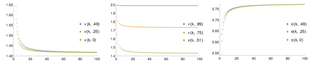
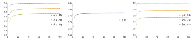
Figure 1. Plot $\nu(k,\alpha)$ and $e(k,\alpha)$ for a few fixed $\alpha$ and $k$ vary

Figure 2. Plot $\widehat{e}(k,\alpha)$, $g(k)$ and $\widehat{g}(k,\alpha)$ for a few fixed $\alpha$ and $k$ vary

Remark 3.

Following the proof of Theorem 1.3, we can extend our result to a subfamily $\{f(n)\}_{(n,q)=1}$ for any fixed integer $q\geq 1$ by looking at the mean square of

$$\sum_{\begin{subarray}{c}x<n\leq x+H\\ (n,q)=1\end{subarray}}f(n)-\frac{\varphi(q)}{q}\bigg{(}\sum_{(d,q)=1}\frac{h(d)}{d^{k}}\bigg{)}H.$$

In this case, we have the following changes into the constant $c_{h,k}$ (see (2.5)):

$$B(s)=\prod_{p\mid q}\left(1+\frac{2h(p)}{p^{k}}+\frac{h(p)^{2}}{p^{k+ks}}\right)^{-1}\prod_{p}\left(1+\frac{2h(p)}{p^{k}}+\frac{h(p)^{2}}{p^{k+ks}}\right)\left(1-\frac{1}{p^{k+ks+2\alpha}}\right)^{\beta^{2}}$$

and

$$D(s) =\prod_{p}\left(1-\frac{h(p)^{2}}{p^{k+ks}}\right)^{-1}\left(1-\frac{1}{p^{k+ks+2\alpha}}\right)^{\beta^{2}}\left(\frac{p^{k}+h(p)}{p^{k}-h(p)}\right)\prod_{p\mid q}\left(1-\frac{h^{2}(p)}{p^{k+ks}}\right)\left(\frac{p^{k}+h(p)}{p^{k}-h(p)}\right).$$

Theorem 1.5.

Let $\frac{1}{2}<\alpha<2$, $\beta\in\mathbb{Z}\setminus\{0\}$ and $k\geq 1$. Let $\epsilon>0$ be small and $2\leq H\leq X^{\widehat{e}(k,\alpha)-\epsilon}$, where $\widehat{e}(k,\alpha)$ be defined by (1.5)-(1.6). Then

$$\operatorname{Var}(\mathcal{F}_{\alpha,\beta,k})=c_{h,k}(H)+O(H^{-\epsilon_{\alpha,k}}),$$

where $c_{h,k}(H)$ is as in (2.12) and $\epsilon_{\alpha,k}>0$ depends on $\epsilon,\alpha$ and $k$.

Assuming the Lindelöf Hypothesis, the above estimate holds in the wider range $2\leq H\leq X^{\widehat{g}(k,\alpha)-\epsilon}$, where $\widehat{g}(k,\alpha)$ is defined by (1.5).

Remark 4.

We keep out the case $\alpha=\frac{1}{2}$ in our results due to a technical obstacle of the Fourier analytic method (for example, (5.1) and (5.5) are not valid at $\alpha=\frac{1}{2}$) to the variance.

Remark 5.

Going along with the proof of Theorem 1.5, we also can broaden our result to a subfamily $\{f(n)\}_{(n,q)=1}$ for any fixed integer $q\geq 1$ by looking at the mean square of

$$\sum_{\begin{subarray}{c}x<n\leq x+H\\ (n,q)=1\end{subarray}}f(n)-\frac{\varphi(q)}{q}\bigg{(}\sum_{(d,q)=1}\frac{h(d)}{d^{k}}\bigg{)}H.$$

In this case, the constant $c_{h,k}(H)$ (depends on $H$) deforms into the following constant which is now build upon $q$ as well. If $h\in\mathcal{M}_{\alpha}^{\mu}$ then

$$c_{h,k}(H)=\sum_{\begin{subarray}{c}d=1\\ (d,q)=1\end{subarray}}^{\infty}h^{2}(d)\prod_{p\nmid dq}\left(1+\frac{2h(p)}{p^{k}}\right)\sum_{t\mid q}\mu^{2}(t)\prod_{\begin{subarray}{c}p\mid q\\ p\nmid t\end{subarray}}\left(1-\frac{2}{p}\right)\left(\left\{\frac{H}{td^{k}}\right\}-\left\{\frac{H}{td^{k}}\right\}^{2}\right)$$

and for $h\in\mathcal{G}_{\alpha}$, it turns into

$$c_{h,k}(H)=\left(\prod_{p\nmid q}\frac{p^{k}+h(p)}{p^{k}-h(p)}\right)\sum_{\begin{subarray}{c}d=1\\ (d,q)=1\end{subarray}}^{\infty}h^{2}(d)\sum_{t\mid q}\mu^{2}(t)\prod_{\begin{subarray}{c}p\mid q\\ p\nmid t\end{subarray}}\left(1-\frac{2}{p}\right)\left(\left\{\frac{H}{td^{k}}\right\}-\left\{\frac{H}{td^{k}}\right\}^{2}\right).$$

1.3. Applications

As a consequence of our main results we are able to derive several corollaries which subsequently improve many results to the literature.

1.3.1. Euler totient function on Selberg class

In [13], Kaczorowski considered a general polynomial Euler product $F(s)$ of degree $d\geq 1$ belonging to a certain subclass of the Selberg class of $L$-functions, which is defined by

$$F(s)=\prod_{p}F_{p}(s)=\prod_{p}\prod_{j=1}^{d}\left(1-\frac{\alpha_{j}(p)}{p^{s}}\right)^{-1},\quad\Re(s)>1,$$

where $|\alpha_{j}(p)|\leq 1$ for all $p$ and $1\leq j\leq d$.

The associated Euler totient function $\varphi(n,F)$ is defined by

$$\varphi(n,F)=n\prod_{p\mid n}F_{p}(1)^{-1}=n\sum_{m\mid n}\frac{\mu(m)g(m)}{m},$$

where $g(m)=\prod_{p\mid m}p\left(1-F_{p}(1)^{-1}\right).$ He proved that

$$\sum_{n\leq x}\varphi(n,F)=C(F)x^{2}+O\left(x(\log 2x)^{d}\right),$$

where

$$C(F)=\prod_{p}\left(1-\frac{1-F_{p}(1)^{-1}}{p}\right).$$

Furthermore, on the basis of usual zero free region for $F$ he extends the above result on average through its continuous variance; more precisely,

(1.8) $$\frac{1}{X}\int_{X}^{2X}\bigg{|}\sum_{n\leq x}\frac{\varphi(n,F)}{n}-2C(F)\,x\bigg{|}^{2}dx=\frac{7}{6\pi^{2}}\prod_{p}\left(1+\frac{|g(p)-1|^{2}}{p^{2}-1}\right)+O\left(\exp\left(-c\sqrt{\log X}\right)\right),$$

Notice that $g$ is a multiplicative function and $g(m)\ll m^{\epsilon}$ for any sufficiently small $\epsilon>0$. As a consequence of Theorem 1.5, we obtain the following variance for $\frac{\varphi(n,F)}{n}$ in a wide range of short intervals with improved error term compare to (1.8).

Corollary 1.6.

Let $\epsilon>0$ be given. Then for $2\leq H\leq X^{1-\epsilon}$, we have

$$\frac{1}{X}\int_{X}^{2X}\bigg{|}\sum_{x<n\leq x+H}\frac{\varphi(n,F)}{n}-2C(F)H\bigg{|}^{2}dx=c_{F}(H)+O(H^{-\epsilon}),$$

where

$$c_{F}(H)=\sum_{d=1}^{\infty}\frac{\mu^{2}(d)g^{2}(d)}{d^{2}}\prod_{p\nmid d}\left(1+\frac{2(1-F_{p}(1)^{-1})}{p}\right)\left(\left\{\frac{H}{d}\right\}-\left\{\frac{H}{d}\right\}^{2}\right).$$

Euler $\varphi$-function in short intervals

We consider $F(s)=\zeta(s)$. In this case, $\varphi(n,\zeta)=\varphi(n)$ is the classical Euler $\varphi$-function. Overbeeke [26, Conjecture 2.1] predicted that the discrete variance of $\frac{\varphi(n)}{n}$ converges to an absolute constant $\frac{1}{6\zeta(2)}-\frac{1}{6\zeta(2)^{2}}$ in the short interval of size $H=\Theta(x^{\delta})$ for $0<\delta\leq 1$. From Corollary 1.6 we obtain variance of $\frac{\varphi(n)}{n}$ in short interval of size $2\leq H\leq X^{1-\epsilon}$. An important observation is that the limit of the variance converges to a constant which depends on $H$ compared to the absolute constant of Overbeeke. This yields an inaccuracy in the conjecture of Overbeeke. Indeed, our constant is of the shape

$$c_{\zeta}(H)=\sum_{d=1}^{\infty}\frac{\mu^{2}(d)}{d^{2}}\prod_{p\nmid d}\left(1+\frac{2}{p^{2}}\right)\left(\left\{\frac{H}{d}\right\}-\left\{\frac{H}{d}\right\}^{2}\right).$$

It is to be noted that $c_{\zeta}(H)\leq 0.833$. We draw graphs (see Figure 3) with the help of a computer software called “Mathematica” that describe the fluctuations of the constant $c_{\zeta}(H)$ depending on $H$. Interestingly, the third graph tells that if one takes $2\leq H\leq 10000$ as integer valued then the range of $c_{\zeta}(H)$ varies between $0.02$ and $0.20$ unlikely the different phenomenon is happening when $H$ counts as a real number in the first two graphs. Second graph exhibits how smoothly the constant varies between consecutive integers. Also we separate the layers in third graph according to even and odd integers.

For example, numerically even integers can be plotted in the first and second layers (from bottom to top in the third picture) and odd integers in the third and fourth layers. Indeed, even integers have more density along the second layer as the sequences $\{H=6n+2\}_{n\in\mathbb{N}}$ and $\{H=6n+4\}_{n\in\mathbb{N}}$ are distributed there, and other sequence $\{H=6n\}_{n\in\mathbb{N}}$ is distributed along first layer. Also odd integers have more density along the fourth layer to the sequences $\{H=6n+1\}_{n\in\mathbb{N}}$ and $\{H=6n+5\}_{n\in\mathbb{N}}$, and the third layer is occupied by $\{H=6n+3\}_{n\in\mathbb{N}}$.

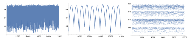
Figure 3. Fluctuation of $c_{\zeta}(H)$

Euler function twisted by Dirichlet character

Let $F(s)=L(s,\psi)$, where $\psi$ is a real non-principal Dirichlet character modulo $q$. Taking into consideration,

$$\varphi(n,\psi)=n\prod_{p\mid n}\left(1-\frac{\psi(p)}{p}\right).$$

Kaczorowski and Wiertelak [14] read up on the Omega results of $\sum_{n\leq x}\varphi(n,\psi)-\frac{x^{2}}{2L(2,\psi)}$ and further Kaczorowski [13] also studied the mean square for the same. As a consequence of Theorem 1.5, we derive the following variance for $\frac{\varphi(n,\psi)}{n}$ in the short intervals.

Corollary 1.7.

Let $\epsilon>0$ be given. For $2\leq H\leq X^{1-\epsilon}$, we have

$$\frac{1}{X}\int_{X}^{2X}\bigg{|}\sum_{x<n\leq x+H}\frac{\varphi(n,\psi)}{n}-\frac{H}{L(2,\psi)}\bigg{|}^{2}dx=c(H)+O(H^{-\epsilon}),$$

where

$$c(H)=\sum_{\begin{subarray}{c}d=1\\ (d,q)=1\end{subarray}}^{\infty}\frac{\mu^{2}(d)}{d^{2}}\prod_{p\nmid d}\left(1+\frac{2\psi(p)}{p^{2}}\right)\left(\left\{\frac{H}{d}\right\}-\left\{\frac{H}{d}\right\}^{2}\right).$$

Schemmel’s totient in short intervals

For any $m\geq 1$, the Schemmel’s totient function $S_{m}(n)$ was introduced by Schemmel in [29], which counts the number of sets of $m$ consecutive integers each less than $n$ and relatively prime to $n$. The function $S_{m}(n)$ has a product representation of the form

$$S_{m}(n)=\begin{cases}0&\mbox{ if }\,P^{-}(n)\leq m,\\ n\prod_{p\mid n}\left(1-\frac{m}{p}\right)=n\sum_{\begin{subarray}{c}d\mid n\end{subarray}}\frac{\mu(d)m^{w(d)}}{d}&\mbox{ if }\,P^{-}(n)>m.\end{cases}$$

The following corollary is a consequence of Remark 5.

Corollary 1.8 (Sieving by the primes $\leq m$).

Let $\epsilon>0$ be given. Assume that $P(m)=\prod_{p\leq m}p$. Then for $H\leq X^{1-\epsilon}$, we have

$$\frac{1}{X}\int_{X}^{2X}\bigg{|}\sum_{\begin{subarray}{c}x<n\leq x+H\\ \left(n,P(m)\right)=1\end{subarray}}\frac{S_{m}(n)}{n}-\prod_{p\leq m}\left(1-\frac{1}{p}\right)\prod_{p\nmid P(m)}\left(1-\frac{m}{p^{2}}\right)\,H\bigg{|}^{2}dx=c_{m}(H)+O(H^{-\epsilon}),$$

where

$$c_{m}(H)=\sum_{\begin{subarray}{c}d=1\\ (d,P(m))=1\end{subarray}}^{\infty}\frac{\mu^{2}(d)m^{2\omega(d)}}{d^{2}}\prod_{p\nmid d}\left(1-\frac{2m}{p^{2}}\right)\sum_{t\mid P(m)}\prod_{\begin{subarray}{c}p\mid P(m)\\ p\nmid t\end{subarray}}\left(1-\frac{2}{p}\right)\left(\left\{\frac{H}{td}\right\}-\left\{\frac{H}{td}\right\}^{2}\right).$$

There are many generalizations connected to the Euler totient function; namely, Jordan totient function, Klee’s totient function and several others can be found in [28] (see Chapter 3) and further in [27]. We can similarly obtain the variance of these functions using Theorem 1.5.

1.3.2. $k$-free integers

It is well known that the $k$-free integers have density $\frac{1}{\zeta(k)}$ in $\mathbb{N}$. We denote $E_{k}(x)$ by

$$E_{k}(x)=\sum_{n\leq x}\mu_{k}(n)-\frac{x}{\zeta(k)}.$$

It is easy to prove that $E_{k}(x)=O\left(x^{\frac{1}{k}}\right)$. The best known upper bound, due to Walfisz [35], employed the sharpest known zero-free region of the Riemann zeta function to show that

$$E_{k}(x)=O\left(x^{1/k}\exp(-ck^{-8/5}(\log x)^{3/5}(\log\log x)^{1/5}\right)$$

for an absolute positive constant $c$. This bound has seen several improvements for each $k$, under the assumption of the Riemann hypothesis (see for instance [3, 9, 17, 18]). It is widely conjectured that

(1.9) $$E_{k}(x)=O\left(x^{\frac{1}{2k}+\epsilon}\right).$$

In fact, if $E_{k}(x)=O\left(x^{\frac{1}{2k}+\epsilon}\right)$ then it is straightforward to show that the Riemann hypothesis follows, as well as the simplicity of the zeros of the Riemann zeta function on the critical line. Recently, Mossinghoff et al. [25] showed that $E_{k}(x)/x^{1/2k}<-3$ infinitely often and $E_{k}(x)/x^{1/2k}>3$ infinitely often, for $k=2,3,4$ and $5$. They also studied the ratio $E_{k}(x)/x^{1/2k}$ for sufficiently large values of $k$. Analogous to (1.9), one can conjecture that for any given $\epsilon>0$, uniformly in $x^{\epsilon}\leq H\leq x$,

(1.10) $$\sum_{x<n\leq x+H}\mu_{k}(n)=\frac{H}{\zeta(k)}+O\left(H^{\frac{1}{2k}+\epsilon}\right).$$

When $H$ is close to $x^{\epsilon}$, there are no asymptotic estimates are known (see the work of Tolev [33]). For large $H$, say $H=x$, estimating the sum in (1.10) asymptotically is straightforward, but obtaining an error term $O\left(H^{\frac{1}{2k}+\epsilon}\right)$ is an open problem, even conditionally on the Riemann Hypothesis.

In the matter of $k=2$, Gorodetsky et al. [7] extended the work of Hall [11] and established (1.10) on average with $\epsilon$ removed. Recently, Gorodetsky, Mangerel and Rodgers [8] computed moments for $k$-free integers (more generally $B$-free numbers) to study their Gaussian distribution. In particular, second moment (see Proposition 1.7 and Proposition 1.9) gives an error term of size $O(H^{\frac{1}{k}-\epsilon})$ if $H\leq X^{\frac{k(k-1)}{(k+1)(2k-1)}-\epsilon}$. As an application of Theorem 1.3, the following corollary improved the above mentioned result of [8] when $k\geq 3$ and also the range of $\epsilon$ compared to Theorem $1$ of [7] for the square-free numbers.

For $s\in\mathbb{C}\setminus\{1\}$, the function $\chi$ is defined by

(1.11) $$\chi(s)=2^{s}\pi^{s-1}\Gamma(1-s)\sin(\pi s/2),$$

and it appears in the functional equation of Riemann zeta function i.e., $\zeta(s)=\chi(s)\zeta(1-s)$.

Corollary 1.9.

Let $X\geq 1$ be sufficiently large and $\nu,e(k,0)$ and $g(k)$ be defined by (1.3)- (1.4). Let $\epsilon\in(0,\frac{3}{10})$ be given. For $2\leq H\leq X^{e(k,0)-\epsilon}$, we have

$$\frac{1}{X}\int_{X}^{2X}\bigg{|}\sum_{x<n\leq x+H}\mu_{k}(n)-\frac{H}{\zeta(k)}\bigg{|}^{2}dx=c_{k}H^{\frac{1}{k}}+O\left(H^{\frac{1}{k}-\frac{\epsilon}{3(k+1)}}\right),$$

where

$$c_{k}=-\frac{1}{2\pi^{2}}\chi{\Big{(}\frac{k+1}{k}\Big{)}}\zeta{\Big{(}2-\frac{1}{k}\Big{)}}\prod_{p}\bigg{(}1-\frac{1}{p^{2}}-\frac{2(p-1)}{p^{k+1}}\bigg{)}.$$

Assuming the Lindelöf Hypothesis, the above estimate holds for the wider range $H\leq X^{g(k)-\epsilon}$.

Remark 6.

We significantly improve the length of short intervals when $k\geq 3$; for example, $e(3,0)\approx 0.60537,\,e(4,0)\approx 0.65797,\,\ldots,e(10^{5},0)\approx 0.77346$ compare to the exponent $e(3,0)\approx 0.3,e(4,0)\approx 0.34286,\ldots,e(10^{5},0)\approx 0.49999$ in [8]. Under the Lindelöf hypothesis, we further stretch the exponents as $g(k)$; namely, $g(3)\approx 0.7182,g(4)\approx 0.7355,\ldots,g(10^{5})\approx 0.77346$. Unconditionally exponents are same as under the Lindelöf hypothesis upto some decimal places for sufficiently large values of $k$.

1.3.3. Möbius function of order $k$

Let $r\geq 1$ and $k\geq 2$. The Möbius function of order $k$, introduced by T. M. Apostol [1], which is defined by:

$$\widehat{\mu}_{k}(n)=\begin{cases}1&\mbox{ if }\,n=1,\\ 0&\mbox{ if }\,p^{k+1}\mid n\,\text{ for some prime }p,\\ (-1)^{r}&\mbox{ if }\,n=p_{1}^{k}\ldots p_{r}^{k}\prod_{i>r}p_{i}^{a_{i}},\,0\leq a_{i}<k,\\ 1&\mbox{ otherwise}.\end{cases}$$

Specializing to the case $k=1$ gives the classical Möbius function. To study behaviour of the function $\widehat{\mu}_{k}(n)$ on average, it is enough to study the following mean value:

$$F_{r}(x):=\sum_{n\leq x}\widehat{\mu}_{k-1}(n)\widehat{\mu}_{k-1}(r^{k-1}n)=\mu(r)\sum_{\begin{subarray}{c}n\leq x\\ (n,r)=1\end{subarray}}\mu_{k}(n).$$

Note that,

$$\sum_{n\leq x}\widehat{\mu}_{k}(n)=\sum_{r\leq x^{1/k}}F(x/r^{k}).$$

The following corollary is a direct consequence of Theorem 1.3.

Corollary 1.10.

Let $\epsilon,\nu,e(k,0)$ and $g(k)$ be as in Corollary 1.9. Assume that $H\leq X^{e(k,0)-\epsilon}$. Then

$$\frac{1}{X}\int_{X}^{2X}\bigg{|}F_{r}(x+H)-F_{r}(x)-\frac{\varphi(r)r^{k-1}\mu(r)}{\zeta(k)J_{k}(r)}H\bigg{|}^{2}dx=c_{k,r}H^{\frac{1}{k}}+O\left(H^{\frac{1}{k}-\frac{\epsilon}{3(k+1)}}\right),$$

where

$$c_{k,r}=-\frac{\mu^{2}(r)}{2\pi^{2}}\chi{\Big{(}\frac{k+1}{k}\Big{)}}\zeta{\Big{(}2-\frac{1}{k}\Big{)}}\prod_{p}\bigg{(}1-\frac{1}{p^{2}}-\frac{2(p-1)}{p^{k+1}}\bigg{)}\prod_{p\mid r}\left(1-\frac{2}{p^{k}}+\frac{1}{p}\right)^{-1}.$$

Assuming the Lindelöf Hypothesis, the above estimate holds for the extended range $H\leq X^{g(k)-\epsilon}$.

As an another application of Theorem 1.3, we obtain the variance of an arithmetical function associated with counting prime factors.

Corollary 1.11.

Let $\epsilon,\nu,e(k,0)$ and $g(k)$ be as in Corollary 1.9. For $2\leq H\leq X^{e(k,0)-\epsilon}$, we have

$$\frac{1}{X}\int_{X}^{2X}\bigg{|}\sum_{x<n\leq x+H}(-1)^{\#\{p:\,p^{k}\mid n\}}-\prod_{p}\left(1-\frac{2}{p^{k}}\right)H\bigg{|}^{2}dx=c_{k}H^{\frac{1}{k}}P_{3}(\log H)+O\left(H^{\frac{1}{k}-\frac{\epsilon}{3(k+1)}}\right),$$

where

$$c_{k}=-\frac{1}{24\pi^{2}}\chi{\Big{(}\frac{k+1}{k}\Big{)}}\zeta{\Big{(}2-\frac{1}{k}\Big{)}}\prod_{p}\left(1-\frac{4}{p^{k}}+\frac{4}{p}\right)\left(1-\frac{1}{p}\right)^{4}.$$

Assuming the Lindelöf Hypothesis, the above estimate holds for the wider range $H\leq X^{g(k)-\epsilon}$.

1.3.4. Generalized sum of divisor function

Let $\alpha\in\mathbb{R}$. The generalized sum of divisor function $\sigma_{\alpha}(n)$ is denoted the $n$-th coefficient of the Dirichlet series $\zeta(s)\zeta(s-\alpha)$; i.e.,

$$\sigma_{\alpha}(n)=\sum_{d\mid n}d^{\alpha}.$$

Chowla [5] first studied the variance of $\sigma_{\alpha}(n)$ and proved that for $-1<\alpha<-\frac{1}{2}$,

$$\frac{1}{X}\int_{X}^{2X}\bigg{|}\sum_{n\leq x}\sigma_{\alpha}(n)-\zeta(1-\alpha)x\bigg{|}^{2}dx=c_{1}+O\left(X^{1/2+\alpha}\log X\right),$$

for some explicit constant $c_{1}$ depends on $\alpha$. Afterward, Lau [16] derived an $\Omega_{\pm}$-result. In short intervals, Kiuchi and Tanigawa [15] obtained that for $-1<\alpha<-\frac{1}{2}$ and $H\ll X^{1/2}$,

(1.12) $$\frac{1}{X}\int_{X}^{2X}\bigg{|}\sum_{x<n\leq x+H}\sigma_{\alpha}(n)-\zeta(1-\alpha)H\bigg{|}^{2}dx\ll X^{\epsilon}.$$

Our next corollary yields a notable improvement of the above result of Kiuchi and Tanigawa in a wide range of $H$ and $\alpha$. It is an application of Theorem 1.5.

Corollary 1.12.

Let $\epsilon>0$ be given. Then for $2\leq H\leq{X^{\frac{29}{113+84\alpha}-\epsilon}}$, whenever $\alpha\in(-1,-1/2)$ and $2\leq H\leq X^{1-\epsilon},$ when $\alpha\in(-2,-1]$, we have

$$\frac{1}{X}\int_{X}^{2X}\bigg{|}\sum_{x<n\leq x+H}\sigma_{\alpha}(n)-\zeta(1-\alpha)H\bigg{|}^{2}dx=c(H)+O(H^{-\epsilon}),$$

where

$$c(H)=\frac{\zeta(1-\alpha)^{2}}{\zeta(2-2\alpha)}\sum_{d=1}^{\infty}d^{2\alpha}\left(\left\{\ \frac{H}{d}\right\}-\left\{\frac{H}{d}\right\}^{2}\right).$$

Assuming Lindelöf hypothesis, we have the extended range $H\leq X^{\frac{1}{3+2\alpha}-\epsilon}$ for $\alpha\in(-1,-1/2)$.

Remark 7.

First of all, Corollary 1.12 gives an asymptotic formula with a constant to its main term which improves the weaker bound in (1.12). Also we provide a better range of $H$ for $\alpha\in(-1,-0.66]$ which breaks the $\frac{1}{2}$-barrier. For instance, if $\alpha=\frac{3}{4}$ then the exponent is $0.58$ and for $\alpha=0.99$ it is approximately $0.97$.

2. Parameters used in main theorems

In this section, we introduce several functions which are used in the statement of main theorems.

For the range $\alpha\in[0,1/2)$

Assume that $\beta\in\mathbb{Z}\setminus\{0\}$ and $k\geq 2$. For $s\in\mathbb{C}$, we define

(2.1) $$B(s):=\prod_{p}\left(1+\frac{2h(p)}{p^{k}}+\frac{h(p)^{2}}{p^{k+ks}}\right)\left(1-\frac{1}{p^{k+ks+2\alpha}}\right)^{\beta^{2}}$$

and

(2.2) $$D(s):=\prod_{p}\left(1-\frac{h(p)^{2}}{p^{k+ks}}\right)^{-1}\left(1-\frac{1}{p^{k+ks+2\alpha}}\right)^{\beta^{2}}\left(1-\frac{h(p)^{2}}{p^{2k}}\right)\left(1-\frac{h(p)}{p^{k}}\right)^{-2}.$$

Recall the function $\chi(s)$ from (1.11). Let us consider

(2.5) $$c_{h,k}= \left\{\begin{array}[c]{ll}-\frac{1}{4\pi^{2}(\beta^{2}-1)!}B\left(\frac{1-2\alpha-k}{k}\right)\chi(\frac{k+1-2\alpha}{k})\zeta\left(2-\frac{1-2\alpha}{k}\right)&\text{ if }h\in\mathcal{M}_{\alpha}^{\mu},\\ -\frac{1}{4\pi^{2}(\beta^{2}-1)!}D\left(\frac{1-2\alpha-k}{k}\right)\chi(\frac{k+1-2\alpha}{k})\zeta\left(2-\frac{1-2\alpha}{k}\right)&\,\text{if }h\in\mathcal{G}_{\alpha},\end{array}\right.$$

and

(2.8) $$P_{t}(x)= \left\{\begin{array}[c]{ll}\sum_{\begin{subarray}{c}r+l+m+n=t\\ r,l,m,n\geq 0\end{subarray}}\Big{(}\frac{B^{(r)}}{B}\cdot\frac{G_{k}^{(l)}}{G_{k}}\cdot\frac{\chi^{(m)}}{\chi}\Big{)}\left(\frac{1-2\alpha-k}{2\pi ik}\right)x^{n}&\text{ if }h\in\mathcal{M}_{\alpha}^{\mu},\\ \sum_{\begin{subarray}{c}r+l+m+n=t\\ r,l,m,n\geq 0\end{subarray}}\Big{(}\frac{D^{(r)}}{D}\cdot\frac{G_{k}^{(l)}}{G_{k}}\cdot\frac{\chi^{(m)}}{\chi}\Big{)}\left(\frac{1-2\alpha-k}{2\pi ik}\right)x^{n}&\,\text{if }h\in\mathcal{G}_{\alpha},\end{array}\right.$$

where $P_{t}(x)$ is a monic polynomial in $x$ of degree $t$, $(f\cdot g\cdot h)(x):=f(x)g(x)h(x)$, and

(2.9) $$G_{k}(s):=\zeta(1-s)\zeta^{\beta^{2}}(k+ks+2\alpha)\left(s-\frac{1-2\alpha-k}{k}\right)^{\beta^{2}}.$$

We also define

(2.10) $$\lambda_{j,\alpha}(\beta^{2}):=\frac{1}{\Gamma(\beta^{2}-j)}\sum_{h+i=j}\frac{1}{i!h!}L_{\alpha}^{(h)}(1)\gamma_{i}(\beta^{2})$$

and $\gamma_{i}$’s are given by the Taylor series expansion

(2.11) $$\frac{1}{z}((z-1)\zeta(z))^{\beta^{2}}=\sum_{j\geq 0}\frac{1}{j!}\gamma_{j}(\beta^{2})(z-1)^{j},$$

where

$$L_{\alpha}(z):=\begin{cases}z\,\zeta\left(2-\frac{z-2\alpha}{k}\right)B\left(-1+\frac{z-2\alpha}{k}\right)\chi\big{(}\frac{-1+(z-2\alpha)/k}{2\pi i}\big{)}\,&\text{ if }h\in\mathcal{M}_{\alpha}^{\mu},\\ z\,\zeta\left(2-\frac{z-2\alpha}{k}\right)D\left(-1+\frac{z-2\alpha}{k}\right)\chi\big{(}\frac{-1+(z-2\alpha)/k}{2\pi i}\big{)}&\,\text{if }h\in\mathcal{G}_{\alpha}.\end{cases}$$

For the range $\alpha\in(1/2,2)$

We define the constant depends on $H$ as

(2.12) $$c_{h,k}(H):=\begin{cases}\displaystyle\sum_{d=1}^{\infty}h^{2}(d)\prod_{p\nmid d}\left(1+\frac{2h(p)}{p^{k}}\right)\bigg{(}\left\{\frac{H}{d^{k}}\right\}-\left\{\frac{H}{d^{k}}\right\}^{2}\bigg{)}&\mbox{ if }h\in\mathcal{M}_{\alpha}^{\mu},\\ \displaystyle\bigg{(}\prod_{p}\frac{p^{k}+h(p)}{p^{k}-h(p)}\bigg{)}\sum_{d=1}^{\infty}h^{2}(d)\bigg{(}\left\{\frac{H}{d^{k}}\right\}-\left\{\frac{H}{d^{k}}\right\}^{2}\bigg{)}&\mbox{ if }h\in\mathcal{G}_{\alpha}.\end{cases}$$

3. Preparation for the proof of Theorem 1.3 and Theorem 1.5

To prove Theorem 1.3 and Theorem 1.5 we state main propositions which has been proven in Section 5, 6 and 7. The first two propositions give us an asymptotic formula for the variance of a random variable up to a parameter $z$ while the third proposition estimates the upper bound of the same random variable beyond $z$. To serve our purpose we denote such restricted variance by $\mathcal{J}_{k,z}(H;h)$ and $\mathcal{K}_{k,z}(H;h)$ respectively; i.e., for sufficiently large $X\geq 1$,

(3.1) $$\mathcal{J}_{k,z}(H;h):=\frac{1}{X}\int_{X}^{2X}\bigg{|}\sum_{\begin{subarray}{c}x<nd^{k}\leq x+H\\ d^{k}\leq z\end{subarray}}h(d)-H\sum_{d^{k}\leq z}\frac{h(d)}{d^{k}}\bigg{|}^{2}dx,$$

(3.2) $$\mathcal{K}_{k,z}(H;h):=\frac{1}{X}\int_{X}^{2X}\bigg{|}\sum_{\begin{subarray}{c}x<nd^{k}\leq x+H\\ d^{k}>z\end{subarray}}h(d)-H\sum_{d^{k}>z}\frac{h(d)}{d^{k}}\bigg{|}^{2}dx.$$

Proposition 3.1.

Let $f\in\mathcal{F}_{\alpha,\beta,k}$ with $\beta\in\mathbb{Z}\setminus\{0\}$ and $0\leq\alpha<\frac{1}{2}$. Let $0<\epsilon<\frac{1-2\alpha}{2(\lceil\beta^{2}/12\rceil+4)}$ be given. Case 1: Assume $k=2$ and $X^{\epsilon}\leq H\leq X^{\frac{2+\alpha}{3+2\alpha}-\epsilon}$. For a parameter $H^{1+\epsilon}\leq z\leq\min\Big{\{}X^{\frac{1}{1-\alpha}}H^{-\frac{1+2\alpha}{2-2\alpha}-\epsilon},H^{\frac{1-2\alpha}{2-2\alpha}-\epsilon}X^{\frac{1}{2-2\alpha}}\Big{\}},$ we obtain

$$\mathcal{J}_{2,z}(H;h)=c_{h,2}H^{\frac{1-2\alpha}{2}}P_{\beta^{2}-1}(\log H)+O\left(H^{\frac{1-2\alpha}{2}-\frac{\epsilon}{5}}\right).$$

Case 2: For $k\geq 3$ and $H^{1+\epsilon}\leq z\leq\min\Big{\{}X^{\frac{2}{\nu(2-\alpha)}}H^{\frac{1-2\alpha}{\nu(2-\alpha)}-\epsilon},X^{\frac{\nu}{2(\nu-\alpha)}}H^{\frac{1-2\alpha}{2(\nu-\alpha)}-\epsilon},X^{\frac{2(k-\nu)}{(4-\nu)k-2\nu}-\epsilon}\Big{\}}$,

$$\mathcal{J}_{k,z}(H;h)=c_{h,k}H^{\frac{1-2\alpha}{k}}P_{\beta^{2}-1}(\log H)+O\left(H^{\frac{1-2\alpha}{k}-\frac{\epsilon}{k+1}}\right),$$

where $\nu,c_{h,k}$ and $P_{\beta^{2}-1}(\log H)$ are as in (1.3), (2.5) and (2.8) respectively.

Proposition 3.2.

Let $f\in\mathcal{F}_{\alpha,\beta,k}$ with $\beta\in\mathbb{Z}\setminus\{0\}$ and $k\geq 1$. Let $\epsilon>0$ be given and $\epsilon_{\alpha,k}>0$ depends on $\epsilon,\alpha$ and $k$. If $\frac{1}{2}<\alpha<1$ then we have

$$\mathcal{J}_{k,z}(H;h)=c_{h,k}(H)+O\left(H^{-\epsilon_{\alpha,k}}\right),$$

provided that

$$z\leq\begin{cases}X^{\frac{1}{2(1-\alpha)}}H^{-\frac{1}{2(1-\alpha)}-\epsilon}&\mbox{ if }k=1,\\ \min\big{\{}X^{\frac{1}{1-\alpha}}H^{-\frac{1}{1-\alpha}-\epsilon},X^{\frac{1}{2-2\alpha}}H^{-\epsilon}\big{\}}&\mbox{ if }H\leq X^{\frac{2+\alpha}{4}-\epsilon}\text{ and }k=2,\\ \min\big{\{}X^{\frac{2}{\nu(2-\alpha)}-\epsilon},X^{\frac{\nu}{2(\nu-\alpha)}-\epsilon},X^{\frac{2(k-\nu)}{(4-\nu)k-2\nu}-\epsilon}\big{\}}&\mbox{ if }k\geq 3.\end{cases}$$

Suppose that $1\leq\alpha<2$ and $z\leq 2X$. In this case, the above estimate holds whenever $H\leq X^{1-\epsilon}$ if $k\in\mathbb{N}\setminus\{2\}$ and $H\leq X^{\frac{2+\alpha}{4}-\epsilon}$ if $k=2$.

Proposition 3.3.

Let $f\in\mathcal{F}_{\alpha,\beta,k}$ with $\beta\in\mathbb{C}\setminus\{0\}$ and $\epsilon>0$ be given. Assume that $0\leq\alpha<\frac{1}{2}$, $k\geq 2$ and $X^{\epsilon}\leq H\leq X^{\frac{29k}{29k+42}-\epsilon}$. If $z\geq H^{\frac{k+2\alpha-1}{k+2\alpha-5/4}+\epsilon}$ then we have

$$\mathcal{K}_{k,z}(H;h)\ll H^{\frac{1-2\alpha}{k}-\frac{\epsilon}{3}}.$$

Under the Lindelöf hypothesis, the claim holds with $X^{\epsilon}\leq H\leq X^{\frac{k}{k+1}-\epsilon}$ and $z\geq H^{1+\epsilon}$.
Assume that $\frac{1}{2}<\alpha<1$, $k\geq 1$, and $X^{\epsilon}\leq H\leq X^{\frac{29k}{29k+84(1-\alpha)}-\epsilon}$. If $z\geq H^{\frac{k}{k+2\alpha-5/4}+\epsilon}$ then

$$\mathcal{K}_{k,z}(H;h)\ll H^{-\frac{\epsilon}{3}}.$$

Under the Lindelöf hypothesis, we have extended range $X^{\epsilon}\leq H\leq X^{\frac{k}{k-2\alpha+2}-\epsilon}$ and $z\geq H^{1+\epsilon}$.

Remark 8.

Observe that if $\frac{1}{2}<\alpha<1$ and $k=1,2$ then the exponents of short intervals in Theorem 1.5 depend on the range $H\leq X^{\frac{29k}{29k+84(1-\alpha)}-\epsilon}$ of Proposition 3.3. Here we used Bourgain’s bound instead of standard sub-convexity bound for Riemann zeta function to get better exponents.

Now we establish the discrete variance in short intervals. For sufficiently large $X$, let us define the discrete variance of $f\in\mathcal{F}_{\alpha,\beta,k}$ with $\beta\in\mathbb{Z}\setminus\{0\}$ as follows:

$$\operatorname{Var}_{\mathcal{D}}(\mathcal{F}_{\alpha,\beta,k}):=\frac{1}{X}\sum_{n\leq X}\left(\sum_{j=1}^{H}f(n+j)-\widetilde{c}_{h,k}H\right)^{2}.$$

Here we define the exponent of short intervals as

(3.3) $$\theta(k,\alpha):=\begin{cases}\frac{k(k+\alpha-1)}{(k-\alpha+1)(2k+2\alpha-1)}&\mbox{ if }\quad 0\leq\alpha<\frac{1}{2},\\ \frac{k+\alpha-1}{2(k-\alpha+1)}&\mbox{ if }\quad\frac{1}{2}<\alpha<2.\end{cases}$$

Proposition 3.4.

Assume that $0<\epsilon<\frac{3(1-2\alpha)}{k(k\beta^{2}+3)}$ with $\alpha\in[0,1/2)$ and $k\geq 2$. Let $2\leq H\leq X^{\theta(k,\alpha)-\epsilon}$. Then we have

$$\operatorname{Var}_{\mathcal{D}}(\mathcal{F}_{\alpha,\beta,k})=c_{h,k}H^{\frac{1-2\alpha}{k}}P_{\beta^{2}-1}(\log H)+O\left(H^{\frac{1-2\alpha}{k}-\epsilon}\right),$$

where $c_{h,k}$ and $P_{\beta^{2}-1}(\log H)$ are defined by (2.5) and (2.8) respectively.

Remark 9.

Observe that Proposition 3.4 recovers the main result of Avdeeva [2] and Proposition $1.7$ of [8] for some specific cases of $B$-free integers (for example, $k$-free integers).

Proposition 3.5.

Let $\epsilon>0$ be given and $1/2<\alpha<2$. For $k\geq 1$ and $2\leq H\leq X^{\theta(k,\alpha)-\epsilon}$,

$$\operatorname{Var}_{\mathcal{D}}(\mathcal{F}_{\alpha,\beta,k})=c_{h,k}(H)+O(H^{-\epsilon}).$$

Remark 10.

Recall $e(k,\alpha)$ from (1.3). We see that in the case of continuous variance $X^{\epsilon}\leq H\leq X^{e(k,\alpha)-\epsilon}$, whereas in the discrete case $2\leq H\leq X^{\theta(k,\alpha)-\epsilon}$. Note that $\theta(k,\alpha)$ is bounded by $\frac{1}{2}$ and it seems very difficult to break $\frac{1}{2}$-barrier through discrete process. Also $e(k,\alpha)$ is much bigger than $\theta(k,\alpha)$ which has been drawn in Figure 4.

Remark 11.

The point $\alpha=\frac{1}{2}$ is called here the critical or stationary point. It seems extremely tricky to separate out main term (which is a constant) with a permeable error term using complex analysis technique (see Lemma 7.2).

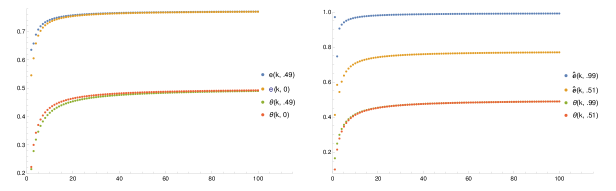
Figure 4. Comparison between exponents of continuous and discrete variance

4. Proof of Theorems

In this section, we prove our main theorems by making use of propositions from Section 3.

Proof of Theorem 1.3.

First, we consider the case when $H>X^{\epsilon}$. For any $f\in\mathcal{F}_{\alpha,\beta,k}$, we have

(4.1) $$\sum_{x<n\leq x+H}f(n)=\sum_{x<ad^{k}\leq x+H}h(d)=\sum_{\begin{subarray}{c}x<ad^{k}\leq x+H\\ d^{k}\leq z\end{subarray}}h(d)+\sum_{\begin{subarray}{c}x<ad^{k}\leq x+H\\ d^{k}>z\end{subarray}}h(d),$$

where $z$ will be chosen later. Let us denote the integral $\mathcal{J}_{k,z}(H;h)$ by $I_{k1}$ and $\mathcal{K}_{k,z}(H;h)$ by $I_{k2}$. Using Cauchy-Schwarz inequality and (4.1),

$$I_{k}:=\frac{1}{X}\int_{X}^{2X}\bigg{|}\sum_{x<n\leq x+H}f(n)-H\sum_{d^{k}\leq 2X}\frac{h(d)}{d^{k}}\bigg{|}^{2}dx=I_{k1}+O\left(I_{k2}+\sqrt{I_{k1}I_{k2}}\right).$$

The class $\mathcal{F}_{\alpha,\beta,2}$

For $X^{\epsilon}<H\leq X^{\frac{2(3+8\alpha)}{11(1+2\alpha)}-\epsilon}$ we take $z=\min\Big{\{}X^{\frac{1}{1-\alpha}}H^{-\frac{1+2\alpha}{2-2\alpha}-\epsilon},H^{\frac{1-2\alpha}{2-2\alpha}-\epsilon}X^{\frac{1}{2-2\alpha}}\Big{\}}$. The range of $H$ gives us $z\geq H^{\frac{4(1+2\alpha)}{3+8\alpha}+\epsilon}$. Using Proposition 3.1 and Proposition 3.3, we deduce

$$I_{2}=c_{h,2}H^{\frac{1-2\alpha}{2}}P_{\beta^{2}-1}(\log H)+O\left(H^{\frac{1-2\alpha}{2}-\frac{\epsilon}{8}}\right).$$

For the class $\mathcal{F}_{\alpha,\beta,k}$ with $k\geq 3$.

Recall $\nu$ and $e(k,\alpha)$ from (1.3) and (1.4) respectively. Assume that $X^{\epsilon}<H\leq X^{e(k,\alpha)-3\epsilon}$. Consider

$$z=\min\Big{\{}X^{\frac{2}{\nu(2-\alpha)}}H^{\frac{1-2\alpha}{\nu(2-\alpha)}-\epsilon},X^{\frac{\nu}{2(\nu-\alpha)}}H^{\frac{1-2\alpha}{2(\nu-\alpha)}-\epsilon},X^{\frac{2(k-\nu)}{(4-\nu)k-2\nu}-\epsilon}\Big{\}}.$$

Therefore, it is easy to see that $z\geq H^{\frac{k+2\alpha-1}{k+2\alpha-5/4}+\epsilon}$. This gives whenever $1<\nu\leq 2$,

$$H\leq X^{\min\big{\{}f_{1}(\nu),\,f_{2}(\nu),\,f_{3}(\nu)\big{\}}},$$

where

$$f_{1}(\nu)=\frac{2(k+2\alpha-5/4)}{\nu(2-\alpha)(k+2\alpha-1)-(1-2\alpha)(k+2\alpha-5/4)},$$

$$f_{2}(\nu)=\frac{\nu(k+2\alpha-5/4)}{2(\nu-\alpha)(k+2\alpha-1)-(1-2\alpha)(k+2\alpha-5/4)},$$

$$f_{3}(\nu)=\frac{2(k-\nu)(k+2\alpha-5/4)}{(4k-(k+2)\nu)(k+2\alpha-1)}.$$

One can check that $f_{1}(\nu)>f_{2}(\nu)$, since $1.34<\nu\leq 2$. So it is enough to consider the minimum of $f_{2}(\nu)$ and $f_{3}(\nu)$. Since $f_{2}$ is a decreasing and $f_{3}$ is an increasing function then they meet at $\nu$, which is given by (1.3).

Using Proposition 3.1 and Proposition 3.3 and rescaling $3\epsilon$ to $\epsilon$, we obtain

$$I_{k}=c_{h,k}H^{\frac{1-2\alpha}{k}}P_{\beta^{2}-1}(\log H)+O\left(H^{\frac{1-2\alpha}{k}-\frac{\epsilon}{3(k+1)}}\right).$$

It remains to estimate the tail part of $\operatorname{Var}(\mathcal{F}_{\alpha,\beta,k})$. Observe that

$$\sum_{d^{k}\geq X}\frac{h(d)}{d^{k}}\ll X^{-\frac{k+\alpha-1-\epsilon_{1}}{k}}.$$

Using this estimate we have

(4.2) $$E_{k}:=\frac{1}{X}\int_{X}^{2X}\bigg{|}H\sum_{d^{k}\geq X}\frac{h(d)}{d^{k}}\bigg{|}^{2}dx\ll H^{2}X^{-\frac{2(k+\alpha-1-\epsilon_{1})}{k}}.$$

By Cauchy-Schwarz inequality,

$$\operatorname{Var}(\mathcal{F}_{\alpha,\beta,k})=I_{k}+O\left(E_{k}+\sqrt{I_{k}\cdot E_{k}}\right),$$

The estimate of $I_{k}$ and $E_{k}$ yields

$$\sqrt{I_{k}\cdot E_{k}}\ll HX^{-\frac{k+\alpha-1-\epsilon_{1}}{k}}H^{\frac{1-2\alpha}{2k}}(\log H)^{\beta^{2}-1}\ll H^{\frac{1-2\alpha}{k}-\epsilon}$$

provided that $H\leq X^{\frac{2(k+\alpha-1)}{2k+2\alpha-1}-\epsilon}$. Inserting the above estimates in $\operatorname{Var}(\mathcal{F}_{\alpha,\beta,k})$ completes the proof whenever $H>X^{\epsilon}$.

Now consider that $2\leq H\leq X^{\epsilon}$. Note that the difference between continuous and discrete variance is small of size $O(H/X)$. Hence, Theorem 1.3 follows from Proposition 3.4. ∎

Proof of Theorem 1.5.

We first assume that $H>X^{\epsilon}$. Let $f\in\mathcal{F}_{\alpha,\beta,k}$ with $1/2<\alpha<2$.

Case 1.

Let $1\leq\alpha<2$. Recall $\mathcal{J}_{k,z}(H;h)$ from Proposition 3.2. For $z=2X$, we have

$$\mathcal{J}_{k,2X}(H;h)=\begin{cases}c_{h,2}(H)+O(H^{-\epsilon_{\alpha,k}})&\mbox{ if }H\leq X^{\frac{2+\alpha}{4}-\epsilon},\,k=2,\\ c_{h,k}(H)+O(H^{-\epsilon_{\alpha,k}})&\mbox{ if }H\leq X^{1-\epsilon},\,k\neq 2.\end{cases}$$

Applying Cauchy-Schwarz inequality,

$$\operatorname{Var}(\mathcal{F}_{\alpha,\beta,k})=\mathcal{J}_{k,2X}(H;h)+O\left(E_{k}+\sqrt{\mathcal{J}_{k,2X}(H;h)\times E_{k}}\right),$$

where $E_{k}$ is estimated in (4.2). Since $H\ll X^{1-\epsilon}$, the above error term is of size $O(H^{-\epsilon_{\alpha,k}})$.

Case 2.

Assume that $\frac{1}{2}<\alpha<1$. The proof of this case proceeds along the arguments of Case 1 and Theorem 1.3. In addition, we use Proposition 3.2 and Proposition 3.3 to conclude the proof.

For $2\leq H\leq X^{\epsilon}$, Theorem 1.5 follows from Proposition 3.5. ∎

Proof of Theorem 1.4.

Let us consider that $H>X^{\epsilon}$. Note that Lemma 5.4 and Lemma 5.7 is also valid for $\beta\in\mathbb{C}$. Combining these Lemmas together with Lemma 5.3, Proposition 3.3 and following the proof of Theorem 1.3, we conclude the proof.

Next suppose that $2\leq H\leq X^{\epsilon}$. For $\beta\in\mathbb{C}$ we can obtain an analogue of Proposition 3.4 with a weaker error term (which matches our asymptotic formula) by a modification of its proof. Indeed, we easily carry out the proof of Proposition 3.4 to reach the integral (7.3) where complex $\beta$ would not be effective. To compute (7.3) we follow the method in proof of Lemma 5.3 and finishes the proof. ∎

5. Proof of Proposition 3.1 and Proposition 3.2

We use the Fourier series of Bernoulli’s polynomial to get the following standard formula.

Lemma 5.1.

For a real number $x$, we have

$$\sum_{n=1}^{\infty}\frac{\cos{(2\pi nx)}}{n^{2}}=\pi^{2}\left(\{x\}^{2}-\{x\}\right)+\zeta(2),$$

where $\{x\}$ is denoted by the fractional part of $x$.

5.1. Application of Fourier analysis and Cauchy residue theorem

In order to state our lemmas we need to study the integral

$$\int_{0}^{\infty}x^{\frac{k+2\alpha-1}{k}}S(x)^{2}(\log x)^{j}dx,\quad j=0,1,\ldots,\beta^{2}-1,$$

where $S(x)=\frac{\sin\pi x}{\pi x}$ is defined by continuity at $x=0$ and $k\geq 2$. In view of  [10, formula 3.823], we find that for $-2<\Re({z})<0$,

$$\int_{0}^{\infty}x^{z+1}S(x)^{2}dx=-\frac{1}{2\pi^{2}}\frac{\Gamma(z)\cos(\frac{\pi z}{2})}{(2\pi)^{z}}=-\frac{\chi(1-z)}{4\pi^{2}},$$

where $\chi$ is defined by (1.11). We use differentiation under the integral sign to the above expression at $z=\frac{2\alpha-1}{k}$ to obtain

(5.1) $$\int_{0}^{\infty}x^{\frac{k+2\alpha-1}{k}}S(x)^{2}(\log x)^{j}dx=\frac{(-1)^{j+1}}{4\pi^{2}}\chi^{(j)}\Big{(}1+\frac{1-2\alpha}{k}\Big{)}.$$

Lemma 5.2.

Let $\beta\in\mathbb{Z}\setminus\{0\}$ and $0\leq\alpha<1/2$. Let $0<\epsilon<\frac{1-2\alpha}{2(\lceil\beta^{2}/12\rceil+4)}$ be given and $h\in\mathcal{M}_{\alpha}^{\mu}\cup\mathcal{G}_{\alpha}$. Then for $z\geq H^{1+\epsilon}$, we have

$$I_{S,z}:=2H^{2}\sum_{d_{1}^{k},d_{2}^{k}\leq z}\frac{h(d_{1})h(d_{2})}{d_{1}^{k}d_{2}^{k}}\sum_{\lambda\geq 1}S\left(\frac{H\lambda}{(d_{1}^{k},d_{2}^{k})}\right)^{2}=c_{h,k}H^{\frac{1-2\alpha}{k}}P_{\beta^{2}-1}(\log H)+O\left(H^{\frac{1-2\alpha}{k}-\frac{\epsilon}{k}}\right),$$

where $c_{h,k}$ and $P_{\beta^{2}-1}(\log H)$ are defined by (2.5) and (2.8) respectively.

Proof.

Approximate by a smooth function: We start with a smooth function $W:\mathbb{R}\to\mathbb{R}$, which is an approximation of $S(y)$ such that for all $l,m\in\{0,1,\ldots,\lceil\beta^{2}/12\rceil+2\}$, one has

(5.2) $$|W^{(m)}(y)|\leq K_{0}\frac{H^{\frac{l}{2k}\epsilon}}{1+|y|^{l}},\quad\forall y\in\mathbb{R}.$$

First we find the asymptotic formula for the following truncated sum which relates the above smooth function:

$$I_{W,z}:=2H^{2}\sum_{d_{1}^{k},d_{2}^{k}\leq z}\frac{h(d_{1})h(d_{2})}{d_{1}^{k}d_{2}^{k}}\sum_{\lambda\geq 1}W\left(\frac{H\lambda}{(d_{1}^{k},d_{2}^{k})}\right)^{2}.$$

Utilizing the bounds of $W(y)$ in (5.2), we find that

$$\sum_{\lambda\geq 1}W(\lambda/u)^{2}\ll\sum_{\lambda\leq uH^{\frac{\epsilon}{2k}}}1+\sum_{\lambda>uH^{\frac{\epsilon}{2k}}}\frac{H^{\frac{\epsilon}{k}}u^{2}}{\lambda^{2}}\ll \left\{\begin{array}[c]{ll}u^{2}H^{\frac{\epsilon}{2k}}&\,\text{ if }u\leq H^{-\frac{\epsilon}{2k}},\\ uH^{\frac{\epsilon}{2k}}&\,\text{ if }u>H^{-\frac{\epsilon}{2k}}.\end{array}\right.$$

It is enough to consider $u>H^{-\frac{\epsilon}{2k}}$, otherwise the above estimate is tiny. Observe that $h(d)\ll\frac{1}{d^{\alpha-\epsilon_{1}}}$ for any sufficiently small $\epsilon_{1}>0$. This leads us to obtain

$$2H^{2}\sum_{\begin{subarray}{c}d_{1}>z^{1/k}\\ \text{or}\\ d_{2}>z^{1/k}\end{subarray}}\frac{h(d_{1})h(d_{2})}{d_{1}^{k}d_{2}^{k}}\sum_{\lambda\geq 1}W\left(\frac{H\lambda}{(d_{1}^{k},d_{2}^{k})}\right)^{2}\ll H^{1+\frac{\epsilon}{2k}}\sum_{\begin{subarray}{c}d_{1}>z^{1/k},d_{2}\geq 1\\ (d_{1},d_{2})^{k}>H^{1-\frac{\epsilon}{2k}}\end{subarray}}\frac{(d_{1},d_{2})^{k}}{(d_{1}d_{2})^{k+\alpha-\epsilon_{1}}}.$$

Writing $(d_{1},d_{2})=d_{0}$ with $d_{i}=b_{i}d_{0}$ and using the lower bound of $z$, the above expression is bounded by

$$\ll H^{1+\frac{\epsilon}{2k}}\sum_{d_{0}^{k}\geq H^{1-\frac{\epsilon}{2k}}}\frac{1}{d_{0}^{k+2\alpha-2\epsilon_{1}}}\sum_{\begin{subarray}{c}b_{1}\geq H^{(1+\epsilon)/k}/d_{0}\\ b_{2}\geq 1\end{subarray}}\frac{1}{(b_{1}b_{2})^{k+\alpha-\epsilon_{1}}}$$

$$\ll H^{1+\frac{\epsilon}{2k}}\sum_{H^{1/k-\epsilon/2k^{2}}\leq d_{0}\leq H^{(1+\epsilon)/k}}\frac{1}{d_{0}^{k+2\alpha-2\epsilon_{1}}}\Big{(}\frac{d_{0}}{H^{(1+\epsilon)/k}}\Big{)}^{k+\alpha-\epsilon_{1}-1}+H^{1+\frac{\epsilon}{2k}}\sum_{d_{0}\geq H^{(1+\epsilon)/k}}\frac{1}{d_{0}^{k+2\alpha-2\epsilon_{1}}}$$

$$\ll H^{\frac{1-2\alpha}{k}-\left(\frac{k+\alpha-\epsilon_{1}-1}{k}-\frac{\alpha-\epsilon_{1}}{2k^{2}}-\frac{1}{2k}\right)\epsilon+\frac{2\epsilon_{1}}{k}}\ll H^{\frac{1-2\alpha}{k}-\frac{\epsilon}{k}},$$

by simply taking a suitable small value of $\epsilon_{1}>0$. Therefore, we have

(5.3) $$I_{W,z} =2H^{2}\sum_{d_{1},d_{2}\geq 1}\frac{h(d_{1})h(d_{2})}{d_{1}^{k}d_{2}^{k}}\sum_{\lambda\geq 1}W\left(\frac{H\lambda}{(d_{1}^{k},d_{2}^{k})}\right)^{2}+O\left(H^{\frac{1-2\alpha}{k}-\frac{\epsilon}{k}}\right)$$

$$=:I_{W}+O\left(H^{\frac{1-2\alpha}{k}-\frac{\epsilon}{k}}\right).$$

To simplify the above expression we use the method of contour integration. Define $w(x)=W(e^{x})^{2}e^{x}$, which is smooth and decays exponentially as $|x|\to\infty$. The Fourier inversion gives

(5.4) $$\widehat{w}(\xi)=\int_{-\infty}^{\infty}W(e^{x})^{2}e^{x}e(-x\xi)dx=\int_{0}^{\infty}W(y)^{2}y^{-2\pi i\xi}dy.$$

The standard integration by parts implies that $\widehat{w}(\xi)$ is entire and uniformly for $|\Im(\xi)|<\frac{1}{2\pi}$,

(5.5) $$\widehat{w}(\xi)=O\left(\frac{H^{\frac{(\lceil\beta^{2}/12\rceil+2)\epsilon}{2k}}}{(|\xi|+1)^{\lceil\beta^{2}/12\rceil+2}}\right).$$

Also the Fourier inversion formula implies that for $r>0$,

$$W(r)^{2}=\frac{1}{2\pi ir}\int_{(c)}r^{s}\widehat{w}\left(\frac{s}{2\pi i}\right)ds,$$

where the integral is over $\Re(s)=c$ such that $-1<c<1$. Taking $c=-\frac{1}{4}$,

$$I_{W}=\frac{H}{i\pi}\int_{(-1/4)}H^{s}\zeta(1-s)\bigg{(}\sum_{d_{1},d_{2}\geq 1}\frac{h(d_{1})h(d_{2})}{d_{1}^{k}d_{2}^{k}}\frac{(d_{1},d_{2})^{k}}{(d_{1},d_{2})^{ks}}\bigg{)}\widehat{w}\left(\frac{s}{2\pi i}\right)ds.$$

Case 1. Assume that $h\in\mathcal{M}_{\alpha}^{\mu}$. In this case, we obtain

$$\sum_{d_{1},d_{2}\geq 1}\frac{\mu(d_{1})\mu(d_{2})g(d_{1})g(d_{2})}{(d_{1}d_{2})^{k+\alpha}}(d_{1},d_{2})^{k(1-s)}=B(s)\zeta^{\beta^{2}}(k+ks+2\alpha),$$

where $B(s)$ is defined by (2.1). Therefore,

(5.6) $$I_{W}=\frac{H}{\pi i}\int_{(-1/4)}H^{s}\zeta(1-s)B(s)\zeta^{\beta^{2}}(k+ks+2\alpha)\widehat{w}\left(\frac{s}{2\pi i}\right)ds.$$

Residue estimate

The integrand of $I_{W}$ has a pole at $s=\frac{1-2\alpha-k}{k}$ of order $\beta^{2}$. Note that, $B(s)$ is converges absolutely for $\Re(s)>\frac{1-4\alpha-2k}{2k}$. We shift the above contour of integration to the line $\Re(s)=\frac{3-6\alpha-4k}{4k}$ and use the decay of $\widehat{w}$.

Define

$$G(s):=\zeta(1-s)\zeta^{\beta^{2}}(k+ks+2\alpha)\left(s-\frac{1-2\alpha-k}{k}\right)^{\beta^{2}}.$$

So, by deformation of the path we have

$$I_{W}=\mathrm{Res}_{s=\frac{1-2\alpha-k}{k}}H^{s}B(s)G(s)\widehat{w}\left(\frac{s}{2\pi i}\right)+E,$$

where

$$E=\frac{H}{\pi i}\int_{\big{(}\frac{3-6\alpha-4k}{4k}\big{)}}H^{s}\zeta(1-s)B(s)\zeta^{\beta^{2}}(k+ks+2\alpha)\widehat{w}\left(\frac{s}{2\pi i}\right)ds.$$

For $k\geq 2$ and any real $t$, we see that $\zeta{\Big{(}\frac{8k+6\alpha-3}{4k}-it\Big{)}}$ and $B\Big{(}\frac{3-6\alpha-4k}{4k}+it\Big{)}$ are convergent. Moreover, for $\sigma\geq\frac{1}{2}$ and $t\geq 2$, we have

$$\zeta(\sigma+it)\ll\Big{(}t^{\frac{1-\sigma}{3}}+1\Big{)}\log{t},$$

which is standard convexity bound for $\zeta(s)$. Since $\frac{4k+6\alpha-3}{8\pi k}<\frac{1}{2\pi}$ whenever $k\geq 2$ and $\alpha<\frac{1}{2}$, we acquire

$$\widehat{w}\left(\frac{t}{2\pi}+i\frac{4k+6\alpha-3}{8\pi k}\right)\ll\frac{H^{\frac{(\lceil\beta^{2}/12\rceil+2)\epsilon}{2k}}}{(|t|+1)^{\lceil\beta^{2}/12\rceil+2}}.$$

Thus, we have $E\ll H^{\frac{3-6\alpha}{4k}+\frac{(\lceil\beta^{2}/12\rceil+2)\epsilon}{2k}},$ which is of order $O\left(H^{\frac{1-2\alpha}{k}-\frac{\epsilon}{k}}\right)$ provided that $\epsilon<\frac{1-2\alpha}{2(\lceil\beta^{2}/12\rceil+4)}$. Finally, we obtain

$$I_{W,z}=\mathrm{Res}_{s=\frac{1-2\alpha-k}{k}}H^{s}B(s)G(s)\widehat{w}\left(\frac{s}{2\pi i}\right)+O\left(H^{\frac{1-2\alpha}{k}-\frac{\epsilon}{k}}\right).$$

Approximation of $S(y)$ by $W(y)$. Note that $S(y)$ is not a smooth function. We now approximate $S(y)$ by a suitable smooth function $W(y)$ from (5.2). Let $v$ be a smooth bump function such that $v(x)=1$ if $|x|\leq 1$ and $v(x)=0$ if $|x|\geq 2$. Consider

$$W(y)=S(y)v\left(\frac{y}{H^{\epsilon^{\prime}}}\right).$$

It is clear that $W(y)$ satisfies hypothesis (5.2). Applying $h(d)\ll\frac{1}{d^{\alpha-\epsilon_{1}}}$, we find that

(5.7) $$2H^{2}\sum_{d_{1}^{k},d_{2}^{k}\leq z}\frac{h(d_{1})h(d_{2})}{d_{1}^{k}d_{2}^{k}}\sum_{\lambda\geq 1}\left(S\left(\frac{H\lambda}{(d_{1}^{k},d_{2}^{k})}\right)^{2}-W\left(\frac{H\lambda}{(d_{1}^{k},d_{2}^{k})}\right)^{2}\right)$$

$$\ll\sum_{d_{1}^{k},d_{2}^{k}}\frac{h(d_{1})h(d_{2})}{d_{1}^{k}d_{2}^{k}}\sum_{\lambda\geq 1}\frac{(d_{1},d_{2})^{2k}}{\lambda^{2}}\mathds{1}\left(\frac{H\lambda}{(d_{1}^{k},d_{2}^{k})}\geq H^{\epsilon^{\prime}}\right)$$

$$\ll\sum_{(d_{1},d_{2})\leq H^{\frac{1-\epsilon^{\prime}}{k}}}\frac{(d_{1},d_{2})^{2k}}{(d_{1}d_{2})^{k+\alpha-\epsilon_{1}}}+H^{1-\epsilon^{\prime}}\sum_{(d_{1},d_{2})>H^{\frac{1-\epsilon^{\prime}}{k}}}\frac{(d_{1},d_{2})^{k}}{(d_{1}d_{2})^{k+\alpha-\epsilon_{1}}}$$

$$\ll H^{\frac{(1-\epsilon^{\prime})(1-2\alpha+2\epsilon_{1})}{k}}.$$

Differentiating (5.4), for all $0\leq j\leq\beta^{2}-1$,

$$\widehat{w}^{(j)}\left(\frac{1-2\alpha-k}{2\pi ik}\right)=\int_{0}^{\infty}W(y)^{2}y^{\frac{k+2\alpha-1}{k}}(\log y)^{j}dy.$$

The choice of $W$ gives us

$$\int_{0}^{\infty}(W(y)^{2}-S(y)^{2})y^{\frac{k+2\alpha-1}{k}}(\log y)^{j}dy\ll\int_{H^{\epsilon^{\prime}}}^{\infty}y^{-\frac{k+1-2\alpha}{k}}(\log y)^{j}dy\ll H^{-\frac{(1-2\alpha)\epsilon^{\prime}}{k}}(\log{H})^{j}.$$

From (5.1), we deduce that

(5.8) $$\widehat{w}^{(j)}\left(\frac{1-2\alpha-k}{2\pi ik}\right)=(-1)^{j+1}\frac{\chi^{(j)}(\frac{k+1-2\alpha}{k})}{4\pi^{2}}+O\left(H^{-\frac{(1-2\alpha)\epsilon^{\prime}}{k}}(\log{H})^{j}\right).$$

Using these estimates,

$$I_{S,z}=\mathrm{Res}_{s=\frac{1-2\alpha-k}{k}}H^{s}B(s)G(s)\widehat{w}\left(\frac{s}{2\pi i}\right)+O\left(H^{\frac{1-2\alpha}{k}-\frac{\epsilon}{k}}+H^{\frac{(1-\epsilon^{\prime})(1-2\alpha+2\epsilon_{1})}{k}}\right).$$

By choosing $\epsilon^{\prime}=\frac{\epsilon+2\epsilon_{1}}{1-2\alpha+2\epsilon_{1}}$ and suitable small choice of $\epsilon_{1}$, we conclude that

$$I_{S,z}=c_{h,k}P_{\beta^{2}-1}(\log H)\,H^{\frac{1-2\alpha}{k}}+O\left(H^{\frac{1-2\alpha}{k}-\frac{\epsilon}{k}}\right).$$

Case 2. Assume that $h\in\mathcal{G}_{\alpha}$. We see that

$$\sum_{d_{1},d_{2}\geq 1}\frac{h(d_{1})h(d_{2})}{d_{1}^{k}d_{2}^{k}}\frac{(d_{1},d_{2})^{k}}{(d_{1},d_{2})^{ks}}=D(s)\zeta^{\beta^{2}}(k+ks+2\alpha),$$

where $D(s)$ is given by (2.2). Thus,

$$I_{W}=\frac{H}{i\pi}\int_{(-1/4)}H^{s}\zeta(1-s)D(s)\zeta^{\beta^{2}}(k+ks+2\alpha)\widehat{w}\left(\frac{s}{2\pi i}\right)ds.$$

Note that the integrand of the above integral has a pole at $s=\frac{1-2\alpha-k}{k}$ of order $\beta^{2}$ and the functions $D(s)$ is absolutely convergent for $\Re(s)>\frac{1-4\alpha-2k}{2k}$. So we can move the line of integral to the line $s=\frac{3-6\alpha-4k}{4k}$ and following the Case 1 completes the proof. ∎

Lemma 5.3.

Let $\epsilon>0$ be sufficiently small. Assume that $\beta\in\mathbb{C}\setminus\mathbb{Z}$ and $h\in\mathcal{M}_{\alpha}^{\mu}\cup\mathcal{G}_{\alpha}$ with $0\leq\alpha<\frac{1}{2}$. Let $S(x)$ and $I_{S,z}$ be as in Lemma 5.2. Then for $z\geq H^{1+\epsilon}$,

$$I_{S,z}=2H^{\frac{1-2\alpha}{k}}(\log H)^{\beta^{2}-1}\bigg{\{}\sum_{0\leq j\leq N}\frac{k^{j-\beta^{2}}\lambda_{\alpha,j}(\beta^{2})}{\log^{j}H}+O\left(\frac{1}{\log^{N+1}H}\right)\bigg{\}},$$

where $\lambda_{\alpha,j}(\beta^{2})$ is defined by (2.10).

Proof.

Assume that $h\in\mathcal{M}_{\alpha}^{\mu}$. Following Lemma 5.2 and using change of variable $z=k+ks+2\alpha$, the integral (5.6) becomes

$$I_{W}=\frac{H^{-2\alpha/k}}{k\pi i}\int_{(3k/4+2\alpha)}L(z)\zeta^{\beta^{2}}(z)H^{\frac{z}{k}}\frac{dz}{z},$$

where

$$L(z)=z\,\zeta\left(2-\frac{z-2\alpha}{k}\right)B\left(-1+\frac{z-2\alpha}{k}\right)\widehat{w}\left(\frac{-1+(z-2\alpha)/k}{2\pi i}\right).$$

Define $F(z):=L(z)\zeta^{\beta^{2}}(z)$, $c=1+\frac{1}{\log H}$ and $T\geq 1$ is a parameter will be chosen later. The integrand of $I_{W}$ is holomorphic in the strip $\Big{\{}z\in\mathbb{C}:\,c\leq\Re(z)\leq\frac{3k}{4}+2\alpha\Big{\}}$, and therefore continuously deform the line integral from $(3k/4+2\alpha)$ to $(c)$.

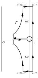
Figure 5. Contour $\Gamma$

The tail parts of $(c)$ are dominated by

$$\ll H^{-\frac{2\alpha}{k}}\int_{c+iT}^{c+i\infty}L(z)\zeta^{\beta^{2}}(z)H^{\frac{z}{k}}\frac{dz}{z}\ll H^{\frac{1-2\alpha}{k}+\frac{2\epsilon}{k}}T^{-2},$$

where we use the bound of $\widehat{w}$ from (5.5). Now consider the contour $\Gamma$ as in Figure 5 with $\sigma(T)=1-\frac{c_{0}}{\log T}$ for some constant $c_{0}>\frac{3}{2k}$. The contribution along the horizontal lines $[\sigma(T)\pm iT,c\pm iT]$ is

$$\ll H^{-\frac{2\alpha}{k}+\frac{2\epsilon}{k}}T^{-3}\int_{\sigma(T)}^{c}H^{\frac{\sigma}{k}}d\sigma\ll H^{\frac{1-2\alpha}{k}+\frac{2\epsilon}{k}}T^{-3}.$$

Further, the contribution along the arcs $\{\sigma(t)\pm it:\,0<t\leq T\}$ is

$$\ll H^{\frac{\sigma(T)}{k}-\frac{2\alpha}{k}+\frac{3\epsilon}{2k}}\int_{0}^{T}\frac{(\log t)^{|\beta|^{2}}}{1+|t|^{3}}dt\ll H^{\frac{\sigma(T)}{k}-\frac{2\alpha}{k}+\frac{3\epsilon}{2k}}.$$

Choosing $\epsilon=\frac{1}{\sqrt{\log H}}$ and $T=H^{\epsilon}$, the above estimates are bounded above by $O(H^{\frac{1-2\alpha}{k}}e^{-c_{1}\sqrt{\log H}})$ for some constant $c_{1}>0$. Using (5.8), Lemma 5.2 with the choice of $\epsilon=\frac{1}{\sqrt{\log H}}$ and following the proof of Theorem $5.2$ ([32]), we conclude that

$$I_{W}=\frac{2}{k^{\beta^{2}}}H^{\frac{1-2\alpha}{k}}(\log H)^{\beta^{2}-1}\bigg{\{}\sum_{0\leq j\leq N}\frac{k^{j}\lambda_{\alpha,j}(\beta^{2})}{\log^{j}H}+O_{\beta}\left(\frac{1}{\log^{N+1}H}\right)\bigg{\}}.$$

The class of functions $h\in\mathcal{G}_{\alpha}$ can be evaluated in a similar fashion as of the other family. ∎

Lemma 5.4.

Let $0\leq\alpha<1/2$ and $h\in\mathcal{M}_{\alpha}^{\mu}\cup\mathcal{G}_{\alpha}$. Recall $\mathcal{J}_{k,z}(H;h)$ from (3.1). Then

$$\mathcal{J}_{k,z}(H;h)=(1+O(H^{-\epsilon_{2}}))2H^{2}\sum_{d_{1}^{k},d_{2}^{k}\leq z}\frac{h(d_{1})h(d_{2})}{d_{1}^{k}d_{2}^{k}}\sum_{\lambda\geq 1}S\left(\frac{H\lambda}{(d_{1}^{k},d_{2}^{k})}\right)^{2}+O\left(\mathcal{E}_{k,h}(H)\right),$$

where

$$\mathcal{E}_{k,h}(H):=\sum_{d_{1}^{k},d_{2}^{k}\leq z}\sum_{0<|n_{1}|,|n_{2}|\leq N}\frac{|h(d_{1})h(d_{2})|}{n_{1}n_{2}}\small\mathbbm{1}_{0<\big{|}\frac{n_{1}}{d_{1}^{k}}-\frac{n_{2}}{d_{2}^{k}}\big{|}\leq\frac{BH^{\epsilon_{2}}}{X}}$$

for some constant $B>0$ and a small parameter $\epsilon_{2}>0$.

Proof.

Let $\sigma:\mathbb{R}\to\mathbb{R}$ be an integrable function such that $\widehat{\sigma}$ is supported in the interval $[-BH^{\epsilon_{2}},BH^{\epsilon_{2}}]$. We first show that

(5.9) $$\frac{1}{X}\int_{-\infty}^{\infty}\sigma\left(\frac{x}{X}\right)\Bigg{|}\sum_{\begin{subarray}{c}x<nd^{k}\leq x+H\\ d^{k}\leq z\end{subarray}}h(d)-H\sum_{d^{k}\leq z}\frac{h(d)}{d^{k}}\Bigg{|}^{2}dx$$

$$=2H^{2}\sum_{d_{1}^{k},d_{2}^{k}\leq z}\frac{h(d_{1})h(d_{2})}{d_{1}^{k}d_{2}^{k}}\sum_{\lambda\geq 1}S\left(\frac{H\lambda}{(d_{1}^{k},d_{2}^{k})}\right)^{2}+\mathcal{E}_{k,h}(H).$$

Observe that

$$\sum_{x/d^{k}<n\leq(x+H)/d^{k}}1=\frac{H}{d^{k}}+\psi\left(x/d^{k}\right)-\psi\left((x+H)/d^{k}\right),$$

where $\psi(y)=y-[y]-\frac{1}{2}$ with $[y]$ the integral part of $y$. We know the Fourier expansion of $\psi$ as

$$\psi(y)=-\frac{1}{2\pi i}\sum_{0<|n|\leq N}\frac{e(yn)}{n}+O\left(\min\bigg{\{}1,\frac{1}{N\|y\|}\bigg{\}}\right).$$

So, combining the above estimates we have

$$\sum_{\begin{subarray}{c}x<nd^{k}\leq x+H\\ d^{k}\leq z\end{subarray}}h(d)-H\sum_{d^{k}\leq z}\frac{h(d)}{d^{k}}=-\frac{1}{2\pi i}\sum_{d^{k}\leq z}h(d)\sum_{0<|n|\leq N}\frac{1}{n}e\left(\frac{nx}{d^{k}}\right)\left(1-e\left(\frac{nH}{d^{k}}\right)\right)$$

$$+O\bigg{(}\sum_{d^{k}\leq z}h(d)\left(\min\{1,1/(N\|x/d^{k}\|)\}+\min\{1,1/(N\|(x+H)/d^{k}\|)\}\right)\bigg{)}.$$

By choosing $N=X^{4}$, the above error term is $O(X^{-2})$ unless $\|x/d^{k}\|<X^{-2}$ or $\|(x+H)/d^{k}\|<X^{-2}$, which are not possible. This leads us to get an error term of size $O(X^{-1})$ to the main integral. Appealing to (5.9), we reduce it to study of the following expression with a negligible error:

(5.10) $$\frac{1}{4\pi^{2}}\sum_{\begin{subarray}{c}d_{1}^{k},d_{2}^{k}\leq z\\ 0<|n_{1}|,|n_{2}|\leq N\end{subarray}}\frac{h(d_{1})h(d_{2})}{n_{1}n_{2}}\left(1-e\left(\frac{n_{1}H}{d_{1}^{k}}\right)\right)\left(1-e\left(-\frac{n_{2}H}{d_{2}^{k}}\right)\right)\widehat{\sigma}\left(X\left(\frac{n_{2}}{d_{2}^{k}}-\frac{n_{1}}{d_{1}^{k}}\right)\right).$$

We shall consider separately those $(n_{1},n_{2},d_{1},d_{2})$ for which $n_{1}d_{2}^{k}-n_{2}d_{1}^{k}=0$ and those for which this does not hold.

If $n_{1}d_{2}^{k}-n_{2}d_{1}^{k}\neq 0$ then the above expression is essentially $\mathcal{E}_{k,h}(H)$. In the first case, we parameterizing $n_{1}$ and $n_{2}$ by $n_{1}=\frac{\lambda d_{1}^{k}}{(d_{1}^{k},d_{2}^{k})}$ and $n_{2}=\frac{\lambda d_{2}^{k}}{(d_{1}^{k},d_{2}^{k})}$ for $\lambda\in\mathbb{Z}\backslash\{0\}$. Therefore, using $|1-e(x)|=2|\sin(\pi x)|$, we obtain the main contribution in the expression (5.10) as

$$\frac{\widehat{\sigma}(0)}{\pi^{2}}\sum_{d_{1}^{k},d_{2}^{k}\leq z}\frac{h(d_{1})h(d_{2})}{d_{1}^{k}d_{2}^{k}}(d_{1},d_{2})^{2k}\sum_{\lambda\neq 0}\frac{1}{\lambda^{2}}\sin^{2}\left(\frac{\lambda\pi H}{(d_{1}^{k},d_{2}^{k})}\right).$$

It remains to connect $\mathcal{J}_{k,h}(H)$ and the integral (5.9). To do this we follow the argument given in [23, page 273] which also used in [7]: For an absolute constant $B$, we can find a smooth, integrable functions $\sigma_{-}$ and $\sigma_{+}$ such that their Fourier transforms $\widehat{\sigma}_{-}$ and $\widehat{\sigma}_{+}$ have the support $[-BH^{\epsilon_{2}},\,BH^{\epsilon_{2}}]$ and satisfied

$$\sigma_{-}\leq\mathbbm{1}_{[1,\,2]}\leq\sigma_{+}\,\mbox{ and }\,\Big{|}\int\Big{(}\sigma_{\pm}(x)-\mathbbm{1}_{[1,\,2]}(x)\Big{)}dx\Big{|}\ll H^{-\epsilon_{2}}.$$

Thus, we conclude that

$$\mathcal{J}_{k,h}(H)=(1+O(H^{-\epsilon_{2}}))\frac{1}{X}\int_{-\infty}^{\infty}\sigma_{\pm}\left(\frac{x}{X}\right)\bigg{|}\sum_{\begin{subarray}{c}x<nd^{k}\leq x+H\\ d^{k}\leq z\end{subarray}}h(d)-H\sum_{d^{k}\leq z}\frac{h(d)}{d^{k}}\bigg{|}^{2}dx.$$

∎

5.2. Density of rational points on binary forms

In this section, we collect essential lemmas regarding density of rational points on binary form which play an integral role to bound the non-diagonal terms occurred in Lemma 5.4. Let $F(x,y)$ be a binary form with integer coefficients, non-zero discriminant, and degree $d\geq 2$. For a positive number $Z$, let

$$\mathcal{N}_{F}(Z):=\{(x,y)\in\mathbb{R}^{2}:\,0<|F(x,y)|\leq Z\}$$

and

$$A_{F}=\mu\{(x,y)\in\mathbb{R}^{2}:\,|F(x,y)|\leq 1\},$$

where $\mu$ denotes the area of a set in $\mathbb{R}^{2}$. In 1933, Mahler [20] first obtain an asymptotic formula for the cardinality of $\mathcal{N}_{F}(Z)$, when $F$ is irreducible. Recently, Stewart and Xiao [31] have modified the result of Mahler and proved the following lemma.

Lemma 5.5.

Let $F$ be a binary form with integer coefficients, non-zero discriminant and degree $d\geq 3$. Then we have

$$|\mathcal{N}_{F}(Z)|=A_{F}Z^{\frac{2}{d}}+O_{F}\left(Z^{\theta}\right),$$

where $\theta=\frac{1}{d}$ if $F$ does not have a linear factor in $\mathbb{R}[x,y]$, and $\theta=\frac{1}{(d-1)}$ otherwise.

Following Heath-Brown’s proof of Theorem 8 in [12], they also proved the following.

Lemma 5.6.

Let $F$ be a binary form with integer coefficients, non-zero discriminant and degree $d\geq 3$. Let $Z$ be a positive real number and $\gamma$ be a real number larger than $\frac{1}{d}$. The number of pairs of integers $(x,y)$ with

$$0<|F(x,y)|\leq Z$$

for which

$$\max\{|x|,|y|\}>Z^{\gamma}$$

is

$$O_{F}\left(Z^{\frac{1}{d}}\log Z+Z^{1-(d-2)\gamma}\right).$$

As an application of the above lemmas, we bound the term $\mathcal{E}_{k,h}(H)$ as follows.

Lemma 5.7.

Let $\epsilon>0$ be given, $\epsilon_{\alpha,k}>0$ depends on $\epsilon,\alpha$ and $k$. Suppose that $1<\nu\leq 2$. Recall $\mathcal{E}_{k,h}(H)$ from Lemma 5.4. For $0\leq\alpha<\frac{1}{2}$ we have

$$\mathcal{E}_{k,h}(H)\ll\begin{cases}H^{\frac{1-2\alpha}{2}-\frac{\epsilon}{5}}&\mbox{ if }z\leq\min\big{\{}X^{\frac{1}{(1-\alpha)}}H^{-\frac{1+2\alpha}{2-2\alpha}-\epsilon},H^{\frac{1-2\alpha}{2-2\alpha}-\epsilon}X^{\frac{1}{2-2\alpha}}\big{\}},\,H\leq X^{\frac{2+\alpha}{3+2\alpha}-\epsilon},\,k=2,\\ H^{\frac{1-2\alpha}{k}-\frac{\epsilon}{k}}&\mbox{ if }z\leq\min\big{\{}X^{\frac{2}{\nu(2-\alpha)}}H^{\frac{1-2\alpha}{\nu(2-\alpha)}-\epsilon},X^{\frac{\nu}{2(\nu-\alpha)}}H^{\frac{1-2\alpha}{2(\nu-\alpha)}-\epsilon},X^{\frac{2(k-\nu)}{(4-\nu)k-2\nu}-\epsilon}\big{\}},\,k\geq 3.\end{cases}$$

For $\frac{1}{2}<\alpha<1$, we obtain $\mathcal{E}_{k,h}(H)\ll H^{-\epsilon_{\alpha,k}}$, whenever

$$z\leq\begin{cases}X^{\frac{1}{2(1-\alpha)}}H^{-\frac{1}{2(1-\alpha)}-\epsilon}&\mbox{ if }k=1,\\ \min\big{\{}X^{\frac{1}{1-\alpha}}H^{-\frac{1}{1-\alpha}-\epsilon},X^{\frac{1}{2-2\alpha}}H^{-\epsilon}\big{\}}&\mbox{ if }H\leq X^{\frac{2+\alpha}{4}-\epsilon}\text{ and }k=2,\\ \min\big{\{}X^{\frac{2}{\nu(2-\alpha)}-\epsilon},X^{\frac{\nu}{2(\nu-\alpha)}-\epsilon},X^{\frac{2(k-\nu)}{(4-\nu)k-2\nu}-\epsilon}\big{\}}&\mbox{ if }k\geq 3.\end{cases}$$

Suppose that $1\leq\alpha<2$ and $z\leq 2X$. In this case, we have $\mathcal{E}_{k,h}(H)\ll H^{-\epsilon_{\alpha,k}}$, provided that $H\leq X^{1-\epsilon}$ if $k\in\mathbb{N}\setminus\{2\}$ and $H\leq X^{\frac{2+\alpha}{4}-\epsilon}$ if $k=2$.

Proof.

We shall prove case by case with respect to different values of $k$.
Case 1. Assume that $k=1$. Splitting $n_{j}$ and $d_{j}$ dyadically, for any $D_{1},D_{2}\leq z$ and any $N_{1},N_{2}\leq N$, we have

$$\mathcal{E}_{1,h}(H) \ll z^{2\epsilon_{1}}\frac{(\log X)^{4}}{(D_{1}D_{2})^{\alpha}}\min\bigg{\{}\frac{1}{N_{1}},\frac{H}{D_{1}}\bigg{\}}\min\bigg{\{}\frac{1}{N_{2}},\frac{H}{D_{2}}\bigg{\}}$$

$$\times\sum_{\begin{subarray}{c}n_{1}\sim N_{1}\\ n_{2}\sim N_{2}\end{subarray}}\#\Big{\{}d_{j}\sim D_{j}:\,0<\bigg{|}\frac{n_{1}}{d_{1}}-\frac{n_{2}}{d_{2}}\bigg{|}\leq\frac{BH^{\epsilon_{2}}}{X}\Big{\}}.$$

Note that the solution of the above system exist only if $N_{1}D_{2}\asymp N_{2}D_{1}$. In this case, the innermost sum is equivalent to

$$\#\Big{\{}r_{1}\sim N_{2}D_{1};r_{2}\sim N_{1}D_{2}:\,0<|r_{1}-r_{2}|\leq Y\Big{\}},$$

where $Y=\frac{BH^{\epsilon_{2}}D_{1}D_{2}}{X}$. Observe that

$$\#\Big{\{}r_{1}\sim N_{2}D_{1};r_{2}\sim N_{1}D_{2}:\,0<|r_{1}-r_{2}|\leq Y\Big{\}}\ll\max\{N_{2}D_{1}Y,\,N_{1}D_{2}Y,\,Y^{2}\}.$$

We see that the bound of $\mathcal{E}_{1,h}(H)$ attains its maximum only when $N_{j}=\frac{H}{D_{j}}$ for $j=1,2$. Therefore

$$\mathcal{E}_{1,h}(H) \ll z^{2\epsilon_{1}}H^{\epsilon_{2}}\frac{(D_{1}D_{2})^{1-\alpha}H}{X}(\log X)^{4}\ll z^{2\epsilon_{1}}H^{\epsilon_{2}}\frac{z^{2(1-\alpha)}H}{X}(\log X)^{4}$$

$$\ll\begin{cases}H^{-\epsilon_{\alpha,1}}&\mbox{ if }z\leq X^{\frac{1}{2(1-\alpha)}}H^{-\frac{1}{2(1-\alpha)}-\epsilon},\,\frac{1}{2}<\alpha<1,\\ H^{-\epsilon_{\alpha,1}}&\mbox{ if }z\leq 2X,H\leq X^{1-\epsilon},\,1\leq\alpha<2,\end{cases}$$

by taking $\epsilon_{1}$ and $\epsilon_{2}$ suitably small.

Case 2. Assume that $k=2$ and $0\leq\alpha<\frac{1}{2}$. We choose $\epsilon_{2}=\frac{\epsilon}{4}$ and $\epsilon_{1}\ll\epsilon^{2}$. Using $h(d)\ll\frac{1}{d^{\alpha-\epsilon_{1}}}$, we can directly follow the way in proof of Proposition $5$ [7, Eq. (32)] to get that $\mathcal{E}_{2,h}(H)\ll H^{\frac{1-2\alpha}{2}-\frac{\epsilon}{5}}$ only when $z\leq\min\Big{\{}X^{\frac{1}{1-\alpha}}H^{-\frac{1+2\alpha}{2-2\alpha}-\epsilon},X^{\frac{1}{2-2\alpha}}H^{\frac{1-2\alpha}{2-2\alpha}-\epsilon}\Big{\}}$ and $H\leq X^{\frac{2+\alpha}{3+2\alpha}-\epsilon}$.

Now assume that $\frac{1}{2}<\alpha<1$. Again we go along with the proof of Proposition $5$ of [7, Eq. (32)]. If $\sqrt{\frac{n_{2}}{n_{1}}}$ is quadratic irrational then $\mathcal{E}_{2,h}(H)$ is bounded above by

(5.11) $$\ll z^{\epsilon_{1}}\frac{H^{\epsilon_{2}}}{D_{1}^{\alpha}D_{2}^{\alpha}}\left(\frac{D_{1}D_{2}H}{X}+1+\frac{D_{1}D_{2}}{X^{1/2}}\right)\ll H^{-\epsilon_{\alpha,k}},$$

whenever $z\leq\min\Big{\{}X^{\frac{1}{1-\alpha}}H^{-\frac{1}{1-\alpha}-\epsilon},X^{\frac{1}{2-2\alpha}}H^{-\epsilon}\Big{\}}$. The important observation is that

$$\#\Big{\{}(d_{1}\sim D_{1};d_{2}\sim D_{2}:\,0<|n_{1}d_{2}^{2}-n_{2}d_{1}^{2}|\leq\frac{BH^{\epsilon_{2}}D_{1}^{2}D_{2}^{2}}{X}\Big{\}}\neq 0,$$

only if $D_{1}D_{2}\gg X^{1/2}H^{-\epsilon_{2}/2}$. If $\sqrt{\frac{n_{2}}{n_{1}}}$ is rational then $\mathcal{E}_{2,h}(H)$ is bounded above by

(5.12) $$\ll z^{\epsilon_{1}}\frac{H^{2}}{(D_{1}D_{2})^{\alpha}X}\ll H^{-\epsilon_{\alpha,2}},$$

since $H\leq X^{\frac{2+\alpha}{4}-\epsilon}$ and $D_{1}D_{2}\gg X^{1/2}H^{-\epsilon_{2}/2}$.

Suppose that $1\leq\alpha<2$. From (5.11) and (5.12), we estimate that $\mathcal{E}_{2,h}(H)\ll H^{-\epsilon_{\alpha,2}}$, since $H\leq X^{\frac{2+\alpha}{4}-\epsilon}$.

Case 3. Let $k\geq 3$. First assume that $1\leq\alpha<2$. Since $z\leq 2X$, using Lemma 5.5,

$$\mathcal{E}_{k,h}(H)\ll z^{2\epsilon_{1}/k}(\log X)^{4}(D_{1}D_{2})^{-\alpha}\left(\frac{H^{\epsilon_{2}}D_{1}^{k}D_{2}^{k}}{X}\right)^{\frac{2}{k}}\ll H^{-\epsilon_{\alpha,k}},$$

Now, we consider $\alpha\in[0,1)\setminus\{1/2\}$. Let us define

$$\mathcal{R}:=\#\Big{\{}d_{1}\sim D_{1},d_{2}\sim D_{2}:\,0<|n_{1}d_{2}^{k}-n_{2}d_{1}^{k}|\leq\frac{BH^{\epsilon_{2}}D_{1}^{k}D_{2}^{k}}{X}\Big{\}}$$

For $1<\nu\leq 2$ we divide $\mathcal{R}$ into two parts as follows

$$\mathcal{R}_{\nu}(n_{1},n_{2}):=\#\Big{\{}d_{j}\sim D_{j}:\,D_{j}\leq z^{1/k},\,D_{1}D_{2}<z^{\nu/k},\,0<|n_{1}d_{2}^{k}-n_{2}d_{1}^{k}|\leq\frac{BH^{\epsilon_{2}}D_{1}^{k}D_{2}^{k}}{X}\Big{\}}$$

and

$$\mathcal{R}_{v}^{C}(n_{1},n_{2}):=\#\Big{\{}d_{j}\sim D_{j}:\,D_{j}\leq z^{1/k},\,D_{1}D_{2}\geq z^{\nu/k},\,0<|n_{1}d_{2}^{k}-n_{2}d_{1}^{k}|\leq\frac{BH^{\epsilon_{2}}D_{1}^{k}D_{2}^{k}}{X}\Big{\}}.$$

Therefore,

$$\mathcal{E}_{k,h}(H)\ll z^{2\epsilon_{1}/k}\frac{(\log X)^{2}}{(D_{1}D_{2})^{\alpha}}\sum_{n_{j}\leq N}\frac{1}{n_{1}n_{2}}\left(\mathcal{R}_{\nu}(n_{1},n_{2})+\mathcal{R}_{\nu}^{C}(n_{1},n_{2})\right).$$

We bound the above quantities with the help of lemmas which are presented in the beginning of this sub-section. Lemma 5.5 gives us

$$\mathcal{R}_{\nu}(n_{1},n_{2})\ll\left(\frac{H^{\epsilon_{2}}D_{1}^{k}D_{2}^{k}}{X}\right)^{\frac{2}{k}}.$$

Let us put $Z=\frac{BH^{\epsilon_{2}}D_{1}^{k}D_{2}^{k}}{X}$. The range of $d_{1}$ and $d_{2}$ imply that if $D_{1}D_{2}>z^{\nu/k}$ then $\max\{D_{1},D_{2}\}>z^{\nu/2k}$. In the view of Lemma 5.6 with $\gamma=\frac{1}{k}+\frac{2-\nu}{k(k-2)}$,

$$\mathcal{R}_{\nu}^{C}(n_{1},n_{2}) \ll\#\Big{\{}(d_{1},d_{2})\in\mathbb{Z}^{2}:\,\max\{D_{1},D_{2}\}>Z^{\gamma},\,0<|n_{1}d_{2}^{k}-n_{2}d_{1}^{k}|\leq Z\Big{\}}$$

$$\ll(Z^{1/k}\log Z+Z^{1-(k-2)\gamma})\ll Z^{\frac{\nu}{k}},$$

provided that $Z^{\gamma}\leq z^{\frac{\nu}{2k}}$. The condition $Z^{\gamma}\leq z^{\frac{\nu}{2k}}$ is equivalent to $z\leq(XH^{-\epsilon_{2}})^{\frac{2(k-\nu)}{(4-\nu)k-2\nu}}$.
Combining these estimates, we find that for $z\leq(XH^{-\epsilon_{2}})^{\frac{2(k-\nu)}{(4-\nu)k-2\nu}},$

$$\mathcal{E}_{k,h}(H)\ll z^{2\epsilon_{1}/k}\frac{(\log X)^{4}}{(D_{1}D_{2})^{\alpha}}\left(\left(\frac{H^{\epsilon_{2}}D_{1}^{k}D_{2}^{k}}{X}\right)^{\frac{2}{k}}+Z^{\frac{\nu}{k}}\right).$$

Subcase 3.1. Assume that $0\leq\alpha<\frac{1}{2}$. With the choice of $\epsilon_{2}=\frac{\epsilon}{k}$ and $\epsilon_{1}\ll\epsilon^{2}$, we have

$$\mathcal{E}_{k,h}(H)\ll H^{\frac{1-2\alpha}{k}-\frac{\epsilon}{k}},$$

provided that $z\leq\min\Big{\{}X^{\frac{2}{\nu(2-\alpha)}}H^{\frac{1-2\alpha}{\nu(2-\alpha)}-\epsilon},X^{\frac{\nu}{2(\nu-\alpha)}}H^{\frac{1-2\alpha}{2(\nu-\alpha)}-\epsilon},X^{\frac{2(k-\nu)}{(4-\nu)k-2\nu}-\epsilon}\Big{\}}$ and $\nu>1.4$.

Subcase 3.2. Assume that $\frac{1}{2}<\alpha<1$. In this case,

$$\mathcal{E}_{k,h}(H)\ll H^{-\epsilon_{\alpha,k}}$$

only when $z\leq\min\Big{\{}X^{\frac{2}{\nu(2-\alpha)}-\epsilon},X^{\frac{\nu}{2(\nu-\alpha)}-\epsilon},X^{\frac{2(k-\nu)}{(4-\nu)k-2\nu}-\epsilon}\Big{\}}$. This completes the proof. ∎

Proof of Proposition 3.1.

Combining Lemma 5.2, Lemma 5.4 and Lemma 5.7 finishes the proof. ∎

Proof of Proposition 3.2.

For $f\in\mathcal{F}_{\alpha,\beta,k}$ with $\alpha>\frac{1}{2}$, recall $I_{W}$ from 5.3 and define

$$I_{S}=2H^{2}\sum_{d_{1},d_{1}\geq 1}\frac{h(d_{1})h(d_{2})}{d_{1}^{k}d_{2}^{k}}\sum_{\lambda\geq 1}S\left(\frac{H\lambda}{(d_{1}^{k},d_{2}^{k})}\right)^{2}.$$

Following the proof of Lemma 5.2 we are only left to show that $I_{S}-I_{W}$ is of size $O(H^{-\epsilon_{\alpha,k}})$. In view of (5.7), we have

$$|I_{S}-I_{W}| \ll\sum_{d_{1},d_{2}\geq 1}\frac{h(d_{1})h(d_{2})}{d_{1}^{k}d_{2}^{k}}\sum_{\lambda\geq 1}\frac{(d_{1},d_{2})^{2k}}{\lambda^{2}}\mathds{1}\left(\frac{H\lambda}{(d_{1}^{k},d_{2}^{k})}\geq H^{\epsilon^{\prime}}\right)\ll H^{\frac{(1-\epsilon^{\prime})(1-2\alpha+2\epsilon_{1})}{k}}\ll H^{-\epsilon_{\alpha,k}},$$

for suitably small choice of $\epsilon^{\prime}$ and $\epsilon_{1}$. Since $2\sin^{2}{x}=1-\cos{2x}$, by using Lemma 5.1,

$$I_{S,z}=\sum_{d_{1},d_{2}\geq 1}\frac{h(d_{1})h(d_{2})}{d_{1}^{k}d_{2}^{k}}(d_{1},d_{2})^{2k}\left(\left\{\ \frac{H}{(d_{1},d_{2})^{k}}\right\}-\left\{\ \frac{H}{(d_{1},d_{2})^{k}}\right\}^{2}\right)+O\left(H^{-\epsilon_{\alpha,k}}\right).$$

Denoting $d:=(d_{1},d_{2})$ and writing $d_{1}=e_{1}d$, $d_{2}=e_{2}d$, we have $(e_{1},e_{2})=1$. By this change of variables, the main term of above expression can be simplified and reduce to $c_{h,k}(H)$, which is the main term of this proposition (see (2.12)). Hence, appealing to Lemma 5.4 and Lemma 5.7 completes the proof. ∎

6. Proof of Proposition 3.3

We collect some standard lemmas from [7] which are main tools to prove the proposition.

Lemma 6.1.

Let $N,T\geq 1$ and $V>0$. Let $A(s)=\sum_{n\leq N}a_{n}n^{-s}$ be a Dirichlet polynomial and let $S=\sum_{n\leq N}|a_{n}|^{2}$. Let $\mathcal{T}$ be a set of $1$-spaced points $t_{r}\in[-T,T]$ such that $A(it_{r})\geq V$. Then

$$|\mathcal{T}|\ll\left(SNV^{-2}+T\min\{SV^{-2},S^{3}NV^{-6}\}\right)(\log 2NT)^{6}.$$

Lemma 6.2.

Let $A(s)$ be as in Lemma 6.1. Then

$$\int_{-T}^{T}|A(it)|^{2}dt=(T+O(N))\sum_{n\leq N}|a_{n}|^{2}.$$

Lemma 6.3.

If $F:\mathbb{R}\to\mathbb{C}$ is a square-integrable function and $H\leq X$, then

$$\int_{X}^{2X}|F(x+H)-F(x)|^{2}dx\ll\sup_{\theta\in\big{[}\frac{H}{3X},\frac{3H}{X}\big{]}}\int_{X}^{3X}|F(u+\theta u)-F(u)|^{2}du.$$

Proof of Proposition 3.3.

To estimate $\mathcal{K}_{k,z}(H;h)$ we split the interval $[z^{1/k},(2X)^{1/k}]$ into dyadic intervals according to the size of $d$. Thus it suffices to bound

(6.1) $$\frac{1}{X}\int_{X}^{2X}\bigg{|}\sum_{\begin{subarray}{c}x<nd^{k}\leq x+H\\ d\sim D\end{subarray}}h(d)-H\sum_{d\thicksim D}\frac{h(d)}{d^{k}}\bigg{|}^{2}dx$$

for each $D\in[z^{1/k},(2X)^{1/k}]$ such that $(\alpha,k)\neq(0,1)$. Let’s look at

$$A(x):=\sum_{\begin{subarray}{c}nd^{k}\leq x\\ d\sim D\end{subarray}}h(d)-xB_{h}(k)\quad\mbox{and}\quad B_{h}(s):=\sum_{d\sim D}\frac{h(d)}{d^{s}}.$$

Using Perron’s summation formula, we deduce that

$$A(e^{y})=\frac{1}{2\pi i}\int_{2-i\infty}^{2+i\infty}\frac{e^{ys}}{s}\zeta(s)B_{h}(ks)ds-e^{y}B_{h}(k).$$

By moving the contour of integration to the line $\Re(s)=\frac{1}{2}$ we capture the pole at $s=1$ and the residue at this point cancels with the second term $e^{y}B_{h}(k)$. Thus, for any real $\omega$ we obtain that

$$\frac{A(e^{w+x})-A(e^{x})}{e^{x/2}}=\frac{1}{2\pi}\int_{-\infty}^{\infty}\frac{e^{w(1/2+it)}-1}{1/2+it}e^{itx}\zeta(1/2+it)B_{h}(k/2+kit)dt.$$

The Plancherel formula gives

$$\int_{0}^{\infty}|A(e^{u+w})-A(e^{u})|^{2}\frac{du}{e^{u}}\ll\int_{\mathbb{R}}\bigg{|}\frac{e^{w(1/2+it)}-1}{1/2+it}\bigg{|}^{2}|\zeta(1/2+it)B_{h}(k/2+kit)|^{2}dt.$$

Imposing Lemma 6.3,

$$\frac{1}{X}\int_{X}^{2X}|A(x+H)-A(x)|^{2}dx\ll\frac{1}{X}\int_{X}^{2X}|A(u(1+\theta))-A(u)|^{2}du$$

for some $\theta\in\big{[}\frac{H}{3X},\frac{3H}{X}\big{]}$. Now we take $w$ satisfying $e^{w}=1+\theta$, so that $w\asymp\frac{H}{X}$. Therefore,

(6.2) $$\frac{1}{X}\int_{X}^{2X}|A(x+H)-A(x)|^{2}dx \ll X\int_{0}^{\infty}|A(u(1+\theta))-A(u)|^{2}\frac{du}{u^{2}}$$

$$\ll X\int_{\mathbb{R}}\bigg{|}\frac{e^{w(1/2+it)}-1}{1/2+it}\bigg{|}^{2}|\zeta(1/2+it)B_{h}(k/2+kit)|^{2}dt.$$

The well-known sub-convexity bound tells that $|\zeta(1/2+it)|\ll|t|^{1/6}(\log|t|)^{2}$ for $|t|\geq 2$ and $B_{h}(k/2+kit)\ll D^{1-\alpha-\frac{k}{2}+\epsilon_{1}}$. Therefore, the integral in the right hand side of (6.2) with $|t|\geq X^{2}$ contributes

$$\ll XD^{1-\alpha-\frac{k}{2}}\int_{X^{2}}^{\infty}|t|^{-5/3+\epsilon}dt\ll X^{-\frac{1}{3}+2\epsilon}D^{1-\alpha-\frac{k}{2}}\ll X^{-\frac{1}{4}}.$$

Splitting into the regions $|t|\leq\frac{X}{H}$ and $2^{l}<|t|\leq 2^{l+1}$ with $\frac{X}{2H}\leq 2^{l}\leq X^{2}$, the right hand side of (6.2) is bounded by

(6.3) $$\ll H\bigg{(}\sup_{X/H\leq T\leq X^{2}}\frac{1}{T}\int_{|t|\leq T}|\zeta(1/2+it)B_{h}(k/2+kit)|^{2}dt\bigg{)}+O(X^{-\frac{1}{4}}).$$

Case 1: Assume that the Lindelöf hypothesis is true. Let $0\leq\alpha<\frac{1}{2}$ and $\delta>0$ be sufficiently small. By using Lemma 6.2 we get that (6.3) is bounded above by

$$\ll\Big{(}\frac{H}{D^{k+2\alpha-1}}+\frac{H}{TD^{k+2\alpha-2}}\Big{)}T^{\delta}D^{2\epsilon_{1}}.$$

Since $\delta$ and $\epsilon_{1}$ are sufficiently small, $T^{\delta}D^{2\epsilon_{1}}\ll H^{\epsilon/2k}$. Thus, under the ranges $X/H\leq T\leq X^{2}$, $D\in[z^{1/k},(2X)^{1/k}]$ and $z\geq H^{1+\epsilon}$ with the hypothesis $H\leq X^{\frac{k}{k+1}-\epsilon}$, the expression in (6.3) is dominated by

$$\Big{(}\frac{H}{D^{k+2\alpha-1}}+\frac{H^{2}}{XD^{k+2\alpha-2}}\Big{)}H^{\frac{\epsilon}{2k}}\ll\Big{(}H^{\frac{1-2\alpha}{k}-\epsilon\frac{2k+4\alpha-3}{2k}}+H^{\frac{1-2\alpha}{k}-\epsilon\frac{4k^{2}+4k\alpha-k+2}{2k^{2}}}\Big{)}\ll H^{\frac{1-2\alpha}{k}-\epsilon\frac{2k+4\alpha-3}{2k}}.$$

Now we consider $\frac{1}{2}<\alpha<1$. Similar to above estimates, (6.3) $\ll H^{-\epsilon/2}$, since $z\geq H^{1+\epsilon}$ and $H\leq X^{\frac{k}{k-2\alpha+2}-\epsilon}$.

Case 2. Now we will see what happens unconditionally.

Subcase 1. Assume that $k\geq 2$ and $0\leq\alpha<\frac{1}{2}$. Consider the following set

$$S(V)=\{t\in[-T,T]:\,|B_{h}(k/2+kit)|\leq f(D)\},$$

where $f(D)$ is a function of $D$ will be chosen later. From the Cauchy-Schwarz inequality and fourth moment of Riemann $\zeta$-function, $S(V)$ contributes to (6.3) as

$$\ll\frac{H}{T}\bigg{(}\int_{|t|\leq T}|\zeta(1/2+it)|^{4}\bigg{)}^{1/2}\bigg{(}\int_{S(V)}|B_{h}(k/2+kit)|^{4}\bigg{)}^{1/2}\ll H{(\log{T})}^{2}f(D)^{2}\ll H^{\frac{1-2\alpha}{k}-\epsilon}$$

provided that $f(D)\ll H^{\frac{1-2\alpha-k}{2k}-\epsilon}$. Since $D\geq z^{1/k}\geq H^{1/k+\epsilon/k}$, we can choose $f(D)=D^{\frac{1-2\alpha-k}{2}-\epsilon}$.

Note that $|B_{h}(k/2+ikt)|\leq(2D)^{1-\alpha-\frac{k}{2}+\epsilon_{1}}$. Let’s examine the set

$$S(V)^{C}=\{t\in[-T,T]:\,V\leq|B_{h}(k/2+kit)|<2V\}.$$

Splitting dyadically, it is enough to show that for each $V\in[f(D),(2D)^{1-\alpha-\frac{k}{2}+\epsilon_{1}}]$ and $T\in[X/H,X^{2}]$,

$$\frac{H}{T}V^{2}\int_{S(V)^{C}}|\zeta(1/2+it)|^{2}dt\ll H^{\frac{1-2\alpha}{k}-\epsilon}.$$

Further, a trivial estimate shows that

$$\sum_{d\sim D}\frac{h^{2}(d)}{d^{k}}\ll\frac{1}{D^{k+2\alpha-1-2\epsilon_{1}}}.$$

Thus Lemma 6.1 gives

$$|S(V)^{C}|\ll\left(\frac{1}{D^{k+2\alpha-2}}V^{-2}+T\min\Big{\{}\frac{1}{D^{k+2\alpha-1}}V^{-2},\frac{1}{D^{3k+6\alpha-4}}V^{-6}\Big{\}}\right)D^{8\epsilon_{1}}.$$

We start with bounding the first term of $|S(V)^{C}|$. Using the best known sub-convexity bound for the $\zeta$-function due to J. Bourgain [4], in the range of $T\in[X/H,X^{2}]$ and $D\in[z^{1/k},(2X)^{1/k}]$, we obtain

$$\frac{H}{T}V^{2}\int_{S(V)^{C}}|\zeta(1/2+it)|^{2}dt\ll\frac{HD^{8\epsilon_{1}}}{T^{29/42-\epsilon}D^{k+2\alpha-2}}\ll H^{\frac{1-2\alpha}{k}-\frac{\epsilon}{2}}$$

since $H\leq X^{\frac{29k}{29k+42}-\epsilon}$ and $\epsilon_{1}$ is sufficiently small.

Now we inspect the second term in the above bound of $|S(V)^{C}|$. Applying Cauchy-Schwarz inequality and the fourth moment of Riemann $\zeta$-function, we deduce that

$$\frac{H}{T}V^{2}\int_{S(V)^{C}}|\zeta(1/2+it)|^{2}dt \ll\frac{H}{T}V^{2}|S(V)^{C}|^{1/2}\bigg{(}\int_{|t|\leq T}|\zeta(1/2+it)|^{4}dt\bigg{)}^{1/2}$$

$$\ll HV^{2}\min\Big{\{}\frac{V^{-2}}{D^{k+2\alpha-1}},\frac{V^{-6}}{D^{3k+6\alpha-4}}\Big{\}}^{1/2}D^{4\epsilon_{1}}$$

$$\ll H\frac{V^{1/2}}{D^{(k+2\alpha-1)/4}}\frac{V^{-1/2}}{D^{(3k+6\alpha-4)/4}}D^{4\epsilon_{1}}\ll H^{\frac{1-2\alpha}{k}-\epsilon/2}$$

provided that $z>H^{\frac{k+2\alpha-1}{k+2\alpha-5/4}+\epsilon}$. Note that $\mathcal{K}_{k,z}(H;h)$ is bounded above $\log{H}$ times the dyadic expression in (6.1) and hence $\mathcal{K}_{k,z}(H;h)\ll H^{\frac{1-2\alpha}{k}-\frac{\epsilon}{3}}$.

Subcase 2. Assume that $k\geq 1$ and $\frac{1}{2}<\alpha<1$. Similar to Subcase 1, the result follows. ∎

7. Proof of Proposition 3.4 and Proposition 3.5

In this section, we prove the main propositions related to discrete variance for our family of multiplicative functions.

Preparation of proofs

Expanding square to $\operatorname{Var}_{\mathcal{D}}(\mathcal{F}_{\alpha,\beta,k})$ and using (1.1), we obtain

(7.1) $$\operatorname{Var}_{\mathcal{D}}(\mathcal{F}_{\alpha,\beta,k})=S_{1}-\widetilde{c}_{h,k}^{2}H^{2}+O\left(\frac{H^{2}}{X}X^{\max\big{\{}\frac{1-\alpha}{k}+\epsilon_{1},\,0\big{\}}}\right),$$

where

$$S_{1}:=\frac{1}{X}\sum_{j_{1},j_{2}=1}^{H}\sum_{n\leq X}f(n+j_{1})f(n+j_{2}).$$

Let us denote

$$f_{z}(n):=\sum_{\begin{subarray}{c}d^{k}\mid n\\ d\leq z\end{subarray}}h(d)\quad\text{ and }\quad f_{z}^{c}(n):=\sum_{\begin{subarray}{c}d^{k}\mid n\\ d>z\end{subarray}}h(d)$$

so that $f(n)=f_{z}(n)+f_{z}^{c}(n)$, where $z$ to be chosen later. Using Cauchy- Schwarz inequality, we have

$$\bigg{|}\sum_{n\leq X}f(n+j_{1})f(n+j_{2})-f_{z}(n+j_{1})f_{z}(n+j_{2})\bigg{|}\ll\bigg{(}\sum_{n\leq X}|f_{z}^{c}(n+j_{1})|^{2}\bigg{)}^{\frac{1}{2}}\bigg{(}\sum_{n\leq X}|f_{z}(n+j_{2})|^{2}\bigg{)}^{\frac{1}{2}}.$$

Applying the Chinese remainder theorem and $h(d)\ll\frac{1}{d^{\alpha-\epsilon_{1}}}$, we obtain

$$\sum_{n\leq X}|f_{z}^{c}(n+j_{1})|^{2}=\sum_{n\leq X}\bigg{(}\sum_{\begin{subarray}{c}d^{k}\mid n+j_{1}\\ d>z\end{subarray}}h(d)\bigg{)}^{2}\ll\frac{X+j_{1}}{z^{2(k+\alpha-\epsilon_{1}-1)}}.$$

It is easy to make out

$$\sum_{n\leq X}|f_{z}(n+j_{2})|^{2}\ll X.$$

Combining altogether we deduce that

$$S_{1}=\frac{1}{X}\sum_{j_{1},j_{2}=1}^{H}\sum_{n\leq X}f_{z}(n+j_{1})f_{z}(n+j_{2})+O\left(H^{2}z^{-(k+\alpha-\epsilon_{1}-1)}\right).$$

Again using the Chinese remainder theorem we get

$$\sum_{n\leq X}f_{z}(n+j_{1})f_{z}(n+j_{2}) =X\sum_{d_{1},d_{2}\geq 1}\frac{h(d_{1})h(d_{2})}{[d_{1},d_{2}]^{k}}\varrho(j_{1},j_{2},d_{1},d_{2})$$

$$+O(z^{2(1-\alpha+\epsilon_{1})})+O\bigg{(}X\sum_{d_{1}>z;d_{2}\geq 1}\frac{|h(d_{1})h(d_{2})|}{d_{1}^{k}d_{2}^{k}}\bigg{)},$$

where $\varrho(j_{1},j_{2},d_{1},d_{2})$ is the number of solution of the congruence system $n\equiv-j_{1}\left(\mathrm{mod}\,d_{1}^{k}\right)$ and $n\equiv-j_{2}\left(\mathrm{mod}\,d_{2}^{k}\right)$. The error term of the above estimate is bounded above by

$$\ll z^{2(1-\alpha+\epsilon_{1})}+Xz^{-(k+\alpha-\epsilon_{1}-1)}.$$

By setting $z=X^{\frac{1}{k-\alpha+1+\epsilon_{1}}},$

(7.2) $$S_{1}=\sum_{j_{1},j_{2}=1}^{H}A(j_{1},j_{2})+O\left(H^{2}X^{-\frac{k+\alpha-1-\epsilon_{1}}{k-\alpha+1+\epsilon_{1}}}\right),$$

where

$$A(j_{1},j_{2}):=\sum_{d_{1},d_{2}\geq 1}\frac{h(d_{1})h(d_{2})}{[d_{1},d_{2}]^{k}}\varrho(j_{1},j_{2},d_{1},d_{2}).$$

To state our next lemma we use the following notations.

$$Q_{h}(s)=\begin{cases}\prod_{p}\left(1+\frac{p^{k}h(p)^{2}}{p^{s}(p^{k}+2h(p))}\right)&\mbox{ if }h\in\mathcal{M}_{\alpha}^{\mu},\\ \prod_{p}\left(1-\frac{h(p)^{2}}{p^{s}}\right)^{-1}&\mbox{ if }h\in\mathcal{G}_{\alpha},\end{cases}\quad\text{ and }\quad e_{h}=\begin{cases}\prod_{p}\left(1+\frac{2h(p)}{p^{k}}\right)&\mbox{ if }h\in\mathcal{M}_{\alpha}^{\mu},\\ \prod_{p}\frac{p^{k}+h(p)}{p^{k}-h(p)}&\mbox{ if }h\in\mathcal{G}_{\alpha}.\end{cases}$$

Lemma 7.1.

Let $-\frac{1}{2}<\gamma<0$ and $0\leq\alpha<2$. We have

$$R(H):=\sum_{j_{1}=1}^{H}\sum_{j_{2}=1}^{H}A(j_{1},\,j_{2})=\widetilde{c}_{h,k}^{2}H^{2}+2e_{h}I_{h,\alpha,\gamma}(H),$$

where

(7.3) $$I_{h,\alpha,\gamma}(H):=\frac{1}{2\pi i}\int_{(\gamma)}H^{s+1}\chi(s)\zeta(1-s)Q_{h}(k+ks)\frac{ds}{s(s+1)}.$$

Proof.

Notice that

$$A(j_{1},j_{2}) =\sum_{\begin{subarray}{c}d_{1},d_{2}\geq 1\\ (d_{1},d_{2})^{k}\mid\,|j_{1}-j_{2}|\end{subarray}}\frac{h(d_{1})h(d_{2})}{[d_{1},d_{2}]^{k}}=\begin{cases}e_{h}\displaystyle\sum_{d^{k}\mid\,|j_{1}-j_{2}|}\frac{h(d)^{2}}{d^{k}}\prod_{p|d}\left(1+\frac{2h(p)}{p^{k}}\right)^{-1}&\mbox{ if }\,h\in\mathcal{M}_{\alpha}^{\mu},\\ e_{h}\displaystyle\prod_{p^{k}\mid\,|j_{1}-j_{2}|}\left(1-\frac{h(p)^{2}}{p^{k}}\right)^{-1}&\mbox{ if }\,h\in\mathcal{G}_{\alpha}.\end{cases}$$

This implies

$$R(H)=e_{h}\sum_{j_{1}=1}^{H}\sum_{j_{2}=1}^{H}f_{h}(|j_{1}-j_{2}|),$$

where

$$f_{h}(r)=\begin{cases}\prod_{\begin{subarray}{c}p^{k}\,\mid\,r\end{subarray}}\left(1+\frac{h(p)^{2}}{p^{k}+2h(p)}\right)&\mbox{ if }h\in\mathcal{M}_{\alpha}^{\mu},\\ \prod_{p^{k}\mid\,r}\left(1-\frac{h(p)^{2}}{p^{k}}\right)^{-1}&\mbox{ if }h\in\mathcal{G}_{\alpha}.\end{cases}$$

Separating diagonal and non diagonal term, we have

$$R(H)=e_{h}f_{h}(0)H+2e_{h}\sum_{n=1}^{H}(H-n)f_{h}(n)=e_{h}f_{h}(0)H+2e_{h}\sum_{n=1}^{H-1}\sum_{l=1}^{n}f_{h}(l).$$

We rewrite the above double sum as

$$S(H):=\sum_{n=1}^{H-1}\sum_{l=1}^{n}f_{h}(l)=\sum_{n=1}^{H-1}\sum_{l=1}^{n}\sum_{d^{k}\,\mid\,l}\frac{\nu_{h}(d)}{d^{k}},$$

where $\nu_{h}$ is a multiplicative function and defined by $\nu_{h}(d)=h^{2}(d)$ if $h\in\mathcal{G}_{\alpha}$, and also for $h\in\mathcal{M}_{\alpha}^{\mu}$, the function $\nu_{h}$ is defined at prime powers by

$$\nu_{h}(p^{r})=\left\{\begin{array}[c]{ll}\frac{p^{k}h(p)^{2}}{p^{k}+2h(p)}&\text{ if }\,r=1,\\ \hskip 5.69054pt0&\,\text{ if }\,r\geq 2.\end{array}\right.$$

Then the Dirichlet series $\sum_{d=1}^{\infty}\frac{\nu_{h}(d)}{d^{s}}$ is essentially $Q_{h}(s)$. Following Hall [[11], Lemma $1$] we deduce that for $\sigma>1$,

(7.4) $$S(H)=\frac{1}{2\pi i}\int_{(\sigma)}H^{s+1}\zeta(s)Q_{h}(k+ks)\frac{ds}{s(s+1)}.$$

The integrand is absolutely convergent for all $\Re(s)>-\frac{1}{2}$ except simple poles at $s=0$ and $s=1$. We move the line of integration to $\Re(s)=\gamma$ with $-\frac{1}{2}<\gamma<0$. Using the Cauchy residue theorem and the functional equation of $\zeta$, we obtain

(7.5) $$S(H)=\frac{H^{2}}{2}Q_{h}(2k)-\frac{H}{2}Q_{h}(k)+\frac{1}{2\pi i}\int_{(\gamma)}H^{s+1}\chi(s)\zeta(1-s)Q_{h}(k+ks)\frac{ds}{s(s+1)}.$$

Since $Q_{h}(k)=f_{h}(0)$ and $e_{h}Q_{h}(2k)=\widetilde{c}_{h,k}^{2}$, the result follows. ∎

Lemma 7.2.

Let $f\in\mathcal{F}_{\alpha,\beta,k}$ with $0\leq\alpha<\frac{1}{2}$ and $0<\epsilon<\frac{3(1-2\alpha)}{k(3+k\beta^{2})}$ be given. Recall $I_{h,\alpha,\gamma}(H)$ from Lemma 7.1. Then we have

$$I_{h,\alpha,\gamma}(H)=\mathrm{Res}_{s=\frac{1-2\alpha-k}{k}}H^{1+s}\chi(s)\zeta(1-s)Q_{h}(k+ks)\frac{1}{s(s+1)}+O\left(H^{\frac{1-2\alpha}{k}-\epsilon}\right).$$

Proof.

The function $Q_{h}(k+ks)$ has a pole at $s=-1+\frac{1-2\alpha}{k}$ of order $\beta^{2}$. Again by shifting the line of integration to $\Re(s)=-\delta$, which is located on the left side of the pole, we obtain

$$I_{h,\alpha,\gamma}(H)=\mathrm{Res}_{s=-1+\frac{1-2\alpha}{k}}H^{1+s}\chi(s)\zeta(1-s)Q_{h}(k+ks)\frac{1}{s(s+1)}+O\left(|I_{1}|+|I_{2}|+|I_{3}|\right),$$

where

$$I_{1}=\frac{1}{2\pi i}\int_{-\gamma+iT}^{-\gamma+i\infty}H^{s+1}\chi(s)\zeta(1-s)Q_{h}(k+ks)\frac{ds}{s(s+1)},$$

$$I_{2}=\frac{1}{2\pi i}\int_{-\gamma+iT}^{-\delta+iT}H^{s+1}\chi(s)\zeta(1-s)Q_{h}(k+ks)\frac{ds}{s(s+1)},$$

$$I_{3}=\frac{1}{2\pi i}\int_{-\delta}^{-\delta+iT}H^{s+1}\chi(s)\zeta(1-s)Q_{h}(k+ks)\frac{ds}{s(s+1)}.$$

It is known that ([6], page 193) for $\sigma\geq\frac{1}{2},\,t\geq 2$,

(7.6) $$\zeta(\sigma+it)\ll(1+|t|)^{\frac{1-\sigma}{3}}\log t.$$

For $-1\leq\sigma\leq 2,\,t\geq 2$, application of the Stirling’s formula on the gamma function $\Gamma(s)$ gives

(7.7) $$\chi(s)=\left(\frac{2\pi}{t}\right)^{\sigma+it-1/2}e^{i(t+\pi/4)}\left(1+O(1/t)\right).$$

Evaluation of $I_{2}$ and $I_{3}$

Applying (7.6) and (7.7), we obtain

$$I_{2}\ll\int_{-\delta}^{-\gamma}\frac{H^{1+\sigma}T^{1/2-\sigma}T^{\frac{1-2\alpha-k-k\sigma}{3}\beta^{2}}}{T^{2}}\log T\,d\sigma\ll HT^{-\frac{3}{2}+\frac{1-2\alpha-k}{3}\beta^{2}}\log T\max_{\gamma\leq\sigma\leq\delta}\left(\frac{H}{T^{1+\frac{k\beta^{2}}{3}}}\right)^{-\sigma}$$

and

$$I_{3} \ll H^{1-\delta}+H^{1-\delta}\int_{2}^{T}\frac{t^{1/2+\delta}t^{\frac{1-2\alpha-k+k\delta}{3}\beta^{2}}}{t^{2}}\log t\,dt$$

$$\ll H^{1-\delta}+H^{1-\delta}T^{-\frac{1}{2}+\delta+\frac{1-2\alpha-k+k\delta}{3}\beta^{2}}\log T.$$

Evaluation of $I_{1}$

Following Hall ([11], page 11-12) we deduce that for $T=H^{\frac{k}{1-2\alpha}\epsilon}$,

$$I_{1}\ll\left(\frac{H}{T}\right)^{\frac{1-2\alpha}{k}}\ll H^{\frac{1-2\alpha}{k}-\epsilon},$$

For such choice of $T$ and $\gamma=1-\frac{1-2\alpha}{k}-\epsilon^{\prime}$ with $\epsilon^{\prime}>0$, we get

$$I_{2}\ll H^{\frac{1-2\alpha}{k}-\epsilon}$$

provided that $\epsilon^{\prime}<\frac{k\epsilon}{2\left(1-2\alpha-k\epsilon(1+k\beta^{2}/3)\right)}$ and $\epsilon<\frac{3(1-2\alpha)}{k(3+k\beta^{2})}$. Again, keeping in mind the above choice of $T$ if we take $\delta=1-\frac{1-2\alpha}{k}+\epsilon^{\prime}$ with $\epsilon^{\prime}=\frac{k\epsilon}{2\left(1-2\alpha-k\epsilon(1+k\beta^{2}/3)\right)}$ and $\log{T}\ll H^{\frac{k^{2}\beta^{2}\epsilon\epsilon^{\prime}}{1-2\alpha}}$ then we deduce that

$$I_{3}\ll H^{\frac{1-2\alpha}{k}-\epsilon^{\prime}}+H^{\frac{1-2\alpha}{k}-\epsilon^{\prime}}H^{\frac{k}{1-2\alpha}\left(\frac{1}{2}-\frac{1-2\alpha}{k}+\epsilon^{\prime}+\frac{k\beta^{2}}{3}\epsilon^{\prime}\right)\epsilon}\ll H^{\frac{1-2\alpha}{k}-\epsilon}.$$

This completes the proof. ∎

Lemma 7.3.

Let $\frac{1}{2}<\alpha<2$ and $c_{h,k}(H)$ be given in (2.12). For any $H\geq 1,k\geq 1$ and $-\frac{1}{2}<\gamma<0$, we have

$$c_{h,k}(H)=2e_{h}I_{h,\alpha,\gamma}(H).$$

Proof.

Assume that $h\in\mathcal{M}_{\alpha}^{\mu}$. We write

$$\left\{\frac{H}{d^{k}}\right\}-\left\{\frac{H}{d^{k}}\right\}^{2}=\frac{H}{d^{k}}-\left(\frac{H}{d^{k}}\right)^{2}+2\left(\frac{H}{d^{k}}\left[\frac{H}{d^{k}}\right]-\frac{1}{2}\left[\frac{H}{d^{k}}\right]\left(\left[\frac{H}{d^{k}}\right]+1\right)\right).$$

Note that for $x>0$ and $\sigma>1$ one can get the following identity (see[11, p.10]):

$$x[x]-\frac{1}{2}[x]([x]+1)=\frac{1}{2\pi i}\int_{(\sigma)}x^{s+1}\zeta(s)\frac{ds}{s(s+1)}.$$

This leads us to get

$$c_{h,k}(H) =\sum_{d=1}^{\infty}h^{2}(d)\prod_{p\nmid d}\left(1-\frac{2h(p)}{p^{k}}\right)\left(\frac{H}{d^{k}}-\left(\frac{H}{d^{k}}\right)^{2}+\frac{1}{\pi i}\int_{(\sigma)}(H/d^{k})^{s+1}\zeta(s)\frac{ds}{s(s+1)}\right)$$

$$=He_{h}Q_{h}(k)-H^{2}e_{h}Q_{h}(2k)+\frac{e_{h}}{\pi i}\int_{(\sigma)}H^{s+1}Q_{h}(k+ks)\zeta(s)\frac{ds}{s(s+1)}.$$

The integral on the right hand side above is essentially $2e_{h}S(H)$, where $S(H)$ is given by (7.4). Thus using (7.5), we obtain

$$c_{h,k}(H)=\frac{1}{\pi i}\int_{(\gamma)}H^{s+1}Q_{h}(k+ks)\chi(s)\zeta(1-s)\frac{ds}{s(s+1)}.$$

We can do same process for the other class to complete the proof. ∎

Proof of Proposition 3.5

Inserting Lemma 7.1 and Lemma 7.3 into the expression (7.2) and combining the resultant with (7.1), we have

$$\operatorname{Var}_{\mathcal{D}}(\mathcal{F}_{\alpha,\beta,k}) =S_{1}-\widetilde{c}_{h,k}^{2}H^{2}+O\left(\frac{H^{2}}{X}X^{\max\big{\{}\frac{1-\alpha}{k}+\epsilon_{1},\,0\big{\}}}\right)$$

$$=c_{h,k}(H)+O\left({H^{2}}{X^{-\frac{k+\alpha-1-\epsilon_{1}}{k-\alpha+1-\epsilon_{1}}}}+{H^{2}}X^{\max\big{\{}\frac{1-\alpha}{k}+\epsilon_{1},\,0\big{\}}-1}\right)$$

$$=c_{h,k}(H)+O(H^{-\epsilon}),$$

since $H\leq X^{\frac{k+\alpha-1}{2(k-\alpha+1)}-\epsilon}$.

Proof of Proposition 3.4

Similar as in the proof of Proposition 3.5, plugging Lemma 7.1 and Lemma 7.2 into (7.2) and then from (7.1), we get the required result.

Acknowledgments:   The authors would like to thank Ofir Gorodetsky and Brad Rodgers for assiduous reading the first version of this manuscript, valuable comments and insightful suggestions. This work was initially carried out during the tenure of a NBHM Fellowship (funded by DAE) for the first author at ISI Kolkata, India while the second author was a visiting scientist at that time. The work finished during an ERCIM “Alain Bensoussan” Fellowship at NTNU, Trondheim, Norway for the first author. Furthermore, Darbar was supported in part by the Research Council of Norway grant 275113.

References

- [1] T. M. Apostol, Möbius functions of order , Pacific J. Math., 32 (1970), 21-27.
- [2] M. Avdeeva, Variance of B-free integers in short intervals, arXiv:1512.00149, 2015.
- [3] R. C. Baker and K. Powell, The distribution of -free numbers, Acta Math. Hungar., 126 (2010), 181-197.
- [4] J. Bourgain, Decoupling, exponential sums and the Riemann zeta function, J. Amer. Math. Soc., 30 (2017), 205-224.
- [5] S. Chowla, Contributions to the analytic theory of numbers, Math. Z., 35 (1932), 279-299.
- [6] S. M. Gonek and A. Ivić, On the distribution of positive and negative values of Hardy’s -function. J. Number Theory, 174 (2017), 189-201.
- [7] O. Gorodetsky, K. Matomäki, M. Radziwill and B. Rodgers, On the variance of squarefree integers in short intervals and arithmetic progressions, Geom. Funct. Anal., 31 (2021), 111-149.
- [8] O. Gorodetsky, A. P. Mangerel and B. Rodgers, Squarefrees are Gaussian in short intervals, arXiv:2112.12234.
- [9] S. W. Graham and J. Pintz, The distribution of -free numbers, Acta Math. Hungar., 53 (1989), 213-236.
- [10] I. S. Gradshteyn and I. M. Ryzhik, Table of integrals, series, and products, Academic press, 2014.
- [11] R. R. Hall, Squarefree numbers on short intervals, Mathematika, 29 (1982), 7-17.
- [12] D. R. Heath-Brown, The density of rational points on curves and surfaces, Ann. Math., 2 (2002), 553-598.
- [13] J. Kaczorowski, On a generalization of the Euler totient function, Monatsh. Math., 170 (2013), 27-48.
- [14] J. Kaczorowski and K. Wiertelak, On the sum of the twisted Euler function, Int. J. Number Theory, 8 (2012), 1741-1761.
- [15] I. Kiuchi and Y. Tanigawa, The mean value theorem of the divisor problem for short intervals, Arch. Math. (Basel), 71 (1998), 445-453.
- [16] Y. K. Lau, On a generalized divisor problem. II, Nagoya Math. J., 170 (2003), 135-143.
- [17] H. Q. Liu, On the distribution of -free integers, Acta Math. Hungar., 144 (2014), 269-284.
- [18] H. Q. Liu, On the distribution of squarefree numbers, J. Number Theory, 159 (2016), 202-222.
- [19] H. Q. Liu, On Euler’s function, Proc. Roy. Soc. Edinburgh Sect. A, 146 (2016), 769-775.
- [20] K. Mahler, Zur Approximation algebraischer Zahlen. III. (Über die mittlere Anzahl der Darstellungen grosser Zahlen durch binäre Formen), Acta. Math., 62 (1933), 91-166.
- [21] K. Matomäki and M. Radziwiłł, Multiplicative functions in short intervals, Ann. Math., 183 (2016), 1015-1056.
- [22] K. Matomäki, M. Radziwiłł and T. Tao, An averaged form of Chowla’s conjecture, Algebra Number Theory, 9(2015), 2167-2196.
- [23] H. L. Montgomery, Harmonic analysis as found in analytic number theory, volume 33 of NATO Sci. Ser. II Math. Phys. Chem., 271-293, Kluwer, Dordrecht, 2001.
- [24] P. Moree, S. Saad Eddin, A. Sedunova and Y. Suzuki, Jordan totient quotients, J. Number Theory, 209 (2020), 147-166.
- [25] M. J. Mossinghoff, T. Oliveira e Silva and T. S. Trudgian, The distribution of -free numbers, Mathematics of Computation, 90 (2021), 907-929.
- [26] T. van Overbeeke, The variance of the Euler totient function, arXiv:1706.04028 (2017).
- [27] J. Sándor, D. S. Mitrinović and B. Crstici, Handbook of number theory I, Second printing of the 1996 original. Springer, Dordrecht, 2006.
- [28] J. Sándor and B. Crstici, Handbook of number theory II, Kluwer Academic Publishers, Dordrecht, 2004.
- [29] V. Schemmel, Ueber relative Primzahlen, Journal für die reine und angewandte Mathematik, 70 (1869), 191-192.
- [30] R. Sitaramachandrarao, On an error term of Landau, Indian J. Pure Appl. Math., 13 (1982), 882-885.
- [31] C. L. Stewart and S. Y. Xiao, On the representation of integers by binary forms, Mathematische Annalen, 375 (2019), 133-163.
- [32] G. Tenenbaum, Introduction to analytic and probabilistic number theory, Third edition, Graduate Studies in Mathematics, 163, American Mathematical Society, Providence, RI, 2015. xxiv+629 pp. ISBN: 978-0-8218-9854-3 11-02 (11Kxx 11Mxx 11Nxx).
- [33] D. I. Tolev, On the distribution of -tuples of squarefree numbers in short intervals, International Journal of Number Theory, 02 (2006), 225-234.
- [34] P. Varbanec, Multiplicative Functions of Special Type in Short Intervals, Analytic and Probabilistic Methods in Number Theory: Proceedings of the International Conference, 2 (1991).
- [35] A. Walfisz, Weylsche Exponentialsummen in der neueren Zahlentheorie, Mathematische Forschungsberichte, Band XV, Deutscher Verlag der Wissenschaften, Berlin, 1963.