Universality in conformations and transverse fluctuations of a semi-flexible polymer in a crowded environment

Abstract

We study universal aspects of polymer conformations and transverse fluctuations for a single swollen chain characterized by a contour length $L$ and a persistence length $\ell_{p}$ in two dimensions (2D) and in three dimensions (3D) in the bulk, as well as in the presence of excluded volume (EV) particles of different sizes occupying different volume fractions. In the absence of the EV particles we extend the previously established universal scaling relations in 2D [A. Huang, A. Bhattacharya, and K. Binder, J. Chem. 140, 214902 (2014)] to include 3D and demonstrate that the scaled end-to-end distance $\langle R_{N}^{2}\rangle/(2L\ell_{p})$ and the scaled transverse fluctuation $\sqrt{\langle{l_{\perp}^{2}}\rangle}/{L}$ as a function of $L/\ell_{p}$ collapse onto the same master curve, where $\langle R_{N}^{2}\rangle$ and $\langle{l_{\perp}^{2}\rangle}$ are the mean-square end-to-end distance and transverse fluctuations. However, unlike in 2D, where the Gaussian regime is absent due to extreme dominance of the EV interaction, we find the Gaussian regime is present, albeit very narrow in 3D. The scaled transverse fluctuation in the limit $L/\ell_{p}\ll 1$ is independent of the physical dimension and scales as $\sqrt{\langle{l_{\perp}^{2}}\rangle}/{L}\sim(L/\ell_{p})^{\zeta-1}$, where $\zeta=1.5$ is the roughening exponent. For $L/\ell_{p}\gg 1$ the scaled fluctuation scales as $\sqrt{\langle{l_{\perp}^{2}}\rangle}/{L}\sim(L/\ell_{p})^{\nu-1}$, where $\nu$ is Flory exponent for the corresponding spatial dimension ($\nu_{2D}=0.75$, and $\nu_{3D}=0.58$). When EV particles of different sizes at different densities are added into the system, our results indicate that the crowding density either does not or only weakly affects the universal scaling relations. We discuss the implications of these results in living matter by showing the experimental result for a dsDNA on the master plot.

I Introduction

Polymers in a crowded environment is a ubiquitous process in living matter [1, 2, 3]. Molecular crowding significantly affects the structure and function of bio-macromolecules. For example, individual DNA molecules in a crowded environment have been observed to undergo compactification in the presence of negatively charged proteins [4]. Likewise, in the industrial world the presence of nanoparticles affects the static phase diagram and dynamics of the polymer-nano-composites in a nontrivial way. Various factors, e.g., the volume fraction of the crowding species, the strength of the polymer-particles, intra-polymer and intra-particle interactions, the temperature, the contour length $L$, and the persistence length $\ell_{p}$ affect its statics and dynamics. Thus it is useful to use scaling theories of polymers [5] to understand the inter dependencies of various factors towards a universal theory of polymer conformations and dynamics in such systems. This approach also helps to plot experimental data in terms of scaled quantities to develop a better understanding of the experimental system studied [6]-[12].

In order to understand experimental data, biopolymers are typically described by a Worm-Like-Chain (WLC) Kratky-Porod model [13, 14] whose mean square end-to-end distance $\langle R_{N}^{2}\rangle$ is given by [13]

$$\frac{\langle R_{N}^{2}\rangle}{L^{2}}=\frac{2\ell_{p}}{L}\left(1-\frac{\ell_{p}}{L}[1-\exp(-L/\ell_{p})]\right).$$ (1)

For $\ell_{P}\gg L$, $\langle R_{N}^{2}\rangle=L^{2}$ and the chain behaves like a rod, while for $L\gg\ell_{p}$ the limiting behavior of the WLC is that of a Gaussian chain ($\langle R_{N}^{2}\rangle=2L\ell_{p}$). However, it is expected that for $L\gg\ell_{p}$ the chain will eventually feel the effect of the EV interaction and will exhibit the conformation statistics for a swollen chain that is not captured in the WLC description. Indeed, we know from theoretical arguments following Schaefer et al. [15] and Nakanishi [16] that a proper description of an EV swollen chain in $d$ spatial dimensions is given by

$$\sqrt{\langle R_{N}^{2}\rangle}\simeq b_{l}^{\frac{d-2}{d+2}}N^{\frac{3}{d+2}}\ell_{p}^{\frac{1}{d+2}}=b_{l}^{\frac{d+1}{d+2}}\left(\frac{L}{b_{l}}\right)^{\nu}\ell_{p}^{\frac{1}{d+2}}.$$ (2)

Here $N$ is the number of monomers of the chain so that $L=(N-1)b_{l}\simeq Nb_{l}$ (for $N\gg 1$), $b_{l}$ is the bond length between two neighboring monomers, and the mean field Flory exponent $\nu=3/(d+2)$ in 2D = 0.75 and in 3D = 0.60 ($\approx 0.588$ actual) respectively.

In previous publications we demonstrated the universal scaling behavior of conformation and transverse fluctuations [17] and crossover dynamics [18] of an excluded volume (EV) swollen chain in 2D. We showed that the scaled chain conformation, $\langle R_{N}^{2}\rangle/2L\ell_{p}$ and the transverse fluctuations $\sqrt{\langle l_{\perp}^{2}\rangle}/L$ obey universal scaling laws in that, when plotted as a function of $L/\ell_{p}$ both $\langle R_{N}^{2}\rangle/2L\ell_{p}$ and $\sqrt{\langle l_{\perp}^{2}\rangle}/L$ for all combinations of $L$ and $\ell_{p}$ collapse onto the same master curve (Figs. 3 and 4). For $L/\ell_{p}\ll 1$, in the rod limit, we observe the expected behavior $\langle R_{N}^{2}\rangle/2L\ell_{p}\sim L^{2}/2L\ell_{p}\rightarrow\frac{1}{2}L/\ell_{p}$. However, for $L\gg\ell_{p}$, we found the absence of the Gaussian regime and the scaling behavior of a swollen chain such that $\langle R_{N}^{2}\rangle/2L\ell_{p}\sim L^{2\nu}/(L^{\nu}\ell_{p})\sim(L/\ell_{p})^{0.5}$. We interpret that in 2D the extreme dominance of the EV interaction results in a compete absence of the Gaussian regime and we observe a direct cross-over from the rod limit to the EV swollen chain. The universality of the result was further reassured by the observation that the data from lattice Monte Carlo simulations using the Prune enriched Rosenblauth scheme by H-P Hsu et al. without any fitting parameter collapsed onto the data obtained from Brownian dynamics (BD) simulations on the Grest-Kremer bead-spring model [19, 20]. We also provide general arguments regarding the collapse of the transverse fluctuations onto the same master plot for all values of $L/\ell_{p}$.

In this article we first generalize and establish those results in three dimensions (3D) and then extend these studies in the presence of additional particles which interact with themselves as well as with the polymer chain with a short range repulsive (EV) interaction for several different volume fractions. We have also studied the size effect of the EV particles on these scaling relations. The investigation in 3D is partly motivated from the theoretical results using the scaling theory of polymers due to Nakanishi who conjectured that in 3D there will be a broad Gaussian regime before the chain conformation develops characteristics of a swollen chain for $L\gg\ell_{p}$ [16]. Using lattice MC methods, Hsu et al. demonstrated that for a 3D semiflexible chain there is a Gaussian regime which eventually becomes dominated by EV effects. We will demonstrate that, unlike as depicted in [16], the width of the Gaussian regime is very narrow, although it can, however, be differentiated from that of a 2D universal master curve [Fig. 3(a) and Fig. 3(b)].

II The Model and the method

Our BD scheme is implemented on a Grest-Kremer bead-spring model of a polymer [21] with the monomers interacting via an excluded volume (EV), a Finite Extension Nonlinear Elastic (FENE) spring potential, and a three-body bond-bending potential that enables variation of the chain persistence length $\ell_{p}$ [Fig. 1 and Eqs. (6a) and (6b)].

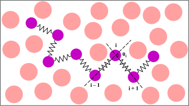
Figure 1: Schematic shows an eight unit long (N = 8) bead-spring model of a polymer (purple beads connected by black springs) in a crowed environment consisting of mobile (pink) particles. The bond angle for the $i^{th}$ bead is shown as described in Eq. (5). In the figure the diameter of the EV particles $\sigma_{part}=1.5\sigma_{poly}$.

The EV interaction between any two monomers along the chain is given by a short range Lennard-Jones (LJ) potential

$$U_{\mathrm{LJ}}(r) = 4\epsilon\left[{\left(\frac{\sigma}{r}\right)}^{12}-{\left(\frac{\sigma}{r}\right)}^{6}\right]+\epsilon,\;\mathrm{for~{}~{}}r\leq 2^{1/6}\sigma;$$ (3)

$$= 0,\;\mathrm{for~{}~{}}r>2^{1/6}\sigma.$$

Here, $\sigma=\sigma_{poly}$ is the effective diameter of a monomer on a polymer chain, and $\epsilon$ is the strength of the LJ potential. The connectivity between neighboring monomers is modeled as a FENE spring with

$$U_{\mathrm{FENE}}(r_{ij})=-\frac{1}{2}k_{F}R_{0}^{2}\ln\left(1-r_{ij}^{2}/R_{0}^{2}\right).$$ (4)

Here, $r_{ij}=\left|\vec{r}_{i}-\vec{r}_{j}\right|$ is the distance between the consecutive monomer beads $i$ and $j=i\pm 1$ at $\vec{r}_{i}$ and $\vec{r}_{j}$, $k_{F}$ is the spring constant, and $R_{0}$ is the maximum allowed separation between connected monomers. The chain stiffness $\kappa$ is introduced by adding an angle dependent three body interaction term between successive bonds as (Fig. 1)

$$U_{\mathrm{bend}}(\theta_{i})=\kappa\left(1-\cos\theta_{i}\right).$$ (5)

Here $\theta_{i}$ is the angle between the bond vectors $\vec{b}_{i-1}=\vec{r}_{i}-\vec{r}_{i-1}$ and $\vec{b}_{i}=\vec{r}_{i+1}-\vec{r}_{i}$, respectively, as shown in Fig. 1. The strength of the interaction is characterized by the bending rigidity $\kappa$ associated with the $i^{th}$ angle $\theta_{i}$. For a homopolymer chain the bulk persistence length $\ell_{p}$ of the chain in 2D and 3D are given by given by [22]

$$\ell_{p}/\sigma=2\kappa/k_{B}T\quad{\rm(2D)},$$ (6a)

$$\ell_{p}/\sigma=\kappa/k_{B}T\quad{\rm(3D)}.$$ (6b)

The additional EV particles of diameter $\sigma_{part}$ are introduced using the same short-range Lennard-Jones potential with repulsive cut-off $r_{c}=2^{1/6}\sigma_{ij}$ as in Eq. (3) with $\sigma_{ij}=\frac{\sigma_{i}+\sigma_{j}}{2}$. Here the indices $i$ and $j$ span all the polymer beads and the additional EV particles with $\sigma_{i}$ or $\sigma_{j}$ being either $\sigma_{poly}$ or $\sigma_{part}$ respectively.

We use the Langevin dynamics with the following equations of motion for the i^th monomer

$$m\ddot{\vec{r}}_{i}=-\nabla(U_{\mathrm{LJ}}+U_{\mathrm{FENE}}+U_{\mathrm{bend}}\\ +U_{\mathrm{wall}})-\Gamma\vec{v}_{i}+\vec{\eta}_{i}.$$ (7)

Here $\vec{\eta}_{i}(t)$ is a Gaussian white noise with zero mean at temperature $T$, and satisfies the fluctuation-dissipation relation in $d=2$ and 3 physical dimensions.

$$<\,\vec{\eta}_{i}(t)\cdot\vec{\eta}_{j}(t^{\prime})\,>=2dk_{B}T\Gamma\,\delta_{ij}\,\delta(t-t^{\prime}).$$ (8)

We express length and energy in units of $\sigma$ and $\epsilon$, respectively. The parameters for the FENE potential in Eq. (4), $k_{F}$ and $R_{0}$, are set to $k_{F}=30\epsilon/\sigma$ and $R_{0}=1.5\sigma$, respectively. The friction coefficient and the temperature are set to $\Gamma=0.7\sqrt{m\epsilon/\sigma^{2}}$ and $k_{B}T/\epsilon=1.2$ respectively. The force is measured in units of $k_{B}T/\sigma$. The mass of each bead for both the polymers and the EV particles is chosen to be the same.

The numerical integration of Equation (7) is implemented using the algorithm introduced by van Gunsteren and Berendsen [23]. Our previous experiences with BD simulation suggest that for a time step $\Delta t=0.01$ these parameter values produce stable trajectories over a very long period of time and do not lead to unphysical crossing of a bond by a monomer [17, 24]. The average bond length stabilizes at $b_{l}=0.971\pm 0.001$ with negligible fluctuation regardless of the chain size and rigidity [17]. We have used a Verlet neighbor list [25] instead of a link-cell list to expedite the computation. In addition, the simulation runs for the EV particles were done using LAMMPS [26] with the same potentials for numerical expediency. We have checked that these runs yield the same results.

III Results

We first present results for a single semi-flexible chain and the universal scaling properties in 2D and 3D in Sections A, B, and C. In Sections D and E we present the results for the effect of the additional EV particles.

III.1 Persistence length and end-to-end distance

First, we show the results for the universal properties of a 3D semiflexible chain. For comparison we have also shown the 2D results published earlier but with new, added data points [17].

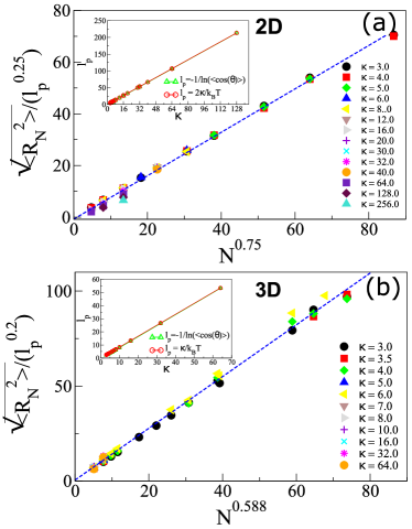
Figure 2: The scaled end-to-end distance $\sqrt{\langle R_{N}^{2}\rangle}/l_{p}^{(1/d+2)}$ as a function of $N^{\nu}$ in (a) 2D and (b) 3D. The dashed line in each figure is a straight line fit through the points. The inset in each figures shows the verification of the standard definition of persistence length (a) $\ell_{p}=2\kappa/k_{B}T$ in 2D [Eq. (6a)] and (b) $\ell_{p}=\kappa/k_{B}T$ in 3D [Eq. (6b)] in presence of the EV interaction.

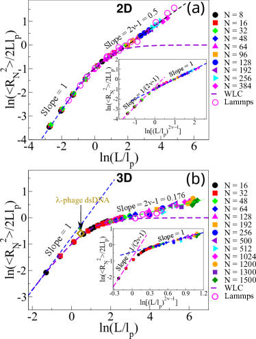
Figure 3: Log-log plot of the scaled end-to-end distances, $\langle R_{N}^{2}\rangle/2Ll_{p}$, as a function of $L/l_{p}$ for (a) 2D chains and (b) 3D chains for a variety of combinations of $L$ and $\ell_{p}$. The dashed purple line in each figure shows the behavior of the WLC model [Eq. (1)]. The insets in each figure are the plots as a function of $(L/\ell_{p})^{2\nu-1}$ those show the unit slopes for the SAW regime and clearly brings out the sharpness of the crossover in 2D and rounded narrow Gaussian regime in 3D. The symbol $\diamond$ refers to the experimental value for $\lambda$-phage dsDNA from Table I.

This is required to compare with the 2D results in the presence of the EV particles. A large number of combinations of chain lengths, $N=16-512$ for 2D systems and $N=16-1500$ for 3D systems, were chosen. A larger chain length for the 3D system was necessary to study the crossover from a Gaussian regime as discussed later. Before we show the scaling results, we would like to mention that the expression of the persistence length in Eq. (6a) and (6b) is derived for a WLC [22] but used in Eq. (2) to describe a swollen chain. The validity of the Eqs. (6a) and  (6b) and of Eq. (2) for a swollen chain in 2D and 3D are shown in Fig. 2. We rationalize the apparent contradiction by arguing that the chain persistence length is a local property of the chain calculated from the immediate three body interaction from a given bead and thus inclusion of the EV effect does not affect this result.

III.2 Universal aspects of chain conformation

Now we show the universal aspects of a swollen chain. Figs. 3(a)-(b) show the universal scaling and crossover plots in 2D and 3D respectively. First, we discuss the data collapse of the root-mean-square (RMS) end-to-end distance $\langle R_{N}^{2}\rangle$. The choice of the dimensionless $y$-axis $\langle R_{N}^{2}\rangle/2Ll_{p}$ in Figs. 3(a) and 3(b) is guided by noting that in the limit $L\gg\ell_{p}$ Eq. (1) results in $\langle R_{N}^{2}\rangle\rightarrow 2Ll_{p}$, the Gaussian limit of the WLC. Thus in the absence of the EV interaction, the quantity $\langle R_{N}^{2}\rangle/2Ll_{p}\rightarrow 1$ and would exhibit a zero slope [dashed purple line in Fig. 3(a) and (b)]. However, for $L\gg\ell_{p}$, eventually, the EV effect will become important, and from Eq. (2) it is easy to check that $\langle R_{N}^{2}\rangle\sim\left(L/\ell_{p}\right)^{2\nu-1}$. This is clearly the case as evident from Fig. 3(a)-(b) for 2D and 3D respectively. But we note that for 2D there is no Gaussian regime. For the 3D case, the Gaussian regime is very short. This trend has also been reported in the MC simulation [20] using a completely different method.

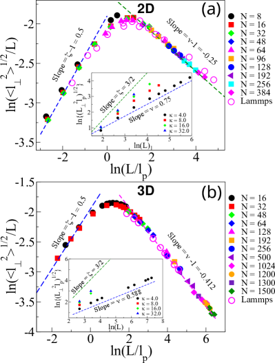
Figure 4: Log-log plot of the scaled transverse fluctuation $\sqrt{\langle l_{\perp}^{2}\rangle}/L$, as a function of $L/l_{p}$ for (a) 2D and (b) 3D chains for a variety of combinations of $L$ and $\ell_{p}$. The inset in each case shows the log-log plot of $\sqrt{L_{\perp}^{2}l_{p}}$ as a function of chain’s contour length.

III.3 Universal aspects of transverse fluctuations

We now discuss the universality in transverse fluctuation. For each configuration of the polymer chain generated during the simulation, we choose the unit vector $\hat{R}_{N}=\vec{R}_{N}/R_{N}$ as the longitudinal axis to calculate transverse fluctuations as follows:

$$\langle l_{\bot}^{2}\rangle=\frac{1}{N}\sum_{i=1}^{N}y_{i}^{2},$$ (9)

where $y_{i}$ is the perpendicular distance of the $i^{th}$ monomer with respect to the instantaneous direction $\hat{R}_{N}$. We have repeated this calculation for several chain lengths from extremely stiff chains to fully flexible chains. In the rod limit $\ell_{p}\gg L$ it can be shown that for a WLC chain the transverse fluctuation with respect to the direction of the end-to-end vector obeys the following equation

$$\langle l_{\perp}^{2}\rangle\sim L^{3}/\ell_{p}\;.$$ (10)

The transverse fluctuation in this limit of a weakly bending rod is related to the roughness exponent $\zeta$

$$\sqrt{\langle l_{\perp}^{2}\rangle}\sim L^{\zeta},$$ (11)

where $\zeta=\frac{3}{2}$ [27]-[30]. Thus, in the limit $\ell_{p}\gg L$ for an extremely stiff chain, the transverse fluctuation is governed by the roughening exponent $\langle l_{\perp}^{2}\rangle\sim L^{1.5}$, independent of the spatial dimension of the system. In the other limit of a fully flexible chain the transverse fluctuation depends on the physical dimension and is governed by the Flory exponent of the given spatial dimension as follows.

$$\langle l_{\perp}^{2}\rangle\sim L^{2\nu}.$$ (12)

These limits are shown in insets of Figs. 4(a)-(b).

We also observe that all the data in Fig. 4(a)-(b) collapses onto the same plot with the peak fluctuation around $L\approx 3\ell_{p}$. This can be understood in the following way. The transverse fluctuations go to zero in the limit of an extremely stiff chain and begin to grow as the ratio $L/\ell_{p}$ gets larger. Please note that in order for the “transverse” fluctuation to remain significant compared to the longitudinal fluctuation the chain has to be stiff enough. As the chain becomes more flexible the fluctuations start to grow in the longitudinal direction while weakening in the transverse component. We find that when $\ln(L/\ell_{p})\simeq 1$, or $L\approx 3\ell_{p}$, the transverse fluctuation becomes maximum. The limiting slopes for the $\sqrt{\langle l_{\perp}^{2}\rangle}/L$ for $L/\ell_{p}\ll 1$ and for $L/\ell_{p}\gg 1$ follow from Eqs. (11) and (12) can be written as

$$\lim_{L/\ell_{p}\rightarrow 0}\sqrt{\langle l_{\perp}^{2}\rangle}/L\sim\left(L/\ell_{p}\right)^{\zeta-1},$$ (13a)

$$\lim_{L/\ell_{p}\rightarrow\infty}\sqrt{\langle l_{\perp}^{2}\rangle}/L\sim\left(L/\ell_{p}\right)^{1-\nu}$$ (13b)

These asymptotic limits are clearly seen in Figs. 4(a)-(b) both in 2D and in 3D respectively. The simulation data fits extremely well with these predictions. The scaling relation can be used to extract either the $\ell_{p}$ or the $L$ if one or the other is known by simply adjusting the ratio $L/\ell_{p}$ (like a knob) until the point falls onto the universal plot.

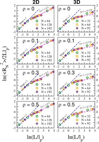
Figure 5: Log-log plot of the scaled end-to-end distances, $\langle R_{N}^{2}\rangle/2Ll_{p}$, as a function of $L/l_{p}$. The left column (2D) and the right column (3D) correspond to a variety of combinations of $L$ and $\ell_{p}$ for several different values of the densities of the crowding particles. The symbols $\circ$, $\Box$, and $\diamond$ refer to chain lengths $N=64,128$ and 192 in 2D (left column) and to the chain lengths $N=32,64$, and 92 in 3D (right column) respectively.

III.4 Effect of Crowding

Having established the universal scaling relations for the conformations and fluctuations for a single chain, we now study the effect of the EV particles on these results. The motivation comes from the living world where biopolymers such as a double stranded DNA inside a cell encounter crowded environments that affect their conformation and dynamics and hence their various functionalities. In order to check how the universal scaling relations are affected by the presence of the EV particles, we have studied chains of different lengths ($N=64-192$) in the presence of dynamic EV particles of different diameters ($\sigma_{part}=1.0\sigma,1.5\sigma$ and $2.0\sigma$) with repulsive cut-off interaction potentials as a function of the density $\rho=0.1-0.5$ (or equivalent volume fraction $\phi=\frac{1}{4}\rho\pi\sigma_{part}^{2}$ ) of the EV particles in both 2D and 3D. We have also varied the chain persistence length $\ell_{p}$ such that the ratio $L/\ell_{p}$ spans a broad range of values. First, we studied the effect of the crowding for EV particles whose diameters are the same as that of the polymer beads ($\sigma_{part}=1.0\sigma$, please refer to the Section II and Fig. 1). Then for two fixed volume fractions ($\phi=0.2356$ and $0.3927$) we studied the size effects of EV particles of different diameters $\sigma_{part}=1.0\sigma,1.5\sigma$ and $2.0\sigma$. For this part, we have carried out BD simulation in 2D only keeping the mass of the beads the same.

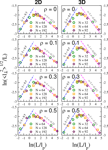
Figure 6: Log-log plot of the scaled transverse fluctuations, $\sqrt{\langle l_{\perp}^{2}\rangle}/L$, as a function of $L/l_{p}$. The symbols have the same meaning as in Fig. 5.

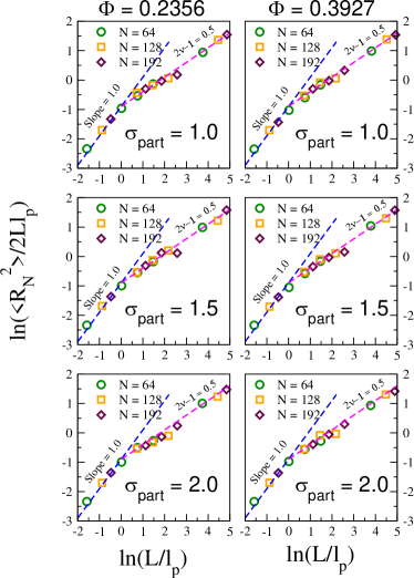
Figure 7: Log-log plot of the scaled end-to-end distances, $\langle R_{N}^{2}\rangle/2Ll_{p}$ as a function of $L/l_{p}$ in 2D for chain lengths N = 64 ($\circ$), 128 ($\Box$), and 192 ($\diamond$) for EV particle diameters of $\sigma_{part}=\sigma$, $1.5\sigma$, and $2.0\sigma$ respectively. The left and right column correspond to two volume fractions $\phi=0.2356$ and $\phi=0.3927$ of the EV particles.

III.4.1 Effect of the density of the EV particles of the same diameter

Figs. 5 and 6 show the results of the effect of the additional EV particles of the same diameter on the scaled end-to-end distance and the transverse fluctuations respectively both in 2D and in 3D. The simulations were carried out for particle densities $\rho=0.1,0.2,0.3,0.4$, and $0.5$ respectively. Only $\rho=0.1,0.3$, and $0.5$ are shown along with $\rho=0.0$ for comparison. For all of the densities studied, the data indicates that the EV particles have hardly any effect on the chain conformations and fluctuations.

III.4.2 Size effect of the EV particles of different diameters

In order to investigate how the diameters of the EV particles affect the results, additional simulations were carried out in 2D for EV particles with diameters $\sigma_{part}=1.5\sigma$ and $2.0\sigma$ respectively. We studied two volume fractions of $\phi=0.2356$ and $\phi=0.3927$. For these simulations, the mass of each EV particle remained the same. For a volume fraction of $\phi=0.2356$, the densities for $\sigma_{part}=1.0,1.5$, and 2.0 were $\rho=0.3,0.133$, and 0.075 respectively. For a volume fraction of $\phi=0.3927$, the densities for particles with $\sigma_{part}=1.0,1.5$, and 2.0 were $\rho=0.5,0.22$, and 0.125 respectively. These results are shown in Figs. 7 and 8. We find that for both the EV particle volume fraction of $\phi=0.2356$ and $\phi=0.3927$, regardless of the diameter $\sigma_{part}$ of the included EV particles, the data points for each chain tend to collapse onto the same curve. These results indicate that, for fixed EV particle volume fractions, the size of the additional EV particles that are introduced do not appear to invalidate the scaling relationships up to the maximum diameter of the EV particles that was tested.

We have further investigated the physical origin for the effect of the EV particles on the scaling laws. We have analyzed the simulation data for RMS transverse fluctuation per unit length $\langle\sqrt{l_{perp}^{2}}/L\rangle$ and noticed that this quantity ($\approx 0.1$) is at least an order of magnitude less than the average separation among the particles $\sqrt[3]{L^{3}/N}=(1.26-1.7)$ for EV particle density $\rho=(0.5–0.2)$. Thus, the presence of the particles on average hardly affects the conformations of the chain. This explains the robustness of the result.

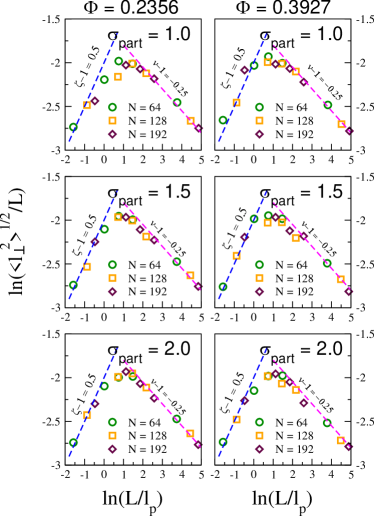
Figure 8: Log-log plot of the scaled transverse fluctuations, $\sqrt{\langle L_{\perp}^{2}\rangle}/L$, as a function of the scaled lengths, $L/l_{p}$. The symbols have the same meaning as in Fig. 7.

III.5 Comparison with experiments

Biopolymers have a wide range of flexibility. A single stranded DNA (ssDNA) is more flexible than a double stranded DNA (dsDNA). Actins and Microtubules are much more rigid. We have gathered experimental values of $L/\ell_{p}$ ([8]-[12]) in Table I and determined how they will be described (rod, Gaussian or a swollen chain) with reference to the universal scaling plot of Fig. 3. We notice that a microtubule and other synthetic stiff polymers are characterized by rods, while a 30 $\mu$m long Actin [10] filament with a persistence length of $\ell_{p}=16.7\;\mu$m falls in the Gaussian regime, while a ss-DNA [8] is described as a swollen chain. For the $\lambda$-phage dsDNA ($L=75$ nm $\ell_{p}=46.6$nm) we also have an experimental value for the mean-square end-to-end distance, ${\langle R_{N}^{2}\rangle}=3844$, nm that enables us to obtain the scaled coordinate $(L/\ell_{p},{\langle R_{N}^{2}\rangle}/2L\ell_{p})\equiv(1.61,0.55)$. This coordinate falls right onto the universal plot ($\diamond$) in Fig. 3 in the Gaussian regime and serves as a testimonial to our theory. It is worth making a comment in this context that most of the biopolymers are described as WLC. But, a large number of them will behave as swollen chains. The universal curve of Fig. 3 can be used to classify them. Fig. 4 can then be used to extract the transverse fluctuations of the chains.

Polymer	L	$l_{p}$	$ln\left(\frac{L}{l_{p}}\right)$	Regime
Microtubules [12]	28.9 $\mu$m	5.2 mm	-5.193	Rod
BCHV-PPV [11]	0.6 nm	40 nm	-4.199	Rod
BEH-PPV [11]	0.6 nm	11 nm	-2.909	Rod
MEH-PPV [11]	0.6 nm	6 nm	-2.303	Rod
Actin [10]	30 $\mu$m	16.7 $\mu$m	1.796	Gaussian
$\lambda$-phage dsDNA [9]	75 nm	46.6 nm	0.476	Gaussian
ssDNA [8]	120.4 nm	3.1 nm	3.13	SAW
	2316 nm	5.2 nm	6.61	SAW

Table 1: Experimental values of the contour length $L$ and persistence length $\ell_{p}$ of various semi-flexible bio and synthetic polymers in the bulk and their description using the scaling plot of Fig. 3(b). For the $\lambda$-phage dsDNA, $\langle R_{N}^{2}\rangle=3844$ nm [9] and falls onto the Gaussian regime of the master plot of Fig. 3(b) [the symbol $\diamond$ in Fig. 3(b)].

IV Summary and conclusion

In conclusion, we have established universal aspects of conformations and fluctuations of a semi-flexible chain by studying the scaled end-to-end distance $\langle R_{N}^{2}\rangle/2L\ell_{p}$ and the scaled transverse fluctuation $\sqrt{\langle l_{\perp}^{2}\rangle}/L$ as a function of the scaled contour length $L/\ell_{p}$ . The purpose of the choice for the former is that in the limit of a flexible chain it exhibits the characteristics of a Gaussian chain and thus the effect of the EV will become immediately observable. The purpose of the choice of the latter is that the root-mean-square fluctuation per unit length is what is important. Furthermore, the relative flexibility of the chain is measured in units of $L/\ell_{p}$ and should be the correct length unit to understand the results. Therefore, when plotted as a function of $L/\ell_{p}$ both the end-to-end distance and the transverse fluctuations collapse onto the master plots. Comparing the plots in 2D and 3D, we conclude that the Gaussian regime, though present in 3D, is very narrow. Therefore, most of the long semiflexible polymers will be characterized by a swollen chain.

The transverse fluctuations, as expected in the rod limit, are independent of the spatial dimensions and grow as $\sqrt{\langle l_{\perp}^{2}\rangle}\sim L^{3/2}$ as described by the roughening exponent $\zeta=1.5$ (Fig. 4) while in the limit of a flexible chain the fluctuation is dimension dependent and grows as $\sqrt{\langle l_{\perp}^{2}\rangle}\sim L^{\nu}$, where $\nu$ is the corresponding Flory exponent in a given dimension. We extend our previous work and observe that not only for the asymptotic limits but for all ratios of $L/\ell_{p}$ both the scaled end-to-end distance and the scaled fluctuations collapse on universal plots, indicating that the appropriate length scale to analyze the data is $L/\ell_{p}$ which brings out these universal aspects.

Moreover, we observe that crowding due to the EV particles of different volume fractions and of the same and different sizes does not change the universality of these results. We understand this by noting that the magnitudes of the scaled transverse fluctuations are much less than the average separation of the EV particles indicating that on average chain fluctuations and conformations are hardly affected by the EV particles for the densities studied here. Thus, we believe these results will be useful to calibrate and characterize both semiflexible biopolymers and synthetic polymers with respect to a universal scale. We also would like to point out that we haven’t varied the mass of the spherical particles as a function of their sizes and have not included the hydrodynamics effects in this study. Varying the mass of the spherical particles only is not likely to change the universal scaling laws as they are polymer specific and are not affected by the presence of the particles of equal mass. However, HD effects may change these results which is beyond the scope of these studies. We conclude by stating that these results can be used as references to classify properties of intrinsically disordered proteins (IDP) which remain in an extended state and whose studies have become an increasingly important and emerging field [31].

References

- [1] C-C. Lin, E. Parrish, and R. J. Composto, Macromolecules 49, 5755-5772 (2016).
- [2] XW. Huang, Y. Peng, and JH. Huang, Colloid Polym Sci 296, 689-696 (2018).
- [3] G. Chauhan, M. L. Simpson, and S. M. Abel, J. Chem. Phys. 155, 034904 (2021)
- [4] M. K. Krotova, V. V. Vasilevskaya, N. Makita, K. Yoshikawa, and A. R. Khokhlov, Phys. Rev. Lett. 105 128302 (2010).
- [5] P. G. deGennes, Scaling concepts of polymer physics (Cornell University Press, Ithaca (1979)).
- [6] J. Moukhtar, E. Fontaine, C. Faivre-Moskalenko, and A. Arneodo, Phys. Rev. Lett. 98, 178101 (2007).
- [7] J. Moukhtar, C. Faivre-Moskalenko, P. Milani, B. Audit, C. Vaillant, E. Fontaine, F. Mongelard, G. Lavorel, P. St.-Jean, P. Bouvet, F. Argout, and A. Arneodo, J. Phys. Chem. B 114, 5125 (2010).
- [8] B. Tinland, A. Pluen, J. Sturm, and G. Weill, Macromolecules 30, 5783-5765 (1997),
- [9] F. Valle, M. Favre, Paolo De Los Rios, A. Rosa, and G. Dietler, PRL 95, 158105 (2005).
- [10] A. Ott, M. Magnasco, A. Simon, A. Libchaber, Phys. Rev. E 48 R1642 (1993).
- [11] J. M. Drake, C. L. Gettinger, A. J. Heeger, and D. J. Pine. J. Chem. Phys. 101, 1673 (1994).
- [12] Jilda Nettleton, Frederick Gittes, Brian Mickey, and Jonathon Howard, The Journal of Cell Biology 120, 923-934 (1993).
- [13] M. Rubinstein and R.H. Colby, Polymer Physics (Oxford Univ. Press, 2003).
- [14] O. Kratky and G. Porod, J. Colloid Sci. 4, 35 (1949).
- [15] D.W. Schaefer, J.F. Joanny and P. Pincus, Macromolecules 13, 1280 (1980).
- [16] H. Nakanishi, J. Physique 48 979 (1987).
- [17] A. Huang, A. Bhattacharya, and K. Binder, J. Chem. 140, 214902 (2014).
- [18] A. Huang, R. Adhikari, A. Bhattacharya and K. Binder, EPL 105, 18002 (2014).
- [19] H.-P. Hsu, W. Paul. and K. Binder, EPL 95, 68004 (2011).
- [20] H-P Hsu, W. Paul, and K. Binder, EPL 92 28003 (2010).
- [21] G. S. Grest and K. Kremer, Phys. Rev. A 33, 3628(R) (1986).
- [22] L. D. Landau and E. M. Lifshitz, Statistical Physics, Part 1, 3rd ed. (Pergamon Press, 1980).
- [23] W. F. van Gunsteren and H. J. C. Berendsen, Mol. Phys. 45, 637 (1982)
- [24] A. Huang, H.-P. Hsu, A. Bhattacharya and K. Binder, J. Chem. Phys. 143, 24310 (2015).
- [25] Michael P. Allen and Dominic J. Tildessley, Computer Simulation of Liquids, 2nd edition, (Oxford University Press, 2017).
- [26] LAMMPS - a flexible simulation tool for particle-based materials modeling at the atomic, meso, and continuum scales, A. P. Thompson, H. M. Aktulga, R. Berger, D. S. Bolintineanu, W. M. Brown, P. S. Crozier, P. J. in ’t Veld, A. Kohlmeyer, S. G. Moore, T. D. Nguyen, R. Shan, M. J. Stevens, J. Tranchida, C. Trott, S. J. Plimpton, Comp Phys Comm, 271 (2022) 10817.
- [27] H. Yamakawa and M. Fujii, J. Chem. Phys. 59, 6641 (1973).
- [28] T. Odijk, Macromolecules 16, 1340 (1983).
- [29] A. Caspi, M. Elbaum, R. Granek, A. Lachish, and D. Zbaida, Phys. Rev. Lett. 80, 1106 (1998).
- [30] A.-L. Barabasi and H. E. Stanley, Fractal Concepts in Surface Growth (Cambridge University Press, 1995).
- [31] V. N. Uversky, J. R. Gillespie, and A. L. Fink, Proteins: Structure, Function, and Genetics, 41, 415-427 (2000).