Structural Adaptivity of Directed Networks

Abstract

Network structure plays a critical role in functionality and performance of network systems. This paper examines structural adaptivity of diffusively coupled, directed multi-agent networks that are subject to diffusion performance. Inspired by the observation that the link redundancy in a network may degrade its diffusion performance, a distributed data-driven neighbor selection framework is proposed to adaptively adjust the network structure for improving the diffusion performance of exogenous influence over the network. Specifically, each agent is allowed to interact with only a specific subset of neighbors while global reachability from exogenous influence to all agents of the network is maintained. Both continuous-time and discrete-time directed networks are examined. For each of the two cases, we first examine the reachability properties encoded in the eigenvectors of perturbed variants of graph Laplacian or SIA matrix associated with directed networks, respectively. Then, an eigenvector-based rule for neighbor selection is proposed to derive a reduced network, on which the diffusion performance is enhanced. Finally, motivated by the necessity of distributed and data-driven implementation of the neighbor selection rule, quantitative connections between eigenvectors of the perturbed graph Laplacian and SIA matrix and relative rate of change in agent state are established, respectively. These connections immediately enable a data-driven inference of the reduced neighbor set for each agent using only locally accessible data. As an immediate extension, we further discuss the distributed data-driven construction of directed spanning trees of directed networks using the proposed neighbor selection framework. Numerical simulations are provided to demonstrate the theoretical results.

*

1 Introduction

Reaching consensus via diffusive inter-agent interactions is an indispensable protocol for distributed estimation, control, optimization and learning on large-scale multi-agent networks Chung et al. [15], Mesbahi and Egerstedt [34], Nedic [36], Proskurnikov and Tempo [42], Barooah and Hespanha [7], Dörfler et al. [18]. The consensus problem finds its origin in examining collective animal motions as exemplified by the Vicsek model Vicsek et al. [53], Vicsek and Zafeiris [52]. In this venue, network connectivity, realized via each agent’s interactions with its nearest neighbors, is a fundamental graph-theoretic construct for the functionality and performance of networked systems Mesbahi and Egerstedt [34]Jadbabaie et al. [24], Ren et al. [44], Olfati-Saber and Murray [38], Olfati-Saber et al. [39].

In Jadbabaie et al. [24], a comprehensive analysis of the Vicsek model from the perspective of discrete-time dynamical systems was presented, where network connectivity was shown to play a critical role in reaching a consensus via local interactions. The continuous-time counterpart has also been examined in Olfati-Saber and Murray [38] for both static and dynamic networks. We note that network connectivity conditions for consensus can be further relaxed to that the underlying interaction network has a directed spanning tree Lin et al. [30], Ren et al. [44], Cao et al. [11].

Although network connectivity is critical in reaching consensus, the convergence performance (which can be characterized by the spectrum of the network matrices, e.g., Laplacian matrix for the continuous-time case and SIA (stochastic, indecomposable, and aperiodic) matrix for discrete-time case Ren et al. [44], Cao et al. [11], Olfati-Saber and Murray [38], Kim and Mesbahi [28], Clark et al. [16], Mesbahi and Egerstedt [34]) may vary considerably among a variety of connected networks. As such, a notable observation is that network connectivity often exhibits redundancies in interactions, and can hinder the diffusion performance of networks Anderson et al. [4], Blondel et al. [10], Duchi et al. [19], Nedich et al. [37], Olshevsky and Tsitsiklis [40], Shao et al. [49]. Moreover, a networked system may also suffer from performance degradation if it cannot adapt its underlying network structure to varying task objectives Song et al. [51], Kia et al. [27]. Here, a relevant question is means of designing task-oriented mechanisms that adapt the network structure to its performance demands.

This paper examines the structural adaptivity of networks, namely, how a network can adaptively alter its structure to the variation of task objectives, preferably in a distributed manner, to maintain or even enhance its performance (or functionality). Specifically, we examine structural adaptivity of networks to variations of exogenous influence (which is employed to steer the network to the desired state and can vary in both quantity and location); the performance metric we are interested in here is the convergence rate of the network state towards the exogenous influence Leonard and Fiorelli [29], Cao et al. [12], Clark et al. [16], Xia and Cao [56], Pirani and Sundaram [41].

The notion of adaptation has of course been extensively examined in disciplines such as adaptive control [5], adaptive structures in material science [54, 55], and adaptive neighbor selection in wireless communication networks [1, 9]. However, very limited works focus on how a networked system adapts its structure to the variation of task objectives. Notably, adaptive protocols were introduced to distributively manipulate the mean tracking and variance damping measures of consensus-type networks in [13], where performance measures were analyzed using an effective resistance analogy.

In order to examine the response of a diffusively coupled network to exogenous influence, the leader-following paradigm turns out to be suitable and has been widely examined in literature. In this direction, leader-follower reachability has played a critical connectivity measure, encoding information transmission from exogenous influence to agents in the network Cao et al. [12], Ji et al. [26], Liu et al. [31], Leonard and Fiorelli [29], Jadbabaie et al. [25], Alanwar et al. [2]. Unfortunately, the structure of networked systems often does not exhibit native task-oriented, efficient leader-follower reachability structures; as such the structure can degrade the network performance. Remarkably, the organization of animal groups in nature often exhibits dynamic hierarchical structures for group performance Zafeiris and Vicsek [57]. For instance, it has been observed that each bird in a avian swarm interacts only with six to seven of their nearest neighbors, rather than with all birds within its sensing radius [6]. Such observations motivate exploring suitable mechanisms to improve the performance of networked systems using structural adaptivity.

The neighbor selection operation is a convenient means for adapting the network structure to the exogenous influence potentially in a distributed manner. Notice that the network structure of large-scale network systems may not be locally accessible due to the limits of authority or privacy-preservation concerns Kia et al. [27], Lu and Zhu [32], Dibaji et al. [17]. Intuitively, inter-agent dynamics can encode graph-theoretic information on the network, and hence, may render utilizing locally accessible data collected from the network process in order to adaptively adjust the network structure feasible Shao et al. [48], Gardner et al. [21], Chiuso and Pillonetto [14], Shahrampour and Preciado [46], Nabi-Abdolyousefi and Mesbahi [35]. Recently, a distributed neighbor selection approach has been proposed for undirected networks for performance enhancement Shao et al. [50, 49]. However, directed networks are ubiquitous in real-world systems, where the asymmetry in the agents’ interaction makes their technical treatment more intricate than their undirected counterpart.

Contributions. This work proposes a distributed data-driven neighbor selection framework to enhance the structural adaptivity of diffusively coupled, directed multi-agent networks that are subject to diffusion performance of exogenous influence. The main contributions of this paper are summarized as follows.

First, distributed data-driven neighbor selection protocols for both continuous-time and discrete-time directed networks are examined. For each of the two cases, we first examine the leader-follower reachability properties encoded in eigenvectors of perturbed variants of graph Laplacian (for continuous-time case) and SIA matrix (for discrete-time case) of the underlying directed networks, respectively. Secondly, an eigenvector-based rule for neighbor selection is developed to construct a reduced network from the original one, on which the convergence rate is enhanced. Finally, as the eigenvectors are global network variables, for the purpose of distributed implementation of the neighbor selection rule, quantitative connections between eigenvectors of the perturbed graph Laplacian and SIA matrix and relative rate of change in agent state are established, respectively. Based on these connections, data-driven inference of the reduced neighbor set for each agent, using only local observations, becomes feasible. Moreover, for the case of single exogenous influence anchor, we further extend the neighbor selection framework to distributed data-driven construction of directed spanning trees contained in directed networks. To our best knowledge, distributed data-driven construction of spanning trees using network data has not previously appeared in the literature.

The contribution of this work has several immediate implications. In applications, large-scale network systems may suffer from poor responsiveness to external control. This paper provides a novel neighbor selection rule for cooperative tasks built on leader-following paradigm, making it possible to enhance the responsiveness of a network to exogenous influence by online adjustment of network structure. The graph-theoretic results in this paper also unravels the elegant leader-follower reachability property embedded in two categories of eigenvectors associated with directed networks, essentially a novel monotonicity property that was previously only investigated for Fielder vectors of undirected networks Biyikoglu et al. [8], Fiedler [20], Merris [33]. Meanwhile, this paper further extends the application scope of the distributed neighbor selection protocol from distributed averaging on undirected networks to continuous-time/discrete-time directed networks. In fact, the main results in this paper can also be extended signed directed networks Altafini [3].

The remainder of the paper is organized as follows. Notation and preliminaries are presented in $\mathsection$2. We motivate this work in $\mathsection$3, followed by the data-driven distributed neighbor selection algorithm for continuous-time and discrete-time leader-follower networks in $\mathsection$4 and $\mathsection$5, respectively. An algorithm for distributed construction of spanning tree of directed networks is presented in $\mathsection$6. Simulation results are provided in $\mathsection$7, followed by concluding remarks in $\mathsection$8.

2 Preliminaries

In this section we provide an overview on the notation and preliminary constructs used subsequently in the paper.

2.1 Notation

We let $\mathbb{R}$ and $\mathbb{Z}_{+}$ denote the set of real numbers and positive integers, respectively. Denote the set $\left\{1,2,\ldots,n\right\}$ as $\underline{n}$, where $n\in\mathbb{Z}_{+}$; $\mathds{1}_{n}$ and $0_{n\times m}$ denote $n\times 1$ vector and $n\times m$ matrix of all ones and all zeros, respectively. Let $I_{n}$ denote the $n\times n$ identity matrix and $\boldsymbol{e}_{j}$ denote the $j$th column of $I_{n}$ where $j\in\underline{n}$. Let $\text{{\bf Re}}(\cdot)$ denote the real part of a complex number. The $i$th smallest eigenvalue and the corresponding normalized eigenvector of a matrix $M\in\mathbb{R}^{n\times n}$ are signified by $\lambda_{i}(M)$ and $\boldsymbol{v}_{i}(M)$, respectively. We write $M\geq 0$ when $M$ is a non-negative matrix. The entry located at the $i$th row and $j$th column in a matrix $M\in\mathbb{R}^{n\times m}$ is denoted by $[M]_{ij}$ and the $i$th entry of a vector $\boldsymbol{x}\in\mathbb{R}^{n}$ by $[\boldsymbol{x}]_{i}$. Let $\boldsymbol{x}_{ij}$ denote $\frac{[\boldsymbol{x}]_{i}}{[\boldsymbol{x}]_{j}}$ for a vector $\boldsymbol{x}\in\mathbb{R}^{n}$. The Euclidean norm of a vector $\boldsymbol{x}\in\mathbb{R}^{n}$ is designated by $\|\boldsymbol{x}\|=(\boldsymbol{x}^{\top}\boldsymbol{x})^{\frac{1}{2}}$ . A vector $\boldsymbol{x}\in\mathbb{R}^{n}$ is positive if $[\boldsymbol{x}]_{i}>0$ for all $i\in\underline{n}$. The spectral radius of a matrix $M$ is denoted by $\text{$\rho$}(M)$. Let $\phi(\eta)=(\boldsymbol{e}_{i_{1}},\cdots,\boldsymbol{e}_{i_{s}})^{\top}\in\mathbb{R}^{s\times n}$ denote selection matrix of a set $\eta=\left\{i_{1},\ldots,i_{s}\right\}\subset\underline{n}$. The number of $k$-combinations of $\left\{1,\cdots,n\right\}$ ($n$ choose $k$) is denoted by $\left(\begin{array}[]{c}n\\ k\end{array}\right)$.

2.2 Graph Theory

Let $\mathcal{G}=(\mathcal{V},\mathcal{E},W)$ denote a graph with the node set $\mathcal{V}=\left\{1,2,\ldots,n\right\}$ and edge set $\mathcal{E\subset V\times V}$. The adjacency matrix $W=(w_{ij})\in\mathbb{R}^{n\times n}$ is such that the edge weight between agents $i$ and $j$ satisfies $w_{ij}>0$ if and only if $(i,j)\in\mathcal{E}$ and $w_{ij}=0$ otherwise. A graph $\mathcal{G}$ is undirected if $(i,j)\in\mathcal{E}$ if and only if $(j,i)\in\mathcal{E}$; otherwise $\mathcal{G}$ is directed. Denote the neighbor set of an agent $i$ as $\mathcal{N}_{i}=\left\{j\in\mathcal{V}|(i,j)\in\mathcal{E}\right\}$ and the in-degree of agent $i$ as $d_{i}=\sum_{j\in\mathcal{N}_{i}}w_{ij}$. We further denote the in-degree matrix of $\mathcal{G}$ as $D=\text{diag}\left\{d_{1},\ldots,d_{n}\right\}$. A directed path from $j\in\mathcal{V}$ to $i\in\mathcal{V}$ in a graph $\mathcal{G}$ is a concatenation of edges $\mathcal{P}_{i,j}=\{(i,i_{1}),(i_{1},i_{2}),\cdots,(i_{p-1},j)\}$, where all nodes $i,i_{1},\ldots,i_{p-1},j\in\mathcal{V}$ are distinct. A node $i\in\mathcal{V}$ is reachable from a node $j\in\mathcal{V}$ in $\mathcal{G}$ if there exists a directed path $\mathcal{P}_{i,j}$ in $\mathcal{G}$. A directed graph is strongly connected if each pair of nodes in $\mathcal{G}$ are reachable from each other. A spanning tree of a directed graph is a tree that contains all nodes in $\mathcal{G}$, denoted by $\mathcal{ST}(\mathcal{G})$. A subgraph $\mathcal{\tilde{G}}=(\tilde{\mathcal{V}},\tilde{\mathcal{E}})$ of a graph $\mathcal{G}=(\mathcal{V},\mathcal{E})$ is a graph such that $\tilde{\mathcal{V}}\subset\mathcal{V}$ and $\tilde{\mathcal{E}}\subset\mathcal{E}$. The subgraph obtained by removing a node set $\mathcal{V}^{\prime}\subset\mathcal{V}$ and all incident edges from a graph $\mathcal{G}=(\mathcal{V},\mathcal{E})$ is denoted by $\mathcal{G}-\mathcal{V}^{\prime}.$ Let $\mathcal{S}\subset\mathcal{V}$ be any subset of nodes in $\mathcal{G}=(\mathcal{V},\mathcal{E})$. Then the induced subgraph $\mathcal{G}(\mathcal{S})$ is the graph whose node set is $\mathcal{S}$ and whose edge set consists of all of the edges incident to nodes in $\mathcal{S}$.

2.3 Leader-follower Networks

We shall employ the leader-follower paradigm for characterization of how the exogenous influence been exerted on a network. Consider a leader-follower network consisting of $n\in\mathbb{Z}_{+}$ agents whose interaction structure is characterized by a directed graph $\mathcal{G}=(\mathcal{V},\mathcal{E},W)$. The state of each agent $i\in\mathcal{V}$ is denoted by $\boldsymbol{x}_{i}(t)\in\mathbb{R}$ or$\boldsymbol{x}_{i}(k)\in\mathbb{R}$ where $t$ and $k$ are time indices. In a leader-follower network, the leaders, denoted by $\mathcal{V}_{\text{L}}\subset\mathcal{V}$, can be directly influenced by the external input signals, and the remaining agents are referred to as followers, denoted by $\mathcal{V}_{\text{F}}=\mathcal{V}\setminus\mathcal{V}_{\text{L}}$. In this paper, the set of external inputs is denoted by $\mathcal{U}=\left\{u_{1},\dots,u_{m}\right\}$, where $u_{l}\in\mathbb{R}$, $l\in\underline{m}$ $(m\leq n)$. The external input $\boldsymbol{u}$ is homogeneous if $u_{i}=u_{j}$ for all $i\neq j\in\underline{m}$ and heterogeneous otherwise. In this setup, it is assumed that each leader is at most influenced by one external input and the external input $\boldsymbol{u}$ is homogeneous. The influence magnitude of the external inputs on an agent $i$ is characterized by a scalar-valued weight $\delta_{i}\geq 0$ such that $\delta_{i}>0$ if agent $i$ is a leader and $\delta_{i}=0$ if agent $i$ is a follower. Let $\boldsymbol{\delta}=\left(\delta_{1},\ldots,\delta_{n}\right)^{\top}$ denote the structure of external inputs; the set of leaders can subsequently be defined as $\mathcal{V}_{\text{L}}=\left\{i\in\mathcal{V}\thinspace|\thinspace\delta_{i}>0\right\}$.

3 A Motivational Example

Here, we provide a motivational example for this work. Consider a diffusively coupled multi-agent system (to be defined subsequently) on a strongly connected $3$-node path graph $\mathcal{G}$ shown in Figure 1. Consider two cases of leader selection in Figure 1, say $\mathcal{V}_{\mathrm{L}}=\left\{1\right\}$ (Figure 1a) and $\mathcal{V}_{\mathrm{L}}=\left\{2\right\}$ (Figure 1b), and the respective diffusion-efficient subgraphs shown in each right panel. In this context, it is relevant to ask if the network can adaptively vary according to the variations of leader set, in order to improve information diffusion. The answer to this inquiry, as shown in the paper, is affirmative. In particular, we will show that each agent can use locally observable information to adjust its in-degree neighbors, referred to as neighbor selection to improve the network performance; in this manner, the entire network exhibits adaptation to assume a diffusion-efficient structure. Moreover, we also show that the neighbor selection algorithm can be used to construct directed spanning trees in directed networks in a data-driven manner.

Figure 1: A strongly connected $3$-node path network influenced by external input $u$ through agent 1 and agent 2, respectively.

In the following discussion, we shall make the following assumptions.

Assumption 1. The underlying networks of multi-agent systems are strongly connected directed graphs.

Assumption 2. Each agent can only be directly influenced by at most one external input.

4 Continuous-time Leader-follower Networks

In this section, a distributed data-driven neighbor selection algorithm, based on the monotonicity of the eigenvector entries in the perturbed Laplacian, is proposed. Subsequently, the convergence rate of the multi-agent system on the derived reduced network, after neighbor selection, will be examined. Furthermore, the distributed implementation of the neighbor selection process will be discussed.

Consider the continuous-time leader-follower network (CLFN) whose interaction protocol for each agent $i\in\mathcal{V}$ admits the form,

$$\dot{x}_{i}(t) =-\sum_{i=1}^{n}w_{ij}(x_{i}(t)-x_{j}(t))-\sum_{l=1}^{m}b_{il}(x_{i}(t)-u_{l}),$$ (1)

where $b_{il}=\delta_{i}\neq 0$ if and only if $i$ is directly influenced by $u_{l}$ and $b_{il}=0$ otherwise. Subsequently, the overall dynamics of the CLFN (1) can be characterized as,

$$\dot{\boldsymbol{x}}=-L_{B}\boldsymbol{x}+B\boldsymbol{u},$$ (2)

where $\boldsymbol{x}=(x_{1}(t),\dots,x_{n}(t))^{\top}\in\mathbb{R}^{n}$, $B=(b_{il})\in\mathbb{R}^{n\times m}$, $\boldsymbol{u}=(u_{1},\dots,u_{m})^{\top}\in\mathbb{R}^{m}$ and

$$L_{B}=L+\text{{\bf diag}}\left\{\boldsymbol{\delta}\right\};$$ (3)

the latter matrix is referred to as perturbed Laplacian since it is obtained from a perturbation on the Laplacian matrix $L=D-W$ by a diagonal matrix. The CLFN (1) is also known as Taylor’s model in social network analysis [43].

We shall first examine the leader-follower reachability (LF-reachability) property of the CLFN (1) after the neighbor selection process. The pair $(\lambda_{\text{1}}(L_{B}),\boldsymbol{v}_{\text{1}}(L_{B}))$ associated with the perturbed Laplacian $L_{B}$ of the CLFN (1) turns out to be an important algebraic construct revealing graph-theoretic properties of CLFNs. As such, we shall unravel the network reachability, encoded in the eigenvector $\boldsymbol{v}_{\text{1}}(L_{B})$, providing useful insights for designing the neighbor selection algorithm for (1). First, we present the following critical properties of $\lambda_{\text{1}}(L_{B})$ and $\boldsymbol{v}_{\text{1}}(L_{B})$, respectively.

Lemma 1.

Let $\lambda_{1}(L_{B})$ and $\boldsymbol{v}_{1}(L_{B})$ denote the smallest eigenvalue and the corresponding normalized eigenvector of $L_{B}$ in (3), respectively. Then, $\lambda_{1}(L_{B})>0$ is a simple real eigenvalue of $L_{B}$ and $\boldsymbol{v}_{1}(L_{B})$ can be chosen to be positive.

Proof.

Let us regard the external inputs as an extra agent introduced into the network $\mathcal{G}$ and denote it as $u$. Moreover, let us denote the edge set between external inputs and the leaders as $\mathcal{E}^{{}^{\prime}}$. We consider the augmented directed network $\widehat{\mathcal{G}}=(\widehat{\mathcal{V}},\widehat{\mathcal{E}},\widehat{W})$ such that $\widehat{\mathcal{V}}=\mathcal{V}\cup\left\{u\right\}$, $\widehat{\mathcal{E}}=\mathcal{E}\cup\mathcal{E}^{{}^{\prime}}$ and $\widehat{W}=\left(\begin{array}[]{cc}W&\boldsymbol{\delta}\\ 0_{1\times n}&0\end{array}\right)$. Then the Laplacian matrix of $\widehat{\mathcal{G}}$ is $\widehat{L}=\left(\begin{array}[]{cc}L_{B}&-B\mathds{1}_{m}\\ 0_{1\times n}&0\end{array}\right)$. Therefore, all eigenvalues of $L_{B}$ are eigenvalues of $\widehat{L}$. Since $\widehat{\mathcal{G}}$ has a directed spanning tree with the root $u$, then $\widehat{L}$ has only one zero eigenvalue with all other eigenvalues having positive real parts, i.e., $\text{{\bf Re}}(\lambda_{\text{1}}(L_{B}))>0$.

We now proceed to show that $\lambda_{\text{1}}(L_{B})$ is a simple real eigenvalue and $\boldsymbol{v}_{\text{1}}(L_{B})$ can be chosen to be positive. Let $L_{B}=\eta I-M$, where $M\in\mathbb{R}^{n\times n}$ is a non-negative matrix and $\eta={\displaystyle\max_{i\in\underline{n}}}\left\{[L_{B}]_{ii}\right\}$. Then $e^{-L_{B}}=e^{M-\eta I}=e^{-\eta I}e^{M}$. Note that the matrix $M$ is non-negative, therefore, $e^{-L_{B}}$ is a non-negative matrix. In addition, since the network $\mathcal{G}$ is strongly connected, $M$ is irreducible, implying that $e^{-L_{B}}$ is a non-negative irreducible matrix. Thus, according to Perron–Frobenius theorem Horn and Johnson [23], the eigenvalue $e^{-\lambda_{1}(L_{B})}$ is simple and real and the corresponding eigenvector $\boldsymbol{v}_{1}(L_{B})$ can be chosen to be positive. ∎

Remark 1.

Note that the influence magnitude $\delta_{i}$ associated with the external input on an agent $i\in\mathcal{V}$ is arbitrary. Therefore Lemma 1 still holds for those graph Laplacians with arbitrary positive diagonal perturbation.

For a CLFN $\mathcal{G}$ with the input matrix $B$, we proceed to construct a reduced network of $\mathcal{G}$ by eliminating a subset of edges between specific agents and their neighboring agents, namely, neighbor selection, using information encoded in $\boldsymbol{v}_{\text{1}}(L_{B})$. We will refer to this class of reduced networks as the following the slower neighbor (FSN) networks of $\mathcal{G}$ Shao et al. [49], since it is implied that each agent follows (or chooses to be influenced by) those neighbors whose rate of change in states are relatively slower. This terminology will be made more rigorous subsequently.

Definition 1 (FSN network for CLFN).

Consider the CLFN (2) on a strongly connected directed network $\mathcal{G}=(\mathcal{V},\mathcal{E},W)$. The FSN network of $\mathcal{G}$, denoted by $\bar{\mathcal{G}}=(\mathcal{\bar{V}},\bar{\mathcal{E}},\bar{W})$, is such that $\mathcal{\bar{V}}=\mathcal{V}$, $\mathcal{\bar{E}}\subset\mathcal{E}$ and $\bar{W}=(\bar{w}_{ij})\in\mathbb{R}^{n\times n}$, where $\bar{w}_{ij}=w_{ij}$ if $\boldsymbol{v}_{\text{1}}(L_{B})_{ij}>1$ and $\bar{w}_{ij}=0$ if $\boldsymbol{v}_{\text{1}}(L_{B})_{ij}\leq 1$.

Remark 2.

Equivalently, Definition 2 implies a neighbor selection process using the information $\boldsymbol{v}_{\text{1}}(L_{B})_{ij}$, where $i$ and $j$ are neighboring agents. One notes that $\boldsymbol{v}_{\text{1}}(L_{B})$ is network-level information that is usually not accessible to local agents. However, as we shall show in §4.3, $\boldsymbol{v}_{\text{1}}(L_{B})_{ij}$ is locally computable using the relative rate of change in state between neighboring agents.

4.1 Reachability Analysis of FSN Networks

The following result reveals the LF-reachability encoded in the $\boldsymbol{v}_{\text{1}}(L_{B})$ of a CLFN.

Theorem 1 (LF-reachability).

Let $\bar{\mathcal{G}}$ be the FSN network of the CLFN (2) on a strongly connected directed network $\mathcal{G}$. Then all agents are reachable from external inputs in $\bar{\mathcal{G}}$.

Proof.

It is sufficient to show that for an arbitrary $i\in\mathcal{V}_{\text{F}}$, there exists a leader agent $l\in\mathcal{V}_{\text{L}}$ such that $i$ is reachable from $l$.

By contradiction, assume that there exists a subset of agents $\left\{i_{1},i_{2},\cdots,i_{s}\right\}\subset\mathcal{V}_{\text{F}}$ in the FSN network $\bar{\mathcal{G}}$ such that $i_{k}$ is not reachable from any $l\in\mathcal{V}_{\text{L}}$, where $k\in\underline{s}$ and $s\in\mathbb{Z}_{+}$. Let $\lambda_{1}$ be the smallest eigenvalue of the perturbed Laplacian matrix $L_{B}$ with the corresponding eigenvector $\boldsymbol{v}_{1}$, i.e.,

$$L_{B}\boldsymbol{v}_{1}=\lambda_{1}\boldsymbol{v}_{1}.$$ (4)

According to Lemma 1, one has $\lambda_{1}>0$ and the corresponding eigenvector $\boldsymbol{v}_{1}$ is positive. Now let

$$[\boldsymbol{v}_{1}]_{i^{0}}=\underset{k\in\left\{i_{1},i_{2},\cdots,i_{s}\right\}}{\mathbf{\mathbf{\min}}}\left\{[\boldsymbol{v}_{1}]_{k}\right\}.$$ (5)

Then, according to Definition 1, one has $[\boldsymbol{v}_{1}]_{j}\geq[\boldsymbol{v}_{1}]_{i^{0}}$ for all $j\in\mathcal{N}_{i^{0}}$. Examining the $i^{0}$th row in (4) yields,

$$\left({\displaystyle\sum_{j\in\mathcal{N}_{i^{0}}}}w_{i^{0}j}\right)[\boldsymbol{v}_{1}]_{i^{0}}-{\displaystyle\sum_{j\in\mathcal{N}_{i^{0}}}}w_{i^{0}j}[\boldsymbol{v}_{1}]_{j}=\lambda_{1}[\boldsymbol{v}_{1}]_{i^{0}}.$$ (6)

Combining (5) and (6), now yields the following inequality,

$$\left({\displaystyle\sum_{j\in\mathcal{N}_{i^{0}}}}w_{i^{0}j}\right)[\boldsymbol{v}_{1}]_{i^{0}}-{\displaystyle\sum_{j\in\mathcal{N}_{i^{0}}}}w_{i^{0}j}[\boldsymbol{v}_{1}]_{i^{0}}\geq\lambda_{1}[\boldsymbol{v}_{1}]_{i^{0}}.$$ (7)

By canceling $[\boldsymbol{v}_{1}]_{i^{0}}>0$ from both sides of the above inequality, one can obtain $\lambda_{1}\leq 0$, establishing a contradiction. ∎

It turns out that the entries of the eigenvector $\boldsymbol{v}_{1}(L_{B})$ are influenced by the selection of leader agents; we shall provide examples in simulation results to illustrate this point– the reader is referred to §7.3.

4.2 Convergence Rate Analysis of FSN Networks

In order to evaluate the performance of the neighbor selection process based on $\boldsymbol{v}_{\text{1}}(L_{B})$, we now proceed to examine the convergence rate of the CLFN (2) on its FSN networks. Note that the smallest non-zero eigenvalue of the perturbed Laplacian $L_{B}$ characterizes the convergence rate of the CLFN (2) towards its steady-state, either consensus or clustering [16, 56, 41]. We provide the following result regarding the relation between the convergence rate of the CLFN (2) on strongly connected directed networks and that on their FSN networks. Without loss of generality, we assume that $\delta_{i}=\delta_{j}$ for all $i,j\in\mathcal{V}_{\text{L}}$.

We first need the following results for our subsequent analysis.

Lemma 2.

Horn and Johnson [23] Let $A=\left(a_{ij}\right)\in\mathbb{R}^{n\times n}$ be a nonnegative matrix. Then $\rho(A)\leq\underset{i\in\underline{n}}{\mathbf{max}}\sum_{j=1}^{n}a_{ij}$; when all the row sums of $A$ are equal, then equality holds.

Lemma 3.

Consider the CLFN (2) on a strongly connected directed network $\mathcal{G}=(\mathcal{V},\mathcal{E},W)$. If $\mathcal{V}_{\text{\text{F}}}\not=\emptyset$, then there exists at least one edge $(i,j)\in\mathcal{E}$ such that $[\boldsymbol{v}_{1}(L_{B})]_{j}>[\boldsymbol{v}_{1}(L_{B})]_{i}$.

Proof.

In the proof, we shall use $\boldsymbol{v}_{1}$ instead of $\boldsymbol{v}_{1}(L_{B})$ for brevity. Assume that all the edges $(i,j)\in\mathcal{E}$ satisfy $[\boldsymbol{v}_{1}]_{j}\leq[\boldsymbol{v}_{1}]_{i}$. $\mathcal{V}_{\text{\text{F}}}\not=\emptyset$ implies that $\alpha\mathds{1}_{n}$ is not an eigenvector of $L_{B}$ for any non-zero scalar $\alpha\in\mathbb{R}$, therefore there exists at least one edge $(i^{\prime},j^{\prime})\in\mathcal{E}$ satisfying $[\boldsymbol{v}_{1}]_{j^{\prime}}<[\boldsymbol{v}_{1}]_{i^{\prime}}$. Since $\mathcal{G}$ is strongly connected, there exists a directed path that starts from $i^{\prime}$ and ends at $j^{\prime}$, as such, one has $[\boldsymbol{v}_{1}]_{i^{\prime}}\leq[\boldsymbol{v}_{1}]_{j^{\prime}}$, thus establishing a contradiction. Hence, there exists at least one edge $(i,j)\in\mathcal{E}$ such that $[\boldsymbol{v}_{1}]_{j}>[\boldsymbol{v}_{1}]_{i}$. ∎

We proceed to present the result regarding the performance enhancement of CLFN (2) after the neighbor selection process.

Theorem 2 (Convergence rate).

Let $\bar{\mathcal{G}}=(\mathcal{V},\mathcal{\bar{E}},\bar{W})$ denote the FSN network of CLFN (2). Then

$$\lambda_{1}(L_{B}(\bar{\mathcal{G}}))\geq\lambda_{1}(L_{B}(\mathcal{G})),$$ (8)

where equality holds if and only if all agents are leaders.

Proof.

Let $H=\left(H_{ij}\right)\in\mathbb{R}^{n\times n}=\beta I-L_{B}(\mathcal{G})$ and $\bar{H}=\left(\bar{H}_{ij}\right)\in\mathbb{R}^{n\times n}=\beta I-L_{B}(\bar{\mathcal{G}})$, where $\beta$ is a sufficiently large positive constant. Then $H$ and $\bar{H}$ are irreducible nonnegative matrices. Notice that $\rho(H)=\beta-\lambda_{1}(L_{B}(\mathcal{G}))$ and $\rho(\bar{H})=\beta-\lambda_{1}(L_{B}(\bar{\mathcal{G}}))$, it sufficient to show that $\rho(H)\geq\rho(\bar{H})$. Denote by $\varDelta=\left(\varDelta_{ij}\right)\in\mathbb{R}^{n\times n}=L_{B}(\mathcal{G})-L_{B}(\bar{\mathcal{G}})$; then ${\displaystyle\varDelta_{ij}}\leq 0$ for $i\neq j$ and ${\displaystyle\varDelta_{ii}}=-{\displaystyle\sum_{j\in\mathcal{N}_{i}}\varDelta_{ij}}$. Therefore, for all $i,j\in\underline{n},$

$$\bar{H}_{ii}=H_{ii}-{\displaystyle\sum_{j\in\mathcal{N}_{i}}\varDelta_{ij}},$$

and

$$\bar{H}_{ij}=H_{ij}+{\displaystyle\varDelta_{ij}}.$$

Let $S=\mathbf{diag}\left\{\boldsymbol{v}_{1}(L_{B})\right\}$ and thereby,

$$S^{-1}\bar{H}S=\left(\bar{H}_{ij}\frac{[\boldsymbol{v}_{1}(L_{B})]_{j}}{[\boldsymbol{v}_{1}(L_{B})]_{i}}\right)\in\mathbb{R}^{n\times n}$$

and $\rho\left(S^{-1}\bar{H}S\right)=\rho\left(\bar{H}\right)$. According to Lemma 2,

$$\rho\left(S^{-1}\bar{H}S\right)\leq\underset{i\in\underline{n}}{\mathbf{max}}\frac{1}{[\boldsymbol{v}_{1}(L_{B})]_{i}}\sum_{j=1}^{n}\bar{H}_{ij}[\boldsymbol{v}_{1}(L_{B})]_{j}.$$

Due to the fact that, for all $i\in\underline{n}$,

$$\frac{1}{[\boldsymbol{v}_{1}(L_{B})]_{i}}\sum_{j=1}^{n}\bar{H}_{ij}[\boldsymbol{v}_{1}(L_{B})]_{j}$$

$$= \left(H_{ii}-{\displaystyle\sum_{j\in\mathcal{N}_{i}}\varDelta_{ij}}\right)$$

$$+ {\displaystyle\sum_{j=1,j\neq i}^{n}\frac{\left(H_{ij}+{\displaystyle\varDelta_{ij}}\right)[\boldsymbol{v}_{1}(L_{B})]_{j}}{[\boldsymbol{v}_{1}(L_{B})]_{i}}},$$

$$= H_{ii}+\sum_{j=1,j\neq i}^{n}\frac{H_{ij}[\boldsymbol{v}_{1}(L_{B})]_{j}}{[\boldsymbol{v}_{1}(L_{B})]_{i}}$$

$$+ \sum_{j=1,j\neq i}^{n}\frac{{\displaystyle\varDelta_{ij}}[\boldsymbol{v}_{1}(L_{B})]_{j}}{[\boldsymbol{v}_{1}(L_{B})]_{i}}-{\displaystyle\sum_{j=1,j\neq i}^{n}\varDelta_{ij}}.$$

Since $\varDelta_{ij}<0$ implies $\frac{[\boldsymbol{v}_{1}(L_{B})]_{j}}{[\boldsymbol{v}_{1}(L_{B})]_{i}}\geq 1$, then one has,

$$\sum_{j=1,j\neq i}^{n}\frac{{\displaystyle\varDelta_{ij}}[\boldsymbol{v}_{1}(L_{B})]_{j}}{[\boldsymbol{v}_{1}(L_{B})]_{i}}-{\displaystyle\sum_{j=1,j\neq i}^{n}\varDelta_{ij}}\leq 0.$$

Thus, for all $i\in\underline{n}$,

$$\frac{1}{[\boldsymbol{v}_{1}(L_{B})]_{i}}\sum_{j=1}^{n}\bar{H}_{ij}[\boldsymbol{v}_{1}(L_{B})]_{j} \leq\frac{1}{[\boldsymbol{v}_{1}(L_{B})]_{i}}\sum_{j=1}^{n}H_{ij}[\boldsymbol{v}_{1}(L_{B})]_{j}$$

$$=\rho(H),$$

which implies that $\rho(\bar{H})\leq\rho(H)$.

In the following, we will further analyze the condition under which $\rho(\bar{H})=\rho(H)$. There are two cases to consider.

Case 1: the follower set is not empty. According to Lemma 3, there exists at least one edge $(i^{\prime},j^{\prime})\in\mathcal{E}$ such that $[\boldsymbol{v}_{1}(L_{B})]_{j^{\prime}}>[\boldsymbol{v}_{1}(L_{B})]_{i^{\prime}}$. Therefore,

$$\sum_{j=1,j\neq i^{\prime}}^{n}\frac{{\displaystyle\varDelta_{i^{\prime}j}}[\boldsymbol{v}_{1}(L_{B})]_{j}}{[\boldsymbol{v}_{1}(L_{B})]_{i^{\prime}}}-{\displaystyle\sum_{j=1,j\neq i^{\prime}}^{n}\varDelta_{i^{\prime}j}}<0,$$

that is,

$$\frac{1}{[\boldsymbol{v}_{1}(L_{B})]_{i^{\prime}}}\sum_{j=1}^{n}\bar{H}_{i^{\prime}j}[\boldsymbol{v}_{1}(L_{B})]_{j}<\frac{1}{[\boldsymbol{v}_{1}(L_{B})]_{i^{\prime}}}\sum_{j=1}^{n}H_{i^{\prime}j}[\boldsymbol{v}_{1}(L_{B})]_{j}.$$

Hence, if all row sums of $S^{-1}\bar{H}S$ are equal, according to Lemma 2, one has,

$$\rho(\bar{H}) = \frac{1}{\left[\boldsymbol{v}_{1}(L_{B})\right]_{i}}\sum_{j=1}^{n}\bar{H}_{ij}\left[\boldsymbol{v}_{1}(L_{B})\right]_{j}$$

$$< \frac{1}{\left[\boldsymbol{v}_{1}(L_{B})\right]_{i}}\sum_{j=1}^{n}H_{ij}\left[\boldsymbol{v}_{1}(L_{B})\right]_{j}=\rho(H)$$

for any $i\in\underline{n}$. Otherwise, if not all row sums of $S^{-1}\bar{H}S$ are equal, by Lemma 2again, we have,

$$\rho(\bar{H})<\underset{i\in\underline{n}}{\mathbf{max}}\frac{1}{\left[\boldsymbol{v}_{1}(L_{B})\right]_{i}}\sum_{j=1}^{n}\bar{H}_{ij}\left[\boldsymbol{v}_{1}(L_{B})\right]_{j}\leq\rho(H).$$

Therefore, one can conclude that,

$$\rho(\bar{H})<\rho(H).$$

Case 2: the follower set is empty. Then $\boldsymbol{v}_{1}(L_{B})=\alpha\boldsymbol{1}_{n}$ ($\alpha\in\mathbb{R}$ and $\alpha\not=0$). Moreover, for any $i\in\underline{n}$, one has,

$$\sum_{j=1,j\neq i}^{n}\frac{{\displaystyle\varDelta_{ij}}[\boldsymbol{v}_{1}(L_{B})]_{j}}{[\boldsymbol{v}_{1}(L_{B})]_{i}}-{\displaystyle\sum_{j=1,j\neq i}^{n}\varDelta_{ij}}=0.$$

Hence,

$$\frac{1}{[\boldsymbol{v}_{1}(L_{B})]_{i}}\sum_{j=1}^{n}\bar{H}_{ij}[\boldsymbol{v}_{1}(L_{B})]_{j} =\frac{1}{[\boldsymbol{v}_{1}(L_{B})]_{i}}\sum_{j=1}^{n}H_{ij}[\boldsymbol{v}_{1}(L_{B})]_{j}$$

$$=\rho(H),$$

for any $i\in\underline{n}$. Then, one can immediately conclude that $\rho(\bar{H})=\rho(H)$.

Therefore, $\lambda_{1}(L_{B}(\bar{\mathcal{G}}))\geq\lambda_{1}(L_{B}(\mathcal{G}))$ and the equality holds if only if all agents are leaders. The proof is finished. ∎

Remark 3.

Theorem 2 indicates that the convergence rate of CLFN (2) on the FSN networks outperforms the original strongly connected directed networks. In other words, the CLFN (2) enhances the network performance by adapting the network structure to the exogenous influence via neighbor selection.

4.3 Distributed Implementation of Neighbor Selection

Thus far, we have presented a neighbor selection framework with guaranteed performance using the eigenvector of the perturbed Laplacian. However, this eigenvector is a network-level quantity, hindering the direct applicability of the proposed method for large-scale networks. For such networks, it is often desired (if not necessary) that decision-making rely on local observations.

In this section, we establish a quantitative link between the eigenvector of the perturbed Laplacian and the relative rate of change in the state of neighboring agents, referred to as the relative tempo. Then, we connect the global property of the network to a locally accessible quantity, leading to a fully distributed data-driven neighbor selection algorithm.

We now proceed to introduce the notion of relative tempo, characterizing the steady-state of the relative rate of change in state between two subsets of agents.

Definition 2.

Let $\mathcal{V}_{1}\subset\mathcal{V}$ and $\mathcal{V}_{2}\subset\mathcal{V}$ be two subsets of agents in the CLFN (2). Then the relative tempo between agents in $\mathcal{V}_{1}$ and $\mathcal{V}_{2}$ is defined as,

$$\text{$\mathbb{L}$}^{c}(\mathcal{V}_{1},\mathcal{V}_{2})=\lim_{t\rightarrow\infty}\frac{\|\phi(\mathcal{V}_{1})\dot{\boldsymbol{x}}(t)\|}{\|\phi(\mathcal{V}_{2})\dot{\boldsymbol{x}}(t)\|},$$ (9)

where $\phi(\mathcal{V}_{1})$ and $\phi(\mathcal{V}_{2})$ are selection matrices associated with $\mathcal{V}_{1}$ and $\mathcal{V}_{2}$, respectively.

The relative tempo in Definition 2 was initially examined in [47], characterizing the relative influence of agents in consensus-type networks, and subsequently employed to construct a centrality measure that can be inferred from network data [48]. This paper provides a systematic treatment of the application of relative tempo in the distributed neighbor selection problem on directed networks. First, we proceed to formally provide a quantitative connection between relative tempo and the Laplacian eigenvector.

Theorem 3.

Let $\mathcal{V}_{1}\subset\mathcal{V}$ and $\mathcal{V}_{2}\subset\mathcal{V}$ be two subsets of agents in the CLFN (2). Then

$$\text{$\mathbb{L}$}^{c}(\mathcal{V}_{1},\mathcal{V}_{2})=\frac{\|\phi(\mathcal{V}_{1})\boldsymbol{v_{1}}(L_{B})\|}{\|\phi(\mathcal{V}_{2})\boldsymbol{v_{1}}(L_{B})\|}.$$

Proof.

Denote by $\phi(\mathcal{V}_{1})=\phi_{1}$ and $\phi(\mathcal{V}_{2})=\phi_{2}$ for simplicity. Without loss of generality, let us regard the external inputs as one extra input $u$. Denote $\boldsymbol{y}=\left(\begin{array}[]{cc}\boldsymbol{x}^{\top}&u\end{array}\right)^{\top}$, then $\boldsymbol{x}\left(t\right)=\left(\begin{array}[]{cc}I_{n}&0_{n\times 1}\end{array}\right)\boldsymbol{y}\left(t\right)$ and the CLFN (2) can be characterized as $\dot{\boldsymbol{y}}(t)=A\boldsymbol{y}(t)$, where $A=\left(\begin{array}[]{cc}-L_{B}&B\mathds{1}_{m}\\ 0_{1\times n}&0\end{array}\right)$. Let $\tilde{\lambda}_{p}\leq\tilde{\lambda}_{p-1}\leq\cdots\leq\tilde{\lambda}_{1}=0$ denote the distinct ordered eigenvalues of $A$, whose algebraic multiplicity is denoted by $n_{i}$ where $p\leq n+1$ and $i\in\underline{p}$. Let $J$ be the Jordan canonical form associate with $A$, i.e., $A=SJS^{-1}$, where $S=\left(\boldsymbol{\varphi}_{1},\boldsymbol{\varphi}_{2},\ldots,\boldsymbol{\varphi}_{n+1}\right)\in\mathbb{R}^{\left(n+1\right)\times\left(n+1\right)}$ and $J=\text{{\bf diag}}\left\{J(\tilde{\lambda}_{1}),J(\tilde{\lambda}_{2}),\ldots,J(\tilde{\lambda}_{p})\right\}\in\mathbb{R}^{\left(n+1\right)\times\left(n+1\right)}$. According to the solution to the matrix ordinary differential equation $\dot{\boldsymbol{y}}(t)=A\boldsymbol{y}(t)$, the time derivative of $\boldsymbol{y}(t)$ is,

$$\dot{\boldsymbol{y}}(t) =Ae^{At}\boldsymbol{y}(0)=SJe^{Jt}S^{-1}\boldsymbol{y}(0);$$ (10)

therefore, one has,

$$\|\phi_{q}\dot{\boldsymbol{x}}(t)\|^{2}= \left(\dot{\boldsymbol{x}}(t)\right)^{\top}\phi_{q}^{\top}\phi_{q}\dot{\boldsymbol{x}}(t)$$

$$= \left(\dot{\boldsymbol{y}}(t)\right)^{\top}\left(\begin{array}[]{c}I_{n}\\ 0_{1\times n}\end{array}\right)\phi_{q}^{\top}\phi_{q}\left(\begin{array}[]{cc}I_{n}&0_{n\times 1}\end{array}\right)\dot{\boldsymbol{y}}(t)$$ (14)

$$= \boldsymbol{y}(0)^{\top}(S^{-1})^{\top}e^{J^{\top}t}J^{\top}S^{\top}\tilde{\phi}_{q}^{\top}\tilde{\phi}_{q}SJe^{Jt}S^{-1}\boldsymbol{y}(0),$$ (15)

where $q\in\underline{2}$ and $\tilde{\phi}_{q}=\phi_{q}\left(\begin{array}[]{cc}I_{n}&0_{n\times 1}\end{array}\right)$.

Denote $\boldsymbol{\alpha}_{qi}=\tilde{\phi}_{q}\boldsymbol{\varphi}_{i}$ and $\boldsymbol{\beta}=\left(\beta_{1},\beta_{2},\ldots,\beta_{n+1}\right)^{\top}=S^{-1}\boldsymbol{y}(0)\in\mathbb{R}^{n+1}$ for $q\in\underline{2}$ and $i\in\underline{n+1}$. By analyzing (15), we have,

$$\tilde{\phi}_{q}SJe^{Jt}S^{-1}\boldsymbol{y}(0)$$

$$= \left(\begin{array}[]{c}\boldsymbol{\alpha}_{q1},\ldots,\boldsymbol{\alpha}_{q(n+1)}\end{array}\right)$$

$$\text{{\bf diag}}\left\{J(\tilde{\lambda}_{1}),\ldots,J(\tilde{\lambda}_{p})\right\}$$

$$\text{{\bf diag}}\left\{e^{J(\tilde{\lambda}_{1})t},\ldots,e^{J(\tilde{\lambda}_{p})t}\right\}\left(\begin{array}[]{c}\beta_{1}\\ \vdots\\ \beta_{n+1}\end{array}\right),$$

$$= {\displaystyle\sum_{k=1}^{p}}\left(\sum_{i=q_{k-1}+1}^{q_{k}}\left(\sum_{j=0}^{q_{k}-i}\frac{t^{j}}{j!}\beta_{i+j}\tilde{\lambda}_{k}+\sum_{j=1}^{q_{k}-i}\beta_{i+j}\right)\boldsymbol{\alpha}_{qi}\right)e^{\tilde{\lambda}_{k}t},$$

where $q_{k}=\sum_{h=0}^{k}n_{h}$ and $n_{0}=0$.

Now, let us denote

$$f_{1,p}(q)={\displaystyle\sum_{k=1}^{p}}\left(\sum_{i=q_{k-1}+1}^{q_{k}}\left(\sum_{j=0}^{q_{k}-i}\frac{t^{j}}{j!}\beta_{i+j}\tilde{\lambda}_{k}+\sum_{j=1}^{q_{k}-i}\beta_{i+j}\right)\boldsymbol{\alpha}_{qi}\right)e^{\tilde{\lambda}_{k}t}.$$ (18)

Then one has,

$$\|\phi_{q}\dot{\boldsymbol{x}}(t)\|^{2}$$

$$= f_{1,p}^{\top}(q)f_{1,p}(q)$$

$$= \lambda_{2}^{2}\beta_{2}^{2}e^{2\tilde{\lambda}_{2}t}\boldsymbol{\alpha}_{q2}^{\top}\boldsymbol{\alpha}_{q2}+2\lambda_{2}\beta_{2}e^{\tilde{\lambda}_{2}t}\boldsymbol{\alpha}_{q2}^{\top}f_{3,p}(q)+f_{3,p}^{\top}(q)f_{3,p}(q),$$ (19)

where,

$$f_{3,p}(q)={\displaystyle\sum_{k=3}^{p}}\left(\sum_{i=q_{k-1}+1}^{q_{k}}\left(\sum_{j=0}^{q_{k}-i}\frac{t^{j}}{j!}\beta_{i+j}\tilde{\lambda}_{k}+\sum_{j=1}^{q_{k}-i}\beta_{i+j}\right)\boldsymbol{\alpha}_{qi}\right)e^{\tilde{\lambda}_{k}t}.$$

Hence, by straightforward computation, we have,

$$\lim_{t\rightarrow\infty}\frac{\|\phi_{1}\dot{\boldsymbol{x}}(t)\|}{\|\phi_{2}\dot{\boldsymbol{x}}(t)\|}=\left(\frac{\boldsymbol{\alpha}_{12}^{\top}\boldsymbol{\alpha}_{12}}{\boldsymbol{\alpha}_{22}^{\top}\boldsymbol{\alpha}_{22}}\right)^{\frac{1}{2}}=\frac{\|\phi_{1}\boldsymbol{v_{1}}(L_{B})\|}{\|\phi_{2}\boldsymbol{v_{1}}(L_{B})\|}.$$ (20)

The statement of the lemma now follows by following a few straightforward steps, that have been omitted for brevity. ∎

Remark 4.

Theorem 3 provides a quantitative connection between the relative tempo (constructed from local observations of each agent) and the Laplacian eigenvector of the underlying network. According to Theorem 1 and Theorem 2, such a connection enables a distributed implementation of neighbor selection for enhancing the convergence rate of the network.

We shall provide illustrative examples for Theorem 3 in §7.

Remark 5.

After the neighbor selection process, each agent has an updated reduced neighbor set. The reduced neighbor set for agent $i\text{$\in\mathcal{V}$}$ in order to construct the FSN network for the CLFN (2) is,

$$\mathcal{N}_{i}^{\text{FSN}} =\left\{j\in\mathcal{N}_{i}\mid\boldsymbol{v}_{\text{1}}(L_{B})_{ij}>1\right\}$$ (21)

$$=\left\{j\in\mathcal{N}_{i}\mid\text{$\mathbb{L}$}^{c}(i,j)>1\right\},$$ (22)

where (21) and (22) characterize $\mathcal{N}_{i}^{\text{FSN}}$ from the perspectives of Laplacian eigenvector and relative tempo, respectively.

5 Discrete-time Leader-follower Networks

In the following, we shall present the parallel results for discrete-time case where the technical treatment relies on non-negative matrix analysis Seneta [45]. In a discrete-time leader-follower network (DLFN), the individual dynamics is represented as,

$$x_{i}(k+1)=p_{ii}x_{i}(k)+\sum_{j=1,j\neq i}^{n}p_{ij}x_{j}(k)+\sum_{l=1}^{m}q_{il}u_{l},\ i\in\mathcal{V},$$ (23)

where $p_{ij}=\frac{w_{ij}}{\delta_{i}+d_{i}}$ for $(i,j)\in\mathcal{E}$ and $p_{ij}=0$ otherwise; $q_{il}=\frac{\delta_{i}}{\delta_{i}+d_{i}}$ if $i\in\mathcal{V}_{\text{L}}$ and $q_{il}=0$ otherwise. Here we assume that $w_{ii}\neq 0$ for each agent $i\in\mathcal{V}_{\text{}}$. The DLFN (23) can also be considered as the consensus dynamics influenced by stubborn agents [22]. One can also find the analog in absorbing Markov chains, where a constant input can be modeled as the absorbing state [45].

The overall dynamics of (23) admits the form,

$$\boldsymbol{x}(k+1)=P\boldsymbol{x}(k)+Q\boldsymbol{u},$$ (24)

where $\boldsymbol{u}=\left(u_{1},\ldots,u_{m}\right)^{\top}$, $P=\left(p_{ij}\right)\in\mathbb{R}^{n\times n}$, and $Q=(q_{il})\in\mathbb{R}^{n\times m}$. Note that $P=(D+\text{diag}\left\{\boldsymbol{\delta}\right\})^{-1}W$ can be viewed as a diagonal matrix perturbation on the SIA matrix $D^{-1}W$ via $\text{diag}\left\{\boldsymbol{\delta}\right\}$ [11, 44]. Denote $\boldsymbol{y}=\left(\begin{array}[]{cc}\boldsymbol{x}^{\top}&\boldsymbol{u}^{\top}\end{array}\right)^{\top}$; then the DLFN (24) can be characterized as,

$$\boldsymbol{y}(k)=H\boldsymbol{y}(k-1),\ H=\left(\begin{array}[]{cc}P&Q\\ 0_{m\times n}&I_{m}\end{array}\right).$$ (25)

In the discrete-time setting, the leader-follower consensus can be achieved amongst all the agents in $\mathcal{V}$ if and only if $\mathcal{G}$ is connected and $\boldsymbol{u}$ is homogeneous [24]; for the heterogeneous case, cluster consensus can emerge, which is extensively examined in containment control problem Ghaderi and Srikant [22], Ji et al. [26], Cao et al. [12]. The convergence rate of DLFN (24) can be characterized by the second largest eigenvalue of $H$ or largest eigenvalue of $P$.

Following the similar procedure as in the case of continues-time case, we first present the definition of FSN network for DLFN (24) on strongly connected directed networks.

Definition 3 (FSN network for DLFN).

Consider the DLFN (24) on a strongly connected directed network $\mathcal{G}=(\mathcal{V},\mathcal{E},W)$. The FSN network of $\mathcal{G}$, denoted by $\bar{\mathcal{G}}=(\mathcal{\bar{V}},\bar{\mathcal{E}},\bar{W})$, is such that $\mathcal{\bar{V}}=\mathcal{V}$, $\mathcal{\bar{E}}\subset\mathcal{E}$ and $\bar{W}=(\bar{w}_{ij})\in\mathbb{R}^{n\times n}$, where $\bar{w}_{ij}=w_{ij}$ if $\boldsymbol{v}_{n}(P)_{ij}>1$ and $\bar{w}_{ij}=0$ if $\boldsymbol{v}_{n}(P)_{ij}\leq 1$.

Similarly, we provide some preliminary properties of $(\lambda_{n}(P),\boldsymbol{v}_{n}(P))$.

Lemma 4.

Let $\lambda_{n}(P)$ and $\boldsymbol{v}_{n}(P)$ denote the largest eigenvalue and the corresponding normalized eigenvector of $P$ in (24), respectively. Then, $\lambda_{n}(P)<1$ is a simple real eigenvalue of $P$ and $\boldsymbol{v}_{n}(P)$ can be chosen to be positive.

Proof.

Regarding the external inputs as an extra agent introduced into the network $\mathcal{G}$, let us denote it as $u$. Furthermore, denote by the edge set between external inputs and leaders as $\mathcal{E}^{{}^{\prime}}$. We consider the augmented directed network $\widehat{\mathcal{G}}=(\widehat{\mathcal{V}},\widehat{\mathcal{E}},\widehat{W})$, such that $\widehat{\mathcal{V}}=\mathcal{V}\cup\left\{u\right\}$, $\widehat{\mathcal{E}}=\mathcal{E}\cup\mathcal{E}^{{}^{\prime}}$ and $\widehat{W}=\left(\begin{array}[]{cc}W&\boldsymbol{\delta}\\ 0_{1\times n}&0\end{array}\right)$. Then the coefficient matrix of $\widehat{\mathcal{G}}$ is $H=\left(\begin{array}[]{cc}P&Q\mathds{1}_{m}\\ 0_{1\times n}&1\end{array}\right)$. Therefore, all the eigenvalues of $P$ are eigenvalues of $H$. Since $\widehat{\mathcal{G}}$ has a directed spanning tree with root $u$, $H$ has only one eigenvalue equaling to $1$ with all other eigenvalues $\mid\text{{\bf Re}}\left(\lambda_{i}(H)\right)\mid<1$. Therefore, $\mid\text{{\bf Re}}\left(\lambda_{i}(P)\right)\mid<1$.

Note that the matrix $P$ is non-negative and the network $\mathcal{G}$ is strongly connected, implying that $P$ is a non-negative irreducible matrix. Thus, according to Perron–Frobenius theorem, the eigenvalue $\lambda_{n}(P)<1$ is simple and real, and the corresponding eigenvector $\boldsymbol{v}_{n}(P)$ can be chosen to be positive. ∎

5.1 Reachability Analysis of FSN Networks

The following result indicates the LF-reachability encoded in the $\boldsymbol{v}_{n}(P)$ of a DLFN.

Theorem 4 (LF-reachability).

Let $\bar{\mathcal{G}}$ be the FSN network of the DLFN (24) on a strongly connected directed network $\mathcal{G}$. Then all agents are reachable from external inputs in $\bar{\mathcal{G}}$.

Proof.

Similar to the continuous-time case, we shall prove the result by contradiction. Assume that there exists a subset of agents $\left\{i_{1},i_{2},\cdots,i_{s}\right\}\subset\mathcal{V}_{\text{F}}$ in the FSN network $\bar{\mathcal{G}}$ such that $i_{k}$ is not reachable from any $l\in\mathcal{V}_{\text{L}}$, where $k\in\underline{s}$ and $s\in\mathbb{Z}_{+}$. Let $\lambda_{n}$ be the largest eigenvalue of $P$ with the corresponding eigenvector $\boldsymbol{v}_{n}$, i.e.,

$$P\boldsymbol{v}_{n}=\lambda_{n}\boldsymbol{v}_{n}.$$ (26)

According to Lemma 1, one has $\lambda_{n}<1$ and the corresponding eigenvector $\boldsymbol{v}_{n}$ is positive. Now let

$$[\boldsymbol{v}_{n}]_{i^{0}}=\underset{k\in\left\{i_{1},i_{2},\cdots,i_{s}\right\}}{\min}\left\{[\boldsymbol{v}_{n}]_{k}\right\}.$$ (27)

Then, one has $[\boldsymbol{v}_{n}]_{j}\geq[\boldsymbol{v}_{n}]_{i^{0}}$ for all $j\in\mathcal{N}_{i^{0}}$. Examining the $i^{0}$th row in (26) yields,

$$\left(\frac{w_{i^{0}i^{0}}}{{\displaystyle\sum_{j\in\mathcal{N}_{i^{0}}}}w_{i^{0}j}}\right)[\boldsymbol{v}_{n}]_{i^{0}}+\frac{1}{{\displaystyle\sum_{j\in\mathcal{N}_{i^{0}}}}w_{i^{0}j}}\left({\displaystyle\sum_{j\in\mathcal{N}_{i^{0}},j\neq i^{0}}}w_{i^{0}j}[\boldsymbol{v}_{n}]_{j}\right)$$

$$=\lambda_{n}[\boldsymbol{v}_{n}]_{i^{0}}.$$ (28)

Combining (27) and (28), now yields the following inequality,

$$\left(\frac{w_{i^{0}i^{0}}}{{\displaystyle\sum_{j\in\mathcal{N}_{i^{0}}}}w_{i^{0}j}}\right)[\boldsymbol{v}_{n}]_{i^{0}}+\frac{1}{{\displaystyle\sum_{j\in\mathcal{N}_{i^{0}}}}w_{i^{0}j}}\left({\displaystyle\sum_{j\in\mathcal{N}_{i^{0}},j\neq i^{0}}}w_{i^{0}j}[\boldsymbol{v}_{n}]_{i^{0}}\right)$$

$$\leq\lambda_{n}[\boldsymbol{v}_{n}]_{i^{0}}.$$ (29)

By canceling $[\boldsymbol{v}_{n}]_{i^{0}}>0$ from both sides of the above inequality, one obtains $\lambda_{n}\geq 1$, establishing a contradiction. ∎

5.2 Convergence Rate Analysis of FSN Networks

We proceed to examine the convergence rate improvement of DLFN (24) on its FSN network. We need the following supporting lemmas.

Lemma 5.

Consider the DLFN (24) on a strongly connected directed network $\mathcal{G}=(\mathcal{V},\mathcal{E},W)$. If $\mathcal{V}_{\text{F}}\neq\emptyset$, then there exists at least one edge $(i,j)\in\mathcal{E}$ such that $[\boldsymbol{v}_{n}(P)]_{j}>[\boldsymbol{v}_{n}(P)]_{i}$.

Proof.

In the proof, we shall use $\boldsymbol{v}_{n}$ instead of $\boldsymbol{v}_{n}(P)$ for brevity. If $\mathcal{V}_{\text{F}}\neq\emptyset$, assume that all the edges $(i,j)\in\mathcal{E}$ satisfying $[\boldsymbol{v}_{n}]_{j}\leq[\boldsymbol{v}_{n}]_{i}$; since $\alpha\mathds{1}_{n}$ is not an eigenvector of $P$ for any non-zero scalar $\alpha\in\mathbb{R}$, then there at least exists one edge $(i^{\prime},j^{\prime})$ satisfy $[\boldsymbol{v}_{n}]_{j^{\prime}}<[\boldsymbol{v}_{n}]_{i^{\prime}}$. Furthermore, since $\mathcal{G}$ is strongly connected, there exists a path from $i^{\prime}$ to $j^{\prime}$, and thus one has $[\boldsymbol{v}_{n}]_{i^{\prime}}\leq[\boldsymbol{v}_{n}]_{j^{\prime}}<[\boldsymbol{v}_{n}]_{i^{\prime}}$, establishing a contradiction. Consequently, there exists at least one edge $(i,j)\in\mathcal{E}$ such that $[\boldsymbol{v}_{n}]_{j}>[\boldsymbol{v}_{n}]_{i}$. ∎

Lemma 6.

Consider the DLFN (24) on a strongly connected directed network $\mathcal{G}=(\mathcal{V},\mathcal{E},W)$. If $\mathcal{V}_{\text{F}}=\emptyset$ and $\alpha\mathds{1}_{n}$ is not an eigenvector of $P$ for any $\alpha\in\mathbb{R}$, then there exists at least one edge $(i,j)\in\mathcal{E}$ such that $[\boldsymbol{v}_{n}(P)]_{j}>[\boldsymbol{v}_{n}(P)]_{i}$.

Proof.

Similar to the proof of Lemma 5 and thus omitted. ∎

Remark 6.

Lemma 5 and Lemma 6 imply that for the DLFN (24) on a strongly connected directed network $\mathcal{G}=(\mathcal{V},\mathcal{E},W)$, there exists at least one edge that will be removed in the construction of the corresponding FSN network.

Remark 7.

Apart from the case in Lemma 6, when one has $\alpha\mathds{1}_{n}$ as an eigenvector of $P$ for any nonzero scalar $\alpha\in\mathbb{R}$ and $\mathcal{V}_{\text{F}}=\emptyset$, then consistent with the Definition 1, all edges in the network $\mathcal{G}$ will be removed.

Theorem 5.

Let $\bar{\mathcal{G}}=(\mathcal{V},\mathcal{\bar{E}},\bar{W})$ denote the FSN network of the DLFN (24). Then

$$\lambda_{n}(P(\bar{\mathcal{G}}))<\lambda_{n}(P(\mathcal{G})).$$

Proof.

Let $P(\bar{\mathcal{G}})=\left(p_{ij}\right)\in\mathbb{R}^{n\times n}$ and $P(\mathcal{G})=\left(\bar{p}_{ij}\right)\in\mathbb{R}^{n\times n}$. Let $\varDelta=\left(\varDelta_{ij}\right)\in\mathbb{R}^{n\times n}=P(\bar{\mathcal{G}})-P(\mathcal{G})$. It can be inferred that if $\varDelta_{ij}>0$, then $\left[\boldsymbol{v}_{n}\right]_{j}<\left[\boldsymbol{v}_{n}\right]_{i}$; if $\varDelta_{ij}<0$, then $\left[\boldsymbol{v}_{n}\right]_{j}\geq\left[\boldsymbol{v}_{n}\right]_{i}$. Note that

$$\bar{p}_{ii}=p_{ii}+{\displaystyle\varDelta_{ii}},$$ (30)

and

$$\bar{p}_{ij}=p_{ij}+{\displaystyle\varDelta_{ij}},$$ (31)

where $\varDelta_{ii}\geq 0$. Let $S=\mathbf{diag}\left\{\boldsymbol{v}_{n}(P)\right\}$; then one has,

$$S^{-1}\bar{P}S=\left(\frac{\bar{p}_{ij}[\boldsymbol{v}_{n}(P)]_{j}}{[\boldsymbol{v}_{n}(P)]_{i}}\right)\in\mathbb{R}^{n\times n}$$ (32)

and $\lambda_{n}\left(S^{-1}\bar{P}S\right)=\lambda_{n}\left(\bar{P}\right)$. According to Lemma 2,

$$\lambda_{n}(S^{-1}\bar{P}S)\leq\underset{i\in\underline{n}}{\mathbf{max}}\frac{1}{\left[\boldsymbol{v}_{n}(P)\right]_{i}}\sum_{j=1}^{n}\bar{p}_{ij}\left[\boldsymbol{v}_{n}(P)\right]_{j}.$$ (33)

We need to discuss the following two cases.

Case 1: Agent $i$ is a leader; denote by $|\mathcal{N}_{i}|$ and $|\mathcal{\bar{N}}_{i}|$ as the in-degree of agent $i$ in $\mathcal{G}$ and $\bar{\mathcal{G}}$, respectively. Note that

$${\displaystyle\text{$\sum_{j=1}^{n}$}}\varDelta_{ij}=\frac{{\displaystyle\sum_{j\in\bar{\mathcal{N}}_{i}}}w_{ij}}{\delta_{i}+{\displaystyle\sum_{j\in\bar{\mathcal{N}}_{i}}}w_{ij}}-\frac{{\displaystyle\sum_{j\in\mathcal{N}_{i}}}w_{ij}}{\delta_{i}+{\displaystyle\sum_{j\in\mathcal{N}_{i}}}w_{ij}}$$ (34)

$$= \frac{\left({\displaystyle\sum_{j\in\bar{\mathcal{N}}_{i}}}w_{ij}-{\displaystyle\sum_{j\in\mathcal{N}_{i}}}w_{ij}\right)\delta_{i}}{\left(\delta_{i}+{\displaystyle\sum_{j\in\bar{\mathcal{N}}_{i}}}w_{ij}\right)\left(\delta_{i}+{\displaystyle\sum_{j\in\mathcal{N}_{i}}}w_{ij}\right)}\leq 0.$$

Thus $\sum_{j=1,\varDelta_{ij}<0}^{n}|\varDelta_{ij}|\frac{\left[\boldsymbol{v}_{n}\right]_{j}}{\left[\boldsymbol{v}_{n}\right]_{i}}\geq\sum_{j=1,\varDelta_{ij}>0}^{n}\varDelta_{ij}\frac{\left[\boldsymbol{v}_{n}\right]_{j}}{\left[\boldsymbol{v}_{n}\right]_{i}}$. Then one has

$$\frac{1}{\left[\boldsymbol{v}_{n}\right]_{i}}\sum_{j=1}^{n}\bar{p}_{ij}\left[\boldsymbol{v}_{n}\right]_{j}$$ (35)

$$= \frac{1}{\left[\boldsymbol{v}_{n}\right]_{i}}\sum_{j=1}^{n}p_{ij}\left[\boldsymbol{v}_{n}\right]_{j}+\frac{1}{\left[\boldsymbol{v}_{n}\right]_{i}}\sum_{j=1}^{n}\triangle_{ij}\left[\boldsymbol{v}_{n}\right]_{j}$$

$$\leq \frac{1}{\left[\boldsymbol{v}_{n}\right]_{i}}\sum_{j=1}^{n}p_{ij}\left[\boldsymbol{v}_{n}\right]_{j}.$$

Case 2: Agent $i$ is a follower. Then one has ${\displaystyle\sum_{j=1}^{n}}\varDelta_{ij}=0$ and

$$\sum_{j=1,\varDelta_{ij}<0}^{n}|\varDelta_{ij}|\frac{\left[\boldsymbol{v}_{n}\right]_{j}}{\left[\boldsymbol{v}_{n}\right]_{i}}\geq\sum_{j=1,\varDelta_{ij}>0}^{n}\varDelta_{ij}\frac{\left[\boldsymbol{v}_{n}\right]_{j}}{\left[\boldsymbol{v}_{n}\right]_{i}}.$$ (36)

Thus,

$$\frac{1}{\left[\boldsymbol{v}_{n}\right]_{i}}\sum_{j=1}^{n}\bar{p}_{ij}\left[\boldsymbol{v}_{n}\right]_{j}\leq\frac{1}{\left[\boldsymbol{v}_{n}\right]_{i}}\sum_{j=1}^{n}p_{ij}\left[\boldsymbol{v}_{n}\right]_{j}.$$ (37)

For the case $\mathcal{V}_{\text{F}}\neq\emptyset$, according to Lemma 5, there exists at least one edge $(i^{\prime},j^{\prime})$ such that $[\boldsymbol{v}_{n}(P)]_{j^{\prime}}>[\boldsymbol{v}_{n}(P)]_{i^{\prime}}$. Therefore one has,

$$\sum_{j=1,\varDelta_{i^{\prime}j}<0}^{n}|\varDelta_{i^{\prime}j}|\frac{\left[\boldsymbol{v}_{n}\right]_{j}}{\left[\boldsymbol{v}_{n}\right]_{i^{\prime}}}>\sum_{j=1,\varDelta_{i^{\prime}j}>0}^{n}\varDelta_{i^{\prime}j}\frac{\left[\boldsymbol{v}_{n}\right]_{j}}{\left[\boldsymbol{v}_{n}\right]_{i^{\prime}}},$$ (38)

and

$$\frac{1}{\left[\boldsymbol{v}_{n}\right]_{i^{\prime}}}\sum_{j=1}^{n}\bar{p}_{i^{\prime}j}\left[\boldsymbol{v}_{n}\right]_{j}<\frac{1}{\left[\boldsymbol{v}_{n}\right]_{i^{\prime}}}\sum_{j=1}^{n}p_{i^{\prime}j}\left[\boldsymbol{v}_{n}\right]_{j}.$$ (39)

For the case $\mathcal{V}_{\text{F}}=\emptyset$ and $\alpha\mathds{1}_{n}$ is not an eigenvector of $P$ for any nonzero scalar $\alpha\in\mathbb{R}$, according to Lemma 6, there exists at least one edge $(i^{\prime},j^{\prime})$ such that $[\boldsymbol{v}_{n}(P)]_{j^{\prime}}>[\boldsymbol{v}_{n}(P)]_{i^{\prime}}$. Therefore one has,

$$\frac{1}{\left[\boldsymbol{v}_{n}\right]_{i^{\prime}}}\sum_{j=1}^{n}\bar{p}_{i^{\prime}j}\left[\boldsymbol{v}_{n}\right]_{j}<\frac{1}{\left[\boldsymbol{v}_{n}\right]_{i^{\prime}}}\sum_{j=1}^{n}p_{i^{\prime}j}\left[\boldsymbol{v}_{n}\right]_{j}.$$ (40)

For the case $\mathcal{V}_{\text{F}}=\emptyset$ and $\alpha\mathds{1}_{n}$ is an eigenvector of $P$ for any nonzero scalar $\alpha\in\mathbb{R}$, according to Remark 7, all edges will be removed and one has, ${\displaystyle\sum_{j\in\bar{\mathcal{N}}_{i}}}w_{ij}-{\displaystyle\sum_{j\in\mathcal{N}_{i}}}w_{ij}<0$ in the equality (34) for any $i\in\underline{n}$. Therefore one has,

$$\frac{1}{\left[\boldsymbol{v}_{n}\right]_{i}}\sum_{j=1}^{n}\bar{p}_{ij}\left[\boldsymbol{v}_{n}\right]_{j}<\frac{1}{\left[\boldsymbol{v}_{n}\right]_{i}}\sum_{j=1}^{n}p_{ij}\left[\boldsymbol{v}_{n}\right]_{j}$$ (41)

for any $i\in\underline{n}$.

It is claimed in Lemma 2 that only when all row sums of $S^{-1}P(\bar{\mathcal{G}})S$ are equal,

$$\lambda_{n}\left(S^{-1}P(\bar{\mathcal{G}})S\right)=\underset{i\in\underline{n}}{\mathbf{max}}\frac{1}{\left[\boldsymbol{v}_{n}\right]_{i}}\sum_{j=1}^{n}\bar{p}_{ij}\left[\boldsymbol{v}_{n}\right]_{j}.$$ (42)

Therefore in this case one has,

$$\lambda_{n}(P(\bar{\mathcal{G}}))=\frac{1}{\left[\boldsymbol{v}_{n}\right]_{i}}\sum_{j=1}^{n}\bar{p}_{ij}\left[\boldsymbol{v}_{n}\right]_{j}$$ (43)

$$< \frac{1}{\left[\boldsymbol{v}_{n}\right]_{i}}\sum_{j=1}^{n}p_{ij}\left[\boldsymbol{v}_{n}\right]_{j}=\lambda_{n}(P(\mathcal{G}));$$

otherwise,

$$\lambda_{n}\left(P(\bar{\mathcal{G}})\right)<\underset{i\in\underline{n}}{\mathbf{max}}\frac{1}{\left[\boldsymbol{v}_{n}\right]_{i}}\sum_{j=1}^{n}\bar{p}_{ij}\left[\boldsymbol{v}_{n}\right]_{j}\leq\lambda_{n}(P(\mathcal{G})).$$ (44)

The proof is then finished. ∎

5.3 Distributed Implementation of Neighbor Selection

In this section, we establish quantitative connections between the eigenvector $\boldsymbol{v}_{n}(P)$ and relative tempo in the discrete-time setting in order to examine the distributed implementation of the neighbor selection algorithm for DLFNs.

Definition 4.

For the DLFN (24), the relative rate of change in state of two nonempty subgroups of agents $\mathcal{\mathcal{V}}_{1}\subset\mathcal{\mathcal{V}}$ and $\mathcal{\mathcal{V}}_{2}\subset\mathcal{\mathcal{V}}$, denoted by $\mathbb{L}^{d}\left(\mathcal{\mathcal{V}}_{1},\mathcal{\mathcal{V}}_{2}\right)$, is

$$\mathbb{L}^{d}\left(\mathcal{\mathcal{V}}_{1},\mathcal{\mathcal{V}}_{2}\right)\triangleq\mathbf{\lim}_{t\rightarrow\infty}\frac{\|\phi(\mathcal{\mathcal{V}}_{1})(\boldsymbol{x}(k)-\boldsymbol{x}(k-1))\|}{\|\phi(\mathcal{\mathcal{V}}_{2})(\boldsymbol{x}(k)-\boldsymbol{x}(k-1))\|}.$$ (45)

Theorem 6.

Let $\mathcal{V}_{1}\subset\mathcal{V}$ and $\mathcal{V}_{2}\subset\mathcal{V}$ be two subsets of agents in the DLFN (2). Then

$$\mathbb{L}^{d}(\mathcal{V}_{1},\mathcal{V}_{2})=\frac{\|\phi(\mathcal{V}_{1})\boldsymbol{v}_{n}(P)\|}{\|\phi(\mathcal{V}_{2})\boldsymbol{v}_{n}(P)\|}.$$

Proof.

Denote by $\phi(\mathcal{V}_{1})=\phi_{1}$ and $\phi(\mathcal{V}_{2})=\phi_{2}$ for brevity. Without loss of generality, let us regard the external inputs as one extra input. Let $\tilde{\lambda}_{1}\leq\tilde{\lambda}_{2}\leq\cdots\leq\tilde{\lambda}_{p+1}$ denote the distinct ordered eigenvalues of $H$, where $p\leq n$. Let the Jordan canonical form of $H$ be $H=\tilde{S}\tilde{J}\tilde{S}^{-1}$, where $\tilde{S}=(\tilde{\boldsymbol{v}}_{1},\tilde{\boldsymbol{v}}_{2},\ldots,\tilde{\boldsymbol{v}}_{n+1})\in\mathbb{R}^{(n+1)\times(n+1)}$, $\tilde{J}=\text{{\bf diag}}\left\{\tilde{J}(\tilde{\lambda}_{1}),\tilde{J}(\tilde{\lambda}_{2}),\ldots,\tilde{J}(\tilde{\lambda}_{p+1})\right\}\in\mathbb{R}^{(n+1)\times(n+1)}$ and $\tilde{J}(\tilde{\lambda}_{i})$ is the Jordan canonical block associated with $\tilde{\lambda}_{i}$ with the size $n_{i}$, where $i\in\underline{p+1}$. Let $\lambda_{1}\leq\lambda_{2}\leq\cdots\leq\lambda_{p}$ be the ordered eigenvalues of $P$. Denote the Jordan canonical form of $P$ as $P=SJS^{-1}$, where $S=\left(\boldsymbol{v}_{1},\boldsymbol{v}_{2},\ldots,\boldsymbol{v}_{n}\right)\in\mathbb{R}^{n\times n}$, $J=\text{{\bf diag}}\left\{J(\lambda_{1}),J(\lambda_{2}),\ldots,J(\lambda_{p})\right\}\in\mathbb{R}^{n\times n}$. Note that the spectra of $P$ and $H$ satisfy $\tilde{\lambda}_{i}=\lambda_{i}$ for $i\in\underline{p}$ and $\tilde{\boldsymbol{v}}_{i}=\left(\boldsymbol{v}_{i}^{\top},\leavevmode\nobreak\ 0\right)^{\top}$ for $i\in\underline{n}$; $\tilde{\lambda}_{p+1}=1$ and $\tilde{\boldsymbol{v}}_{n+1}(H)=\frac{1}{\sqrt{n+1}}\left(\text{{\bf 1}}^{\top},\,0\right)^{\top}$. Denote

$$\boldsymbol{\beta}=\left(\beta_{1},\beta_{2},\ldots,\beta_{n+1}\right)^{\top}=\tilde{S}^{-1}\boldsymbol{y}(0)\in\mathbb{R}^{n+1}.$$ (46)

Thus $\boldsymbol{y}(k)$ can be represented as

$$\boldsymbol{y}(k)=H^{k}\boldsymbol{y}(0)=\tilde{S}\tilde{J}^{k}\tilde{S}^{-1}\boldsymbol{y}(0).$$ (47)

Denote by $\Delta\boldsymbol{x}(k)=\boldsymbol{x}(k)-\boldsymbol{x}(k-1)$. Note that

$$\Delta\boldsymbol{x}(k) =\left(\begin{array}[]{cc}I_{n}&0_{n\times 1}\end{array}\right)(H-I)\boldsymbol{y}(k-1);$$ (49)

therefore for any $q\in\underline{2}$, one has,

$$\|\phi_{q}\Delta\boldsymbol{x}(k)\|^{2}$$ (50)

$$= \boldsymbol{y}^{\top}(k-1)\tilde{Q}(\phi_{q})\boldsymbol{y}(k-1)$$

$$= \boldsymbol{y}^{\top}(0)(\tilde{S}^{-1})^{\top}(\tilde{J}^{k-1})^{\top}\tilde{S}^{\top}\tilde{Q}(\phi_{q})\tilde{S}\tilde{J}^{k-1}\tilde{S}^{-1}\boldsymbol{y}(0)$$

$$= \boldsymbol{\beta}^{\top}(\tilde{J}^{k-1})^{\top}\tilde{S}^{\top}\tilde{Q}(\phi_{q})\tilde{S}\tilde{J}^{k-1}\boldsymbol{\beta},$$

where

$$\tilde{Q}(\phi_{q})=(H-I)^{\top}\left(\begin{array}[]{c}I_{n}\\ 0_{1\times n}\end{array}\right)\phi_{q}^{\top}\phi_{q}\left(\begin{array}[]{cc}I_{n}&0_{n\times 1}\end{array}\right)(H-I),$$ (51)

and

$$\tilde{S}\tilde{J}^{k-1}\boldsymbol{\beta}$$

$$= \left(\tilde{\boldsymbol{v}}_{1},\ldots,\tilde{\boldsymbol{v}}_{n+1}\right)\text{{\bf diag}}\left\{\tilde{J}^{k-1}(\tilde{\lambda}_{i})\right\}\left(\begin{array}[]{c}\beta_{1}\\ \vdots\\ \beta_{n+1}\end{array}\right)$$

$$= {\displaystyle\sum_{s=1}^{p+1}}\sum_{i=q_{s-1}+1}^{q_{s}}\left(\sum_{j=0}^{q_{s}-i}\left(\begin{array}[]{c}k-1\\ j\end{array}\right)\beta_{i+j}\tilde{\lambda}_{s}^{k-j-1}\right)\tilde{\boldsymbol{v}}_{i},$$

where $q_{s}={\displaystyle\sum_{h=0}^{s}}n_{h}$ and $n_{0}=0$. Therefore, denoting by

$$f_{p}={\displaystyle\sum_{s=1}^{p}}\sum_{i=q_{s-1}+1}^{q_{s}}\left(\sum_{j=0}^{q_{s}-i}\left(\begin{array}[]{c}k-1\\ j\end{array}\right)\beta_{i+j}\tilde{\lambda}_{s}^{k-j-1}\right)\tilde{\boldsymbol{v}}_{i},$$ (54)

one has,

$$\|\phi_{q}\Delta x(k)\|^{2}$$

$$= f_{p+1}^{\top}\tilde{Q}(\phi_{q})f_{p+1}$$

$$= f_{p}^{\top}\tilde{Q}(\phi_{q})f_{p}$$

$$= \tilde{\lambda}_{p}^{k-1}\tilde{\lambda}_{p}^{k-1}\tilde{\boldsymbol{v}}_{n}^{\top}\tilde{Q}(\phi_{q})\tilde{\boldsymbol{v}}_{n}\beta_{n}\beta_{n}+2\tilde{\lambda}_{p}^{k-1}\beta_{n}\tilde{\boldsymbol{v}}_{n}^{\top}\tilde{Q}(\phi_{q})f_{p-1}$$

$$+f_{p-1}^{\top}\tilde{Q}(\phi_{q})f_{p-1}.$$

Note that ${\displaystyle\lim_{k\rightarrow\infty}}\frac{f_{1,p-1}}{\lambda_{p}^{k-1}}=0$, thereby,

$$\lim_{t\rightarrow\infty}\frac{\|\phi_{1}\dot{\boldsymbol{x}}(k)\|}{\|\phi_{2}\dot{\boldsymbol{x}}(k)\|}=\left(\frac{\boldsymbol{v}_{n}^{\top}\phi_{1}^{\top}\phi_{1}\boldsymbol{v}_{n}}{\boldsymbol{v}_{n}^{\top}\phi_{2}^{\top}\phi_{2}\boldsymbol{v}_{n}}\right)^{\frac{1}{2}}=\frac{\|\phi(\mathcal{V}_{1})\boldsymbol{v}_{n}(P)\|}{\|\phi(\mathcal{V}_{2})\boldsymbol{v}_{n}(P)\|}.$$ (55)

∎

1:

2:set $k=1$

3:for each agent $i\in\mathcal{V}$ do

4:     choose the termination threshold $\varepsilon_{i}>0$

5:     computes $g_{ij}(k),j\in\mathcal{N}_{i}$ using (58)

6:end for

7:

8:repeat

9:     set $k=k+1$

10:     for each agent $i\in\mathcal{V}$ do

11:         computes $g_{ij}(k)$ using (58)

12:     end for

13:until $\|g_{ij}(k)-g_{ij}(k-1)\|<\varepsilon_{i},\forall j\in\mathcal{N}_{i}$

14:$\bar{w}_{ij}=\begin{cases}w_{ij},&g_{ij}(k)>1,\\ 0,&g_{ij}(k)\leq 1.\end{cases}$

Algorithm 1 Distributed Neighbor Selection.

Remark 8.

In parallel, the reduced neighbor set for agent $i\text{$\in\mathcal{V}$}$ to construct the FSN network for DLFN (24) admits,

$$\mathcal{N}_{i}^{\text{FSN}} =\left\{j\in\mathcal{N}_{i}\mid\boldsymbol{v}_{n}(P)_{ij}>1\right\}$$ (56)

$$=\left\{j\in\mathcal{N}_{i}\mid\text{$\mathbb{L}$}^{d}(i,j)>1\right\},$$ (57)

where (56) and (57) characterize $\mathcal{N}_{i}^{\text{FSN}}$ from perspectives of Laplacian eigenvector and relative tempo, respectively.

Figure 2: An illustrative diagram for the proposed distributed neighbor selection algorithm rendering an original strongly connected directed network to its FSN network and directed spanning trees. The solid lines indicate the procedures that can be implemented in a fully distributed manner.

We shall present an algorithmic flowchart of the distributed neighbor selection process in Algorithm 1. We shall present the algorithm in the language of DLFNs. The case of CLFNs is similar in spirit, except for an extra discretization procedure. In this flowchart,

$$g_{ij}(k)=\frac{\|x_{i}(k)-x_{i}(k-1)\|}{\|x_{j}(k)-x_{j}(k-1)\|},\thinspace i\in\mathcal{V},j\in\mathcal{N}_{i}.$$ (58)

Note that the steps in Algorithm 1 involve basic local computations for each agent.

6 An Extension to Distributed Construction of Directed Spanning Tree

As one may have noticed, the aforementioned Algorithm 1 does not generally reduce the network to a weakly connected network with the least number of directed edges, i.e., directed spanning tree. However, such trees turn out to be the most efficient structure for information propagation from a root agent [44]. Specifically, if a network is a directed spanning tree (the simplest structure that captures leader-follower reachability of the network), then all agents are reachable from the root agent through directed paths Cao et al. [11], Ren et al. [44].

In this section, we shall further examine an extension of Algorithm 1 in adaptively constructing directed spanning trees of a directed graph in a distributed manner. We first present the algorithm for distributed construction of a directed spanning tree under Algorithm 2.

1:CLFN (2) (respectively, DLFN (24)) with one leader on a strongly connected directed network $\mathcal{G}=(\mathcal{V},\mathcal{E},W)$

2:construct the FSN network $\bar{\mathcal{G}}=(\mathcal{V},\mathcal{\bar{E}},\bar{W})$ of CLFN (2) (respectively, DLFN (24)) by Remark 5 (respectively, 8)

3:for each agent $i\in\mathcal{V}$ do

4:     if $\left|\mathcal{N}_{i}\right|>1$ then

5:         choose $j^{*}\in\mathcal{N}_{i}$ arbitrarily

6:         remove all edges $(i,j)$ where $j\in\mathcal{N}_{i}\setminus\left\{j^{*}\right\}$

7:     end if

8:end for

9:distributed directed spanning tree $\mathcal{ST}(\mathcal{G})$

Algorithm 2 Distributed Directed Spanning Tree Construction.

Theorem 7.

For the CLFN (2) (respectively, DLFN (24)) on a strongly connected directed network $\mathcal{G}=(\mathcal{V},\mathcal{E},W)$ with one leader, a directed spanning tree–with the leader as the only root–can be constructed in a distributed manner–by using Algorithm 2.

Proof.

By contradiction, assume that there exists a subset of agents $\left\{i_{1},i_{2},\cdots,i_{s}\right\}\subset\mathcal{V}_{\text{F}}$ in the network $\mathcal{ST}$ such that $i_{k}$ is not reachable from the leader $l$, where $k\in\underline{s}$ and $s\in\mathbb{Z}_{+}$. Without loss of generality, assume that there exists a weak connected component $\mathcal{ST}(\left\{i_{1},i_{2},\cdots,i_{s_{0}}\right\})$ in $\left\{i_{1},i_{2},\cdots,i_{s}\right\}$ such that any agent in this weak connected component is not reachable from the leader $l$. According to Algorithm 2, each agent in $\mathcal{ST}(\left\{i_{1},i_{2},\cdots,i_{s_{0}}\right\})$ has one in-degree neighbor, then there exist $s_{0}$ edges in $\mathcal{ST}(\left\{i_{1},i_{2},\cdots,i_{s_{0}}\right\})$, which implies that there exists at least one directed circle in $\mathcal{ST}(\left\{i_{1},i_{2},\cdots,i_{s_{0}}\right\})$, establishing a contradiction. Therefore, $\mathcal{ST}$ is a directed spanning tree of the network $\mathcal{G}=(\mathcal{V},\mathcal{E},W)$ and that the leader is the only root. ∎

An illustrative diagram for distributed neighbor selection algorithm proposed in this paper is summarized in Figure 2. The solid lines indicate the procedures that can be implemented in a fully distributed manner and the dashed lines indicate another alternative path (in a centralized manner) to construct the FSN network and directed spanner tree of a strongly connected directed network $\mathcal{G}$.

Remark 9.

Considering the CLFN (2) or DLFN (24) on a strongly connected directed network $\mathcal{G}$, one should notice that the convergence rate of CLFN (2) or DLFN (24) on a directed spanning tree of $\mathcal{G}$ does not have to outperform that on the FSN network of $\mathcal{G}$.

7 Simulations

In this section, we present simulation results to illustrate the theoretical results presented in this paper.

Figure 3: A strongly connected directed network $\mathcal{G}_{7}$ with leader set $\mathcal{V}_{\text{L}}=\left\{1,5\right\}$. The leaders are highlighted by gray.

7.1 Continuous-time Case

Consider the CLFN (2) on $\mathcal{G}_{7}$ in Figure 3 with the leader set $\mathcal{V}_{\text{L}}=\left\{1,5\right\}$, where

$$L_{B}=\left(\begin{array}[]{ccccccc}4&-1&0&-1&0&-1&0\\ -1&1&0&0&0&0&0\\ 0&-1&3&0&-1&-1&0\\ 0&0&-1&1&0&0&0\\ 0&0&-1&0&3&-1&0\\ 0&0&0&-1&0&2&-1\\ -1&0&0&0&0&0&1\end{array}\right);$$

then $\boldsymbol{v}_{1}(L_{B})$ can be computed as,

$$\boldsymbol{v}_{1}(L_{B}) = (0.3242,\thinspace 0.3741,\thinspace 0.3829,\thinspace 0.4419,$$

$$0.2861,\thinspace 0.4372,\thinspace 0.3741)^{\top}.$$

We choose a homogeneous external input such that $u_{1}=u_{2}=u_{0}=0.1$. The agents’ trajectories of CLFN (2) on the network $\mathcal{G}_{7}$ in Figure 3 and its FSN network $\bar{\mathcal{G}}_{7}^{\text{CLFN}}$ in Figure 4 (left) are shown in Figure 5. One notes that the convergence rate on the corresponding FSN network has been dramatically enhanced.

Figure 4: The FSN network $\bar{\mathcal{G}}_{7}^{\text{CLFN}}$ of the $\mathcal{G}_{7}$ in Figure 3 constructed using $\boldsymbol{v}_{1}(L_{B})$ of CLFN (2) on the network $\mathcal{G}_{7}$ , where the entries of $\boldsymbol{v}_{1}(L_{B})$ corresponding to each agent are shown close to each node (left). The FSN network $\bar{\mathcal{G}}_{7}^{\text{DLFN}}$ of the $\mathcal{G}_{7}$ in Figure 3 constructed using $\boldsymbol{v}_{n}(P)$ of DLFN (24) on the network $\mathcal{G}_{7}$, where the entries of $\boldsymbol{v}_{n}(P)$ corresponding to each agent are shown close to each node (right).

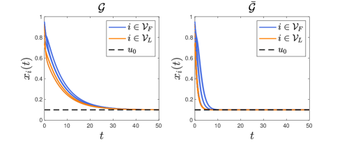
Figure 5: The agents trajectories of CLFN (2) on the network $\mathcal{G}_{7}$ in Figure 3 and its FSN network $\bar{\mathcal{G}}_{7}^{\text{CLFN}}$ in Figure 4 (left), respectively. The trajectories of leaders and external input $u_{0}$ are highlighted by yellow solid lines and black dashed lines, respectively.

Let

$$g_{ij}(t)=\frac{\|\dot{x}_{i}(t)\|}{\|\dot{x}_{j}(t)\|},i,j\in\mathcal{V}.$$ (59)

Figure 6 shows that the trajectory of $g_{ij}(t)$ in (59) for CLFN (2) where $i=3$ and $j\in\mathcal{N}_{3}=\left\{2,5,6\right\}$, asymptotically converges to $\boldsymbol{v}_{1}(L_{B})_{ij}$, as predicted by Theorem 3.

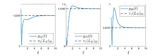
Figure 6: The $g_{ij}(t)$ in (59) for CLFN (2) where $i=3$ and $j\in\mathcal{N}_{i}=\left\{2,5,6\right\}$.

7.2 Discrete-time Case

Consider the DLFN (24) on $\mathcal{G}_{7}$ in Figure 3 with the leader set $\mathcal{V}_{\text{L}}=\left\{1,5\right\}$, where

$$P=\left(\begin{array}[]{ccccccc}\frac{1}{5}&\frac{1}{5}&0&\frac{1}{5}&0&\frac{1}{5}&0\\ \frac{1}{2}&\frac{1}{2}&0&0&0&0&0\\ 0&\frac{1}{4}&\frac{1}{4}&0&\frac{1}{4}&\frac{1}{4}&0\\ 0&0&\frac{1}{2}&\frac{1}{2}&0&0&0\\ 0&0&\frac{1}{4}&0&\frac{1}{4}&\frac{1}{4}&0\\ 0&0&0&\frac{1}{3}&0&\frac{1}{3}&\frac{1}{3}\\ \frac{1}{2}&0&0&0&0&0&\frac{1}{2}\end{array}\right);$$

computing $\boldsymbol{v}_{n}(P)$ yields,

$$\boldsymbol{v}_{n}(P) = (0.3305,\thinspace 0.3675,\thinspace 0.3923,\thinspace 0.4363,$$

$$0.2956,\thinspace 0.4348,\thinspace 0.3675)^{\top}.$$

Similar to the continuous-time case, we choose $u_{1}=u_{2}=u_{0}=0.1$. The agents’ trajectories of DLFN (24) on the network $\mathcal{G}_{7}$ in Figure 3 and its FSN network $\bar{\mathcal{G}}_{7}^{\text{DLFN}}$ in Figure 4 (right) are shown in Figure 7. One notes that the convergence rate on the corresponding FSN network has been dramatically enhanced. Figure 8 shows that the trajectory of $g_{ij}(k)$ in (58) for DLFN (24) where $i=3$ and $j\in\mathcal{N}_{3}=\left\{2,5,6\right\}$, asymptotically converges to $\boldsymbol{v}_{n}(P)_{ij}$, as predicted by Theorem 6.

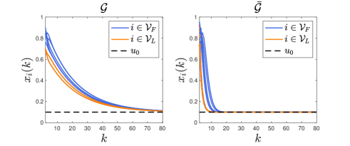
Figure 7: The agents trajectories of DLFN (24) on the network $\mathcal{G}_{7}$ in Figure 3 and its FSN network $\bar{\mathcal{G}}_{7}^{\text{DLFN}}$ in Figure 4 (right), respectively. The trajectories of leaders and external input $u_{0}$ are highlighted by yellow solid lines and black dashed lines, respectively.

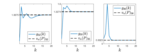
Figure 8: The $g_{ij}(k)$ in (58) for DLFN (24) where $i=3$ and $j\in\mathcal{N}_{i}=\left\{2,5,6\right\}$.

An intriguing observation is that the FSN networks of the strongly connected directed network $\mathcal{G}_{7}$ in Figure 3 constructed by using $\boldsymbol{v}_{1}(L_{B})$ and $\boldsymbol{v}_{n}(P)$, respectively, are identifcal; see Figures 4.

7.3 Adaptivity to Leader Switching

We now consider the scenario where the leader set switches over the time interval $t=[0,150]$, that is,

$$\mathcal{V}_{\text{L}}=\begin{cases}\left\{1\right\},&t=[0,50],\\ \left\{6\right\},&t=[50,100],\\ \left\{2,7\right\},&t=[100,150].\end{cases}$$

Consider the CLFN (2) on $\mathcal{G}_{7}$ in Figure 3 with leader set for each time interval defined above. The external input is such that $u_{1}=0.1$ for $t=[0,50]$, $u_{1}=0.9$ for $t=[50,100]$ and $u_{1}=u_{2}=0.1$ for $t=[100,150]$. According to Figure 9, the convergence rate has been dramatically enhanced on each time interval where the leader agent is fixed. The FSN networks of $\mathcal{G}_{7}$ in Figure 3 with $\mathcal{V}_{\text{F}}=\left\{1\right\}$, $\mathcal{V}_{\text{F}}=\left\{6\right\}$ and $\mathcal{V}_{\text{F}}=\left\{2,7\right\}$ are shown in Figure 10 and Figure 11, respectively. One can see that the eigenvector $\boldsymbol{v}_{1}(L_{B})$ is shaped by the selection of leaders, explaining the origin of structural adaptivity of diffusively coupled, directed networks. Parallel properties also hold for DLFNs, omitted here for brevity.

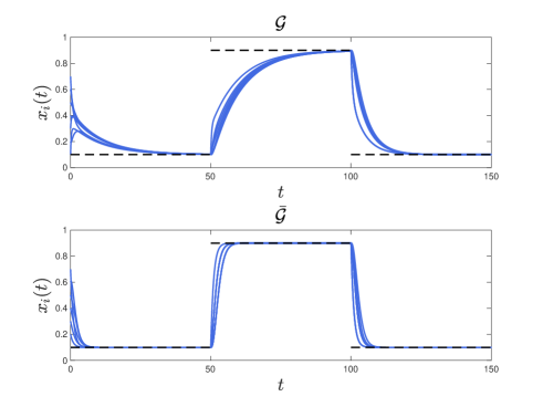
Figure 9: The agents’ trajectories along with the leader switching of original network $\mathcal{G}$ and the corresponding FSN network $\bar{\mathcal{G}}$. The black dashed lines represent pair-wise constant external inputs.

Figure 10: The FSN network of $\mathcal{G}_{7}$ in Figure 3 with $\mathcal{V}_{\text{F}}=\left\{1\right\}$. The incoming edges of nodes with in-degree more than $2$ are highlighted by dashed lines (left). The FSN network of $\mathcal{G}_{7}$ in Figure 3 with $\mathcal{V}_{\text{F}}=\left\{6\right\}$. The incoming edges of nodes with in-degree more than $2$ are highlighted by dashed lines (right).

Figure 11: The FSN network of $\mathcal{G}_{7}$ in Figure 3 with $\mathcal{V}_{\text{F}}=\left\{2,7\right\}$. The incoming edges of nodes with in-degree more than $2$ are highlighted by dashed lines.

7.4 Distributed Construction of Directed Spanning Tree

We continue to consider distributed construction of the directed spanning tree by examining the nodes with in-degree more than $2$ in FSN networks in §7.3. According to Theorem 7, these nodes can remain incident with only one incoming edge in the directed spanning tree construction.

Figure 12: A directed spanning tree of $\mathcal{G}_{7}$ in Figure 3 with $\mathcal{V}_{\text{F}}=\left\{1\right\}$, where edge $(5,3)$ removed from the FSN network in Figure 10 (left) and a directed spanning tree of $\mathcal{G}_{7}$ in Figure 3 with $\mathcal{V}_{\text{F}}=\left\{6\right\}$, where edge $(3,6)$ is removed from the FSN network in Figure 10 (right).

Specifically, for the case that $\mathcal{V}_{\text{F}}=\left\{1\right\}$, agent $5$ has in-degree $2$. As such, one can remove one of the edges in $\left\{(5,3),(5,6)\right\}$; see Figure 12 (left); for the case that $\mathcal{V}_{\text{F}}=\left\{6\right\}$, agent $3$ has in-degree $2$. Then one can remove one of the edges in $\left\{(3,5),(3,6)\right\}$; see Figure 12 (right).

8 Concluding Remarks

This paper addressed structural adaptivity problem of directed multi-agent networks that are subject to diffusion performance and exogenous influence. A distributed data-driven neighbor selection framework was developed to adjust the network connectivity adaptively to enhance the propagation of exogenous influence over the network. Both continuous-time and discrete-time directed networks were discussed. In this direction, reachability properties encoded in the eigenvectors of perturbed variants of the graph Laplacian and the SIA matrix of the underlying directed networks were extensively used. An eigenvector-based rule for neighbor selection was proposed to derive a reduced network with better convergence performance. Quantitative connections between eigenvectors of the perturbed graph Laplacian and SIA matrix and relative rate of change in agent state were then established. This connection was then utilized to develop a local data-driven inference protocol to reduce the number neighbors for each agent. This neighbor selection framework was further extended for distributed construction of directed spanning trees in directed networks.

The main results in this paper provide novel insights into the data-driven control of multi-agent networks. Although this paper mainly discussed the leader-follower consensus problem where the external input is homogeneous, analogous results can be obtained for the case of heterogeneous external input which has been extensively examined in the context of containment control of multi-agent systems [12, 26, 31]. Future works include examining networked systems with general agent dynamics and time-varying network structures.

References

- Ahmadian et al. [2018] Sajad Ahmadian, Majid Meghdadi, and Mohsen Afsharchi. A social recommendation method based on an adaptive neighbor selection mechanism. Information Processing & Management, 54(4):707–725, 2018.
- Alanwar et al. [2021] Amr Alanwar, Anne Koch, Frank Allgöwer, and Karl Henrik Johansson. Data-driven reachability analysis from noisy data. arXiv preprint arXiv:2105.07229, 2021.
- Altafini [2013] Claudio Altafini. Consensus problems on networks with antagonistic interactions. IEEE Transactions on Automatic Control, 58(4):935–946, 2013.
- Anderson et al. [2010] Brian DO Anderson, Changbin Yu, and A Stephen Morse. Convergence of periodic gossiping algorithms. In Perspectives in Mathematical System Theory, Control, and Signal Processing, pages 127–138. Springer, 2010.
- Åström and Wittenmark [2013] Karl J Åström and Björn Wittenmark. Adaptive control. Courier Corporation, 2013.
- Ballerini et al. [2008] Michele Ballerini, Nicola Cabibbo, Raphael Candelier, Andrea Cavagna, Evaristo Cisbani, Irene Giardina, Vivien Lecomte, Alberto Orlandi, Giorgio Parisi, Andrea Procaccini, et al. Interaction ruling animal collective behavior depends on topological rather than metric distance: Evidence from a field study. Proceedings of the National Academy of Sciences, 105(4):1232–1237, 2008.
- Barooah and Hespanha [2007] Prabib Barooah and Joao P Hespanha. Estimation on graphs from relative measurements. IEEE Control Systems Magazine, 27(4):57–74, 2007.
- Biyikoglu et al. [2007] Türker Biyikoglu, Josef Leydold, and Peter F Stadler. Laplacian eigenvectors of graphs: Perron-Frobenius and Faber-Krahn type theorems. Springer, 2007.
- Bliss and Govindasamy [2013] Daniel W Bliss and Siddhartan Govindasamy. Adaptive wireless communications. Cambridge University Press, 2013.
- Blondel et al. [2005] Vincent Blondel, Julien M Hendrickx, Alex Olshevsky, J Tsitsiklis, et al. Convergence in multiagent coordination, consensus, and flocking. In IEEE Conference on Decision and Control, volume 44, page 2996. IEEE; 1998, 2005.
- Cao et al. [2008] Ming Cao, A Stephen Morse, and Brian DO Anderson. Reaching a consensus in a dynamically changing environment: A graphical approach. SIAM Journal on Control and Optimization, 47(2):575–600, 2008.
- Cao et al. [2012] Yongcan Cao, Wei Ren, and Magnus Egerstedt. Distributed containment control with multiple stationary or dynamic leaders in fixed and switching directed networks. Automatica, 48(8):1586–1597, 2012.
- Chapman and Mesbahi [2013] Airlie Chapman and Mehran Mesbahi. Semi-autonomous consensus: Network measures and adaptive trees. IEEE Transactions on Automatic Control, 58(1):19–31, 2013.
- Chiuso and Pillonetto [2012] Alessandro Chiuso and Gianluigi Pillonetto. A bayesian approach to sparse dynamic network identification. Automatica, 48(8):1553–1565, 2012.
- Chung et al. [2018] Soon-Jo Chung, Aditya Avinash Paranjape, Philip Dames, Shaojie Shen, and Vijay Kumar. A survey on aerial swarm robotics. IEEE Transactions on Robotics, 34(4):837–855, 2018.
- Clark et al. [2018] Andrew Clark, Qiqiang Hou, Linda Bushnell, and Radha Poovendran. Maximizing the smallest eigenvalue of a symmetric matrix: A submodular optimization approach. Automatica, 95:446–454, 2018.
- Dibaji et al. [2019] Seyed Mehran Dibaji, Mohammad Pirani, David Bezalel Flamholz, Anuradha M Annaswamy, Karl Henrik Johansson, and Aranya Chakrabortty. A systems and control perspective of CPS security. Annual Reviews in Control, 47:394–411, 2019.
- Dörfler et al. [2013] Florian Dörfler, Michael Chertkov, and Francesco Bullo. Synchronization in complex oscillator networks and smart grids. Proceedings of the National Academy of Sciences, 110(6):2005–2010, 2013.
- Duchi et al. [2012] John C Duchi, Alekh Agarwal, and Martin J Wainwright. Dual averaging for distributed optimization: convergence analysis and network scaling. IEEE Transactions on Automatic Control, 57(3):592–606, 2012.
- Fiedler [1975] Miroslav Fiedler. A property of eigenvectors of nonnegative symmetric matrices and its application to graph theory. Czechoslovak Mathematical Journal, 25(4):619–633, 1975.
- Gardner et al. [2003] Timothy S Gardner, Diego Di Bernardo, David Lorenz, and James J Collins. Inferring genetic networks and identifying compound mode of action via expression profiling. Science, 301(5629):102–105, 2003.
- Ghaderi and Srikant [2014] Javad Ghaderi and R Srikant. Opinion dynamics in social networks with stubborn agents: Equilibrium and convergence rate. Automatica, 50(12):3209–3215, 2014.
- Horn and Johnson [2012] Roger A Horn and Charles R Johnson. Matrix Analysis. Cambridge University Press, 2012.
- Jadbabaie et al. [2003] A. Jadbabaie, Jie Lin, and A.S. Morse. Coordination of groups of mobile autonomous agents using nearest neighbor rules. IEEE Transactions on Automatic Control, 48(6):988–1001, 2003.
- Jadbabaie et al. [2018] Ali Jadbabaie, Alexander Olshevsky, George J Pappas, and Vasileios Tzoumas. Minimal reachability is hard to approximate. IEEE Transactions on Automatic Control, 64(2):783–789, 2018.
- Ji et al. [2008] Meng Ji, Giancarlo Ferrari-Trecate, Magnus Egerstedt, and Annalisa Buffa. Containment control in mobile networks. IEEE Transactions on Automatic Control, 53(8):1972–1975, 2008.
- Kia et al. [2019] Solmaz S Kia, Bryan Van Scoy, Jorge Cortes, Randy A Freeman, Kevin M Lynch, and Sonia Martinez. Tutorial on dynamic average consensus: The problem, its applications, and the algorithms. IEEE Control Systems Magazine, 39(3):40–72, 2019.
- Kim and Mesbahi [2006] Yoonsoo Kim and Mehran Mesbahi. On maximizing the second smallest eigenvalue of a state-dependent graph Laplacian. IEEE transactions on Automatic Control, 51(1):116–120, 2006.
- Leonard and Fiorelli [2001] Naomi Ehrich Leonard and Edward Fiorelli. Virtual leaders, artificial potentials and coordinated control of groups. In Proceedings of the 40th IEEE Conference on Decision and Control, volume 3, pages 2968–2973. IEEE, 2001.
- Lin et al. [2005] Zhiyun Lin, Bruce Francis, and Manfredi Maggiore. Necessary and sufficient graphical conditions for formation control of unicycles. IEEE Transactions on Automatic Control, 50(1):121–127, 2005.
- Liu et al. [2012] Huiyang Liu, Guangming Xie, and Long Wang. Necessary and sufficient conditions for containment control of networked multi-agent systems. Automatica, 48(7):1415–1422, 2012.
- Lu and Zhu [2019] Yang Lu and Minghui Zhu. A control-theoretic perspective on cyber-physical privacy: Where data privacy meets dynamic systems. Annual Reviews in Control, 47:423–440, 2019.
- Merris [1998] Russell Merris. Laplacian graph eigenvectors. Linear Algebra and Its Applications, 278(1):221–236, 1998.
- Mesbahi and Egerstedt [2010] Mehran Mesbahi and Magnus Egerstedt. Graph Theoretic Methods in Multiagent Networks. Princeton University Press, 2010.
- Nabi-Abdolyousefi and Mesbahi [2012] Marzieh Nabi-Abdolyousefi and Mehran Mesbahi. Network identification via node knockout. IEEE Transactions on Automatic Control, 57(12):3214–3219, 2012.
- Nedic [2020] Angelia Nedic. Distributed gradient methods for convex machine learning problems in networks: Distributed optimization. IEEE Signal Processing Magazine, 37(3):92–101, 2020.
- Nedich et al. [2015] Angelia Nedich et al. Convergence rate of distributed averaging dynamics and optimization in networks. Foundations and Trends® in Systems and Control, 2(1):1–100, 2015.
- Olfati-Saber and Murray [2004] Reza Olfati-Saber and Richard M Murray. Consensus problems in networks of agents with switching topology and time-delays. IEEE Transactions on Automatic Control, 49(9):1520–1533, 2004.
- Olfati-Saber et al. [2007] Reza Olfati-Saber, Alex Fax, and Richard M Murray. Consensus and cooperation in networked multi-agent systems. Proceedings of the IEEE, 95(1):215–233, 2007.
- Olshevsky and Tsitsiklis [2009] Alex Olshevsky and John N Tsitsiklis. Convergence speed in distributed consensus and averaging. SIAM Journal on Control and Optimization, 48(1):33–55, 2009.
- Pirani and Sundaram [2016] Mohammad Pirani and Shreyas Sundaram. On the smallest eigenvalue of grounded laplacian matrices. IEEE Transactions on Automatic Control, 61(2):509–514, 2016.
- Proskurnikov and Tempo [2017] Anton V Proskurnikov and Roberto Tempo. A tutorial on modeling and analysis of dynamic social networks. part i. Annual Reviews in Control, 43:65–79, 2017.
- Proskurnikov and Tempo [2018] Anton V Proskurnikov and Roberto Tempo. A tutorial on modeling and analysis of dynamic social networks. part ii. Annual Reviews in Control, 2018.
- Ren et al. [2005] Wei Ren, Randal W Beard, et al. Consensus seeking in multiagent systems under dynamically changing interaction topologies. IEEE Transactions on Automatic Control, 50(5):655–661, 2005.
- Seneta [2006] Eugene Seneta. Non-negative Matrices and Markov Chains. Springer, 2006.
- Shahrampour and Preciado [2014] Shahin Shahrampour and Victor M Preciado. Topology identification of directed dynamical networks via power spectral analysis. IEEE Transactions on Automatic Control, 60(8):2260–2265, 2014.
- Shao and Mesbahi [2014] Haibin Shao and Mehran Mesbahi. Degree of relative influence for consensus-type networks. In American Control Conference, pages 2676–2681, 2014.
- Shao et al. [2017] Haibin Shao, Mehran Mesbahi, Dewei Li, and Yugeng Xi. Inferring centrality from network snapshots. Scientific reports, 7:40642, 2017.
- Shao et al. [2019] Haibin Shao, Lulu Pan, Mehran Mesbahi, Yugeng Xi, and Dewei Li. Relative tempo of distributed averaging on networks. Automatica, 105:159–166, 2019.
- Shao et al. [2021] Haibin Shao, Lulu Pan, Mehran Mesbahi, Yugeng Xi, and Dewei Li. Distributed neighbor selection in multi-agent networks. arXiv preprint arXiv:2107.12022, 2021.
- Song et al. [2020] Yue Song, David J Hill, Tao Liu, et al. Network-based analysis of rotor angle stability of power systems. Foundations and Trends® in Electric Energy Systems, 4(3):222–345, 2020.
- Vicsek and Zafeiris [2012] Tamás Vicsek and Anna Zafeiris. Collective motion. Physics Reports, 517(3):71–140, 2012.
- Vicsek et al. [1995] Tamás Vicsek, András Czirók, Eshel Ben-Jacob, Inon Cohen, and Ofer Shochet. Novel type of phase transition in a system of self-driven particles. Physical Review Letters, 75(6):1226, 1995.
- Wada et al. [1990] Ben K Wada, James L Fanson, and Edward F Crawley. Adaptive structures. Journal of Intelligent Material Systems and Structures, 1(2):157–174, 1990.
- Wagg et al. [2008] David Wagg, Ian Bond, Paul Weaver, and Michael Friswell. Adaptive structures: engineering applications. John Wiley & Sons, 2008.
- Xia and Cao [2017] Weiguo Xia and Ming Cao. Analysis and applications of spectral properties of grounded laplacian matrices for directed networks. Automatica, 80:10–16, 2017.
- Zafeiris and Vicsek [2017] Anna Zafeiris and Tamás Vicsek. Why We Live in Hierarchies?: A Quantitative Treatise. Springer, 2017.