Maximum $k$-Biplex Search on Bipartite Graphs: A Symmetric-BK Branching Approach

Abstract.

Enumerating maximal $k$-biplexes (MBPs) of a bipartite graph has been used for applications such as fraud detection. Nevertheless, there usually exists an exponential number of MBPs, which brings up two issues when enumerating MBPs, namely the effectiveness issue (many MBPs are of low values) and the efficiency issue (enumerating all MBPs is not affordable on large graphs). Existing proposals of tackling this problem impose constraints on the number of vertices of each MBP to be enumerated, yet they are still not sufficient (e.g., they require to specify the constraints, which is often not user-friendly, and cannot control the number of MBPs to be enumerated directly). Therefore, in this paper, we study the problem of finding $K$ MBPs with the most edges called MaxBPs, where $K$ is a positive integral user parameter. The new proposal well avoids the drawbacks of existing proposals (i.e., the number of MBPs to be enumerated is directly controlled and the MBPs to be enumerated tend to have high values since they have more edges than the majority of MBPs). We formally prove the NP-hardness of the problem. We then design two branch-and-bound algorithms, among which, the better one called FastBB improves the worst-case time complexity to $O^{*}(\gamma_{k}^{n})$, where $O^{*}$ suppresses the polynomials, $\gamma_{k}$ is a real number that relies on $k$ and is strictly smaller than 2, and $n$ is the number of vertices in the graph. For example, for $k=1$, $\gamma_{k}$ is equal to $1.754$. We further introduce three techniques for boosting the performance of the branch-and-bound algorithms, among which, the best one called PBIE can further improve the time complexity to $O^{*}(\gamma_{k}^{d^{3}})$ for large sparse graphs, where $d$ is the maximum degree of the graph (note that $d<<n$ for sparse graphs). We conduct extensive experiments on both real and synthetic datasets, and the results show that our algorithm is up to four orders of magnitude faster than all baselines and finding MaxBPs works better than finding all MBPs for a fraud detection application.

1. introduction

Bipartite graph is an important type of data structure where vertices are divided into two disjoint sets at two sides and each edge connects a vertex at one side and another at the other side. Bipartite graphs have been widely used for modeling the interactions between two types of entities in many real applications, with the entities being vertices and the interactions being edges. Some examples include commenting interactions between users and articles in social media (Zhang and Ghorbani, 2020), purchasing interactions between customers and products in E-commerce (Wang et al., 2006), visiting interactions between users and websites in web applications (Beutel et al., 2013), etc.

A bipartite subgraph is called a $k$-biplex if each vertex at one side disconnects at most $k$ vertices at the other side, where $k$ is often a small positive integer (Sim et al., 2009; Yu et al., 2021, 2022). $k$-biplex has been used to capture dense/cohesive subgraphs in a given bipartite graph for solving practical problems such as anomaly detection (Gangireddy et al., 2020; Yu and Long, 2021), online recommendation (Poernomo and Gopalkrishnan, 2009; Günnemann et al., 2011) and community search (Hao et al., 2020; Wang et al., 2021). For example, in e-commerce platforms, some agents are paid to promote the ranks of certain products by coordinating a group of fake users to post fake comments. The subgraphs induced by these fake users and the products they promote would be dense and likely to be $k$-biplexes (Gangireddy et al., 2020).

Motivations. There are a few studies on the problem of enumerating maximal $k$-biplexes (MBPs) (Sim et al., 2009; Yu et al., 2021, 2022). Nevertheless, there usually exist an exponential number of MBPs, which brings two issues of enumerating all MBPs. First, not all MBPs carry essential information (e.g., those MBPs with few vertices are often deemed not interesting (Sim et al., 2009)). Second, the process of enumerating all MBPs is costly (e.g., according to existing studies (Yu et al., 2021), enumerating all MBPs on large graphs is not affordable). To mitigate these issues, existing studies (Yu et al., 2022) impose some constraints on the number of vertices at each of the two sides of a MBP to be enumerated, e.g., they enumerate only MBPs with at least a certain number vertices at each side (which we call large MBPs). While this strategy makes it possible to control the number of MBPs to be enumerated, it achieves the goal only in an indirect way and introduces an additional issue of requiring to set proper thresholds of the number of vertices. In cases where users have no prior knowledge about the thresholds, they would find it not user-friendly. They can try different thresholds, but then the enumeration processes would run multiple times and bring up the time costs.

Motivated by these issues, in this paper, we study the problem of finding $K$ MBPs with the most edges among large MBPs, where $K$ is an integral parameter. We call each of these MBPs a maximum $k$-biplex (MaxBP). Compared with existing studies on $k$-biplexes, the problem of finding MaxBPs enjoys three advantages. First, each MaxBP to be found has more edges than those that are not returned, and thus the found MBP is of more significance. In our experiments, we verify this via a case study, which shows that a method based on MaxBPs provides F1 score up to 0.99 for a fraud detection task. Second, it provides a direct control on the number of MBPs to be found without the need of making multiple trials of enumeration. Third, compared with alternative proposals, e.g., finding the first $K$ MBPs (as existing studies (Yu et al., 2022) do) or finding $K$ MBPs with the most vertices, our solution to the problem of finding MaxBPs would return MBPs that are more balanced, which are deemed to be superior over imbalanced structures (Lyu et al., 2020).

Baseline Methods. Given the fact that MaxBPs are the MBPs with the most edges, we can adapt the existing algorithms of enumerating large MBPs, namely iMB (Yu et al., 2021) and iTraversal (Yu et al., 2022), to find the MaxBPs and yield the following two baseline methods. The first one called iMBadp adapts iMB (Yu et al., 2021) (a branch-and-bound algorithm) by incorporating additional pruning techniques which prune those branches that cannot hold any MBP with more edges than the $K$ MaxBPs found so far. The second baseline called iTradp simply runs iTraversal (Yu et al., 2022) (a reverse search based algorithm) and returns $K$ MaxBPs since iTraversal cannot be equipped with additional pruning techniques easily. Nevertheless, iMBadp has its efficiency highly rely on the pruning techniques and iTradp needs to explore all large MBPs, which is time-consuming. Both of them have the worst-case time complexity of $O^{*}(2^{n})$, where $n$ is the number of vertices in the given bipartite graph and $O^{*}$ suppresses polynomials. Furthermore, we can adapt those existing algorithms of enumerating large maximal $k$-plexes, which are counterparts of MBPs on general graphs. Here, a $k$-plex is a subgraph with each vertex disconnecting at most $k$ vertices in the subgraph. Therefore, the third baseline method called FPadp adapts FaPlexen (Zhou et al., 2020) (the algorithm for enumerating large maximal $k$-plexes with the number of vertices at least a threshold) with some additional pruning techniques that are tailored for MBPs. Still, FPadp is inferior to the new algorithms we will introduce in this paper both theoretically and empirically.

New Methods. We first introduce a branch-and-bound algorithm called BasicBB, which is based on a conventional and widely-used branching strategy that we call Bron-Kerbosch (BK) branching (Bron and Kerbosch, 1973). The BK branching recursively partitions the search space (i.e., the set of all possible MBPs) to multiple sub-spaces via branching. BasicBB has the worst-case time complexity $O(n\cdot d\cdot 2^{n})$ (i.e., $O^{*}(2^{n})$), where $d$ is the maximum degree of the graph. This time complexity is the same as those of the baseline methods. We then introduce a new branching strategy called Symmetric-BK (Sym-BK) branching, which is symmetric to the BK branching but better suits our problem of finding MaxBPs. We further present our method for determining an ordering of vertices, which is critical for Sym-BK branching. We finally introduce a new branch-and-bound algorithm called FastBB, which is based on the Sym-BK branching. FastBB has its worst-case time complexity $O(n\cdot d\cdot\gamma_{k}^{n})$ (i.e., $O^{*}(\gamma_{k}^{n})$), where $\gamma_{k}$ is strictly smaller than 2 and depends on the setting of $k$. For example, when $k=1$, $\gamma_{k}$ is $1.754$. This is a remarkable theoretical improvement over the prior solutions given that many existing algorithms of enumerating subgraphs are based on BK branching and have the worst-case time complexity of $O^{*}(2^{n})$ (Sim et al., 2009; Yu et al., 2021; Wang et al., 2017).

In addition, we adapt two existing techniques for boosting the efficiency and scalability of the branch-and-bound (BB) algorithms including BasicBB and FastBB. They share the idea of constructing multiple problem instances of finding MaxBPs each on a smaller subgraph. Specifically, the first technique, called progressive bounding (PB), is adapted from an existing study of finding the biclique with the most edges (Lyu et al., 2020). The second technique, called inclusion-exclusion (IE), is adapted from the decomposition technique, which has been widely used for enumerating and finding subgraph structures (Wang et al., 2022; Chen et al., 2021; Conte et al., 2018). PB improves the practical performance of a BB algorithm only while IE improves both the theoretical time complexity (for certain sparse graphs) and the practical performance. We then present PBIE, which combines PB and IE naturally. PBIE enjoys the benefits of both PB and IE. We note that all these techniques are orthogonal to the BB algorithms, i.e., any of these techniques, namely PB, IE, and PBIE, can be used to boost the efficiency and/or scalability of BasicBB and FastBB. To the best of our knowledge, this is first time that PB and IE are combined naturally.

Contributions. Our major contributions are summarized below.

• We study the problem of finding MaxBPs, and formally prove the NP-hardness of the problem.

• We propose an efficient branch-and-bound algorithm, called FastBB, which is based on a novel Sym-BK branching strategy. In particular, FastBB achieves the state-of-the-art worst-case time complexity $O(n\cdot d\cdot\gamma_{k}^{n})$ with $\gamma_{k}<2$.

• We further introduce a combined framework, called PBIE, to further boost the performance of FastBB. PBIE combines two adapted frameworks, namely the progressive bounding framework PB and the inclusion-exclusion based framework IE. When PBIE is used with FastBB, the worst-time time complexity becomes $O(d^{4}\cdot\gamma_{k}^{d^{3}})$. Note that this is better than that of FastBB on certain graphs (e.g., those sparse graphs with $d<<n$).

• We conduct extensive experiments using both real and synthetic datasets, and the results show that (1) the proposed algorithms are up to four orders of magnitude faster than all baselines and (2) finding MaxBPs work better in a fraud detection task than enumerating MBPs.

Roadmap. The rest of this paper is organized below. Section 2 defines the problem and shows its NP-hardness. Section 3 presents the branch-and-bound algorithms BasicBB and FastBB. Section 4 presents the frameworks PB, IE and PBIE. We conduct extensive experiments in Section 5. Section 6 reviews the related work and Section 7 concludes the paper.

2. problem definition

Let $G=(L\cup R,E)$ be an undirected and unweighted bipartite graph, where $L$ and $R$ are two disjoint vertex sets and $E$ is an edge set. For the graph $G$, we use $V(G)$, $L(G)$, $R(G)$, and $E(G)$ to denote its set of vertices, left side, right side and set of edges, respectively, i.e., $V(G)=L\cup R$, $L(G)=L$, $R(G)=R$, and $E(G)=E$. Given $X\subseteq L$ and $Y\subseteq R$, we use $G[X\cup Y]$ to denote the induced (bipartite) graph of $G$, i.e., $G[X\cup Y]$ includes the set of vertices $X\cup Y$ and the set of edges between $X$ and $Y$. All subgraphs considered in this paper are induced subgraphs. We use $H$ or $(X,Y)$ as a shorthand of $H=G[X\cup Y]$.

Given $v\in L$, we use $\Gamma(v,R)$ (resp. $\overline{\Gamma}(v,R)$) to denote the set of neighbours (resp. non-neighbours) of $v$ in $R$, i.e., $\Gamma(v,R)=\{u\mid(v,u)\in E\ \text{and}\ u\in R\}$ (resp. $\overline{\Gamma}(v,R)=\{u\mid(v,u)\notin E\ \text{and}\ u\in R\}$). We define $\delta(v,R)=|\Gamma(v,R)|$ and $\overline{\delta}(v,R)=|\overline{\Gamma}(v,R)|$. We use $d$ to denote the maximum degree of vertex in $G$. We have symmetric definitions for each vertex $u\in R$. Next, we review the definition of $k$-biplex (Yu et al., 2021).

Definition 0 ($k$-biplex (Yu et al., 2021)).

Given a graph $G=(L,R,E)$, a positive integer $k$, $X\subseteq L$ and $Y\subseteq R$, a subgraph $G[X\cup Y]$ is said to be a $k$-biplex if $\overline{\delta}(v,Y)\leq k$, $\forall v\in X$ and $\overline{\delta}(u,X)\leq k$, $\forall u\in Y$.

A $k$-biplex $H$ is said to be maximal if there is no other $k$-biplex $H^{\prime}$ containing $H$, i.e., $V(H)\subseteq V(H^{\prime})$. Large real graphs usually involve numerous maximal $k$-biplexes and most of them highly overlap. In this paper, we aim to find $K$ maximal $k$-biplexes with the most edges, where $K$ is a positive integral user-parameter. In addition, we consider two size constraints $\theta_{L}$ and $\theta_{R}$ on each maximal $k$-biplex $H$ to be found, namely $|L(H)|\geq\theta_{L}$ and $|R(H)|\geq\theta_{R}$. These constraints would help to filter out some skewed maximal $k$-biplexes, i.e., the number of vertices at one side is extremely larger than that at the other side. To guarantee that all found maximal $k$-biplexes are connected, we further require $\theta_{L}\geq 2k+1$ and $\theta_{R}\geq 2k+1$ based on the following lemma.

Lemma 0.

A $k$-biplex $H$ is connected if $|L(H)|\geq 2k+1$ and $|R(H)|\geq 2k+1$.

Proof.

This can be proved by contradiction. Suppose $H$ is not connected and is partitioned into two connected components, namely $H_{1}$ and $H_{2}$. We derive the contradiction by showing that $H$ is not a $k$-biplex: for a vertex $v_{1}$ in $L(H_{1})$, it disconnects more than $k$ vertices, i.e., $\overline{\delta}(v_{1},R(H))\geq|R(H_{2})|\geq k+1$. Specifically, we derive $\overline{\delta}(v_{1},R(H))\geq|R(H_{2})|$ since $v_{1}$ from $H_{1}$ disconnects all vertices in $H_{2}$ based on the assumption, and we derive $|R(H_{2})|\geq k+1$ by (1) for a vertex $v_{2}$ in $L_{2}$, $|R(H_{2})|\geq\delta(v_{2},R(H))$ since all neighbours of $v_{2}$ within $H$ reside in $R(H_{2})$ based on the assumption and (2) $\delta(v_{2},R(H))\geq R(H)-k\geq 2k+1-k\geq k+1$ since $v_{2}$ disconnects at most $k$ vertices ($H$ is a $k$-biplex) and $R(H)\geq 2k+1$. ∎

We formalize the problem studied in this paper as follows.

Problem 1 (Maximum $k$-biplex Search).

Given a bipartite graph $G=(L\cup R,E)$, four positive integers $K>0$, $k>0$, $\theta_{L}\geq 2k+1$ and $\theta_{R}\geq 2k+1$, the maximum $k$-biplex search problem aims to find $K$ maximal $k$-biplexes such that each found maximal $k$-biplex $H$ satisfies that $|L(H)|\geq\theta_{L}$, $|R(H)|\geq\theta_{R}$ and $|E(H)|$ is larger than $|E(H^{\prime})|$ for any other maximal $k$-biplex $H^{\prime}$ that is not returned.

In this paper, we use MBP and MaxBP as a shorthand of a maximal $k$-biplex and one of the $K$ maximal $k$-biplexes with the most edges, respectively.

NP-hardness. The maximum $k$-biplex search problem is NP-hard, which we present in the following lemma (with its proof provided in Section 8 ).

Lemma 0.

The maximum $k$-biplex search problem is NP-hard.

Remarks. In the following sections (Section 3 and Section 4), we focus on the setting of $K=1$ (i.e., the problem becomes to find a MBP with the maximum number of edges) when presenting the algorithms for ease of presentation. We note that these algorithms can be naturally extended for general settings of $K$ with minimal efforts (i.e., we maintain $K$ MaxBPs instead of $1$ MaxBP found so far throughout the algorithm for pruning) and are tested in Section 5.

3. Branch-and-Bound Algorithms

We first introduce a branch-and-bound algorithm called BasicBB, which is based on a conventional and widely-used branching strategy that we call Bron-Kerbosch (BK) branching (Bron and Kerbosch, 1973), in Section 3.1. BasicBB has the worst-case time complexity $O(|V|\cdot d\cdot 2^{|V|})$. We then introduce a new branching strategy called Symmetric-BK (Sym-BK) branching, which is symmetric to the BK branching but better suits our problem of finding MaxBP, in Section 3.2. We further present our method for determining an ordering of vertices, which is critical for Sym-BK branching, in Section 3.3. We finally introduce a new branch-and-bound algorithm called FastBB, which is based on Sym-BK branching, and analyze its time complexity in Section 3.4. FastBB has its worst-case time complexity $O(|V|\cdot d\cdot\gamma_{k}^{|V|})$, where $\gamma_{k}$ is strictly smaller than 2 and depends on the setting $k$. For example, when $k=1$, $\gamma_{k}$ is $1.754$.

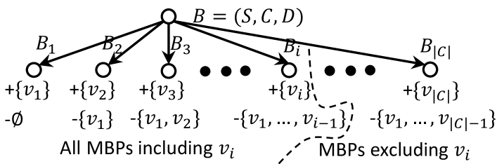
(a) BK Branching

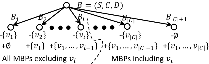
(b) Sym-BK Branching

Figure 1. Illustration of two branching strategies. Each node denotes a branch $(S,C,D)$. The notation “+” means to include a vertex by adding it $S$ and “-” means to exclude a vertex by adding it to $D$.

3.1. A BK Branching based Branch-and-Bound Algorithm: BasicBB

Our first attempt is to adapt the seminal Bron-Kerbosch (BK) algorithm (Bron and Kerbosch, 1973). It recursively partitions the search space (i.e., the set of all possible MBPs) to multiple sub-spaces via branching. Specifically, each sub-space is represented by a triplet of three sets $(S,C,D)$ as explained below.

• Partial set $S$. Set of the vertices that must be included in every MBP within the space.

• Candidate set $C$. Set of the vertices that can be included in $S$ in order to form a MBP within the space.

• Exclusion set $D$. Set of vertices that must not be included in any MBP within the space.

We further denote by $S_{L}$, $C_{L}$, and $D_{L}$ the left side of $S$, $C$, and $D$, respectively, and define $S_{R}$, $C_{R}$, and $D_{R}$ similarly for the right side.

The recursive process of the BK algorithm starts from the full search space with $S=\emptyset$, $C=V$, and $D=\emptyset$. Consider the branching step at a current branch $B=(S,C,D)$. Let $\langle v_{1},v_{2},...,v_{|C|}\rangle$ be a sequence of the vertices in $C$. The branching step would partition the space to $|C|$ sub-spaces (and correspondingly $|C|$ branches), where the $i^{th}$ branch, denoted by $B_{i}=(S_{i},C_{i},D_{i})$, includes $S$ and $v_{i}$ and excludes $v_{1},v_{2},...,v_{i-1}$. Formally, for $1\leq i\leq|C|$, we have

(1) $$S_{i}=S\cup\{v_{i}\};~{}~{}D_{i}=D\cup\{v_{1},v_{2},...,v_{i-1}\};~{}~{}C_{i}=C-\{v_{1},v_{2},...,v_{i}\}$$

For illustration, consider Figure 1(a). Note that $C_{i}$ and $D_{i}$ can be further refined by removing those vertices that cannot be included to $G[S_{i}]$ to form a $k$-biplex.

We call the above branching strategy BK branching. BK branching essentially corresponds to a recursive binary branching process. It first splits the current branch into two branches, one including $v_{1}$ (this is the branch $B_{1}$) and the other excluding $v_{1}$. Then, it further splits the latter into two branches, one including $v_{2}$ (this is the branch $B_{2}$) and the other excluding $v_{2}$. It continues the process until the last branch, which excludes $v_{1},v_{2},...,v_{|C|-1}$ and includes $v_{|C|}$ (this corresponds to the branch $B_{|C|}$), is formed. In particular, the branches $B_{1},B_{2},...,B_{i}$ cover all MBPs including $v_{i}$ and branches $B_{i+1},...,B_{|C|}$ cover those excluding $v_{i}$, as indicated by the dashed line in Figure 1(a).

We note that BK branching relies on an ordering of vertices in the candidate set $C$, i.e., $\langle v_{1},v_{2},...,v_{|C|}\rangle$, for producing branches. In this paper, we follow the existing studies (Zhang et al., 2014; Abidi et al., 2020) and use the non-decreasing vertex degree ordering (where vertices are ranked in a non-decreasing order of their degrees in $S\cup C$, i.e., $\delta(v_{i},S\cup C)\leq\delta(v_{j},S\cup C)$ for any $i<j$) since this would help with effective pruning as shown empirically. We note that normally the ordering does not affect the worst-case theoretical time complexity of the algorithm based on BK branching.

During the recursive search process, some pruning techniques can be applied. Let $B=(S,C,D)$ be a branch. First, branch $B$ can be pruned if $S$ is not a $k$-biplex since (1) each partial set in the search space corresponding to this branch is a superset of $S$ and (2) based on the hereditary property of $k$-biplex, any superset of a non-$k$-biplex is not a $k$-biplex. Second, branch $B$ can be pruned if an upper bound of the left side (resp. the right side) of a $k$-biplex in the space is smaller than $\theta_{L}$ (resp. $\theta_{R}$) based on the problem definition. Third, branch $B$ can be pruned if an upper bound of the number of edges in a $k$-biplex in the space is smaller than the largest one of a $k$-biplex known so far. Fourth, branch $B$ can be pruned if there exists a vertex in $D$ such that including this vertex to each $k$-biplex in the space would still result in a $k$-biplex. We will elaborate on these pruning rules in detail in Section 3.4. Finally, the recursive process of the BK algorithm terminates at a branch $B=(S,C,D)$ if $G[S\cup C]$ is a $k$-biplex since $G[S\cup C]$ would be the MaxBP within the space of the branch.

We call this BK algorithm, which is a branch-and-bound algorithm based on BK branching and the aforementioned four pruning techniques, BasicBB, and present its pseudo-code in Algorithm 1. Similar to many existing algorithms that are based on BK branching, the worst-case time complexity of BasicBB is $O(|V|\cdot d\cdot 2^{|V|})$ (i.e., $O^{*}(2^{|V|})$) (Yu et al., 2021; Sim et al., 2009), though its practical performance can be boosted by the the pruning techniques.

Input: A graph $G(L\cup R,E)$, $k$, $\theta_{L}$ and $\theta_{R}$

Output: The maximal $k$-biplex $H^{*}$ with the most edges

$H^{*}\leftarrow G[\emptyset]$; // Global variable

1 BasicBB-Rec$(\emptyset,L\cup R,\emptyset)$;  return $H^{*}$;

2 Procedure BasicBB-Rec$(S,C,D)$

3      

      /* Termination */

4       if $G[S\cup C]$ is $k$-biplex then

5             $H^{*}\leftarrow G[S\cup C]$ if $|E(G[S\cup C])|>|E(H^{*})|$; return;

6      

      /* Pruning */

7       if any of pruning conditions is satisfied (details in Section 3.4) then  return ;

8      

      /* BK Branching */

9       Create $|C|$ branches $B_{i}=(S_{i},C_{i},D_{i})$ based on Equation (1);

10       for each branch $B_{i}$ do

11             BasicBB-Rec$(S_{i},C_{i},D_{i})$;

12      

13

Algorithm 1 The branch-and-bound algorithm based on BK branching: BasicBB

3.2. A New Branching Strategy: Sym-BK Branching

We observe that there exists a branching strategy, which is natural and symmetric to BK branching. Specifically, consider the branching step at a current branch $B=(S,C,D)$. Let $\langle v_{1},v_{2},...,v_{|C|}\rangle$ be a sequence of the vertices in $C$. This branching step would partition the space to $(|C|+1)$ sub-spaces (and correspondingly $(|C|+1)$ branches), where the $i^{th}$ branch, denoted by $B_{i}=(S_{i},C_{i},D_{i})$, includes $S$ and $v_{1},v_{2},...,v_{i-1}$ and excludes $v_{i}$. Here, $v_{0}$ and $v_{|C|+1}$ both correspond to null. Formally, for $1\leq i\leq|C|+1$, we have

(2) $$S_{i}=S\cup\{v_{1},v_{2},...,v_{i-1}\};~{}~{}D_{i}=D\cup\{v_{i}\};~{}~{}C_{i}=C-\{v_{1},v_{2},...,v_{i}\}$$

For illustration, consider Figure 1(b). Note that $C_{i}$ and $D_{i}$ can be further refined by removing those vertices that cannot be included to $G[S_{i}]$ to form a $k$-biplex.

We call the above branching strategy symmetric-BK (Sym-BK) branching. Sym-BK branching corresponds to another recursive binary branching process, which is symmetric to that of the BK branching. Specifically, it first splits the current branch into two branches, one excluding $v_{1}$ (this is the branch $B_{1}$) and the other including $v_{1}$. Then, it further splits the latter into two branches, one excluding $v_{2}$ (this is the branch $B_{2}$) and the other including $v_{2}$. It continues the process until the last branch, which includes $v_{1},v_{2},...,v_{|C|}$ (this corresponds to the branch $B_{|C|+1}$), is formed. In particular, the branches $B_{1},B_{2},...,B_{i}$ cover all MBPs excluding $v_{i}$ and branches $B_{i+1},...,B_{|C|+1}$ cover those including $v_{i}$, as indicated by the dashed line in Figure 1(b).

Sym-BK branching vs. BK branching. They are symmetric to each other and both of them are natural branching strategies. They differ in that among two branches formed by a binary branching based on a vertex, BK branching recursively partitions the branch excluding the vertex while Sym-BK recursively partitions one including the vertex. Sym-BK branching produces one more branch than BK branching at each branching step (i.e., $|C|+1$ branches vs. $|C|$ branches), but this difference of one extra branch is negligible given that there can be many branches produced at the branching step. Compared with BK branching, Sym-BK branching has the following advantages when adopted for our problem of finding the MaxBP.

First, at each branching step, it would produce branches with bigger partial sets $S_{i}$ (note that the $i^{th}$ branch by Sym-BK branching involves $|S|+(i-1)$ vertices in the partial set while that by BK branching involves $|S|+1$ vertices). Consequently, the produced branch would have a larger chance to be pruned due to the hereditary property of $k$-biplex (if a set of vertices is not a $k$-biplex, then none of its supersets is, but not vice versa). Second, the partial set of the $j^{th}$ branch, i.e., $S_{j}$, is always a superset of that of the $i^{th}$ branch, i.e., $S_{i}$, for any $j>i$. Consequently, if $S_{i}$ is not a $k$-biplex (which means the branch $B_{i}$ can be pruned), then all branches following $B_{i}$ can be pruned (since their partial sets are supersets of $S_{i}$ and thus they are not $k$-biplexes either based on the hereditary property).

To illustrate, consider the example in Figure 2. One branching step of Sym-BK branching is shown in Figure 2(b). The fourth branch has the partial set of $S_{4}=\{u_{0},v_{0},u_{1},u_{2},u_{4}\}$, which is not a $k$-biplex. All the following branches have their partial sets as supersets of $S_{4}$, and thus they can be pruned immediately (as indicated by the shaded color in the figure).

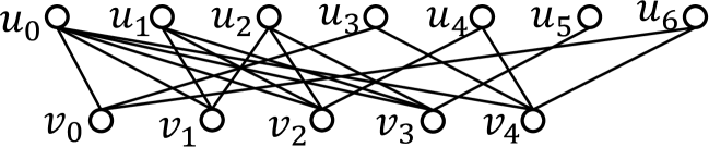
(a) Input graph used throughout the paper

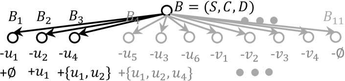
(b) Case 1 ($S=\{u_{0},v_{0}\}$, $C=\{u_{1},u_{2},u_{4},u_{5},u_{3},u_{6},v_{1},v_{2},v_{3},v_{4}\}$ and $D=\emptyset$)

(c) Case 2 ($S_{3}\!=\!\{u_{0},v_{0},u_{1},u_{2}\}$, $C_{3}\!=\!\{u_{3},v_{1},v_{2},v_{3},u_{6},v_{4}\}$ and $D_{3}\!=\!\{u_{4},u_{5}\}$)

Figure 2. Illustration of Sym-BK branching ($k=2$).

In fact, with Sym-BK branching and a carefully-designed ordering of vertices (details will be introduced in Section 3.3), our new branch-and-bound algorithm FastBB would have the worst-case time complexity of $O(|V|\cdot d\cdot\gamma_{k}^{|V|})$ with $\gamma_{k}<2$, which is strictly smaller than that of the BasicBB algorithm based on BK branching (details will be introduced in Section 3.4).

Remarks. In (Zhou et al., 2020), the authors design a branching strategy, which performs one of two branching operations at a branch depending on the situation: (1) generating two branches based on a single vertex in $C$ (i.e., one including and the other not including this vertex) and (2) generating at most $(|C|+1)$ branches based on all vertices in $C$ with pruning. We call this branching strategy hybrid branching. Our Sym-BK branching is superior over hybrid branching for our problem in two aspects. First, Sym-BK branching has a more simplified form. Second, the branch-and-bound algorithm based on Sym-BK branching has lower worst-case time complexity theoretically (details are in Section 3.4) and runs faster empirically (details are in Section 5).

3.3. Sym-BK Branching: Ordering of Vertices

The Sym-BK branching relies on an ordering of the vertices in $C$. Recall that in the branches $B_{1},B_{2},...,B_{|C|+1}$ generated by Sym-BK branching, the partial set of a branch $B_{j}$ is always a superset of that of a preceding branch $B_{i}$ ($i<j$). Therefore, our idea is to figure out a small subset $C^{\prime}$ of vertices in $C$ such that including them collectively to the partial set $S$ would violate the $k$-biplex definition. We then put these vertices before other vertices in the ordering. In this way, the branch with the partial set of $S\cup C^{\prime}$ and all the following branches can be pruned directly. We elaborate on this idea in detail next.

We notice that $G[S\cup C]$ is not a $k$-biplex since otherwise the recursion would terminate at this branch. It means that there exists at least a vertex in $S\cup C$, which has more than $k$ disconnections within $G[S\cup C]$. Without loss of generality, we assume that the vertex is from the left side and denote it by $\hat{v}\in S_{L}\cup C_{L}$. Consider the set of vertices that disconnect $\hat{v}$ in $C_{R}$, i.e., $\overline{\Gamma}(\hat{v},C_{R})$. We know that including $\overline{\Gamma}(\hat{v},C_{R})$ to $S$ collectively would violate the $k$-biplex definition. Specifically, if $\hat{v}$ is already in $S_{L}$, i.e., $\hat{v}\in S_{L}$, we can include at most $k-\overline{\delta}(\hat{v},S_{R})$ vertices from $\overline{\Gamma}(\hat{v},C_{R})$ to $S$ without violating the $k$-biplex definition; and if $\hat{v}$ is not yet in $S_{L}$, i.e., $\hat{v}\in C_{L}$, we can include $\hat{v}$ together with at most $k-\overline{\delta}(\hat{v},S_{R})$ vertices from $\overline{\Gamma}(\hat{v},C_{R})$ to $S$ without violating the $k$-biplex definition. For the simplicity of notations, we define

(3) $$a=k-\overline{\delta}(\hat{v},S_{R});~{}~{}b=\overline{\delta}(\hat{v},C_{R}).$$

Intuitively, $a$ means the greatest possible number of disconnections that $\hat{v}$ can have when including more vertices from $C$ to $S$ for forming MBPs. Note that we have $0\leq a\leq k$ (since $S$ is a $k$-biplex and thus $\overline{\delta}(\hat{v},S_{R})\leq k$) and $a<b$ (since $b-a=\overline{\delta}(\hat{v},S_{R}\cup C_{R})-k>0$). Based on $\hat{v}$, we define an ordering of the vertices in $C$.

Case 1: $\hat{v}\in S_{L}$. In this case, we define the ordering as follows.

(4) $$\langle u_{1},u_{2},...,u_{b},u_{b+1},...,u_{|C|}\rangle,$$

where $u_{1},u_{2},...,u_{b}$ are vertices from $\overline{\Gamma}(\hat{v},C_{R})$ in any order and $u_{b+1},u_{b+2},...,u_{|C|}$ are vertices from $C-\overline{\Gamma}(\hat{v},C_{R})$ in any order. Based on this ordering, the branch $B_{a+2}$ would have the partial set $S\cup\{u_{1},u_{2},...,u_{a+1}\}$, which is not a $k$-biplex (since $\hat{v}$ would have more than $k$ disconnections). Therefore, branches $B_{a+2},B_{a+3},...,B_{|C|+1}$ can be pruned and only the first $(a+1)$ branches, namely $B_{1},B_{2},...,B_{a+1}$, would be kept. To illustrate, we consider a branch with $S=\{u_{0},v_{0}\}$, $D=\emptyset$ and $C=\{u_{1},u_{2},u_{3},u_{4},u_{5},u_{6},v_{1},v_{2},v_{3},v_{4}\}$ for finding a MaxBP with $k=2$ from the input graph in Figure 2(a). Based on $v_{0}$ in $S$ that disconnects 3 vertices, i.e., $\{u_{1},u_{2},u_{4}\}$, we define the ordering $\langle u_{1},u_{2},u_{4},u_{5},u_{3},u_{6},v_{1},v_{2},v_{3},v_{4}\rangle$ for Sym-BK branching as shown in Figure 2(b). The branches $B_{4},...,B_{11}$ can be pruned since $B_{4}$ has the partial set $\{u_{0},u_{1},u_{2},u_{4},v_{0}\}$ not a $k$-biplex ($v_{0}$ has more than $k=2$ disconnections).

Case 2: $\hat{v}\in C_{L}$. In this case, we define the ordering as follows.

(5) $$\langle\hat{v},u_{1},u_{2},...,u_{b},u_{b+2},...,u_{|C|}\rangle,$$

where $u_{1},u_{2},...,u_{b}$ are vertices from $\overline{\Gamma}(\hat{v},C_{R})$ in any order and $u_{b+2},u_{b+2},...,u_{|C|}$ are vertices from $C-\overline{\Gamma}(\hat{v},C_{R})-\{\hat{v}\}$ in any order. Based on this ordering, the branch $B_{a+3}$ would have the partial set as $S\cup\{\hat{v},u_{1},u_{2},...,u_{a+1}\}$, which is not a $k$-biplex (since $\hat{v}$ would have more than $k$ disconnections). Therefore, branches $B_{a+3},B_{a+4},...,B_{|C|+1}$ can be pruned and only the first $(a+2)$ branches, namely $B_{1},B_{2},...,B_{a+2}$, would be kept. To illustrate, we consider another branch $B_{3}$ with $S_{3}=\{u_{0},u_{1},u_{2},v_{0}\}$, $C_{3}=\{u_{3},u_{6},v_{1},v_{2},v_{3},v_{4}\}$ and $D_{3}=\{u_{4},u_{5}\}$ in Figure 2(c). Based on $u_{3}$ in $C$ that disconnects 3 vertices, i.e., $\{v_{1},v_{2},v_{3}\}$, we define the ordering $\langle u_{3},v_{1},v_{2},v_{3},u_{6},v_{4}\rangle$ for Sym-BK branching as shown in Figure 2(c). The branches $B_{5}^{\prime}$, $B_{6}^{\prime}$ and $B_{7}^{\prime}$ can be pruned since $B_{5}^{\prime}$ has the partial set as $\{u_{0},u_{1},u_{2},u_{3},v_{0},v_{1},v_{2},v_{3}\}$ not a $k$-biplex ($u_{3}$ has more than $k=2$ disconnections).

We note that there could be multiple vertices, which have more than $k$ disconnections among $S\cup R$, and for each of them, we can define an ordering as above. We call these vertices candidate pivots and the vertex that we pick for defining an ordering the pivot. An immediate question is: which one should we select as the pivot among the candidate pivots? To answer this question, we quantify the benefits of specifying the ordering based on a specific candidate pivot $\hat{v}$. There are two benefits (for simplicity, we discuss the case of $\hat{v}\in S_{L}$ only, and the other case is similar and thus omitted). Benefit 1: $(|C|-a)$ branches, namely $B_{a+2}$, $B_{a+3}$, …, $B_{|C|+1}$, are pruned for $\hat{v}$. Therefore, the smaller $a$ is, the larger the Benefit 1 is. Benefit 2: For Branch $B_{a+1}$, we have $|C_{a+1}|\leq|C|-b$ since (1) $C_{a+1}$ is updated to be $C-\{u_{1},u_{2},...,u_{a+1}\}$ (please refer to Equation (4)) and (2) the vertices $u_{a+2},u_{a+3},...,u_{b}$ can be further excluded from $C_{a+1}$ since including each of these vertices to $S_{a+1}$ would violate the $k$-biplex definition. Therefore, the larger $b$ is, the larger the Benefit 2 is. In summary, for a vertex with a smaller $a$ and/or a larger $b$, the overall benefits would be more significant. Therefore, we select the candidate pivot $\hat{v}$ with the largest $(b-a)=\overline{\delta}(\hat{v},S_{R}\cup C_{R})-k$ as the pivot. Equivalently, it would select the candidate pivot with the most disconnections within $S\cup C$. Furthermore, to achieve a better worst-case time complexity (details will be introduced in Section 3.4), we first select the pivot among the pivot candidates in $S$ if possible; otherwise, we select one among those in $C$.

To illustrate, we consider again the example in Figure 2. For a branch $B$ in Figure 2(b), $v_{0}$ would be selected as the pivot since $v_{0}$ in $S$ has the number of disconnections more than $k$ and the greatest among other vertices in $S$. For another branch $B_{3}$ in Figure 2(c), $u_{3}$ would be selected as the pivot since (1) every vertex in $S$ disconnects less than $k$ vertices and (2) $u_{3}$ has the number of disconnections more than $k$ and the greatest among other vertices in $C$.

Remarks. We remark that the branch-and-bound method in (Zhou et al., 2020) selects the pivot with the smallest degree among all candidate pivots in $S\cup C$, from which our strategy differs in two aspects. First, we select the pivot with the most disconnections as discussed above. Note that the pivot with the most disconnections could be different from that with the smallest degree in bipartite graphs. Second, we prioritize $S$ for selecting a pivot. The intuition behind is that (1) the worst-case running time of Case 1 (i.e., branching based on a pivot from $S$) is strictly smaller than that of Case 2 and (2) it would help to further improve the time complexity of Case 2 (details are in the proof of Theorem 1 in Section 3.4).

3.4. A Sym-BK Branching based Branch-and-Bound Algorithm: FastBB

Based on the Sym-BK branching strategy and the aforementioned pruning techniques (details will be presented in this section), we design a branch-and-bound algorithm, called FastBB. The pseudo-code of FastBB is presented in Algorithm 2. FastBB differs from BasicBB only in the branching step (i.e., Lines 7 - 10 of Algorithm 2). Next, we elaborate on the pruning conditions (Line 6 in Algorithm 2) in detail.

Pruning conditions. Let $B=(S,C,D)$ be a branch. We first define $\tau_{L}=\min_{u\in S_{R}}\delta(u,S_{L}\cup C_{L})+k$ and $\tau_{R}=\min_{v\in S_{L}}\delta(v,S_{R}\cup C_{R})+k$, which can be verified to be the upper bound of the number of vertices at the left side and that at the right side of a MBP covered by the branch $B$, respectively. We can prune the branch $B$ if any of the following four conditions is satisfied.

1. $S$ is not a $k$-biplex.

2. $\tau_{L}<\theta_{L}$ or $\tau_{R}<\theta_{R}$.

3. $|E(G[S\cup C])|\leq|E(H^{*})|$ or $\tau_{L}\times\tau_{R}\leq|E(H^{*})|$, where $H^{*}$ is the MaxBP found so far.

4. There exists a vertex $v\in D_{L}$ such that $\overline{\delta}(v,S_{R}\cup C_{R})\leq k$ and $\{w\in S_{R}\cup C_{R}\mid\overline{\delta}(w,S_{L}\cup C_{L})\geq k\}\subseteq\Gamma(v,R)$ or symmetrically there exists such a vertex $u\in D_{R}$.

Condition (1) holds because of the hereditary property of $k$-biplex, Condition (2) is based on the size constraints of the two sides of MaxBP to be found, Condition (3) is based on the objective of the problem (i.e., to maximize the number of edges in a MBP), and Condition (4) holds because all $k$-biplexes covered by this branch (if any) would not be maximal (since an additional vertex $v$ or $u$ can be included in each of them without violating the $k$-biplex definition).

Input: A graph $G(L\cup R,E)$, $k$, $\theta_{L}$ and $\theta_{R}$

Output: The maximal $k$-biplex $H^{*}$ with the most edges

$H^{*}\leftarrow G[\emptyset]$; // Global variable

1 FastBB-Rec$(\emptyset,L\cup R,\emptyset)$;  return $H^{*}$;

2

3 Procedure FastBB-Rec$(S,C,D)$

       /* Termination */

4       if $G[S\cup C]$ is a $k$-biplex then

5             $H^{*}\leftarrow G[S\cup C]$ if $|E(G[S\cup C])|>|E(H^{*})|$ and return

6      

      /* Pruning */

7       if any of pruning conditions is satisfied  then  return ;

8      

      /* Sym-BK Branching */

9       Select a pivot vertex $\hat{v}$ and determine an ordering based on $\hat{v}$ (Section 3.3);

10       if $\hat{v}\in S$ then  Create $a+1$ branches $\{B_{1},B_{2},...,B_{a+1}\}$ (Equation (2) and (4)) ;

11      else if $\hat{v}\in C$ then

12             Create $a+2$ branches $\{B_{1},B_{2},...,B_{a+2}\}$ (Equation (2) and (5));

13            

14      for each created branch $B_{i}$  do

15             FastBB-Rec$(S_{i},C_{i},D_{i})$

16      

17

Algorithm 2 The branch-and-bound algorithm based on Sym-BK branching: FastBB

Worst-case time complexity. The worst-case time complexity of FastBB is strictly better than than of BasicBB, which we show in the following theorem.

Theorem 1.

Given a bipartite graph $G$, FastBB finds the MaxBP in time $O(|V|\cdot d\cdot\gamma_{k}^{|V|})$ where $\gamma_{k}$ is the largest positive real root of $x^{k+4}-2x^{k+3}+x^{2}-x+1=0$. For example, when $k=1$, $2$ and $3$, $\gamma_{k}=1.754$, $1.888$ and $1.947$, respectively.

Proof.

We give a sketch of the proof and put the details in the technical report (Yu and Long, 2022). We recursively maintain two arrays to record the degree of each vertex $v$ within $G[S]$ or $G[S\cup C]$, i.e., $\delta(v,S)$ or $\delta(v,S\cup C)$. Then, the recursion of FastBB-Rec runs in polynomial time $O(|V|\cdot d)$. Specifically, the time cost is dominated by the part of checking pruning condition (4) in line 6. This part has two steps, namely finding all those vertices with at least $k$ disconnections from $S\cup C$ in $O(|S\cup C|)$ time and checking the pruning condition (4) for each vertex in $D$ in $O(|D|\cdot d)$ time, where $|S\cup C|$ and $|D|$ are both bounded by $O(|V|)$.

Next, we analyze the number of recursions. Let $T(n)$ be the largest number of recursions where $n=|C|$. We have two cases.

Case 1 ($\hat{v}\in S$). We remove $i$ vertices from $C$ in $B_{i}$ ($1\leq i\leq a$) and $b$ vertices from $C$ in $B_{a+1}$ in the worst-case. Hence, we have

(6) $$T_{1}(n)\leq\sum_{i=1}^{a}T_{1}(n-i)+T_{1}(n-b).$$

As discussed earlier, we have $a\leq k$ and $a<b$. It is easy to verify that we reach the maximum of $T_{1}(n)$ when $a=k$ and $b=k+1$. We thus have $T_{1}(n)\!\leq\!\sum_{i=1}^{k}T_{1}(n-i)\!+\!T_{1}(n-k-1)$. By solving this linear recurrence, the worst-case running time is $O(|v|\cdot d\cdot\gamma_{k}^{|V|})$ where $\gamma_{k}$ is the largest positive real root of $x^{k+2}-2x^{k+1}+1=0$. For example, $\gamma_{k}=1.618,1.839$ and $1.928$ when $k=1,2$ and 3, respectively.

Case 2 ($\hat{v}\in C$). We remove $i$ vertices from $C$ in $B_{i}$ ($1\leq i\leq a+1$) and $b+1$ vertices from $C$ in $B_{a+2}$ in the worst-case. Hence, we have

(7) $$T_{2}(n)\leq\sum_{i=1}^{a+1}T_{2}(n-i)+T_{2}(n-b-1).$$

Assume $\hat{v}\in C_{L}$, we consider two scenarios, i.e., $\overline{\delta}(\hat{v},S_{R}\cup C_{R})\geq k+2$ and $\overline{\delta}(\hat{v},S_{R}\cup C_{R})=k+1$.

• For Scenario 1, we can imply $a\leq k$ and $b>a+1$. When $a=k$ and $b=k+2$, $T_{2}(n)$ reaches the maximum. Hence, the worst-case running time is $O(|V|\cdot d\cdot\gamma_{k}^{|V|})$ where $\gamma_{k}$ is the largest positive real root of $x^{k+4}-2x^{k+3}+x^{2}-x+1=0$. For example, when $k=1$, 2 and 3, we have $\gamma_{k}=1.754$, 1.888 and 1.947, respectively.

• For Scenario 2, we can imply $a\leq k$ and $b>a$. When $a=k$ and $b=k+1$, $T_{2}(n)$ reaches the maximum. Thus the worst-case running time is $O(|V|\cdot d\cdot\gamma_{k}^{|V|})$ where $\gamma_{k}$ is the largest positive real root of $x^{k+3}-2x^{k+2}+1=0$. For example, when $k=1$, 2 and 3, we have $\gamma_{k}=1.839$, 1.928 and 1.966, respectively.

The idea of remaining proof is to show that the analysis of Scenario 2 can be further improved based on our pivot selection strategy. Specifically, Scenario 2 would have the worst-case time complexity smaller than that of Scenario 1, and thus the worst-case time complexity of FastBB would be bounded by Scenario 1. ∎

Space complexity. The space complexity of FastBB is $O(K\cdot(d+k)+k\cdot|V|)$, which is linear to the size of the input bipartite graph given parameters $K$ and $k$. The first term $O(K\cdot(d+k))$ is the space cost of storing the returned top-$K$ MaxBPs (each has the size bounded by $2\times(d+k)$ since otherwise it involves at least $2\times(d+k)+1$ vertices and would not be a $k$-biplex due to the fact that (1) it has the size of one side at least $d+k+1$ and (2) there would be a vertex from the other side which disconnects at least $k+1$ vertices since $d$ is the maximum degree of vertex in $G$). The second term $O(k\cdot|V|)$ is the space cost of the branch-and-bound search process. Specifically, the space cost of the search process is dominated by that of storing the vertex orderings (Equation (4) or (5)) in all recursions. To reduce the space cost, instead of storing the ordering of all vertices in $C$, we store that of only those vertices that are before others in the ordering, i.e., the first $a+1$ (resp. $a+2$) vertices of Equation (4) (resp. (5)) depending on the cases. This is because it creates the first $a+1$ or $a+2$ branches only. Considering $a\leq k$, we know that the space cost of storing the vertex ordering in one recursion is bounded by $O(k)$. Furthermore, it can be verified that the number of recursions is bounded by $O(|V|)$ (since whenever the number of recursions increases by one, at least one vertex is removed from $C$ and $C\subseteq V$). In summary, the overall space cost of storing the ordering of vertices is $O(k\cdot|V|)$.

Remark 1. The baseline method FPadp, which adapts the FaPlexen method in (Zhou et al., 2020), has the worst-case time complexity $O(|V|\cdot d\cdot\beta_{k}^{|V|})$, where $\beta_{k}$ is the largest positive real root of $x^{k+3}-2x^{k+2}+1=0$. We compare between FPadp and FastBB’s time complexities: (1) the polynomial in both complexities (i.e., the time cost for each recursion) is $O(|V|\cdot d)$ since both algorithms are branch-and-bound based and (2) the exponential factors in FastBB’s time complexity are strictly smaller than those of FPadp, e.g., $\gamma_{1}=1.754$ vs. $\beta_{1}=1.839$, $\gamma_{2}=1.888$ vs. $\beta_{2}=1.928$ and $\gamma_{3}=1.947$ vs. $\beta_{3}=1.966$ for $k=1$, 2, and 3, respectively. The differences in the exponential factors are due to the differences in the strategies of branching and ordering vertices (i.e., FastBB uses the Sym-BK branching while FPadp uses a hybrid branching; FastBB prioritizes $S$ over $C$ when selecting a pivot for deciding the ordering of vertices while FPadp does not).

Remark 2. We notice that the delay measure, i.e., the longest running time between any two consecutive outputs, is often used for evaluating enumeration algorithms (Yu et al., 2022; Zhang et al., 2014). In our problem setting, all solutions can only be confirmed and returned in one shot at the end due to its optimization nature. For such optimization-oriented settings (Chen et al., 2021; Ignatov et al., 2018; Zhou et al., 2018; Lyu et al., 2020), the delay measure is not suitable since it would be equal to the total running time trivially.

4. Efficiency and Scalability Boosting Techniques

In this section, we further introduce three techniques for boosting the efficiency and scalability of the branch-and-bound (BB) algorithms introduced in Section 3, namely progressive bounding (PB) in Section 4.1, inclusion-exclusion (IE) in Section 4.2, and PBIE, which combines PB and IE, in Section 4.3.

4.1. Progressive Bounding Framework: PB

PB is adapted from an existing study of finding the biclique with the maximum number of edges (Lyu et al., 2020). The major idea of PB is to run a BB algorithm multiple times, and for each time, it imposes appropriate constraints on the MBP to be found, including lower and upper bounds of the number of vertices on both the left and right sides of the MBP. Then, it returns the MBP with the most edges found at different times. With the constraints captured by the lower and upper bounds, there are two benefits, namely (1) the BB algorithm can be run on a reduced graph instead of the original one and (2) the efficiency of the BB algorithm on the reduced graph can be further boosted with additional pruning techniques based on the upper bounds. Note that the pruning techniques are based on the lower bounds $\theta_{L}$ and $\theta_{R}$ only in the BB algorithms.

Let $H^{*}$ be the MaxBP with the maximum $E(H^{*})$. We have the following prior knowledge about the number of vertices at the left and right sides of $H^{*}$, i.e., $|L(H^{*})|$ and $|R(H^{*})|$.

(8) $$\theta_{L}\!\leq\!|L(H^{*})|\!\leq\!\delta_{max}^{R}+k;~{}~{}~{}~{}\theta_{R}\!\leq\!|R(H^{*})|\!\leq\!\delta_{max}^{L}+k.$$

where $\delta_{max}^{R}=\max_{u\in R}\!\delta(u,L)$ and $\delta_{max}^{L}=\max_{v\in L}\delta(v,R)$. The lower bounds $\theta_{L}$ and $\theta_{R}$ are inherited from the problem definition. The upper bounds of $\delta_{max}^{R}+k$ and $\delta_{max}^{L}+k$ can be verified easily and the proofs for them are thus omitted. We denote by $LB_{L}^{i}$, $UB_{L}^{i}$, $LB_{R}^{i}$, and $UB_{R}^{i}$ the lower bound and upper bound of the number of vertices at the left and right sides, respectively, which the PB would use to capture the constraints at the $i^{th}$ time. Then, PB would set these bounds progressively as follows.

(9) $$LB_{L}^{i} =\max\{LB_{L}^{i-1}/2,\theta_{L}\};~{}~{}~{}~{}UB_{L}^{i}=LB_{L}^{i-1};$$

(10) $$LB_{R}^{i} =\max\{|E(H_{i-1}^{*})|/UB_{L}^{i},\theta_{R}\};~{}~{}~{}~{}UB_{R}^{i}=\delta_{max}^{L}+k;$$

where $LB_{L}^{0}=\delta_{max}^{R}+k$ and $H_{i-1}^{*}$ is the MBP found at the $(i-1)^{th}$ time and $H_{0}^{*}$ can be set as $G[\emptyset]$. Essentially, it (1) splits the range of possible values of $|L(H^{*})|$, namely $[\theta_{L},\delta_{max}^{R}+k]$, into intervals with lengths decreasing logarithmically, (2) uses the boundaries of the intervals as lower and upper bounds of $|L(H^{*})|$, and (3) then uses the upper bound of $|L(H^{*})|$ and the MBP with the most edges found so far to further tighten the lower bound of $|R(H^{*})|$. Note that it would generate $O(\log(\delta_{max}^{R}+k))$ sets of constraints.

It would then run the BB algorithm for each set of constrains captured by $LB_{L}^{i},UB_{L}^{i},LB_{R}^{i},UB_{R}^{i}$ in the order of $i=1,2,...$. At the $i^{th}$ time, it utilizes the lower and upper bounds as follows. First, it reduces the graph by computing the $(|LB_{R}^{i}-k|,|LB_{L}^{i}-k|)$-core of $G$ since according to (Yu et al., 2021, 2022), any MBP with at least $|LB_{L}^{i}|$ vertices at the left side and $|LB_{R}^{i}|$ vertices at the right side must reside in the $(|LB_{R}^{i}-k|,|LB_{L}^{i}-k|)$-core of $G$. Second, when it runs a BB algorithm, it prunes a branch $B=(S,C,D)$ if $|S_{L}|>|UB_{L}^{i}|$ or $|S_{R}|>UB_{R}^{i}$.

In summary, PB runs a BB algorithm multiple times, each time on a reduced graph. Hence, PB would boost the practical performance of a BB algorithm.

4.2. Inclusion-Exclusion based Framework: IE

IE is adapted from the decomposition technique, which has been widely used for enumerating and finding subgraph structures (Wang et al., 2022; Chen et al., 2021; Conte et al., 2018; Zhou et al., 2020). The major idea of IE is to partition the graph into multiple ones (which may overlap) and run a BB algorithm on each of the subgraphs. Finally, it returns among the found MBPs the one with the most edges. Specifically, it partitions the graph $G$ to $|L|$ subgraphs, namely $G_{i}=(L_{i},R_{i},E_{i})$ for $1\leq i\leq|L|$, as follows.

(11) $$L_{i} =\Gamma_{2}(v_{i},L)-\{v_{1},...,v_{i-1}\};$$

(12) $$R_{i} =\bigcup_{v\in L_{i}}\Gamma(v,R);$$

(13) $$E_{i} =\{(v,u)|v\in L_{i},u\in R_{i},(v,u)\in E\}$$

where $L=\{v_{1},v_{2},...,v_{|L|}\}$ and $\Gamma_{2}(v_{i},L)$ denotes the set of 2-hop neighbors of $v_{i}$ in $L$. We note that the number of vertices in $G_{i}$, i.e., $|L_{i}|+|R_{i}|$, is bounded by $d^{3}$, where $d$ is maximum degree of the graph $G$. We verify that the MaxBP $H^{*}$ must reside in one of the subgraphs formed as above (for which the proof could be found in the technical report (Yu and Long, 2022) ). Furthermore, the MBP found in $G_{i}$ would include $v_{i}$ and exclude $v_{1},v_{2},...,v_{i-1}$.

Moreover, it prunes the following vertices from a subgraph $G_{i}$.

• $v\in L_{i}$ with $\delta(v,R_{i})<\theta_{R}-k$ or $|\Gamma(v,R_{i})\cap\Gamma(v_{i},R)|<\theta_{R}-2k$;

• $u\in R_{i}$ with $\delta(u,L_{i})<\theta_{L}-k$.

The correctness of pruning the vertices as above can be verified by contradiction with the size constraints based on $\theta_{L}$ and $\theta_{R}$ (the detailed proof can be found in the technical report (Yu and Long, 2022) ).

Finally, it runs the BB algorithm on each graph $G_{i}$ with some vertices pruned by starting from the branch $B_{i}=(S_{i},C_{i},D_{i})$ with $S_{i}=\{v_{i}\}$, $D_{i}=\{v_{1},v_{2},...,v_{i-1}\}$, and $C_{i}=V(G_{i})-\{v_{1},v_{2},...,v_{i}\}$. It then returns the MBP with the most edges among all MBPs found.

With the IE framework, the time complexity of a BB algorithm can be improved in certain cases. For example, it improves the time complexity of FastBB from $O(|V|\cdot d\cdot\gamma_{k}^{|V|})$ to $O(|L|\cdot d^{3}\cdot\gamma_{k}^{d^{3}})$ for certain sparse graphs (e.g., those with $d^{3}<|V|$).

4.3. Combining PB and IE: PBIE

We observe that the PB and IE frameworks can be naturally combined for our problem of finding the MaxBP. Specifically, we can first use PB to construct multiple reduced graphs $G_{i}$ with corresponding constraints of lower and upper bounds of the number of vertices at the left and right sides of a graph. Then, when for each reduced graph $G_{i}$, we further use IE to construct $|L(G_{i})|$ subgraphs $G_{i}^{v_{j}}$ for $v_{j}\in L(G_{i})$ with some vertices pruned if possible. Finally, we invoke a BB algorithm (e.g., FastBB) on each subgraph $G_{i}^{v_{j}}$ with the constraints and return the MBP with the most edges among all found MBPs. The pseudo-code of PBIE is presented in Algorithm 3.

Input: A graph $G(L,R,E)$, $k$, $\theta_{L}$ and $\theta_{R}$

Output: The maximal $k$-biplex $H^{*}$ with the most edges

1 $H^{*}_{0}\leftarrow\emptyset$; $LB_{L}^{0}\leftarrow\delta_{max}^{R}+k$; $i\leftarrow 1$;

2 while true do

3       Set $LB_{L}^{i}$, $UB_{L}^{i}$, $LB_{R}^{i}$, $UB_{R}^{i}$ according to Equations (9) and (10);

4       if $UB_{L}^{i}\leq\theta_{L}$ then

5             return $H^{*}_{i-1}$;

6      Compute a reduced graph $G_{i}$ as the $(|LB_{R}^{i}-k|,|LB_{L}^{i}-k|)$-core of $G$;

7       $H_{i}^{*}\leftarrow H_{i-1}^{*}$;

8       for $v_{j}\in L(G_{i})$ do

9             Construct a subgraph $G^{v_{j}}_{i}$ based on Equations (11 - 13) with some vertices further pruned;

10             $H^{*}_{i}\!\leftarrow$ invoke a FastBB algorithm with $G_{i}^{v_{j}}$, $k$, the lower/upper bounds, and $H^{*}_{i}$;

11            

12      $i\leftarrow i+1$;

13      

14return $H^{*}_{i-1}$;

Algorithm 3 Combine PB and IE: PBIE (for FastBB)

Time complexity. The time cost is dominated by part of invoking FastBB (line 3-11). There are at most $O(\log(\delta_{max}^{R}+k))$ iterations (line 3-11). For each iteration, it constructs at most $O(|L|)$ subgraphs. Hence, FastBB is invoked by at most $O(\log(\delta_{max}^{R}+k)\cdot|L|)$ times. Besides, the number of vertices in $G_{i+1}^{v_{j}}$ is bounded by $O(d^{3})$. Therefore, the time complexity of PBIE (when used for boosting FastBB) is $O(\log(\delta_{max}^{R}+k)\cdot|L|\cdot d^{4}\cdot\gamma_{k}^{d^{3}})$ where $\gamma_{k}$ is a real number strictly smaller than $2$ (refer to Theorem 1 for details). We remark that the large graphs in real applications are usually sparse and have $d$ far smaller than the total number of vertices.

5. Experiments

Table 1. Real datasets

Dataset	Category	$|L|$	$|R|$	$|E|$	Density	$d$	$|V(H)|$	$|E(H)|$
Divorce	Feature	9	50	225	7.62	37	23	87
Cities	Feature	46	55	1342	26.4	54	43	437
Cfat	Biology	200	200	1537	7.66	16	13	41
Opsahl	Authorship	2,865	4,558	16,910	4.58	116	19	87
Writer	Authorship	89,356	46,213	144,340	2.12	246	38	136
YouTube	Affiliation	94,238	30,087	293,360	4.72	7,591	319	945
Location	Feature	172,091	53,407	293,697	2.60	12,189	287	849
Actors	Affiliation	127,823	383,640	1,470,404	5.64	646	117	341
IMDB	Affiliation	303,617	896,302	3,782,463	5.72	1,590	192	564
DBLP	Authorship	1,425,813	4,000,150	8,649,016	3.18	951	127	369
Amazon	Rating	6,703,391	957,764	12,980,837	3.28	9,990	2,255	1,1248
Google	Hyperlink	17,091,929	3,108,141	14,693,125	1.46	2,318	44	120

Datasets. We use both real and synthetic datasets in our experiments. The real datasets and their statistics are summarized in Table 1 (http://konect.cc/) where the edge density of a bipartite graph $G(L\cup R,E)$ is defined as $2\times|E|/({|L|+|R|})$ and $d$ denotes the maximum degree. Note that these real graphs are usually sparse overall yet with some dense subgraphs (e.g., the maximum degree at least 16 and up to 12,189) since they follow the power-low distribution. The Erdös-Réyni (ER) synthetic datasets are generated by first creating a certain number of vertices and then randomly adding a certain number of edges between pairs of vertices. We set the number of vertices and edge density as 100k and 20 for synthetic datasets, respectively, by default.

Baselines. We compare our algorithm PBIE+FastBB with three baselines, namely iMBadp (Yu et al., 2021), FPadp (Zhou et al., 2020) and iTradp (Yu et al., 2022). Specifically, PBIE+FastBB adopts the combined framework PBIE and employs the improved algorithm FastBB within the framework. iMBadp and iTradp correspond to the adaptions of existing algorithms designed for enumerating large MBPs, namely iMB (Yu et al., 2021) and iTraversal (Yu et al., 2022). Specifically, iMBadp adopts the BK branching for each side of a bipartite graph and is equipped with the pruning techniques developed in this paper. iTradp follows a reverse search (Cohen et al., 2008) method and cannot be equipped with the pruning techniques developed in Section 3.4 (since they are not compatible with the reverse search framework). FPadp corresponds to a branch-and-bound algorithm with the hybrid branching strategy (Zhou et al., 2020) and the pruning techniques developed in this paper. Furthermore, FPadp inherits FaPlexen (Zhou et al., 2020) and employs the IE framework.

We remark that all baseline methods are partial enumeration based methods, i.e., they do not enumerate all MBPs for finding the MaxBPs. This is because (1) their original versions were designed to enumerate only those MBPs with sizes at least some threshold but not all MBPs (as specified in the introduction section) and (2) they are enhanced by the four pruning conditions introduced in this paper as much as possible for pruning MBPs that are not MaxBPs (as specified above).

Settings. All algorithms were written in C++ and run on a machine with a 2.66GHz CPU and 32GB main memory running CentOS. We set the time limit (INF) as 24 hours and use 4 representative datasets as default ones, i.e., Writer, Location, DBLP and Google, which cover various graph scales. We set both $\theta_{L}$ and $\theta_{R}$ as $2k+1$ and both $K$ and $k$ as 1 by default. Our code, data and additional experimental results are available at https://github.com/KaiqiangYu/SIGMOD23-MaxBP.

5.1. Comparison among algorithms

All datasets. We compare all algorithms on various datasets and show the running time in Figure 3. Besides, we report the number of vertices and the number of edges, denoted by $V(H)$ and $|E(H)|$, respectively, within the returned MaxBP in Table 1. We have the following observations. First, the found MaxBPs are usually sufficiently large to be meaningful (e.g., with at least 41 and up to 11,248 edges). Second, PBIE+FastBB outperforms all other algorithms on all datasets. This is consistent with our theoretical analysis that the worst-case running time of PBIE+FastBB is smaller than that of other algorithms. Third, PBIE+FastBB can handle all datasets within INF while others cannot finish on large datasets, e.g., Amazon and Google, which demonstrates its scalability. This is mainly because the framework PBIE would quickly locate the MaxBP at several smaller subgraphs while dramatically pruning many unfruitful vertices so as to reduce the search space.

Figure 3. Comparison on all real datasets ($k=1$)

(a) Varying $K$ (Writer)	(b) Varying $K$ (Location)
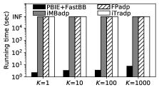
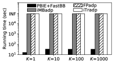
(c) Varying $K$ (DBLP)	(d) Varying $K$ (Google)

Figure 4. Comparison by varying $K$ ($k=1$)

Varying $K$. The results of finding $K$ MaxBPs are shown in Figure 4. PBIE+FastBB outperforms other algorithms by around 2-5 orders of magnitude. Besides, it has the running time clearly rise as $K$ increases compared to other algorithms. Possible reasons include (1) FastBB would explore more MBPs to find the $K$ MaxBPs as $K$ grows and (2) PBIE becomes less effective as $K$ grows. In addition, iTradp has the running time almost not changed with $K$ since it needs to explore almost all MBPs without any powerful pruning.

Varying $k$. The results are shown in Figure 5. PBIE+FastBB significantly outperforms other algorithms by up to five orders of magnitude. In addition, it has the running time first increase and then decrease as $k$ grows. Possible reasons include: (1) the number of $k$-biplexes increases exponentially with $k$, which causes the increase of the running time; (2) the thresholds $\theta_{L}$ and $\theta_{R}$ (i.e., $2k+1$ by default) increase with $k$ and correspondingly the pruning techniques that are based on $\theta_{L}$’s and $\theta_{R}$ become more effective.

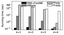
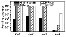
(a) Varying $k$ (Writer)	(b) Varying $k$ (Location)
(c) Varying $k$ (DBLP)	(d) Varying $k$ (Google)

Figure 5. Comparison by varying $k$

Varying $\theta_{L}$ and $\theta_{R}$ thresholds. The results are shown in Figure 6. PBIE+FastBB outperforms all other algorithms by achieving up to around 1000$\times$ speedup. Besides, the running time of all algorithms decreases as $\theta_{L}$ and $\theta_{R}$ grow. The reason is two-fold: (1) the search space (e.g., the number of large $k$-biplexes with the size of each side at least $\theta_{L}$ and $\theta_{R}$) decreases as $\theta_{L}$ and $\theta_{R}$ grow and (2) the pruning rules are more effective for larger $\theta_{L}$’s and $\theta_{R}$’s.

(a) Varying $\theta$ (Writer)	(b) Varying $\theta$ (Location)
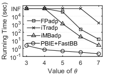
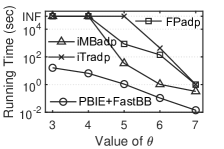
(c) Varying $\theta$ (DBLP)	(d) Varying $\theta$ (Google)

Figure 6. Comparison by varying $\theta=\theta_{L}=\theta_{R}$ ($k=1$)

Varying # of vertices (synthetic datasets). The results are shown in Figure 7(a). PBIE+FastBB outperforms other algorithms by achieving at least 10$\times$ speedup and can handle the largest datasets with 1 million vertices and 10 million edges within INF while others cannot. Besides, the speedup increases as the graph become larger. This is mainly because PBIE would prune more unfruitful vertices when locating the MaxBP in several smaller subgraphs. In addition, the results are well aligned with the theoretical results, i.e., the worst-case time complexity of PBIE+FastBB is exponential wrt $d^{3}$ while that of others is exponential wrt $|V|$. Hence, PBIE+FastBB has larger speed-ups as the graph scale becomes larger (where $d$ remains almost the same due to the fixed edge density, i.e., 20).

Varying edge density (synthetic datasets). The results are shown in Figure 7(b). PBIE+FastBB achieves at least 10$\times$ speedup compared with other algorithms. In addition, the speedup decreases as the graph becomes denser. The reason is that the maximum degree of the bipartite graph, i.e., $d$, increases as the graph becomes denser.

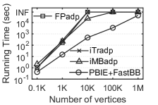
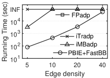
(a) Varying # of vertices	(b) Varying edge density

Figure 7. Comparison on synthetic datasets ($k=1$)

5.2. Performance study

Comparison among various enumeration schemes. We study the effect of various enumeration schemes, namely FastBB, BasicBB, FPadp, iMBadp, and iTradp. We note that all of them are run with the framework PBIE for fair comparison. In particular, BasicBB adopts the classic BK branching and uses the non-decreasing vertex ordering. The results are shown in Figure 8(a) and (b) for varying $k$, and (c) and (d) for varying $\theta=\theta_{L}=\theta_{R}$. First, FastBB outperforms other algorithms, which demonstrates the superiority of proposed Sym-BK branching scheme. Besides, the achieved speedup decreases with $\theta$ since the search space (e.g., the number of large MBPs with the size of each side at least $\theta_{L}$ and $\theta_{R}$) decreases as $\theta_{L}$ and $\theta_{R}$ grow. Second, the algorithms following the BK branching perform better than iTradp that follows a reverse search method. The reason is that the later one cannot be enhanced with effective pruning rules as branch-and-bound algorithms.

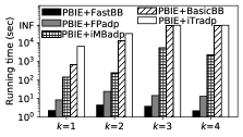
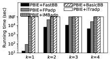
(a) Varying $k$ (DBLP)	(b) Varying $k$ (Google)
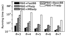
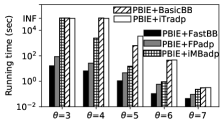
(c) Varying $\theta$ (DBLP, $k$=1)	(d) Varying $\theta$ (Google, $k$=1)

Figure 8. Comparison among various enumeration schemes

Comparison among frameworks. We study the effect of different frameworks and compare four different versions, namely (1) FastBB: without any framework, (2) IE+FastBB: with adapted framework IE, (3) PB+FastBB: with adapted progressive bounding framework PB, and (4) PBIE+FastBB: with proposed combined framework. We note that all frameworks adopt FastBB for fair comparison. The results are shown in Figure 9(a) and (b) for varying $k$, and (c) and (d) for varying $\theta=\theta_{L}=\theta_{R}$. First, both IE+FastBB and PB+FastBB outperform FastBB, which demonstrates the efficiency and scalability of adapted frameworks. Moreover, PBIE+FastBB performs the best and can handle all datasets and settings within INF. This is because PBIE can significantly reduce the size of the original graph (details can be found in the technical report (Yu and Long, 2022) ). Second, PB+FastBB performs better than IE+FastBB. This is because PB can quickly locate the MaxBP at a much smaller subgraph. Third, the speedup decreases as $\theta$ grows. As discussed earlier, the search space gets smaller with $\theta$ and thus the frameworks would have less effects on the running time.

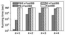
(a) Varying $k$ (DBLP)	(b) Varying $k$ (Google)
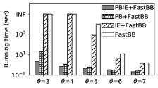
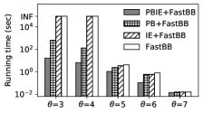
(c) Varying $\theta$ (DBLP, $k$=1)	(d) Varying $\theta$ (Google, $k$=1)

Figure 9. Comparison among frameworks

5.3. Case study: Fraud Detection

We investigate two cohesive models, namely maximal $k$-biplex and maximum $k$-biplex, for a fraud detection task (Hooi et al., 2016) on the Software dataset  (Ni, 2018). The dataset contains 459,436 reviews on 21,663 softwares by 375,147 users. We consider the random camouflage attack scenario (Hooi et al., 2016) where a fraud block with 1K fake users (“K” means a thousand), 1K fake softwares, 50K fake comments, and 50K camouflage comments, is injected to the dataset. Specifically, we randomly generate the fake comments (resp. camouflage comments) between pairs of fake users and fake products (resp. real products). We note that this attack can be easily conducted in reality to help fake users evade the detection, e.g., fake users are coordinated to deliberately post comments on some real products (Hooi et al., 2016). We then find MaxBPs and MBPs from the bipartite graph, and classify all users and products involved in the found subgraphs as fake items and others as real ones.

We measure the running time and F1 score, and show the results in Figure 10 where $\theta_{L}$ is fixed at 4.

• Varying $\theta_{R}$. We find the 2000 MaxBPs (denoted by “MaxBP (2000)”), first-2000 MBPs (denoted by “MBP (2000)”), i.e., the first 2000 MBPs yielded by the algorithm, and all MBPs (denoted by “MBP (All)”) with $\theta_{R}$ varying from 3 to 6, and show the results in Figure 10(a). We have the following observations. (1) MaxBP (2000) achieves the best F1 score (0.99) when $\theta_{R}=5$ among all methods. (2) Both MBP (2000) and MBP (All) achieve their best F1 scores, 0.80 and 0.87, respectively, when $\theta_{R}=5$. (3) Under the setting with the best F1 scores, i.e., $\theta_{R}=5$, MaxBP (2000) and MBP (2000) run comparably fast and both of them run faster than MBP (All). For (1) and (2), the reason could be that the fraud blocks tend to reside in large MBPs with more edges, and for (3), the reason could be that MaxBP (2000) and MBP (2000) need to explore a set of some but not all MBPs.

• Varying $K$. We find the $K$ MaxBPs (denoted by “MaxBP (K)”) and the first-$K$ MBPs (denoted by “MBP (K)”) with $\theta_{R}=5$ since it give the best F1 scores, and show the results in Figure 10(b). We have the following observations. (1) MaxBP (K) has the F1 score higher than MBP (K) on all settings, and achieves the best F1 score at $K=2000$. (2) MaxBP (K) provides a better trade-off between F1 score and running time than MBP (K), e.g., MaxBP (K) provides a F1 score 0.94 with the running time 512 seconds at $K=1000$ while MBP (K) provides a similar F1 score 0.91 with the running time 1512 seconds at $K=16000$.

In summary, MaxBP outperforms MBP for fraud detection in terms of F1 score and the running time, as shown in Figure 10.

We have also explored methods of enumerating maximal bicliques and maximum bicliques for this case study. We found that the best F1-score achieved by enumerating maximal bicliques (with $\theta_{R}=4$) and that of finding the maximum bicliques (with $\theta_{R}=4$) are 0.48 and 0.54, respectively. In particular, when $\theta_{R}\geq 5$, there are few large bicliques, and thus both methods have the recall close to 0. This is mainly because biclique requires full connections among vertices, which is usually too strict.

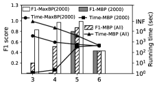
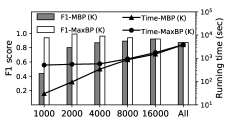
(a) Varying $\theta_{R}$	(b) Varying $K$ ($\theta_{R}=5$)

Figure 10. Case Study: Fraud Detection

6. Related Work

We find that the maximum $k$-biplex search problem was recently studied in (Luo et al., 2022). Some summary of the similarities and differences between (Luo et al., 2022) and our paper include: (1) (Luo et al., 2022) and our paper propose the maximum $k$-biplex search problem concurrently and independently; (2) both (Luo et al., 2022) and our paper prove the NP-hardness of the problem, yet they use different NP complete problems; (3) the solution in (Luo et al., 2022) has the time complexity of $O^{*}(2^{|V|})$ while our FastBB algorithm has the time complexity of $O^{*}(\gamma_{k}^{|V|})$ with $\gamma_{k}<2$; and (4) the solutions in this paper run significantly faster than that in (Luo et al., 2022). Some more details of the comparison can be found in the technical report (Yu and Long, 2022). We review other related work as follows.

Cohesive bipartite structures. Recently, many studies have been conducted on finding cohesive subgraphs of bipartite graphs, including bicliques (Zhang et al., 2014; Abidi et al., 2020; Mukherjee and Tirthapura, 2016; Lyu et al., 2020; Chen et al., 2021; Kloster et al., 2019; Yang et al., 2022), $(\alpha,\beta)$-cores (Liu et al., 2020), quasi-bicliques (Liu et al., 2008; Wang, 2013; Ignatov et al., 2018; Ignatov, 2019), $k$-biplexes (Sim et al., 2009; Yu et al., 2021, 2022), $k$-bitrusses (Zou, 2016; Wang et al., 2020), etc. Biclique is a bipartite graph where any vertex at one side connects all vertices at the other side. Recent works on biclique focus on enumerating maximal bicliques (Zhang et al., 2014; Abidi et al., 2020; Kloster et al., 2019). Given a bipartite graph, $(\alpha,\beta)$-core is the maximal subgraph where any vertex at one side connects a certain number of vertices (i.e., $\alpha$ or $\beta$) at the other side. It has many applications, including recommendation systems (Ding et al., 2017) and community search (Hao et al., 2020; Wang et al., 2021). Existing works of $k$-biplexes focus on enumerating large maximal $k$-biplex (Sim et al., 2009; Yu et al., 2021). A $k$-bitruss (Zou, 2016; Wang et al., 2020) is a bipartite graph where each edge is contained in at least $k$ butterflies, where a butterfly corresponds to a complete 2$\times$2 biclique (Wang et al., 2019). In the literature, there are two types of quasi-biclique, i.e., (1) $\delta$-quasi-biclique (Liu et al., 2008) is a bipartite graph $G(L,R,E)$ where each vertex in $L$ (resp. $R$) misses at most $\delta\cdot|R|$ (resp. $\delta\cdot|L|$) edges with $\delta\in[0,1)$) and (2) $\gamma$-quasi-biclique (Ignatov et al., 2018; Yan et al., 2005) is a bipartite graph $G(L,R,E)$ that can miss at most $\gamma\cdot|L|\cdot|R|$ edges with $\gamma\!\in\![0,1)$. Existing works of quasi-bicliques focus on finding subgraphs with a certain density and degree (Mitzenmacher et al., 2015; Liu et al., 2013). In this paper, we focus on $k$-biplex since it (1) imposes strict enough requirements on connections within a subgraph and tolerates some disconnections and (2) satisfies the hereditary property, which facilitates efficient solutions. In (Yu et al., 2022), a case study of fraud detection on e-commerce platforms is conducted, which shows that $k$-biplex works better than some other cohesive subgraph structures including biclique, $(\alpha,\beta)$-core, and $\delta$-quasi-biclique for the application.

Maximum biclique search. The maximum biclique search problem has attracted much attention in recent years (Dawande et al., 2001; Sözdinler and Özturan, 2018; Lyu et al., 2020; Shaham et al., 2016; Garey and Johnson, 1979; McCreesh and Prosser, 2014; Zhou et al., 2018; Chen et al., 2021; Wang et al., 2018; Yuan et al., 2015; Zhou and Hao, 2017). In general, there are three lines of works, namely maximum edge biclique search (MEBS) (Dawande et al., 2001; Sözdinler and Özturan, 2018; Lyu et al., 2020; Shaham et al., 2016) which finds a biclique $H^{*}$ such that $E(H^{*})$ is maximized, maximum vertex biclique search (MVBS) (Garey and Johnson, 1979) which finds a biclique $H^{*}$ such that $V(H^{*})$ is maximized and maximum balanced biclique search (MBBS) (McCreesh and Prosser, 2014; Zhou et al., 2018; Chen et al., 2021; Wang et al., 2018; Yuan et al., 2015; Zhou and Hao, 2017) which finds a biclique $H^{*}$ such that $V(H^{*})$ is maximized and $L(H^{*})=R(H^{*})$. First, the MEBS problem is NP-hard, for which many techniques have been proposed. Authors in (Dawande et al., 2001; Sözdinler and Özturan, 2018) adopt the integer linear programming techniques to find a MEB, which is not scalable for large bipartite graphs. A recent study (Lyu et al., 2020) proposes a progressive bounding framework to deal with large bipartite graphs. Besides, a Monte Carlo algorithm is proposed in (Shaham et al., 2016), which finds a MEB with a fixed probability. Second, the MVBS problem can be solved in polynomial time by finding a maximum matching (Garey and Johnson, 1979). Third, the MBBS problem is NP-hard, for which both exact methods and approximate methods have been developed. To be specific, exact methods proposed in (McCreesh and Prosser, 2014; Zhou et al., 2018; Chen et al., 2021) are branch-and-bound algorithms which use the widely-used Bron-Kerbosch (BK) branching (Bron and Kerbosch, 1973). Besides, approximate methods include (Wang et al., 2018; Yuan et al., 2015) which introduce a local search framework to find an approximate MBB, (Al-Yamani et al., 2007; Tahoori, 2006) which convert MBBS into a maximum independent set problem and adopt approximate algorithms for the independent set problem, and (Zhou and Hao, 2017) which proposes a heuristic algorithm with tabu search and graph reduction. In summary, there are two types of solutions, namely exact methods and approximate methods. For exact algorithms, most of them follow the branch-and-bound framework and use the BK branching strategy. However, based on our experimental results, BK branching strategy performs worse than our proposed Sym-BK branching strategy for the problem of finding MaxBP. For approximate methods, they cannot be adapted to find the MaxBP exactly.

Maximum quasi-biclique search. The maximum quasi-biclique search problem aims to find a $\gamma$-quasi-biclique or $\delta$-quasi-biclique $H^{*}$ such that $V(H^{*})$ is maximized, which is a NP-hard problem (Liu et al., 2008; Ignatov, 2019). (Ignatov, 2019; Ignatov et al., 2018) use mixed integer programming to find a maximum $\gamma$-quasi-biclique exactly, which cannot handle large datasets. (Wang, 2013; Liu et al., 2008) propose greedy algorithms to find an approximate maximum $\delta$-quasi-biclique, which cannot be adapted to find the MaxBP exactly.

7. Conclusion

In this paper, we study the maximum $k$-biplex search problem, which is to find $K$ maximal $k$-biplexes with the most edges. We propose two branch-and-bound algorithms, among which the better one FastBB is based on a novel Sym-BK branching strategy and achieves better worst-case time complexity than adaptions of existing algorithms. We further develop frameworks to boost the efficiency and scalability of the branch-and-bound algorithms including FastBB. Extensive experiments are conducted on real and synthetic datasets to demonstrate the efficiency of our algorithms and the effectiveness of proposed techniques. In the future, we plan to develop efficient parallel algorithms for the maximum $k$-biplex search problem and explore the possibility of adapting our algorithms to find other types of maximum cohesive subgraphs in bipartite graphs.

8. Proof of Lemma 3

We prove by showing a polynomial reduction from a well-known NP-complete problem, namely maximum clique search, to the maximum $k$-biplex search problem with $\theta_{L}=\theta_{R}=0$, $k=1$, and $K=1$. We define their decision problems as follows.

• CLIQUE: given a general graph $G=(V,E)$ and a positive integer $\alpha$, does $G$ contain a clique with at least $\alpha$ vertices?

• BIPLEX: given a bipartite graph $\mathcal{G}=(\mathcal{L}\cup\mathcal{R},\mathcal{E})$ and two positive integers $k$ and $\alpha^{\prime}$, does $\mathcal{G}$ contain a $k$-biplex with at least $\alpha^{\prime}$ edges?

Let $G=(V,E)$ and $\alpha$ be the inputs of an instance of CLIQUE. W.l.o.g., we assume that $\alpha=\frac{1}{2}|V|$ is a positive integer. This can be achieved with some inflation tricks. Specifically, (1) if the original input $\alpha$ is smaller than $\frac{1}{2}|V|$ (which can be a fractional number), we add to $G$ a new vertex $v$ and $|V|$ edges between $v$ and other vertices. Obviously, every clique would include $v$, increasing $\alpha$ by 1 but $\frac{1}{2}|V|$ by 0.5. (2) If $\alpha>\frac{1}{2}|V|$, we add to $G$ a new vertex $v$ with no edges. Clearly, every clique would not include $v$, increasing $\frac{1}{2}|V|$ by 0.5 only. By repeating above two steps, we can make $\alpha=\frac{1}{2}|V|$ finally.

Now, we construct an instance of BIPLEX (with $k=1$) with $\mathcal{G}=(\mathcal{L}\cup\mathcal{R},\mathcal{E})$ and $\alpha^{\prime}$. To be specific,

$$\mathcal{L}=V\text{ and }\mathcal{R}=E\cup W\cup U,\ |W|=\frac{1}{2}\alpha(\alpha-5),\ |U|=2\alpha$$

where $W\cup U$ is a set of new elements and $|V|=2\alpha$. Assume $V=\{v_{1},...,v_{2\alpha}\}$ and $U=\{u_{1},...,u_{2\alpha}\}$. We have

$$\mathcal{E}=\mathcal{E}(\mathcal{G}[V\cup E])\cup\mathcal{E}(\mathcal{G}[V\cup W])\cup\mathcal{E}(\mathcal{G}[V\cup U])$$

$$=\{(v,e)\mid v\in V,e\in E,v\notin e\}\cup\{(v,w)\mid v\in V,w\in W\}$$

$$\cup\{(v_{i},u_{j})\mid v_{i}\in V,u_{j}\in U,i\neq j\},$$

$$\alpha^{\prime}=\frac{1}{2}\alpha^{3}+\frac{3}{2}\alpha^{2}-\alpha.$$

To guarantee $|W|\geq 0$, we assume $\alpha\geq 5$ which can be achieved with the inflation tricks. The above construction can be finished in polynomial time.

We then show that $G$ has a clique with at least $\alpha$ vertices iff $\mathcal{G}$ has a 1-biplex with at least $\alpha^{\prime}$ edges. We consider the following two cases.

Case 1: $G$ has a clique $G[C]$ with $\alpha$ vertices, i.e., $C\subseteq V$ and $|C|=\alpha$. Consider $X=V\backslash C$ and $Y=E(G[C])\cup W\cup U$. We prove this case by showing that $\mathcal{G}[X\cup Y]$ is a 1-biplex with $\alpha^{\prime}$ edges. To be specific, for each vertex $v\in X$, we know: (1) vertex $v$ connects all vertices from $E(G[C])$ since $v$ is not an endpoint of any edge in $E(G[C])$, thereby yielding $|X|\times|E(G[C])|$ edges in total; (2) vertex $v$ connects all vertices from $W$ based on the construction, yielding $|X|\times|W|$ edges in total; and (3) vertex $v$ disconnects exactly one vertex in $U$ based on the construction, yielding $|X|\times(|U|-1)$ edges in total. For each vertex $u\in Y$, we can similarly verify that vertex $u$ disconnects no more than one vertex from $X$. In summary, we have a 1-biplex $\mathcal{G}[X\cup Y]$ with

$$|\mathcal{E}(\mathcal{G}[X\cup Y])|=|X|\times|E(G[C])|+|X|\times|W|+|X|\times(|U|-1),$$

where $|X|=\alpha$, $|E(G[C])|=\frac{1}{2}\alpha(\alpha-1)$, $|W|=\frac{1}{2}\alpha(\alpha-5)$ and $|U|=2\alpha$. Therefore, $|\mathcal{E}(\mathcal{G}[X\cup Y])|$ is exactly $\alpha^{\prime}$.

Case 2: $G$ does not have a clique with at least $\alpha$ vertices. If no 1-biplex is found in $\mathcal{G}$, the proof is finished. Otherwise, let $\mathcal{G}[X\cup Y]$ be an arbitrary 1-biplex in $\mathcal{G}$ such that $X\subseteq\mathcal{L}$ and $Y\subseteq\mathcal{R}$. We finish the proof by showing that $|\mathcal{E}(\mathcal{G}[X\cup Y])|<\alpha^{\prime}$. To estimate $|\mathcal{E}(\mathcal{G}[X\cup Y])|$, we divide $Y$ into two disjoint parts $Y_{0}\cup Y_{1}$, i.e., vertices in $Y_{0}$ connect all vertices from $X$ and vertices in $Y_{1}$ disconnect exactly one vertex from $X$. For $Y_{0}$, we have: (1) it includes all vertices from $E(G[V\backslash X])\subseteq E$ since every edge in $E(G[V\backslash X])$ has no endpoint in $X$; (2) it includes all vertices from $W$ based on our construction; and (3) it includes $|V\backslash X|$ vertices from $U$ (with $X=\{v_{1},...,v_{|X|}\}$, vertices in $\{u_{|X|+1},...,u_{2\alpha}\}$ would connect all vertices from $X$ based on our construction). For $Y_{1}$, it includes at most $|X|$ vertices since otherwise there exists at least a vertex in $X$ that disconnects at least 2 vertices based on the pigeonhole principle. This contradicts to the definition of 1-biplex $\mathcal{G}[X\cup Y]$. In summary, we have

$$|\mathcal{E}(\mathcal{G}[X\cup Y])|=|X|\times|Y_{0}|+(|X|-1)\times|Y_{1}|\ \ \ \ \ \$$

(14) $$\leq|X|\!\times\!(|E(G[V\backslash X])|\!+\!|W|\!+\!|V\backslash X|)+(|X|\!-\!1)\!\times\!|X|$$

Let $x=|X|$. We have $0\leq x\leq 2\alpha$ and consider two cases.

Case 2.1: $\alpha<x\leq 2\alpha$. Let $y=x-\alpha$ ($0<y\leq\alpha$). We have $|X|=\alpha+y$ and $|V\backslash X|=\alpha-y$. Moreover, we can obtain $|E(G[V\backslash X])|\leq\frac{1}{2}|V\backslash X|(|V\backslash X|-1)=\frac{1}{2}(\alpha-y)(\alpha-y-1)$ where the equality holds iff $G[V\backslash X]$ is a clique. According to equation (8), we have $|\mathcal{E}(\mathcal{G}[X\cup Y])|\leq(\alpha+y)[\frac{1}{2}(\alpha-y)(\alpha-y-1)+\frac{1}{2}\alpha^{2}-\frac{5}{2}\alpha+2\alpha-(\alpha+y)]+(\alpha+y-1)(\alpha+y)$ which reduces to

$$|\mathcal{E}(\mathcal{G}[X\cup Y])|-\alpha^{\prime}\leq\frac{1}{2}y[y^{2}-(\alpha-1)y-\alpha-2].$$

It is easy to verify that $y^{2}-(\alpha-1)y-\alpha-2$ is negative for $0\leq y\leq\alpha$. Therefore, we have $|\mathcal{E}(\mathcal{G}[X\cup Y])|<\alpha^{\prime}$.

Case 2.2: $0\leq x\leq\alpha$. Let $y=\alpha-x$ ($0\leq y\leq\alpha$). We have $|X|=\alpha-y$ and $|V\backslash X|=\alpha+y$. Since $|V\backslash X|=2\alpha-x\geq\alpha$ and $G$ does not have a clique with at least $\alpha$ vertices, it is easy to verify that $|E(G[V\backslash X])|<\frac{1}{2}|V\backslash X|(|V\backslash X|-1)-y$ since otherwise there exists a clique with at least $\alpha$ vertices in $G$ (note that the right term can be regarded as a process of iteratively removing $y$ edges from a clique with $|V\backslash X|$ vertices and after removing an edge, the maximum clique in the remaining graph has its size decrease by at most 1, which yields a clique with $|V\backslash X|-y=\alpha+y-y=\alpha$ vertices). According to equation (8), we have $|\mathcal{E}(\mathcal{G}[X\cup Y])|<(\alpha-y)[\frac{1}{2}(\alpha+y)(\alpha+y-1)-y+\frac{1}{2}\alpha^{2}-\frac{5}{2}\alpha+2\alpha-(\alpha-y)]+(\alpha-y-1)(\alpha-y)$ which reduces to

$$|\mathcal{E}(\mathcal{G}[X\cup Y])|-\alpha^{\prime}<\frac{1}{2}y[-y^{2}-(\alpha-3)y-\alpha+2].$$

It is easy to verify that $y[-y^{2}-(\alpha-3)y-\alpha+2]\leq 0$ for $0\leq y\leq\alpha$ and $\alpha\geq 5$. We thus have $|\mathcal{E}(\mathcal{G}[X\cup Y])|<\alpha^{\prime}$.

9. Acknowledgement

The research is supported by the Ministry of Education, Singapore, under its Academic Research Fund (Tier 2 Award MOE-T2EP20221-0013 and Tier 1 Award (RG77/21)). Any opinions, findings and conclusions or recommendations expressed in this material are those of the author(s) and do not reflect the views of the Ministry of Education, Singapore.

References

- (1)
- Abidi et al. (2020) Aman Abidi, Rui Zhou, Lu Chen, and Chengfei Liu. 2020. Pivot-based Maximal Biclique Enumeration. In Proc. Int. Joint Conf. Artif. Intell., IJCAI 2020. 3558–3564.
- Al-Yamani et al. (2007) Ahmad A. Al-Yamani, S. Ramsundar, and Dhiraj K. Pradhan. 2007. A Defect Tolerance Scheme for Nanotechnology Circuits. IEEE Trans. Circuits Syst. I Regul. Pap. 54-I, 11 (2007), 2402–2409.
- Beutel et al. (2013) Alex Beutel, Wanhong Xu, Venkatesan Guruswami, Christopher Palow, and Christos Faloutsos. 2013. Copycatch: stopping group attacks by spotting lockstep behavior in social networks. In Proceedings of the 22nd international conference on World Wide Web. 119–130.
- Bron and Kerbosch (1973) Coen Bron and Joep Kerbosch. 1973. Algorithm 457: finding all cliques of an undirected graph. Commun. ACM 16, 9 (1973), 575–577.
- Chen et al. (2021) Lu Chen, Chengfei Liu, Rui Zhou, Jiajie Xu, and Jianxin Li. 2021. Efficient Exact Algorithms for Maximum Balanced Biclique Search in Bipartite Graphs. In Proc. ACM SIGMOD Int. Conf. Manage. Data. 248–260.
- Cohen et al. (2008) Sara Cohen, Benny Kimelfeld, and Yehoshua Sagiv. 2008. Generating all maximal induced subgraphs for hereditary and connected-hereditary graph properties. J. Comput. Syst. Sci. 74, 7 (2008), 1147–1159.
- Conte et al. (2018) Alessio Conte, Tiziano De Matteis, Daniele De Sensi, Roberto Grossi, Andrea Marino, and Luca Versari. 2018. D2K: Scalable Community Detection in Massive Networks via Small-Diameter k-Plexes. In Proc. 24th ACM SIGKDD Int. Conf. Knowl. Discovery Data Mining. 1272–1281.
- Dawande et al. (2001) Milind Dawande, Pinar Keskinocak, Jayashankar M Swaminathan, and Sridhar Tayur. 2001. On bipartite and multipartite clique problems. Journal of Algorithms 41, 2 (2001), 388–403.
- Ding et al. (2017) Danhao Ding, Hui Li, Zhipeng Huang, and Nikos Mamoulis. 2017. Efficient fault-tolerant group recommendation using alpha-beta-core. In Proceedings of the 2017 ACM on Conference on Information and Knowledge Management. 2047–2050.
- Gangireddy et al. (2020) Siva Charan Reddy Gangireddy, Cheng Long, and Tanmoy Chakraborty. 2020. Unsupervised Fake News Detection: A Graph-based Approach. In Proceedings of the 31st ACM Conference on Hypertext and Social Media. 75–83.
- Garey and Johnson (1979) Michael R Garey and David S Johnson. 1979. Computers and intractability. Vol. 174. freeman San Francisco.
- Günnemann et al. (2011) Stephan Günnemann, Emmanuel Müller, Sebastian Raubach, and Thomas Seidl. 2011. Flexible Fault Tolerant Subspace Clustering for Data with Missing Values. In 11th IEEE International Conference on Data Mining, ICDM 2011. 231–240.
- Hao et al. (2020) Yang Hao, Mengqi Zhang, Xiaoyang Wang, and Chen Chen. 2020. Cohesive Subgraph Detection in Large Bipartite Networks. In SSDBM 2020: 32nd International Conference on Scientific and Statistical Database Management. ACM, 22:1–22:4.
- Hooi et al. (2016) Bryan Hooi, Hyun Ah Song, Alex Beutel, Neil Shah, Kijung Shin, and Christos Faloutsos. 2016. FRAUDAR: Bounding Graph Fraud in the Face of Camouflage. In Proc. ACM SIGKDD Int. Conf. Knowl. Discov. Data Mining. ACM, 895–904.
- Ignatov (2019) Dmitry I. Ignatov. 2019. Preliminary Results on Mixed Integer Programming for Searching Maximum Quasi-Bicliques and Large Dense Biclusters. In Supplementary Proceedings of ICFCA 2019 Conference and Workshops (CEUR Workshop Proceedings, Vol. 2378). CEUR-WS.org, 28–32.
- Ignatov et al. (2018) Dmitry I Ignatov, Polina Ivanova, and Albina Zamaletdinova. 2018. Mixed Integer Programming for Searching Maximum Quasi-Bicliques. In International Conference on Network Analysis. Springer, 19–35.
- Kloster et al. (2019) Kyle Kloster, Blair D Sullivan, and Andrew van der Poel. 2019. Mining maximal induced bicliques using odd cycle transversals. In Proceedings of the 2019 SIAM International Conference on Data Mining. SIAM, 324–332.
- Liu et al. (2020) Boge Liu, Long Yuan, Xuemin Lin, Lu Qin, Wenjie Zhang, and Jingren Zhou. 2020. Efficient (,)-core computation in bipartite graphs. The VLDB Journal 29, 5 (2020), 1075–1099.
- Liu et al. (2013) Hsiao-Fei Liu, Chung-Tsai Su, and An-Chiang Chu. 2013. Fast Quasi-biclique Mining with Giraph. In IEEE International Congress on Big Data, BigData Congress 2013. IEEE Computer Society, 347–354.
- Liu et al. (2008) Xiaowen Liu, Jinyan Li, and Lusheng Wang. 2008. Quasi-bicliques: Complexity and Binding Pairs. In Computing and Combinatorics, 14th Annual International Conference, COCOON 2008, Vol. 5092. Springer, 255–264.
- Luo et al. (2022) Wensheng Luo, Kenli Li, Xu Zhou, Yunjun Gao, and Keqin Li. 2022. Maximum Biplex Search over Bipartite Graphs. In 2022 IEEE 38th International Conference on Data Engineering (ICDE). IEEE, 898–910.
- Lyu et al. (2020) Bingqing Lyu, Lu Qin, Xuemin Lin, Ying Zhang, Zhengping Qian, and Jingren Zhou. 2020. Maximum biclique search at billion scale. Proceedings of the VLDB Endowment (2020).
- McCreesh and Prosser (2014) Ciaran McCreesh and Patrick Prosser. 2014. An Exact Branch and Bound Algorithm with Symmetry Breaking for the Maximum Balanced Induced Biclique Problem. In Integration of AI and OR Techniques in Constraint Programming International Conference, Helmut Simonis (Ed.), Vol. 8451. Springer, 226–234.
- Mitzenmacher et al. (2015) Michael Mitzenmacher, Jakub Pachocki, Richard Peng, Charalampos E. Tsourakakis, and Shen Chen Xu. 2015. Scalable Large Near-Clique Detection in Large-Scale Networks via Sampling. In Proc. ACM SIGKDD Int. Conf. Knowl. Discov. Data Mining. ACM, 815–824.
- Mukherjee and Tirthapura (2016) Arko Provo Mukherjee and Srikanta Tirthapura. 2016. Enumerating maximal bicliques from a large graph using mapreduce. IEEE Transactions on Services Computing 10, 5 (2016), 771–784.
- Ni (2018) Jianmo Ni. 2018. Amazon Review Data. https://nijianmo.github.io/amazon/index.html
- Poernomo and Gopalkrishnan (2009) Ardian Kristanto Poernomo and Vivekanand Gopalkrishnan. 2009. Towards efficient mining of proportional fault-tolerant frequent itemsets. In Proc. ACM SIGKDD Int. Conf. Knowl. Discov. Data Mining. 697–706.
- Shaham et al. (2016) Eran Shaham, Honghai Yu, and Xiao-Li Li. 2016. On finding the maximum edge biclique in a bipartite graph: a subspace clustering approach. In Proceedings of the 2016 SIAM International Conference on Data Mining. SIAM, 315–323.
- Sim et al. (2009) Kelvin Sim, Jinyan Li, Vivekanand Gopalkrishnan, and Guimei Liu. 2009. Mining maximal quasi-bicliques: Novel algorithm and applications in the stock market and protein networks. Statistical Analysis and Data Mining 2, 4 (2009), 255–273.
- Sözdinler and Özturan (2018) Melih Sözdinler and Can Özturan. 2018. Finding Maximum Edge Biclique in Bipartite Networks by Integer Programming. In 2018 IEEE International Conference on Computational Science and Engineering (CSE). IEEE, 132–137.
- Tahoori (2006) Mehdi Baradaran Tahoori. 2006. Application-independent defect tolerance of reconfigurable nanoarchitectures. ACM J. Emerg. Technol. Comput. Syst. 2, 3 (2006), 197–218.
- Wang et al. (2006) Jun Wang, Arjen P De Vries, and Marcel JT Reinders. 2006. Unifying user-based and item-based collaborative filtering approaches by similarity fusion. In Proceedings of the 29th annual international ACM SIGIR conference on Research and development in information retrieval. 501–508.
- Wang et al. (2019) Kai Wang, Xuemin Lin, Lu Qin, Wenjie Zhang, and Ying Zhang. 2019. Vertex Priority Based Butterfly Counting for Large-scale Bipartite Networks. Proc. VLDB Endow. 12, 10 (2019), 1139–1152.
- Wang et al. (2020) Kai Wang, Xuemin Lin, Lu Qin, Wenjie Zhang, and Ying Zhang. 2020. Efficient Bitruss Decomposition for Large-scale Bipartite Graphs. In Proc. 36th IEEE Int. Conf. Data Eng., ICDE 2020. IEEE, 661–672.
- Wang et al. (2021) Kai Wang, Wenjie Zhang, Xuemin Lin, Ying Zhang, Lu Qin, and Yuting Zhang. 2021. Efficient and Effective Community Search on Large-scale Bipartite Graphs. In Proc. 36th IEEE Int. Conf. Data Eng., ICDE 2021. IEEE, 85–96.
- Wang (2013) Lusheng Wang. 2013. Near optimal solutions for maximum quasi-bicliques. Journal of Combinatorial Optimization 25, 3 (2013), 481–497.
- Wang et al. (2018) Yiyuan Wang, Shaowei Cai, and Minghao Yin. 2018. New heuristic approaches for maximum balanced biclique problem. Information Sciences 432 (2018), 362–375.
- Wang et al. (2017) Zhuo Wang, Qun Chen, Boyi Hou, Bo Suo, Zhanhuai Li, Wei Pan, and Zachary G Ives. 2017. Parallelizing maximal clique and k-plex enumeration over graph data. J. Parallel and Distrib. Comput. 106 (2017), 79–91.
- Wang et al. (2022) Zhengren Wang, Yi Zhou, Mingyu Xiao, and Bakhadyr Khoussainov. 2022. Listing Maximal k-Plexes in Large Real-World Graphs. In Proceedings of the ACM Web Conference 2022. 1517–1527.
- Yan et al. (2005) Changhui Yan, J Gordon Burleigh, and Oliver Eulenstein. 2005. Identifying optimal incomplete phylogenetic data sets from sequence databases. Molecular phylogenetics and evolution 35, 3 (2005), 528–535.
- Yang et al. (2022) Jianye Yang, Yun Peng, and Wenjie Zhang. 2022. (p,q)-biclique counting and enumeration for large sparse bipartite graphs. Proceedings of the VLDB Endowment (2022).
- Yu and Long (2021) Kaiqiang Yu and Cheng Long. 2021. Graph Mining Meets Fake News Detection. In Data Science for Fake News. Springer, 169–189.
- Yu and Long (2022) Kaiqiang Yu and Cheng Long. 2022. Maximum -Biplex Search on Bipartite Graphs: A Symmetric-BK Branching Approach (Technical report). https://personal.ntu.edu.sg/c.long/paper/23-SIGMOD-MaxBP-report.pdf.
- Yu et al. (2021) Kaiqiang Yu, Cheng Long, P Deepak, and Tanmoy Chakraborty. 2021. On Efficient Large Maximal Biplex Discovery. IEEE Transactions on Knowledge and Data Engineering (2021).
- Yu et al. (2022) Kaiqiang Yu, Cheng Long, Shengxin Liu, and Da Yan. 2022. Efficient Algorithms for Maximal -Biplex Enumeration. In Proc. ACM SIGMOD Int. Conf. Manage. Data. 860–873.
- Yuan et al. (2015) Bo Yuan, Bin Li, Huanhuan Chen, and Xin Yao. 2015. A New Evolutionary Algorithm with Structure Mutation for the Maximum Balanced Biclique Problem. IEEE Trans. Cybern. 45, 5 (2015), 1040–1053.
- Zhang and Ghorbani (2020) Xichen Zhang and Ali A Ghorbani. 2020. An overview of online fake news: Characterization, detection, and discussion. Information Processing & Management 57, 2 (2020), 102025.
- Zhang et al. (2014) Yun Zhang, Charles A Phillips, Gary L Rogers, Erich J Baker, Elissa J Chesler, and Michael A Langston. 2014. On finding bicliques in bipartite graphs: a novel algorithm and its application to the integration of diverse biological data types. BMC bioinformatics 15, 1 (2014), 110.
- Zhou and Hao (2017) Yi Zhou and Jin-Kao Hao. 2017. Combining tabu search and graph reduction to solve the maximum balanced biclique problem. CoRR abs/1705.07339 (2017).
- Zhou et al. (2018) Yi Zhou, André Rossi, and Jin-Kao Hao. 2018. Towards effective exact methods for the Maximum Balanced Biclique Problem in bipartite graphs. European Journal of Operational Research 269, 3 (2018), 834–843.
- Zhou et al. (2020) Yi Zhou, Jingwei Xu, Zhenyu Guo, Mingyu Xiao, and Yan Jin. 2020. Enumerating Maximal k-Plexes with Worst-Case Time Guarantee. In The Thirty-Fourth AAAI Conference on Artificial Intelligence, AAAI 2020. 2442–2449.
- Zou (2016) Zhaonian Zou. 2016. Bitruss Decomposition of Bipartite Graphs. In Database Systems for Advanced Applications - 21st International Conference, DASFAA 2016, Vol. 9643. Springer, 218–233.