On the Role of Data Homogeneity in Multi-Agent Non-convex Stochastic Optimization

Abstract

This paper studies the role of data homogeneity on multi-agent optimization. Concentrating on the decentralized stochastic gradient (DSGD) algorithm, we characterize the transient time, defined as the minimum number of iterations required such that DSGD can achieve the comparable performance as its centralized counterpart. When the Hessians for the objective functions are identical at different agents, we show that the transient time of DSGD is ${\cal O}(n^{4/3}/\rho^{8/3})$ for smooth (possibly non-convex) objective functions, where $n$ is the number of agents and $\rho$ is the spectral gap of connectivity graph. This is improved over the bound of ${\cal O}(n^{2}/\rho^{4})$ without the Hessian homogeneity assumption. Our analysis leverages a property that the objective function is twice continuously differentiable. Numerical experiments are presented to illustrate the essence of data homogeneity to fast convergence of DSGD.

I Introduction

Consider a system of $n$ agents which are connected on a network. We are concerned with the following multi-agent stochastic optimization problem:

$$\textstyle\min_{\bm{\theta}\in\mathbb{R}^{d}}f(\bm{\theta}):=(1/n)\sum_{i=1}^{n}f_{i}(\bm{\theta}),$$ (1)

where $f_{i}:\mathbb{R}^{d}\to\mathbb{R}$, $d\in\mathbb{N}$, is the local stochastic objective function held by agent $i$, $i=1,\ldots,n$. The gradient of each function $f_{i}(\bm{\theta})$ is assumed to be Lipschitz continuous with respect to (w.r.t.) the decision variable $\bm{\theta}\in\mathbb{R}^{d}$ while the function itself is possibly non-convex. In addition, the $n$ agents communicate with neighboring agents through an undirected graph as they tackle (1) in a collaborative fashion.

The multi-agent optimization problem (1) has wide applications in control and machine learning (ML) [1, 2, 3]. We concentrate on the distributed ML application. The function $f_{i}(\bm{\theta})$ models the mismatch of the decision variable $\bm{\theta}\in\mathbb{R}^{d}$ with respect to the local data held by the $i$th agent. Concretely, we consider objective function of the form

$$f_{i}(\bm{\theta})=\mathbb{E}_{z_{i}\sim{\sf B}_{i}}[\ell(\bm{\theta};z_{i})],$$ (2)

where the data distribution ${\sf B}_{i}$ is defined on the space ${\sf Z}$ as it describes the data at the $i$th agent, and $\ell:\mathbb{R}^{d}\times{\sf Z}\to\mathbb{R}$ is the loss function. We remark that in distributed ML, a common setting is to assume homogeneous data such that ${\sf B}_{i}={\sf B}_{j}$ for all $i,j$. The latter models a scenario with $f_{i}(\bm{\theta})\equiv f_{j}(\bm{\theta})$ where agents observe independent and identically distributed (i.i.d.) samples [4, 5]. Note this is in contrast to the non-i.i.d. setting where heterogeneous data is observed [6].

This paper focuses on tackling (1) via stochastic distributed first-order algorithms. In the basic setting, each agent carries out the optimization of a local estimate of a stationary solution to (1) using noisy gradients of its local objective function $f_{i}(\bm{\theta})$. The latter is assumed to be unbiased estimates of ${\nabla}f_{i}(\bm{\theta})$ with bounded second order moment. Particularly, the distributed stochastic gradient (DSGD) method is proposed in [7] (also see [1]) which combines network average consensus with stochastic gradient updates. Despite its simple structure, DSGD is shown to be efficient theoretically and empirically in tackling large-scale machine learning problems. In particular, [8] showed that DSGD achieves a ‘linear speedup’ where the asymptotic convergence rate approaches that of a centralized SGD (CSGD) algorithm with a minibatch size of $n$, i.e., with reduced variance.

However, the convergence rate of DSGD can be severely affected by the network size $n$, the mixing rate (a.k.a. spectral gap) of the connection graph $\rho\in(0,1]$ (see A1). In fact, [8] demonstrated that the linear speedup of DSGD can be guaranteed only when the iteration number exceeds a transient time of ${\cal O}(n^{2}/\rho^{4})$ iterations, which can be undesirable for system with many agents; also see the recent work [9] which focused on strongly convex optimization problems. Note that we have $\rho=\Theta(1/n^{2})$ for ring graph, $\rho=\Theta(1/n)$ for 2d-torus graph, see [10]. The study of the transient time is important where it is closely linked to the communication efficiency in distributed optimization.

Recent works have sought to speed up the convergence of distributed stochastic optimization by designing new and sophisticated algorithms. Examples include [11, 12] which apply multiple communication steps per iteration, D-GET, GT-HSGD [13, 14] which combine gradient tracking with variance reduction, EDAS [15] which utilizes a similar idea to EXTRA [16] but characterizes an improved transient time for strongly convex problems. We also mention that recent works have combined compressed communication in distributed optimization, e.g., [17, 18], whose techniques are complementary to the above works.

This paper is motivated by the successes of DSGD in practice shown in various works [8, 19, 20]. We depart from the prior studies and inquire the following question:

Can DSGD achieve fast convergence with a shorter transient time than ${\cal O}(n^{2}/\rho^{4})$?

We provide an affirmative answer to the above question through studying the role of data homogeneity in distributed stochastic optimization. Our key finding is that when the data held by agents are (close to) homogeneous such that the Hessians are close, i.e., ${\nabla}^{2}f_{i}(\bm{\theta})\approx{\nabla}^{2}f_{j}(\bm{\theta})$ for any $i,j$ and $\bm{\theta}\in\mathbb{R}^{d}$, then the transient time of DSGD can be significantly shortened. To summarize, our contributions are:

• Under the Hessian homogeneity assumption and a second order smoothness condition for the objective function $f_{i}$, we show that the transient time of DSGD can be improved to ${\cal O}(n^{4/3}/\rho^{8/3})$ from ${\cal O}(n^{2}/\rho^{4})$ in [8]. Our result highlights the role of data homogeneity in the (fast) convergence of DSGD which may explain the latter’s efficacy in practical large-scale machine learning.

• We introduce new proof techniques for finding tight bounds in the convergence of distributed stochastic optimization. Importantly, we demonstrate how to extract accelerated convergence rates when the Hessians of objective functions are Lipschitz. This leads to a set of high order inequalities with fast-decaying errors.

• To verify our theorems, we conduct numerical experiment on a toy binary classification problem with linear models. We empirically demonstrate that data homogeneity is a key factor affecting the (fast) convergence of DSGD through a controlled comparison between DSGD with homogeneous and heterogeneous data.

To our best knowledge, this is the first analysis to demonstrate accelerated convergence rate without modifying the simple structure of DSGD. Our result provides evidence for the good performance of DSGD in practice.

Notations: Throughout this paper, we use the following notations: $\left\|\cdot\right\|$ is the vector $\ell_{2}$ norm or the matrix spectral norm depending on the argument, $\left\|\cdot\right\|_{F}$ is the matrix Frobenius norm, and ${\bm{1}}$ is the all-one column vector in $\mathbb{R}^{n}$. We set $f^{\star}\mathrel{\mathop{:}}=\min_{\bm{\theta}\in\mathbb{R}^{d}}f(\bm{\theta})>-\infty$ as the optimal objective value of (1). The subscript-less operator $\mathbb{E}[\cdot]$ denotes the total expectation taken over all randomnesses in the operand.

II Problem Statement and Assumptions

Consider a multiagent network system whose communication is represented by an undirected graph ${\cal G}=({\cal N},{\cal E})$, where ${\cal N}=[n]=\{1,\ldots,n\}$ is the set of agents and ${\cal E}\subseteq{\cal N}\times{\cal N}$ denotes the set of edges between the communicating agents. Note that $(i,i)\in{\cal E}$ as self loops are included in ${\cal G}$. Every agent $i\in{\cal N}$ can directly receive and send information only from its neighbors $\{j:(i,j)\in{\cal E}\}$.

Furthermore, the graph ${\cal G}$ is endowed with a symmetric, weighted adjacency matrix (a.k.a. mixing matrix) ${\bm{W}}\in\mathbb{R}^{n\times n}$ such that $W_{ij}=W_{ji}>0$ if and only if $(i,j)\in{\cal E}$; otherwise $W_{ij}=W_{ji}=0$. Moreover, we assume that

A​ 1.

The matrix ${\bm{W}}\in\mathbb{R}^{n\times n}$ is doubly stochastic, i.e., ${\bm{W}}\mathbf{1}={\bm{W}}^{\top}\mathbf{1}=\mathbf{1}$. There exists a constant ${\rho}\in(0,1]$ and a projection matrix ${\bm{U}}\in\mathbb{R}^{n\times(n-1)}$ which can be represented as $\bm{I}-\frac{1}{n}\mathbf{1}\mathbf{1}^{\top}={\bm{U}}{\bm{U}}^{\top}$ such that $\left\|{\bm{U}}^{\top}\bm{W}\bm{U}\right\|_{2}\leq 1-{\rho}$.

The above is a common assumption for the connected graph ${\cal G}$. For instance, the mixing matrix ${\bm{W}}$ satisfying A1 can be constructed using the Metropolis-Hasting weights [10].

To tackle (1), a classical algorithm is the decentralized stochastic gradient descent (DSGD), whose recursion at iteration $t\geq 0$ can be described as

$$\bm{\theta}_{i}^{t+1}=\sum_{j=1}^{n}W_{ij}\bm{\theta}_{j}^{t}-\gamma_{t+1}{{\nabla}}\ell(\bm{\theta}_{i}^{t};z_{i}^{t+1}),~{}i=1,\ldots,n,$$ (3)

where $z_{i}^{t+1}\sim{\sf B}_{i}$ is a sample drawn independently from the distribution ${\sf B}_{i}$, and $\gamma_{t+1}>0$ is the step size.

The DSGD algorithm (3) is a gossip type algorithm where information is spread along the edges on the communication graph ${\cal G}$. At iteration $t$, the local iterate $\bm{\theta}_{i}^{t}$ held by agent $i$ is communicated to the neighboring nodes $j$. Each agent $i$ performs a consensus update by computing an average of its local iterate as well as the neighbors’ iterates via the mixing matrix ${\bm{W}}$. Subsequently, the agent draws a stochastic gradient estimate ${\nabla}\ell(\bm{\theta}_{i}^{t};z_{i}^{t+1})$ to perform a gradient step.

II-A Convergence of DSGD: Basic Results

We first discuss a basic convergence result for DSGD which is derived under a general setting that does not require the data across agents in the model (1) to be homogeneous. Notice that our result below is akin to the analysis in [8].

Our result depends on a few standard assumptions, which have been used in prior works such as [8], as follows:

A​ 2.

For any $i=1,...,n$, there exists $L\geq 0$ such that

$$\|{\nabla}f_{i}(\bm{\theta}^{\prime})-{\nabla}f_{i}(\bm{\theta})\|\leq L\|\bm{\theta}^{\prime}-\bm{\theta}\|,~{}\forall~{}\bm{\theta}^{\prime},\bm{\theta}\in\mathbb{R}^{d}.$$ (4)

The above assumes that the gradient of each local objective function is $L$-Lipschitz continuous. Note that under the above assumption, $f_{i}(\bm{\theta})$ can be non-convex.

A​ 3.

For any $i=1,\ldots,n$ and fixed $\bm{\theta}\in\mathbb{R}^{d}$, it holds $\mathbb{E}_{z_{i}\sim{\sf B}_{i}}[{\nabla}\ell(\bm{\theta};z_{i})]={\nabla}f_{i}(\bm{\theta})$ and there exists $\sigma\geq 0$ with

$$\mathbb{E}_{z_{i}\sim{\sf B}_{i}}[\|{\nabla}\ell(\bm{\theta};z_{i})-{\nabla}f_{i}(\bm{\theta})\|^{2}]\leq\sigma^{2}.$$ (5)

A​ 4.

For any $i=1,\ldots,n$, there exists $\varsigma\geq 0$ such that:

$$\|{\nabla}f(\bm{\theta})-{\nabla}f_{i}(\bm{\theta})\|\leq\varsigma,~{}\forall~{}\bm{\theta}\in\mathbb{R}^{d}.$$ (6)

In the above, A3 states that the stochastic gradient estimates are unbiased and have bounded variance. Meanwhile, A4 assumes that the gradients of the component function, ${\nabla}f_{i}(\bm{\theta})$, have bounded distance from the gradient of the average function, ${\nabla}f(\bm{\theta})$. Notice that the scalar $\varsigma$ measures the amount of data homogeneity (via gradient). If $\varsigma=0$, then $f_{i}(\bm{\theta}),f_{j}(\bm{\theta})$ differ only by a constant; see [8].

It will be convenient to denote the averaged iterate at the $t$th iteration as:

$$\textstyle\overline{\bm{\theta}}^{t}:=(1/n)\sum_{i=1}^{n}\bm{\theta}_{i}^{t}.$$ (7)

Observe the following basic convergence results for DSGD:

Theorem 1.

Under A1–4, suppose that there exists $b\in\mathbb{R}_{+}$ such that

$$\textstyle\sup_{t\geq 1}\gamma_{t}\leq\min\left\{\frac{\rho}{4L},\sqrt{\frac{\rho/(4b)}{1-\rho/2}}\right\},~{}\frac{\gamma_{t}}{\gamma_{t+1}}\leq 1+b\gamma_{t+1}.$$

Let ${\sf D}\mathrel{\mathop{:}}=f(\overline{\bm{\theta}}^{0})-f^{\star}$. For any $T\geq 1$, it holds

$$\textstyle\mathbb{E}\left[\sum_{t=0}^{T-1}\gamma_{t+1}\left\|{\nabla}f(\overline{\bm{\theta}}^{t})\right\|^{2}\right]$$ (8)

$$\leq 4{\sf D}+\frac{2L\sigma^{2}}{n}\sum_{t=0}^{T-1}\gamma_{t+1}^{2}+\frac{32L^{2}(\varsigma^{2}+\sigma^{2})}{\rho^{2}}\sum_{t=0}^{T-1}\gamma_{t+1}^{3}.$$

Note that the condition on $\{\gamma_{t}\}_{t\geq 1}$ can be satisfied by a diminishing step size sequence, or a constant step size. The results in the theorem can be simplified as:

Corollary 1.

For any $T\geq 1$, set $\gamma_{t+1}=1/\sqrt{T}$ and let ${\sf T}$ be an r.v. chosen uniformly from $\{0,\ldots,T-1\}$. Under A1–4,

$$\mathbb{E}\left[\left\|{\nabla}f(\overline{\bm{\theta}}^{\sf T})\right\|^{2}\right] ={\cal O}\left(\frac{{\sf D}+L\sigma^{2}/n}{\sqrt{T}}+\!\frac{L^{2}(\varsigma^{2}+\sigma^{2})}{\rho^{2}T}\right).$$ (9)

The first term $\propto{\sf D}+n^{-1}L\sigma^{2}$ is identical to the convergence rate for CSGD using a minibatch size of $n$, and it decays with respect to (w.r.t.) the iteration number as ${\cal O}(1/\sqrt{T})$; see [21]. On the other hand, the second term $\propto L^{2}(\varsigma^{2}+\sigma^{2})/\rho^{2}$ accounts for the effect of the communication network, and it decays w.r.t. the iteration number as ${\cal O}(1/{T})$.

The difference in timescales for the two terms in (9) leads to an intriguing observation. DSGD exhibits a behavior that corresponds to a transient time characterization in terms of the convergence rate. If the iteration number $T$ satisfies

$$T\geq{\cal O}\left(\frac{L^{4}(\varsigma^{4}+\sigma^{4})}{\rho^{4}({\sf D}+L\sigma^{2}/n)^{2}}\right),$$ (10)

then $\mathbb{E}\left[\|{{\nabla}f(\overline{\bm{\theta}}^{\sf T})}\|^{2}\right]={\cal O}(({\sf D}+n^{-1}L\sigma^{2})/{\sqrt{T}})$, where ${\sf T}\sim{\cal U}\{0,\ldots,T-1\}$. In other words, for large enough iteration number, DSGD enjoys a similar convergence rate as its centralized counterpart with a minibatch size of $n$.

However, a pitfall in the transient time analyzed in Corollary 1 is its poor dependence on the network size. In fact, the transient time in (10) can be as large as ${\cal O}(n^{2}/\rho^{4})$ when $n\gg 1$, $\rho\ll 1$. Furthermore, we observe that this growth of the transient time remains unaffected even if the data across agents are completely homogeneous with $\varsigma=0$. The above motivates the current paper to consider a tighter bound for DSGD. In particular, with a finer grained analysis, our results will show that data homogeneity plays an important role in reducing the transient time.

III Main Results

This section introduces the main result of this paper on deriving an accelerated convergence rate for DSGD which can leverage data homogeneity across agents.

We preface the main technical results by describing a simple case study to illustrate a key insight. Consider the following special case of (1) with:

$$f_{i}(\bm{\theta})=(1/2)\bm{\theta}^{\top}{\bm{A}}\bm{\theta}+\bm{\theta}^{\top}{\bm{b}},$$ (11)

where ${\bm{A}}\in\mathbb{R}^{d\times d}$ is a positive definite matrix and ${\bm{b}}\in\mathbb{R}^{d}$ is a fixed vector. Notice that the same ${\bm{A}},{\bm{b}}$ are shared among the agents, indicating that the data held by agents are homogeneous.

Consider the stochastic gradient map where $z_{i}\equiv\tilde{\bm{b}}_{i}\sim{\sf B}_{i}\equiv{\sf B}$ satisfies

$${\nabla}\ell(\bm{\theta};z_{i})={\bm{A}}\bm{\theta}+\widetilde{\bm{b}}_{i},$$ (12)

and $\widetilde{\bm{b}}_{i}$ is an independent r.v. with $\mathbb{E}[\widetilde{\bm{b}}_{i}]={\bm{b}}$ and bounded variance $\mathbb{E}[\|\widetilde{\bm{b}}_{i}-{\bm{b}}\|^{2}]\leq\sigma^{2}$. Note that this clearly implies $\mathbb{E}[\|{\nabla}\ell(\bm{\theta};z_{i})-{\nabla}f_{i}(\bm{\theta})\|^{2}]\leq\sigma^{2}$ for any $\bm{\theta}\in\mathbb{R}^{d}$.

With (12), the DSGD algorithm reads:

$$\textstyle\bm{\theta}_{i}^{t+1}=\sum_{j=1}^{n}W_{ij}\bm{\theta}_{i}^{t}-\gamma_{t+1}\big{(}{\bm{A}}\bm{\theta}_{i}^{t}+\widetilde{\bm{b}}_{i}\big{)}$$ (13)

Taking the average over $i=1,\ldots,n$ implies

$$\begin{split}\overline{\bm{\theta}}^{t+1}&\textstyle=\overline{\bm{\theta}}^{t}-{\gamma_{t+1}}\big{(}{\bm{A}}\overline{\bm{\theta}}^{t}+\sum_{i=1}^{n}\widetilde{\bm{b}}_{i}/n\big{)}\end{split}$$ (14)

We observe that the last term is an unbiased estimate of the global gradient in (1) with ${\nabla}f(\overline{\bm{\theta}}^{t})=\mathbb{E}[{n}^{-1}\sum_{i=1}^{n}\big{(}{\bm{A}}\bm{\theta}_{i}^{t}+\widetilde{\bm{b}}_{i}\big{)}]$ with the variance

$$\textstyle\mathbb{E}[\|{\bm{A}}\overline{\bm{\theta}}^{t}+{n}^{-1}\sum_{i=1}^{n}\widetilde{\bm{b}}_{i}-{\nabla}f(\overline{\bm{\theta}}^{t})\|^{2}]\leq n^{-1}\sigma^{2}.$$ (15)

Subsequently, the DSGD recursion (13) of the averaged iterate $\overline{\bm{\theta}}^{t}$ behaves identically as a centralized SGD algorithm that draws $n$ independent samples of stochastic gradient per iteration using (12). In other words, for this special case, the transient time of DSGD shall be zero as the latter matches the performance of CSGD exactly.

The above case study indicates that DSGD may be able to leverage data homogeneity across the agents for accelerating its convergence. In particular, we anticipate the transient time of DSGD to be much faster if data distributions of agents are close to each other; cf. $\varsigma\approx 0$.

III-A Convergence of DSGD: Accelerated Rate

To derive an improved bound for DSGD, we consider the following set of additional assumptions.

A​ 5.

For any $i=1,\ldots,n$, there exists $L_{H}\geq 0$ such that

$$\|{\nabla}^{2}f_{i}(\bm{\theta}^{\prime})-{\nabla}^{2}f_{i}(\bm{\theta})\|\leq L_{H}\|\bm{\theta}^{\prime}-\bm{\theta}\|,~{}\forall~{}\bm{\theta},\bm{\theta}^{\prime}\in\mathbb{R}^{d}.$$ (16)

Notice that A5 requires the Hessian of each $f_{i}$ to be Lipschitz continuous, i.e., $f_{i}$ is twice continuously differentiable. For quadratic functions, we observe that $L_{H}=0$.

A​ 6.

There exists $\varsigma_{H}\geq 0$ such that for any $i=1,\ldots,n$,

$$\|{\nabla}^{2}f(\bm{\theta})-{\nabla}^{2}f_{i}(\bm{\theta})\|\leq\varsigma_{H},~{}\forall~{}\bm{\theta}\in\mathbb{R}^{d}.$$ (17)

The above condition requires the Hessians of the component function $f_{i}(\bm{\theta})$ to be bounded from each other. While both A4, A6 impose conditions on the data homogeneity, we remark that having $\varsigma_{H}=0$ in A6 is strictly weaker than having $\varsigma=0$ in A4 as the latter implies the former but not vice versa. Having $\varsigma_{H}=0$ only requires the quadratic (or higher order) terms of $f_{i},f$ to be equal. We remark that this has been shown to be a critical condition for accelerating distributed optimization [22, 23]. Furthermore, under A2, it is known that $\varsigma_{H}\leq 2L$.

Lastly, we strengthen A3 to a $4$th order moment bound on the oscillation of stochastic gradients.

A​ 7.

For any $i=1,\ldots,n$ and fixed $\bm{\theta}\in\mathbb{R}^{d}$, it holds $\mathbb{E}_{z\sim{\sf B}_{i}}[{\nabla}\ell(\bm{\theta};z)]={\nabla}f_{i}(\bm{\theta})$ and there exists $\sigma\geq 0$ with

$$\mathbb{E}_{z\sim{\sf B}_{i}}[\|{\nabla}\ell(\bm{\theta};z)-{\nabla}f_{i}(\bm{\theta})\|^{4}]\leq\sigma^{4}.$$ (18)

To simplify notations, we have taken the same constant $\sigma$ for the variance bounds in A3 and A7.

Under the refined conditions, we obtain the following improved convergence rate for the DSGD algorithm:

Theorem 2.

Under A1–A7, suppose that there exists $b\in\mathbb{R}_{+}$ such that

$$\sup_{t\geq 1}\gamma_{t}\!\leq\!\min\left\{\frac{\rho}{9L},\sqrt[2]{\frac{\rho/(4b)}{1-\rho/2}},\sqrt[4]{\frac{\rho/(4b)}{1-\rho/2}}\right\},$$

and ${\gamma_{t}^{4}}/\gamma_{t+1}^{4}\!\leq\!1+b\gamma_{t+1}^{4}$. Let ${\sf D}=f(\overline{\bm{\theta}}^{0})-f^{\star}$. For any $T\geq 1$, it holds

$$\mathbb{E}\left[\sum_{t=0}^{T-1}\gamma_{t+1}\left\|{\nabla}f(\overline{\bm{\theta}}^{t})\right\|^{2}\right]\leq 4{\sf D}+\frac{2L\sigma^{2}}{n}\sum_{t=0}^{T-1}\gamma_{t+1}^{2}$$

$$+\frac{432L_{H}^{2}}{\rho^{4}}(\sigma^{4}+4\varsigma^{2})\sum_{t=0}^{T-1}\gamma_{t+1}^{5}+\frac{32\varsigma_{H}^{2}(\sigma^{2}+\varsigma^{2})}{\rho^{2}}\sum_{t=0}^{T-1}\gamma_{t+1}^{3}.$$

Observe that the step size conditions are similar to Theorem 1 and can therefore be satisfied with constant or diminishing step sizes. Furthermore, we have the following corollary:

Corollary 2.

For any $T\geq 1$, set $\gamma_{t+1}=1/\sqrt{T}$ and let ${\sf T}$ be chosen uniformly at random from $\{0,\ldots,T-1\}$. Under A1–7 with $\varsigma_{H}=0$, it holds

$$\mathbb{E}\left[\left\|{\nabla}f(\overline{\bm{\theta}}^{\sf T})\right\|^{2}\right]\!=\!{\cal O}\left(\frac{{\sf D}+L\sigma^{2}/n}{\sqrt{T}}+\frac{L_{H}^{2}(\sigma^{4}+\varsigma^{4})}{\rho^{4}T^{2}/n}\right)\!.\!$$ (19)

Notice that we have concentrated on the scenario when $\varsigma_{H}=0$ to highlight on the effect when the data across agents are homogeneous in light of A6.

The bound in (19) can be interpreted as follows. The first term $\propto{\sf D}+n^{-1}L\sigma^{2}$ is the same term in the convergence of CSGD; the second term $\propto nL_{H}^{2}(\sigma^{4}+\varsigma^{4})/\rho^{4}$ is the communication network-dependent term. Similar to (9), we observe a difference of the timescales for the two terms w.r.t. the iteration number $T$. The first and second term decays at a rate of ${\cal O}(1/\sqrt{T})$, ${\cal O}(1/T^{2})$, respectively.

Performing a similar calculation to (10) gives an improved transient time for DSGD: if the iteration number satisfies

$$T\geq{\cal O}\left(\frac{L_{H}^{\frac{4}{3}}(\sigma^{\frac{8}{3}}+\varsigma^{\frac{8}{3}})n^{\frac{2}{3}}}{\rho^{\frac{8}{3}}({\sf D}+L\sigma^{2}/n)^{\frac{2}{3}}}\right),$$ (20)

then DSGD enjoys a similar convergence rate as its centralized counterpart with a minibatch size of $n$. Now, if $n\gg 1$, $\rho\ll 1$, the transient time can be simplified to ${\cal O}(n^{4/3}/\rho^{8/3})$ which has a better scaling w.r.t. $n,\rho$ than (10) even if the condition $\varsigma=0$ is enforced in the latter for the data homogeneity assumption A4.

Our convergence analysis demonstrates that data homogeneity plays an important role in accelerating the transient time of DSGD. We remark that if $\varsigma_{H}$ is far from zero, then the acceleration observed in (20) is no longer valid. In our analysis that led to Theorem 2, a key observation is to exploit the high order smoothness property [cf. A5] that allowed us to approximate the local gradients via a linear map. Subsequently, we obtain a similar form to (14) for the DSGD recursion and thus an improved convergence rate.

To our best knowledge, this is the first analysis to explicitly account for data homogeneity using the high order smoothness condition. We show that the latter leads to an improved convergence rate for the plain DSGD algorithm.

IV Proof Outline

This section outlines the proofs of Theorem 1, 2. To simplify notations, we define the $n\times d$ matrices:

$$\bm{\Theta}^{t}\mathrel{\mathop{:}}=\left(\bm{\theta}_{1}^{t},\bm{\theta}_{2}^{t},\cdots,\bm{\theta}_{n}^{t}\right)^{\top},~{}\overline{\bm{\Theta}}^{t}\mathrel{\mathop{:}}=\left(\overline{\bm{\theta}}^{t},\overline{\bm{\theta}}^{t},\cdots,\overline{\bm{\theta}}^{t}\right)^{\top}$$

and $\bm{\Theta}_{o}^{t}\mathrel{\mathop{:}}=\bm{\Theta}^{t}-\overline{\bm{\Theta}}^{t}$ denotes the consensus error, for any $t\geq 0$. Furthermore, we denote $\mathbb{E}_{t}[\cdot]$ as the expectation operator conditioned on the random variables up to $t$th iteration.

Using the above notations, (3) implies the following update recursion for the average iterate of DSGD:

$$\textstyle\overline{\bm{\theta}}^{t+1}=\overline{\bm{\theta}}^{t}-\gamma_{t+1}\sum_{i=1}^{n}{\nabla}\ell(\bm{\theta}_{i}^{t};z_{i}^{t+1})/n,$$ (21)

note that $\mathbb{E}_{t}[\sum_{i=1}^{n}{\nabla}\ell(\bm{\theta}_{i}^{t};z_{i}^{t+1})/n]=\sum_{i=1}^{n}{\nabla}f_{i}(\bm{\theta}_{i}^{t})/n$. Observe that the only difference between (21) and CSGD is in the second term. Particularly, CSGD would use

$$\textstyle\overline{\bm{\theta}}^{t+1}=\overline{\bm{\theta}}^{t}-\gamma_{t+1}\sum_{i=1}^{n}{\nabla}\ell(\overline{\bm{\theta}}^{t};z_{i}^{t+1})/n,$$ (22)

As we shall demonstrate next, the proofs for Theorem 1, 2 differ in how we account for the above deviation between CSGD and DSGD.

Proof of Theorem 1. Although the analysis for Theorem 1 is standard and can be found, e.g., in [8], we shall discuss its proof briefly to highlight its difference with Theorem 2. We begin by observing the following descent lemma:

Lemma 3 (Basic Descent Lemma).

Under A1-4, if $\sup_{t\geq 1}\gamma_{t}\leq\frac{1}{4L}$, then for any $t\geq 0$, it holds

$$\mathbb{E}_{t}[f(\overline{\bm{\theta}}^{t+1})] \leq f(\overline{\bm{\theta}}^{t})-\frac{\gamma_{t+1}}{4}\|{\nabla}f(\overline{\bm{\theta}}^{t})\|^{2}+\frac{\gamma_{t+1}^{2}L\sigma^{2}}{2n}$$ (23)

$$+\gamma_{t+1}\frac{L^{2}}{n}\left\|\bm{\Theta}_{o}^{t}\right\|^{2}_{F}.$$

We highlight that (23) was derived through using the smoothness property A2 to handle the difference $\sum_{i=1}^{n}{\nabla}f_{i}(\bm{\theta}_{i}^{t})-{\nabla}f_{i}(\overline{\bm{\theta}}^{t})$, which is proportional to $L^{2}\left\|\bm{\Theta}_{o}^{t+1}\right\|_{F}^{2}$.

The above lemma prompts us to bound the consensus error $\left\|\bm{\Theta}_{o}^{t+1}\right\|_{F}^{2}$. A key observation is:

Lemma 4 (Consensus Error Bound).

Under A1, A3, A4, if $\sup_{t\geq 1}\gamma_{t}\leq\frac{\rho}{4L}$, and there exists a constant $b\in\mathbb{R}^{+}$ such that $\gamma_{t}^{2}/\gamma_{t+1}^{2}\leq 1+b\gamma_{t+1}^{2}$ for all $t$, and $\bm{\theta}_{i}^{0}=\bm{\theta}_{j}^{0}$ for all $i,j$, then it holds

$$\mathbb{E}\left[\left\|\bm{\Theta}_{o}^{t+1}\right\|_{F}^{2}\right] \leq\frac{8n}{\rho^{2}}\gamma_{t+1}^{2}\left(\varsigma^{2}+\sigma^{2}\right).$$ (24)

Substituting (24) back into (23), and summing up from $t=0$ to $T-1$ lead to the bound for Theorem 1.  $\square$

Proof of Theorem 2. The key observation made in our proof is the following property. Define the linear map approximation error for the gradient map ${\nabla}f_{i}$ as:

$${\mathscr{E}_{i}}(\bm{\theta}^{\prime};\bm{\theta}):={\nabla}f_{i}(\bm{\theta}^{\prime})-{\nabla}f_{i}(\bm{\theta})-{\nabla}^{2}f_{i}(\bm{\theta})(\bm{\theta}^{\prime}-\bm{\theta}).$$ (25)

It holds that

$$\|\mathscr{E}_{i}(\bm{\theta}^{\prime};\bm{\theta})\|\leq\frac{L_{H}}{2}\|\bm{\theta}^{\prime}-\bm{\theta}\|^{2},~{}\forall~{}\bm{\theta}^{\prime},\bm{\theta}\in\mathbb{R}^{d}.$$ (26)

The above is due to the high order smoothness condition A5; see [24, Lemma 1.2.5]. It inspires us to consider the following relation:

$$\textstyle\frac{1}{n}\sum_{i=1}^{n}\{{\nabla}f_{i}(\bm{\theta}_{i}^{t})-{\nabla}f_{i}(\overline{\bm{\theta}}^{t})\}$$ (27)

$$\textstyle=\frac{1}{n}\sum_{i=1}^{n}\{{\nabla}^{2}f_{i}(\overline{\bm{\theta}}^{t})(\bm{\theta}_{i}^{t}-\overline{\bm{\theta}}^{t})+\mathscr{E}_{i}(\bm{\theta}_{i}^{t};\overline{\bm{\theta}}^{t})\}.$$

$$\textstyle=\frac{1}{n}\sum_{i=1}^{n}\{({\nabla}^{2}f_{i}(\overline{\bm{\theta}}^{t})-{\nabla}^{2}f(\overline{\bm{\theta}}^{t}))(\bm{\theta}_{i}^{t}-\overline{\bm{\theta}}^{t})+\mathscr{E}_{i}(\bm{\theta}_{i}^{t};\overline{\bm{\theta}}^{t})\},$$

where the last equality is due to $(1/n)\sum_{i=1}^{n}{\nabla}^{2}f(\overline{\bm{\theta}}^{t})\bm{\theta}_{i}^{t}={\nabla}^{2}f(\overline{\bm{\theta}}^{t})\overline{\bm{\theta}}^{t}$ since the map is linear.

The last equality in (27) enables a fine grained analysis on the difference in mean fields between the updates used in DSGD and CSGD. In fact, we obtain the following bound:

$$\left\|\sum_{i=1}^{n}\frac{{\nabla}f_{i}(\bm{\theta}_{i}^{t})-{\nabla}f_{i}(\overline{\bm{\theta}}^{t})}{n}\right\|^{2}\leq\left(\frac{L_{H}^{2}}{2n}\|\bm{\Theta}_{o}^{t}\|_{F}^{2}+\frac{\varsigma_{H}^{2}}{n}\right)\|\bm{\Theta}_{o}^{t}\|_{F}^{2}.$$

Note that with A2 alone, the bound would be just $L^{2}\left\|\bm{\Theta}_{o}^{t}\right\|_{F}^{2}/n$. In contrast, we obtained a finer bound with $4$th order consensus error through the high order smoothness condition. To conclude, the above insights gives an improved descent lemma upon Lemma 3:

Lemma 5 (Improved Descent Lemma).

Under A1, A2, A3, A5, A6, if $\sup_{t\geq 1}\gamma_{t}\leq\frac{1}{4L}$, then for any $t\geq 0$, it holds

$$\begin{aligned} \mathbb{E}_{t}[f(\overline{\bm{\theta}}^{t+1})]&\leq f(\overline{\bm{\theta}}^{t})-\frac{\gamma_{t+1}}{4}\|{\nabla}f(\overline{\bm{\theta}}^{t})\|^{2}+\frac{\gamma_{t+1}^{2}L\sigma^{2}}{2n}\\ &\quad+\frac{\gamma_{t+1}}{2n}\Big{(}L_{H}^{2}\|\bm{\Theta}_{o}^{t}\|_{F}^{2}+2\varsigma_{H}^{2}\Big{)}\|\bm{\Theta}_{o}^{t}\|_{F}^{2}.\end{aligned}$$ (28)

Observe (28) differs from (23) only by the last term proportional to the consensus error $\left\|\bm{\Theta}_{o}^{t}\right\|_{F}^{2}$. Furthermore, the high order consensus error admits the following bound:

Lemma 6 (High Order Consensus Error Bound).

Under A1, A2, A4, A7, if $\sup_{t\geq 1}\gamma_{t}\leq\frac{\rho}{9L}$, and there exist a constant $b\in\mathbb{R}^{+}$ such that $\gamma_{t}^{4}/\gamma_{t+1}^{4}\leq 1+b\gamma_{t}^{4}$, and $\bm{\theta}_{i}^{0}=\bm{\theta}_{j}^{0}$ for all $i,j$, then for any $t\geq 0$, it holds

$$\mathbb{E}\left[\left\|\bm{\Theta}_{o}^{t+1}\right\|_{F}^{4}\right] \leq\frac{216(\sigma^{4}+4\varsigma^{4})n^{2}}{\rho^{4}}\gamma_{t+1}^{4}.$$ (29)

Substituting Lemmas 4, 6 into Lemma 5, and taking summation from $t=0$ to $T-1$ for the both sides, then

$$\begin{aligned} &\sum_{t=0}^{T-1}\gamma_{t+1}\left\|{\nabla}f(\overline{\bm{\theta}}^{t})\right\|^{2}\leq 4\left[f(\overline{\bm{\theta}}^{0})-f^{\star}\right]+\frac{2L\sigma^{2}}{n}\sum_{t=0}^{T-1}\gamma_{t+1}^{2}\\ &+\frac{432L_{H}^{2}(\sigma^{4}+4\varsigma^{2})}{\rho^{4}/n}\sum_{t=0}^{T-1}\gamma_{t+1}^{5}+\frac{32\varsigma_{H}^{2}(\sigma^{2}+\varsigma^{2})}{\rho^{2}}\sum_{t=0}^{T-1}\gamma_{t+1}^{3},\end{aligned}$$

which completes the proof of Theorem 2. $\square$

V Numerical Experiments

This section presents preliminary experiment to verify accelerated convergence with homogeneous data using DSGD.

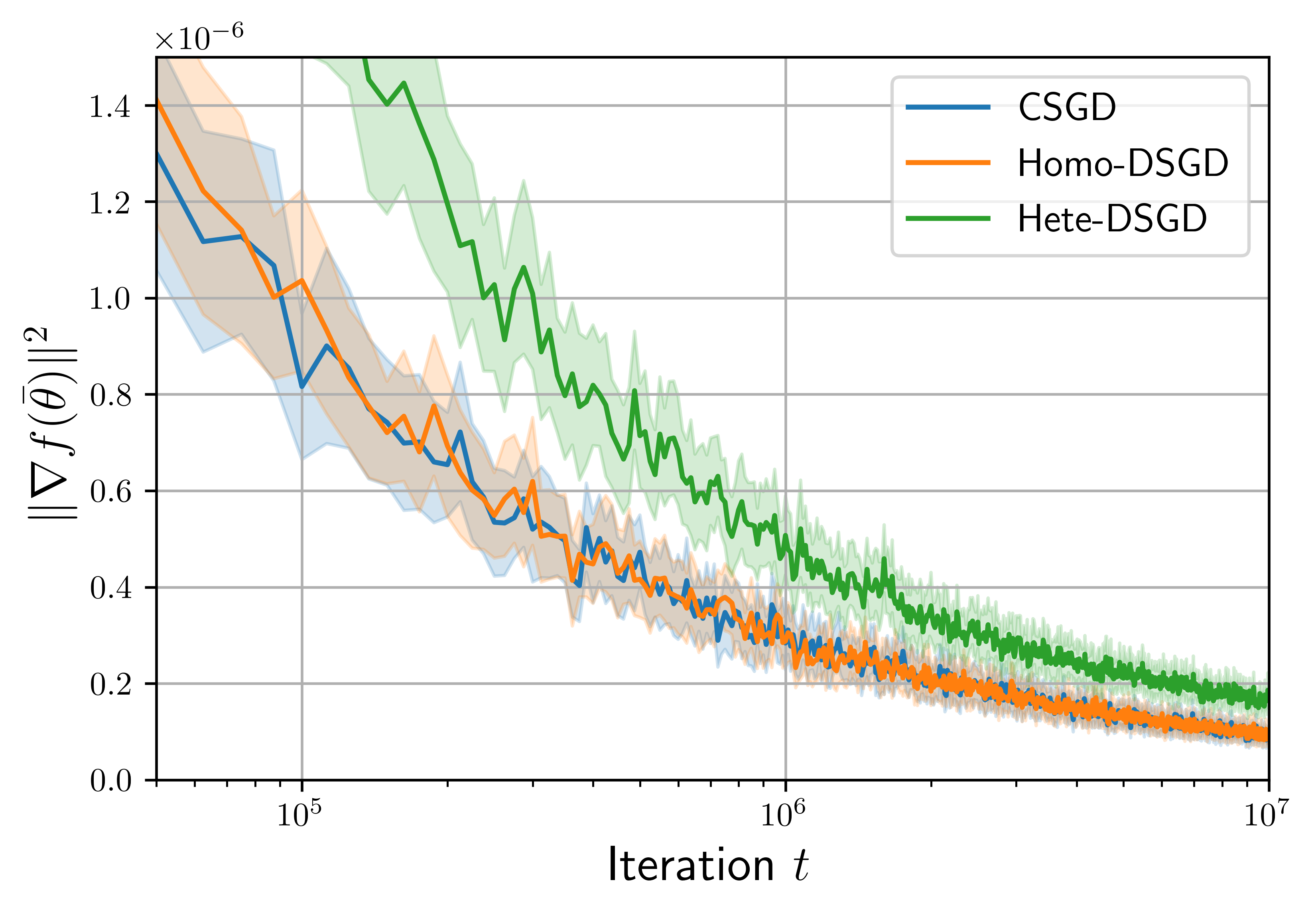
Figure 1: Comparing the convergence behavior of DSGD algorithm under homogeneous / heterogeneous data alongside with CSGD. At each iteration, each agent simulated in the Homo-DSGD/Hete-DSGD algorithms take $1$ sample, while the CSGD algorithm takes a batch of $n$ samples.

Our aim is to verify Theorem 1, 2 via comparing the performance of DSGD under homogeneous and heterogeneous data. Consider a binary classification problem using a linear model for (1), (2), where the loss function takes the form of a non-convex sigmoid function:

$$\textstyle\ell(\bm{\theta};z)=({1+\exp(y\langle x\,|\,\bm{\theta}\rangle)})^{-1}+\frac{\beta}{2}\left\|\bm{\theta}\right\|^{2},$$ (30)

where $z\equiv(x,y)$ with the feature $x\in\mathbb{R}^{d}$, the label $y\in\{\pm 1\}$ represents a (training) data sample and $\beta>0$ is a regularization parameter. Note that (30) satisfies A2–A7. We consider $n=12$ agents connected on a ring graph, with a self weight of $W_{ii}=0.9$.

We set $d=5$ and $\beta=10/m$, where $m$ is the total number of data samples at the agents. To simulate the heterogeneous data setting ($\varsigma,\varsigma_{H}\neq 0$), we first generate the parameter vectors as $\bm{\theta}_{\text{o},i}\in{\cal U}[-1+\frac{i-1}{6},-1+\frac{i}{6}]^{5}$ , $i=1,\ldots,12$. Then, for each $i=1,\ldots,12$, the data distribution ${\sf B}_{i}$ is taken to be the empirical distribution of $n_{i}=200$ samples $\{x_{j}^{i},y_{j}^{i}\}_{j=1}^{200}$, which are generated as

$$x_{j}^{i}\sim{\cal U}[-1,1]^{5},~{}~{}y_{j}^{i}=\mathop{\mathrm{sgn}}(\left\langle x_{j}^{i}\,|\,\bm{\theta}_{\text{o},i}\right\rangle).$$

Subsequently, we denote the algorithm where agent $i$ draws samples from the above ${\sf B}_{i}$ as the Hete-DSGD algorithm. On the other hand, to simulate the homogeneous data setting ($\varsigma,\varsigma_{H}=0$), we consider a combined dataset by taking $\tilde{\sf B}_{i}$ to be the empirical distribution of $\{\{x_{j}^{i},y_{j}^{i}\}_{j=1}^{200}\}_{i=1}^{12}$ such that ${\sf B}=\tilde{\sf B}_{i}$ for all $i$. The corresponding algorithm is denoted as the Homo-DSGD algorithm. As benchmark, we also consider the CSGD algorithm which draws a minibatch of $n=12$ samples from ${\sf B}$ at each iteration. Furthermore, we set the stepsize in the algorithms as $\gamma_{t+1}=\sqrt{a_{0}/(a_{1}+t)}$ with $a_{0}=1/\beta$, $a_{1}=8L^{2}/\beta^{2}$. For the Homo-DSGD/Hete-DSGD algorithms, the initial solution for each agent is randomly drawn as $\bm{\theta}_{i}^{(0)}\sim{\cal N}(1,0.8)^{5}$, and we use the average $\overline{\bm{\theta}}^{(0)}$ as the initial solution for CSGD.

In Fig. 1, we compare the norm of gradient $\|{\nabla}f(\overline{\bm{\theta}}^{t})\|^{2}$ against the number of iteration $t$ for the tested algorithms, over $50$ repeated runs of the stochastic algorithms. The shaded region indicate the 95% confidence interval. Observe that the two DSGD algorithms approach the same steady state convergence behavior as the centralized algorithm CSGD as $t\to\infty$, validating our basic result in Theorem 1. Moreover, we observe that the Homo-DSGD algorithm matches the performance of CSGD with a much smaller transient time than the Hete-DSGD algorithm. The observation corroborates with Theorem 2.

VI Conclusions

In this work, we provided a fine grained analysis for the convergence rate of DSGD while focusing on the role of data homogeneity. Particularly, we show that the plain DSGD algorithm may achieve fast convergence when the data distribution across agents are similar to each other. Our theoretical results are supported by numerical experiment.

Appendix A Proof of Lemma 3

Throughout the appendix, we shall use the notations ${\nabla}f_{i}^{t}:={\nabla}f_{i}(\bm{\theta}_{i}^{t})$, $\tilde{\nabla}f_{i}^{t}:={\nabla}\ell(\bm{\theta}_{i}^{t};z_{i}^{t+1})$, and

$$\tilde{\nabla}F^{t}\mathrel{\mathop{:}}=\left(\tilde{\nabla}f_{1}^{t},\tilde{\nabla}f_{2}^{t},\cdots,\tilde{\nabla}f_{n}^{t}\right)^{\top}\in\mathbb{R}^{n\times d}.$$

Turning our attention back to the proof of Lemma 3. Using A2 and (21), we have

$$f(\overline{\bm{\theta}}^{t+1})\leq f(\overline{\bm{\theta}}^{t})-\langle{\nabla}f(\overline{\bm{\theta}}^{t})|{\textstyle\frac{\gamma_{t+1}}{n}}\!\sum_{i=1}^{n}\!\tilde{\nabla}f_{i}^{t}\rangle+{\textstyle\frac{\gamma_{t+1}^{2}L}{2n^{2}}}\left\|\sum_{i=1}^{n}\tilde{\nabla}f_{i}^{t}\right\|^{2}.$$

Taking the conditional expectation $\mathbb{E}_{t}[\cdot]$ on both sides yields

$$\!\mathbb{E}_{t}[f(\overline{\bm{\theta}}^{t+1})] \leq f(\overline{\bm{\theta}}^{t})\!-\!\gamma_{t+1}\textstyle\left\langle{\nabla}f(\overline{\bm{\theta}}^{t})\,|\,\frac{1}{n}\sum_{i=1}^{n}{\nabla}f_{i}^{t}\right\rangle$$ (31)

$$\textstyle\quad+\gamma_{t+1}^{2}\frac{L}{2}\mathbb{E}_{t}\left[\left\|\frac{1}{n}\sum_{i=1}^{n}\tilde{\nabla}f_{i}^{t}\right\|^{2}\right].$$

We note that the second term is lower bounded by

$$\textstyle\langle{\nabla}f(\overline{\bm{\theta}}^{t})\,|\,\frac{1}{n}\sum_{i=1}^{n}{\nabla}f_{i}^{t}\rangle$$

$$\geq\textstyle\frac{1}{2}\|{\nabla}f(\overline{\bm{\theta}}^{t})\|^{2}-\frac{1}{2}\left\|\frac{1}{n}\sum_{i=1}^{n}\big{(}{\nabla}f_{i}(\overline{\bm{\theta}}^{t})-{\nabla}f_{i}^{t}\big{)}\right\|^{2},$$

and the last term can be upper bounded by

$$\textstyle\mathbb{E}_{t}\left[\left\|\frac{1}{n}\sum_{i=1}^{n}\tilde{\nabla}f_{i}^{t}\right\|^{2}\right]\leq\frac{\sigma^{2}}{n}+\left\|\frac{1}{n}\sum_{i=1}^{n}{\nabla}f_{i}^{t}\right\|^{2}$$

$$\textstyle\leq\frac{\sigma^{2}}{n}+2\|{\nabla}f(\overline{\bm{\theta}}^{t})\|^{2}+2\left\|\frac{1}{n}\sum_{i=1}^{n}\big{(}{\nabla}f_{i}(\overline{\bm{\theta}}^{t})-{\nabla}f_{i}^{t}\big{)}\right\|^{2},$$

where we have used A3 in the first inequality. Substituting into (31) and using the step size condition $\gamma_{t+1}\leq\frac{1}{4L}$ gives

$$\mathbb{E}_{t}[f(\overline{\bm{\theta}}^{t+1})]\leq f(\overline{\bm{\theta}}^{t})-\frac{\gamma_{t+1}}{4}\|{\nabla}f(\overline{\bm{\theta}}^{t})\|^{2}+\frac{\gamma_{t+1}^{2}L\sigma^{2}}{2n}$$ (32)

$$\textstyle+\gamma_{t+1}\left\|\frac{1}{n}\sum_{i=1}^{n}\big{(}{\nabla}f_{i}(\overline{\bm{\theta}}^{t})-{\nabla}f_{i}(\bm{\theta}_{i}^{t})\big{)}\right\|^{2}$$

Observe that by A2, the last term is bounded by:

$$\textstyle\left\|\frac{1}{n}\sum_{i=1}^{n}\big{(}{\nabla}f_{i}(\overline{\bm{\theta}}^{t})-{\nabla}f_{i}^{t}\big{)}\right\|^{2}\leq\frac{L^{2}}{n}\left\|\overline{\bm{\Theta}}^{t}-\bm{\Theta}^{t}\right\|^{2}_{F}.$$

Substituting back into (32) leads to

$$\mathbb{E}_{t}[f(\overline{\bm{\theta}}^{t+1})] \leq f(\overline{\bm{\theta}}^{t})-\frac{\gamma_{t+1}}{4}\|{\nabla}f(\overline{\bm{\theta}}^{t})\|^{2}+\frac{\gamma_{t+1}^{2}L\sigma^{2}}{2n}$$ (33)

$$+\gamma_{t+1}\frac{L^{2}}{n}\left\|\overline{\bm{\Theta}}^{t}-\bm{\Theta}^{t}\right\|^{2}_{F}.$$

This concludes the proof.

Appendix B Proof of Lemma 4

We observe the following chain:

$$\bm{\Theta}^{t+1}-\overline{\bm{\Theta}}^{t+1}=\left({\bm{I}}-\frac{1}{n}{\bm{1}}{\bm{1}}^{\top}\right)\bm{\Theta}^{t+1}={\bm{U}}{\bm{U}}^{\top}\bm{\Theta}^{t+1}$$

$$={\bm{U}}{\bm{U}}^{\top}\left({\bm{W}}\bm{\Theta}^{t}-\gamma_{t+1}\tilde{\nabla}F^{t}\right)$$

$$={\bm{U}}{\bm{U}}^{\top}\left[{\bm{W}}\left({\bm{U}\bm{U}}^{\top}+\frac{1}{n}{\bm{1}\bm{1}}^{\top}\right)\bm{\Theta}^{t}-\gamma_{t+1}\tilde{\nabla}F^{t}\right]$$

$$={\bm{U}}\left({\bm{U}}^{\top}{\bm{W}}{\bm{U}}\right){\bm{U}}^{\top}\bm{\Theta}^{t}-\gamma_{t+1}{\bm{U}}{\bm{U}}^{\top}\tilde{\nabla}F^{t}$$ (34)

Using A1 shows that $\left\|\bm{\Theta}_{o}^{t+1}\right\|_{F}^{2}$ is upper bounded by

$$(1+\alpha)(1-\rho)^{2}\left\|\bm{\Theta}_{o}^{t}\right\|_{F}^{2}\!+\!\left(1+\frac{1}{\alpha}\right)\gamma_{t+1}^{2}\left\|{\bm{U}\bm{U}}^{\top}\tilde{\nabla}F^{t}\right\|_{F}^{2},$$

for any $\alpha>0$. Setting $\alpha=\frac{\rho}{1-\rho}$ gives

$$\left\|\bm{\Theta}_{o}^{t+1}\right\|_{F}^{2} \leq(1-\rho)\left\|\bm{\Theta}_{o}^{t}\right\|_{F}^{2}+\frac{\gamma_{t+1}^{2}}{\rho}\left\|{\bm{U}\bm{U}}^{\top}\tilde{\nabla}F^{t}\right\|_{F}^{2}.$$ (35)

We observe that

$$\left\|{\bm{U}\bm{U}}^{\top}\tilde{\nabla}F^{t}\right\|_{F}^{2}=\sum_{i=1}^{n}\left\|\tilde{\nabla}f_{i}^{t}-\frac{1}{n}\sum_{j=1}^{n}\tilde{\nabla}f_{j}^{t}\right\|^{2}$$

$$\!=\!\sum_{i=1}^{n}\left\|\tilde{\nabla}f_{i}^{t}\!-\!{\nabla}f_{i}^{t}\!+\!{\nabla}f_{i}^{t}\!-\!\frac{1}{n}\sum_{j=1}^{n}{\nabla}f_{j}^{t}\!-\!\frac{1}{n}\sum_{j=1}^{n}\left(\tilde{\nabla}f_{j}^{t}\!-\!{\nabla}f_{j}^{t}\right)\right\|^{2}$$

Taking the conditional expectation $\mathbb{E}_{t}[\cdot]$ yields

$$\mathbb{E}_{t}\left[\left\|{\bm{U}\bm{U}}^{\top}\tilde{\nabla}F^{t}\right\|_{F}^{2}\right]\leq 2n\sigma^{2}+\sum_{i=1}^{n}\left\|{\nabla}f_{i}^{t}-\frac{1}{n}\sum_{j=1}^{n}{\nabla}f_{j}^{t}\right\|^{2}$$

$$\overset{(a)}{\leq}2n(\varsigma^{2}+\sigma^{2})+\frac{2L^{2}}{n}\sum_{i=1}^{n}\sum_{j=1}^{n}\left\|\bm{\theta}_{i}^{t}-\bm{\theta}_{j}^{t}\right\|^{2}$$

$$\leq 2n(\varsigma^{2}+\sigma^{2})+8L^{2}\left\|\bm{\Theta}_{o}^{t}\right\|_{F}^{2}$$

where (a) is obtained by adding and subtracting ${\nabla}f(\bm{\theta}_{i}^{t})$ and using A2, A4. Substituting back into (35) yields

$$\mathbb{E}_{t}[\left\|\bm{\Theta}_{o}^{t+1}\right\|_{F}^{2}]\!\leq\!(1\!-\!\rho+\frac{8L^{2}\gamma_{t+1}^{2}}{\rho})\left\|\bm{\Theta}_{o}^{t}\right\|_{F}^{2}\!+\!\frac{2n\gamma_{t+1}^{2}}{\rho}\left(\varsigma^{2}\!+\!\sigma^{2}\right).$$

Setting $\gamma_{t+1}\leq\frac{\rho}{4L}$ yields that

$$\mathbb{E}[\left\|\bm{\Theta}_{o}^{t+1}\right\|_{F}^{2}]\leq\left(1-\frac{\rho}{2}\right)\mathbb{E}[\left\|\bm{\Theta}_{o}^{t}\right\|_{F}^{2}]+\frac{\gamma_{t+1}^{2}}{\rho}2n\left(\varsigma^{2}+\sigma^{2}\right).$$

Solving the recursion and noticing that $\bm{\Theta}_{o}^{0}={\bm{0}}$ yields

$$\mathbb{E}[\left\|\bm{\Theta}_{o}^{t+1}\right\|_{F}^{2}] \leq\frac{2n(\varsigma^{2}\!+\!\sigma^{2})}{\rho}\sum_{i=1}^{t+1}\gamma_{i}^{2}(1-\frac{\rho}{2})^{t+1-i}$$

$$\leq\frac{8n}{\rho^{2}}\gamma_{t+1}^{2}\left(\varsigma^{2}\!+\!\sigma^{2}\right).$$

where we have applied Lemma 7 in the last inequality.

Appendix C Proof of Lemma 5

We develop the lemma starting from (32) and focus on analyzing the last term therein. Using A5, we observe that:

$$\left\|\frac{1}{n}\sum_{i=1}^{n}\big{(}{\nabla}f_{i}(\overline{\bm{\theta}}^{t})-{\nabla}f_{i}^{t}\big{)}\right\|^{2}=\bigg{\|}\frac{1}{n}\sum_{i=1}^{n}\big{(}{\nabla}f_{i}^{t}-{\nabla}f_{i}(\overline{\bm{\theta}}^{t})$$

$$\qquad-{\nabla}^{2}f_{i}(\overline{\bm{\theta}}^{t})(\bm{\theta}_{i}^{t}-\overline{\bm{\theta}}^{t})+{\nabla}^{2}f_{i}(\overline{\bm{\theta}}^{t})(\bm{\theta}_{i}^{t}-\overline{\bm{\theta}}^{t})\big{)}\bigg{\|}^{2}$$

$$\leq 2\left\|\frac{1}{n}\sum_{i=1}^{n}\big{(}{\nabla}f_{i}^{t}-{\nabla}f_{i}(\overline{\bm{\theta}}^{t})-{\nabla}^{2}f_{i}(\overline{\bm{\theta}}^{t})(\bm{\theta}_{i}^{t}-\overline{\bm{\theta}}^{t})\big{)}\right\|^{2}$$

$$\qquad+2\left\|\frac{1}{n}\sum_{i=1}^{n}{\nabla}^{2}f_{i}(\overline{\bm{\theta}}^{t})(\bm{\theta}_{i}^{t}-\overline{\bm{\theta}}^{t})\right\|^{2}$$

$$\leq\frac{L_{H}^{2}}{2n}\,\|\bm{\Theta}^{t}-\overline{\bm{\Theta}}^{t}\|_{F}^{4}+\frac{2}{n^{2}}\left\|\sum_{i=1}^{n}{\nabla}^{2}f_{i}(\overline{\bm{\theta}}^{t})(\bm{\theta}_{i}^{t}-\overline{\bm{\theta}}^{t})\right\|^{2},$$

where the last inequality is due to A5 and (26). Furthermore, by A6, we obtain

$$\quad\!\bigg{\|}\!\sum_{i=1}^{n}{\nabla}^{2}f_{i}(\overline{\bm{\theta}}^{t})(\bm{\theta}_{i}^{t}-\overline{\bm{\theta}}^{t})\bigg{\|}^{2}$$

$$\!\overset{(a)}{=}\!\left\|\sum_{i=1}^{n}({\nabla}^{2}f_{i}(\overline{\bm{\theta}}^{t})\!-\!{\nabla}^{2}f(\overline{\bm{\theta}}^{t}))(\bm{\theta}_{i}^{t}\!-\!\overline{\bm{\theta}}^{t})\right\|^{2}\!\leq\!n\varsigma_{H}^{2}\|\bm{\Theta}^{t}\!-\!\overline{\bm{\Theta}}^{t}\|_{F}^{2},$$

where (a) is due to $\sum_{i=1}^{n}{\nabla}^{2}f(\overline{\bm{\theta}}^{t})(\bm{\theta}_{i}^{t}-\overline{\bm{\theta}}^{t})={\bm{0}}$. This yields

$$\left\|\frac{1}{n}\sum_{i=1}^{n}\big{(}{\nabla}f_{i}(\overline{\bm{\theta}}^{t})-{\nabla}f_{i}(\bm{\theta}_{i}^{t})\big{)}\right\|^{2}$$

$$\leq\frac{1}{n}\left(\frac{L_{H}^{2}}{2}\|\bm{\Theta}^{t}-\overline{\bm{\Theta}}^{t}\|_{F}^{2}+\varsigma_{H}^{2}\right)\|\bm{\Theta}^{t}\!-\!\overline{\bm{\Theta}}^{t}\|_{F}^{2}.$$

Substituting back into (31) leads to

$$\begin{aligned} &\mathbb{E}_{t}[f(\overline{\bm{\theta}}^{t+1})]\leq f(\overline{\bm{\theta}}^{t})-\frac{\gamma_{t+1}}{4}\|{\nabla}f(\overline{\bm{\theta}}^{t})\|^{2}+\frac{\gamma_{t+1}^{2}L\sigma^{2}}{2n}\\ &\qquad+\frac{\gamma_{t+1}}{2n}\Big{(}L_{H}^{2}\|\bm{\Theta}^{t}-\overline{\bm{\Theta}}^{t}\|_{F}^{2}+2\varsigma_{H}^{2}\Big{)}\|\bm{\Theta}^{t}-\overline{\bm{\Theta}}^{t}\|_{F}^{2}.\end{aligned}$$

This concludes the proof.

Appendix D Proof of Lemma 6

Similar to the proof of Lemma 4, using A1 and (34), the following holds for any $\alpha,\beta>0$,

$$\left\|\bm{\Theta}_{o}^{t+1}\right\|^{4}_{F} \leq\bigg{[}(1+\alpha)(1-\rho)^{2}\left\|{\bm{U}\bm{U}}^{\top}\bm{\Theta}^{t}\right\|_{F}^{2}$$

$$\quad\textstyle+\left(1+\frac{1}{\alpha}\right)\gamma_{t+1}^{2}\left\|{\bm{U}\bm{U}}^{\top}\tilde{\nabla}F^{t}\right\|_{F}^{2}\bigg{]}^{2}$$

$$\leq(1+\beta)(1+\alpha)^{2}(1-\rho)^{4}\cdot\left\|\bm{\Theta}_{o}^{t}\right\|_{F}^{4}$$

$$\quad\textstyle+(1+\frac{1}{\beta})(1+\frac{1}{\alpha})^{2}\gamma_{t+1}^{4}\left\|{\bm{U}}{\bm{U}}^{\top}\tilde{\nabla}F^{t}\right\|^{4}_{F}.$$

Setting $\alpha=\beta=\frac{\rho}{1-\rho}$, then $1+1/\alpha=1+1/\beta=1/\rho$, which leads to the following

$$\left\|\bm{\Theta}_{o}^{t+1}\right\|^{4}_{F}\leq(1-\rho)\left\|\bm{\Theta}_{o}^{t}\right\|_{F}^{4}+\frac{\gamma_{t+1}^{4}}{\rho^{3}}\left\|{\bm{U}}{\bm{U}}^{\top}\tilde{\nabla}F^{t}\right\|_{F}^{4}.$$ (36)

The second term can be expanded as:

$$\left\|{\bm{U}}{\bm{U}}^{\top}\tilde{\nabla}F^{t}\right\|_{F}^{4}=\left(\sum_{i=1}^{n}\left\|\tilde{\nabla}f_{i}^{t}-\frac{1}{n}\sum_{j=1}^{n}\tilde{\nabla}f_{j}^{t}\right\|^{2}\right)^{2}.$$

Adding and subtracting ${\nabla}f_{i}^{t},\frac{1}{n}\sum_{j=1}^{n}{\nabla}f_{j}^{t}$ leads to the upper bound:

$$\left\|{\bm{U}}{\bm{U}}^{\top}\tilde{\nabla}F^{t}\right\|_{F}^{4} \leq\textstyle 27n\sum_{i=1}^{n}\Bigg{[}\left\|\frac{1}{n}\sum_{j=1}^{n}(\tilde{\nabla}f_{j}^{t}-{\nabla}f_{j}^{t})\right\|^{4}$$

$$\textstyle+\left\|\tilde{\nabla}f_{i}^{t}-{\nabla}_{i}^{t}\right\|^{4}+\left\|{\nabla}f_{i}^{t}-\frac{1}{n}\sum_{j=1}^{n}{\nabla}f_{j}^{t}\right\|^{4}\Bigg{]},$$

where we have used $(a+b+c)^{4}\leq 27(a^{4}+b^{4}+c^{4})$. Using the Cauchy-Schwarz inequality, we bound the last term in the above inequality as:

$$\left\|\frac{1}{n}\sum_{j=1}^{n}(\tilde{\nabla}f_{j}^{t}\!-\!{\nabla}f_{j}^{t})\right\|^{4} \leq\frac{1}{n^{4}}\left(n\sum_{j=1}^{n}\left\|\tilde{\nabla}f_{j}^{t}-{\nabla}f_{j}^{t}\right\|^{2}\right)^{2}$$

$$\leq\frac{1}{n}\sum_{j=1}^{n}\left\|\tilde{\nabla}f_{j}^{t}-{\nabla}f_{j}^{t}\right\|^{4}$$

By A7, we observe that

$$\mathbb{E}_{t}\left\|{\bm{U}}{\bm{U}}^{\top}\tilde{\nabla}F^{t}\right\|_{F}^{4}\leq 27n\sum_{i=1}^{n}\bigg{[}2\sigma^{4}+\left\|{\nabla}f_{i}^{t}-\frac{1}{n}\sum_{j=1}^{n}{\nabla}f_{j}^{t}\right\|^{4}\bigg{]}$$

Adding and subtracting ${\nabla}f(\bm{\theta}_{i}^{t})=\frac{1}{n}\sum_{j=1}^{n}{\nabla}f_{j}(\bm{\theta}_{i}^{t})$ in the last term leads to

$$\mathbb{E}_{t}\left\|{\bm{U}}{\bm{U}}^{\top}\tilde{\nabla}F^{t}\right\|_{F}^{4} \leq 27n\bigg{\{}2n\sigma^{2}+8\sum_{i=1}^{n}\left\|{\nabla}f_{i}^{t}\!-\!{\nabla}f(\bm{\theta}_{i}^{t})\right\|^{4}\!$$

$$\quad+\textstyle 8\sum_{i=1}^{n}\left\|\frac{1}{n}\sum_{j=1}^{n}{\nabla}f_{j}(\bm{\theta}_{i}^{t})\!-\!{\nabla}f_{j}^{t})\right\|^{4}\bigg{\}}$$

Applying A2, A4 yields

$$\!\mathbb{E}_{t}\left\|{\bm{U}}{\bm{U}}^{\top}\tilde{\nabla}F^{t}\right\|_{F}^{4}\!\leq\!27n\!\left\{\!2n\sigma^{4}\!+\!8n\varsigma^{4}+\frac{8L^{4}}{n}\!{\sum_{i,j=1}^{n}\!}\left\|\bm{\theta}_{i}^{t}-\bm{\theta}_{j}^{t}\right\|^{4}\!\right\}\!.$$

Observe that the last terms are upper bounded by the consensus error $2\left\|\overline{\bm{\Theta}}^{t}-\bm{\Theta}^{t}\right\|^{4}$. We obtain:

$$\mathbb{E}_{t}\left\|{\bm{U}}{\bm{U}}^{\top}\tilde{\nabla}F^{t}\right\|_{F}^{4} \leq 54n^{2}\Bigg{\{}\sigma^{4}\!+\!4\varsigma^{4}\!+\!\frac{64L^{4}}{n^{2}}\left\|\overline{\bm{\Theta}}^{t}-\bm{\Theta}^{t}\right\|_{F}^{4}\!\Bigg{\}}.$$

Substituting the upper bound of $\left\|{\bm{U}}{\bm{U}}^{\top}\tilde{\nabla}F^{t}\right\|_{F}^{4}$ to inequality (36), we have that

$$\mathbb{E}\left\|\bm{\Theta}_{o}^{t+1}\right\|^{4}_{F} \leq\left(1-\rho+\frac{\gamma_{t+1}^{4}}{\rho^{3}}3456L^{4}\right)\mathbb{E}\left\|\bm{\Theta}_{o}^{t}\right\|_{F}^{4}$$

$$\quad+54n^{2}(\sigma^{4}+4\varsigma^{4})\frac{\gamma_{t+1}^{4}}{\rho^{3}}$$

With the stepsize condition $\gamma_{t+1}\leq\frac{\rho}{9L}$, we obtain

$$\mathbb{E}\left\|\bm{\Theta}_{o}^{t+1}\right\|^{4}_{F} \leq\left(1-\frac{\rho}{2}\right)\mathbb{E}\left\|\bm{\Theta}_{o}^{t}\right\|_{F}^{4}+54n^{2}(\sigma^{4}+4\varsigma^{4})\frac{\gamma_{t+1}^{4}}{\rho^{3}}.$$

Solving the recursion and noticing that $\bm{\theta}_{i}^{0}=\bm{\theta}_{j}^{0}$ give

$$\mathbb{E}\left\|\bm{\Theta}_{o}^{t+1}\right\|^{4}_{F}\leq\frac{54n^{2}(\sigma^{4}\!+\!4\varsigma^{4})}{\rho^{3}}\sum_{j=1}^{t+1}\gamma_{j}^{4}\left(1-\frac{\rho}{2}\right)^{t+1-j}$$

Applying Lemma 7, we have

$$\mathbb{E}\left\|\bm{\Theta}_{o}^{t+1}\right\|^{4}_{F}\leq\frac{216(\sigma^{4}+4\varsigma^{4})n^{2}}{\rho^{4}}\gamma_{t+1}^{4}.$$

This concludes the proof.

Appendix E An Auxiliary Lemma

Lemma 7.

Let $\{\gamma_{t}\}_{t\geq 1}$ be an arbitrary sequence of non-negative number and let $b\in\mathbb{R}^{+}$ be given,

• If $\frac{\gamma_{t}^{2}}{\gamma_{t+1}^{2}}\leq 1+b\gamma_{t+1}^{2}$, $\forall t$, and $\sup_{t\geq 1}\gamma_{t}\leq\sqrt{\frac{\rho/4}{b(1-\rho/2)}}$. The following holds:

  $$\sum_{i=1}^{t+1}\gamma_{i}^{2}(1-\frac{\rho}{2})^{t+1-i}\leq\frac{4}{\rho}\gamma_{t+1}^{2}$$ (37)

• If $\frac{\gamma_{t}^{4}}{\gamma_{t+1}^{4}}\leq 1+b\gamma_{t+1}^{4}$, $\forall t$, and $\sup_{t\geq 1}\gamma_{t}\leq\sqrt[4]{\frac{\rho/4}{b(1-\rho/2)}}$. The following holds:

  $$\sum_{i=1}^{t+1}\gamma_{i}^{4}(1-\frac{\rho}{2})^{t+1-i}\leq\frac{4}{\rho}\gamma_{t+1}^{4}$$ (38)

Proof.

Observe the following chain:

$$\begin{aligned} &\sum_{i=1}^{t+1}\gamma_{i}^{2}(1-\frac{\rho}{2})^{t+1-i}\\ &\leq\sum_{i=1}^{n}\frac{\gamma_{i}^{2}}{\gamma_{i+1}^{2}}\cdot\frac{\gamma_{i+1}^{2}}{\gamma_{i+2}^{2}}\cdot\frac{\gamma_{t}^{2}}{\gamma_{t+1}^{2}}\cdot\gamma_{t+1}^{2}(1-\frac{\rho}{2})^{t+1-i}\\ &\leq\gamma_{t+1}^{2}\sum_{i=1}^{t+1}\left[(1+b\gamma_{i+1}^{2})(1-\frac{\rho}{2})\right]^{t+1-i}\\ &\leq\gamma_{t+1}^{2}\sum_{i=1}^{t+1}(1-\frac{\rho}{4})^{t+1-i}\leq\frac{4\gamma_{t+1}^{2}}{\rho}\end{aligned}$$

where the last inequality is due to the condition $\gamma_{i+1}\leq\sqrt{\frac{\rho/4}{b(1-\rho/2)}}$. This concludes the proof for (37).

For the fourth order case in (38), we omit the proof due to space limitation. Notice that it follows directly from the above derivation on the second order case. ∎

References

- [1] A. Nedic and A. Ozdaglar, “Distributed subgradient methods for multi-agent optimization,” IEEE Transactions on Automatic Control, vol. 54, no. 1, pp. 48–61, 2009.
- [2] L. Bottou, F. E. Curtis, and J. Nocedal, “Optimization methods for large-scale machine learning,” SIAM Review, 2018.
- [3] T.-H. Chang, M. Hong, H.-T. Wai, X. Zhang, and S. Lu, “Distributed learning in the nonconvex world: From batch data to streaming and beyond,” IEEE Signal Processing Magazine, vol. 37, no. 3, 2020.
- [4] Y. Zhang and L. Xiao, “Communication-efficient distributed optimization of self-concordant empirical loss,” in Large-Scale and Distributed Optimization. Springer, 2018, pp. 289–341.
- [5] S. J. Reddi, J. Konecný, P. Richtárik, B. Póczos, and A. Smola, “Aide: Fast and communication efficient distributed optimization,” arXiv preprint arXiv:1608.06879, 2016.
- [6] J. Wang, Z. Charles, Z. Xu, G. Joshi, H. B. McMahan, M. Al-Shedivat, G. Andrew, S. Avestimehr, K. Daly, D. Data et al., “A field guide to federated optimization,” arXiv preprint arXiv:2107.06917, 2021.
- [7] S. Sundhar Ram, A. Nedić, and V. V. Veeravalli, “Distributed stochastic subgradient projection algorithms for convex optimization,” JOTA, vol. 147, no. 3, pp. 516–545, 2010.
- [8] X. Lian, C. Zhang, H. Zhang, C.-J. Hsieh, W. Zhang, and J. Liu, “Can decentralized algorithms outperform centralized algorithms? a case study for decentralized parallel stochastic gradient descent,” in NeurIPS, 2017.
- [9] S. Pu, A. Olshevsky, and I. C. Paschalidis, “A sharp estimate on the transient time of distributed stochastic gradient descent,” Ieee Transactions On Automatic Control, 2021.
- [10] D. Aldous and J. Fill, Reversible Markov chains and random walks on graphs. Berkeley, 1995.
- [11] C. A. Uribe, S. Lee, A. Gasnikov, and A. Nedić, “A dual approach for optimal algorithms in distributed optimization over networks,” Optimization Methods and Software, vol. 36, no. 1, pp. 171–210, 2021.
- [12] K. Scaman, F. Bach, S. Bubeck, Y. T. Lee, and L. Massoulié, “Optimal algorithms for smooth and strongly convex distributed optimization in networks,” in ICML, 2017, pp. 3027–3036.
- [13] H. Sun, S. Lu, and M. Hong, “Improving the sample and communication complexity for decentralized non-convex optimization: Joint gradient estimation and tracking,” in ICML, 2020, pp. 9217–9228.
- [14] R. Xin, U. Khan, and S. Kar, “A hybrid variance-reduced method for decentralized stochastic non-convex optimization,” in ICML, 2021.
- [15] K. Huang and S. Pu, “Improving the transient times for distributed stochastic gradient methods,” arXiv preprint arXiv:2105.04851, 2021.
- [16] W. Shi, Q. Ling, G. Wu, and W. Yin, “Extra: An exact first-order algorithm for decentralized consensus optimization,” SIAM Journal on Optimization, vol. 25, no. 2, pp. 944–966, 2015.
- [17] P. Frasca, R. Carli, F. Fagnani, and S. Zampieri, “Average consensus on networks with quantized communication,” International Journal of Robust and Nonlinear Control, vol. 19, no. 16, pp. 1787–1816, 2009.
- [18] A. Koloskova, T. Lin, S. U. Stich, and M. Jaggi, “Decentralized deep learning with arbitrary communication compression,” in ICLR, 2019.
- [19] M. Assran, N. Loizou, N. Ballas, and M. Rabbat, “Stochastic gradient push for distributed deep learning,” in ICML, 2019, pp. 344–353.
- [20] S. Vlaski and A. H. Sayed, “Distributed learning in non-convex environments—part i: Agreement at a linear rate,” IEEE Transactions on Signal Processing, vol. 69, pp. 1242–1256, 2021.
- [21] S. Ghadimi and G. Lan, “Stochastic first-and zeroth-order methods for nonconvex stochastic programming,” SIAM Journal on Optimization, vol. 23, no. 4, pp. 2341–2368, 2013.
- [22] Y. Arjevani and O. Shamir, “Communication complexity of distributed convex learning and optimization,” NeurIPS, vol. 28, 2015.
- [23] Y. Tian, G. Scutari, T. Cao, and A. Gasnikov, “Acceleration in distributed optimization under similarity,” in AISTATS, 2022.
- [24] Y. Nesterov, Introductory lectures on convex optimization: A basic course. Springer Science & Business Media, 2003, vol. 87.