Detecting the relative phase between different frequency components of a photon using a three-level atom coupled to a waveguide
Abstract
We study the scattering inside a waveguide of a single photon with a single three-level atom, both of which are in a superposition state. The photon is in a superposition state of two frequencies, whereas the atoms is in a superposition state of two non-degenerate ground states. We find that the scattering depends on both the relative phase between the photon frequencies and the relative phase between the atomic ground states. Our results show that a three-level atom coupled to a waveguide can be used as photon phase filter that could detect the relative phase between the two frequencies of the photon superposition state.
I Introduction
There have been many studies on the generation Zakka-Bajjani et al. (2011); Clemmen et al. (2016); Aguayo-Alvarado et al. (2022) or manipulation Tanzilli et al. (2005); Karnieli and Arie (2018); Lukens and Lougovski (2017); Lu et al. (2020, 2019, 2018); Olislager et al. (2010) of a single photon in a superposition of two frequencies (or ‘colours’). These frequency-superposition states have been called ‘color qubits’ Aguayo-Alvarado et al. (2022), bichromatic photons Clemmen et al. (2016), or frequency-bin qubits Lukens and Lougovski (2017). Such states can be generated in the process of quantum frequency conversion, where a photon’s frequency is converted while its quantum information is maintained, as experimentally demonstrated three decades ago Huang and Kumar (1992). These states also arise in quantum frequency mixing (where different superposition states are converted to and from each other) which has been demonstrated using nonlinearities Kobayashi et al. (2016, 2017), nonlinearities McGuinness et al. (2010); Clemmen et al. (2016); Dmitriev et al. (2017) as well as electro-optic modulation Lu et al. (2018, 2020).
The manipulation of frequency superposition states at the single-photon level has generated interest for its potential applications in quantum information processing Lukens and Lougovski (2017). Building on the work in linear optical quantum computation Knill et al. (2001), frequency-bin qubits have been proposed as an alternative to other photonic qubits such as those based on polarization. Polarization-based qubits can only have a two-dimensional Hilbert space, whereas frequency qubits can have a Hilbert space with much higher dimension. Frequency qubits may also be scalable for on-chip photonics Javid et al. (2021). In recent years, it has been theoretically proposed and experimentally verified that it is possible to achieve arbitrary single-qubit gates in frequency space Lu et al. (2020, 2019). Aside from quantum information processing applications, frequency superposition states may also be useful for quantum metrology Giovannetti et al. (2011) or phase-spectroscopy Rinehart et al. (2012) at the low-light level.
Although the generation and manipulation of single-photon frequency superposition states has been well-studied Yesharim et al. (2022); Zakka-Bajjani et al. (2011); Clemmen et al. (2016); Aguayo-Alvarado et al. (2022); Tanzilli et al. (2005); Karnieli and Arie (2018); Lukens and Lougovski (2017); Lu et al. (2020, 2019, 2018); Olislager et al. (2010), there is less attention devoted to the measurement of the relative phase between different frequency components of such states. Most existing works focus on measuring the amplitude spectrum of the state, where the phase information is lost. The relative phase of two frequency components of a single photon was measured in Ref. Clemmen et al. (2016) using single-photon Ramsey interference. Here, they generated arbitrary frequency-superposition states using Bragg scattering four-wave mixing which is a nonlinear process. The relative phase between different frequency components could be measured because the outcome of their projective measurement depends on this relative phase. A related study uses electro-optic modulators instead of nonlinear processes Lu et al. (2020). Their set-up also allows them to achieve arbitrary frequency qubit rotations on the Bloch sphere and the output state can then be measured using quantum state tomography, where the relative phase between frequency components can be determined using Pauli measurements.
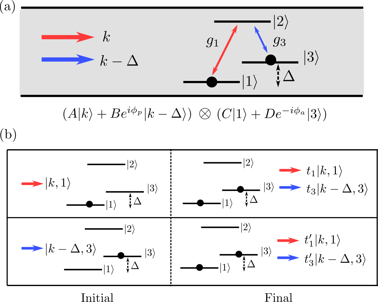
In this study, we propose a novel way to measure the relative phase of different frequency components of a single photon using a setup in waveguide quantum electrodynamics Sheremet et al. (2023); Roy et al. (2017); Türschmann et al. (2019); Chang et al. (2018). Our proposed set-up consists of a three-level atom coupled to a one-dimensional waveguide as seen in Fig. 1(a). The atom is of the type with a two-dimensional ground state manifold spanned by eigenstates and at energy and , respectively, and an excited state at energy . It has been shown that one can prepare the atom to be in an arbitrary ground state in this two-dimensional manifold Djotyan et al. (2008); He et al. (2009); Randall et al. (2018). Here we scatter a single-photon with two frequency components near and (where ) against the atom. We show that with a suitable choice of the atomic ground state, the outcome of the scattering process can be used to determine the relative phase of the two photon frequency components.
Scattering for a atom in a superposition of ground states was studied in Ref. Martens et al. (2013). Quantum state transfer Chan et al. (2022) and quantum frequency conversion Bradford and Shen (2012) has also been studied in a -type atom. However, none of these studies specifically study the dependence of the relative photon phase on the transport for a atom coupled to a waveguide, which is the focus of this work. While the measurement of the relative photon phase of two frequency superposition states was done in EOM Lu et al. (2020) and Ramsey interference setups Clemmen et al. (2016), the benefit of using our setup over these methods, is that our waveguide quantum electrodynamics system can compare the quantum information of two objects. That it is, the scattering output of our system can allow us to measure both the relative phase of the frequency superposition states as well as the relative phase of the atomic ground states in the same platform, as opposed to just one of these phases as in Ref. Lu et al. (2020); Clemmen et al. (2016).
II Model
To treat the system of Fig. 1(a), we use a real space formalism originally developed in Ref. Shen and Fan (2005) and applied to three level atoms in Ref. Witthaut and Sørensen (2010). Let be the atom-photon coupling constants for the and transitions and assume the transition is forbidden. The Hamiltonian for this system is given by Shen and Fan (2007); Roy et al. (2017); Shen and Fan (2005); Bradford and Shen (2012); Witthaut and Sørensen (2010):
| (1) |
where
| (2) | ||||
are the photonic, atomic and interaction terms of the Hamiltonian respectively. In this paper we set . Here, is the group velocity of the photons travelling in the waveguide, and are the creation operators for a right-going and left-going photon at position in the waveguide. We have chosen to linearize the dispersion relation of the waveguide around the frequency . The Hamiltonian of Eq. (1) describes a three-level atom coupled to a single-mode waveguide. In a three-level atom, the two transitions may couple to different polarizations. For a single-mode waveguide however, as long as the waveguide mode has non-zero components in both polarizations, the waveguide mode will couple to both transitions and our theory will be applicable. Moreover, there are experimental platforms of three level atoms such as in superconducting qubits Schuster et al. (2005) or quantum dots Manga Rao and Hughes (2007), where these three-level system can be designed to couple with a single-mode waveguide.
The total excitation number operator commutes with the Hamiltonian . The basis states corresponding to the eigenstates of the number operator in the single-excitation regime are:
| (3) |
Since , we also use these basis states in Eq. (3) to expand the scattering eigenstate of the Hamiltonian with a total energy in the single-excitation regime as Shen and Fan (2005):
| (4) |
Here the ’s are the single-photon field amplitudes. The subscripts of denotes whether the photon is right or left-going, and the state of the atom. For example describes the case where the photon is right-going, and the atom is in state . is the probability amplitude of the three-level atom being in the excited state. is a vacuum state with zero photons and the atom is in state . Using Eq. (4) and Eq. (1) with the time-independent Schrodinger equation gives the following set of linear differential equations:
| (5) | ||||
| (6) | ||||
| (7) | ||||
| (8) | ||||
| (9) |
We first consider a scenario where the atom is initially in the state and a right-going photon is incoming from the left. Our photon wave-function ansatz is:
| (10) | |||
| (11) | |||
| (12) | |||
| (13) |
() gives the probability that a photon will be transmitted (reflected) leaving the atom in the or state respectively when the atom was initially in . Here, is the Heaviside function with . Using our ansatz and Eq. (5) with and Eq. (7) with , we find that , and . Substituting these photon wave-functions into Eq. (5) to (9) gives as well as the following solutions:
| (14) | ||||
| (15) | ||||
| (16) | ||||
| (17) | ||||
| (18) |
Here are the decay rates of the state into state and state respectively Rephaeli and Fan (2012); Witthaut and Sørensen (2010).
In the second scenario, we consider the case where the atom is initially in the state and a right-going photon incoming from the left. Our photon wave-function ansatz is
| (19) | |||
| (20) | |||
| (21) | |||
| (22) |
() gives the probability that a photon will be transmitted (reflected) leaving the atom in the or state respectively when the atom was initially in . We can obtain our solutions by substituting this ansatz into the linear differential equations in Eq. (5) to (9) or by simply replacing the labels (due to parity symmetry Shen and Fan (2009)) in Eq. (14) to Eq. (18).
| (23) | ||||
| (24) | ||||
| (25) | ||||
| (26) | ||||
| (27) |
We can now summarize the scattering process for a right-going photon of energy interacting with a atom initially in the state:
| (28) |
where , and the label inside the ket denotes a plane wave of the form . Similarly, for a right-going photon of energy interacting with a atom initially in the state:
| (29) |
The scattering processes for both cases are shown in Fig. 1(b). We note that there are two transmission and reflection output channels for both scenarios.
III Results
Let us now consider a separable input state where the photon is in a superposition state which is a frequency superposition state with two frequencies and and the atom is in a superposition state of the two ground states . With our choice of the two frequencies are on resonance with the two atomic transitions when . are assumed to be real without any loss of generality. is the relative phase between the atomic states and is the relative phase between the two photon frequencies. Our input state is then made of the tensor product of the photon state and the atomic state :
| (30) | ||||
as depicted in Fig. 1(a). The energies of the four components in Eq. (30) are , , and respectively. However, with the choice of the two photon frequencies as described above, the and components in the input state have the same energy .
Applying the scattering processes in Eq. (28) and (29) to each of the four terms in Eq. (30) gives an output state with twelve different terms that have the following probabilities:
| (31) | ||||
| (32) | ||||
| (33) | ||||
| (34) | ||||
| (35) | ||||
| (36) | ||||
| (37) | ||||
| (38) | ||||
| (39) | ||||
| (40) | ||||
| (41) | ||||
| (42) |
The subscript of refers to the outgoing states. For example corresponds to the probability of . Here, . The main result of this paper is that when the input photon frequency states match the atomic resonance levels, both the and input terms can result in the output term. Interference between these two channels causes a dependence of the scattering output on the relative phase . A similar logic applies to the output state. Thus, our scattering output can allow us to compare the effects of both and in the same platform. This is the advantage of our set-up as this phase information is normally lost when it is squared in intensity measurements. The probability amplitudes in Eq. (31) to (34) can be measured by a joint projective measurements on any of the or states. Experimentally, the measurement of the photon state can be carried out with a spectrometer Hempel et al. (2013); Reim et al. (2011). The measurement of the atomic state can then be carried out by scattering a weak classical beam of light against the atom, and by measuring the resulting extinction coefficient Chen et al. (2008); Hwang et al. (2009).
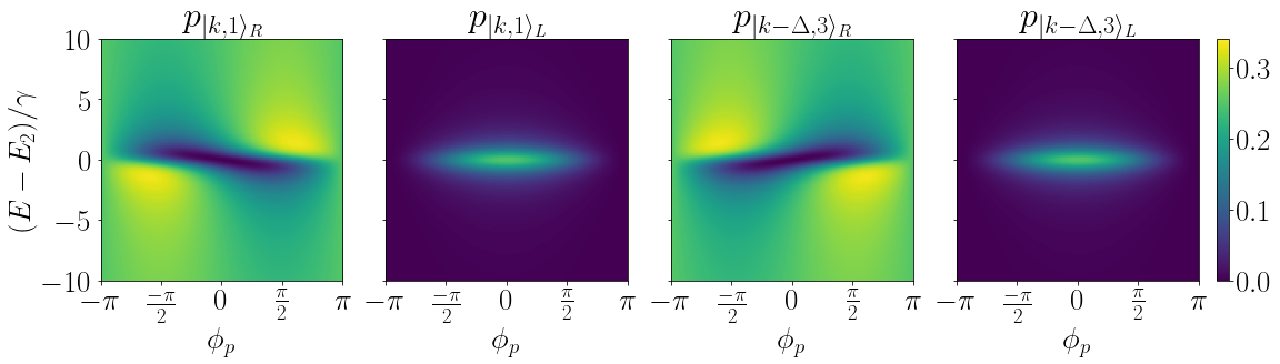
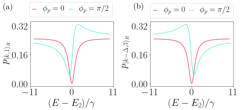
Since the total energy is conserved for each term after scattering, we focus only on the subspace with energy . In Fig. 2, we plot the various probabilities in Eq. (31) to (34) as a function of the normalized total energy and the input photon phase . In Fig. 3, we plot a cross-section from Fig. 2 at for the two transmission terms Eq. (31) and Eq. (33) to highlight the dependence. Here,
| (43) | ||||
Note that we have picked but that changing the initial only results in a phase shift of the results in Eq. (31) to Eq. (34) (shifting the plots in Fig. 2 left or right). Experimentally, a three-level atom can be prepared in a superposition with control over the phase in processes such as fractional stimulated Raman adiabatic passage Vitanov et al. (1999). The sum of the panels in Fig. 2 do not add to 1 because the non-interference terms must also be included. We see that the reflection terms are symmetric about while the transmission terms are asymmetric about . This can be understood by decomposing the input photon state into the scattering mode that maximally excites the atom and the non-scattering mode that does not excite the atom. For arbitrary ( and are constrained to be and ), and in the sub-space with energy , we can solve for the non-scattering mode by setting the total excitation probability to be zero:
| (44) |
from which one obtains
| (45) |
For our parameter set in Eq. (43), this becomes . Hence, the non-scattering mode is
| (46) |
Applying the scattering transformations in Eq. (28) and Eq. (29) to gives back the same state:
| (47) |
We see that the non-scattering mode has no contribution to the reflection, and its transmission has no frequency dependence. The scattering mode is orthogonal to the non-scattering mode, so for this parameter set in Eq. (43), it corresponds to when and can be written as
| (48) |
The scattering output of is
| (49) |
We see that the transmission coefficient of is a constant minus a Lorentzian and the reflection is a Lorentzian.
In the subspace with the energy , any arbitrary input state can be decomposed into a linear superposition of and , as they also form a basis of the Hilbert space for an incoming right-going photon. In this parameter set of Eq. (43) when , the contribution is only from . Thus, the transmission is symmetric about , and the reflection is a Lorentzian as expected from Eq. (49). As does not contribute to the reflection, the reflection remains a Lorentzian for all . On the other hand when , the transmission has components from both and . The interference of the transmission from the scattering mode and the transmission from the non-scattering mode gives rise to a Fano-lineshape Fan and Joannopoulos (2002). This explains the asymmetric transmission about for . The antisymmetry about for the transmission plots in Fig. 2 is because changing the sign of changes the sign of contribution from .
We note that the existence of a non-scattering input mode that does not excite the atom can be alternatively argued as follows: The atomic excitation is a linear function of the amplitudes in the states of and . Therefore, there is always a particular choice of the amplitudes for which .
IV Conclusion
In summary, we have shown that the scattering of a single photon in a superposition of two photon frequencies with a atom in a superposition of two non-degenerate ground states depends on the initial photon phase between the two photon frequencies (and the initial atomic phase between the ground states). Our results show that three-level atoms can be used as a relative photon phase detector for single photons in a superposition state, offering a simpler alternative to other experimental platforms using nonlinear optics Clemmen et al. (2016) and electro-optic modulators Lu et al. (2020). It also allows us to compare the relative phases of two different objects containing quantum information (the relative phase of the frequency superposition states and the relative phase of the atomic ground states) in the same platform. As applications of quantum information increases, it is of practical relevance to have a platform that can compare the effects of both these phases. Furthermore, as waveguide quantum electrodynamics has a wide range of experimental realizations including superconducting qubits, quantum dots, and cold atoms, the theoretical result in this paper may also allow for more versatility and tunability to make this relative photon phase measurement.
Acknowledgements
This work is supported by a Vannevar Bush Faculty Fellowship from the U. S. Department of Defense (Grant No. N00014-17-1-3030). JZ acknowledges A. Poddubny for useful comments.
Appendix: Effect of dephasing or other losses
Various environmental factors such as random fluctuations in the magnetic or electric field, interactions with other particles or quasiparticles or or other defects and coupling with other electromagnetic modes can result in a loss of coherence and hence a decrease in the visibility of transmission or reflectance spectra. In waveguide QED systems, it is typical to phenomenologically add in a pure dephasing rate to account for both dissipative and decoherence effects Berman and O’Connell (2005); Liu et al. (2020); Chan et al. (2022); Ruostekoski and Javanainen (2017) to the atomic decay rates in the transmission and reflection terms. In Ref. Shen and Fan (2009), they use a simple derivation to prove that damping and decoherence effects can be accounted for by making the atomic transition energy complex. For simplicity, we assume the dephasing rate from and are the same. The transmission and reflection coefficients become
| (50) | ||||
| (51) | ||||
| (52) | ||||
| (53) | ||||
| (54) | ||||
| (55) | ||||
| (56) | ||||
| (57) | ||||
| (58) | ||||
| (59) |
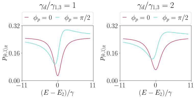
by adding the dephasing rate in the denominator Sheremet et al. (2023). We plot the transmission as in Fig. 3 for two different dephasing rates in Fig. 4. We only include the plot as the dephasing effect on is equivalent. We pick the ratio of the pure dephasing rates over the atomic decay rates respectively. We see that when losses are added, the spectra broadens as expected. The peak size of the transmission dip decreases by and respectively compared to the case with no dephasing rate in Fig. 3. In general, the effect that we report in the paper remains the same if .
References
- Zakka-Bajjani et al. (2011) E. Zakka-Bajjani, F. Nguyen, M. Lee, L. R. Vale, R. W. Simmonds, and J. Aumentado, “Quantum superposition of a single microwave photon in two different ’colour’ states,” Nature Physics 7, 599–603 (2011).
- Clemmen et al. (2016) S. Clemmen, A. Farsi, S. Ramelow, and A. L. Gaeta, “Ramsey interference with single photons,” Phys. Rev. Lett. 117, 223601 (2016).
- Aguayo-Alvarado et al. (2022) A. L. Aguayo-Alvarado, F. Domínguez-Serna, W. De La Cruz, and K. Garay-Palmett, “An integrated photonic circuit for color qubit preparation by third-order nonlinear interactions,” Scientific Reports 12, 5154 (2022).
- Tanzilli et al. (2005) S. Tanzilli, W. Tittel, M. Halder, O. Alibart, P. Baldi, N. Gisin, and H. Zbinden, “A photonic quantum information interface,” Nature (London) 437, 116–120 (2005).
- Karnieli and Arie (2018) A. Karnieli and A. Arie, “Frequency domain stern-gerlach effect for photonic qubits and qutrits,” Optica 5, 1297–1303 (2018).
- Lukens and Lougovski (2017) J. M. Lukens and P. Lougovski, “Frequency-encoded photonic qubits for scalable quantum information processing,” Optica 4, 8 (2017).
- Lu et al. (2020) H.-H. Lu, E. M. Simmerman, P. Lougovski, A. M. Weiner, and J. M. Lukens, “Fully arbitrary control of frequency-bin qubits,” Phys. Rev. Lett. 125, 120503 (2020).
- Lu et al. (2019) H.-H. Lu, J. M. Lukens, B. P. Williams, P. Imany, N. A. Peters, A. M. Weiner, and P. Lougovski, “A controlled-not gate for frequency-bin qubits,” npj Quantum Information 5, 1–8 (2019).
- Lu et al. (2018) H.-H. Lu, J. M. Lukens, N. A. Peters, B. P. Williams, A. M. Weiner, and P. Lougovski, “Quantum interference and correlation control of frequency-bin qubits,” Optica 5, 1455–1460 (2018).
- Olislager et al. (2010) L. Olislager, J. Cussey, A. T. Nguyen, P. Emplit, S. Massar, J.-M. Merolla, and K. P. Huy, “Frequency-bin entangled photons,” Phys. Rev. A 82, 013804 (2010).
- Huang and Kumar (1992) J. Huang and P. Kumar, “Observation of quantum frequency conversion,” Phys. Rev. Lett. 68, 2153–2156 (1992).
- Kobayashi et al. (2016) T. Kobayashi, R. Ikuta, S. Yasui, S. Miki, T. Yamashita, H. Terai, T. Yamamoto, M. Koashi, and N. Imoto, “Frequency-domain Hong-Ou-Mandel interference,” Nature Photonics 10, 441–444 (2016).
- Kobayashi et al. (2017) T. Kobayashi, D. Yamazaki, K. Matsuki, R. Ikuta, S. Miki, T. Yamashita, H. Terai, T. Yamamoto, M. Koashi, and N. Imoto, “Mach-zehnder interferometer using frequency-domain beamsplitter,” Opt. Express 25, 12052–12060 (2017).
- McGuinness et al. (2010) H. J. McGuinness, M. G. Raymer, C. J. McKinstrie, and S. Radic, “Quantum frequency translation of single-photon states in a photonic crystal fiber,” Phys. Rev. Lett. 105, 093604 (2010).
- Dmitriev et al. (2017) A. Y. Dmitriev, R. Shaikhaidarov, V. Antonov, T. Hönigl-Decrinis, and O. Astafiev, “Quantum wave mixing and visualisation of coherent and superposed photonic states in a waveguide,” Nature communications 8, 1–6 (2017).
- Knill et al. (2001) E. Knill, R. Laflamme, and G. J. Milburn, “A scheme for efficient quantum computation with linear optics,” Nature (London) 409, 46–52 (2001).
- Javid et al. (2021) U. A. Javid, J. Ling, J. Staffa, M. Li, Y. He, and Q. Lin, “Ultrabroadband entangled photons on a nanophotonic chip,” Phys. Rev. Lett. 127, 183601 (2021).
- Giovannetti et al. (2011) V. Giovannetti, S. Lloyd, and L. Maccone, “Advances in quantum metrology,” Nature Photonics 5, 222–229 (2011), arXiv:1102.2318 [quant-ph] .
- Rinehart et al. (2012) M. Rinehart, Y. Zhu, and A. Wax, “Quantitative phase spectroscopy,” Biomedical optics express 3, 958–965 (2012).
- Yesharim et al. (2022) O. Yesharim, A. Karnieli, S. Jackel, G. Di Domenico, S. Trajtenberg-Mills, and A. Arie, “Observation of the all-optical stern–gerlach effect in nonlinear optics,” Nature Photonics , 1–6 (2022).
- Sheremet et al. (2023) A. S. Sheremet, M. I. Petrov, I. V. Iorsh, A. V. Poshakinskiy, and A. N. Poddubny, “Waveguide quantum electrodynamics: Collective radiance and photon-photon correlations,” Rev. Mod. Phys. 95, 015002 (2023).
- Roy et al. (2017) D. Roy, C. M. Wilson, and O. Firstenberg, “Colloquium: Strongly interacting photons in one-dimensional continuum,” Rev. Mod. Phys. 89, 021001 (2017).
- Türschmann et al. (2019) P. Türschmann, H. L. Jeannic, S. F. Simonsen, H. R. Haakh, S. Götzinger, V. Sandoghdar, P. Lodahl, and N. Rotenberg, “Coherent nonlinear optics of quantum emitters in nanophotonic waveguides,” Nanophotonics 8, 1641–1657 (2019).
- Chang et al. (2018) D. E. Chang, J. S. Douglas, A. González-Tudela, C.-L. Hung, and H. J. Kimble, “Colloquium: Quantum matter built from nanoscopic lattices of atoms and photons,” Rev. Mod. Phys. 90, 031002 (2018).
- Djotyan et al. (2008) G. P. Djotyan, J. S. Bakos, G. Demeter, Z. Sörlei, J. Szigeti, and D. Dzsotjan, “Creation of a coherent superposition of quantum states by a single frequency-chirped short laser pulse,” J. Opt. Soc. Am. B 25, 166–174 (2008).
- He et al. (2009) J. He, Y.-S. Zhang, X.-F. Zhou, Q.-F. Chen, and G.-C. Guo, “Arbitrary quantum superposition state for three-level system using oscillating dark states,” Optics Communications 282, 1167–1170 (2009).
- Randall et al. (2018) J. Randall, A. M. Lawrence, S. C. Webster, S. Weidt, N. V. Vitanov, and W. K. Hensinger, “Generation of high-fidelity quantum control methods for multilevel systems,” Phys. Rev. A 98, 043414 (2018).
- Martens et al. (2013) C. Martens, P. Longo, and K. Busch, “Photon transport in one-dimensional systems coupled to three-level quantum impurities,” New Journal of Physics 15, 083019 (2013).
- Chan et al. (2022) M. L. Chan, Z. Aqua, A. Tiranov, B. Dayan, P. Lodahl, and A. S. Sørensen, “Quantum state transfer between a frequency-encoded photonic qubit and a quantum-dot spin in a nanophotonic waveguide,” Phys. Rev. A 105, 062445 (2022).
- Bradford and Shen (2012) M. Bradford and J.-T. Shen, “Single-photon frequency conversion by exploiting quantum interference,” Phys. Rev. A 85, 043814 (2012).
- Shen and Fan (2005) J. T. Shen and S. Fan, “Coherent photon transport from spontaneous emission in one-dimensional waveguides,” Optics Letters 30, 2001–2003 (2005).
- Witthaut and Sørensen (2010) D. Witthaut and A. S. Sørensen, “Photon scattering by a three-level emitter in a one-dimensional waveguide,” New Journal of Physics 12, 043052 (2010).
- Shen and Fan (2007) J.-T. Shen and S. Fan, “Strongly correlated multiparticle transport in one dimension through a quantum impurity,” Phys. Rev. A 76, 062709 (2007).
- Schuster et al. (2005) D. I. Schuster, A. Wallraff, A. Blais, L. Frunzio, R.-S. Huang, J. Majer, S. M. Girvin, and R. J. Schoelkopf, “ac stark shift and dephasing of a superconducting qubit strongly coupled to a cavity field,” Phys. Rev. Lett. 94, 123602 (2005).
- Manga Rao and Hughes (2007) V. S. C. Manga Rao and S. Hughes, “Single quantum-dot purcell factor and factor in a photonic crystal waveguide,” Phys. Rev. B 75, 205437 (2007).
- Rephaeli and Fan (2012) E. Rephaeli and S. Fan, “Stimulated emission from a single excited atom in a waveguide,” Phys. Rev. Lett. 108, 143602 (2012).
- Shen and Fan (2009) J.-T. Shen and S. Fan, “Theory of single-photon transport in a single-mode waveguide. ii. coupling to a whispering-gallery resonator containing a two-level atom,” Phys. Rev. A 79, 023838 (2009).
- Hempel et al. (2013) C. Hempel, B. P. Lanyon, P. Jurcevic, R. Gerritsma, R. Blatt, and C. F. Roos, “Entanglement-enhanced detection of single-photon scattering events,” Nature Photonics 7, 630–633 (2013), arXiv:1304.3270 [quant-ph] .
- Reim et al. (2011) K. F. Reim, P. Michelberger, K. C. Lee, J. Nunn, N. K. Langford, and I. A. Walmsley, “Single-photon-level quantum memory at room temperature,” Phys. Rev. Lett. 107, 053603 (2011).
- Chen et al. (2008) Y.-A. Chen, S. Chen, Z.-S. Yuan, B. Zhao, C.-S. Chuu, J. Schmiedmayer, and J.-W. Pan, “Memory-built-in quantum teleportation with photonic and atomic qubits,” Nature Physics 4, 103–107 (2008), arXiv:0705.1256 [quant-ph] .
- Hwang et al. (2009) J. Hwang, M. Pototschnig, R. Lettow, G. Zumofen, A. Renn, S. Götzinger, and V. Sandoghdar, “A single-molecule optical transistor,” Nature (London) 460, 76–80 (2009).
- Vitanov et al. (1999) N. V. Vitanov, K. A. Suominen, and B. W. Shore, “Creation of coherent atomic superpositions by fractional stimulated Raman adiabatic passage,” Journal of Physics B Atomic Molecular Physics 32, 4535–4546 (1999).
- Fan and Joannopoulos (2002) S. Fan and J. D. Joannopoulos, “Analysis of guided resonances in photonic crystal slabs,” Physical Review B 65 (2002), 10.1103/physrevb.65.235112.
- Berman and O’Connell (2005) P. R. Berman and R. C. O’Connell, “Constraints on dephasing widths and shifts in three-level quantum systems,” Phys. Rev. A 71, 022501 (2005).
- Liu et al. (2020) J. Liu, J. Wu, Y. Hu, Y. Zhang, and J. Zhang, “Experimental demonstration of quantum interference modulation via precise dephasing control in atoms,” Optics Communications 466, 125655 (2020).
- Ruostekoski and Javanainen (2017) J. Ruostekoski and J. Javanainen, “Arrays of strongly coupled atoms in a one-dimensional waveguide,” Phys. Rev. A 96, 033857 (2017).