Exact spectral function of the Tonks-Girardeau gas at finite temperature

Abstract

We report on the derivation of determinant representations for the Green’s functions and spectral function of the trapped Tonks-Girardeau gas on the lattice and in the continuum. Our results are valid for any type of statistics of the constituent particles, at zero and finite temperature and arbitrary confining potentials, including nonequilibrium scenarios induced by sudden changes of the external potential. In addition, they are also extremely efficient and easy to implement numerically with the main computational effort being represented by the calculation of partial overlaps of the dynamically evolved single particle wavefunctions. In the lattice case we show that the spectral function of a system with a strong harmonic potential presents only two singular lines compared with three singular lines in the case of a homogeneous system.

I Introduction

Due to the unprecedented degree of control over dimensionality, purity, strength of the interaction and statistics of the constituent particles ultracold gases represent an versatile platform which allows for the investigation of many-body physics which would be very difficult to study in solid state systems [1, 2]. The experimental realization with ultracold atomic gases of many physical systems which are well approximated by integrable or weakly broken integrable systems paved the way for the exploration of fundamental theoretical questions regarding the long time dynamics and lack of thermalization in such systems [3, 4].

A paradigmatic model which is now routinely realized in laboratories is the Lieb-Liniger (LL) model [5] which describes one-dimensional (1D) bosons with repulsive contact interactions. In the limit of infinite repulsion the system is in the so-called Tonks-Girardeau (TG) regime [6, 7, 8, 9, 10] which allows for a comprehensive analytical investigation of the correlation functions due to the knowledge of the wavefunctions via the Bose-Fermi mapping [6]. The lattice counterpart of the Tonks-Girardeau gas is represented by hard-core bosons on the lattice (the Bose-Hubbard model with infinite repulsion) or, equivalently, the isotropic XY spin-chain [11] also known as the XX spin-chain. The generalizations of the Lieb-Liniger and lattice Bose-Hubbard models to arbitrary statistics were introduced in [12, 13, 14, 15, 16] and several proposals of experimental realizations of such interesting systems with ultracold atoms were proposed using Raman assisted tunneling [15, 17], periodically driven lattices [18] or multicolor lattice-depth modulation [19, 20].

In the study of many-body systems the Green’s functions and spectral function (the imaginary part of the retarded Green’s function) are of primary importance [21]. In particular, the spectral function provides fundamental information about the momentum distribution and elementary excitations of the system. While in solid state systems the spectral function is usually accessed using angle-resolved photoemission spectroscopy (ARPES) [22] in the case of ultracold gases it has been measured by radio-frequency spectroscopy [23, 24] and its momentum-resolved extension [25, 26], Bragg spectroscopy [27], lattice modulation spectroscopy [28, 29] and, recently, an ARPES analogue has also been proposed [30].

In the case of systems of impenetrable particles in 1D knowledge of the wavefunctions, which can be obtained using the Bose-Fermi [6, 31] or Anyon-Fermi [32, 33] mappings, opens the way for the derivation of determinant representations for the Green’s functions. These representations, as Toeplitz [6, 34, 35, 36, 37, 38, 39] or Hankel [40, 41, 42, 43, 44, 45] determinants for homogenous or harmonically trapped finite size systems or as Fredholm determinants [46, 47, 48, 49, 50, 51, 52, 53] for systems in the thermodynamic limit, are extremely easy to implement numerically but they also represent the starting point for the derivation of rigorous analytical results. In general the integral operators of the Fredholm determinants describing the correlators of impenetrable particles are of a special type called integrable integral operators and due to their special structure they allow for the derivation of classical integrable differential equations for the correlators and the investigation of the asymptotics by solving an associated Riemann-Hilbert problem [54, 55, 56, 57, 58, 59]. Other methods for deriving the asymptotics from the determinant representations are the use of Szegö’s theorem and Fisher-Hartwig conjecture [60, 35, 36, 37, 41, 38, 39, 61], momentum space approach [62], connections with Painlevé transcendents [63, 41, 42], the replica method [64, 65, 66, 43], form factor expansions at zero [67, 68, 69] and finite temperature [70, 71] or the effective form factor approach [72, 53, 73].

In this article we derive determinant representations for the space-, time-, and temperature-dependent Green’s functions and spectral function for a 1D system of impenetrable particles of arbitrary statistics in the presence of a confining potential. These representations, for both lattice and continuum systems, are also valid in nonequilibrium scenarios due to rapid changes of the confining potential or in the case in which the initial state is not an eigenstate of the final Hamiltonian. Our results, obtained via summation of the form factors, represent the generalization at finite temperature and arbitrary statistics of the representations obtained by Settino et al. [74] for bosonic systems at zero temperature and in nonequilibrium scenarios the equal time correlators reduce to the results derived in [75, 76, 77]. Using an elegant operatorial method [78] Wang derived in [79] similar equivalent representations but only in the case of time-independent external potentials. In addition to being the starting point for the analytical analysis of the asymptotic properties our determinant representations have the advantage of being extremely easy and fast to implement numerically with the main quantities which need to be computed being the partial overlaps of the dynamically evolving single particle basis. This allows us to show numerically that while in the case of a homogeneous system on the latice the spectral function of a system of hard-core bosons presents three singular lines (the first two corresponding to the Type I and Type II excitations in Lieb’s classification [80] and the third one due to the presence of the lattice [74]) the addition of a harmonic potential has a significant effect on the relative weights and positions of each spectral line. As the curvature of the potential increases the spectral weight of one of the lines diminishes approaching zero while a Mott insulator region develops in the center of the trap.

The plan of the paper is as follows. In Sect. II we introduce the anyonic TG gas in the continuum and present the eigenstates and their dynamics. The determinant representation for the correlators at finite temperature obtained via summation of the form factors is presented in Sect. III. The lattice counterpart of the continuum TG gas is introduced in Sect. IV and the results for the lattice correlators can be found in Sect. V. In Sect. VI we compare our results with previous representations derived in the literature in certain limits and in Sect. VII we present and discuss numerical results for the spectral function of a lattice TG gas with harmonic trapping. We conclude in Sect. VIII. Some technical details regarding the equal time limit of one correlation function can be found in Appendix A.

II The anyonic Tonks-Girardeau gas in the continuum

In this paper we will derive determinant representations for the correlators of 1D impenetrable particles with arbitrary statistics in the continuum and on the lattice. We start with the case of continuum systems. A system of $N$ anyons in the continuum with repulsive contact interactions in the presence of an external confining potential $V(x,t)$ is described by the Hamiltonian

$$\mathcal{H}=\int dx\,\frac{\hbar^{2}}{2m}(\partial_{x}\Psi^{\dagger})(\partial_{x}\Psi)+g\,\Psi^{\dagger}\Psi^{\dagger}\Psi\Psi+(V(x,t)-\mu)\,\Psi^{\dagger}\Psi\,,$$ (1)

where the anyonic fields $\Psi^{\dagger}(x),\Psi(x)$ satisfy the commutation relations

$$\Psi(x)\Psi^{\dagger}(y) =-e^{-i\pi\kappa\,\mbox{\small{sign}}(x-y)}\Psi^{\dagger}(y)\Psi(x)+\delta(x-y)\,,$$ (2a)

$$\Psi(x)\Psi(y) =-e^{i\pi\kappa\,\mbox{\small{sign}}(x-y)}\Psi(y)\Psi(x)\,,$$ (2b)

with $\kappa\in[0,1]$ the statistics parameter and $\mbox{{sign}}(x)=|x|/x\,,\mbox{{sign}}(0)=0$. In (1) $\hbar$ is the reduced Planck constant, $m$ is the mass of the particles, $\mu$ the chemical potential and $g$ is the strength of the repulsive interaction. The commutation relations (2) are fermionic at coinciding points, $x=y$, and, as we vary the statistics parameter, they interpolate continuously between the bosonic commutation relations for $\kappa=1$ and the fermionic anticommutation relations for $\kappa=0$. We will consider a particular type of time-dependent confining potentials $V(x,t)$ which describe certain quantum quenches. More precisely we will consider scenarios in which at $t=0$ the system is described by $V(x,t=0)=V_{I}(x)$ and for $t>0$ we have $V(x,t>0)=V_{F}(x)$. For example, the experimentally relevant situation of a system released from an harmonic trap is described by $V(x,t=0)=m\omega_{0}^{2}x^{2}/2$ and $V(x,t>0)=0$. We will denote the initial Hamiltonian by $\mathcal{H}_{I}$ and the final Hamiltonian which governs the subsequent dynamics after the quench by $\mathcal{H}_{F}$. For time-independent Hamiltonians we obviously have $\mathcal{H}_{I}=\mathcal{H}_{F}$.

In the absence of an external potential the Hamiltonian (1) describes the integrable anyonic Lieb-Liniger model [12, 13, 81, 16] which is the natural generalization to arbitrary statistics of the bosonic Lieb-Liniger model [5] (see also [54, 82] and references therein). The realization that integrable and near-integrable systems do not thermalize [83, 84, 85] sparked renewed interest in the nonequilibrium dynamics of such systems. The dynamics of the LL model in various nonequilibrium scenarios has been studied intensely in the last decade see [86, 87, 88, 89, 90, 91, 92, 93, 94, 95, 96, 97, 98, 99, 100, 101, 102, 103, 104, 105, 106, 107, 108, 109, 110, 112, 111, 113, 114, 115, 116]. When $V(x,t)\neq 0$ the Hamiltonian (1) is no longer integrable except when $g=0$ and in the impenetrable limit $g=\infty$ also known as the Tonks-Girardeau regime. This regime of very strong repulsive interaction will be the main focus of this paper. At $t=0$ the eigenstates of the system described by $\mathcal{H}_{I}$ are [54, 81, 77]

$$|\bm{\psi}_{N}(\bm{k})\rangle= \frac{1}{\sqrt{N!}}\int dx_{1}\cdots dx_{N}\,\psi_{N}(x_{1},\cdots,x_{N}|\bm{k})\Psi^{\dagger}(x_{N})\cdots\Psi^{\dagger}(x_{1})|0\rangle\,,$$ (3)

where $|0\rangle$ is the Fock vacuum satisfying $\Psi(x)|0\rangle=\langle 0|\Psi^{\dagger}(x)=0$ for all $x$ and $\langle 0|0\rangle=1$. Each eigenstate is indexed by a set of integers $\bm{k}=(k_{1},\cdots,k_{N})$ and the many-body anyonic wavefunction is determined using the Anyon-Fermi mapping [32, 33] which allows us to write it in terms of the wavefunction of noninteracting fermions subjected to the same external potential

$$\psi_{N}(x_{1},\cdots,x_{N}|\bm{k})=\frac{i^{N(N-1)/2}}{\sqrt{N!}}\prod_{1\leq a<b\leq N}e^{i\frac{\pi\kappa}{2}\,\mbox{\small{sign}}(x_{a}-x_{b})}\det\left[\phi_{k_{a}}(x_{b})\right]_{a,b=1,\cdots,N}\,,$$ (4)

with $\phi_{k}(x)$ the eigenfunctions of the initial single-particle Hamiltonian $\mathcal{H}_{I}^{\mbox{\tiny{SP}}}(x)=-(\hbar^{2}/2m)(\partial^{2}/\partial x^{2})+V(x,t=0)$ i.e., $\mathcal{H}_{I}^{\mbox{\tiny{SP}}}(x)\phi_{k}(x)=\varepsilon(k)\phi_{k}(x)$ and $\varepsilon(k)$ the single particle dispersion relation. Using $e^{i\frac{\pi\kappa}{2}\mbox{\small{sign}}(x_{a}-x_{b})}=\cos(\pi\kappa/2)+i\,\mbox{sign}(x_{a}-x_{b})\sin(\pi\kappa/2)$ it is easy to see that (4) reproduces the bosonic result [6, 47] when $\kappa=1$ and satisfies

$$\psi_{N}(\cdots,x_{i},x_{i+1},\cdots|\bm{k})= -e^{i\pi\kappa\,\mbox{\small{sign}}(x_{i}-x_{i+1})}\psi_{N}(\cdots,x_{i+1},x_{i},\cdots|\bm{k})\,.$$ (5)

being symmetric(anti-symmetric) under the permutation of two particles when the system is bosonic $(\kappa=1)$ [fermionic $(\kappa=0)$]. For an anyonic system, $\kappa\in(0,1)$, Eq. (5) indicates that the space-reversal symmetry is broken resulting in a non-symmetric momentum distribution. The eigenstates (3) form a complete set, are normalized $\langle\bm{\psi}_{N}(\bm{k})|\bm{\psi}_{N}(\bm{k^{\prime}})\rangle=\delta_{\bm{k},\bm{k^{\prime}}}$ and satisfy

$$\mathcal{H}_{I}|\bm{\psi}_{N}(\bm{k})\rangle=E_{N}(\bm{k})|\bm{\psi}_{N}(\bm{k})\rangle\ \ \mbox{ with }E_{N}(\bm{k})=\sum_{i=1}^{N}(\varepsilon(k_{i})-\mu)\,.$$ (6)

In order to compute the form factors and, subsequently, the correlators we will also need $|\bm{\psi}_{N}(\bm{k,t})\rangle=e^{-it\mathcal{H}_{F}}|\bm{\psi}_{N}(\bm{k})\rangle$. In the case of a time-independent external potential ($\mathcal{H}_{I}=\mathcal{H}_{F}$) the time-evolved eigenstate $|\bm{\psi}_{N}(\bm{k,t})\rangle$ is defined by a similar expression with (3) with the time-dependent many-body wavefunction given by [86, 77]

$$\psi_{N}(x_{1},\cdots,x_{N}|\bm{k},t)=\frac{i^{N(N-1)/2}}{\sqrt{N!}}\prod_{1\leq a<b\leq N}e^{i\frac{\pi\kappa}{2}\,\mbox{\small{sign}}(x_{a}-x_{b})}\det\left[\phi_{k_{a}}(x_{b},t)\right]_{a,b=1,\cdots,N}\,,$$ (7)

where $\phi_{k}(x,t)=e^{-i\varepsilon(k)t}\phi_{k}(x)$. In the case of a quantum quench ($\mathcal{H}_{I}\neq\mathcal{H}_{F}$) the many-body wavefunction is also given by (7) with $\phi_{k}(x,t)$ being the unique time-dependent solution of the Schrödinger equation $i\hbar\partial\phi_{j}(x,t)/\partial t=H_{F}^{\mbox{\tiny{SP}}}(x)\phi_{j}(x,t)$ with $H_{F}^{\mbox{\tiny{SP}}}(x)=-(\hbar^{2}/2m)(\partial^{2}/\partial x^{2})+V(x,t>0)$ and initial condition $\phi_{k}(x,0)=\phi_{k}(x)$ [remember that $\phi_{k}(x)$ are eigenfunctions of the initial single-particle Hamiltonian $\mathcal{H}_{I}^{\mbox{\tiny{SP}}}(x)=-(\hbar^{2}/2m)(\partial^{2}/\partial x^{2})+V(x,t=0)$].

Finally, let us give some concrete examples of systems which can be considered:

Harmonic trapping: $V_{I}(x)=m\omega^{2}x^{2}/2$. In this case the single particle functions are the Hermite functions

$$\phi_{k}(x)=e^{-m\omega^{2}x^{2}/2}\frac{1}{\sqrt{2^{k}k!}}\left(\frac{m\omega}{\pi}\right)^{1/4}H_{k}(\sqrt{m\omega}\,x)\,,\ k=0,1,2,\cdots$$ (8)

with $\varepsilon(k)=\hbar\omega(k+1/2)$.

Triangular potential: $V_{I}(x)=|x|$ (Chap. 8.1.2 of [117]). In this case for $k$ even $(2,4,\cdots)$ the single particle functions are

$$\phi_{k}(x)=\left(\frac{2m}{\hbar^{2}}\right)^{1/6}\frac{1}{\sqrt{-a_{k}^{\prime}}Ai(a_{k}^{\prime})}Ai\left[\left(\frac{2m}{\hbar^{2}}\right)^{1/3}(|x|-\varepsilon(k))\right]\,,\ \varepsilon(k)=-a_{k+1}^{\prime}\left(\frac{\hbar^{2}}{2m}\right)^{1/3}\,,$$ (9)

while for $k$ odd $(1,3,\cdots)$ the functions are

$$\phi_{k}(x)=\mbox{sign}(x)\left(\frac{2m}{\hbar^{2}}\right)^{1/6}\frac{1}{Ai^{\prime}(a_{k})}Ai\left[\left(\frac{2m}{\hbar^{2}}\right)^{1/3}(|x|-\varepsilon(k))\right]\,,\ \varepsilon(k)=-a_{k+1}\left(\frac{\hbar^{2}}{2m}\right)^{1/3}\,,$$ (10)

where $Ai(x)=\frac{1}{2\pi}\int_{-\infty}^{+\infty}e^{i(z^{3}/3+xz)}\,dz$ is the Airy function and $a_{k}$ and $a_{k}^{\prime}$ are the k-th zeros of $Ai(x)$ and $Ai^{\prime}(x)$ respectively.

Dirichlet boundary conditions: The single particle functions satisfy $\phi_{k}(0)=\phi_{k}(L)=0$ (the system is defined on $[0,L]$) and are given by

$$\phi_{k}(x)=\sqrt{\frac{2}{L}}\sin\left(\frac{\pi kx}{L}\right)\,,k=1,2,\cdots\,,\ \ \ \ \varepsilon(k)=\frac{\hbar^{2}}{2m}\frac{\pi^{2}k^{2}}{L^{2}}\,.$$ (11)

Neumann boundary conditions: The single particle functions satisfy $\frac{d\phi_{k}}{dx}(0)=\frac{d\phi_{k}}{dx}(L)=0$ (the system is defined on $[0,L]$) and are given by

$$\phi_{k}(x)=\left\{\begin{array}[]{ll}\frac{1}{\sqrt{L}}&k=0\\ \frac{2}{\sqrt{L}}\cos\left(\frac{\pi kx}{L}\right)&k=1,2,\cdots\,,\end{array}\right.\varepsilon(k)=\frac{\hbar^{2}}{2m}\frac{\pi^{2}k^{2}}{L^{2}}\,.$$ (12)

We should point out that our formalism is not valid for systems with no confining potential and periodic boundary conditions. In this case determinant representations for the correlators can be found in [34, 47, 48, 54, 38, 39, 49].

III Determinant representations for finite temperature correlators in the continuum

In this section we will derive determinant representations for the space-, time-, and temperature-dependent field-field correlators of impenetrable particles in the continuum which can be investigated numerically or constitute the starting point for the analytic investigation of their asymptotic behaviour. More precisely, we are interested in

$$g^{(-)}(x,t;y,t^{\prime}) =\langle\Psi^{\dagger}(x,t)\Psi(y,t^{\prime})\rangle_{\mu,T}\,,$$

$$=\mbox{Tr}\left[e^{-\mathcal{H}_{I}/T}\Psi^{\dagger}(x,t)\Psi(y,t^{\prime})\right]/\mbox{Tr}\left[e^{-\mathcal{H}_{I}/T}\right]\,,$$

$$=\sum_{N=0}^{\infty}\,\sum_{k_{1}<\cdots<k_{N+1}}e^{-E_{N+1}(\bm{k})/T}\langle\bm{\psi}_{N+1}(\bm{k})|\Psi^{\dagger}(x,t)\Psi(y,t^{\prime})|\bm{\psi}_{N+1}(\bm{k})\rangle/\sum_{N=0}^{\infty}\,\sum_{k_{1}<\cdots<k_{N}}e^{-E_{N}(\bm{k})/T}\,,$$ (13)

and

$$g^{(+)}(x,t;y,t^{\prime}) =\langle\Psi(x,t)\Psi^{\dagger}(y,t^{\prime})\rangle_{\mu,T}\,,$$

$$=\mbox{Tr}\left[e^{-\mathcal{H}_{I}/T}\Psi(x,t)\Psi^{\dagger}(y,t^{\prime})\right]/\mbox{Tr}\left[e^{-\mathcal{H}_{I}/T}\right]\,,$$

$$=\sum_{N=0}^{\infty}\,\sum_{q_{1}<\cdots<q_{N}}e^{-E_{N}(\bm{k})/T}\langle\bm{\psi}_{N}(\bm{q})|\Psi(x,t)\Psi^{\dagger}(y,t^{\prime})|\bm{\psi}_{N}(\bm{q})\rangle/\sum_{N=0}^{\infty}\,\sum_{q_{1}<\cdots<q_{N}}e^{-E_{N}(\bm{q})/T}\,,$$ (14)

where $\Psi^{\dagger}(x,t)=e^{i\mathcal{H}_{F}t}\Psi^{\dagger}(x)e^{-i\mathcal{H}_{F}t}$ and $\Psi(x,t)=e^{i\mathcal{H}_{F}t}\Psi(x)e^{-i\mathcal{H}_{F}t}$. These are the field-field correlators evaluated in a thermal state of the initial Hamiltonian $\mathcal{H}_{I}$ described by the grandcanonical ensemble at temperature $T$ and chemical potential $\mu$. In equilibrium we have $\mathcal{H}_{I}=\mathcal{H}_{F}$ while in a quench scenario the subsequent time evolution of the fields is described by the final Hamiltonian $\mathcal{H}_{F}$. The field correlators (III) and (III) allow us to describe the usual six Green’s functions (advanced, retarded, time-ordered, anti-time-ordered, greater, lesser) usually employed in the study of many-body systems (see Chap. 2.9.1 of [21]). In particular, the greater and lesser Green’s functions are given by

$$G^{>}(x,t;y,t^{\prime}) =-i\langle\Psi(x,t)\Psi^{\dagger}(y,t^{\prime})\rangle_{\mu,T}=-ig^{(+)}(x,t;y,t^{\prime})\,,$$ (15)

$$G^{<}(x,t;y,t^{\prime}) =-i\langle\Psi^{\dagger}(y,t^{\prime})\Psi(x,t)\rangle_{\mu,T}=-ig^{(-)}(y,t^{\prime};x,t)\,,$$ (16)

and the retarded Green’s function is

$$G^{R}(x,t;y,t^{\prime})= \,\Theta(t-t^{\prime})\left[G^{>}(x,t;y,t^{\prime})+G^{<}(x,t;y,t^{\prime})\right]\,,$$ (17)

$$= -i\,\Theta(t-t^{\prime})\left[g^{(+)}(x,t;y,t^{\prime})+g^{(-)}(y,t^{\prime};x,t)\right]\,,$$ (18)

where $\Theta(t)$ is the Heaviside function. The spectral function is the imaginary part of the Fourier transform of the retarded Green’s function

$$A(k,\omega)=-\frac{1}{\pi}\mbox{Im}\,G^{R}(k,\omega)\,,$$ (19)

with

$$G^{R}(k,\omega)=\int_{-\infty}^{+\infty}\,dt\,e^{i\omega t}\int_{-\infty}^{+\infty}\int_{-\infty}^{+\infty}\,dxdy\,e^{-ik(x-y)}G^{R}(x,t;y,0)\,.$$ (20)

The density and the momentum distribution of the system are given by $\rho(x,t)=g^{(-)}(x,t;x,t)$ and $n(k,t)=\int_{-\infty}^{+\infty}\int_{-\infty}^{+\infty}\,dxdy\,e^{-ik(x-y)}g^{(-)}(x,t;y,t)$, respectively.

III.1 Form factors

In order to derive determinant representations for the field correlators (III) and (III) we are going to employ the summation of form factors [48, 54]. We are going to compute first the form factors for a finite size system and express the mean value of bilocal operators in an arbitrary state as a sum over them. The summation can be performed using a well known technique known as the “insertion of summation under the determinant”[48, 54] (this can be understood as an application of a slightly modified Cauchy-Binet formula [74]) which will allow the derivation of a single determinant for the mean value. The final result valid in the thermodynamic limit is obtained using von Koch’s formula.

We start with the computation of the form factors for a finite size system. Inserting a resolution of the identity in each mean value of bilocal operators appearing in (III) and (III) we obtain (the bar denotes complex conjugation)

$$\langle\bm{\psi}_{N+1}(\bm{k})|\Psi^{\dagger}(x,t)\Psi(y,t^{\prime})|\bm{\psi}_{N+1}(\bm{k})\rangle =\sum_{q_{1}<\cdots<q_{N}}\underbrace{\langle\bm{\psi}_{N+1}(\bm{k})|\Psi^{\dagger}(x,t)|\bm{\psi}_{N}(\bm{q})\rangle}_{\overline{F}_{N}(\bm{k},\bm{q}|x,t)}\underbrace{\langle\bm{\psi}_{N}(\bm{q})|\Psi(y,t^{\prime})|\bm{\psi}_{N+1}(\bm{k})\rangle}_{F_{N}(\bm{k},\bm{q}|y,t^{\prime})}\,,$$ (21)

$$\langle\bm{\psi}_{N}(\bm{q})|\Psi(x,t)\Psi^{\dagger}(y,t^{\prime})|\bm{\psi}_{N}(\bm{q})\rangle =\sum_{k_{1}<\cdots<k_{N+1}}\underbrace{\langle\bm{\psi}_{N}(\bm{q})|\Psi(x,t)|\bm{\psi}_{N+1}(\bm{k})\rangle}_{F_{N}(\bm{k},\bm{q}|x,t)}\underbrace{\langle\bm{\psi}_{N+1}(\bm{k})|\Psi^{\dagger}(y,t^{\prime})|\bm{\psi}_{N}(\bm{q})\rangle}_{\overline{F}_{N}(\bm{k},\bm{q}|y,t^{\prime})}\,,$$ (22)

which shows that each of this quantities can be expressed as sums over form factors which are defined as

$$F_{N}(\bm{k},\bm{q}|x,t)=\langle\bm{\psi}_{N}(\bm{q})|\Psi(x,t)|\bm{\psi}_{N+1}(\bm{k})\rangle\,,$$ (23)

where $\bm{k}=(k_{1},\cdots,k_{N+1})$ and $\bm{q}=(q_{1},\cdots,q_{N})$ describe arbitrary states with $N+1$ and $N$ particles, respectively. Note that we need to define only the form factor of the $\Psi(x,t)$ operator, the equivalent quantity for the creation operator $\Psi^{\dagger}(x,t)$ is given by the complex conjugate of $F_{N}(\bm{k},\bm{q}|x,t)$. Using the equal-time commutation relations (2) and the definition of the eigenstates (3) we obtain

$$F_{N}(\bm{k},\bm{q}|x,t)=e^{i\mu t}\sqrt{N+1}\int_{L_{-}}^{L_{+}}dx_{1}\cdots dx_{N}\psi_{N+1}(x_{1},\cdots,x_{N},x|\bm{k},t)\overline{\psi}_{N}(x_{1},\cdots,x_{N}|\bm{q},t)\,,$$ (24)

with

$$\psi_{N+1}(x_{1},\cdots,x_{N},x|\bm{k},t) =\frac{i^{N(N+1)/2}}{\sqrt{(N+1)!}}\left(\prod_{1\leq a<b\leq N}e^{i\frac{\pi\kappa}{2}\mbox{\small{sign}}(x_{a}-x_{b})}\right)\left(\prod_{j=1}^{N}e^{i\frac{\pi\kappa}{2}\mbox{\small{sign}}(x_{j}-x)}\right)$$

$$\qquad\qquad\qquad\qquad\times\sum_{P\in S_{N+1}}(-1)^{P}\prod_{j=1}^{N}\phi_{k_{P}(j)}(x_{j},t)\phi_{k_{P(N+1)}}(x,t)\,,$$ (25)

$$\overline{\psi}_{N}(x_{1},\cdots,x_{N},|\bm{q},t) =\frac{(-i)^{N(N-1)/2}}{\sqrt{N!}}\left(\prod_{1\leq a<b\leq N}e^{-i\frac{\pi\kappa}{2}\mbox{\small{sign}}(x_{a}-x_{b})}\right)\sum_{Q\in S_{N}}(-1)^{Q}\prod_{j=1}^{N}\overline{\phi}_{q_{Q}(j)}(x_{j},t)\,,$$ (26)

where $S_{N+1}$ is the group of permutations of $N+1$ elements, $(-1)^{P}$ the signature of the permutation and $\phi_{k}(x,t)$ are the time-evolved single particle eigenfunctions (when we do not have a quench we have $\phi_{k}(x,t)=e^{-i\varepsilon(k)t}\phi_{k}(x)$). In (24) $L_{\pm}$ quantify the size of the system which depends on the potential or boundary conditions. For example in the case of a harmonic potential we have $L_{\pm}=\pm\infty$ while in the case of a system with Dirichlet boundary conditions at $0$ and $L$ we have $L_{-}=0$ and $L_{+}=L$. In all cases due to the completeness and orthonormality of the single particle eigenfunctions we have

$$\int_{L_{-}}^{L_{+}}\phi_{k}(v,t)\overline{\phi}_{q}(v,t)\,dv=\delta_{k,q}\,.$$ (27)

Using the explicit form of the wavefunctions (25) and (26) the analytic expression for the form factor (24) can be written as a sum of factorized terms

$$F_{N}(\bm{k},\bm{q}|x,t)=\frac{e^{i\mu t}i^{N}}{N!}\int_{L_{-}}^{L_{+}}dx_{1}\cdots dx_{N}\sum_{P\in S_{N+1}}\sum_{Q\in S_{N}}(-1)^{P+Q}\left(\prod_{j=1}^{N}e^{i\frac{\pi\kappa}{2}\mbox{\small{sign}}(x_{j}-x)}\phi_{k_{P(j)}}(x_{j},t)\overline{\phi}_{q_{Q(j)}}(x_{j},t)\right)\phi_{k_{P(N+1)}}(x,t)\,,$$ (28)

with

$$\int_{L_{-}}^{L_{+}}e^{i\frac{\pi\kappa}{2}\mbox{\small{sign}}(v-x)}\phi_{k}(v,t)\overline{\phi}_{q}(v,t)\,dv =e^{-i\frac{\pi\kappa}{2}}\int_{L_{-}}^{x}\phi_{k}(v,t)\overline{\phi}_{q}(v,t)\,dv+e^{i\frac{\pi\kappa}{2}}\int_{x}^{L_{+}}\phi_{k}(v,t)\overline{\phi}_{q}(v,t)\,dv\,,$$

$$=e^{-i\frac{\pi\kappa}{2}}\left(\delta_{k,q}-(1-e^{i\pi\kappa})\int_{x}^{L_{+}}\phi_{k}(v,t)\overline{\phi}_{q}(v,t)\,dv\right)\,,$$ (29)

where we have used the completeness relation (27). Introducing

$$f(k,q|\kappa,x,t)=\delta_{k,q}-(1-e^{i\pi\kappa})\int_{x}^{L_{+}}\phi_{k}(v,t)\overline{\phi}_{q}(v,t)\,dv\,,$$ (30)

we find

$$F_{N}(\bm{k},\bm{q}|x,t) =\frac{e^{i\mu t}\left(ie^{-i\frac{\pi\kappa}{2}}\right)^{N}}{N!}\sum_{P\in S_{N+1}}\sum_{Q\in S_{N}}(-1)^{P+Q}\left(\prod_{j=1}^{N}f(k_{P(j)},q_{Q(j)}|\kappa,x,t)\right)\phi_{k_{P(N+1)}}(x,t)\,,$$

$$=\frac{e^{i\mu t}\left(ie^{-i\frac{\pi\kappa}{2}}\right)^{N}}{N!}\sum_{Q\in S_{N}}(-1)^{Q}\left|\begin{array}[]{cccc}f(k_{1},q_{Q(1)}|\kappa)&\cdots&f(k_{1},q_{Q(N)}|\kappa)&\phi_{k_{1}}\\ \vdots&\ddots&\vdots&\vdots\\ f(k_{N+1},q_{Q(1)}|\kappa)&\cdots&f(k_{N+1},q_{Q(N)}|\kappa)&\phi_{k_{N+1}}\end{array}\right|(x,t)\,.$$ (34)

For each permutation $Q$ rearranging the columns of the matrix appearing in the last expression $Q\rightarrow(1,\cdots,N)$ gives a $(-1)^{Q}$ factor and for each of the $N!$ permutation we obtain the same result. Therefore, the final result for the form factor is

$$F_{N}(\bm{k},\bm{q}|x,t)=e^{i\mu t}\left(ie^{-i\frac{\pi\kappa}{2}}\right)^{N}\,\det_{N+1}B(\bm{k},\bm{q}|x,t)\,,$$ (35)

where $B$ is a square matrix of dimension $N+1$ with elements

$$B_{ab}(\bm{k},\bm{q}|x,t)=\left\{\begin{array}[]{ll}f(k_{a},q_{b}|\kappa,x,t)\,,&a=1,\cdots,N+1\,,\ \ b=1,\cdots,N\,,\\ \phi_{k_{a}}(x,t)\,,&a=1,\cdots,N+1\,,\ \ b=N+1\,.\\ \end{array}\right.$$ (36)

III.2 Determinant representation for $\langle\bm{\psi}_{N+1}(\bm{k})|\Psi^{\dagger}(x,t)\Psi(y,t^{\prime})|\bm{\psi}_{N+1}(\bm{k})\rangle$

We can obtain a determinant representation for the mean values of bilocal operators appearing in the definition of the correlation functions (III) and (III) by using the explicit formula for the form factors (35) and the “insertion of summation under the determinant” [48, 54]. From (21) we have

$$A^{(-)} \equiv\langle\bm{\psi}_{N+1}(\bm{k})|\Psi^{\dagger}(x,t)\Psi(y,t^{\prime})|\bm{\psi}_{N+1}(\bm{k})\rangle=\sum_{q_{1}<\cdots<q_{N}}\overline{F}_{N}(\bm{k},\bm{q}|x,t)F_{N}(\bm{k},\bm{q}|y,t^{\prime})\,,$$

$$=e^{-i\mu(t-t^{\prime})}\sum_{q_{1}<\cdots<q_{N}}\overline{\det_{N+1}B(\bm{k},\bm{q}|x,t)}\det_{N+1}B(\bm{k},\bm{q}|y,t^{\prime})\,.$$ (37)

The product of the two determinants is symmetric in $q$’s and vanishes when two of them are equal, therefore we can write

$$A^{(-)} =\frac{e^{-i\mu(t-t^{\prime})}}{N!}\sum_{q_{1}=1}^{\infty}\cdots\sum_{q_{N}=1}^{\infty}\overline{\det_{N+1}B(\bm{k},\bm{q}|x,t)}\det_{N+1}B(\bm{k},\bm{q}|y,t^{\prime})\,,$$

$$=\frac{e^{-i\mu(t-t^{\prime})}}{N!}\sum_{q_{1}=1}^{\infty}\cdots\sum_{q_{N}=1}^{\infty}\sum_{P\in S_{N+1}}\sum_{Q\in S_{N+1}}(-1)^{P+Q}\left(\prod_{j=1}^{N}\overline{f}(k_{P(j)},q_{j}|\kappa,x,t)f(k_{Q(j)},q_{j}|\kappa,y,t^{\prime})\right)$$

$$\qquad\qquad\qquad\qquad\qquad\qquad\qquad\qquad\qquad\qquad\qquad\qquad\qquad\qquad\qquad\qquad\times\overline{\phi}_{k_{P(N+1)}}(x,t)\phi_{k_{Q(N+1)}}(y,t^{\prime})\,,$$

$$=\frac{e^{-i\mu(t-t^{\prime})}}{N!}\sum_{q_{1}=1}^{\infty}\cdots\sum_{q_{N}=1}^{\infty}\sum_{R\in S_{N+1}}\sum_{Q\in S_{N+1}}(-1)^{R}\left(\prod_{j=1}^{N}\overline{f}(k_{RQ(j)},q_{j}|\kappa,x,t)f(k_{Q(j)},q_{j}|\kappa,y,t^{\prime})\right)$$

$$\qquad\qquad\qquad\qquad\qquad\qquad\qquad\qquad\qquad\qquad\qquad\qquad\qquad\qquad\qquad\qquad\times\overline{\phi}_{k_{RQ(N+1)}}(x,t)\phi_{k_{Q(N+1)}}(y,t^{\prime})\,.$$ (38)

In the third line of (III.2) we have used the fact that for any two permutations $P$ and $Q$ we have $P=RQ$ with $R$ another permutation. It is easy to see that the last line of (III.2) can be written as

$$A^{(-)} =\frac{e^{-i\mu(t-t^{\prime})}}{N!}\sum_{q_{1}=1}^{\infty}\cdots\sum_{q_{N}=1}^{\infty}\sum_{Q\in S_{N+1}}$$

$$\times\left|\begin{array}[]{cccc}\overline{f}(k_{Q(1)},q_{1}|x,t)f(k_{Q(1)},q_{1}|y,t^{\prime})&\cdots&\overline{f}(k_{Q(1)},q_{N}|x,t)f(k_{Q(1)},q_{N}|y,t^{\prime})&\overline{\phi}_{k_{Q(1)}}(x,t)\phi_{k_{Q(N+1)}}(y,t^{\prime})\\ \vdots&\ddots&\vdots&\vdots\\ \overline{f}(k_{Q(N+1)},q_{1}|x,t)f(k_{Q(1)},q_{1}|y,t^{\prime})&\cdots&\overline{f}(k_{Q(N+1)},q_{N}|x,t)f(k_{Q(1)},q_{N}|y,t^{\prime})&\overline{\phi}_{k_{Q(N+1)}}(x,t)\phi_{k_{Q(N+1)}}(y,t^{\prime})\\ \end{array}\right|\,.$$

Because $q_{i}$ appears only in the $i$-th column we can sum inside the determinant. Introducing two matrices (depending on the state $\bm{k}$)

$$\widetilde{U}_{a,b}^{(-)}(x,t;y,t^{\prime}) =\sum_{q=1}^{\infty}\overline{f}(k_{a},q|\kappa,x,t)f(k_{b},q|\kappa,y,t^{\prime})\,,\qquad a,b=1,\cdots,N+1\,,$$ (39)

$$\widetilde{R}_{a,b}^{(-)}(x,t;y,t^{\prime}) =\overline{\phi}_{k_{a}}(x,t)\phi_{k_{b}}(y,t^{\prime})\,,\qquad a,b=1,\cdots,N+1\,,$$ (40)

the last relation can be written as

$$A^{(-)} =\frac{e^{-i\mu(t-t^{\prime})}}{N!}\sum_{Q\in S_{N+1}}\left|\begin{array}[]{cccc}\widetilde{U}_{Q(1),Q(1)}^{(-)}&\cdots&\widetilde{U}_{Q(1),Q(N)}^{(-)}&\widetilde{R}_{Q(1),Q(N+1)}^{(-)}\\ \vdots&\ddots&\vdots&\vdots\\ \widetilde{U}_{Q(N+1),Q(1)}^{(-)}&\cdots&\widetilde{U}_{Q(N+1),Q(N)}^{(-)}&\widetilde{R}_{Q(N+1),Q(N+1)}^{(-)}\\ \end{array}\right|(x,t;y,t^{\prime})\,,$$ (44)

$$=e^{-i\mu(t-t^{\prime})}\sum_{j=1}^{N+1}\left|\begin{array}[]{ccccc}\widetilde{U}_{1,1}^{(-)}&\cdots&\widetilde{R}_{1,j}^{(-)}&\cdots&\widetilde{U}_{1,N+1}^{(-)}\\ \vdots&\ddots&\vdots&\ddots&\vdots\\ \widetilde{U}_{N+1,1}^{(-)}&\cdots&\widetilde{R}_{N+1,j}^{(-)}&\cdots&\widetilde{U}_{N+1,N+1}^{(-)}\\ \end{array}\right|(x,t;y,t^{\prime})$$ (48)

where in the last line we have reorganized the columns and rows such that $Q\rightarrow(1,\cdots,N+1)$. Using the fact that $\widetilde{R}_{a,b}^{(-)}$ is a rank 1 matrix we can write the final result

$$\langle\bm{\psi}_{N+1}(\bm{k})|\Psi^{\dagger}(x,t)\Psi(y,t^{\prime})|\bm{\psi}_{N+1}(\bm{k})\rangle =e^{-i\mu(t-t^{\prime})}\frac{\partial}{\partial z}\det_{N+1}\left.\left(\widetilde{U}^{(-)}+z\widetilde{R}^{(-)}\right)\right|_{z=0}\,,$$ (49)

$$=e^{-i\mu(t-t^{\prime})}\left[\det_{N+1}\left(\widetilde{U}^{(-)}+\widetilde{R}^{(-)}\right)-\det_{N+1}\widetilde{U}^{(-)}\right]\,.$$ (50)

III.3 Determinant representation for $\langle\bm{\psi}_{N}(\bm{q})|\Psi(x,t)\Psi^{\dagger}(y,t^{\prime})|\bm{\psi}_{N}(\bm{q})\rangle$

Similar to the previous case we can obtain a determinant formula for the mean value of bilocal operators appearing in (III). From (22) we have

$$A^{(+)} \equiv\langle\bm{\psi}_{N}(\bm{q})|\Psi(x,t)\Psi^{\dagger}(y,t^{\prime})|\bm{\psi}_{N}(\bm{q})\rangle=\sum_{k_{1}<\cdots<k_{N+1}}F_{N}(\bm{k},\bm{q}|x,t)\overline{F}_{N}(\bm{k},\bm{q}|y,t^{\prime})\,,$$

$$=e^{i\mu(t-t^{\prime})}\sum_{k_{1}<\cdots<k_{N+1}}\det_{N+1}B(\bm{k},\bm{q}|x,t)\overline{\det_{N+1}B(\bm{k},\bm{q}|y,t^{\prime})}\,.$$ (51)

The product of determinants is symmetric in $k$’s and vanishes when two of them are equal. Therefore the summation over all the states with $N+1$ particles can be written as

$$A^{(+)} =\frac{e^{i\mu(t-t^{\prime})}}{(N+1)!}\sum_{k_{1}=1}^{\infty}\cdots\sum_{k_{N+1}=1}^{\infty}\sum_{P\in S_{N+1}}\sum_{Q\in S_{N+1}}(-1)^{P+Q}\left(\prod_{j=1}^{N}f(k_{P(j)},q_{j}|\kappa,x,t)\overline{f}(k_{Q(j)},q_{j}|\kappa,y,t^{\prime})\right)$$

$$\qquad\qquad\qquad\qquad\qquad\qquad\qquad\qquad\qquad\qquad\qquad\qquad\qquad\qquad\qquad\qquad\times\phi_{k_{P(N+1)}}(x,t)\overline{\phi}_{k_{Q(N+1)}}(y,t^{\prime})\,,$$

$$=\frac{e^{i\mu(t-t^{\prime})}}{(N+1)!}\sum_{k_{1}=1}^{\infty}\cdots\sum_{k_{N+1}=1}^{\infty}\sum_{R\in S_{N+1}}\sum_{Q\in S_{N+1}}(-1)^{R}\left(\prod_{j=1}^{N}f(k_{RQ(j)},q_{j}|\kappa,x,t)\overline{f}(k_{Q(j)},q_{j}|\kappa,y,t^{\prime})\right)$$

$$\qquad\qquad\qquad\qquad\qquad\qquad\qquad\qquad\qquad\qquad\qquad\qquad\qquad\qquad\qquad\qquad\times\phi_{k_{RQ(N+1)}}(x,t)\overline{\phi}_{k_{Q(N+1)}}(y,t^{\prime})\,,$$

$$=\frac{e^{i\mu(t-t^{\prime})}}{(N+1)!}\sum_{k_{1}=1}^{\infty}\cdots\sum_{k_{N+1}=1}^{\infty}\sum_{Q\in S_{N+1}}\left(\prod_{j=1}^{N}\overline{f}(k_{Q(j)},q_{j}|\kappa,y,t^{\prime})\overline{\phi}_{k_{Q(N+1)}}(y,t^{\prime})\right)$$

$$\qquad\qquad\qquad\qquad\qquad\qquad\qquad\times\left|\begin{array}[]{cccc}f(k_{Q(1)},q_{1}|\kappa,x,t)&\cdots&f(k_{Q(1)},q_{N}|\kappa,x,t)&\phi_{k_{Q(1)}}(x,t)\\ \vdots&\ddots&\vdots&\vdots\\ f(k_{Q(N+1)},q_{1}|\kappa,x,t)&\cdots&f(k_{Q(N+1)},q_{N}|\kappa,x,t)&\phi_{k_{Q(N+1)}}(x,t)\end{array}\right|\,.$$ (55)

Like in the previous case in the second line we have expressed the permutations $P$ as a product of $R$ and $Q$. Now we multiply the $j$-th row of the determinant from the third line of (III.3) with $\overline{f}(k_{Q(j)},q_{j}|\kappa,y,t^{\prime})$ and the $N+1$-th row with $\overline{\phi}_{k_{Q(N+1)}}(y,t^{\prime})$ obtaining

$$A^{(+)} =\frac{e^{i\mu(t-t^{\prime})}}{(N+1)!}\sum_{k_{1}=1}^{\infty}\cdots\sum_{k_{N+1}=1}^{\infty}\sum_{Q\in S_{N+1}}$$

$$\times\left|\begin{array}[]{cccc}f(k_{Q(1)},q_{1}|x,t)\overline{f}(k_{Q(1)},q_{1}|y,t^{\prime})&\cdots&f(k_{Q(1)},q_{N}|x,t)\overline{f}(k_{Q(1)},q_{1}|y,t^{\prime})&\phi_{k_{Q(1)}}(x,t)\overline{f}(k_{Q(1)},q_{1}|y,t^{\prime})\\ \vdots&\ddots&\vdots&\vdots\\ f(k_{Q(N)},q_{1}|x,t)\overline{f}(k_{Q(N)},q_{N}|y,t^{\prime})&\cdots&f(k_{Q(N)},q_{N}|x,t)\overline{f}(k_{Q(N)},q_{N}|y,t^{\prime})&\phi_{k_{Q(N)}}(x,t)\overline{f}(k_{Q(N)},q_{N}|y,t^{\prime})\\ f(k_{Q(N+1)},q_{1}|x,t)\overline{\phi}_{k_{Q(N+1)}}(y,t^{\prime})&\cdots&f(k_{Q(N+1)},q_{N}|x,t)\overline{\phi}_{k_{Q(N+1)}}(y,t^{\prime})&\phi_{k_{Q(N+1)}}(x,t)\overline{\phi}_{k_{Q(N+1)}}(y,t^{\prime})\\ \end{array}\right|\,.$$

In the previous expression $k_{Q(j)}$ appears only in the $j$-th row and, therefore, we can sum inside the determinant. Introducing the $\bm{q}=(q_{1},\cdots,q_{n})$ dependent matrix and functions

$$\widetilde{U}_{a,b}^{(+)}(x,t;y,t^{\prime}) =\sum_{k=1}^{\infty}f(k,q_{b}|\kappa,x,t)\overline{f}(k,q_{a}|\kappa,y,t^{\prime})\,,\qquad a,b=1,\cdots,N\,,$$ (56)

$$\widetilde{e}_{a}(x,t;y,t^{\prime}) =\sum_{k=1}^{\infty}f(k,q_{a}|\kappa,x,t)\overline{\phi}_{k}(y,t^{\prime})\,,\qquad a=1,\cdots,N\,,$$ (57)

$$\widetilde{\overline{e}}_{a}(x,t;y,t^{\prime}) =\sum_{k=1}^{\infty}\overline{f}(k,q_{a}|\kappa,y,t^{\prime})\phi_{k}(x,t)\,,\qquad a=1,\cdots,N\,,$$ (58)

together with

$$g(x,t;y,t^{\prime})=\sum_{k=1}^{\infty}\phi_{k}(x,t)\overline{\phi}_{k}(y,t^{\prime})\,,$$ (59)

the last expression can be written as (the sum over the $Q$ permutations produces $(N+1)!$ identical terms)

$$A^{(+)} =e^{i\mu(t-t^{\prime})}\left|\begin{array}[]{cccc}\widetilde{U}_{1,1}^{(+)}&\cdots&\widetilde{U}_{1,N}^{(+)}&\widetilde{\overline{e}}_{1}\\ \vdots&\ddots&\vdots&\vdots\\ \widetilde{U}_{N,1}^{(+)}&\cdots&\widetilde{U}_{N,N}^{(+)}&\widetilde{\overline{e}}_{N}\\ \widetilde{e}_{1}&\cdots&\widetilde{e}_{N}&g\end{array}\right|(x,t;y,t^{\prime})\,.$$

Expanding this result on the last column we obtain our final result

$$\langle\bm{\psi}_{N}(\bm{q})|\Psi(x,t)\Psi^{\dagger}(y,t^{\prime})|\bm{\psi}_{N}(\bm{q})\rangle =e^{i\mu(t-t^{\prime})}\left[g+\frac{\partial}{\partial z}\right]\det_{N}\left.\left(\widetilde{U}^{(+)}-z\widetilde{R}^{(+)}\right)\right|_{z=0}\,,$$ (60)

$$=e^{i\mu(t-t^{\prime})}\left[\det_{N}\left(\widetilde{U}^{(+)}-\widetilde{R}^{(+)}\right)+(g-1)\det_{N}\widetilde{U}^{(+)}\right]\,,$$ (61)

with $\widetilde{R}^{(+)}$ a $\bm{q}$-dependent matrix with elements

$$\widetilde{R}^{(+)}_{a,b}(x,t;y,t^{\prime})=\widetilde{\overline{e}}_{a}(x,t;y,t^{\prime})\widetilde{e}_{b}(x,t;y,t^{\prime})\,,\qquad a,b=1,\cdots,N\,.$$ (62)

III.4 Thermodynamic limit

In order to compute the thermodynamic limit we are going to use von Koch’s determinant formula which states that for any square matrix of dimension $M$ (which can also be infinite) denoted by $A$ and $z$ a bounded complex parameter we have [118]:

$$\det(1+zA) =1+z\sum_{m=1}^{M}A_{m,m}+\frac{z^{2}}{2!}\sum_{m=1}^{M}\sum_{n=1}^{M}\left|\begin{array}[]{cc}A_{m,m}&A_{m,n}\\ A_{n,m}&A_{n,n}\end{array}\right|+\cdots\,.$$ (65)

We start with $g^{(-)}(x,t;y,t^{\prime})$ defined in (III). As a first step we need to compute the partition function $\mathcal{Z}=\mbox{Tr}\left[e^{-\mathcal{H}_{I}/T}\right]$. It is easy to se that [$E_{N}(\bm{k})=\sum_{i=1}^{N}(\varepsilon(k_{i})-\mu)$]

$$\mathcal{Z} =\sum_{N=0}^{\infty}\,\sum_{k_{1}<\cdots<k_{N}}e^{-E_{N}(\bm{k})/T}=\prod_{k=1}^{\infty}\left(1+e^{-(\varepsilon(k)-\mu)/T}\right)\,.$$ (66)

Using the determinant representation for the mean value of the bilocal operator (49) the numerator of (III) can be written as

$$N^{(-)} =\sum_{N=0}^{\infty}\,\sum_{k_{1}<\cdots<k_{N+1}}e^{-E_{N+1}(\bm{k})/T}\langle\bm{\psi}_{N+1}(\bm{k})|\Psi^{\dagger}(x,t)\Psi(y,t^{\prime})|\bm{\psi}_{N+1}(\bm{k})\rangle\,,$$

$$=e^{-i\mu(t-t^{\prime})}\sum_{N=0}^{\infty}\sum_{k_{1}<\cdots<k_{N+1}}e^{-E_{N+1}(\bm{k})/T}\left[\det_{N+1}\left(\widetilde{U}^{(-)}+\widetilde{R}^{(-)}\right)-\det_{N+1}\widetilde{U}^{(-)}\right]\,.$$ (67)

The energy term $e^{-E_{N+1}(\bm{k})/T}=e^{-\sum_{i=1}^{N+1}(\varepsilon(k_{i})-\mu)/T}$ is distributed inside the determinants as follows: the $i$-th row is multiplied by $e^{-(\varepsilon(k_{i})-\mu)/2T}$ while the $j$-th column is multiplied by $e^{-(\varepsilon(k_{j})-\mu)/2T}$. Using von Koch’s determinant formula (65) we obtain for the numerator

$$N^{(-)}=e^{-i\mu(t-t^{\prime})}\left[\det\left(1+\textsf{U}^{(-)}_{M}+\textsf{R}^{(-)}_{M}\right)-\det\left(1+\textsf{U}^{(-)}_{M}\right)\right]\,,$$ (68)

with infinite dimensional determinants and matrices $\textsf{U}^{(-)}_{M}$ and $\textsf{R}^{(-)}_{M}$ defined by

$$[\textsf{U}^{(-)}_{M}]_{a,b}(x,t;y,t^{\prime}) =e^{-(\varepsilon(a)-\mu)/2T}\,\textsf{U}^{(-)}_{a,b}(x,t;y,t^{\prime})\,e^{-(\varepsilon(b)-\mu)/2T}\,,\ \ a,b=1,2,\cdots\ ,$$ (69)

$$[\textsf{R}^{(-)}_{M}]_{a,b}(x,t;y,t^{\prime}) =e^{-(\varepsilon(a)-\mu)/2T}\,\textsf{R}^{(-)}_{a,b}(x,t;y,t^{\prime})\,e^{-(\varepsilon(b)-\mu)/2T}\,,\ \ a,b=1,2,\cdots\ ,$$ (70)

and

$$\textsf{U}_{a,b}^{(-)}(x,t;y,t^{\prime}) =\sum_{q=1}^{\infty}\overline{f}(a,q|\kappa,x,t)f(b,q|\kappa,y,t^{\prime})\,,\ \ a,b=1,2,\cdots\,,$$ (71)

$$\textsf{R}_{a,b}^{(-)}(x,t;y,t^{\prime}) =\overline{\phi}_{a}(x,t)\phi_{b}(y,t^{\prime})\,,\ \ a,b=1,2,\cdots\,.$$ (72)

It is important to note that while $\widetilde{U}_{a,b}^{(-)}(x,t;y,t^{\prime})$, $\widetilde{R}_{a,b}^{(-)}(x,t;y,t^{\prime})$ were finite size matrices that were dependent on particular eigenstates $\bm{k}=(k_{1},\cdots,k_{N+1})$ the matrices $\textsf{U}_{a,b}^{(-)}(x,t;y,t^{\prime})$ and $\textsf{R}_{a,b}^{(-)}(x,t;y,t^{\prime})$ are infinite dimensional. From the numerator (68) we can extract $(1+e^{-(\varepsilon(i)-\mu)/T})^{1/2}$ from the $i$-th row and $(1+e^{-(\varepsilon(j)-\mu)/T})^{1/2}$ from the $j$-th column obtaining an infinite product equal to the partition function (66). In this way we obtain the final result for the $g^{(-)}$ correlator in the thermodynamic limit

$$g^{(-)}(x,t;y,t^{\prime})=e^{-i\mu(t-t^{\prime})}\left[\det\left(1+\textsf{V}^{(T,-)}+\textsf{R}^{(T,-)}\right)-\det\left(1+\textsf{V}^{(T,-)}\right)\right]\,,$$ (73)

with

$$\textsf{V}_{a,b}^{(T,-)}(x,t;y,t^{\prime}) =\sqrt{\theta(a)}\,(\textsf{U}_{a,b}^{(-)}(x,t;y,t^{\prime})-\delta_{a,b})\,\sqrt{\theta(b)}\,,\ \ a,b=1,2,\cdots\,,$$ (74)

$$\textsf{R}_{a,b}^{(T,-)}(x,t;y,t^{\prime}) =\sqrt{\theta(a)}\,\textsf{R}_{a,b}^{(-)}(x,t;y,t^{\prime})\,\sqrt{\theta(b)}\,,\ \ a,b=1,2,\cdots\,,$$ (75)

where $\theta(a)=1/(1+e^{(\varepsilon(a)-\mu)/T})$ is the Fermi function. In a similar fashion we can obtain the thermodynamic limit for the second correlation function (III) obtaining

$$g^{(+)}(x,t;y,t^{\prime})=e^{i\mu(t-t^{\prime})}\left[\det\left(1+\textsf{V}^{(T,+)}-\textsf{R}^{(T,+)}\right)+(g-1)\det\left(1+\textsf{V}^{(T,+)}\right)\right]\,,$$ (76)

with $g=g(x,t;y,t^{\prime})$ defined in (59) and

$$\textsf{V}_{a,b}^{(T,+)}(x,t;y,t^{\prime}) =\sqrt{\theta(a)}\,(\textsf{U}_{a,b}^{(+)}(x,t;y,t^{\prime})-\delta_{a,b})\,\sqrt{\theta(b)}\,,\ \ a,b=1,2,\cdots\,,$$ (77)

$$\textsf{R}_{a,b}^{(T,+)}(x,t;y,t^{\prime}) =\sqrt{\theta(a)}\,\textsf{R}_{a,b}^{(+)}(x,t;y,t^{\prime})\,\sqrt{\theta(b)}\,,\ \ a,b=1,2,\cdots\,.$$ (78)

where $\textsf{U}^{(+)}(x,t;y,t^{\prime})$ and $\textsf{R}^{(+)}(x,t;y,t^{\prime})$ are infinite matrices with elements

$$\textsf{U}_{a,b}^{(+)}(x,t;y,t^{\prime}) =\sum_{k=1}^{\infty}f(k,b|\kappa,x,t)\overline{f}(k,b|\kappa,y,t^{\prime})\,,\ \ a,b=1,2,\cdots$$ (79)

$$\textsf{R}^{(+)}_{a,b}(x,t;y,t^{\prime}) =\overline{e}_{a}(x,t;y,t^{\prime})e_{b}(x,t;y,t^{\prime})\ \ a,b=1,2,\cdots\,,$$ (80)

and $e(x,t;y,t^{\prime})$, $\overline{e}(x,t;y,t^{\prime})$ are infinite vectors with elements

$$e_{a}(x,t;y,t^{\prime}) =\sum_{k=1}^{\infty}f(k,a|\kappa,x,t)\overline{\phi}_{k}(y,t^{\prime})\,,\ \ a=1,2,\cdots$$ (81)

$$\overline{e}_{a}(x,t;y,t^{\prime}) =\sum_{k=1}^{\infty}\overline{f}(k,a|\kappa,y,t^{\prime})\phi_{k}(x,t)\,,\ \ a=1,2,\cdots\,.$$ (82)

IV Hard-core anyons on the lattice

All the results for the correlation functions of the TG gas in the continuum can be easily extended in the case of lattice systems. The lattice analogue of the anyonic TG gas is represented by hard-core anyons in the presence of an external potential with Hamiltonian [14, 15]

$$\mathcal{H}=-J\sum_{j=1}^{L-1}\left(a_{j}^{\dagger}a_{j+1}+a_{j+1}^{\dagger}a_{j}\right)+\sum_{j=1}^{L-1}\left(V(j,t)-\mu\right)a_{j}^{\dagger}a_{j}\,,$$ (83)

where $J$ is the hopping parameter, $L$ is the number of lattice sites (we consider the lattice spacing $a_{0}=1$) and $V(j,t)$ is the confining potential. As in the continuum case we will consider both time-independent external potentials like $V(j)=V_{0}|\left[j-(L+1)/2\right]|^{\alpha}$ with $\alpha=1,2,\cdots$ and time-dependent potentials implementing quantum quenches with $V(j,t=0)=V_{I}(j)$ and $V(j,t>0)=V_{F}(j)$. An example would be the sudden change of depth of a harmonic potential characterized by $V_{I}(j)=V_{0}\left[j-(L+1)/2\right]^{2}$ and $V_{F}(j)=V_{1}\left[j-(L+1)/2\right]^{2}$ with $V_{0}\neq V_{1}$. The initial and final Hamiltonian which governs the dynamics will be denoted by $\mathcal{H}_{I}$ and $\mathcal{H}_{F}$, respectively. The anyonic creation and annihilation operators on different lattice sites satisfy the commutation relations

$$a_{i}a_{j}^{\dagger} =-e^{-i\pi\kappa\,\mbox{\small{sign}}(i-j)}a_{j}^{\dagger}a_{i}+\delta_{ij}\,,$$ (84a)

$$a_{i}a_{j} =-e^{i\pi\kappa\,\mbox{\small{sign}}(i-j)}a_{j}a_{i}\,,$$ (84b)

and the hard-core condition $\left\{a_{j},a_{j}^{\dagger}\right\}=1\,,(a_{j}^{\dagger})^{2}=\left(a_{j}\right)^{2}=0$ at the same lattice site. The commutation relations (84) are bosonic when $\kappa=1$ and fermionic when $\kappa=0$. In terms of fermionic operators described by $\left\{f_{i},f_{j}^{\dagger}\right\}=\delta_{ij}\,,\left\{f_{j},f_{j}\right\}=0$ the anyonic operators can be expressed via the generalized Jordan-Wigner transformation [14, 15] as

$$a_{j}^{\dagger}=f_{j}^{\dagger}\left(\prod_{\beta=1}^{j-1}e^{-i\pi\kappa f_{\beta}^{\dagger}f_{\beta}}\right)\,,\ \ a_{j}=\left(\prod_{\beta=1}^{j-1}e^{i\pi\kappa f_{\beta}^{\dagger}f_{\beta}}\right)f_{j}\,,$$ (85)

which shows that the hard-core anyonic operators are products of an odd number of fermionic operators. We consider open boundary conditions for finite size systems. In the bosonic case the Hamiltonian (83) is equivalent with the Hamiltonian of the XX spin-chain ([11], Chap. I of [82]) after the identification $a_{j}=\sigma_{j}^{+}$, $a_{j}^{\dagger}=\sigma_{j}^{-}$. We should point out certain characteristics of impenetrable particles systems on the lattice which makes their study extremely worthwhile. While at low filling fractions the results for lattice systems reproduce the ones for continuum systems at moderate and large fillings the presence of the lattice introduces new physics like the Mott insulator phase [119] and the emergence of quasicondensates at finite momentum after expansion [120, 121]. From the computational point of view finite size systems on the lattice have the advantage of being easier to access numerically due to the finite size of the associated single particle Hilbert space. Determinant representations for some correlators (static or equal time at nonequilibrium) and the dynamics of hard-core particles on the lattice in various nonequilibrium scenarios have been previously investigated in [122, 35, 36, 37, 123, 120, 124, 125, 126, 127, 128, 129, 85, 14, 130, 131, 44, 132, 133, 134, 135, 136, 137].

Introducing the Fock vacuum defined by $a_{j}|0\rangle=\langle 0|a_{j}^{\dagger}=0$ for all $j$ the eigenstates of the system at $t=0$ are $\bm{k}=(k_{1},\cdots,k_{N})$ [14, 15, 51]:

$$|\bm{\psi}_{N}(\bm{k}\rangle= \frac{1}{\sqrt{N!}}\sum_{m_{1}=1}^{L-1}\cdots\sum_{m_{N}=1}^{L-1}\,\psi_{N}(m_{1},\cdots,m_{N}|\bm{k})\,a_{m_{N}}^{\dagger}\cdots a_{m_{1}}^{\dagger}|0\rangle\,,$$ (86)

with the many-body anyonic wave function given by

$$\psi_{N}(m_{1},\cdots,m_{N}|\bm{k})=\frac{i^{N(N-1)/2}}{\sqrt{N!}}\prod_{1\leq a<b\leq N}e^{i\frac{\pi\kappa}{2}\epsilon(m_{a}-m_{b})}\det\left[\phi_{k_{a}}(m_{b})\right]_{a,b=1,\cdots,N}\,,$$ (87)

and $\epsilon(m)=1$ for $m\geq 0$ and $\epsilon(m)=-1$ for $m<0$. We should point out that the value of $\epsilon(0)$ is not physically relevant (the wave function (87) is zero when two coordinates are equal, see also the discussion in [50]) but our previous choice makes some numerical computations easier. In (87) $\phi_{k}(m)$ are the single particle fermionic wave functions satisfying $\mathcal{H}_{I}^{\tiny{SP}}(m)\phi_{k}(m)=\varepsilon(k)\phi_{k}(m)$ with $\mathcal{H}_{I}^{\tiny{SP}}=-J\sum_{m=1}^{L-1}(|m+1\rangle\langle m|+|m\rangle\langle m+1|)+\sum_{m=1}^{L-1}(V(m,t=0)-\mu)|m\rangle\langle m|\,$ and $|m\rangle=f_{m}^{\dagger}|0\rangle$. The eigenstates (86) form a complete set, are normalized and satisfy $\mathcal{H}_{I}|\bm{\psi}_{N}(\bm{k})\rangle=E_{N}(\bm{k})|\bm{\psi}_{N}\rangle$ with $E_{N}(\bm{k})=\sum_{i=1}^{N}(\varepsilon(k_{i})-\mu)\,.$

The dynamics of the eigenstates is given by $|\bm{\psi}_{N}(\bm{k,t})\rangle=e^{-it\mathcal{H}_{F}}|\bm{\psi}_{N}(\bm{k})\rangle$ with the time-dependent many-body wavefunction

$$\psi_{N}(m_{1},\cdots,m_{N}|\bm{k},t)=\frac{i^{N(N-1)/2}}{\sqrt{N!}}\prod_{1\leq a<b\leq N}e^{i\frac{\pi\kappa}{2}\epsilon(m_{a}-m_{b})}\det\left[\phi_{k_{a}}(m_{b},t)\right]_{a,b=1,\cdots,N}\,,$$ (88)

where in the case of a time-independent external potential ($\mathcal{H}_{I}=\mathcal{H}_{F}$) we have $\phi_{k}(m,t)=e^{-i\varepsilon(k)t}\phi_{k}(m)$ while in the case of a quantum quench ($\mathcal{H}_{I}\neq\mathcal{H}_{F}$) $\phi_{k}(m,t)$ is the unique time-dependent solution of the Schrödinger equation $i\hbar\partial\phi_{k}(m,t)/\partial t=H_{F}^{\mbox{\tiny{SP}}}(m)\phi_{k}(m,t)$ with $H_{F}^{\mbox{\tiny{SP}}}(m)=-J\sum_{m=1}^{L-1}(|m+1\rangle\langle m|+|m\rangle\langle m+1|)+\sum_{m=1}^{L-1}(V(m,t>0)-\mu)|m\rangle\langle m|\,$ and initial condition $\phi_{k}(m,0)=\phi_{k}(m)$. As in the continuum case our formalism is not valid for systems with $V(j,t)=0$ and periodic boundary conditions. For this situation the Fredholm determinant representations for the correlators can be found in [50, 51].

V Determinant representations for finite temperature correlators on the lattice

The determinant representations for the field correlators can be derived in a similar fashion as in the continuum case. The relevant correlation functions are now:

$$g^{(-)}(x,t;y,t^{\prime}) =\langle a^{\dagger}_{x}(t)a_{y}(t^{\prime})\rangle_{\mu,T}=\mbox{Tr}\left[e^{-\mathcal{H}_{I}/T}a^{\dagger}_{x}(t)a_{y}(t^{\prime})\right]/\mbox{Tr}\left[e^{-\mathcal{H}_{I}/T}\right]\,,$$ (89)

$$g^{(+)}(x,t;y,t^{\prime}) =\langle a_{x}(t)a_{y}^{\dagger}(t^{\prime})\rangle_{\mu,T}=\mbox{Tr}\left[e^{-\mathcal{H}_{I}/T}a_{x}(t)a_{y}^{\dagger}(t^{\prime})\right]/\mbox{Tr}\left[e^{-\mathcal{H}_{I}/T}\right]\,,$$ (90)

where $a^{\dagger}_{x}(t)=e^{i\mathcal{H}_{F}t}a^{\dagger}_{x}e^{-i\mathcal{H}_{F}t}$ and $a_{x}(t)=e^{i\mathcal{H}_{F}t}a_{x}e^{-i\mathcal{H}_{F}t}$ . The spectral function is defined as

$$A(k,\omega)=-\frac{1}{\pi}\mbox{Im }G^{R}(k,\omega)\,,\ \ \ G^{R}(k,\omega)=\int_{-\infty}^{+\infty}dt\,e^{i\omega t}\sum_{x,y}e^{-ik(x-y)}G^{R}(x,t;y,0)\,,$$ (91)

with the retarded Green’s function in real space and time defined by

$$G^{R}(x,t;y,t^{\prime}) =-i\Theta(t-t^{\prime})\left[\langle a_{x}(t)a_{y}^{\dagger}(t^{\prime})\rangle_{\mu,T}+\langle a_{y}^{\dagger}(t^{\prime})a_{x}(t)\rangle_{\mu,T}\right]\,,$$

$$=-i\Theta(t-t^{\prime})\left[g^{(+)}(x,t;y,t^{\prime})+g^{(-)}(y,t^{\prime};x,t)\right]\,.$$ (92)

We need to clarify an important point. In general the retarded Green’s function for bosonic operators is defined as the difference between the greater and lesser Green’s functions and, therefore, one might expect a minus sign on the right hand side of (17) and (V). However as it can be seen from the Jordan-Wigner transformation (85) the anyonic operators can be expressed in terms of a product of an odd number of fermionic operators and in this case the spectral function is defined as the sum of the greater and lesser Green’s functions as it is discussed in Chap. 3.3. of [21]. Using $\langle a_{x}(t)a_{y}^{\dagger}(0)\rangle_{\mu,T}=\overline{\langle a_{x}(-t)a_{y}^{\dagger}(0)\rangle_{\mu,T}}$ we obtain

$$A(k,\omega)=\int_{-\infty}^{+\infty}dt\,e^{i\omega t}\sum_{x,y}e^{-ik(x-y)}\left[g^{(+)}(x,t;y,0)+g^{(-)}(y,0;x,t)\right]\,.$$ (93)

The determinant representations for $g^{(\pm)}(x,t;y,t^{\prime})$ on the lattice are given by the same expressions as in the continuum case, (73) and (76), the only difference being that in the definitions of the $\textsf{V}^{(T,\pm)}(x,t;y,t^{\prime})$ and $\textsf{R}^{(T,\pm)}(x,t;y,t^{\prime})$ kernels defined in (74), (77), (75) and (78) now the $f(k,q|\kappa,x,t)$ function is given by

$$f(k,q|\kappa,x,t)=\delta_{k,q}-(1-e^{i\pi\kappa})\sum_{x^{\prime}=x}^{\infty}\phi_{k}(x^{\prime},t)\overline{\phi}_{q}(x^{\prime},t)\,.$$ (94)

VI Comparison with previous results

For an easier numerical implementation, but also in order to compare with previously derived similar results, it is useful to express the representations derived in Sect. III.4 in terms of products and determinants of simple matrices. First we introduce a column vector defined by $\bm{\phi}(x,t)=\left(\phi_{1}(x,t),\cdots,\phi_{M}(x,t)\right)^{T}$ where $M$ is the dimension of the single particle Hilbert space (or the truncated dimension). For continuum models $M$ is infinite but in the case of finite size lattice systems $M$ is finite. The adjoint of $\bm{\phi}(x,t)$ is $\bm{\phi}^{\dagger}(x,t)=\overline{\bm{\phi}}^{T}(x,t)=\left(\overline{\phi}_{1}(x,t),\cdots,\overline{\phi}_{M}(x,t)\right)$. We also need to introduce two additional matrices

$$\bm{P}_{a,b}(x,t|\kappa)=f(a,b|\kappa,x,t)\,,\ \ \ \bm{F}_{a,b}=\delta_{a,b}\sqrt{\theta(a)}\,,\ \ a,b,=1,2,\cdots,$$ (95)

with $f(a,b|\kappa,x,t)$ defined in (30) for continuum systems and in (94) for lattice systems and $\theta(a)=1/(1+e^{(\varepsilon(a)-\mu)/T})$ is the Fermi function. Using $\overline{f}(a,b|\kappa,x,t)=f(b,a|-\kappa,x,t)$ it can be shown that $\textsf{V}^{(T,\pm)}$ and $\textsf{R}^{(T,\pm)}$ defined in (74), (77), (75) and (78) can be expressed in terms of the previous matrices as follows ($\bm{1}$ is the identity matrix) :

$$\textsf{V}^{(T,-)}(x,t;y,t^{\prime}) =\bm{F}\left[\left(\bm{P}(y,t^{\prime}|\kappa)\bm{P}(x,t|-\kappa)\right)^{T}-\bm{1}\right]\bm{F}\,=\left[\bm{F}\left(\bm{P}(y,t^{\prime}|\kappa)\bm{P}(x,t|-\kappa)-\bm{1}\right)\bm{F}\right]^{T}\,,$$ (96a)

$$\textsf{V}^{(T,+)}(x,t;y,t^{\prime}) =\bm{F}\left[\bm{P}(y,t^{\prime}|-\kappa)\bm{P}(x,t|\kappa)-\bm{1}\right]\bm{F}\,,$$ (96b)

$$\textsf{R}^{(T,-)}(x,t;y,t^{\prime}) =\bm{F}\,\overline{\bm{\phi}}(x,t)\bm{\phi}^{T}(y,t^{\prime})\bm{F}\,,$$ (96c)

$$\textsf{R}^{(T,+)}(x,t;y,t^{\prime}) =\bm{F}\,\left[\bm{P}(y,t^{\prime}|-\kappa)\bm{\phi}(x,t)\right]\left[\bm{\phi}^{\dagger}(y,t^{\prime})\bm{P}(x,t|\kappa)\right]\bm{F}$$ (96d)

and also $g(x,t;y,t^{\prime})=\bm{\phi}^{\dagger}(y,t^{\prime})\bm{\phi}(x,t)$. Our results for the correlation functions (73), (76) can be rewritten using a simple formula which states that for any square matrix of dimension $M$ and $u$ and $v$ two column vectors of the same dimension the following relation is valid [138]

$$\det(A+uv^{T})=\det A+\det A\,v^{T}A^{-1}u\,.$$ (97)

Using this formula and (96) we find

$$g^{(-)}(x,t;y,t^{\prime}) =e^{-i\mu(t-t^{\prime})}\left(\det\bm{W}_{(-)}\right)\bm{\phi}^{T}(y,t^{\prime})\bm{F}\,\bm{W}_{(-)}^{-1}\,\bm{F}\overline{\bm{\phi}}(x,t)\,,$$ (98a)

$$g^{(+)}(x,t;y,t^{\prime}) =e^{i\mu(t-t^{\prime})}\left(\det\bm{W}_{(+)}\right)\left[\bm{\phi}^{\dagger}(y,t^{\prime})\bm{\phi}(x,t)-\bm{\phi}^{\dagger}(y,t^{\prime})\bm{P}(x,t|\kappa)\bm{F}\,\bm{W}_{(+)}^{-1}\,\bm{F}\bm{P}(y,t^{\prime}|-\kappa)\bm{\phi}(x,t)\right]\,,$$ (98b)

with $\bm{W}_{(-)}=\bm{1}+\left[\bm{F}\left(\bm{P}(y,t^{\prime}|\kappa)\bm{P}(x,t|-\kappa)-\bm{1}\right)\bm{F}\right]^{T}$ and $\bm{W}_{(+)}=\bm{1}+\bm{F}\left[\bm{P}(y,t^{\prime}|-\kappa)\bm{P}(x,t|\kappa)-\bm{1}\right]\bm{F}$. In the case of time-independent potentials similar results were derived by Wang in [79]. The final results (98) are expressed as sums, products and determinants of matrices with elements given by partial overlaps of the single particle wavefunctions, (30) and (94). In many experimentally relevant situations these overlaps can be calculated analytically like in the case of continuum systems with harmonic trapping [76], triangular potential [117], Dirichlet and Neumann boundary conditions or very easily numerically by quadratures or simple summations (this of course requires as a preliminary step the determination of the dynamically evolved single particle eigenfunctions which are obtained by solving the appropriate time-dependent Schrödinger equation). This makes our results (98) extremely easy and efficient to implement numerically requiring three simple steps: (i) computation of the time-evolved single-particle eigenfunctions; (ii) calculation of the $\bm{P}$ and $\bm{F}$ matrices and $\bm{\phi}(x,t)$, $\bm{\phi}(y,t^{\prime})$ vectors; (iii) determination of the $g^{(\pm)}(x,t;y,t^{\prime})$ correlators using (98). Let us look at some particular cases where results for the correlators are known.

Free fermions. In the case of free fermions, $\kappa=0$, we have $f(a,b|0,x,t)=\delta_{a,b}$ and, therefore, the matrix $\bm{P}$ reduces to the identity matrix. We obtain

$$g^{(-)}(x,t;y,t^{\prime}) =e^{-i\mu(t-t^{\prime})}\sum_{a}\theta(a)\overline{\phi}_{a}(x,t)\phi_{a}(y,t^{\prime})\,,$$ (99)

$$g^{(+)}(x,t;y,t^{\prime}) =e^{i\mu(t-t^{\prime})}\sum_{a}(1-\theta(a))\overline{\phi}_{a}(y,t^{\prime})\phi_{a}(x,t)\,,$$ (100)

which in the equilibrium case, $\phi_{a}(x,t)=e^{-i\varepsilon(a)t}\phi_{a}(x)$, are the well known results for free fermions at finite temperature.

Zero temperature. At zero temperature the elements of the $\bm{F}$ matrix become $\bm{F}_{a,b}=\delta_{a,b}$ for $a\leq N$ and $\bm{F}_{a,b}=0$ for $a>N$ where $N$ is the number of particles in the ground state. The multiplication with $\bm{F}$ acts as an projector on the first $N$ states obtaining $\bm{\phi}^{T}(y,t^{\prime})\bm{F}=\left(\phi_{1}(y,t^{\prime}),\cdots,\phi_{N}(y,t^{\prime}),0,0,\cdots\right)^{T}$, $\bm{F}\overline{\bm{\phi}}(x,t)=\left(\phi_{1}(x,t),\cdots,\phi_{N}(x,t),0,0,\cdots\right)$ and so on. For the relevant matrices we find $[\bm{W}_{(-)}]_{ab}=\left[\bm{P}(y,t^{\prime}|\kappa)\bm{P}(x,t|-\kappa)\right]^{T}_{ab}$ for $a,b\leq N$ and $[\bm{W}_{(-)}]_{ab}=\delta_{ab}$ for $a>N$ or $b>N$ and $[\bm{W}_{(+)}]_{ab}=\left[\bm{P}(y,t^{\prime}|\kappa)\bm{P}(x,t|-\kappa)\right]_{ab}$ for $a,b\leq N$ and $[\bm{W}_{(+)}]_{ab}=\delta_{ab}$ for $a>N$ or $b>N$. Therefore, at zero temperature we obtain

$$g^{(-)}(x,t;y,t^{\prime}) =e^{-i\mu(t-t^{\prime})}\det\left[\bm{P}(y,t^{\prime}|\kappa)\bm{P}(x,t|-\kappa)\right]\times\bm{\phi}^{T}(y,t^{\prime})\left[\bm{P}(y,t^{\prime}|\kappa)\bm{P}(x,t|-\kappa)\right]^{-1T}\overline{\bm{\phi}}(x,t)\,,$$ (101)

$$g^{(+)}(x,t;y,t^{\prime}) =e^{i\mu(t-t^{\prime})}\det\left[\bm{P}(y,t^{\prime}|-\kappa)\bm{P}(x,t|\kappa)\right]$$

$$\qquad\times\left[\bm{\phi}^{\dagger}(y,t^{\prime})\bm{\phi}(x,t)-\bm{\phi}^{\dagger}(y,t^{\prime})\bm{P}(x,t|\kappa)\,\left[\bm{P}(y,t^{\prime}|-\kappa)\bm{P}(x,t|\kappa)\right]^{-1}\bm{P}(y,t^{\prime}|-\kappa)\bm{\phi}(x,t)\right]\,,$$ (102)

where in the above expressions with the exception of $\bm{\phi}^{\dagger}(y,t^{\prime})\bm{\phi}(x,t)$ all the determinants and products of matrices need to be understood as projections on the first $N$ states. In the case of impenetrable bosons ($\kappa=1$) this is the result obtained by Settino et. al. in [74] (in our result we have extracted the dependence on the chemical potential in the first term).

Equal time case of $g^{(-)}(x,t;y,t^{\prime})$. The simplifications that appear in the equal time case of the $g^{(-)}$ correlator are investigated in Appendix A. In this case the determinant representation in the continuum case is considerable simpler

$$g^{(-)}(x,t;y,t)=\det\left(1+\textsf{v}^{(T,-)}+\textsf{r}^{(T,-)}\right)-\det\left(1+\textsf{v}^{(T,-)}\right)\,,$$ (103)

with

$$\textsf{v}_{a,b}^{(T,-)}(x,t;y,t) =\,-(1-e^{-i\pi\kappa\mbox{\small{sign}}(y-x)})\mbox{sign}(y-x)\sqrt{\theta(a)\theta(b)}\int_{x}^{y}\overline{\phi}_{a}(v,t)\phi_{b}(v,t)\,dv\,\,,\ \ a,b=1,2,\cdots\,,$$ (104)

$$\textsf{r}_{a,b}^{(T,-)}(x,t;y,t) =\sqrt{\theta(a)}\,\overline{\phi}_{a}(x,t)\phi_{b}(y,t)\,\sqrt{\theta(b)}\,,\ \ a,b=1,2,\cdots\,.$$ (105)

In the lattice case (103) remains valid the only difference is that the $\textsf{v}_{a,b}^{(T,-)}$ kernel is now

$$\textsf{v}_{a,b}^{(T,-)}(x,t;y,t) =\,-(1-e^{-i\pi\kappa\mbox{\small{sign}}(y-x)})\sqrt{\theta(a)\theta(b)}\sum_{m=\min(x,y)}^{\max(x,y)-1}\overline{\phi}_{a}(m,t)\phi_{b}(m,t)\,\,,\ \ a,b=1,2,\cdots\,.$$ (106)

For the continuous bosonic system $(\kappa=1)$ the representations (103) at zero and finite temperature were derived in [75] and [76], respectively, while the anyonic generalization was obtained in [77] (please note that in [76, 77] the $g^{(-)}(x,t;y,t)$ correlator is related to the one presented in this paper by complex conjugation). In the case of lattice systems the representation (103) with (106), which represents the lattice generalization of Lenard’s formula [47], to our knowledge has not been reported previously in the literature except for the particular case of bosons at zero temperature in equilibrium [139].

VII Spectral function for a trapped Tonks-Girardeau lattice gas

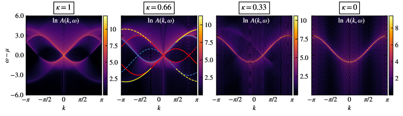
Figure 1: Logarithm of the zero temperature spectral function $\ln A(k,\omega)$ of a TG gas on the lattice for different values of the statistics parameter. The relevant parameters are $L=300$, $N=100$ and $V(j,t\geq 0)=0$. In the second panel the continuous blue, red and yellow lines mark the $\varepsilon_{I}(k)$ , $\varepsilon_{II}(k)$ and $\varepsilon_{III}(k)$ singular lines [see Eqs. (107a), (107b), (107c)] while the corresponding dashed lines describe $-\varepsilon_{I}(k)$ , $-\varepsilon_{II}(k)$ and $-\varepsilon_{III}(k)$.

In this section we are going to investigate the influence of a harmonic trapping potential on the spectral function of a TG gas on the lattice. The spectral function $A(k,\omega)$ defined in (91) quantifies the probability for exciting a particle(hole) with energy $\omega(-\omega)$ and momentum $k$. In general this probability interpretation is not valid in the case of bosonic systems due to the fact that for these systems $A(k,\omega)$ can be negative. However in the case of impenetrable systems of any statistics it can be shown [79] that both contributions on the right hand side of (91) are positive and therefore the probabilistic interpretation is still valid. In Fig. 1 we present the logarithm of the zero temperature spectral function $\ln A(k,\omega)$ for a finite size system with $L=300$ and $N=100$ particles for different values of the statistics parameter and $V(j,t\geq 0)=0$. There are three main singularity lines [74, 79] and below we are going to derive their explicit expressions. We will focus on the bosonic case as the results for different statistics can be obtained by a simple momentum shift with $\kappa(k_{F}-1)$ (see Fig.7 of [59] and the mean field discussion in [79]). For a system of $N$ particles on a lattice with $L$ sites with no external potential and open boundary conditions the single particle dispersion is $\varepsilon(k)=-2J\cos(k)$ with the Fermi vector $k_{F}=\pi N/L$ and the chemical potential given by $-2J\cos k_{F}=\mu$. The first singular line corresponds to the case when a particle is excited from the Fermi level $k_{F}$ to $k_{F}+q$. This particle-type excitation is also present in continuous systems (Type I excitation in Lieb’s classification [80]) and has energy $-2J\cos(k_{F}+q)+2J\cos k_{F}$ and momentum $k=k_{F}+q-k_{F}$. Using the definition of the chemical potential the first singularity line is $\varepsilon_{I}(k)=-2J\cos(k_{F}+k)-\mu$. The second line is due to hole-type excitations (Type II excitations in Lieb’s classification) in which a particle from the Fermi sea with quasimomentum $-k_{F}\leq k\leq k_{F}$ moves to the first unoccupied state above the Fermi level i.e., $k_{F}+\pi/L$. Neglecting $1/L$ corrections, the energy and momentum of these excitations are $-2J\cos k_{F}+2J\cos q$ and $k=k_{F}-q$ respectively. Therefore, the singularity line is give by $\varepsilon_{II}(k)=2J\cos(k_{F}-k)+\mu$. The third line has no equivalent in continuous systems and is generated by excitations from an occupied state inside the Fermi sea $q$ to a state with quasimomentum $\pi-q$. The energy and momenta of these excitations are $-2J\cos(\pi-q)+2J\cos q$ and $k=\pi-2q$ and the line is described by $\varepsilon_{III}(k)=-2J\cos[(\pi+k)/2]+2J\cos[(\pi-k)/2]=4J\sin(k/2)$. The general result valid for any value of the statistics parameter $\kappa$ is obtained by shifting $k\rightarrow k+k_{F}(\kappa-1)$. We find

$$\varepsilon_{I}(k) =-2J\cos(k+k_{F}\kappa)-\mu\,,$$ (107a)

$$\varepsilon_{II}(k) =2J\cos(k+k_{F}\kappa-2k_{F})+\mu\,,$$ (107b)

$$\varepsilon_{III}(k) =4J\sin[(k+k_{F}\kappa-k_{F})/2]\,.$$ (107c)

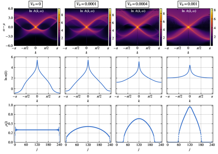
Figure 2: First row: Logarithm of the spectral function $\ln A(k,\omega)$ for a harmonically trapped $(V(j,t\geq 0)=V_{0}\left[j-(L+1)/2\right]^{2})$ bosonic TG gas on the lattice at temperature $T=0.05$ and different values of the curvature $V_{0}$. The other relevant parameters are $L=240$ and $N=80$. The second row present the logarithm of the momentum distribution $\ln n(k)$ and the third row the density of particles $\rho(j)$ on the lattice.

In the case of homogeneous continuous systems the non-linear Luttinger theory [140] predicts that the spectral function has a power-law behaviour $A(k,\omega)\sim|\omega-\varepsilon_{j}(k)|^{-\mu_{j}}$ with $j=\{I,II\}$ near each singular line $\varepsilon_{j}(k)$. The spectral function of a lattice system at small filling fractions presents power law behaviour near the singular lines with power exponents which are very close to the nonlinear Luttinger liquid predictions [74, 79]. From Fig. 1 we see that as the statistics parameter decreases the spectral weight from $\varepsilon_{II}(k)$ and $\varepsilon_{III}(k)$ also decreases being transferred to $\varepsilon_{I}(k)$ which becomes the only singular line at $\kappa=0$ as it is expected for a free fermionic system.

Fig. 2 presents results for the spectral function, momentum distribution and density profile for a system of hard-core bosons $(\kappa=1)$ at temperature $T=0.05$ in the presence of a harmonic trapping potential $V(j,t\geq 0)=V_{0}\left[j-(L+1)/2\right]^{2}$ of different curvatures. The presence of the confining potential has a dramatic effect on both static and dynamic properties of the system. While in the case of open boundary conditions the density is almost constant with small distortions along the boundaries from the last row of Fig. 2 we see that as we increase the strength of the harmonic potential the density profile becomes nonuniform with a large number of particles concentrated in the center of the trap and very few particles at the edges. At a critical value of the curvature (the number of particles is kept constant) the density of the particles in the center of the trap will become one and by further increasing $V_{0}$ this insulating region with zero compressibility will further increase. What we have described is the well known superfluid to Mott insulator quantum phase transition (QPT) [1] induced by the variation of the potential’s curvature. The microscopic origin of this QPT has been investigated in [141]. While in the case of trapped continuum system the energy level spacing of the single particle system is constant, in the lattice case the level spacing decreases with increasing level number until a degeneracy sets in and the level spacing becomes monotonously increasing. The eigenfunctions of the degenerate states have the interesting characteristic of having zero weight in the middle of the trap and as the level increases this region in which the eigenfunctions have zero weight also increases. The QPT occurs when the Fermi energy is close to the level where this degeneracy sets in and the density in the center of the trap approaches one. Further increasing the curvature of the potential results in a similar increase of the insulating region and due to the Pauli principle the eigenfunctions should also have an increasing region with zero weight in the center of the trap as the level increases, which is exactly the phenomenon mentioned above.

Signatures of the QPT can also been seen in the momentum distribution which due to the presence of the lattice is a periodic function in the reciprocal lattice. While in the case of bosons and fermions the momentum distribution $n(k)$ is symmetric with respect to $k=0$ we should point out that for anyonic systems this is no longer valid as a result of the broken space-reversal symmetry of the commutation relations (84). At zero temperature and small values of the curvature there is always a region in which $n(k)=0$ but as we increase $V_{0}$ another way of identifying the presence of the insulating phase is the fact that $n(k=\pm\pi)$ becomes nonzero [141]. As the size of the insulator region increases this is also accompanied by a similar increase of $n(k=\pm\pi)$. At finite but low temperature we can see from the second row of Fig. 2 that we encounter a similar phenomenon. When $V_{0}=0$ the momentum distribution is very close to the usual quasicondensate behaviour at $T=0$ with $n(k)\sim k^{-1/2}$ at $k=0$ and $n(k=\pm\pi)\sim 0$ (this is due to thermal fluctuations). As we increase the strength of the confining potential $n(k=\pm\pi)$ also increases and as an insulating plateau develops we see that $n(k)$ becomes almost flat with a smooth peak at $k=0$.

As the spectral function quantifies the probability that a particle (hole) to be excited (filled) at a given momentum $k$ and energy $\omega$ and the tails of the momentum distribution become more populated with increasing curvature one would expect that the spectral weight would get transferred to the hole component $(\omega\leq\mu)$ of $A(k,\omega)$ as $V_{0}$ increases. This is indeed the case and it can be seen in the first row of Fig. 2. An interesting peculiarity of one dimensional systems is that at low energies the spectral function has a region in which it is zero (or it is very small at finite temperatures). In our case for the homogeneous system at $T=0$ this region is defined by $|\omega-\mu|<\varepsilon_{II}(k)$ and is due to the fact that the Fermi sphere in 1D is comprised of only two points $\pm k_{F}$. While in higher dimensions the hole excitations lead to a continuum extending to zero energy for all momenta $q$ smaller than $2k_{F}$ in 1D the only place where the hole excitations can reach zero are for $q=0$ and $q=2k_{F}$. At moderate values of the curvature, $V_{0}=0.0001$, we see that the region in which the spectral function vanishes for a homogeneous system decreases considerably but as we further increase the curvature the opposite phenomenon occurs. An interesting feature is revealed at $V_{0}=0.0004$ where we can see that $A(k,\omega\leq\mu)$ is almost similar with $A(k,\omega\geq\mu)$ for a homogeneous system ($V_{0}=0$). For $V_{0}=0.001$ and zero temperature the system would develop an insulator region in the middle of the trap. In this case we see from Fig. 2 that the spectral function presents only two singular lines compared with the three in the case of the homogeneous system or for the trapped system before the QPT. Therefore, the measurement of the spectral function would provide an alternative way of identifying the presence of the Mott insulator phase in a trapped 1D system.

VIII Conclusions

We have derived determinant representations for the Green’s functions and spectral function of impenetrable particles of arbitrary statistics on the lattice and in the continuum. Our results are valid at zero and finite temperature and for general confining potentials including nonequlibrium scenarios due to the sudden changes of the external potential. The main advantage of our approach is the numerical efficiency with the main computational cost being the calculation of partial overlaps of the dynamical evolving single particle basis. Our numerical analysis of the spectral function for a trapped TG gas on the lattice showed that the presence of the external potential has a profound effect on the distribution of the spectral weight culminating with the vanishing of one of the spectral lines present in the homogeneous system as we increase the curvature of the potential. In addition, our results also constitute the starting point in the rigorous analysis of the asymptotics of the correlation functions using powerful techniques developed in the last decades [54, 67, 70, 72] and can be used for benchmarking numerical work in the finite coupling case [142, 143]. A natural generalization of our results would be the derivation of similar representations for the correlators of impenetrable multicomponent systems like the Gaudin-Yang and Hubbard models. This will be deferred to a future publication.

Appendix A The equal time case of $g^{(-)}(x,t;y,t^{\prime})$

In this appendix we investigate how the $g^{(-)}(x,t;y,t^{\prime})$ correlator simplifies when $t=t^{\prime}$. In the continuum case we have $\textsf{U}_{a,b}^{(-)}(x,t;y,t)=\sum_{q=1}^{\infty}\overline{f}(a,q|\kappa,x,t)f(b,q|\kappa,y,t)$ with $f(a,q|\kappa,x,t)$ defined in (30). We introduce $\xi=(1-e^{i\pi\kappa})$ and consider first the case $x\leq y$. We have

$$\textsf{U}_{a,b}^{(-)}(x,t;y,t)-\delta_{a,b} =-\overline{\xi}\int_{x}^{L_{+}}\overline{\phi}_{a}(v,t)\phi_{b}(v,t)\,dv-\xi\int_{y}^{L_{+}}\overline{\phi}_{a}(w,t)\phi_{b}(w,t)\,dw$$

$$\qquad\qquad\qquad\qquad+\xi\,\overline{\xi}\sum_{q=1}^{\infty}\left(\int_{x}^{L_{+}}\overline{\phi}_{a}(v,t)\phi_{q}(v,t)\,dv\right)\left(\int_{y}^{L_{+}}\phi_{b}(w,t)\overline{\phi}_{q}(w,t)\,dw\right)\,,$$

$$=-\overline{\xi}\int_{x}^{y}\overline{\phi}_{a}(v,t)\phi_{b}(v,t)\,dv-(\xi+\overline{\xi})\int_{y}^{L_{+}}\overline{\phi}_{a}(w,t)\phi_{b}(w,t)\,dw$$

$$\qquad\qquad\qquad\qquad+\xi\,\overline{\xi}\sum_{q=1}^{\infty}\left(\int_{x}^{y}\overline{\phi}_{a}(v,t)\phi_{q}(v,t)\,dv\right)\left(\int_{y}^{L_{+}}\phi_{b}(w,t)\overline{\phi}_{q}(w,t)\,dw\right)$$

$$\qquad\qquad\qquad\qquad+\xi\,\overline{\xi}\sum_{q=1}^{\infty}\left(\int_{y}^{L_{+}}\overline{\phi}_{a}(v,t)\phi_{q}(v,t)\,dv\right)\left(\int_{y}^{L_{+}}\phi_{b}(w,t)\overline{\phi}_{q}(w,t)\,dw\right)\,.$$ (108)

We will show first that the second term on the right hand sided of (A) cancels the fourth using the completeness of the $\phi_{k}(v)$ functions

$$\int_{L_{-}}^{L_{+}}\overline{\phi}_{a}(v,t)\phi_{b}(v,t)=\delta_{a,b}\,,\ \ \ \sum_{a=1}^{\infty}\overline{\phi}_{a}(x,t)\phi_{a}(y,t)=\delta(x-y)\,.$$ (109)

We introduce $\widetilde{\overline{\phi}}_{a}(v,t)=\mathbf{1}_{[y,L_{+}]}\overline{\phi}_{a}(v,t)$ and $\widetilde{\phi}_{b}(v,t)=\mathbf{1}_{[y,L_{+}]}\phi_{b}(v,t)$ with $\mathbf{1}_{[y,L_{+}]}$ the characteristic function of the interval $[y,L_{+}]$ i.e., is 1 when $v$ is inside the interval and 0 otherwise. We have

$$\int_{y}^{L_{+}}\overline{\phi}_{a}(v,t)\phi_{b}(v,t)\,dv =\int_{L_{-}}^{L_{+}}\widetilde{\overline{\phi}}_{a}(v,t)\widetilde{\phi}_{b}(v,t)\,dv\,,$$

$$=\int_{L_{-}}^{L_{+}}\int_{L_{-}}^{L_{+}}\widetilde{\overline{\phi}}_{a}(v,t)\delta(v-w)\widetilde{\phi}_{b}(w,t)\,dvdw\,,$$

$$=\sum_{q=1}^{\infty}\left(\int_{L_{-}}^{L_{+}}\widetilde{\overline{\phi}}_{a}(v,t)\phi_{q}(v,t)\,dv\right)\left(\int_{L_{-}}^{L_{+}}\overline{\phi}_{q}(w,t)\widetilde{\phi}_{b}(w,t)\,dw\right)\,,$$

$$=\sum_{q=1}^{\infty}\left(\int_{y}^{L_{+}}\overline{\phi}_{a}(v,t)\phi_{q}(v,t)\,dv\right)\left(\int_{y}^{L_{+}}\overline{\phi}_{q}(w,t)\phi_{b}(w,t)\,dw\right)\,.$$ (110)

This relation together with $\xi+\overline{\xi}=\xi\overline{\xi}=2-2\cos\pi\kappa$ shows that the second and the fourth term of (A) cancel. In a similar fashion it can be shown that the third term is zero. Considering $\widetilde{\overline{\phi}}_{a}(v,t)=\mathbf{1}_{[x,y]}\overline{\phi}_{a}(v,t)$ and $\widetilde{\phi}_{b}(v,t)=\mathbf{1}_{[y,L_{+}]}\phi_{a}(v,t)$ we have $\int_{L_{-}}^{L_{+}}\widetilde{\overline{\phi}}_{a}(v,t)\widetilde{\phi}_{b}(v,t)\,dv=0$ and by inserting a resolution of the identity this is identical with the third term on the r.h.s. of (A). Therefore, for $x<y$ we have

$$\textsf{U}_{a,b}^{(-)}(x,t;y,t)-\delta_{a,b}=-\overline{\xi}\int_{x}^{y}\overline{\phi}_{a}(v,t)\phi_{b}(v,t)\,dv\,.$$ (111)

In the case $x>y$ we obtain

$$\textsf{U}_{a,b}^{(-)}(x,t;y,t)-\delta_{a,b}=-\xi\int_{y}^{x}\overline{\phi}_{a}(v,t)\phi_{b}(v,t)\,dv\,.$$ (112)

From (111) and (112) we obtain (104). The result for the lattice case is given by (106).

References

• [1] M. A. Cazalilla, R. Citro, T. Giamarchi, E. Orignac, and M. Rigol, One dimensional bosons: From condensed matter systems to ultracold gases, Rev. Mod. Phys. 83, 1405 (2011).
• [2] X.-W. Guan, M.T. Batchelor, and C. Lee, Fermi gases in one dimension: From Bethe ansatz to experiments, Rev. Mod. Phys. 85, 1633 (2013).
• [3] S.I. Mistakidis, A.G. Volosniev, R.E. Barfknecht, T. Fogarty, Th. Busch, A. Foerster, P. Schmelcher, and N.T. Zinner, Cold atoms in low dimensions – a laboratory for quantum dynamics, arXiv:2202.11071.
• [4] A. Minguzzi and P. Vignolo, Strongly interacting trapped one-dimensional quantum gases: an exact solution, arXiv:2201.02362.
• [5] E.H. Lieb and W. Liniger, Exact Analysis of an Interacting Bose Gas. I. The General Solution and the Ground State, Phys. Rev. 130, 1605 (1963).
• [6] M. Girardeau, Relationship between Systems of Impenetrable Bosons and Fermions in One Dimension, J. Math. Phys. (N.Y.) 1, 516 (1960).
• [7] M. Olshanii, Atomic Scattering in the Presence of an External Confinement and a Gas of Impenetrable Bosons, Phys. Rev. Lett. 81, 938 (1998).
• [8] H. Moritz, T.Stöferle, M. Köhl, and T. Esslinger, Exciting Collective Oscillations in a Trapped 1D Gas, Phys. Rev. Lett. 91, 250402 (2003).
• [9] T. Kinoshita, T. Wenger, and D. S. Weiss, Observation of a One-Dimensional Tonks-Girardeau Gas, Science 305, 1125 (2004).
• [10] B. Paredes, A. Widera, V. Murg, O. Mandel, S. Fölling, I. Cirac, G. V. Shlyapnikov, T. W. Hänsch, and I. Bloch, Tonks-Girardeau gas of ultracold atoms in an optical lattice, Nature (London) 429, 277 (2004).
• [11] E. Lieb, T. Schultz, and D. Mattis, Two soluble models of an antiferromagnetic chain, Ann. Phys. 16, 407 (1961).
• [12] A. Kundu, Exact Solution of Double $\delta$ Function Bose Gas through an Interacting Anyon Gas, Phys. Rev. Lett. 83, 1275 (1999).
• [13] M.T. Batchelor, X.-W. Guan, and N. Oelkers, One-Dimensional Interacting Anyon Gas: Low-Energy Properties and Haldane Exclusion Statistics, Phys. Rev. Lett. 96, 210402 (2006).
• [14] Y. Hao, Y. Zhang, and S.Chen, Ground-state properties of hard-core anyons in one-dimensional optical lattices, Phys. Rev. A 79, 043633 (2009).
• [15] T. Keilmann, S. Lanzmich, I. McCulloch, and M. Roncaglia, Statistically induced phase transitions and anyons in 1D optical lattices, Nat. Commun. 2, 361 (2011).
• [16] M. Bonkhoff, K. Jägering, S. Eggert, A. Pelster, M. Thorwart, and T. Posske, Bosonic Continuum Theory of One-Dimensional Lattice Anyons, Phys. Rev. Lett. 126, 163201 (2021).
• [17] S. Greschner and L. Santos, Anyon Hubbard Model in One-Dimensional Optical Lattices, Phys. Rev. Lett. 115, 053002 (2015).
• [18] C. Sträter, S. C. L. Srivastava, and A. Eckardt, Floquet Realization and Signatures of One-Dimensional Anyons in an Optical Lattice, Phys. Rev. Lett. 117, 205303 (2016).
• [19] L. Cardarelli, S. Greschner, and L. Santos, Engineering interactions and anyon statistics by multicolor lattice depth modulations, Phys. Rev. A 94, 023615 (2016).
• [20] S. Greschner, L. Cardarelli, and L. Santos, Probing the exchange statistics of one-dimensional anyon models, Phys. Rev. A 97, 053605 (2018).
• [21] G.D. Mahan, Many-Particle Physics (Kluwer Academic/Plenum Publishers, New York, 2000).
• [22] A. Damascelli, Probing the Electronic Structure of Complex Systems by ARPES, Phys. Scr. T109, 61 (2004).
• [23] C. Chin, M. Bartenstein, A. Altmeyer, S. Riedl, S. Jochim, J. H. Denschlag, and R. Grimm, Observation of the Pairing Gap in a Strongly Interacting Fermi Gas, Science 305, 1128 (2004).
• [24] V. V. Volchkov, M. Pasek, V. Denechaud, M. Mukhtar, A. Aspect, D. Delande, and V. Josse, Measurement of Spectral Functions of Ultracold Atoms in Disordered Potentials, Phys. Rev. Lett. 120, 060404 (2018).
• [25] J. T. Stewart, J. P. Gaebler, and D. S. Jin, Using photoemission spectroscopy to probe a strongly interacting Fermi gas, Nature (London) 454, 744 (2008).
• [26] T.-L. Dao, I. Carusotto, and A. Georges, Probing quasiparticle states in strongly interacting atomic gases by momentum-resolved Raman photoemission spectroscopy, Phys. Rev. A 80, 023627 (2009).
• [27] G. Veeravalli, E. Kuhnle, P. Dyke, and C. J. Vale, Bragg Spectroscopy of a Strongly Interacting Fermi Gas, Phys. Rev. Lett. 101, 250403 (2008).
• [28] R. Jördens, N. Strohmaier, K. Gunter, H. Moritz, and T. Esslinger, A Mott insulator of fermionic atoms in an optical lattice, Nature (London) 455, 204 (2008).
• [29] D. Greif, L. Tarruell, T. Uehlinger, R. Jördens, and T. Esslinger, Probing Nearest-Neighbor Correlations of Ultracold Fermions in an Optical Lattice, Phys. Rev. Lett. 106, 145302 (2011).
• [30] A. Bohrdt, D. Greif, E. Demler, M. Knap, and F. Grusdt, Angle-resolved photoemission spectroscopy with quantum gas microscopes, Phys. Rev. B 97, 125117 (2018).
• [31] V.I. Yukalov and M.D. Girardeau, Fermi-Bose mapping for one-dimensional Bose gases, Laser Phys. Lett. 2, 375 (2005).
• [32] M.D. Girardeau, Anyon-Fermion Mapping and Applications to Ultracold Gases in Tight Waveguides, Phys. Rev. Lett. 97, 100402 (2006).
• [33] O.I. Pâţu, V.E. Korepin, and D.V. Averin, One-Dimensional Impenetrable Anyons in Thermal Equilibrium. I. Anyonic Generalization of Lenard’s Formula, J. Phys. A 41, 145006 (2008).
• [34] A. Lenard, Momentum Distribution in the Ground State of the One‐Dimensional System of Impenetrable Bosons, J. Math. Phys. (N.Y.) 5, 930 (1964).
• [35] E. Barouch and B.M. McCoy, Statistical mechanics of the XY model. II. Spin-correlation functions, Phys. Rev. A 3, 786 (1971).
• [36] E. Barouch and B.M. McCoy, Statistical mechanics of the XY model. III, Phys. Rev. A 3, 2137 (1971).
• [37] B.M. McCoy, E. Barouch, and D.B. Abraham, Statistical mechanics of the XY model. IV. Time-dependent spin-correlation functions, Phys. Rev. A 4, 2331 (1971).
• [38] R. Santachiara, F. Stauffer, and D. C. Cabra, Entanglement properties and momentum distributions of hard-core anyons on a ring, J. Stat. Mech. L05003 (2007).
• [39] R. Santachiara and P. Calabrese, One-particle density matrix and momentum distribution function of one-dimensional anyon gases, J. Stat. Mech. P06005 (2008).
• [40] T. Papenbrock, Ground-state properties of hard-core bosons in one-dimensional harmonic traps, Phys. Rev. A 67, 041601(R) (2003).
• [41] P.J. Forrester, N.E. Frankel, T.M. Garoni, and N.S. Witte, Finite one-dimensional impenetrable Bose systems: Occupation numbers, Phys. Rev. A 67, 043607 (2003).
• [42] P.J. Forrester, N.E. Frankel, T.M. Garoni, and N.S. Witte, Painlevé transcendent evaluations of finite system density matrices for 1D impenetrable bosons, Commun. Math. Phys. 238, 257 (2003).
• [43] G. Marmorini, M. Pepe, and P. Calabrese, One-body reduced density matrix of trapped impenetrable anyons in one dimension, J. Stat. Mech. 073106 (2016).
• [44] Y. Hao, Ground-state properties of hard-core anyons in a harmonic potential, Phys. Rev. A 93, 063627 (2016).
• [45] Y. Hao and Y. Song, One-dimensional hard-core anyon gas in a harmonic trap at finite temperature, Eur. Phys. J. D 71, 135 (2017).
• [46] T.D. Schultz, Note on the One–Dimensional Gas of Impenetrable Point–Particle Bosons, J. Math. Phys. 4, 666 (1963).
• [47] A. Lenard, One‐Dimensional Impenetrable Bosons in Thermal Equilibrium, J. Math. Phys. (N.Y.) 7, 1268 (1966).
• [48] V.E. Korepin and N.A. Slavnov, The Time Dependent Correlation Function of an Impenetrable Bose Gas as a Fredholm Minor. I, Commun. Math. Phys. 129, 103 (1990).
• [49] O.I. Pâţu, V.E. Korepin, D.V. Averin, One-dimensional impenetrable anyons in thermal equilibrium: II. Determinant representation for the dynamic correlation functions, J. Phys A 41, 255205 (2008).
• [50] F. Colomo, A.G. Izergin, V.E. Korepin, and V. Tognetti, Temperature correlation functions in the XX0 Heisenberg chain. I, Theor. Math. Phys. 94, 11 (1993).
• [51] O.I. Pâţu, Correlation functions and momentum distribution of one-dimensional hard-core anyons in optical lattices, J. Stat. Mech. P01004 (2015).
• [52] F. Göhmann, K.K. Kozlowski, J. Sirker, and J. Suzuki, Equilibrium dynamics of the XX chain, Phys. Rev. B 100, 155428 (2019).
• [53] Y. Zhuravlev, E. Naichuk, N. Iorgov, and O. Gamayun, Large-time and long-distance asymptotics of the thermal correlators of the impenetrable anyonic lattice gas, Phys. Rev. B 105, 085145 (2022).
• [54] V.E. Korepin, N.M. Bogoliubov, and A.G. Izergin, Quantum Inverse Scattering Method and Correlation Functions (Cambridge University Press, Cambridge, UK, 1993).
• [55] A. R. Its, A. G. Izergin, V. E. Korepin, and N. A. Slavnov, Temperature correlations of quantum spins, Phys. Rev. Lett. 70, 1704 (1993).
• [56] A. Berkovich, Temperature and magnetic field-dependent correlators of the exactly integrable (1+1)-dimensional gas of impenetrable fermions, J. Phys. A 24, 1543 (1991).
• [57] F. Göhmann, A.R. Its, and V.E. Korepin, Correlations in the impenetrable electron gas, Phys. Lett. A 249, 117 (1998).
• [58] V.V. Cheianov and M.B. Zvonarev, Zero temperature correlation functions for the impenetrable fermion gas, J. Phys. A 37, 2261 (2004).
• [59] O.I. Pâţu, Correlation functions of one-dimensional strongly interacting two-component gases, Phys. Rev. A 100, 063635 (2019).
• [60] A. Lenard, Some remarks on large Toeplitz determinants, Pacific J. Math 42, 137 (1972).
• [61] A.A. Ovchinnikov, Fisher-Hartwig conjecture and the correlators in XY spin chain, Phys. Lett. A 366, 357 (2007).
• [62] H.G. Vaidya and C.A. Tracy, One-Particle Reduced Density Matrix of Impenetrable Bosons in One Dimension at Zero Temperature, Phys. Rev. Lett. 42, 3 (1979).
• [63] M. Jimbo, T. Miwa, Y. Môri, and M. Sato, Density matrix of an impenetrable Bose gas and the fifth Painlevé transcendent, Physica (Amsterdam) 1D, 80 (1980).
• [64] D.M. Gangardt, Universal correlations of trapped one-dimensional impenetrable bosons, J. Phys. A: Math. Gen. 37, 9335 (2004).
• [65] D.M. Gangardt and G.V. Shlyapnikov, Off-diagonal correlations of lattice impenetrable bosons in one dimension, New J. Phys. 8, 167 (2006).
• [66] P. Calabrese and R. Santachiara, Off-diagonal correlations in one-dimensional anyonic models: A replica approach, J. Stat. Mech. P03002 (2009).
• [67] N. Kitanine, K.K. Kozlowski, J.M. Maillet, N.A. Slavnov, V. Terras, Form factor approach to dynamical correlation functions in critical models, J. Stat. Mech. P09001 (2012).
• [68] K.K. Kozlowski and V. Terras, Long-time and large-distance asymptotic behavior of the current–current correlators in the non-linear Schrödinger model, J. Stat. Mech. P09013 (2011).
• [69] K.K. Kozlowski, Large-distance and long-time asymptotic behavior of the reduced density matrix in the non-linear Schrödinger model, Ann. Henri Poincaré 16 437 (2015).
• [70] F. Göhmann, M. Karbach, A. Klümper, K.K. Kozlowski, and J. Suzuki, Thermal form-factor approach to dynamical correlation functions of integrable lattice models, J. Stat. Mech. 113106 (2017).
• [71] F. Göhmann, K.K. Kozlowski, and J. Suzuki, Long-time large-distance asymptotics of the transverse correlation functions of the XX chain in the spacelike regime, Lett. Math. Phys. 110, 1783 (2020).
• [72] O. Gamayun, N. Iorgov, and Y. Zhuravlev, Effective free fermionic form factors and the XY spin chain, SciPost Phys. 10, 70 (2021).
• [73] D. Chernowitz and O. Gamayun, On the dynamics of free-fermionic tau-functions at finite temperature, SciPost Physics Core 5, 006 (2022).
• [74] J. Settino, N. Lo Gullo, F. Plastina, and A. Minguzzi, Exact Spectral Function of a Tonks-Girardeau Gas in a Lattice,, Phys. Rev. Lett. 126, 065301 (2021).
• [75] R. Pezer and H. Buljan, Momentum Distribution Dynamics of a Tonks-Girardeau Gas: Bragg Reflections of a Quantum Many-Body Wave Packet, Phys. Rev. Lett. 98, 240403 (2007).
• [76] Y. Y. Atas, D. M. Gangardt, I. Bouchoule, and K. V. Kheruntsyan, Exact nonequilibrium dynamics of finite temperature Tonks-Girardeau gases, Phys. Rev. A 95, 043622 (2017).
• [77] O.I. Pâţu, Nonequilibrium dynamics of the anyonic Tonks-Girardeau gas at finite temperature, Phys. Rev. A 102, 043303 (2020).
• [78] Q.-W. Wang, Exact dynamical correlations of nonlocal operators in quadratic open Fermion systems: a characteristic function approach, SciPost Phys. Core 5, 027 (2022)
• [79] Q.-W. Wang, Exact dynamical correlations of hard-core anyons in one-dimensional lattices, Phys. Rev. B 105, 205143 (2022).
• [80] E.H. Lieb, Exact Analysis of an Interacting Bose Gas. II. The Excitation Spectrum, Phys. Rev. 130, 1616 (1963).
• [81] O.I. Pâţu, V.E. Korepin, and D.V. Averin, Correlation Functions of One-Dimensional Lieb-Liniger Anyons, J. Phys. A 40, 14963 (2007).
• [82] F. Franchini, An Introduction to Integrable Techniques for One-Dimensional Quantum Systems, Lecture Notes in Physics 940 (Springer, Heidelberg, 2017).
• [83] T. Kinoshita, T. Wenger, and D. S. Weiss, A quantum Newton’s cradle, Nature (London) 440, 900 (2006).
• [84] M. Rigol, V. Dunjko, and M. Olshanii, Thermalization and its mechanism for generic isolated quantum systems, Nature (London) 452, 854 (2008).
• [85] M. Rigol, V. Dunjko, V. Yurovsky, and M. Olshanii, Relaxation in a Completely Integrable Many-Body Quantum System: An Ab Initio Study of the Dynamics of the Highly Excited States of 1D Lattice Hard-Core Bosons, Phys. Rev. Lett. 98, 050405 (2007).
• [86] M.D. Girardeau and E.M. Wright, Dark Solitons in a One-Dimensional Condensate of Hard Core Bosons, Phys. Rev. Lett. 84, 5691 (2000).
• [87] K.K. Das, M.D. Girardeau, and E.M. Wright, Interference of a Thermal Tonks Gas on a Ring, Phys. Rev. Lett. 89, 170404 (2002).
• [88] G.P. Berman, F. Borgonovi, F.M. Izrailev, and A. Smerzi, Irregular Dynamics in a One-Dimensional Bose System, Phys. Rev. Lett. 92, 030404 (2004).
• [89] A. Minguzzi and D.M. Gangardt, Exact Coherent States of a Harmonically Confined Tonks-Girardeau Gas, Phys. Rev. Lett. 94, 240404 (2005).
• [90] A. del Campo, Fermionization and bosonization of expanding one-dimensional anyonic fluids, Phys. Rev. A 78, 045602 (2008).
• [91] H. Buljan, R. Pezer, and T. Gasenzer, Fermi-Bose transformation for the time-dependent Lieb-Liniger gas, Phys. Rev. Lett. 100, 080406 (2008).
• [92] M. Collura, S. Sotiriadis, and P. Calabrese, Quench dynamics of a Tonks-Girardeau gas released from a harmonic trap, J. Stat. Mech. P09025 (2013).
• [93] M. Kormos, A. Shashi, Y.Z. Chou, J.S. Caux, and A. Imambekov, Interaction quenches in the one-dimensional Bose gas, Phys. Rev. B 88, 205131 (2013).
• [94] M. Kormos, M. Collura, and P. Calabrese, Analytic results for a quantum quench from free to hard-core one-dimensional bosons, Phys. Rev. A 89, 013609 (2014).
• [95] T.M. Wright, M. Rigol, M.J. Davis, and K.V. Kheruntsyan, Nonequilibrium Dynamics of One-Dimensional Hard-Core Anyons Following a Quench: Complete Relaxation of One-Body Observables, Phys. Rev. Lett. 113, 050601 (2014).
• [96] J. De Nardis, B. Wouters, M. Brockmann, and J.S. Caux, Solution for an interaction quench in the Lieb-Liniger Bose gas, Phys. Rev. A 89, 033601 (2014).
• [97] J. De Nardis and J.S. Caux, Analytical expression for a post-quench time evolution of the one-body density matrix of one-dimensional hard-core bosons, J. Stat. Mech. P12012 (2014).
• [98] A. S. Campbell, D. M. Gangardt, and K. V. Kheruntsyan, Sudden Expansion of a One-Dimensional Bose Gas from Power-Law Traps, Phys. Rev. Lett. 114, 125302 (2015).
• [99] R. van den Berg, B. Wouters, S. Eliëns, J. De Nardis, R. M. Konik, and J.-S. Caux, Separation of Time Scales in a Quantum Newton’s Cradle, Phys. Rev. Lett. 116, 225302 (2016).
• [100] A. Bastianello, M. Collura, and S. Sotiriadis, Quenches from bosonic Gaussian initial states to the Tonks-Girardeau limit: Stationary states and effects of a confining potential, Phys. Rev. B 95, 174303 (2017).
• [101] R. Boumaza and K. Bencheikh, Analytical results for the time-dependent current density distribution of expanding ultracold gases after a sudden change of the confining potential, J. Phys. A 50, 505003 (2017).
• [102] T. Fogarty, A. Usui, T. Busch, A. Silva, and J. Goold, Dynamical phase transitions and temporal orthogonality in one-dimensional hard-core bosons: from the continuum to the lattice, New J. Phys. 19, 113018 (2017).
• [103] M. Mikkelsen, T. Fogarty, and T. Busch, Static and dynamic phases of a Tonks–Girardeau gas in an optical lattice, New J. Phys. 20, 113011 (2018).
• [104] J.S. Caux, B. Doyon, J. Dubail, R. Konik, and T Yoshimura, Hydrodynamics of the interacting Bose gas in the Quantum Newton Cradle setup, SciPost Phys. 6, 070 (2019).
• [105] M. Schemmer, I. Bouchoule, B. Doyon, and J. Dubail, Generalized hydrodynamics on an atom chip, Phys. Rev. Lett. 122, 090601 (2019).
• [106] P. Ruggiero, Y. Brun, and J. Dubail, Conformal field theory on top of a breathing one-dimensional gas of hard core bosons, SciPost Physics 6, 051 (2019).
• [107] S. Sotiriadis, Non-Equilibrium Steady State of the Lieb-Liniger model: exact treatment of the Tonks Girardeau limit, arXiv:2007.12683.
• [108] A. Bastianello, A. De Luca, B. Doyon, J. De Nardis, Thermalization of a trapped one-dimensional Bose gas via diffusion, Phys. Rev. Lett. 125, 240604 (2020).
• [109] E. Granet and F.H.L. Essler, A systematic $1/c$-expansion of form factor sums for dynamical correlations in the Lieb-Liniger model, SciPost Phys. 9, 082 (2020).
• [110] E. Granet and F.H.L. Essler, Systematic strong coupling expansion for out-of-equilibrium dynamics in the Lieb-Liniger model, SciPost Phys. 11, 068 (2021).
• [111] Y.Y. Atas, A. Safavi-Naini, and K.V. Kheruntsyan, Nonequilibrium quantum thermodynamics of determinantal many-body systems: Application to the Tonks-Girardeau and ideal Fermi gases, Phys. Rev. A 102, 043312 (2020).
• [112] P. Devillard, D. Chevallier, P. Vignolo, and M. Albert, Full counting statistics of the momentum occupation numbers of the Tonks-Girardeau gas, Phys. Rev. A 101, 063604 (2020).
• [113] I. Bouchoule, B. Doyon, and J. Dubail, The effect of atom losses on the distribution of rapidities in the one-dimensional Bose gas, SciPost Phys. 9, 044 (2020).
• [114] A. Hutsalyuk and B. Pozsgay, Integrability breaking in the one-dimensional Bose gas: Atomic losses and energy loss, Phys. Rev. E 103, 042121 (2021).
• [115] J.M. Wilson, N. Malvania, Y. Le, Y. Zhang, M. Rigol, and D.S. Weiss, Observation of dynamical fermionization, Science 367, 1461 (2020).
• [116] N. Malvania, Y. Zhang, Y. Le, J. Dubail, M. Rigol, and D.S. Weiss, Generalized hydrodynamics in strongly interacting 1D Bose gases, Science 373, 1129 (2021).
• [117] O. Valée and M. Soares, Airy Functions and Applications to Physics (Imperial College Press, London, 2010).
• [118] H. von Koch, Sur les déterminants infinis et les équations différentielles linéaires, Acta Math. 16, 217 (1892).
• [119] G.G. Batrouni, V. Rousseau, R.T. Scalettar, M. Rigol, A. Muramatsu, P.J.H. Denteneer, and M. Troyer, Mott Domains of Bosons Confined on Optical Lattices, Phys. Rev. Lett. 89, 117203 (2002).
• [120] M. Rigol and A. Muramatsu, Emergence of quasicondensates of hard-core bosons at finite momentum, Phys. Rev. Lett. 93, 230404 (2004).
• [121] L. Vidmar, J.P. Ronzheimer, M. Schreiber, S. Braun, S.S. Hodgman, S. Langer, F. Heidrich-Meisner, I. Bloch, and U. Schneider, Dynamical Quasicondensation of Hard-Core Bosons at Finite Momenta, Phys. Rev. Lett. 115, 175301 (2015).
• [122] E. Barouch, B.M. McCoy, and M. Dresden, Statistical mechanics of the XY model. I Phys. Rev. A 2, 1075 (1970).
• [123] T. Antal, Z. Rácz, A. Rákos, and G. M. Schütz, Transport in the XX chain at zero temperature: Emergence of flat magnetization profiles, Phys. Rev. E 59, 4912 (1999).
• [124] M. Rigol and A. Muramatsu, Universal properties of hard-core bosons confined on one-dimensional lattices, Phys. Rev. A 70, 031603 (2004).
• [125] M. Rigol, Finite-temperature properties of hard-core bosons confined on one-dimensional optical lattices, Phys. Rev. A 72, 063607 (2005).
• [126] M. Rigol and A. Muramatsu, Fermionization in an Expanding 1D Gas of Hard-Core Bosons, Phys. Rev. Lett. 94, 240403 (2005).
• [127] M. Rigol and A. Muramatsu, Nonequilibrium dynamics of Tonks-Girardeau gases on optical lattices, Laser Phys. 16, 348 (2006).
• [128] M. Rigol, A. Muramatsu, and M. Olshanii, Hard-core bosons on optical superlattices: Dynamics and relaxation in the superfluid and insulating regimes, Phys. Rev. A 74, 053616 (2006).
• [129] T. Platini and D. Karevski, Relaxation in the XX quantum chain, J. Phys. A 40, 1711 (2007).
• [130] Y. Hao and S. Chen, Dynamical properties of hard-core anyons in one-dimensional optical lattices, Phys. Rev. A 86, 043631 (2012).
• [131] L. Vidmar, W. Xu, and M. Rigol, Emergent eigenstate solution and emergent Gibbs ensemble for expansion dynamics in optical lattices, Phys. Rev. A 96, 013608 (2017).
• [132] W. Xu and M. Rigol, Expansion of one-dimensional lattice hard-core bosons at finite temperature, Phys. Rev. A 95, 033617 (2017).
• [133] M. Ljubotina, S. Sotiriadis, and T. Prosen, Non-equilibrium quantum transport in presence of a defect: the non-interacting case, SciPost Phys. 6, 004 (2019).
• [134] O. Gamayun, O. Lychkovskiy, and J.-S. Caux, Fredholm determinants, full counting statistics and Loschmidt echo for domain wall profiles in one-dimensional free fermionic chains, SciPost Phys. 8, 036 (2020).
• [135] S. Scopa, A. Krajenbrink, P. Calabrese, and J. Dubail, Exact entanglement growth of a one-dimensional hard-core quantum gas during a free expansion, J. Phys. A 54, 404002 (2021).
• [136] F. Ares, S. Scopa, and S. Wald, Entanglement dynamics of a hard-core quantum gas during a Joule expansion, J. Phys. A 55, 375301 (2022).
• [137] E. Granet, H. Dreyer, and F.H.L. Essler, Out-of-equilibrium dynamics of the XY spin chain from form factor expansion, SciPost Phys. 12, 019 (2022).
• [138] M. Marcus, Determinants of Sums, Coll. Math. J. 21, 130 (1990).
• [139] N. Nessi and A. Iucci, Finite-temperature properties of one-dimensional hard-core bosons in a quasiperiodic optical lattice, Phys. Rev. A 84, 063614 (2011).
• [140] A. Imambekov, T.L. Schmidt, and L.I. Glazman, One-dimensional quantum liquids: Beyond the Luttinger liquid paradigm, Rev. Mod. Phys. 84, 1253 (2012).
• [141] M. Rigol and A. Muramatsu, Confinement control by optical lattices, Phys. Rev. A 70, 043627 (2004).
• [142] M. Panfil and J.-S. Caux, Finite temperature correlations in the Lieb-Liniger 1D Bose gas, Phys. Rev. A 89, 033605 (2014).
• [143] M. Panfil and F.T. Sant’Ana, The relevant excitations for the one-body function in the Lieb-Liniger model, J. Stat. Mech. 073103 (2021).