Hydrogen atom confined inside an inverted-Gaussian potential

Abstract

In this work, we consider the hydrogen atom confined inside a penetrable spherical potential. The confining potential is described by an inverted-Gaussian function of depth $\omega_{0}$, width $\sigma$ and centered at $r_{c}$. In particular, this model has been used to study atoms inside a $C_{60}$ fullerene. For the lowest values of angular momentum $l=0,1,2$, the spectra of the system as a function of the parameters ($\omega_{0},\sigma,r_{c}$) is calculated using three distinct numerical methods: (i) Lagrange-mesh method, (ii) fourth order finite differences and (iii) the finite element method. Concrete results with not less than 11 significant figures are displayed. Also, within the Lagrange-mesh approach the corresponding eigenfunctions and the expectation value of $r$ for the first six states of $s,p$ and $d$ symmetries, respectively, are presented. Our accurate energies are taken as initial data to train an artificial neural network as well. It generates an efficient numerical interpolation. The present numerical results improve and extend those reported in the literature.

I Introduction

In the majority of problems the time-independent Schrödinger equation does not admit exact solutions in terms of elementary functions or in terms of special functions. In such cases it is necessary to solve this equation by means of numerical and approximate methods which inherently carry a certain degree of accuracy. Some of the most common numerical methods are the following: the Numerov method, the spline-based method, the finite difference, the finite element, the Lagrange mesh method and the variational one, among others.

These numerical schemes are widely used in the study of both spatially confined and unconfined quantum systems. In particular, the investigation of spatially confined quantum systems has gained much interest because some of their physical properties change abruptly with the size of the confining barrier. Furthermore, many physical phenomena can be modeled by a confined quantum system as for example: atoms and molecules subject to high external pressures, atoms and molecules in fullerenes, inside cavities such as zeolite molecular sieves or in solvent environments, the specific heat of a crystalline solid under high pressure, etc. A complete list of applications can be found in the articles and reviews on the subject Michels et al. (1937) - Sen and Sen (2014).

Eighty-five years ago, Michels et. al. Michels et al. (1937) calculated the variation of the polarizability of hydrogen under high pressure. To this end, they proposed a simple model of the confined hydrogen atom where, to a first approximation, the nucleus is anchored in the center of a spherical box of radius $r_{0}$ and impenetrable walls. It is assumed that this infinite potential is due to the presence of neighboring negative electric charges. The corresponding wave function vanishes at the surface of the sphere, i. e. it must obey Dirichlet boundary conditions. Since then, this model has been successfully applied in the study of confined many-electron atoms and molecules. However, it takes into account the effects of repulsive forces only. A more realistic potential that embodies an attractive force considers a softer confinement in cavities of penetrable walls. The simplest penetrable confining potential of this type is that of a step potential Ley-Koo and Rubinstein (1979)-Aquino et al. (2018). Some other relevant penetrable confining potentials are the logistic potential Aquino et al. (2013) and the inverted Gaussian function Xie (2010)-Adamowski et al. (2000). Moreover, there are several potentials that have been employed to describe atoms inside fullerenes: the attractive spherical Shell Connerade et al. (2000a), the $\delta$-potential Amusia et al. (1998) and a Gaussian spherical Shell Nascimento et al. (2010).

In this work we calculate the energies and wave functions of the lowest states of a hydrogen atom confined inside a spherical penetrable box. This system has been analyzed in Nascimento et al. (2010) (and references therein). Here, a more accurate and systematic study is carried out. The corresponding confining potential is described by an inverted Gaussian function. To solve the Schrödinger equation we employ three different numerical methods: the Lagrange mesh, finite difference and finite element. They are complemented by the use of an artificial neural network. Making a comparison of the so obtained results we discuss the advantages of each individual method.

II Methodology

The Schrödinger equation of hydrogen atom confined in a Gaussian spherical shell $w(r)$, in atomic units $(\hbar=m_{e}=e=1)$, is of the form

$$\bigg{[}\,-\frac{1}{2}\Delta\ -\ \frac{1}{r}\ +\ w(r)\,\bigg{]}\,\psi\ =\ E\,\psi\ ,$$ (1)

where $\Delta$ is the 3-dimensional Laplacian, and the Gaussian spherical barrier $w(r)$ is given by

$$w(r)\ =\ -\,\omega_{0}\,\textrm{exp}[-(r-r_{c})^{2}/\sigma^{2}]\,,$$ (2)

here, $\omega_{0}$ is the well depth, $r_{c}$ is the position of the center of the peak and $\sigma$ is the width of the Gaussian, respectively. In concrete calculations, for the purposes of comparison with the existing results in the literature, from time to time the parameters $r_{c}$ and $\sigma$ will be presented in Angstroms (Å).

As it is usual for any central potential, the angular momentum is conserved and the solutions of the Schrödinger equation (1) in spherical coordinates ($r,\theta,\phi$) can be factorized, explicitly

$$\psi_{nlm}(r,\theta,\phi)\ =\ R_{nl}(r)\,Y_{l,m}(\theta,\phi)\ ,$$ (3)

with $Y_{l,m}(\theta,\phi)$ being a spherical harmonic function. It is convenient to introduce an auxiliary function $u_{nl}(r)$ defined by the relation $R_{nl}(r)\ =u_{nl}(r)/r$. In this case, from (1) and (3) it follows that $u_{nl}(r)$ must obey the isospectral radial problem

$$\bigg{[}\,-\frac{1}{2}\frac{d^{2}}{dr^{2}}\ +\ V_{\rm eff}(r)\,\bigg{]}u_{nl}(r)\ =\ E\,u_{nl}(r)\ ,$$ (4)

with the boundary condition $u_{nl}(r=0)=0$. The effective potential appearing in (4) is given by

$$V_{\rm eff}(r)\ =\ -\frac{1}{r}\ +\ \frac{l(l+1)}{2\,r^{2}}\ +\ w(r)\ ,$$ (5)

$l=0,1,2,\ldots,$ is the quantum number of angular momentum. Formally, (4) describes a one-dimensional particle of unit mass in the half positive line with an effective potential $V_{\rm eff}(r)$ which is displayed in Figure 1 for fixed $l=0$, $\omega_{0}=1$ a.u., $\sigma=0.5$ a.u. and four different values of $r_{c}$ (the position of the center of the peak). In turn, Figure 2 shows the behavior of $V_{\rm eff}$ (5) as a function of the width $\sigma$ of the Gaussian for fixed $\omega=0.5$ a.u. and $r_{c}=3.54$ Å.

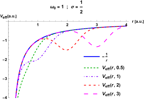
Figure 1: Effective potential $V_{\rm eff}(r,\,r_{c})$ (5) at $l=0$ for $\omega_{0}=1$ a.u., $\sigma=0.5$ a.u. and four different values in a.u. of $r_{c}=0.5,1,2$ and $3$.

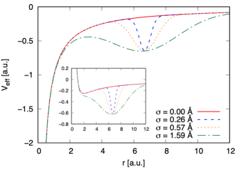
Figure 2: Effective potential $V_{\rm eff}(r)$ (5) with $\omega_{0}=0.5$ a.u. and $r_{c}=3.54$ Å for different $\sigma$ values: $\sigma=0$ (continuous red line), $\sigma=0.25$ Å (blue dashed line), $\sigma=0.57$ Å (orange dotted line) and $\sigma=1.59$ Å (green dash-dotted line). The main figure corresponds to the case of $l=0$ while $l=1$ is shown in the inset.

In order to solve the radial Schrödinger equation (4), three different methods will be employed: $i$) The Lagrange-mesh method, $ii$) Finite difference method, and $iii$) Finite element method. By combining our accurate results with an artificial neural network, we construct an efficient numerical interpolation for the energies.

II.1 The Lagrange-Mesh Method

In the context of the Lagrange-mesh method (LMM) Baye1 and Heenen (1986); Baye (2015), a set of $N$ Lagrange functions $f_{i}\,(x)$ defined over the domain of the radial variable is associated with $N$ mesh points $x_{i}$ which correspond to the zeros of Laguerre polynomials of degree $N$, i.e. $L_{N}(x_{i})=0$. The Lagrange-Laguerre functions $f_{i}\,(x)$ which satisfy the Lagrange conditions

$$f_{i}(x_{j})=\lambda_{i}^{-1/2}\delta_{ij}\,,$$ (6)

at the $N$ mesh points are given by

$$f_{i}(x)=(-1)^{i}\frac{x}{x_{i}^{1/2}}\frac{L_{N}(x)}{(x-x_{i})}e^{-x/2}\,.$$ (7)

The coefficients $\lambda_{i}$ are the weights associated with a Gauss quadrature

$$\int_{0}^{\infty}G(x)dx\approx\sum_{k=1}^{N}\lambda_{k}\,G(x_{k})\,.$$ (8)

In terms of the $N$ Lagrange functions $f_{i}(x)$ (7), the solution of the Schrödinger equation (4) is expressed as

$$\psi(r)=\sum_{i=1}^{N}c_{i}f_{i}(r)\,.$$ (9)

The trial function (9), together with the Gauss quadrature (8) and the Lagrange conditions (6) leads to the system of variational equations

$$\sum_{j=1}^{N}\left[h^{-2}\,T_{ij}+\left(\frac{l(l+1)}{2\,h^{2}\,x_{i}^{2}}-\frac{1}{h\,x_{i}}+\omega(h\,x_{i})\right)\delta_{ij}\right]\,c_{j}=E\,c_{i}\,,$$ (10)

where $\omega(x_{i})$ is the Gaussian potential (2) evaluated at the mesh points $x_{i}$ and $T_{ij}$ are the kinetic-energy matrix elements whose explicit expression is found in Baye (2015). $h$ is a scaling factor that allows to adjust the mesh to the system in consideration. By solving the system (10), not only the energies $E$ are obtained but also the eigenvectors $c_{i}$ from which the approximation to the wave function (9) is obtained.

Inside of the LMM approach, the expectation value of the radial coordinate $r$ is easily calculated. Given the approximation to the wave function (9) together with Gauss quadrature (8) and the Lagrange condition (6) leads to

$$\langle r\rangle=\sum_{i=1}^{N}c_{i}^{2}\,x_{i}\,,$$ (11)

where $c_{i}$ are the eigenvectors resulting from solving (9) and $x_{i}$ are the mesh points.

II.2 Finite difference method

The finite difference method (FDM) is a numerical method easy to implement on a computer, and it is used to solve ordinary and partial differential equations in an approximate way. The method is based on the discretization of the Hamiltonian on a spatial grid, replacing the values of the function and its derivatives by their values at discrete points. The Schrödinger equation is then solved on a uniform grid Kobus (1993) defined by the set of discrete points which are the nodal points $\left\{r_{j}\right\}$.

In order to use the finite difference method and the finite element method, it is convenient to encase the system inside a spherical box with impenetrable walls of radius $r_{\max}$. In this case, the Schrödinger equation to be solved can be written as (cf. (4)):

$$-\frac{1}{2}\frac{d^{2}\tilde{u}_{nl}}{dr^{2}}\,+\,V_{\rm eff}(r)\,\tilde{u}_{nl}\,+\,V_{c}\,\tilde{u}_{nl}\,=\,E_{\max}\,\tilde{u}_{nl},$$ (12)

where $V_{\rm eff}(r)$ is the effective potential (5) and the confinement potential $V_{c}$ is defined as follows

$$V_{c}(r)=\left\{\begin{tabular}[]{l}0\ , \qquad\, if $\ r\leq r_{\max}$\\ $\infty\ ,$ \qquad if $\ r>r_{\max}$\end{tabular}\right.$$ (13)

In the region $r<r_{\max}$ the Schrödinger equation becomes

$$-\frac{1}{2}\frac{d^{2}\tilde{u}_{nl}}{dr^{2}}\ +\ V_{\rm eff}(r)\ \tilde{u}_{nl}\ =\ E_{\max}\,\tilde{u}_{nl}\,.$$ (14)

This differential equation (14) will be solved by the finite difference and finite element methods. The function $\tilde{u}$ satisfies the Dirichlet boundary conditions:

$$\tilde{u}_{nl}(0)\ =\ 0\ ,$$ (15)

$$\tilde{u}_{nl}(r_{\max})\ =\ 0\ .$$

The original energy eigenvalues and eigenfunctions of the free (unbounded) system (4) are recovered in the limit $r_{\max}\rightarrow\infty$,

$$\tilde{u}_{nl}(r)\,\rightarrow\,u_{nl}(r)\,,\qquad E_{\max}\,\rightarrow\,E\ .$$ (16)

As was mentioned above, to find the solution of the radial Schrödinger equation (14) in the region $\left[0,r_{\max}\right]$, the domain is splitted in $N$ subintervals of equal length $h$:

$$0=r_{1}<r_{2}<\cdot\cdot\cdot<r_{N+1}=r_{\max},$$ (17)

where $h=r_{j+1}-r_{j}$.

Now, a second order centred difference approximation to the second derivative can be used, namely

$$\tilde{u}^{{}^{\prime\prime}}\ =\ \frac{\tilde{u}(r_{j+1})-2\tilde{u}(r_{j})+\tilde{u}(r_{j-1})}{h^{2}}\ +\ O(h^{2})\ .$$ (18)

Hence, the Schrödinger equation can be written as an eigenvalue problem $H\,C\,=\,E\,C$ where the matrix $H$ is a tridiagonal matrix whose elements different of zero are given by:

$$H_{ij} = \frac{1}{h^{2}}+V_{\rm eff}(r_{i})\ ,$$ (19)

$$H_{i,i+1} = -\frac{1}{2h^{2}}\ ,$$

$$H_{i,i-1} = -\frac{1}{2h^{2}}\ .$$

whereas the vector $C$ contains the values of $\tilde{u}$ evaluated on the grid $C_{i}=\tilde{u}(r_{i}).$

To improve the accuracy of the calculation one can use a forth order centred difference approximation to the second derivative.

II.3 Finite element method

The finite element method (FEM) is a method based on the discretization of the space in elements and the use of polynomial interpolating functions on each element. This method is widely used in engineering, classical physics and quantum mechanics problems, among others. The discretization is based on the reformulation of the differential equation as an equivalent variational problem. The Garlekin methods are employed in the corresponding minimization D. W. Pepper (2017). Usually, one can identify the following steps to solve the associated differential equation: $i)$ to present the problem in a variational formulation, $ii$) a discretization of the domain using FEM, and finally, $iii$) to find the solution of the discrete problem, which may consist of the solution of a system of simultaneous equations or an eigenvalue problem.

In Quantum Mechanics the FEM was used from a few year ago Kobus (1993), M. Friedman and Thieberger (1978), M. Friedman and Thieberger (1979), L. R. Ram-Mohan and Shetzer (1990), Ram-Mohan (2003), Guimarães and Prudente (2005), Moritz (2014). An excellent introduction of FEM in Quantum Mechanics is found in the Ram-Mohan’s book Ram-Mohan (2003). Only the key points of the method will be presented here.

The time independent Schrödinger equation for a particle of mass $m$ subjected to a potential energy $V({\mathbf{r}})$ is given by:

$$\bigg{[}\,-\frac{\hbar^{2}}{2\,m}\Delta\ +\ V({\mathbf{r}})\,\bigg{]}\,\psi({\mathbf{r}})\ =\ E\,\psi({\mathbf{r}})\ .$$ (20)

This equation can be obtained as an extreme value of the following action integral $I$:

$$I=\int d^{3}r\left[\frac{\hbar^{2}}{2m}\nabla\psi^{\ast}\cdot\nabla\psi+\psi^{\ast}\left(\,V\,-\,E\,\right)\psi\right]\ ,$$ (21)

where $\psi^{\ast}$ and $\psi$ are considered as two independent ”fields”. It is assumed that $\psi$ is continuous up to its second derivative. By varying the action $I$ with respect to $\psi^{\ast}$ we obtain the Schrödinger equation (20). In the present problem only the dynamics of the $r$ coordinate is not trivial. The problem is completely analogous to the one-dimensional case in the $r$-space, the variable $r$ varies in the interval $\left[0,r_{\max}\right]$. Hence, the action integral $I$ (in atomic units) is reduced to:

$$I=\int_{0}^{r_{\max}}dr\left\{\frac{1}{2}\frac{d\psi^{\ast}}{dr}\frac{d\psi}{dr}+\psi^{\ast}\left[V_{\rm eff}(r)-E\right]\psi\right\}\ ,$$ (22)

where $\psi=\psi(r)$, and $V_{\rm eff}(r)$ is an effective potential $V_{\rm eff}(r)=V(r)+\frac{l\,(l+1)}{2\,r^{2}}$, c.f. (5).

Now, the interval $\left[0,r_{\max}\right]$ is divided into small subintervals called elements. The action integral (22) can be decomposed as the sum of the action computed in each element,

$$I\ =\ \sum_{j=1}^{n}I^{(j)}\ ,$$ (23)

where $n$ is the number of elements and $I^{(j)}$ is the action integral evaluated on the $jth$ element. Explicitly, the wave function $\psi_{j}$ defined in the $jth$ element is expanded as a linear combination

$$\psi_{j}(r)\ =\ \sum_{j=1}^{n}c_{j}\,N_{j}(r)\ ,$$ (24)

where $c_{j}$, $j=1,2,\ldots,n$, are unknown coefficients to be determined whereas $N_{j}(r)$ are interpolating polynomials. These are defined for the $jth$ element and they are identically zero out of this element.

The basic idea is to make the variation of the action integral with respect to the coefficients $c_{i}^{\ast}$,

$$\frac{\delta I}{\delta c_{i}^{\ast}}\ =\ 0\ ,\quad i=1,2,\ldots,n\ ,$$ (25)

and by solving these equations to obtain the optimal energies and eigenfunctions.

In particular, Guimaraes and Prudente Guimarães and Prudente (2005) developed an alternative version of FEM called p-Finite Element Method (pFEM) to study the confined hydrogen atom, and Nascimento et. al. Nascimento et al. (2010) employed a pFEM version to study the electron structure of endohedrally confined atoms using an attractive gaussian potential to model atoms inside fullerenes.

As $r_{\max}$ becomes very large the energies of a confined system approach those of the confinement-free system. In practice, a large value of both $r_{\max}$ and the parameter $n$, and a polynomial degree for the $N_{j}(r)$ appearing in (24) are chosen and then, the generalized eigenvalue problem is solved. For a fixed $r_{\rm max}$, by increasing either the value of $n$ or the polynomial degree, or both, a higher precision in the results can be achieved as we will explain in the next section.

II.4 Artificial neural networks

Artificial intelligence has emerged as a collection of computational techniques which seek to mimic the human brain in order to complete tasks for which standard algorithms lead to partially satisfactory results or are costly to implement Jackson (2019); You et al. (2020); Lollie et al. (2022); Bhusal et al. (2022). Particularly, neural networks are artificial intelligence algorithms inspired by the workings of neurons in the human brain. These algorithms have demonstrated the capacity of pinpointing relevant specific pieces of information ‘buried’ in huge data sets and unveiling complex non-linear relationships between the inputs and target, which would be all but impossible to accomplish through a standard visual inspection Murdoch and Detsky (2013); Quiroz-Juárez et al. (2021); Villegas et al. (2022).

In this work, we implement a neural network to estimate the eigenvalues of the radial Schrödinger equation (4) for different positions of the peak of the Gaussian, $r_{c}$. This neural network consists of a hidden layer and an output layer under a feed-forward architecture. In general, the output of each neuron before the activation function reads,

$$z=\sum_{i=1}^{N}\omega_{i}x_{i},$$ (26)

where $\omega_{i}$ are the synaptic weights, $x_{i}$ are the inputs, and $N$ is the number of inputs. Importantly, all the neurons in the output layer contain linear activation functions whereas the neurons in the hidden layer have sigmoid functions given by

$$\alpha(z)=\frac{1}{1+e^{-z}}.$$ (27)

Synaptic weights of the neural network are optimized with Levenberg-Marquardt backpropagation method in a direction that minimizes the mean squared error Marquardt (1963); Hagan and Menhaj (1994). This method approaches second-order training speed without having to compute the Hessian matrix. Because the performance function is given by a sum of squares then the Hessian matrix can be approximated as $\mathbf{H}=\mathbf{J}^{T}\mathbf{J}$, where $\mathbf{J}$ is the Jacobian matrix. Using this approximation, the synaptic weights can be updated by the following expression,

$$\mathbf{\omega}_{k+1}=\mathbf{\omega}_{k}-[\mathbf{H}+\mu I]^{-1}\mathbf{J}^{T}\mathbf{e}$$ (28)

where $k$ denotes the $k$th iteration, $\mu$ is the learning rate and $\mathbf{e}$ is the vector of networks errors. To train the neural network, we use a subset of the dataset that contains eigenvalues of the radial Schrödinger equation (4) for different positions $r_{c}$ of the peak of the Gaussian. These eigenvalues are calculated by the Lagrange-mesh method. After the training stage, the neural network is able to predict the eigenvalues of the whole dataset with a coincidence in six significant digits at least.

III Results and discussion

For the hydrogen atom in the presence of a Gaussian confining spherical shell, the energies, eigenfunctions and expectation values of $r$ for the first six states of $s,p$ and $d$ symmetries are accurately calculated. In order to be able to compare with previous results, the values of the parameters of the Gaussian potential (1) that we consider in detail are: $\omega_{0}=0.5$ a.u., $r_{c}=2.5$ Å and $3.54$ Å and $\sigma=0.26,0.57$ and $1.59$ Å. The corresponding results are shown in Tables 1, 2 and 3.

Before discussing these results let us briefly mention some details about the Lagrange-mesh method. In the system (10), there are two free parameters: the size of the mesh $N$ and the scaling factor $h$. The optimal values of this two parameters depend on the considered state of the system as well as on the value of the parameters occurring in the Gaussian potential. In general, the results presented in Tables 1, 2 and 3 for states $s$, $p$ and $d$, respectively, are obtained with a mesh of at least $N=250$ points and $h$ in some interval between $h\in[0.02-1.0]$. The convergence of the LMM is determined by the stability of the results with respect to an increase in the size of the base $N$ and the variation of $h$. Table 1 presents the results for the $1s,\dots,6s$ states. For $r_{c}=3.54$ Å a comparison with Lin and Ho (2012) is possible for the levels $1s$, $2s$, $3s$, $4s$ with $\sigma=1.59,0.57$ and $0.26$ Å where it can be seen a complete agreement in 7 decimal digits (for $1s$ and $2s$ states) and 8 decimal digits (for $3s$ and $4s$). For completeness, the case $\sigma=0$ (the free hydrogen atom) is also presented. For all these $s$-states, the energy decreases by increasing the value of $\sigma$ as can be seen in Figure 3c. On the other hand, the presence of the Gaussian potential has an important effect on the expectation value of $r$ as indicated in the seventh column of Table 1 (see also Figure 3d): $i$) as a function of $\sigma\in[0.00,1.59]$ Å, $\langle r\rangle$ increases for the ground state, whilst $ii$) for the states $4s,\dots,6s$, $\langle r\rangle$ decreases. Columns 3 and 4 of Table 1 (see also Figures 3a and 3b) present the results of the energy and the expectation value $\langle r\rangle$ when the center of the Gaussian potential is $r_{c}=2.50$ Å. As well as for $r_{c}=3.55$ Å, the energy decreases as a function of $\sigma$. The behaviour of the expectation value $\langle r\rangle$ is depicted in Figure 3b. This effect on $\langle r\rangle$ reflects how the electronic charge is attracted to the Gaussian part of the potential.

States with $l=1$ ($2p,\dots,7p$) are presented in Table 2 for $r_{c}=2.50$ and $3.54$ Å. In both cases, the system gets more bound as the value of $\sigma$ increases (see Figures 4a and 4c). For $r_{c}=3.54$ Å a comparison with Lin and Ho (2012) is also possible: we see a complete agreement in 7 decimal digits for the $2p$ state and 8 decimal digits for the $3p$ and $4p$ states for the three values of $\sigma=0.26,0.57$ and $1.59$ Å. The expectation value $\langle r\rangle$ is shown in Figures 4b and 4d.

Results of the energy and the expectation value for $l=2$ ($3d,\dots,8d$) are displayed in Table 3 for $r_{c}=2.50$ and $3.54$ Å. For both values of $r_{c}$, by increasing $\sigma$ the energy becomes more negative. The expectation value $\langle r\rangle$ exhibits a decreasing behavior with the increasing of $\sigma$ for all states except the lowest $3d$ state, which decreases and eventually increases.

The finite difference method was implemented at second and fourth order in Matlab. Calculations using second order finite differences require a very large number $n$ of nodal points, which implies to diagonalize very large matrices and therefore a significant computational time is involved. For this reason we decided to use fourth order finite differences, in which case the error in the solution of eigensystem is of order $h^{4}$, here $h$ being the distance between two consecutive nodal points. For $\omega_{0}=0.5$ a.u., $\sigma=0.26$ Å and $r_{c}=3.54$ Å, by using $h=0.01$, we obtained an accuracy of 9 or 10 decimal places in energy eigenvalues when they are compared with the results calculated with the Lagrange-mesh method and the finite element method (see below), respectively. For $l=0$ and $l=1$, $r_{\rm max}=160$, whereas for $l=2,r_{\rm max}=200$. Analogous results are found for other values of $\omega_{0},\sigma$ and $r_{\rm max}$ and different values of $l$. It is worth mentioning that by increasing the value of $r_{\rm max}$ and $n$ the agreement with the results of the LMM is in all digits.

When the finite element method is applied, the agreement with the results of the LMM is in 8 decimal digits. It is worth mentioning that the MATHEMATICA software package allows us to calculate the solutions of the eigenvalue problem (4) as well. It can be easily done using the NDEigensystem command (based on the finite element method) which, in general, provides the smallest eigenvalues and eigenfunctions of the involved linear differential operator on a certain finite region. Therefore, again is convenient to confine the system inside an impenetrable spherical cavity of radius $r_{max}\sim 150$. For the lowest states, in Table 4 we display the relative difference $\frac{|E_{M}-E_{LM}|}{|E_{LM}|}$ between the energy $E_{M}$ obtained with MATHEMATICA and the corresponding value $E_{LM}$ computed in the Lagrange-Mesh approach. The calculations were run in MATHEMATICA $12.3$ .

Finally, we train a regression neural network to estimate the energies of the hydrogen atom for the 1$s$ state as a function of the center of the inverted Gaussian potential (2), $r_{c}$. The training and testing data are generated by the Lagrange-Mesh method. After training, the neural network can predict the energy until six significant digits. Remarkably, our algorithm takes 40 $\mu$s to calculate the energy for a given value of $r_{c}$. For $\omega_{0}=0.5$ a.u. and $\sigma=0.26$ Å, Table 5 displays the results obtained for the energy as a function of $r_{c}$ expressed as $r_{c}=\lambda\,r_{0}$ where $r_{0}=3.54$ Å and $\lambda$ is a factor specified in the first column.

In each of these tables we compare the results obtained in the present work with those reported by Lin and Ho Lin and Ho (2012) and, as can be seen, the methods presented in this work introduce an improvement to the energy values reported previously.

Table 1: Energy $E$ and expectation value $\langle r\rangle$ of the hydrogen atom of the $1s\dots 6s$ states in presence of a inverted Gaussian potential (2) centered at $r_{c}=2.50$ and $3.54$ Å with $w_{0}=0.5$ a.u. as a function of $\sigma$. The free case corresponds to $\sigma=0.0$. For $r_{c}=3.54$ Å comparison is done with results presented in Lin and Ho (2012).

		$r_{c}=2.50$ Å		$r_{c}=3.54$ Å
$n$s	$\sigma$ Å	$E$ a.u.	$\langle r\rangle$ a.u.	$E$ a.u.	Lin and Ho (2012)	$\langle r\rangle$ a.u.
1s	0.00	-0.500000000000	1.5000000000	-0.500000000000		1.50000000000
	0.26	-0.505803094144	1.6250168416	-0.500226076582	-0.5002261	1.51021649828
	0.57	-0.528322517980	2.1023386012	-0.501274477556	-0.5012745	1.56269729613
	1.59	-0.700338868882	2.2929775088	-0.558460325443	-0.5584603	3.0539719446
2s	0.00	-0.125000000000	6.0000000000	-0.125000000000		6.00000000000
	0.26	-0.240727300618	4.6412959696	-0.222678640702	-0.2226786	6.33404911702
	0.57	-0.352513053170	4.0665509890	-0.341831613201	-0.3418316	6.42167789748
	1.59	-0.493011698186	4.2181317661	-0.489180987884	-0.4891810	5.0575771424
3s	0.00	-0.055555555556	13.500000000	-0.055555555556		13.5000000000
	0.26	-0.064455619315	12.272530044	-0.056490840224	-0.05649084	13.6508107402
	0.57	-0.069257879934	11.329276155	-0.063868006446	-0.06386801	11.1726154458
	1.59	-0.204794618028	5.9698688054	-0.247983103635	-0.2479831	6.5426715036
4s	0.00	-0.031250000000	24.000000000	-0.031250000000		24.0000000000
	0.26	-0.034143357000	22.414917645	-0.031553410884	-0.03155341	23.5646845778
	0.57	-0.036157620392	21.040808457	-0.036248303973	-0.03624830	19.4517236193
	1.59	-0.056183917194	13.817270956	-0.070803944469	-0.07080395	10.888054490
5s	0.00	-0.020000000000	37.500000000	-0.020000000000		37.5000000000
	0.26	-0.021319794124	35.527535710	-0.020260703774		36.568599620
	0.57	-0.022355880943	33.759026704	-0.022999812535		31.5631588038
	1.59	-0.030981035591	24.577416804	-0.034734278117		22.431757286
6s	0.00	-0.013888888889	54.000000000	-0.013888888889		54.0000000000
	0.26	-0.014606403251	51.633586493	-0.014097009471		52.672305540
	0.57	-0.015206956729	49.482686203	-0.015733494004		46.8706368157
	1.59	-0.019751915407	38.280917640	-0.021384692368		35.795142275

(a)

(b)

(c)

(d)

Figure 3: Energy and expectation value for the s-states of the hydrogen atom as a function of the width $\sigma$ of the Gaussian potential (2) with $\omega_{0}=0.5$ a.u. Figures (a) and (b) correspond to $r_{c}=2.50$ Å and (c) and (d) to $r_{c}=3.54$ Å.

Table 2: Energy $E$ and expectation value $\langle r\rangle$ of the hydrogen atom of the $2p,\dots,7p$ states in presence of a inverted Gaussian potential (2) centered at $r_{c}=2.50$ and $3.54$ Å with $w_{0}=0.5$ a.u. as a function of $\sigma$. The free case corresponds to $\sigma=0.0$. For $r_{c}=3.54$ Å comparison is done with results presented in Lin and Ho (2012).

		$r_{c}=2.50$ Å		$r_{c}=3.54$ Å
$n$s	$\sigma$ Å	$E$ a.u.	$\langle r\rangle$ a.u.	$E$ a.u.	Lin and Ho (2012)	$\langle r\rangle$ a.u.
2p	0.00	-0.125000000000	5.0000000000	-0.125000000000		5.0000000000
	0.26	-0.235017656232	4.6073217318	-0.205773905331	-0.2057739	6.1949410697
	0.57	-0.358937721074	4.6009805888	-0.321662542152	-0.3216625	6.4972955252
	1.59	-0.524721262609	4.4988472199	-0.487790459579	-0.4877905	6.4000682529
3p	0.00	-0.055555555555	12.500000000	-0.055555555555		12.500000000
	0.26	-0.059201294702	12.295298412	-0.058921847548	-0.05892185	9.7143674959
	0.57	-0.064787981905	10.822752863	-0.072949413182	-0.07294941	6.5103348451
	1.59	-0.248825019321	5.3254757370	-0.253036633049	-0.25303663	6.1503406694
4p	0.00	-0.031250000000	23.000000000	-0.031250000000		23.000000000
	0.26	-0.032157720549	22.700493507	-0.036553597541	-0.03655360	17.230927430
	0.57	-0.034940841538	20.400019294	-0.042230125318	-0.04223013	16.420194663
	1.59	-0.063945693111	11.042617509	-0.084718765323	-0.08471877	8.8066740094
5p	0.0	-0.020000000000	36.500000000	-0.020000000000		36.500000000
	0.26	-0.020360792830	36.096483134	-0.023349792551		30.203357619
	0.57	-0.021903580743	33.091901133	-0.025258633309		28.971093917
	1.59	-0.033489056655	21.958625107	-0.035932061579		21.062981799
6p	0.00	-0.013888888889	53.000000000	-0.013888888889		53.000000000
	0.26	-0.014070782545	52.498386898	-0.015883759185		45.834836839
	0.57	-0.014999966315	48.833976319	-0.016767326295		44.081940239
	1.59	-0.020903914137	35.390733125	-0.021816312170		34.305718085
7p	0.00	-0.010204081633	72.50000000	-0.010204081633		72.500000000
	0.26	-0.010309583975	71.90456627	-0.011458478666		64.278040559
	0.57	-0.010907611689	67.59664010	-0.011950076576		62.104185020
	1.59	-0.014343119913	51.737977258	-0.014800187457		50.435203259

(a)

(b)

(c)

(d)

Figure 4: Energy and expectation value for the p-states of the hydrogen atom as a function of the width $\sigma$ of the Gaussian potential (2) with $\omega_{0}=0.5$ a.u. Figures (a) and (b) correspond to $r_{c}=2.50$ Å and (c) and (d) to $r_{c}=3.54$ Å.

Table 3: Energy $E$ and expectation value $\langle r\rangle$ of the hydrogen atom of the $3d,\dots,8d$ states in presence of a inverted Gaussian potential (2) centered at $r_{c}=2.50$ and $3.54$ Å with $w_{0}=0.5$ a.u. as a function of $\sigma$. The free case corresponds to $\sigma=0.0$.

		$r_{c}=2.50$ Å		$r_{c}=3.54$ Å
$n$d	$\sigma$Å	$E$ a.u.	$\langle r\rangle$ a.u.	$E$ a.u.	$\langle r\rangle$ a.u.
3d	0.00	-0.055555555555	10.500000000	-0.055555555555	10.500000000
	0.26	-0.128471359504	5.4492168184	-0.146974205177	6.8949261986
	0.57	-0.251571681618	4.9862287243	-0.269235578841	6.7272772114
	1.59	-0.411853426848	5.1273184744	-0.432795177458	6.7292773865
4d	0.00	-0.031250000000	21.000000000	-0.031250000000	21.000000000
	0.26	-0.041811532197	15.885456275	-0.038490481788	17.852091651
	0.57	-0.044189228465	14.896944804	-0.040240022616	16.883522700
	1.59	-0.127836599792	6.8812472011	-0.172635611475	7.4407900868
5d	0.00	-0.020000000000	34.500000000	-0.020000000000	34.500000000
	0.26	-0.024569869745	28.278727512	-0.022880682620	30.857778724
	0.57	-0.025611985197	27.021828122	-0.023721575291	29.575002055
	1.59	-0.037461999111	18.248819233	-0.039108470145	17.049986326
6d	0.00	-0.020000000000	34.500000000	-0.013888888889	51.000000000
	0.26	-0.016327055430	43.560989985	-0.015360981734	46.717692906
	0.57	-0.016886116520	42.025765284	-0.015837354470	45.132637791
	1.59	-0.022489169307	31.285420901	-0.023341455972	29.854962236
7d	0.00	-0.010204081633	70.50000000	-0.010204081633	70.50000000
	0.26	-0.011667991818	61.81202047	-0.011065988156	65.53681933
	0.57	-0.012004198432	59.99767438	-0.011362746680	63.65745222
	1.59	-0.015168052460	47.209127992	-0.015654825275	45.536405971
8d	0.00	-0.007812500000	93.00000000	-0.007812500000	93.00000000
	0.26	-0.008763164361	83.05090442	-0.008363446047	87.34012304
	0.57	-0.008981421027	80.95756396	-0.008560845234	85.17084106
	1.59	-0.010955981002	66.10195182	-0.011258294889	64.170188267

Table 4: Relative error $|E_{M}-E_{LM}|/|E_{LM}|$ as a function of the quantum numbers $n$ and $l$ at $\omega_{0}=0.5$ a.u. Here $E_{M}$ is the energy obtained with MATHEMATICA (finite element) whereas $E_{LM}$ corresponds to the result of Lagrange-Mesh method. Results are given by the number followed by the power of 10.

		$r_{c}=3.54$ Å			$r_{c}=2.5$ Å
$n$	$\sigma$ Å	$l=0$	$l=1$	$l=2$	$l=0$	$l=1$	$l=2$
$1$	1.59	$1.4(-10)$	$4.6(-10)$	$5.7(-10)$	$4.9(-10)$	$2.6(-10)$	$4.4(-10)$
	0.57	$2.6(-10)$	$7.8(-10)$	$9.8(-10)$	$2.5(-10)$	$3.9(-10)$	$6.4(-10)$
	0.26	$2.4(-10)$	$1(-9)$	$1.7(-9)$	$3.8(-10)$	$6.6(-10)$	$1.4(-9)$
$2$	1.59	$5.7(-10)$	$6.9(-10)$	$1(-9)$	$7.2(-10)$	$7.4(-10)$	$1.5(-9)$
	0.57	$7.3(-10)$	$1.8(-9)$	$3.5(-9)$	$4.5(-10)$	$2.8(-9)$	$3.5(-9)$
	0.26	$1(-9)$	$2.4(-9)$	$3.5(-9)$	$6.5(-10)$	$2.9(-9)$	$3.6(-9)$
$3$	1.59	$5.5(-10)$	$1.8(-9)$	$3.5(-9)$	$1.4(-9)$	$2.6(-9)$	$3.3(-9)$
	0.57	$2.7(-9)$	$3(-9)$	$2.5(-9)$	$2.7(-9)$	$3.2(-9)$	$2.7(-9)$
	0.26	$2.9(-9)$	$3(-9)$	$2.7(-9)$	$2.8(-9)$	$2.9(-9)$	$2.5(-9)$
$4$	1.59	$2.6(-9)$	$2.9(-9)$	$2.6(-9)$	$2.9(-9)$	$2.9(-9)$	$2.7(-9)$
	0.57	$2.9(-9)$	$2.5(-9)$	$6.2(-9)$	$2.9(-9)$	$3.6(-9)$	$5.7(-9)$
	0.26	$2.5(-9)$	$3(-9)$	$6.8(-9)$	$2.8(-9)$	$4.3(-9)$	$6(-9)$

Table 5: Energies of the hydrogen atom for the 1$s$ state as a function of the center of the inverted potential (2), $r_{c}$. Here $E_{LM}$ is the energy obtained with the Lagrange-Mesh method and $E_{AI}$ is the energy with the trained neural network. These results were obtained using the following parameters: $\omega_{0}=0.5$ a.u., $\sigma=0.4913287924027$ a.u. and $r_{c}=\lambda\,r_{0}$ with $r_{0}=6.6896304811752$ a.u..

$\lambda$	$E_{LM}$	$E_{AI}$
1/10000	-0.542088077914	-0.542088671
1/5000	-0.542202008934	-0.542202015
1/1000	-0.543121063114	-0.543121329
1/500	-0.544288919456	-0.544288945
1/100	-0.554393891488	-0.554393308
1/60	-0.563834032583	-0.563834743
1/45	-0.572373271619	-0.572317326
1/35	-0.582815298146	-0.582815187
1/25	-0.603110319312	-0.603110065
1/22	-0.613278713190	-0.613278192
1/17	-0.638659560757	-0.638659364
1/10	-0.705251046859	-0.705251154
1/8.5	-0.722411069471	-0.722411243
1/7.5	-0.731076180441	-0.731076188
1/6	-0.732174699082	-0.732174236
1/5	-0.717486035423	-0.717486546
1/3.5	-0.655478372832	-0.655478355
1/2.5	-0.581245674651	-0.581245509
0.6	-0.516590710000	-0.516590888
0.7	-0.506188282257	-0.506188473
0.9	-0.500704580760	-0.500702969
1.1	-0.500071154498	-0.500074229
1.3	-0.500006755585	-0.500008335
1.5	-0.500000614285	-0.500000610
1.7	-0.500000054036	-0.500000563

IV Conclusions

In summary, for the lowest states with angular momentum $l=0,1,2$ the energies and eigenfunctions of the hydrogen atom confined by a penetrable potential are presented. The confining barrier was modeled by an inverted Gaussian function $w(r)=-\,\omega_{0}\,\textrm{exp}[-(r-r_{c})^{2}/\sigma^{2}]$. The approximate solutions of the corresponding Schrödinger equation were determined by three different numerical methods: $i$) the Lagrange-mesh method, $ii$) the (fourth-order) finite difference and $iii$) the finite element method. As a complementary tool, we use an artificial neural network to interpolate/extrapolate the results.

Using the Lagrange-mesh method accurate energies with not less that 11 significant figures were obtained. The optimal values of the size of the mesh $N$ and the scaling factor $h$ depend on the state being studied as well as on the parameters of the confining potential $w(r)$. Since this method is not completely based on a variational principle, we must point out that the computed energies are not necessarily greater than or equal to the exact ones. However, in all known cases where the results are stable with respect to the variation of $N$ and $h$ it turns out that it converge rapidly and generates simple highly accurate solutions.

The finite difference method is a robust scheme and, similar to the LMM, easy to implement. The accuracy of the energy eigenvalues depends on the order of approximation of the kinetic energy operator, the state of the system, the number $n$ of nodal points, the radius $r_{\rm max}$ and the parameters of the potential. In the present work using a fourth-degree approximation for the kinetic energy operator we were able to obtain from 9 to 10 significant decimals. It should also be noted that this method, like the Lagrange-mesh method, is not based on the variational principle.

In the case of the finite element method very precise energies (always from above the exact ones) can be calculated by simultaneously increasing $r_{\rm max}$, the number of elements in which the interval $[0,\,r_{\rm max}]$ is divided and the degree of the interpolating polynomials. Moreover, this method allows us to deal with problems in higher spatial dimensions with regular and irregular boundaries, which is not so easy to implement in the Lagrange-mesh and finite difference methods.

Finally, the artificial neural network is computationally a faster efficient tool to compute the spectra. Nevertheless, for the training stage it requires to know in advance accurate results in several points on the space of parameters. In combination with the Lagrange-mesh or the finite difference method it significantly reduces the overall computational time, although with less accuracy. By means of the methods used in the present study, energies were obtained with higher accuracy than those reported in the literature.

References

- Michels et al. (1937) A. Michels, J. De Boer, and A. Bijl, Physica 4, 981 (1937).
- Sen and Sen (2014) K. D. Sen and K. Sen, Electronic structure of quantum confined atoms and molecules (Springer, 2014).
- Ley-Koo and Rubinstein (1979) E. Ley-Koo and S. Rubinstein, The Journal of Chemical Physics 71, 351 (1979).
- Aquino et al. (2018) N. Aquino, R. Rojas, and H. Montgomery, Revista mexicana de física 64, 399 (2018).
- Aquino et al. (2013) N. Aquino, A. Flores-Riveros, and J. Rivas-Silva, Physics Letters A 377, 2062 (2013).
- Xie (2010) W. Xie, Superlattices and Microstructures 48, 239 (2010).
- Adamowski et al. (2000) J. Adamowski, M. Sobkowicz, B. Szafran, and S. Bednarek, Physical Review B 62, 4234 (2000).
- Connerade et al. (2000a) J. Connerade, V. Dolmatov, and P. A. Lakshmi, Journal of Physics B: Atomic, Molecular and Optical Physics 33, 251 (2000a).
- Amusia et al. (1998) M. Y. Amusia, A. Baltenkov, and B. Krakov, Physics Letters A 243, 99 (1998).
- Nascimento et al. (2010) E. Nascimento, F. V. Prudente, M. N. Guimarães, and A. M. Maniero, Journal of Physics B: Atomic, Molecular and Optical Physics 44, 015003 (2010).
- Baye1 and Heenen (1986) D. Baye1 and P. H. Heenen, J. Phys. A: Math. Gen. 19, 2041 (1986).
- Baye (2015) D. Baye, Phys. Rep. 565, 1 (2015).
- Kobus (1993) J. Kobus, Chemical Physics Letters 202, 7 (1993).
- D. W. Pepper (2017) J. C. H. D. W. Pepper, The Finite Element Method, Basic Concepts and Applications with MATLAB, MAPLE AND COMSOL (Taylor and Francis Group, 2017).
- M. Friedman and Thieberger (1978) A. R. M. Friedman, Y. Rosenfeld and R. Thieberger, Journal of Computational Physics 26, 169 (1978).
- M. Friedman and Thieberger (1979) A. R. M. Friedman and R. Thieberger, Journal of Computational Physics 33, 359 (1979).
- L. R. Ram-Mohan and Shetzer (1990) D. D. L. R. Ram-Mohan, S. Saigal and J. Shetzer, Computers in Physics 4, 50 (1990).
- Ram-Mohan (2003) L. R. Ram-Mohan, Finite Element and Boundary Element Applications in Quantum Mechanics (Oxford University Press, 2003).
- Guimarães and Prudente (2005) M. N. Guimarães and F. V. Prudente, Journal of Physics B: Atomic, Molecular and Optical Physics 38, 2811 (2005).
- Moritz (2014) B. Moritz, Journal of Computational and Applied Mathematics Physics 270, 100 (2014).
- Jackson (2019) P. C. Jackson, Introduction to artificial intelligence (Courier Dover Publications, 2019).
- You et al. (2020) C. You, M. A. Quiroz-Juárez, A. Lambert, N. Bhusal, C. Dong, A. Perez-Leija, A. Javaid, R. d. J. León-Montiel, and O. S. Magaña-Loaiza, Applied Physics Reviews 7, 021404 (2020).
- Lollie et al. (2022) M. L. Lollie, F. Mostafavi, N. Bhusal, M. Hong, C. You, R. de Jesús León-Montiel, O. S. Magana-Loaiza, and M. A. Quiroz-Juarez, Machine Learning: Science and Technology (2022).
- Bhusal et al. (2022) N. Bhusal, M. Hong, A. Miller, M. A. Quiroz-Juárez, R. d. J. León-Montiel, C. You, and O. S. Magana-Loaiza, npj Quantum Information 8, 1 (2022).
- Murdoch and Detsky (2013) T. B. Murdoch and A. S. Detsky, Jama 309, 1351 (2013).
- Quiroz-Juárez et al. (2021) M. A. Quiroz-Juárez, A. Torres-Gómez, I. Hoyo-Ulloa, R. d. J. León-Montiel, and A. B. U’Ren, PLoS One 16, e0257234 (2021).
- Villegas et al. (2022) A. Villegas, M. A. Quiroz-Juárez, A. B. U’Ren, J. P. Torres, and R. d. J. León-Montiel, Photonics, 9, 74 (2022).
- Marquardt (1963) D. W. Marquardt, Journal of the society for Industrial and Applied Mathematics 11, 431 (1963).
- Hagan and Menhaj (1994) M. T. Hagan and M. B. Menhaj, IEEE transactions on Neural Networks 5, 989 (1994).
- Lin and Ho (2012) C. Lin and Y. Ho, Journal of Physics B: Atomic, Molecular and Optical Physics 45, 145001 (2012).
- Fernández and Castro (1982) F. Fernández and E. Castro, Kinam 4, 193 (1982).
- Fröman et al. (1987) P. O. Fröman, S. Yngve, and N. Fröman, Journal of mathematical physics 28, 1813 (1987).
- Jaskólski (1996) W. Jaskólski, Physics Reports 271, 1 (1996).
- Connerade et al. (2000b) J. Connerade, V. Dolmatov, and P. A. Lakshmi, Journal of Physics B: Atomic, Molecular and Optical Physics 33, 251 (2000b).
- Buchachenko (2001) A. Buchachenko, “Compressed atoms,” (2001).
- Aquino (2009) N. Aquino, Advances in Quantum Chemistry 57, 123 (2009).
- Sabin and Brandas (2009) J. R. Sabin and E. J. Brandas, Advances in quantum chemistry: theory of confined quantum systems-part one (Academic Press, 2009).
- Marin and Cruz (1992) J. Marin and S. Cruz, Journal of Physics B: Atomic, Molecular and Optical Physics 25, 4365 (1992).