Towards Improving Operation Economics: A Bilevel MIP-Based Closed-
Loop Predict-and-Optimize Framework for Prescribing Unit Commitment

Abstract

Generally, system operators conduct the economic operation of power systems in an open-loop predict-then-optimize process: the renewable energy source (RES) availability and system reserve requirements are first predicted; given the predictions, system operators solve optimization models such as unit commitment (UC) to determine the economical operation plans accordingly. However, such an open-loop process could essentially compromise the operation economics because its predictors myopically seek to improve the immediate statistical prediction errors instead of the ultimate operation cost. To this end, this paper presents a closed-loop predict-and-optimize framework, offering a prescriptive UC to improve the operation economics. First, a bilevel mixed-integer programming model is leveraged to train cost-oriented predictors tailored for optimal system operations: the upper level trains the RES and reserve predictors based on their induced operation cost; the lower level, with given predictions, mimics the system operation process and feeds the induced operation cost back to the upper level. Furthermore, the embeddability of the trained predictors grants a prescriptive UC model, which simultaneously provides RES-reserve predictions and UC decisions with enhanced operation economics. Finally, numerical case studies using real-world data illustrate the potential economic and practical advantages of prescriptive UC over deterministic, robust, and stochastic UC models.

Nomenclature

Sets and Indexes

$\mathcal{B}/b$

Set/index of branches.

$\mathcal{E}/e$

Set/index of iterations.

$\mathcal{I}/i$

Set/index of non-RES units, i.e., $\mathcal{I}=\mathcal{I}^{ns}\cup\mathcal{I}^{qs}$, where $\mathcal{I}^{ns}$ and $\mathcal{I}^{qs}$ are sets of non-quick-start and quick-start non-RES units.

$\mathcal{J}/j$

Set/index of RES units.

$\mathcal{K}/k$

Set/index of piecewise linear segments of a generation curve.

$\mathcal{Q}/q$

Set/index of load buses.

$\mathcal{S}/s$

Set/index of training scenarios.

$\mathcal{T}/t,t^{\prime}$

Set/indexes of hours. The total number of hours is $T$.

$\mathcal{T}^{su/sd}_{i}$

Set defined as $\{{T}^{su}_{i},\cdots,T\}/\{{T}^{sd}_{i},\cdots,T\}$.

$|\cdot|$

The cardinality of a set.

Decision Variables

$c^{ant/act}$

Anticipated/actual system cost.

$D_{it}/U_{it}$

Shutdown/startup status of unit $i$ at hour $t$.

$I_{it},P_{it}$

Unit commitment and generation schedule of unit $i$ at hour $t$.

$O_{it}$

Non-spinning reserve (NR) commitment of unit $i$ at hour $t$.

$P_{itk}^{sg}$

Generation schedule of unit $i$ in segment $k$ at hour $t$.

$R_{it}^{sr/nr}$

Spinning reserve (SR)/NR schedule of unit $i$ at hour $t$.

$S^{1/2/3/4}_{t}$

Slack variables at hour $t$.

$\mathcal{W}(\cdot)/\mathcal{R}(\cdot)$

Predictor of RES power/reserve requirements.

$W_{jt}$

Generation schedule of RES $j$ at hour $t$.

$\boldsymbol{x},\boldsymbol{y}$

Vectors of decision variables in the UC model, including binaries $\boldsymbol{x}=$ $\{\boldsymbol{I},$ $\boldsymbol{U},$ $\boldsymbol{D},$ $\boldsymbol{O}\}$ and continuous $\boldsymbol{y}=\{\boldsymbol{P},\boldsymbol{P}^{sg},\boldsymbol{W},\boldsymbol{R}^{sr},\boldsymbol{R}^{nr}\}$.

$\boldsymbol{z}$

Vector of decision variables in the ED model, including binaries $\{\boldsymbol{I}^{ed},\boldsymbol{I}^{ed,qs},\boldsymbol{U}^{ed},\boldsymbol{D}^{ed}\}$ and continuous $\{\boldsymbol{P}^{ed},\boldsymbol{P}^{ed,sg},\boldsymbol{W}^{ed},\boldsymbol{S}^{1/2/3/4}\}$.

${\cdot}^{dv/ev/gv}$

Duplicated/enumerated/generated variables.

${\cdot}^{\star}$

Indicating the optimal solution to a variable.

Parameters

$B_{b}$

Transmission capacity of branch $b$.

$C_{ik}^{sg}$

Generation cost of unit $i$ in segment $k$.

$C_{i}^{su/nl}$

Startup/no-load cost of unit $i$.

$C^{1/2/bs}$

Penalty cost of slack variables.

$\boldsymbol{f}^{w/r}$

Feature vector of predictor $\mathcal{W}(\cdot)/\mathcal{R}(\cdot)$.

$\mathcal{F}_{b}(\cdot)$

Power flow function of branch $b$.

$\hat{L}_{qt}/\tilde{L}_{qt}$

Predicted/actual demand of load $q$ at hour $t$, forming the vector $\hat{\boldsymbol{l}}/\tilde{\boldsymbol{l}}$.

$\mathcal{P}^{w/r}$

Feasible region of predictor $\mathcal{W}(\cdot)/\mathcal{R}(\cdot)$.

$\underline{P\mkern-6.0mu}\mkern 4.0mu_{i}/\bar{P}_{i}$

Minimum/maximum generation limit of unit $i$.

$\bar{P}_{ik}^{sg}$

Power limit of unit $i$ at segment $k$.

$R_{i}^{su/sd}$

Startup/shutdown ramping capacity of unit $i$.

$R_{i}^{\uparrow/\downarrow}$

Upward/downward ramping capacity of unit $i$.

$\bar{R}_{i}^{sr/nr}$

SR/NR limit of unit $i$.

$\hat{R}_{t}^{sr/nr}$

Predicted SR/NR requirement at hour $t$, which together form the vector $\hat{\boldsymbol{r}}$.

$T_{i}^{su/sd}$

Minimum on/off time requirement of unit $i$.

$\hat{\boldsymbol{w}}^{\diamond}/\hat{\boldsymbol{r}}^{\diamond}$

Tailored counterpart of raw prediction $\hat{\boldsymbol{w}}/\hat{\boldsymbol{r}}$.

$\hat{W}_{jt}/\tilde{W}_{jt}$

Predicted/actual available power of RES $j$ at hour $t$, forming the vector $\hat{\boldsymbol{w}}/\tilde{\boldsymbol{w}}$.

I Introduction

I-A Problem Statement

This paper focuses on the economic operation of power systems administered by system operators[1]. Generally, the system economic operation is conducted in an open-loop predict-then-optimize (O-PO) process, as shown in Fig. 1(a):

• The available power of renewable energy sources (RES) as well as system spinning reserve (SR) and non-spinning reserve (NR) requirements are predicted in the day-ahead stage.

• Taking the predictions as inputs, system operators solve a deterministic day-ahead unit commitment (UC) [2] problem to determine the day-ahead operation plans, including startup/shutdown schedules and power output baselines.

• After the actual RES realizations are revealed by the operators, the best operation plans against the realizations and day-ahead UC plans can be obtained by solving an economic dispatch (ED) [3] problem. As this ED problem is modeled and solved in the post-event stage after the RES realizations are revealed, it is referred to as hindsight ED in this paper.

• With respect to the day-ahead predictions and the afterward RES realizations, the startup and no-load costs determined by day-ahead UC and the dispatch costs determined by hindsight ED constitute the actual system total operation cost. This is referred to as operation economics in this paper.

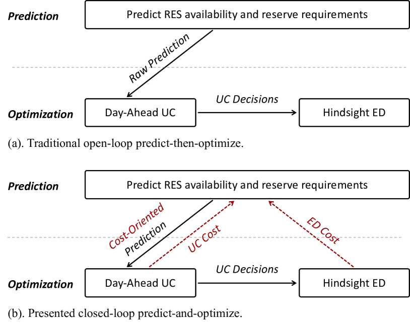
Figure 1: Comparison of traditional O-PO and proposed C-PO.          

Although the O-PO process seems practically reasonable, its operation economics suffers from two flaws: (i) The RES predictors myopically pursue statistical accuracy, such as mean absolute percentage error (MAPE), mean absolute error (MAE), and root mean square error (RMSE). However, due to the inherent nonlinearity of the UC-ED optimization process, a statistically more accurate prediction may not necessarily induce a lower system cost (as illustrated in Section III-A1); (ii) The reserve requirements sized by traditional rule-of-thumb methods may be redundant or insufficient, further worsening the economics. With this, the myopic predictions in O-PO are referred to as raw predictions in this paper.

I-B Literature Review

To improve the operation economics, one approach is to augment the deterministic UC to its two-stage stochastic programming (T-SP) [4] or two-stage robust optimization (T-RO) [5] counterpart for capturing the inaccuracy of raw predictions. Another emerging way is to form a closed loop between prediction and optimization through a feedback path, referred to as the closed-loop predict-and-optimize (C-PO). Pioneering methodologies have been explored in this direction, such as predictive prescription [6], smart predict-then-optimize (SPO) [7], and regression [8]. In a nutshell, these approaches achieve C-PO by training cost-oriented predictors to improve the performance of a specific optimization task [6, 7], or by forming prescriptive models to simultaneously realize prediction and optimization in a single step [8].

Indeed, the C-PO idea has been recently applied to several power system applications. References [9] and [10] train decision trees to predict available RES power for RES producers, which use the RES trading profit instead of entropy to evaluate prediction quality. Neural networks are trained to predict RES power for RES trading [11], load [12] and RES quantile [13] for ED, and electricity price for energy storage system arbitrage [14], in which the training loss functions explicitly quantify profit losses induced by predictions. All the references [13, 9, 10, 11, 12, 14] demonstrate that tailoring raw predictions for targeted optimization tasks can improve the economics noticeably, although the statistical prediction accuracy may be compromised to a certain extent.

Rather than grounding on heuristic methods as [13, 9, 10, 11, 12, 14], references [15, 16, 17, 18] use mathematical programming as the underlying methodology to realize C-PO. The core is to integrate predictor training and optimization tasks into an empirical risk minimization (ERM) problem, which is then solved to obtain optimal predictors. By solving the ERM problem, [15] trains an extreme learning machine to size SR requirements economically. By solving a regression-based ERM, [16] obtains a profit-oriented prescriptive model that can map feature data to RES trading decisions. The same authors further use a similar idea to formulate a value-oriented prescriptive ED in [17]. Different from [15, 16, 17] which focus on linear programming (LP) tasks, our previous work [18] customizes the SPO approach [7] for the mixed-integer programming (MIP)-based UC.

Although the methods in [15, 16, 17, 18] are regarded as stable and interpretable, their single-level ERM structures require predictor training and optimization sharing the same objective function. This restriction prevents the optimization model from meeting the practical decision-making needs of system operators, who aim to minimize the system cost instead of the training loss.

In fact, this issue can be resolved by constructing a bilevel programming-based ERM—modeling the predictor training at the upper level while uncompromisingly formulating the optimization tasks at the lower level. Following this spirit, [19] and [20] enhance their single-level ERMs in [15] and [16] to bilevel LP. Similarly, [21, 22, 23] utilize bilevel LP to construct ERM and train cost-oriented SR predictors for ED. Nevertheless, existing bilevel ERM studies are limited to LP-based ED problems.

I-C The Proposed Bilevel MIP-Based C-PO Framework

TABLE I: Review of C-PO Applications in Power Systems

Methodology Property	ERM Construction	Reference	Methodology Foundation	Prediction Term &	Optimization Task
Heuristic	-	[9]	Regression tree	RES power &	RES trading
		[10]	Classification tree [6]	RES power &	RES trading
		[11]	Extreme learning machine	RES power &	RES trading
		[12]	Deep neural network	Load &	ED
		[13]	Contextual bandit	RES power &	ED
		[14]	Deep neural network	Energy price &	Storage arbitrage
Mathematical programming	Single-level LP	[15]	Extreme learning machine	RES power and SR &	Reserve sizing
		[16]	Linear regression [8]	RES power &	RES trading
		[17]	Linear regression	Load &	ED
	Single-level MIP	[18]	Linear regression [7]	RES power &	UC
	Bilevel LP	[19]	Extreme learning machine	RES power &	ED
		[20]	Linear regression	RES power &	RES trading
		[21]	Linear regression	Load and SR &	ED
		[22]	Linear regression	SR &	ED
		[23]	Linear regression	SR and transmission ability &	ED
	Bilevel MIP	This paper	Linear regression	RES power, SR, and NR &	UC

Table I compares the proposed work with existing C-PO studies [13, 9, 10, 11, 12, 14, 15, 16, 17, 18, 19, 20, 21, 22, 23]. It is noteworthy that most mathematical programming-based studies focus on LP tasks. Differently, this paper presents a bilevel MIP-based C-PO framework, as shown in Fig. 1(b), to accurately capture system operators’ practice and deliver realizable economic improvements. Specifically, the ERM problem is constructed in the bilevel-MIP form: the upper level trains the predictors for RES power as well as SR and NR requirements; the lower level, with given upper-level predictions, includes two MIP subproblems to mimic the sequential UC-ED operation process and calculates the best possible system operation cost, which is fed back to the upper level for improving prediction quality. The ERM is converted into a bilevel MIP with only one lower-level subproblem, which is then solved by a cutting plane method [24] to deliver the optimally trained predictors of RES, SR, and NR. Finally, the predictors are integrated into the deterministic UC, forming a prescriptive UC model that delivers cost-oriented RES-SR-NR predictions and UC decisions simultaneously.

Motivated by the underlying idea of [18, 19, 20, 21, 22, 23], the proposed C-PO framework presents pioneers with MIP-based operation tasks and a tractable solution approach to accurately model operation practice for delivering realizable economic improvements. Specifically, the proposed work presents the following major distinctions:

• Bilevel-MIP Based ERM Model and Solution: References [19, 20, 21, 22, 23] exclusively focus on LP tasks that render bilevel-LP ERM problems, which can take advantage of efficient bilevel LP solution methods by substituting the lower-level LP with its Karush–Kuhn–Tucker (KKT) conditions. In comparison, in recognizing that many practical operation tasks are MIP problems, this paper presents a valuable extension of the bilevel MIP-based C-PO framework with one upper-level LP problem and two lower-level MIP subproblems, and explores its efficient solution approach. Specifically, we convert the ERM into a more tractable bilevel MIP with only one lower-level MIP subproblem, and customize the cutting plane method [24] to efficiently solve the ERM. To improve the transparency and reproducibility of the C-PO framework, all testing data and source codes are publicly accessible [25].

• Versatility, Generalization Ability, and Compatibility of Trained Predictors: Compared to our previous work [18], this paper presents three non-trivial improvements: (i) The SPO method [7] cannot predict multiple terms simultaneously. Thus, [18] can only predict RES availability or reserve requirements. In comparison, the bilevel structure enables predicting RES and multiple reserve requirements simultaneously, i.e., the presented C-PO is more versatile; (ii) Due to the single-level construction, ERM of [18] can only model the UC process with certain compromises. As a result, it can only integrate UC costs in the closed loop and remains myopic to the ED process; moreover, the feedback UC information cannot represent operators’ real decisions (Section III-A2 will explain the reasons after introducing necessary preliminaries), which is adverse to the generalization ability of predictors. In comparison, the presented bilevel ERM can feed back both UC and ED costs, forming a tighter closed loop. More importantly, the bilevel ERM enables the optimization tasks to be modeled uncompromisingly, effectively guaranteeing the generalization of predictors; (iii) Different from [18] which focuses on the comparison with O-PO, this paper additionally compares C-PO with T-SP/T-RO from an operator perspective with real-world data from a Belgian system [26]. The comparisons reveal the compatibility of the C-PO framework with the current practice and its great potential to bridge the gap between T-SP/T-RO and the practice.

The rest of the paper is organized as follows: Section II details the necessary preliminaries; Section III expounds on the C-PO framework; Section IV analyzes the experimental results; and Section V concludes this paper.

II Preliminaries

II-A Operation Models

Taking the predictions $\hat{\boldsymbol{w}}$ and $\hat{\boldsymbol{r}}$ as inputs, the operators solve the MIP-based UC model to determine the day-ahead operation plans. The compact form of UC is shown as in (1), and its detailed formulation is presented in Appendix -A. Here, $\boldsymbol{F}(\cdot)$ and $\boldsymbol{G}(\cdot)$ respectively represent the sets of equality and inequality UC constraints, forming the feasible region $\mathcal{X}$. With the predictions $\hat{\boldsymbol{w}}$ and $\hat{\boldsymbol{r}}$ as inputs, UC is solved to deliver the optimal solutions of startup, commitment, base-point generation, SR and NR schedule, as well as anticipated system cost $c^{ant\star}$ in the day-ahead stage.

$$c^{ant\star}=\textstyle{\min_{\boldsymbol{x},\boldsymbol{y}}\boldsymbol{b}^{\top}\boldsymbol{x}+\boldsymbol{c}^{\top}\boldsymbol{y}}$$ (1a)

$$\textstyle{s.\,t.\,\boldsymbol{x},\boldsymbol{y}\in\mathcal{X}(\hat{\boldsymbol{w}},\hat{\boldsymbol{r}})=\left\{\boldsymbol{x},\boldsymbol{y}\,\,\begin{array}[]{|l}\boldsymbol{F}(\boldsymbol{x},\boldsymbol{y})=0;\\ \boldsymbol{G}(\boldsymbol{x},\boldsymbol{y},\hat{\boldsymbol{w}},\hat{\boldsymbol{r}})\leq 0\end{array}\right\}}$$ (1d)

Next, with respect to the operation plans $\{\boldsymbol{x}^{\star},\boldsymbol{y}^{\star}\}$ from UC, the best possible system operations against actual RES realization $\tilde{\boldsymbol{w}}$ can be revealed by solving the MIP-based hindsight ED model. The compact form of the hindsight ED is shown as in (2), and its detailed formulation is presented in Appendix -B. Here, $\boldsymbol{M}(\cdot)$ and $\boldsymbol{N}(\cdot)$ respectively represent the sets of equality and inequality ED constraints, and $\mathcal{Z}$ is the feasible region. Solving ED provides optimal solutions to status switch of quick-start units, generation of all units, and slack variables against the RES realization $\tilde{\boldsymbol{w}}$.

$$\textstyle{\min_{\boldsymbol{z}}\boldsymbol{d}^{\top}\boldsymbol{z}}$$ (2a)

$$\textstyle{s.\,t.\,\boldsymbol{z}\in\mathcal{Z}(\boldsymbol{x}^{\star},\boldsymbol{y}^{\star},\tilde{\boldsymbol{w}})=\left\{\boldsymbol{y}\,\,\begin{array}[]{|l}\boldsymbol{M}(\boldsymbol{x}^{\star},\boldsymbol{z})=0;\\ \boldsymbol{N}(\boldsymbol{x}^{\star},\boldsymbol{y}^{\star},\boldsymbol{z},\tilde{\boldsymbol{w}})\leq 0\end{array}\mspace{-7.0mu}\right\}}\mspace{-23.0mu}$$ (2d)

The operation economics is evaluated after sequentially solving the day-ahead UC and the hindsight ED. Specifically, since $\tilde{\boldsymbol{w}}$ remains unknown in the day-ahead stage, operators first conduct UC based on $\hat{\boldsymbol{w}}$ and $\hat{\boldsymbol{r}}$, obtaining the actual UC cost (i.e., startup and no-load costs $\boldsymbol{b}^{\top}\boldsymbol{x}^{\star}$). After $\tilde{\boldsymbol{w}}$ is revealed, hindsight ED is executed based on the UC decisions, providing the hindsight ED cost $\boldsymbol{d}^{\top}\boldsymbol{z}^{\star}$ (i.e., startup and no-load costs of quick-start units additionally committed in ED, generation costs of all units, and slack penalties). With this, equation (II-A) represents the best possible system cost one can achieve in reality with respect to the UC solution and actual RES realization. This is referred to as the operation economics in this paper.

$$c^{act}= \textstyle{\sum\limits_{t\in\mathcal{T},i\in\mathcal{I}}}(C^{su}_{i}U_{it}^{\star}+C^{nl}_{i}I_{it}^{\star}) \mspace{-82.0mu}\textbf{\}}\,\boldsymbol{b}^{\top}\boldsymbol{x}^{\star}$$

$$\left.\begin{array}[]{l}\mspace{-28.0mu}+\textstyle{\sum\limits_{t\in\mathcal{T},i\in\mathcal{I}}}(C_{i}^{su}U_{it}^{ed\star}+C_{i}^{nl}I_{it}^{ed\star}+\sum\limits_{k\in\mathcal{K}}C_{ik}^{sg}P_{itk}^{ed,sg\star})\\ \mspace{-28.0mu}+\textstyle{\sum\limits_{t\in\mathcal{T}}[C^{1}S_{t}^{1\star}+C^{2}S_{t}^{2\star}+C^{bs}\sum\limits_{{b}\in\mathcal{B}}(S_{bt}^{3\star}+S_{bt}^{4\star})]}\end{array}\mspace{-10.0mu}\right\}\boldsymbol{d}^{\top}\boldsymbol{z}^{\star}$$ (5)

$$= \,\,\textstyle{\boldsymbol{b}^{\top}\boldsymbol{x}^{\star}+\boldsymbol{d}^{\top}\boldsymbol{z}^{\star}}$$ (6)

III Bilevel MIP-Based C-PO Framework

This section first illustrates the necessity of the bilevel MIP-based C-PO framework to train the cost-oriented predictors, followed by its formulation and solution method. Finally, the cost-oriented predictors obtained from the bilevel MIP-based ERM are integrated into UC to form a prescriptive UC model that can derive operation plans with improved operation economics.

III-A Why Bilevel Closed-Loop Predict-and-Optimize?

III-A1 The Asymmetric Impacts of RES Prediction Errors on Operation Economics Necessitate the C-PO

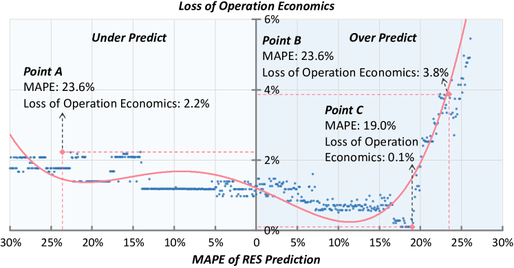
Figure 2: Asymmetric impact of RES prediction MAPE on operation economics.   

To show the asymmetry, multiple raw predictions $\hat{\boldsymbol{w}}$ on December 17, 2020 are generated based on the actual Belgian system data. These raw predictions are applied on an IEEE 14-bus system to simulate the O-PO process as shown in Fig. 1(a). Finally, the loss of operation economics is evaluated by (7), where $\hat{c}^{act}$ and $\tilde{c}^{act}$ are actual systems costs according to (II-A) with $(\hat{\boldsymbol{w}},\hat{\boldsymbol{r}})$ and $(\tilde{\boldsymbol{w}},\hat{\boldsymbol{r}})$ as inputs to UC.

$$\text{Loss of Operation Economics}=({\hat{c}^{act}-\tilde{c}^{act}})/{\tilde{c}^{act}}\times 100\%$$ (7)

Fig. 2 shows the induced results of all raw prediction points, and the red line fits the relationship between MAPE and loss of operation economics. This line clearly illustrates the asymmetry from a macro perspective. The loss caused by the over-predictions is fairly small in small-MAPE cases (MAPE of 5% to 15%), but becomes significant in large-MAPE cases (MAPE of 25% to 30%); in comparison, the loss induced by the under-predictions is relatively stable. Furthermore, two specific cases are also noteworthy:

Case 1: Raw predictions of the same MAPE may lead to different losses of operation economics. Note that points A and B in Fig. 2 have the same MAPE (23.6%) but different losses (2.2% vs 3.8%). This is because the under-prediction of point A merely causes downward generation adjustment and RES curtailments in the ED; in comparison, the over-prediction of point B requires more expensive NR deployment from quick-start units in the ED.

Case 2: Raw predictions of a worse MAPE may even lead to a smaller loss of operation economics. Although MAPE of point C is noticeably high (19.0%), it achieves the lowest loss (0.1%) among all raw predictions. This is because each $\hat{\boldsymbol{w}}$ shall be associated with a just-enough reserve level $\hat{\boldsymbol{r}}^{\star}$ with respect to $\tilde{\boldsymbol{w}}$ (i.e., a proper $\hat{\boldsymbol{r}}^{\star}$ depends on the difference between $\hat{\boldsymbol{w}}$ and $\tilde{\boldsymbol{w}}$). Consequently, if $(\hat{\boldsymbol{w}},\hat{\boldsymbol{r}}^{\star})$ is taken as input to (1), the induced UC decisions can deploy just enough reserve to enable the full utilization of available RES in actual operation, achieving the best operation economics.

As a result, the asymmetric impacts inspire that it is more proper to train the predictors based on the ultimate economic consequence of the sequential UC-ED optimization process.

III-A2 Compromised UC Modeling in the Single-Level ERM Necessitates the Bilevel MIP ERM

In the single-level ERM (8) of [18], the UC objective has to be packed into the objective function of the predictor training model as in (8a), in which $\tilde{c}^{ant}_{s}$ is the anticipated system cost (1a) induced by $(\tilde{\boldsymbol{w}}_{s},\hat{\boldsymbol{r}}_{s})$. Indeed, since (8) minimizes the in-sample training loss (8a) instead of system cost (1a), its in-sample UC solutions $\boldsymbol{x}_{s}$ may violate the least-cost merit-order principle of the system operators (i.e., using more expensive units to pursue the minimum loss function (8a)), leading to compromised UC decisions.

$$\textstyle{\min_{\mathcal{W},\boldsymbol{x}_{s},\boldsymbol{y}_{s}}} \mspace{-20.0mu}\textstyle{\frac{1}{|\mathcal{S}|}\sum_{s\in\mathcal{S}}}||\boldsymbol{b}^{\top}\boldsymbol{x}_{s}+\boldsymbol{c}^{\top}\boldsymbol{y}_{s}-\tilde{c}^{ant}_{s}||_{1}$$ (8a)

$$s.\,t. \mspace{-45.0mu}\mathcal{W}(\cdot)\in\mathcal{P}^{w};\,\,\boldsymbol{x}_{s},\boldsymbol{y}_{s}\in\mathcal{X}(\mathcal{W}(\boldsymbol{f}_{s}^{w}),\hat{\boldsymbol{r}}_{s});\,\,\,\forall s\in\mathcal{S}$$ (8b)

We draw on [20] to explain this. Indeed, given a feature $\boldsymbol{f}_{s}^{w}$, (8) cannot guarantee the induced in-sample UC decision $\{\boldsymbol{x}_{s}^{\star},\boldsymbol{y}_{s}^{\star}\}$ being the optimal solution to (1), because of the difference in objective functions (1a) and (8a). Nevertheless, as the operators are responsible for delivering the least-cost operation plans as implicated in (1a), $\{\boldsymbol{x}_{s}^{\star},\boldsymbol{y}_{s}^{\star}\}$ does not reflect the true decisions of operators. As a result, the predictor $\mathcal{W}^{\star}$ trained via these compromised UC solutions would fail to generalize well, although presenting good in-sample losses, i.e., overfitting.

In comparison, constructing ERM as a bilevel MIP can uncompromisingly integrate the exact UC model in the lower level. In this way, the in-sample UC solutions always minimize the system cost (1a), strictly following the least-cost principle. With this, using accurate feedback information can effectively avoid the overfitting issue, especially when the number of training scenarios is limited.

III-B Constructing ERM Problem

Based on the prespecified scenario set $\mathcal{S}$ (the scenario selection will be detailed in Section IV) as well as features $\boldsymbol{f}^{w}_{s}$ and $\boldsymbol{f}^{r}_{s}$, the bilevel ERM problem is constructed as in (9). The upper level (9a)-(9c) trains the predictors $\mathcal{W}$ and $\mathcal{R}$ for RES, SR, and NR , taking actual system costs as the loss function. Thus, the ERM is to maximize the weighted sum of operation economics for all scenarios. Constraint (9b) limits the predictor parameters within their feasible regions $\mathcal{P}^{w}$ and $\mathcal{P}^{r}$, and (9c) defines $\mathcal{W}$ and $\mathcal{R}$ which respectively take features $\boldsymbol{f}^{w}_{s}$ and $\boldsymbol{f}^{r}_{s}$ as inputs. The two lower-level subproblems (9d) and (9e) respectively model UC (1) and ED (2) following their original formulations exactly. Solving (9) can provide cost-oriented predictors $\mathcal{W}^{\star}$ and $\mathcal{R}^{\star}$.

Upper Level (Predictor Training):

$$\textstyle{\min_{\mathcal{W},\mathcal{R}}}\textstyle{\frac{1}{|\mathcal{S}|}\sum_{s\in\mathcal{S}}}\boldsymbol{b}^{\top}\boldsymbol{x}_{s}+\boldsymbol{d}^{\top}\boldsymbol{z}_{s}$$ (9a)

$$\mathcal{W}(\cdot)\in\mathcal{P}^{w};\,\,\mathcal{R}(\cdot)\in\mathcal{P}^{r}$$ (9b)

$$\hat{\boldsymbol{w}}^{\diamond}_{s}=\mathcal{W}(\boldsymbol{f}^{w}_{s});\,\,\hat{\boldsymbol{r}}^{\diamond}_{s}=\mathcal{R}(\boldsymbol{f}^{r}_{s}); \mspace{-85.0mu}\forall s\in\mathcal{S}$$ (9c)

Lower Level (Day-Ahead UC):

$$\boldsymbol{x}_{s},\boldsymbol{y}_{s}\in{\arg\min}_{\boldsymbol{x}_{s},\boldsymbol{y}_{s}\in\mathcal{X}(\hat{\boldsymbol{w}}^{\diamond}_{s},\hat{\boldsymbol{r}}^{\diamond}_{s})}\boldsymbol{b}^{\top}\boldsymbol{x}_{s}+\boldsymbol{c}^{\top}\boldsymbol{y}_{s}; \mspace{-85.0mu}\forall s\in\mathcal{S}$$ (9d)

Lower Level (Hindsight ED):

$$\boldsymbol{z}_{s}\in{\arg\min}_{\boldsymbol{z}_{s}\in\mathcal{Z}(\boldsymbol{x}_{s},\boldsymbol{y}_{s},\tilde{\boldsymbol{w}}_{s})}\boldsymbol{d}^{\top}\boldsymbol{z}_{s}; \mspace{-85.0mu}\forall s\in\mathcal{S}$$ (9e)

In this paper, affine linear functions are used to form the predictors, as shown in (10), because of their interpretability [16] and numerical stability [17]. The symbol $\circ$ indicates the element-wise product. As for features, the raw prediction $\hat{\boldsymbol{w}}$ is used for $\boldsymbol{f}^{w}_{s}$ as in (10a), which is suggested by a standard coefficient regression method [27]. In this way, the C-PO is an upgraded version based on the O-PO, i.e., the operators can continue using the original predictors and improve them. In addition, the load prediction $\hat{\boldsymbol{l}}$ and RES prediction $\hat{\boldsymbol{w}}$ are used to form $\boldsymbol{f}^{r}$, as in (10b). This is because (i) Common feature selection methods (e.g., standard coefficient regression and principal component analysis) are not applicable to our case, as they need the just-enough reserve level $\hat{\boldsymbol{r}}^{\star}$ as input labels which however cannot be obtained until $\hat{\boldsymbol{w}}$ is revealed; and (ii) It is well recognized that reserve requirements are mainly driven by load and RES uncertainties. With this, the feasible regions $\mathcal{P}^{w}$ and $\mathcal{P}^{r}$ are set as the positive real-number region $\mathbb{R}_{+}$ of appropriate dimensions. The training is basically to determine the optimal vectors $\boldsymbol{m}$ and $\boldsymbol{n}$.

$$\mspace{-3.0mu}\mathcal{W}(\boldsymbol{f}^{w}_{s})=\boldsymbol{m}\circ\boldsymbol{f}^{w}_{s}\Rightarrow\mathcal{W}(\hat{\boldsymbol{w}}_{s})=\boldsymbol{m}\circ\hat{\boldsymbol{w}}_{s};\boldsymbol{m}\in\mathbb{R}_{+}^{|\mathcal{T}|\times|\mathcal{J}|}$$ (10a)

$$\mspace{-3.0mu}\mathcal{R}(\boldsymbol{f}^{r}_{s})=\boldsymbol{n}\circ\boldsymbol{f}^{r}_{s}\Rightarrow\mathcal{R}(\hat{\boldsymbol{w}}_{s},\hat{\boldsymbol{l}}_{s})=\boldsymbol{n}\circ(\hat{\boldsymbol{w}}_{s},\hat{\boldsymbol{l}}_{s});\boldsymbol{n}\in\mathbb{R}_{+}^{|\mathcal{T}|\times 2}$$ (10b)

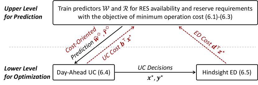
Figure 3: Illustration of the closed-loop mechanism in bilevel ERM.        

As a specific form of Fig. 1(b), Fig. 3 depicts how the bilevel ERM (9) enables the interaction between the predictions and optimizations to form the closed loop. The upper level generates the tailored predictions $\hat{\boldsymbol{w}}^{\diamond}$ and $\hat{\boldsymbol{r}}^{\diamond}$, but cannot directly assess their ultimate economic consequence. Thus, $\hat{\boldsymbol{w}}^{\diamond}$ and $\hat{\boldsymbol{r}}^{\diamond}$ are first passed to the lower-level day-ahead UC (9d), forming the UC feasible region $\mathcal{X}$. Solving (9d) provides the actual UC cost $\boldsymbol{b}^{\top}\boldsymbol{x}^{\star}$ to the upper level as well as the UC decisions $\{\boldsymbol{x}^{\star},\boldsymbol{y}^{\star}\}$ to the lower-level hindsight ED (9e). Taking the UC decisions as inputs, (9e) is solved to further provide the hindsight ED cost $\boldsymbol{d}^{\top}\boldsymbol{z}^{\star}$ to the upper level. With this, the upper level can assess the prediction quality via actual system cost $\boldsymbol{b}^{\top}\boldsymbol{x}^{\star}+\boldsymbol{d}^{\top}\boldsymbol{z}^{\star}$, and tune the predictor parameters accordingly. This process repeats until the optimally trained predictors $\mathcal{W}^{\star}$ and $\mathcal{R}^{\star}$ (i.e., vectors $\boldsymbol{m}$ and $\boldsymbol{n}$ in (10)) are obtained. Since $\mathcal{W}^{\star}$ and $\mathcal{R}^{\star}$ are trained to optimize the operation cost, they are cost-oriented and tailored for system operations.

III-C Solving ERM Problem

III-C1 Convert (6) with Two MIP Subproblems in the Lower Level to (8) with One MIP in the Lower Level

The bilevel ERM (9) includes two MIP subproblems in the lower level, introducing extra computational complexity. With this, we first convert (9) into a more tractable bilevel MIP (11) with one MIP in the lower level. Solving (11) provides the optimal solution of the original ERM (9), as stated in Proposition 1.

Proposition 1

The optimal solution of the bilevel MIP (11) is also optimal to the original bilevel MIP (9).

$$\textstyle{\min_{\mathcal{W},\mathcal{R},\boldsymbol{z}_{s}}} \mspace{-70.0mu}\textstyle{\frac{1}{|\mathcal{S}|}\sum_{s\in\mathcal{S}}}\boldsymbol{b}^{\top}\boldsymbol{x}_{s}+\boldsymbol{d}^{\top}\boldsymbol{z}_{s}$$ (11a)

$$\,\,s.\,t. \mspace{-70.0mu}\mathcal{W}(\cdot)\in\mathcal{P}^{w};\,\,\mathcal{R}(\cdot)\in\mathcal{P}^{r}$$ (11b)

$$\mspace{-70.0mu}\hat{\boldsymbol{w}}^{\diamond}_{s}=\mathcal{W}(\boldsymbol{f}^{w}_{s});\,\,\hat{\boldsymbol{r}}^{\diamond}_{s}=\mathcal{R}(\boldsymbol{f}^{r}_{s}); \mspace{-50.0mu}\forall s\in\mathcal{S}$$ (11c)

$$\mspace{-70.0mu}\boldsymbol{z}_{s}\in\mathcal{Z}(\boldsymbol{x}_{s},\boldsymbol{y}_{s},\tilde{\boldsymbol{w}}_{s}); \mspace{-50.0mu}\forall s\in\mathcal{S}$$ (11d)

$$\mspace{-70.0mu}\boldsymbol{x}_{s},\boldsymbol{y}_{s}\in\underset{\boldsymbol{x}_{s},\boldsymbol{y}_{s}\in\mathcal{X}(\hat{\boldsymbol{w}}^{\diamond}_{s},\hat{\boldsymbol{r}}^{\diamond}_{s})}{\arg\min}\boldsymbol{b}^{\top}\boldsymbol{x}_{s}+\boldsymbol{c}^{\top}\boldsymbol{y}_{s}; \mspace{-50.0mu}\forall s\in\mathcal{S}$$ (11e)

Proof:

See Appendix -C. ∎

III-C2 Solve (8) by C&CG Algorithm

The bilevel MIP (11) is solved via a column-and-constraint generation (C&CG) algorithm [24], which iterates between the master problem MP and two subproblems SP1 and SP2. The process is summarized in Algorithm 1.

The first subproblem SP1 is shown as in (12). It is a duplication of the UC problem (11e) while taking the incumbent predictors $\mathcal{W}_{e}$ and $\mathcal{R}_{e}$ as inputs. Solving SP1 can reveal the anticipated system cost $c_{s}^{ant\star}$ induced by the incumbent predictors.

SP1: $$c^{ant\star}_{s}= \mspace{-20.0mu}\textstyle{\min_{\boldsymbol{x}_{s},\boldsymbol{y}_{s}}\boldsymbol{b}^{\top}\boldsymbol{x}_{s}+\boldsymbol{c}^{\top}\boldsymbol{y}_{s}}$$ (12a)

$$s.\,t.\, \mspace{-20.0mu}\hat{\boldsymbol{w}}^{\diamond}_{s}=\mathcal{W}_{e}(\boldsymbol{f}^{w}_{s});\,\,\hat{\boldsymbol{r}}^{\diamond}_{s}=\mathcal{R}_{e}(\boldsymbol{f}^{r}_{s})$$ (12b)

$$\mspace{-20.0mu}\boldsymbol{F}(\boldsymbol{x}_{s},\boldsymbol{y}_{s})=0;\,\,\boldsymbol{G}(\boldsymbol{x}_{s},\boldsymbol{y}_{s},\hat{\boldsymbol{w}}^{\diamond}_{s},\hat{\boldsymbol{r}}^{\diamond}_{s})\leq 0$$ (12c)

Note that multiple optimal binaries $\boldsymbol{x}_{s}^{\star}$ for SP1 may exist, which however could lead to different system costs evaluated via (11a). Thus, the second subproblem SP2, formed as in (13) with $c^{ant\star}_{s}$ from SP1 as input, is further solved to select a solution among multiple optimal binaries $\boldsymbol{x}_{s}^{\star}$ of SP1 in favor of the objective (11a). This is referred to as optimistic bilevel programming [24].

SP2: $$c_{s}^{act\star}= \mspace{-10.0mu}\textstyle{\min_{\boldsymbol{x}_{s},\boldsymbol{y}_{s},\boldsymbol{z}_{s}}\boldsymbol{b}^{\top}\boldsymbol{x}_{s}+\boldsymbol{d}^{\top}\boldsymbol{z}_{s}}$$ (13a)

$$s.\,t. \mspace{-30.0mu}\hat{\boldsymbol{w}}^{\diamond}_{s}=\mathcal{W}_{e}(\boldsymbol{f}^{w}_{s});\,\,\hat{\boldsymbol{r}}^{\diamond}_{s}=\mathcal{R}_{e}(\boldsymbol{f}^{r}_{s})$$ (13b)

$$\mspace{-30.0mu}\boldsymbol{b}^{\top}\boldsymbol{x}_{s}+\boldsymbol{c}^{\top}\boldsymbol{y}_{s}\leq c^{ant\star}_{s}$$ (13c)

$$\mspace{-30.0mu}\boldsymbol{F}(\boldsymbol{x}_{s},\boldsymbol{y}_{s})=0;\,\,\boldsymbol{G}(\boldsymbol{x}_{s},\boldsymbol{y}_{s},\hat{\boldsymbol{w}}^{\diamond}_{s},\hat{\boldsymbol{r}}^{\diamond}_{s})\leq 0$$ (13d)

$$\mspace{-30.0mu}\boldsymbol{M}(\boldsymbol{x}_{s},\boldsymbol{z}_{s})=0;\,\,\boldsymbol{N}(\boldsymbol{x}_{s},\boldsymbol{y}_{s},\boldsymbol{z}_{s},\tilde{\boldsymbol{w}}_{s})\leq 0$$ (13e)

Given the selected decisions $\boldsymbol{x}_{s}^{\star}$ from SP2, the master problem MP (14) is formulated as the high-point problem [24] of (11). Three sets of variants for variables $\{\boldsymbol{x}_{s},\boldsymbol{y}_{s}\}$ are used in MP, including duplicated variables $\{\boldsymbol{x}^{dv}_{s},\boldsymbol{y}^{dv}_{s}\}$, enumerated binary variables $\boldsymbol{x}^{ev}_{s,e}$, and generated continuous variables $\boldsymbol{y}^{gv}_{s,e}$. The duplicated variables server as the proxy of the original variables, but with a larger feasible region; the enumerated and generated variables and their associated cutting planes (14f)-(14i) serve to cut the feasible region of duplicated variables gradually. MP is built in three parts:

• The first part (14a)-(14d) is based on the duplicated variables. The objective (14a) also includes two regularization terms $+\lambda^{w}\lVert\mathcal{W}\rVert_{1}$ (avoid over-predictions) and $-\lambda^{r}\lVert\mathcal{R}\rVert_{1}$ (avoid insufficient reserves) with hyper-parameters $\lambda^{w/r}$. Note that the regularization terms could be removed when the number of scenarios is sufficient. Constraints (14b)-(14d) correspond to the original upper-level constraints (11b)-(11d).

• The second part (14e) is a duplication of UC constraints to ensure the feasibility of the duplicated variables.

• The third part (14f)-(14i) servers as the optimality cuts for the duplicated variables. Note that $\boldsymbol{x}^{ev}_{s,e}$ is a constant vector enumerated by SP2 (i.e., $\boldsymbol{x}^{ev}_{s,e}$ is fixed as the selected $\boldsymbol{x}_{s}^{\star}$) for scenario $s$ in iteration $e$. When $\boldsymbol{x}_{s}$ is fixed as $\boldsymbol{x}^{ev}_{s,e}$, (11e) degenerates to an LP and is equivalently substituted by the KKT condition (14f)-(14h). Here, $\mathcal{L}(\cdot)$ denotes the Lagrangian function; $\boldsymbol{\mu}$ and $\boldsymbol{\nu}$ are dual variables of equalities and inequalities. The KKT conditions (14f)-(14h) ensure the optimality of the generated variables given $\boldsymbol{x}^{ev}_{s,e}$. Finally, (14i) links the duplicated variables with their optimality cuts.

$$\textbf{MP:}\,\min_{\Xi}\textstyle{\frac{1}{|\mathcal{S}|}\sum_{s\in\mathcal{S}}}(\boldsymbol{b}^{\top}\boldsymbol{x}^{dv}_{s}+\boldsymbol{d}^{\top}\boldsymbol{z}_{s})+\lambda^{w}\lVert\mathcal{W}\rVert_{1}-\lambda^{r}\lVert\mathcal{R}\rVert_{1}\mspace{-19.0mu}$$

$$\Xi=\{\mathcal{W}(\cdot),\mathcal{R}(\cdot),\hat{\boldsymbol{w}}^{\diamond}_{s},\hat{\boldsymbol{r}}^{\diamond}_{s},\boldsymbol{z}_{s},\boldsymbol{x}^{dv}_{s},\boldsymbol{y}^{dv}_{s},\boldsymbol{y}^{gv}_{s}\}\mspace{-20.0mu}$$ (14a)

Original Constraints:

$$\mathcal{W}(\cdot)\in\mathcal{P}^{w};\,\,\mathcal{R}(\cdot)\in\mathcal{P}^{r}$$ (14b)

$$\hat{\boldsymbol{w}}^{\diamond}_{s}=\mathcal{W}(\boldsymbol{f}^{w}_{s});\,\,\hat{\boldsymbol{r}}^{\diamond}_{s}=\mathcal{R}(\boldsymbol{f}^{r}_{s}); \,\,\mspace{-155.0mu}\forall s\in\mathcal{S}$$ (14c)

$$\boldsymbol{M}(\boldsymbol{x}^{dv}_{s},\boldsymbol{z}_{s})=0;\,\,\boldsymbol{N}(\boldsymbol{x}^{dv}_{s},\boldsymbol{y}^{dv}_{s},\boldsymbol{z}_{s},\tilde{\boldsymbol{w}}_{s})\leq 0; \,\,\mspace{-155.0mu}\forall s\in\mathcal{S}$$ (14d)

Duplication of UC Constraints:

$$\boldsymbol{F}(\boldsymbol{x}_{s}^{dv},\boldsymbol{y}_{s}^{dv})=0;\,\,\boldsymbol{G}(\boldsymbol{x}^{dv}_{s},\boldsymbol{y}_{s}^{dv},\hat{\boldsymbol{w}}_{s}^{\diamond},\hat{\boldsymbol{r}}_{s}^{\diamond})\leq 0; \,\,\mspace{-155.0mu}\forall s\in\mathcal{S}$$ (14e)

Stationarity of KKT (Optimality Cut):

$$\nabla\mathcal{L}(\boldsymbol{y}_{s,e}^{gv},\boldsymbol{\mu}_{s,e},\boldsymbol{\nu}_{s,e})=0; \,\,\mspace{-155.0mu}\forall s\in\mathcal{S}$$ (14f)

Primal and Dual Feasibilities of KKT (Optimality Cut):

$$\boldsymbol{F}(\boldsymbol{x}_{s,e}^{ev},\boldsymbol{y}_{s,e}^{gv})=0;$$

$$\boldsymbol{G}(\boldsymbol{x}_{s,e}^{ev},\boldsymbol{y}_{s,e}^{gv},\hat{\boldsymbol{w}}_{s}^{\diamond},\hat{\boldsymbol{r}}_{s}^{\diamond})\leq 0;\,\,\boldsymbol{\nu}_{s,e}\geq 0; \,\,\mspace{-155.0mu}\forall s\in\mathcal{S},e\in\mathcal{E}$$ (14g)

Complementary Slackness of KKT (Optimality Cut):

$$\boldsymbol{\nu}_{s,e}\bot\boldsymbol{G}(\boldsymbol{x}_{s,e}^{ev},\boldsymbol{y}_{s,e}^{gv},\hat{\boldsymbol{w}}_{s}^{\diamond},\hat{\boldsymbol{r}}_{s}^{\diamond}); \,\,\mspace{-155.0mu}\forall s\in\mathcal{S},e\in\mathcal{E}$$ (14h)

Objective Cut (Optimality Cut):

$$\boldsymbol{b}^{\top}\boldsymbol{x}_{s}^{dv}+\boldsymbol{c}^{\top}\boldsymbol{y}_{s}^{dv}\leq\boldsymbol{b}^{\top}\boldsymbol{x}_{s,e}^{ev}+\boldsymbol{c}^{\top}\boldsymbol{y}_{s,e}^{gv}; \,\,\mspace{-155.0mu}\forall s\in\mathcal{S},e\in\mathcal{E}$$ (14i)

By linearizing the complementary slackness (14h) via the Big-M method [28], MP can be converted into a MIP problem and directly solved by commercial MIP solvers. The user-friendly KKT and export functions of YALMIP [29] are used to facilitate the implementation of KKT constraints (14f)-(14h).

Input: Index of iterations $e=0$ and its limitation $E$, desired optimality gap $\epsilon^{\star}$, initial predictors $\mathcal{W}_{e}$ and $\mathcal{R}_{e}$, lower bound $LB$, and upper bound $UB$.

Output: Well-trained predictors $\mathcal{W}^{\star}$ and $\mathcal{R}^{\star}$.

while $e\leq E$ do

       Solve SP1 and SP2 for each scenario $s\in\mathcal{S}$;

       $UB\leftarrow\min\{UB,\sum_{s\in\mathcal{S}}c_{s}^{act\star}/|\mathcal{S}|+\lambda^{w}\lVert\mathcal{W}\rVert_{1}-\lambda^{r}\lVert\mathcal{R}\rVert_{1}\}$;

       $\epsilon\leftarrow 100\%\times(UB-LB)/UB$;

       if $\epsilon\leq\epsilon^{\star}$ then

             $\mathcal{W}^{\star}\leftarrow\mathcal{W}_{e}$, $\mathcal{R}^{\star}\leftarrow\mathcal{R}_{e}$;

             break;

            

      else

             $\boldsymbol{x}_{s,e}^{ev}$ $\leftarrow$ optimal solution of decision $\boldsymbol{x}_{s}$ in SP2;

             Generate new $\{\boldsymbol{x}^{gv}_{s,e},\boldsymbol{y}^{gv}_{s,e}\}$ and cuts (14f)-(14i) in MP;

             Solve MP;

             $e\leftarrow e+1,LB\leftarrow$ optimal objective value of MP;

             $\mathcal{W}_{e}$ and $\mathcal{R}_{e}$ $\leftarrow$ optimal $\mathcal{W}$ and $\mathcal{R}$ from MP;

            

       end if

      

end while

Algorithm 1 A C&CG Algorithm for Solving (11)

III-D Forming Prescriptive UC Model

The prescriptive UC model (15) is formed by integrating the trained cost-oriented predictors $\mathcal{W}^{\star}$ and $\mathcal{R}^{\star}$ into the deterministic UC model (1). It possesses two major favorable properties as compared to the deterministic UC model (1):

• Integrating the predictors enables (15) to simultaneously deliver the RES-reserve predictions and UC decisions, referred to as prescription. In comparison, in the O-PO framework, (1) exclusively focuses on the UC decision, and most existing forecasting works mainly focus on the prediction.

• $\mathcal{W}^{\star}$ and $\mathcal{R}^{\star}$ are affine linear functions (10). Therefore, the tailored predictions are essentially the linear combination of the raw predictions, which will not significantly complicate the computation of (15).

$$\textstyle{\min_{\boldsymbol{x},\boldsymbol{y},\hat{\boldsymbol{w}}^{\diamond},\hat{\boldsymbol{r}}^{\diamond}}\boldsymbol{b}^{\top}\boldsymbol{x}+\boldsymbol{c}^{\top}\boldsymbol{y}}$$ (15a)

$$\,\,s.\,t.\,\boldsymbol{x},\boldsymbol{y}\in\mathcal{X}(\hat{\boldsymbol{w}}^{\diamond},\hat{\boldsymbol{r}}^{\diamond});\,\hat{\boldsymbol{w}}^{\diamond}=\mathcal{W}^{\star}(\boldsymbol{f}^{w});\,\hat{\boldsymbol{r}}^{\diamond}=\mathcal{R}^{\star}(\boldsymbol{f}^{r})$$ (15b)

Finally, the presented C-PO framework replaces the deterministic UC model (1) with the prescriptive UC model (15) to boost operation economics.

IV Case Studies

IV-A Experimental Setting

IV-A1 C-PO Implementation Design

To leverage compatibility with the system operators’ practice and solution quality of (15), the proposed C-PO is implemented via a weekly rolling scheme. That is, for each week, the predictors are retrained to update (15) using the information of the past $NT$ days.

Specifically, to study the dispatch week of days $(D+\text{1})$ to $(D+\text{7})$, the past $NT$ days (i.e., days $(D-NT)$ to $(D-\text{1}))$ are selected to build the training scenario set $\mathcal{S}$. Then, the ERM (9) is solved to provide the cost-oriented predictors $\mathcal{W}^{\star}$ and $\mathcal{R}^{\star}$, which are used to form the prescriptive UC models (15) for each of days $(D+\text{1})$ to $(D+\text{7})$. At the end of this period, the above process repeats to update the predictors and solve (15) for the next week (i.e., days $(D+\text{8})$ to $(D+\text{14})$).

IV-A2 Experimental Setup

Based on the Belgian system data [26], four weeks in 2020 as shown in Table II are selected, representing peak RES availabilities in the four quarters. The Belgian data are scaled to build the RES and load data for the test systems. The slack penalty prices $C^{1}$, $C^{2}$, and $C^{bs}$ are all set as $2,000/MWh. The rule-of-thumb reserve requirement is set according to the CAISO practice: system reserve requirement represented as a proper proportion $\alpha$ of the load is met by non-RES units, of which at least 50% is SR. Other data can be referred to from [25].

Table III lists all the models to be analyzed. The threshold on the optimality gap of all models is set as 1%. For C-PO-NTs, the hyper-parameters $\lambda^{w/r}$ are set as $\text{10}^{\text{6}}$. As the magnitude of the actual system cost $c^{act}$ (11a) is between $\text{10}^{\text{5}}$ and $\text{10}^{\text{6}}$, a hyper-parameter of $\text{10}^{\text{6}}$ would present a sufficient, but not overly dominating, effect on the ERM problem. All cases are solved by Gurobi 9.1, called by YALMIP on MATLAB, on a 3.5 GHz PC.

TABLE II: Selective Weeks of 2020

Quarter 1	Quarter 2	Quarter 3	Quarter 4
Feb 04 – Feb 09	Jun 28 – Jul 04	Aug 20 – Aug 26	Dec 12 – Dec 18

TABLE III: Methods to Be Discussed

Acronym	Note
C-PO-NT	Presented C-PO framework with $NT$ training scenarios.
C-PO-NT-R	C-PO-NT that only predicts reserves $\hat{\boldsymbol{r}}^{\diamond}$ and keeps raw RES $\hat{\boldsymbol{w}}$.
C-PO-NT-W	C-PO-NT that only predicts RES $\hat{\boldsymbol{w}}^{\diamond}$ and keeps raw reserves $\hat{\boldsymbol{r}}$.
O-PO	Traditional O-PO framework with raw $\hat{\boldsymbol{r}}$ and $\hat{\boldsymbol{w}}$.
P-PO	Perfect predict-then-optimize that uses RES realization $\tilde{\boldsymbol{w}}$ as raw
	RES prediction $\hat{\boldsymbol{w}}$ and keeps raw reserves $\hat{\boldsymbol{r}}$.
T-SP-NS	Two-stage stochastic programming with $NS$ scenarios.
T-RO-NB	Two-stage robust optimization with budget parameter $\Gamma$ = $NB$.

IV-B C-PO vs O-PO

Based on an IEEE 14-bus system (with $\alpha$ = 50%, 1,700MW non-RES capacity, and 400MW RES capacity), this section compares C-PO and O-PO via two metrics: economics improvement (EI) (16) to evaluate improvement in operation costs and value of information (VoI) (17) to quantify the value of feedback information.

$$\mspace{-8.0mu}\text{EI}=({c^{act,o\text{-}po}-c^{act,c\text{-}po}})/({c^{act,o\text{-}po}})\times 100\%$$ (16)

$$\mspace{-8.0mu}\text{VoI}=({c^{act,o\text{-}po}-c^{act,c\text{-}po}})/({c^{act,o\text{-}po}-c^{act,p\text{-}po}})$$ (17)

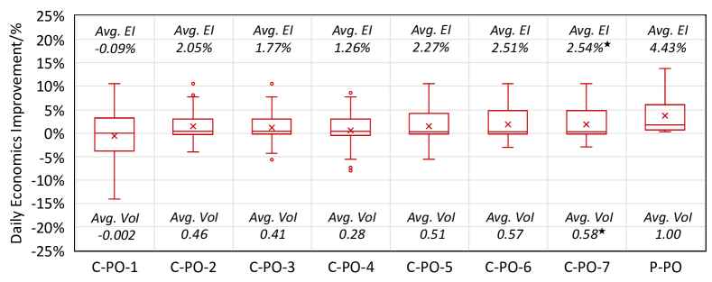
Figure 4: Economics comparison of O-PO, C-PO, and P-PO.            

TABLE IV: Breakdown of Actual System Cost

	Actual UC Cost/$\text{10}^{\text{3}}$$		Hindsight ED Cost/$\text{10}^{\text{3}}$$			$c^{act}$/$\text{10}^{\text{3}}$$
	Startup	No-Load	Startup	No-Load	Gen.
O-PO	1.1	2.1	0.1	0.1	237.9	241.3
C-PO-7	1.0	2.2	0.1	0.1	231.9	235.3

TABLE V: Comparison of Different C-PO Methods

	Scheduled Reserve		Training		EI
	SR/MW	NR/MW	CPU Time/s	# of Iterations
O-PO	113.2	113.2	-	-	0.00%
C-PO-1	110.8	75.6	19	2	-0.09%
C-PO-7	92.9	65.4	786	6	2.54%
C-PO-1-W	113.2	113.2	21	2	-0.22%
C-PO-7-W	113.2	113.2	750	3	-0.02%
C-PO-1-R	98.8	85.8	13	2	-0.48%
C-PO-7-R	88.8	63.3	1,857	4	1.77%

TABLE VI: Statistical Accuracy of RES Prediction

	MAE/MW	RMSE/MW	MAPE	MOPE	MUPE
$\hat{\boldsymbol{w}}$ in O-PO	15.0	21.0	36.4%	29.6%	6.8%
$\hat{\boldsymbol{w}}^{\diamond}$ in C-PO-7	16.5	23.2	35.9%	27.7%	8.2%

IV-B1 Results

Fig. 4 shows that all the six C-PO-NT models with $NT$ = 2 to 7 outperform O-PO economically, in which C-PO-7 renders the best performance (i.e., 2.54% average EI and 0.58 average VoI). As the ideal P-PO with the 1.00 VoI only achieves 4.43% EI, the 2.54% EI of C-PO-7 could be regarded as non-trivial.

Table IV breakdowns the actual system costs of O-PO and C-PO-7. The main difference between O-PO and C-PO-7 stems from the generation cost in ED. It is also noteworthy that C-PO-7 has a lower startup cost and a higher no-load cost in UC.

Table V compares different C-POs. It shows that C-PO-NTs and C-PO-NT-Rs render lower SR and NR than the raw schedules, among which SR is always higher than NR. Regarding the training, both computational time and the number of iterations for solving the ERM problem increase with $NT$. Moreover, it is noteworthy that four C-POs cause negative EI.

Finally, Table VI evaluates RES prediction accuracy via five metrics, including MAE, RMSE, MAPE, mean over-prediction percentage error (MOPE), and mean under-prediction percentage error (MUPE). Compared to O-PO, C-PO-7 has a better MAPE but worse MAE and RMSE. Moreover, C-PO-7 has a better MOPE but a worse MUPE, indicating that C-PO-7 tends to conservatively predict RES power (i.e., $\hat{\boldsymbol{w}}^{\diamond}$ is statistically smaller than $\hat{\boldsymbol{w}}$).

IV-B2 Discussions

The results clearly show that C-PO outperforms O-PO in terms of operation economics. Still, the reasons behind this conclusion and potential issues deserve further discussion.

Table IV shows that the economic difference mainly stems from the generation. This is because C-PO-7 takes advantage of the units with cheaper generation costs. Although these units have higher no-load costs, C-PO-7 keeps them online longer enough by setting the predictions $\hat{\boldsymbol{w}}^{\diamond}$ and $\hat{\boldsymbol{r}}^{\diamond}$ properly. As a result, C-PO-7 uses fewer units in ED, and operates them in the most efficient condition.

According to Table V, C-POs believe a proper reserve deployment should have a higher SR and a lower NR, instead of half-and-half. This is because the bilevel ERM enables C-POs to learn that triggering quick-start units in ED is more expensive. Moreover, although reserve requirements of C-POs are lower than those of O-PO in general, our experiments show that (i) Reserve requirements of C-PO-7 are 5.28% higher than those of O-PO in quarter 2, indicating that the rule-of-thumb $\hat{\boldsymbol{r}}$ may be insufficient in certain cases; and (ii) C-PO-NTs leverage lower $\hat{\boldsymbol{w}}^{\diamond}$ and higher base-generation $P_{it}^{\star}$ in the day-ahead UC, allowing system operators to possess enough capacity and avoid load shedding when faced with $\tilde{\boldsymbol{w}}$ in actual operations. As a result, it can be pointed out that C-POs tailor the predictions for the operation problem suitably. Last but not least, two more points can be implied by Table V:

• Negative EIs indicate that closed-loop learning may lead to an adverse impact on operation economics. Indeed, C-PO possesses the common issue in wide machine learning methods—it cannot fully guarantee that learning will always bring in extra benefits. Nevertheless, this issue could be relieved with sufficient training scenarios and well-tuned hyper-parameters.

• Although EI monotonically increases with $NT$ in Table V when multiple scenarios are used for training, Fig. 4 indicates that this relationship may not hold in a 1-scenario grain. Two possible reasons are responsible for this fluctuation: (i) A single predictor is used throughout one week, regardless of weekdays and weekends; and (ii) The number of training scenarios is limited. To relieve the fluctuation, the first approach is to train different predictors for weekdays and weekends, and the second approach is to increase $NT$—the best performance is generally achieved when $NT$ reaches about 10 times the number of predictor parameters. However, these two approaches would significantly increase the training cost. Therefore, system operators should weigh up the pros and cons according to the computational budget.

As shown in Table VI, C-PO-7 performs worse in MAE and RMSE. This is because C-PO evaluates the prediction quality by actual operation cost $c^{act}$ instead of traditional statistical metrics. Nevertheless, it is interesting to observe that C-PO-7 outperforms O-PO in MAPE. This is because C-PO-7 generally under-predicts RES, hence the MAPE of $\hat{\boldsymbol{w}}^{\diamond}$ is smaller than that of $\hat{\boldsymbol{w}}$ in the cases of scarce RES. However, these cases have a limited impact on both MAE and RMSE, because they are relatively insensitive to small values. Accordingly, Table VI implies a fact—judging prediction quality with a single statistical metric could be one-sided, as each metric owns a specific property. To this end, this paper suggests evaluating the prediction quality with the ultimate operation goal.

In summary, by effectively leveraging the bilevel MIP structure to learn the UC-ED optimization information, C-PO tailors raw ($\hat{\boldsymbol{w}},\hat{\boldsymbol{r}}$) to cost-oriented ($\hat{\boldsymbol{w}}^{\diamond},\hat{\boldsymbol{r}}^{\diamond}$) for improving operation economics. Even though the tailored predictions are slightly worse in certain statistical metrics, they enable the system to operate more economically. As a result, C-PO significantly outperforms O-PO in terms of operation cost. Nevertheless, the reduction in prediction accuracy, as shown in Table VI, shall not be considered a compromise, because the ultimate goal of the prediction is to improve the optimization performance instead of simply improving the prediction accuracy. Moreover, the presented C-PO framework is built on top of the system operators’ accuracy-oriented predictors and thus is compatible with their current practice.

IV-C C-PO vs Two-Stage Optimization Models with MIP Recourse

Based on a modified IEEE 118-bus system (with 8,600MW non-RES capacity and 1,000MW RES capacity), C-PO, T-SP, and T-RO are compared on the first day for each of the four weeks listed in Table II. For the sake of comparison, the following settings on the T-SP and T-RO models with MIP recourse are adopted:

• Load and RES are regarded as uncertainty factors, whose prediction and actual realization are denoted as $\hat{\boldsymbol{u}}$ and $\tilde{\boldsymbol{u}}$, respectively. The day-ahead point forecast and the 90% confidence interval for $\hat{\boldsymbol{u}}$ are built based on [26].

• T-SP is modeled as a scenario-based model [4] via (18). To construct the scenario set $\mathcal{H}$, 3,000 scenarios are generated via Latin hypercube sampling within the 90% confidence interval, and then reduced to $NS$ scenarios via a scenario-tree method [30]. $p_{h}$ denotes the probability of scenario $h$. (18) is solved by Gurobi 9.1 directly.

  $$\textstyle{\min_{\boldsymbol{x},\boldsymbol{y},\boldsymbol{z}}} \,\,\boldsymbol{b}^{\top}\boldsymbol{x}+\boldsymbol{c}^{\top}\boldsymbol{y}+p_{h}\textstyle{\sum_{h\in\mathcal{H}}\boldsymbol{d}^{\top}\boldsymbol{z}_{h}}$$ (18a)

  $$s.\,t.\, \,\,\boldsymbol{x},\boldsymbol{y}\in\mathcal{X}(\hat{\boldsymbol{u}});\,\,\boldsymbol{z}_{h}\in\mathcal{Z}(\boldsymbol{x},\boldsymbol{y},\tilde{\boldsymbol{u}}_{h});\,\,\forall h\in\mathcal{H}$$ (18b)

• T-RO is modeled as an adjustable RO [5] via (19). The box uncertainty set $\mathcal{U}$ is constructed using the 90% confidence intervals, and the budget parameter $\Gamma\in[\text{0},\text{48}]$ controls the robustness. We use a nested C&CG method [31] to solve (19).

  $$\textstyle{\min_{\boldsymbol{x},\boldsymbol{y}}} \,\,\boldsymbol{b}^{\top}\boldsymbol{x}+\boldsymbol{c}^{\top}\boldsymbol{y}+\textstyle{\max_{\tilde{\boldsymbol{u}}\in\mathcal{U}}\min_{\boldsymbol{z}}}\boldsymbol{d}^{\top}\boldsymbol{z}$$ (19a)

  $$s.\,t. \,\,\boldsymbol{x},\boldsymbol{y}\in\mathcal{X}(\hat{\boldsymbol{u}});\,\,\boldsymbol{z}\in\mathcal{Z}(\boldsymbol{x},\boldsymbol{y},\tilde{\boldsymbol{u}},\Gamma)$$ (19b)

• The reserve requirement constraints are not explicitly included in (18) and (19), because the reserve schedules are implicated in their second-stage ED (i.e., feasible regions $\mathcal{Z}$).

IV-C1 C-PO vs T-SP

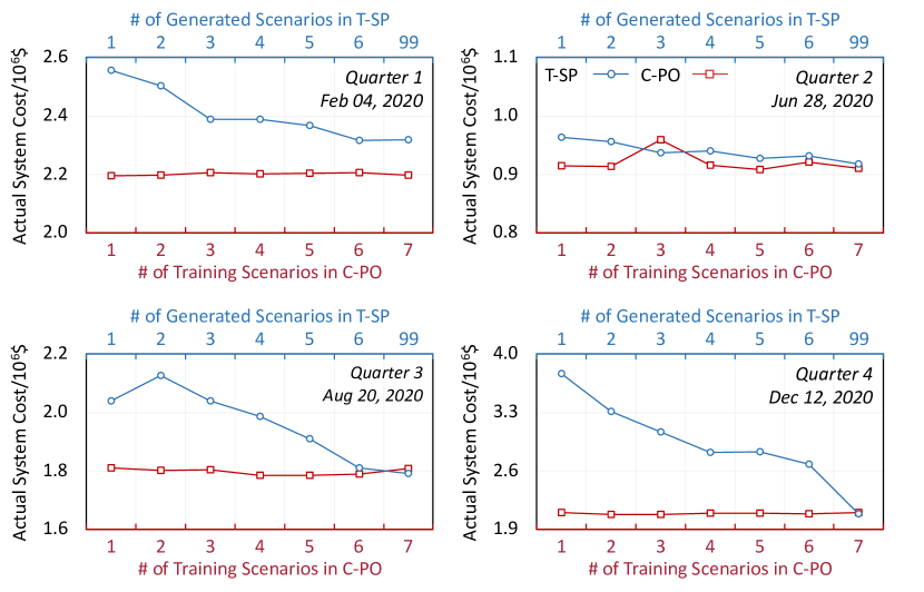
Figure 5: Comparison of C-PO and T-SP.                    

Fig. 5 sketches the operation economics of C-PO and T-SP solutions, leading to the following observations:

• T-SP-NSs require many scenarios to perform well, leaving a wide cost gap between T-SP-1 and T-SP-99. Relatively, C-PO-NTs need fewer scenarios, with a narrower cost gap between C-PO-1 and C-PO-7. It indicates that the bilevel ERM enables C-PO to effectively mine the value of information, ensuring its performance in case of limited scenarios.

• Except for quarter 1, the costs of T-SP-NSs and C-PO-NTs eventually intersect. It implies that the economics of T-SP and C-PO are mutually reachable with suitable $NT$ and $NS$.

• In quarter 1, even with $NS$ = 99, T-SP-NS still performs poorly. This is because the confidence intervals cannot exactly cover the underlying distributions of $\tilde{\boldsymbol{u}}$ and T-SP-NSs would encounter significant slack penalties.

TABLE VII: Breakdown of Actual System Cost on 28 Jun 2020

	Actual UC Cost/$\text{10}^{\text{3}}$$		Hindsight ED Cost/$\text{10}^{\text{3}}$$
	Startup	No-Load	Startup&No-Load	Generation	Slack
C-PO-7	6.7	9.0	0	894.9	0
T-SP-1	6.5	8.1	1.1	934.3	13.7
T-SP-4	5.1	7.7	1.0	926.4	0
T-SP-99	4.8	7.8	0.7	904.7	0

Table VII breaks down the cost on the quarter-2 day. It shows that the T-SP-NSs bring lower startup and no-load costs. This is because the reserve requirements are implicated in (18) rather than being explicit as in (15). Thus, T-SP-NSs turn on fewer units and schedule less reserve in the day-ahead stage, resulting in relatively more extensive usage of quick-start units in the hindsight ED stage. Indeed, our results show that the average hourly reserve schedules (SR plus NR) of T-SP-1 and T-SP-99 are respectively 89.9MW and 207.2MW. In comparison, these average schedules are 1,265.8MW and 1,286.8MW in C-PO-1 and C-PO-7. Moreover, it should be pointed out that as quick-start units have limited ramping ranges, they are operated away from the most efficient points in ED, causing higher generation costs for T-SP-NSs.

Indeed, the difference in reserve schedules implies that T-SP and C-PO achieve similar economics through different ways. Specifically, T-SP schedules fewer reserves and utilizes more RES curtailments in place of SR in actual operation. This may work well in case of ample RES, but becomes economically risky when the actual RES availability is low, as expensive slack penalties will be triggered (e.g., due to insufficient capacity, T-SP-1 is penalized as in Table VII). This could also cause a lower RES utilization, i.e., the RES utilization of T-SP-NSs on the four days is 4.2% lower than C-PO-NTs.

IV-C2 C-PO vs T-RO

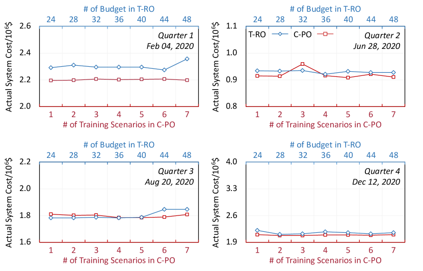
Figure 6: Comparison of C-PO and T-RO.                   

TABLE VIII: Breakdown of Actual System Cost on 20 Aug 2020

	Actual UC Cost/$\text{10}^{\text{3}}$$		Hindsight ED Cost/$\text{10}^{\text{3}}$$
	Startup	No-Load	Startup&No-Load	Generation	Slack
C-PO-7	5.9	12.6	0.2	1789.7	0
T-RO-24	6.5	11.3	1.2	1764.9	0
T-RO-36	6.7	11.4	1.2	1764.3	0
T-RO-48	6.5	11.3	1.2	1764.9	63.5

Fig. 6 sketches the operation economics of C-PO and T-RO. It shows that both methods are relatively stable, i.e., the gap between the best and worst costs is small. Moreover, multiple intersections exist in the curves, implying that T-RO and C-PO could achieve similar economic performance with properly tuned parameters.

Table VIII further compares the costs on the quarter-3 day. It shows that the T-RO-NBs have a higher startup cost but a lower no-load cost in the UC stage. The reason is that T-RO-NBs schedule SR for those hours with potential large volatility, so that multiple units in the UC stage are turned on before these hours and turned off afterward. On the other hand, C-PO-7 constantly keeps more units online to meet the reserve requirements of individual hours, with higher no-load costs. In addition, the penalty of T-RO-48 means that a large $\Gamma$ may not lead to a sufficient reserve schedule. Indeed, the hourly average reserve schedules of T-RO-48 and C-PO-7 are 278.4MW and 1,214.7MW, implying that C-PO-7 is more conservative. With this, it can be pointed out that C-PO achieves similar economics as the state-of-the-art methods in a more reliable way, i.e., schedule more reserves to avoid potential slack penalties.

IV-C3 Discussions

The above comparisons indicate that the operation economics of C-PO is comparable to T-SP and T-RO. Although a clear-cut economic benefit of C-PO is yet to be observed, C-PO does present promising practical advantages.

Computational affordability to system operators: The day-ahead UC to determine optimal operation plans has been widely regarded as one of the most computationally challenging tasks. Concerning that T-SP/T-RO is more computationally taxing than its deterministic counterpart, most system operators still utilize the deterministic UC model (1). In comparison, C-PO is trained offline, and the prescriptive UC model (15) keeps a similar online computation burden as O-PO, thus being more affordable to system operators.

Compatibility with the goal of system operators: In most real-world power systems, the system operators aim to identify the economically optimal UC decisions given the predictions. However, UC decisions of T-SP/T-RO may not fully follow the least-cost principle in the short term due to the uncertainty consideration. Although better operation economics may be reached in the long term, a short-term financial deficit would be unavoidable.

While pursuing to maximize both short- and long-term system economics, the system operators must have a stably interpretable schedule plan (i.e., the operation plan on which units to dispatch) so that both operation plans and post-operation analyses can be effectively conducted. Regarding this, T-SP and T-RO could expose intrinsic obstacles in practical applications. For T-SP, a stable schedule result requires a sufficiently large number of scenarios, which, however, will undoubtedly magnify the existing computational challenge and ultimately end up with a trade-off between the number of scenarios and schedule stability; while for T-RO, subject to the availability of tractable reformulation, uncertainty budget forms are usually designed to be simple, abstract, and heavily parameter-dependent. These together lead to volatility and poor interpretability of schedule results.

Specifically, the scenario generation process (for constructing the scenario set) inevitably introduces randomness. However, different scenario sets, even with tiny differences, may lead to noticeable commitment changes, i.e., those units are committed/decommitted from one set to another. These issues adversely affect the interpretability of the schedule plan. Analogously, uncertainty budget settings will suffer from the same issue. Moreover, an abstract budget lacks a way to be intuitively linked to the scheduling result. That is, the impacts of budget forms and settings on the schedule results are difficult to interpret and quantify. As a result, the system operators have to face the same issue on a daily basis—what is the best budget parameter for the next operation day?

Last but not least, the difference between the scheduled reserves of C-PO and T-SP/T-RO implies that the second stage of T-SP/T-RO may not be able to implicitly secure enough reserves in the UC plan. Hence, the explicit expression of reserve requirements is necessary for the UC model.

In comparison, the prescriptive UC (15) has the same model structure as (1), thus following the least-cost principle and remaining strong interpretability. In addition, the results have clearly shown that efficiencies of T-SP/T-RO and C-PO are mutually reachable. Therefore, it is promising to harness the compatibility of C-PO in bridging the gap between the state-of-the-art T-SP/T-RO and the current practice.

V Conclusion

This paper proposes a bilevel MIP-based C-PO framework for improving the operation economics as compared to the traditional O-PO framework. The idea is to leverage the bilevel MIP structure to train the cost-oriented RES and reserve predictors to be integrated into the optimal operation task, in which the prediction quality is evaluated via operation costs. Case studies lead to the following conclusions:

• Benefiting from the bilevel MIP structure, C-PO can economically outperform traditional O-PO with limited training scenarios. According to the results of selective weeks in different seasons, C-PO with 7 training scenarios can lead to a 2.54% improvement in daily operation economics on average, even though the cost-oriented RES predictions present slightly worse MAEs and RMSEs.

• The operation economics of C-PO, T-SP, and T-RO could be mutually reachable, with sufficient scenarios for T-SP and comprehensively tuned parameters for T-RO. Nevertheless, given its high compatibility with the current power system operation practice, C-PO presents higher implementation values to serve as a bridge between T-SP/T-RO-based UC and the current deterministic UC practice.

Future work could focus on accelerating the training process of C-PO to further boost its implementation in power system practice.

-A Deterministic UC Model

The objective (20a) is to minimize the total system cost, including startup, no-load, and generation costs. The generator constraints include generation limits (20b), segment-based generation representation (20c)-(20d), SR (20e) and NR (20f) capacity limits, startup-shutdown-commitment status logic (20g), minimum on and off requirements (20h)-(20i), ramping limits (20j), and RES power limitation (20k). Constraints (20l)-(20m) mean that offline non-quick-start units cannot provide NR. Constraint (20n) is the integrality requirement. System constraints include power balance (20o), DC power flow-based transmission limits (20p) [4], and system reserve requirements (20q).

$$\min\textstyle{\sum\limits_{t\in\mathcal{T},i\in\mathcal{I}}}(\textstyle{C_{i}^{su}U_{it}+C_{i}^{nl}I_{it}+\sum\limits_{k\in\mathcal{K}}C^{sg}_{ik}P_{itk}^{sg})}$$ (20a)

Generator Constraints:

$$\textstyle{P_{it}-R_{it}^{sr}\geq\underline{P\mkern-6.0mu}\mkern 4.0mu_{i}I_{it}};\,\textstyle{P_{it}+R_{it}^{sr}\leq\bar{P}_{i}I_{it}}; \mspace{-197.0mu}\textstyle{\forall t\in\mathcal{T},i\in\mathcal{I}}$$ (20b)

$$\textstyle{P_{it}=\sum_{k\in\mathcal{K}}P_{itk}^{sg}}; \mspace{-199.0mu}\textstyle{\forall t\in\mathcal{T},i\in\mathcal{I}}$$ (20c)

$$\textstyle{0\leq P_{itk}^{sg}\leq\bar{P}_{ik}^{sg}I_{it}}; \mspace{-199.0mu}\textstyle{\forall t\in\mathcal{T},i\in\mathcal{I},k\in\mathcal{K}}$$ (20d)

$$\textstyle{0\leq R_{it}^{sr}\leq\bar{R}_{i}^{sr}I_{it}}; \mspace{-199.0mu}\textstyle{\forall t\in\mathcal{T},i\in\mathcal{I}}$$ (20e)

$$\textstyle{\underline{P\mkern-6.0mu}\mkern 4.0mu_{i}O_{it}\leq R_{it}^{nr}\leq\bar{R}_{i}^{nr}O_{it}}; \mspace{-199.0mu}\textstyle{\forall t\in\mathcal{T},i\in\mathcal{I}}$$ (20f)

$$\textstyle{U_{it}-D_{it}=I_{it}-I_{i,t-1}}; \mspace{-199.0mu}\textstyle{\forall t\in\mathcal{T},i\in\mathcal{I}}$$ (20g)

$$\textstyle{\sum_{t^{\prime}=t-T_{i}^{su}+1}^{t}U_{it^{\prime}}\leq I_{it}}; \mspace{-199.0mu}\textstyle{\forall t\in\mathcal{T}^{su}_{i},i\in\mathcal{I}}$$ (20h)

$$\textstyle{\sum_{t^{\prime}=t-T_{i}^{sd}+1}^{t}D_{it^{\prime}}\leq 1-I_{it}}; \mspace{-199.0mu}\textstyle{\forall t\in\mathcal{T}^{sd}_{i},i\in\mathcal{I}}$$ (20i)

$$\textstyle{P_{it}-P_{i,t-1}\leq\bar{P}_{i}(1-I_{it})+R_{i}^{\uparrow}I_{i,t-1}+R_{i}^{su}(I_{it}-I_{i,t-1})};\,\,$$

$$\textstyle{P_{i,t-1}-P_{it}\leq\bar{P}_{i}(1-I_{i,t-1})+R^{\downarrow}_{i}I_{it}+R^{sd}_{i}(I_{i,t-1}-I_{it})};$$

$$\mspace{-199.0mu}\textstyle{\forall t\in\mathcal{T},i\in\mathcal{I}}$$ (20j)

$$\textstyle{0\leq W_{jt}\leq\hat{{W}}_{jt}}; \mspace{-199.0mu}\textstyle{\forall t\in\mathcal{T},j\in\mathcal{J}}$$ (20k)

$$\textstyle{O_{it}+I_{it}\leq 1}; \mspace{-199.0mu}\textstyle{\forall t\in\mathcal{T},i\in\mathcal{I}}$$ (20l)

$$\textstyle{O_{it}=0}; \mspace{-199.0mu}\textstyle{\forall t\in\mathcal{T},i\in\mathcal{I}^{ns}}$$ (20m)

$$\textstyle{I_{it},U_{it},D_{it},O_{it}\in\{0,1\}}; \mspace{-199.0mu}\textstyle{\forall t\in\mathcal{T},i\in\mathcal{I}}$$ (20n)

System Constraints:

$$\textstyle{\sum\nolimits_{i\in\mathcal{I}}P_{it}+\sum\nolimits_{j\in\mathcal{J}}W_{jt}=\sum\nolimits_{q\in\mathcal{Q}}\hat{L}_{qt}}; \mspace{-199.0mu}\textstyle{\forall t\in\mathcal{T}}$$ (20o)

$$\textstyle{-B_{b}\leq\mathcal{F}_{b}(P_{it},W_{jt},\hat{L}_{qt})\leq B_{b}}; \mspace{-199.0mu}\textstyle{\forall t\in\mathcal{T},b\in\mathcal{B}}$$ (20p)

$$\textstyle{\sum_{i\in\mathcal{I}}R_{it}^{sr}\mspace{-3.0mu}\geq\mspace{-3.0mu}\hat{R}_{t}^{sr}};\,\,\textstyle{\sum_{i\in\mathcal{I}}(R_{it}^{sr}+R_{it}^{nr})\mspace{-3.0mu}\geq\mspace{-3.0mu}\hat{R}_{t}^{sr}\mspace{-3.0mu}+\mspace{-3.0mu}\hat{R}_{t}^{nr}}; \mspace{-110.0mu}\textstyle{\forall t\in\mathcal{T}}$$ (20q)

-B Hindsight ED Model

The objective (21c) is to minimize startup and no-load costs of quick-start units that are not committed in UC but scheduled for providing NR, generation costs of all units, and slack penalty costs. Constraints (21d)-(21e) mean that only the quick-start units not committed in UC may change statuses. All units are subjected to generation limits (21f)-(21h), dispatch adjustment limits (21i), ramping limits (21j), RES power limits (21k), and integrality requirement (21l). The system shall satisfy power balance (21m) and transmission limits (21n)-(21o) against actual load and RES realizations. Slack variables $\boldsymbol{S}^{1/2/3/4}$ are used to ensure ED feasibility with respect to the given UC solutions.

$$\min\mspace{-5.0mu}\textstyle{\sum\limits_{t\in\mathcal{T}}}\mspace{-5.0mu}\left\{\mspace{-5.0mu}\begin{array}[]{l}\textstyle{\sum\limits_{i\in\mathcal{I}}(C_{i}^{su}U_{it}^{ed,qs}+C_{i}^{nl}I_{it}^{ed,qs}+\sum\limits_{k\in\mathcal{K}}C_{ik}^{sg}P_{itk}^{ed,sg}})\\ \textstyle{+[C^{1}S_{t}^{1}+C^{2}S_{t}^{2}+C^{bs}\sum\nolimits_{b\in\mathcal{B}}(S_{bt}^{3}+S_{bt}^{4})]}\end{array}\right\}\mspace{-24.0mu}$$ (21c)

Generator Constraints:

$$\textstyle{I_{it}^{ed}=I_{it}^{\star}+I_{it}^{ed,qs}};\,\,\textstyle{I_{it}^{ed,qs}\leq O_{it}^{\star}}; \mspace{-200.0mu}\textstyle{\forall t\in\mathcal{T},i\in\mathcal{I}}$$ (21d)

$$\textstyle{U_{it}^{ed,qs}-D_{it}^{ed,qs}=I_{it}^{ed,qs}-I_{i,t-1}^{ed,qs}}; \mspace{-200.0mu}\textstyle{\forall t\in\mathcal{T},i\in\mathcal{I}}$$ (21e)

$$\textstyle{P_{it}^{ed}=\sum\nolimits_{k\in\mathcal{K}}P_{itk}^{ed,sg}}; \mspace{-200.0mu}\textstyle{\forall t\in\mathcal{T},i\in\mathcal{I}}$$ (21f)

$$\textstyle{0\leq P_{itk}^{ed,sg}\leq\bar{P}_{ik}^{sg}I_{it}^{ed}}; \mspace{-200.0mu}\textstyle{\forall t\in\mathcal{T},i\in\mathcal{I},k\in\mathcal{K}}$$ (21g)

$$\textstyle{P_{it}^{ed}\geq\underline{P\mkern-6.0mu}\mkern 4.0mu_{i}I_{it}^{ed}};\,\,\textstyle{P_{it}^{ed}\leq\bar{P}_{i}I_{it}^{\star}+R_{it}^{nr\star}I_{it}^{ed,qs}}; \mspace{-145.0mu}\textstyle{\forall t\in\mathcal{T},i\in\mathcal{I}}$$ (21h)

$$\textstyle{-R_{it}^{sr\star}I_{it}^{\star}\leq P_{it}^{ed}-P_{it}^{\star}\leq R_{it}^{sr\star}I_{it}^{\star}+\bar{P}_{i}I_{it}^{ed}}; \mspace{-145.0mu}\textstyle{\forall t\in\mathcal{T},i\in\mathcal{I}}$$ (21i)

$$\textstyle{P_{it}^{ed}-P_{i,t-1}^{ed}\leq\bar{P}_{i}(1-I_{it}^{ed})+R_{i}^{\uparrow}I_{i,t-1}^{ed}+R_{i}^{su}(I_{it}^{ed}-I_{i,t-1}^{ed})};$$

$$\textstyle{P_{i,t-1}^{ed}-P_{it}^{ed}\leq\bar{P}_{i}(1-I_{i,t-1}^{ed})+R^{\downarrow}_{i}I_{it}^{ed}+R^{sd}_{i}(I_{i,t-1}^{ed}-I_{it}^{ed})};$$

$$\mspace{-200.0mu}\textstyle{\forall t\in\mathcal{T},i\in\mathcal{I}}$$ (21j)

$$\textstyle{0\leq W_{jt}^{ed}\leq\tilde{{W}}_{jt}}; \mspace{-200.0mu}\textstyle{\forall t\in\mathcal{T},j\in\mathcal{J}}$$ (21k)

$$\textstyle{I_{it}^{ed},I_{it}^{ed,qs},U_{it}^{ed,qs},D_{it}^{ed,qs}\in\{0,1\}}; \mspace{-200.0mu}\textstyle{\forall t\in\mathcal{T},i\in\mathcal{I}}$$ (21l)

System Constraints:

$$\textstyle{\sum\limits_{i\in\mathcal{I}}\mspace{-5.0mu}P_{it}^{ed}+\mspace{-5.0mu}\sum\limits_{j\in\mathcal{J}}\mspace{-5.0mu}W_{jt}^{ed}+\mspace{-3.0mu}S_{t}^{1}=\mspace{-5.0mu}\sum\limits_{q\in\mathcal{Q}}\mspace{-5.0mu}\tilde{L}_{qt}+\mspace{-3.0mu}S_{t}^{2}};\,\textstyle{S_{t}^{1},S_{t}^{2}\geq 0}; \mspace{-95.0mu}\textstyle{\forall t\in\mathcal{T}}$$ (21m)

$$\textstyle{\mathcal{F}_{b}(P_{it}^{ed},W_{jt}^{ed},\tilde{L}_{qt})-S_{bt}^{3}\leq B_{b}};\,\,\textstyle{S_{bt}^{3}\geq 0}; \mspace{-150.0mu}\textstyle{\forall t\in\mathcal{T},b\in\mathcal{B}}$$ (21n)

$$\textstyle{\mathcal{F}_{b}(P_{it}^{ed},W_{jt}^{ed},\tilde{L}_{qt})+S_{bt}^{4}\geq-B_{b}};\,\,\textstyle{S_{bt}^{4}\geq 0}; \mspace{-150.0mu}\textstyle{\forall t\in\mathcal{T},b\in\mathcal{B}}$$ (21o)

-C Proof of Proposition 1

Proof:

To prove Proposition 1, problem (22) is built to serve as a bridge between (9) and (11), which is constructed by adding (22d) to (9) or adding (22f) to (11).

$$\textstyle{\min_{\mathcal{W},\mathcal{R}}} \mspace{-30.0mu}\textstyle{\frac{1}{|\mathcal{S}|}\sum\nolimits_{s\in\mathcal{S}}}(\boldsymbol{b}^{\top}\boldsymbol{x}_{s}+\boldsymbol{d}^{\top}\boldsymbol{z}_{s})$$ (22a)

$$s.\,t.\, \mspace{-70.0mu}\mathcal{W}(\cdot)\in\mathcal{P}^{w};\,\,\mathcal{R}(\cdot)\in\mathcal{P}^{r}$$ (22b)

$$\mspace{-70.0mu}\hat{\boldsymbol{w}}^{\diamond}_{s}=\mathcal{W}(\boldsymbol{f}^{w}_{s});\,\,\hat{\boldsymbol{r}}^{\diamond}_{s}=\mathcal{R}(\boldsymbol{f}^{r}_{s}); \mspace{-30.0mu}\forall s\in\mathcal{S}$$ (22c)

$$\mspace{-70.0mu}\boldsymbol{z}_{s}\in\mathcal{Z}(\boldsymbol{x}_{s},\boldsymbol{y}_{s},\tilde{\boldsymbol{w}}_{s}); \mspace{-30.0mu}\forall s\in\mathcal{S}$$ (22d)

$$\mspace{-70.0mu}\boldsymbol{x}_{s},\boldsymbol{y}_{s}\in{\arg\min}_{\boldsymbol{x}_{s},\boldsymbol{y}_{s}\in\mathcal{X}(\hat{\boldsymbol{w}}^{\diamond}_{s},\hat{\boldsymbol{r}}^{\diamond}_{s})}\boldsymbol{b}^{\top}\boldsymbol{x}_{s}+\boldsymbol{c}^{\top}\boldsymbol{y}_{s}; \mspace{-30.0mu}\forall s\in\mathcal{S}$$ (22e)

$$\mspace{-70.0mu}\boldsymbol{z}_{s}\in{\arg\min}_{\boldsymbol{z}_{s}\in\mathcal{Z}(\boldsymbol{x}_{s},\boldsymbol{y}_{s},\tilde{\boldsymbol{w}}_{s})}\boldsymbol{d}^{\top}\boldsymbol{z}_{s}; \mspace{-30.0mu}\forall s\in\mathcal{S}$$ (22f)

First, we claim that (9) and (22) have the same optimal solutions because their objective functions are identical and their feasible regions are also the same. They have the same feasible regions because (i) A feasible solution of (9) satisfies all constraints of (22) and thus is feasible to (22); and (ii) A feasible solution of (22) also meets all constraints of (9) and thus is feasible to (9). Thus, (9) and (22) have the same optimal solutions.

Second, we claim that the optimal solution of (11) is also optimal for (22). Note that as (11) is equivalent to (22a)-(22e), we only need to show that the optimal solution of (11) also satisfies (22f). Specifically, if $\Omega^{\star}$ (including $\boldsymbol{x}_{s}^{\star}$, $\boldsymbol{y}_{s}^{\star}$, and $\boldsymbol{z}_{s}^{\star}$) is an optimal solution of (11), $\boldsymbol{z}^{\star}_{s}$ must be optimal for (23) that is constructed by fixing all variables in (11) to their optima except $\boldsymbol{z}_{s}$. Problem (23) is equivalent to (22f), i.e., $\boldsymbol{z}^{\star}_{s}$ satisfies (22f). Thus, because $\Omega^{\star}$ is optimal for (22a)-(22e) and its $\boldsymbol{z}^{\star}_{s}$ also satisfies (22f), $\Omega^{\star}$ must be optimal for (22).

$$\textstyle{\min_{\boldsymbol{z}_{s}}} \mspace{-35.0mu}\textstyle{\frac{1}{|\mathcal{S}|}\sum\nolimits_{s\in\mathcal{S}}}(\boldsymbol{b}^{\top}\boldsymbol{x}_{s}^{\star}+\boldsymbol{d}^{\top}\boldsymbol{z}_{s})$$ (23a)

$$s.\,t. \mspace{-35.0mu}\textstyle{\boldsymbol{z}_{s}\in{\arg\min}_{\boldsymbol{z}_{s}\in\mathcal{Z}(\boldsymbol{x}^{\star}_{s},\boldsymbol{y}^{\star}_{s},\tilde{\boldsymbol{w}}_{s})}\boldsymbol{d}^{\top}\boldsymbol{z}_{s}};\quad\forall s\in\mathcal{S}$$ (23b)

From the above claims, it is direct to conclude that the optimal solution of (11) is optimal for (22), and thus also optimal for (9). ∎

References

- [1] W. Wei, F. Liu, and S. Mei, “Distributionally robust co-optimization of energy and reserve dispatch,” IEEE Trans. Sustain. Energy, vol. 7, no. 1, pp. 289–300, 2016.
- [2] M. Parvania and M. Fotuhi-Firuzabad, “Demand response scheduling by stochastic SCUC,” IEEE Trans. Smart Grid, vol. 1, no. 1, pp. 89–98, 2010.
- [3] T. Ding, R. Bo, W. Gu, Q. Guo, and H. Sun, “Absolute value constraint based method for interval optimization to SCED model,” IEEE Trans. Power Syst., vol. 29, no. 2, pp. 980–981, 2014.
- [4] L. Wu, M. Shahidehpour, and T. Li, “Stochastic security-constrained unit commitment,” IEEE Trans. Power Syst., vol. 22, no. 2, pp. 800–811, 2007.
- [5] B. Hu and L. Wu, “Robust SCUC considering continuous/discrete uncertainties and quick-start units: A two-stage robust optimization with mixed-integer recourse,” IEEE Trans. Power Syst., vol. 31, no. 2, pp. 1407–1419, 2016.
- [6] D. Bertsimas and N. Kallus, “From predictive to prescriptive analytics,” Manage. Sci., vol. 66, no. 3, pp. 1025–1044, 2020.
- [7] A. N. Elmachtoub and P. Grigas, “Smart “predict, then optimize”,” Manage. Sci., vol. 68, no. 1, pp. 9–26, 2022.
- [8] G.-Y. Ban and C. Rudin, “The big data newsvendor: Practical insights from machine learning,” Oper. Res., vol. 67, no. 1, pp. 90–108, 2019.
- [9] G. Li and H.-D. Chiang, “Toward cost-oriented forecasting of wind power generation,” IEEE Trans. Smart Grid, vol. 9, no. 4, pp. 2508–2517, 2018.
- [10] A. C. Stratigakos, S. Camal, A. Michiorri, and G. Kariniotakis, “Prescriptive trees for integrated forecasting and optimization applied in trading of renewable energy,” IEEE Trans. Power Syst., pp. 1–1, 2022.
- [11] T. Carriere and G. Kariniotakis, “An integrated approach for value-oriented energy forecasting and data-driven decision-making application to renewable energy trading,” IEEE Trans. Smart Grid, vol. 10, no. 6, pp. 6933–6944, 2019.
- [12] J. Han, L. Yan, and Z. Li, “A task-based day-ahead load forecasting model for stochastic economic dispatch,” IEEE Trans. Power Syst., vol. 36, no. 6, pp. 5294–5304, 2021.
- [13] Y. Zhang, H. Wen, and Q. Wu, “A contextual bandit approach for value-oriented prediction interval forecasting,” arXiv:2210.04152, 2023.
- [14] L. Sang, Y. Xu, H. Long, Q. Hu, and H. Sun, “Electricity price prediction for energy storage system arbitrage: A decision-focused approach,” IEEE Trans. Smart Grid, vol. 13, no. 4, pp. 2822–2832, 2022.
- [15] C. Zhao, C. Wan, and Y. Song, “Operating reserve quantification using prediction intervals of wind power: An integrated probabilistic forecasting and decision methodology,” IEEE Trans. Power Syst., vol. 36, no. 4, pp. 3701–3714, 2021.
- [16] M. A. Muñoz, J. M. Morales, and S. Pineda, “Feature-driven improvement of renewable energy forecasting and trading,” IEEE Trans. Power Syst., vol. 35, no. 5, pp. 3753–3763, 2020.
- [17] J. M. Morales, M. Á. Muñoz, and S. Pineda, “Value-oriented forecasting of net demand for electricity market clearing,” arXiv:2108.01003, 2021.
- [18] X. Chen, Y. Yang, Y. Liu, and L. Wu, “Feature-driven economic improvement for network-constrained unit commitment: A closed-loop predict-and-optimize framework,” IEEE Trans. Power Syst., vol. 37, no. 4, pp. 3104–3118, 2022.
- [19] C. Zhao, C. Wan, and Y. Song, “Cost-oriented prediction intervals: On bridging the gap between forecasting and decision,” IEEE Trans. Power Syst., vol. 37, no. 4, pp. 3048–3062, 2022.
- [20] M. Muñoz, S. Pineda, and J. Morales, “A bilevel framework for decision-making under uncertainty with contextual information,” Omega, vol. 108, p. 102575, 2022.
- [21] J. D. Garcia, A. Street, T. Homem-de Mello, and F. D. Muñoz, “Application-driven learning via joint prediction and optimization of demand and reserves requirement,” arXiv:2102.13273, 2021.
- [22] V. Dvorkin, S. Delikaraoglou, and J. M. Morales, “Setting reserve requirements to approximate the efficiency of the stochastic dispatch,” IEEE Trans. Power Syst., vol. 34, no. 2, pp. 1524–1536, 2019.
- [23] N. Viafora, S. Delikaraoglou, P. Pinson, G. Hug, and J. Holbøll, “Dynamic reserve and transmission capacity allocation in wind-dominated power systems,” IEEE Trans. Power Syst., vol. 36, no. 4, pp. 3017–3028, 2021.
- [24] B. Zeng and Y. An, “Solving bilevel mixed integer program by reformulations and decomposition,” Optim. Online, 2014.
- [25] (2022). [Online]. Available: github.com/asxadf/Bilevel_MIP_CPO.
- [26] (2022). [Online]. Available: opendata.elia.be/pages/home.
- [27] Y. Zhang, X. Zhang, P. Huang, and Y. Sun, “Global sensitivity analysis for key parameters identification of net-zero energy buildings for grid interaction optimization,” Appl. Energy, vol. 279, p. 115820, 2020.
- [28] S. Pineda and J. M. Morales, “Solving linear bilevel problems using Big-Ms: Not all that glitters is gold,” IEEE Trans. on Power Syst., vol. 34, no. 3, pp. 2469–2471, 2019.
- [29] J. Löfberg, “YALMIP: A toolbox for modeling and optimization in MATLAB,” in In Proceedings of the CACSD Conference, Taipei, Taiwan, 2004.
- [30] J. Dupačová, N. Gröwe-Kuska, and W. Römisch, “Scenario reduction in stochastic programming,” Math. Program., vol. 95, no. 3, pp. 493–511, 2003.
- [31] L. Zhao and B. Zeng, “An exact algorithm for two-stage robust optimization with mixed integer recourse problems,” Optim. Online, 2012.