Dynamics of composite symplectic Dehn twists

Abstract.

This paper appears as the confluence of hyperbolic dynamics, symplectic topology and low dimensional topology, etc. We show that composite symplectic Dehn twists have certain form of nonuniform hyperbolicity that can be used to give positive topological entropy as well as two families of local stable and unstable Lagrangian manifolds, as signatures of pseudo Anosov mapping classes. Moreover, we also show that the rank of the Floer cohomology group grows exponentially under iterations.

1. Introduction

In this paper, we study the dynamical behaviors of elements in the symplectic mapping class group of a symplectic manifold. When the symplectic manifold is a surface, the classical Nielson-Thurston theory gives important understanding of the dynamics of the mapping classes: every automorphism $f$ of $S$ is homotopic to a homeomorphism $\phi$ that satisfies one of the following, periodic ($\phi^{k}=\mathrm{id}$ for some $k\in\mathbb{N}$), reducible (there exists a closed loop $\gamma\subset S$ preserved by $\phi$) and pseudo-Anosov, featured by the following two properties, among others:

1. Existence of two singular transversal foliations invariant under a representative element of the mapping class;

2. Expansion/contraction along the leaves, measured by positive topological entropy.

Pseudo Anosov mapping classes are particularly interesting to us. They are natural generalization of Anosov systems which are central objects studied in hyperbolic dynamical systems. Moreover, they constitute most of the classes in the mapping class group.

To see the ideas clearer, let us consider the torus case. Consider the linear automorphisms in $\mathrm{PSL}_{2}\mathbb{Z}=\mathrm{SL}_{2}\mathbb{Z}/\{\pm\mathrm{id}\}$ acting on the torus $\mathbb{R}^{2}/\mathbb{Z}^{2}$. An automorphism $f$ in $\mathrm{PSL}_{2}\mathbb{Z}$ falls into one of the three types:

1. $\mathrm{tr}(f)<2$, $f$ is periodic, and $f^{k}=\mathrm{id}$ for some $k\in\mathbb{N}$;

2. $\mathrm{tr}(f)=2$, $f$ is reducible, and $f$ has linear growth;

3. $\mathrm{tr}(f)>2$, $f$ is Anosov, and $f$ expands in one eigen-direction while contracts in the other.

A classical example of Anosov automorphism is given by the Arnold’s cat map: $f=\begin{pmatrix}2&1\\ 1&1\end{pmatrix}$. We see that it can be written as a composition of upper and lower triangular matrices $\begin{pmatrix}1&1\\ 0&1\end{pmatrix}$ and $\begin{pmatrix}1&0\\ 1&1\end{pmatrix}$, which are examples of Dehn twists on the torus given by cutting the surface along a closed curve, twisting a tubular neighborhood of one side of the curve by $2\pi$ and gluing the curve back together.

More generally, composing of Dehn twists is a standard procedure of producing pseudo Anosov elements. The algorithm can be found in the work of Thurston [32], Penner [25], Fathi [13], et al.

It was noted in [2] that “the natural generalization of $\mathrm{SL}(2)$ is from many points of view not $\mathrm{SL}(n)$ but rather the linear symplectomorphisms group $\mathrm{Sp}(n)$ of $2n$-space and correspondingly the group Symp$(M)$”. For $2n$-dimensional symplectic manifolds with $n>1$, we also have the generalization of Dehn twists by Arnold [2] and Seidel [29]: if $L$ is a Lagrangian sphere on a symplectic manifold $M$, the Dehn twist $\tau_{L}$ with respect to $L$ acts on $M$ roughly by twisting a tubular neighborhood of $L$ so that $L$ is identified with itself via the antidopal map (See Definition 2.1 for the precise statement). Unlike the case of Dehn twists on surfaces, for which the Dehn twist represents a nontrivial mapping class, the symplectic Dehn twist $\tau^{2}_{L}$ is in fact homotopic to the identity, but represents a nontrivial symplectic mapping class [29].

We thus expect that by composing symplectic Dehn twists we can get symplectic mapping classes having features of pseudo Anosov mapping classes. We are interested in revealing hyperbolicity of such elements, hence proving properties analogous to the above items (a) and (b) (see Theorem 1.1, 1.2, 1.3 below). We will also study the exponential growth of ranks of Floer cohomology groups of these elements (see Theorem 1.4 and 1.5 below). Moreover, we will also discuss the complexity of the dynamics by comparing it with the standard map.

The composite symplectic Dehn twists has been recently studied by many authors from the perspective of categorical dynamics. We refer readers to [5, 11, 21] and more references therein.

1.1. Positive topological entropy

We first show that certain natural representatives of compositions of symplectic Dehn twists have positive topological entropy.

Theorem 1.1.

Let $S_{1}$ and $S_{2}$ be two Lagrangian spheres in a symplectic manifold $M$, intersecting transversely at a single point. Then there exist symplectic Dehn twists $\tau_{1}$ and $\tau_{2}$ of $S_{1}$ and $S_{2}$, such that for any $k,\ell\in\mathbb{Z},k\ell<0$, the topological entropy of the composition $\tau=\tau_{1}^{k}\tau_{2}^{\ell}$ of symplectic Dehn twists is positive, i.e. $h_{top}(\tau_{1}^{k}\tau_{2}^{\ell})>0.$

In case there are more than two Lagrangian spheres, a natural setting is $A_{m}$ configurations that was studied intensively in literature. It is known that its symplectic mapping class group is generated by symplectic Dehn twists [33]. We shall describe it in Example 2.2.1 following [29].

Theorem 1.2.

Let $S_{i},1\leq i\leq m$ be the $m$ embedded Lagrangian spheres in $A_{m}$ as given in Example 2.2.1, there exist Dehn twists $\tau_{i}$ on $S_{i}$ for each $1\leq i\leq m$ such that for any $k_{i}\in\mathbb{Z}$ such that $k_{i}k_{i+1}<0$ for all $i=1,2,\ldots,m-1$, the topological entropy of $\tau=\tau_{1}^{k_{1}}\cdots\tau_{m}^{k_{m}}$ is positive, i.e.

$$h_{top}(\tau_{1}^{k_{1}}\cdots\tau_{m}^{k_{m}})>0.$$

The proof of the theorem is to find an invariant submanifold on which the dynamics is hyperbolic, i.e. with positive Lyapunov exponent on a positive two dimensional Lebesgue measure set. The positive topological entropy follows from the variational equation as well as Pesin entropy formula. The origin of the hyperbolicity of Theorem 1.1 is that the subsystem is modeled on an object that is similar to the linked twist map studied intensively in literature (see [8]). The linked twist map was used by Polterovich and Shelukhin in [27] to exhibit an example of Hamiltomorphism that is far from autonomous ones or powers. For Theorem 1.2, we introduce a more complicated version of linked twist map that we call multi-linked twist map.

As a corollary of the proof of the last theorems, we also show that these compositions of Dehn twists admit a pair of local stable/unstable Lagrangian manifolds.

Theorem 1.3.

In the setting of the Theorem 1.1 and Theorem 1.2, there exist two families of Lagrangian submanifolds $\mathcal{F}^{s},\mathcal{F}^{u}$ on $M$ in a neighbourhood $N$ of $\cup S_{i}$ which are invariant under $\tau$. Furthermore, there is an invariant subset $P$ of $N$ admitting an $\mathrm{SO}(n)$ action that commutes with $\tau$ and preserves each leaf in $\mathcal{F}^{s}$ and $\mathcal{F}^{u}$, such that

1. $P/\mathrm{SO}(n)$ is a two dimensional manifold with boundary,

2. either of $\mathcal{F}^{s}/\mathrm{SO}(n)$ and $\mathcal{F}^{u}/\mathrm{SO}(n)$ has full Lebesgue measure on $P/\mathrm{SO}(n)$

3. for a.e. $x\in P/\mathrm{SO}(n)$, the leaf $f^{s}(x)$ $($resp. $f^{u}(x))$ of $\mathcal{F}^{s}/\mathrm{SO}(n)$ $($resp. $\mathcal{F}^{u}/\mathrm{SO}(n))$ passing through $x$ is contracted exponentially under iterations of $\tau$ $($resp. $\tau^{-1})$.

This follows from Pesin’s stable manifold theorem (Theorem A.4). Finding symplectic diffeomorphisms admitting stable/unstable laminations was asked in [10] as an open problem. The problem was studied in [23] which constructed train tracks using ideas from Penner [25] by smoothing the corners of two transversally intersecting Lagrangian submanifolds. There are further standard consequences from nonuniformly hyperbolic dynamics such as existence of horseshoe on $P/\mathrm{SO}(n)$ conjugating to Bernoulli shifts, hence exponentially growth of periodic orbits, etc, for which we refer readers to Chapter S. 5 of [19].

1.2. Exponential growth of the rank of Floer homology groups

The above results rely on a particular choice of a representative in the symplectic mapping classes, as in the Nielson-Thurston theory, so the results are in general not robust under perturbations. On the other hand, the symplectic nature of the problem makes it also natural and necessary to describe the complexity of the dynamics in terms of symplectic invariants, which is not sensitive to the choice of a representative in the symplectic mapping classes. It is then important and natural to study the growth of symplectic invariants such as Floer cohomology of $\mathrm{HF}(S_{1},\tau^{n}S_{2})$ for $\tau$ as above.

Definition 1.1 (Symplectic growth rate).

Let $(M,\omega)$ be a symplectic manifold, and $\phi$ a symplectomorphism of $M$. Let $(L_{1},L_{2})$ be a pair of connected compact Lagrangian submanifolds of $M$. When the Lagrangian Floer cohomology group $\mathrm{HF}(L_{1},\phi^{n}(L_{2}))$ are well defined for all $n\in\mathbb{N}$, then the symplectic growth rate of the triple $(\phi,L_{1},L_{2})$ is defined by

$$\Gamma(\phi,L_{1},L_{2})=\liminf_{n\to\infty}\frac{\log\mathrm{rank}\;\mathrm{HF}(L_{1},\phi^{n}(L_{2}))}{n}.$$

The work of Arnold and Seidel [3, 31] tells us that the above growth rate (whenever it is defined) has uniform bound which only depends on $M$ and $\phi$, explicitly, given $\phi\in\mathrm{Symp}(M,\omega)$, for any Lagrangian submanifolds $L_{1}$ and $L_{2}$, there is a constant $C$ such that

$$\mathrm{rank}\;\mathrm{HF}(L_{1},\phi^{n}(L_{2}))\leq C\|D\phi\|^{n\;dim(M)}\quad\hbox{for all $n$}.$$

We next show that the exponential growth can actually be achieved by composite symplectic Dehn twists.

Theorem 1.4.

Let $M$ be an exact symplectic manifold which is equal to a symplectization of a contact manifold near infinity. Let $S_{1}$ and $S_{2}$ be two Lagrangian spheres of $M$ intersecting transversely at a single point, and $\tau_{1}$ and $\tau_{2}$ be two symplectic Dehn twists along the spheres $S_{1}$ and $S_{2}$ respectively. Then

1. for any $k,\ell\in\mathbb{Z}$ with $k\ell\neq 0,1,2,3,4,$ we have that $\Gamma(\tau_{1}^{k}\tau_{2}^{\ell},S_{1},S_{2})>0$;

2. for any $k,\ell\in\mathbb{Z}$ with $k\ell\in\{0,1,2,3,4\}$ we have $\Gamma(\tau_{1}^{k}\tau^{\ell}_{2},S_{1},S_{2})=0$;

3. for $i,j\in\{1,2\}$ with $i\neq j$ we have $\Gamma(\tau_{i}^{2},S_{j},S_{j})=0$.

Although the symplectic growth rate in case (3) of the above theorem is zero, it can be shown that the rank of $\mathrm{HF}(S_{j},\tau_{i}^{2n}(S_{j}))$ grows with polynomial rate, see Section 6.1. Using a similar computation of the rank of Lagrangian Floer homology one can show that the slow volume growth of the symplectic Dehn twist on the cotangent bundle $T^{*}\mathbb{S}^{d}$ of $d$-sphere is positive, see [17]. In [4], the authors develop a categorical machinery which can be used to yield similar but different exponential growth results.

More generally for $A_{m}$-type configuration, we have the following.

Theorem 1.5.

Let $S_{i},1\leq i\leq m,$ be the $m$ embedded Lagrangian spheres in $A_{m}^{n}$-configuration of Lagrangian n-spheres as given in Example 2.2.1, and $\tau_{i}$, $i=1,\ldots,m$ be the symplectic Dehn twist along $n$-spheres $S_{i}$ respectively. Let $\tau=\tau_{1}^{k_{1}}\cdots\tau_{m}^{k_{m}}$ with each $k_{i}\in\mathbb{Z}\setminus\{0\}$ and $k_{i}\cdot k_{i+1}<0$ for all $i=1,\ldots,m-1$.Then we have $\Gamma(\tau,S_{k},S_{\ell})>0$ for all $k,\ell\in\{1,\ldots,m\}$ with $k\neq\ell$.

The last two results are proved by combining the machinery of [22] and classical theory on mapping class groups of surfaces. The last theorem can be considered as an analogue of Theorem 3.1 of [25].

1.3. Speculations on the complexity of the dynamics of composite Dehn twists

It is important to point out that the above study does not reveal all the complexity of the dynamics of composite symplectic Dehn twists. In this section and Section 8, we discuss the richness of the dynamics of composite symplectic Dehn twists.

In hyperbolic dynamics, an important indicator of the complexity of a differentiable dynamical system is the positive metric entropy for the volume measure. From Pesin entropy formula (see Theorem A.5), this is equivalent to positive Lyapunov exponent on a positive measure set, where the Lyapunov exponent is defined as $\lambda(x):=\limsup_{n\to\infty}\frac{\log|Df^{n}(x)|}{n}$ for a map $f:M\to M$ and $x\in M$. If positive metric entropy is established, then strong conclusions on ergodicity can be drawn. However, in general it is very hard to establish the positive metric entropy result for a given concrete system. One prominent example in this direction is the standard map $f:\mathbb{T}^{2}\to\mathbb{T}^{2}$ via $(x,y)\mapsto(x+y+\epsilon\sin x,y+\epsilon\sin x)$. It is conjectured that the map has positive metric entropy for Lebesgue measure for all $\epsilon>0$. In order for topologists to appreciate the conjecture, we reinterpret it as follows. For a map with Anosov mapping class in $\mathrm{SL}_{2}\mathbb{Z}$ such as $\left(\begin{array}[]{cc}2&1\\ 1&1\end{array}\right)$ as well as its small perturbations, it is easy to show that the metric entropy is positive. However, a reducible element such as $\left(\begin{array}[]{cc}1&1\\ 0&1\end{array}\right)$ has zero metric entropy. The standard map is an element with mapping class $\left(\begin{array}[]{cc}1&1\\ 0&1\end{array}\right)$ and we would like to show that the complicated dynamical behaviors appears naturally by perturbing $\left(\begin{array}[]{cc}1&1\\ 0&1\end{array}\right)$. However, the conjecture turns out to be extremely difficult.

From the same viewpoint, our composite Dehn twists $\tau_{1}^{k}\tau_{2}^{\ell},k,l\in 2\mathbb{Z}$ is known to be isotopic to identity but symplectically nontrivial [29]. Thus, in the spirit of the standard map conjecture, we also conjecture that the measure theoretic entropy $\tau=\tau_{1}^{k}\tau_{2}^{\ell}$ as in Theorem 1.1 is also positive.

Conjecture 1.6.

Let $S_{1}$ and $S_{2}$ be two Lagrangian $n$-spheres in $A_{2}^{n}$-configuration, intersecting transversely at a single point. Then there exist symplectic Dehn twists $\tau_{1}$ and $\tau_{2}$ of $S_{1}$ and $S_{2}$, such that for any $k,\ell\in\mathbb{Z},k\ell<0$, the measure theoretic entropy of the composition $\tau_{1}^{k}\tau_{2}^{\ell}$ of symplectic Dehn twists with respect to the Lebesgue measure $vol$ is positive, i.e. $h_{vol}(\tau_{1}^{k}\tau_{2}^{\ell})>0.$

This is a much stronger statement than Theorem 1.1. If this conjecture is true, this would provide an interesting example of positive entropy dynamical systems that is homotopic to the identity. However, we expect that conjecture is very hard, and we shall explain the difficulty of the conjecture in Section 8.

1.4. Organization of the paper

This article is organized as follows. In Section 2, we review the definitions of symplectic Dehn twists and plumbing space. In Section 3, we prove Theorem 1.1 and in Section 4 we prove Theorem 1.2 on positive topological entropy. In Section 5, we prove Theorem 1.3 on the existence of local stable/unstable Lagrangian manifolds. In Section 6, we prove Theorem 1.4 and 1.5 on the growth of Floer cohomology groups. In Section 7, we relate the rank of Floer cohomology group and intersection number, completing the proof of some technical lemmas of Section 6. In Section 8, we discuss the conjecture on metric entropy. Finally, we have two appendices. In Appendix A, we give some preliminaries on topological entropy, metric entropy and Pesin theory for nonuniformly hyperbolic dynamics. In Appendix B, we give the preliminaries on Lagrangian Floer homology.

2. Preliminaries on symplectic Dehn twist

In this section we shall introduce the preliminary definitions of symplectic Dehn twist and plumbing space.

Definition 2.1 (Symplectic Dehn twist).

We define the model Dehn twist $\tau$on $T^{*}\mathbb{S}^{n}$ to be

(2.1) $$\tau(x,v)=\left\{\begin{array}[]{lll}\sigma(e^{ir(|v|)})(x,v)&&|v|>0\\ (A(x),0)&&|v|=0\end{array}\right.$$

for $x\in\mathbb{S}^{n},v\in T^{*}_{x}\mathbb{S}^{n}$, where $\sigma:\mathbb{S}^{1}\times T^{*}\mathbb{S}^{n}\to T^{*}\mathbb{S}^{n}$ is the circle action on $T^{*}\mathbb{S}^{n}$ given by the moment map $\mu(x,v)=|v|$, $A(x)$ is the antipodal map on $\mathbb{S}^{n}$ and $r(t)\in C^{\infty}(\mathbb{R},\mathbb{R})$ is a smooth function such that $r(-t)+r(t)=2\pi$, $r(t)=0$ for $t\geq\epsilon$, and $\frac{d^{k}r}{dt^{k}}(0)=0,\forall\ k\geq 1$. Here $|v|$ is taken under the standard metric.

More concretely, under the identification

$$T^{*}\mathbb{S}^{n}\simeq\{(x,v)\in\mathbb{R}^{n+1}\times\mathbb{R}^{n+1}\ |\ x,v\in\mathbb{R}^{n+1},|x|^{2}=1,\langle x,v\rangle=0\}\subset\mathbb{R}^{2n+2},$$

the symplectic Dehn twist acts by

(2.2) $$\tau\begin{pmatrix}x\\ v\end{pmatrix}=\left\{\begin{array}[]{lll}\begin{pmatrix}\cos(r(|v|))&\frac{\sin(r(|v|))}{|v|}\\ -\sin(r(|v|))|v|&\cos(r(|v|))\end{pmatrix}\begin{pmatrix}x\\ v\end{pmatrix}&&v\neq 0\\ \begin{pmatrix}-x\\ 0\end{pmatrix}&&v=0\end{array}\right..$$

Since $r(t)=0,\forall\ t\geq\epsilon$, we have that $\tau$ acts by identity outside $T^{*}_{\epsilon}(\mathbb{S}^{n})=\{(x,v)\in T^{*}\mathbb{S}^{n}\ |\ |v|<\epsilon\}$, the $\epsilon$-neighbourhood of $\mathbb{S}^{n}$.

For any Lagrangian $n$-sphere $L$ in a sympelectic manifold $M$, we can find a symplectomorphism $\phi:T^{*}_{\epsilon}(\mathbb{S}^{n})\to N(L)$ where $N(L)$ is a tubular neighbourhood of $L$. The symplectic Dehn twist on $L$ is defined as $\tau_{L}=\phi\tau\phi^{-1}$.

In this paper, we consider the compositions of symplectic Dehn twists. Since Dehn twists are restricted to a neighborhood of the sphere, we consider compositions on Lagrangian spheres that are transversely intersecting. A model example of configuration of such Lagrangian spheres is the plumbing space.

The plumbing space of two $n$-spheres $S_{1}$ and $S_{2}$, denoted $P_{\psi}(S_{1},S_{2})$, plumbed at $p_{1}\in S_{1}$ and $p_{2}\in S_{2}$ is given by locally gluing a neighborhood of $p_{1}$ in the cotangent space $T_{p_{1}}^{*}S_{1}$ with a neighborhood of $p_{2}$ in $S_{2}$, and a neighborhood of $p_{2}$ in the cotangent space $T_{p_{2}}^{*}S_{2}$ with a neighborhood of $p_{1}$ in $S_{1}$. More precisely, we define the plumbing space as follows.

Definition 2.2 (Plumbing).

Given two $n$-spheres $S_{1}$ and $S_{2}$ with points $p_{1}\in S_{1}$ and $p_{2}\in S_{2}$, we take local neighborhoods $p_{1}\in U_{1}\subset S_{1}$ and $p_{2}\in U_{2}\subset S_{2}$, with local coordinates $\psi_{1}:U_{1}\to\mathbb{R}^{n}$ and $\psi_{2}:U_{2}\to\mathbb{R}^{n}$. They induce symplectomophisms $T^{*}\psi_{1}:T^{*}U_{1}\to T^{*}\mathbb{R}^{n}\simeq\mathbb{R}^{2n}$ and $T^{*}\psi_{2}:T^{*}U_{2}\to T^{*}\mathbb{R}^{n}\simeq\mathbb{R}^{2n}$. Take a standard linear symplectomorphism $J:T^{*}\mathbb{R}^{n}\to T^{*}\mathbb{R}^{n}$ given by $J(x_{i})=dx_{i},J(dx_{i})=-x_{i},i=1,2,...,n$. Refining $U_{1}$ and $U_{2}$ so that the image coincide, we have a symplectomorphism $T^{*}U_{1}\to T^{*}U_{2}$ given by $\psi=(T^{*}\psi_{2})^{-1}JT^{*}\psi_{1}$.

The plumbing space of $S_{1}$ and $S_{2}$ is defined as

$$P_{\psi}(S_{1},S_{2})=T^{*}S_{1}\cup_{\psi}T^{*}S_{2}=T^{*}S_{1}\cup T^{*}S_{2}/\sim$$

where $p\sim q$ if and only if $p\in U_{1},q\in U_{2},q=\psi(p)$.

We see by the definition that the symplectic structure of the plumbing space does not depend on the maps $\psi_{1}$ and $\psi_{2}$.

We can also plumb multiple $n$-spheres together, by plumbing the spheres one by one. More precisely, taking $\psi_{i}$ to be the local identification plumbing $T^{*}S_{i}$ and $T^{*}S_{j}$ together, we take the plumbing space

$$P_{\psi}(S_{1},S_{2},...,S_{m})=T^{*}S_{1}\cup_{\psi_{1}}T^{*}S_{2}\cup_{\psi_{2}}...\cup_{\psi_{m-1}}T^{*}S_{m}=\cup_{j=1}^{m}T^{*}S_{j}/\sim,\ \mathrm{where\ }x\sim\psi_{i}(x),\forall i.$$

We note that the symplectic structure of $P_{\psi}(S_{1},...,S_{m})$ depends on the choice of the points of plumbing and the linear symplectomophism $J$, but not on the identifications of neighbourhoods of $S_{i}$ with $\mathbb{R}^{n}$.

The following example illustrates that transversely intersecting Lagrangian 2-spheres, as given in the plumbing space, occurs naturally on algebraic surfaces.

Example 2.2.1 ($A_{m}$-configuration, see section 8 of [29]).

We consider the symplectic manifold $A_{m}^{n}$ given as an affine hypersurface

$$A_{m}^{n}=\bigg{\{}(x_{1},x_{2},\ldots,x_{n+1})\in\mathbb{C}^{n+1}\ |\ x_{1}^{2}+x_{2}^{2}+...+x_{n}^{2}=x_{n+1}^{m+1}+\frac{1}{2}\bigg{\}}\subset\mathbb{C}^{n+1}$$

in $\mathbb{C}^{n+1}$ equipped with the standard symplectic form $\omega_{\mathbb{C}^{n+1}}=\frac{i}{2\pi}\sum^{n+1}_{j=1}dz_{j}\wedge d\bar{z}_{j}$.

For $n=2$, we briefly describe these Lagrangian spheres. Following Seidel [29] we consider the projection $\pi:A_{m}^{2}\to\mathbb{C}^{2}:(x,y,z)\to(x,y)$, then $\pi$ is a $(m+1)$-fold covering branched along $C=\{x^{2}+y^{2}=\frac{1}{2}\}$ and the covering group is generated by

$$\sigma:(x,y,z)\to(x,y,e^{\frac{2\pi i}{m+1}}z).$$

Take the figure-8 map

$$f:\mathbb{R}^{3}\supset\mathbb{S}^{2}\to\mathbb{C}^{2}\backslash C:(t_{1},t_{2},t_{3})\mapsto(t_{2}(1+it_{1}),t_{3}(1+it_{2})),$$

then the map is an immersion with one double point $0$ at which the north and south pole of $\mathbb{S}^{2}$ meets transversely. Lifting the immersion to $A_{m}^{2}\subset\mathbb{C}^{3}$, the map becomes an embedding $\tilde{f}$ with $\tilde{f}(-1,0,0)=\sigma(1,0,0)$. Then we see that

$$S_{1}=\mathrm{Im}(\tilde{f}),\ S_{2}=\sigma(S_{1}),\ldots,\ S_{m}=\sigma^{m-1}S_{1}$$

are a family of smoothly embedded 2-spheres whose only intersections are $S_{i}\cap S_{i+1},1\leq i\leq m-1$. We can further show that these embedded 2-spheres can be preturbed into transversely intersecting Lagrangian spheres $L_{i}$ that such that

$$|L_{i}\cap L_{j}|=\left\{\begin{array}[]{lll}1&&|i-j|=1\\ 0&&|i-j|>1\end{array}\right..$$

For $A_{m}^{n}$ with dimension $n\geq 3$ similar contruction also gives us $m$ lagrangian $n$-spheres with the same relation.

3. Topological entropy of compositions of two Dehn twists

In this section, we study the topological entropy of compositions of two Dehn twists. We refer readers to Appendix A for the definition of topological entropy.

First, it is not hard to show that the topological entropy of a single Dehn twist is always zero, which we leave as an exercise.

Proposition 3.1.

The Dehn twist $\tau$ on the symplectic manifold $T^{*}\mathbb{S}^{n}$ has zero topological entropy, i.e. $h_{top}(\tau)=0$.

We next commence with our analysis of compositions of Dehn twists. We start with the composition of Dehn twists on two transverse Lagrangian spheres. By our analysis in Section 2, we reduce the problem to the standard Dehn twists $\tau_{1}$ on $S_{1}$ and $\tau_{2}$ on $S_{2}$ on the plumbing space $P_{\psi}(S_{1},S_{2})$ as defined in 2.2. We notice that both Dehn twists preserve the submanifold of $P_{\psi}(S_{1},S_{2})$ given by the cotangent bundles of great circles on the spheres. Reducing the system to this submanifold yields a subsystem of the original map that is similar to a linked twist map on the torus given by compositions of usual Dehn twists on the torus. We then prove that the subsystem has positive entropy by analyzing the rate of hyperbolicity.

Consider the plumbing space $P_{\psi}(S_{1},S_{2})=T^{*}S_{1}\cup_{\psi}T^{*}S_{2}$. Take $\gamma_{i}$ to be the geodesic circle on $S_{i}$ given by $\gamma_{i}=\{x\in\mathbb{R}^{n+1}\ |\ x_{2}=...=x_{n}=0\}$, then its cotangent bundle

$$T^{*}\gamma_{i}=\{(x,y)\in\mathbb{R}^{2n+2}\ |\ x_{i}=y_{i}=0,\ 2\leq i\leq n,\ |x|^{2}=1,\ \langle x,y\rangle=0\}$$

is an invariant submanifold under $\tau_{i}$.

We take the identifications $\psi=T^{*}\psi_{2}^{-1}JT^{*}\psi_{1}$ to be the one induced by local coordinate maps $\psi_{i}:U_{i}\to\mathbb{R}^{n}$ which sends $\gamma_{i}\cap U_{i}$ to $\{(t,0,...,0)\}\subset\mathbb{R}^{n}$. Then the image of $T^{*}\gamma_{i}$ under $T^{*}\psi_{i}$ is $\psi_{i}(T^{*}(\gamma_{i}\cap U_{i}))\subset\{(t,0..,0,s,0,...,0)\ |\ t,s\in\mathbb{R}\}$. Notice that by definition the symplectic Dehn twists $\tau_{i}$ preserve the cotangent bundles of great circles $T^{*}\gamma_{i}$, and that the plumbing map from $S_{i}$ to $S_{i+1}$ switches the roles of the base coordinates $x=(t,0,\ldots,0)$ and the fiber coordinate $v=(s,0,\ldots,0)$ via the symplectic linear map $J$. So we see that under the identification $\psi$, $T^{*}\gamma_{1}\cup_{\psi}T^{*}\gamma_{2}$ is invariant under $\tau_{i}$, $i=1,2$. Thus if we write

$$X=(T^{*}\gamma_{1})\cup_{\psi}(T^{*}\gamma_{2})=(T^{*}\gamma_{1})\cup(T^{*}\gamma_{2})/(p\sim\psi(p))\subset P_{\psi}(S_{1},S_{2}),$$

then $X$ is an invariant submanifold under the Dehn twists $\tau_{1}$ and $\tau_{2}$. Since the Dehn twists act by identity outside a small $\epsilon$-neighborhood of $S_{1}\cup S_{2}/(p\sim q)$, we can further reduce the subsystem to the $\epsilon$-neighborhood of $\gamma_{1}\cup\gamma_{2}/(p\sim q)$, which we denote by $X_{\epsilon}$.

Lemma 3.2.

$X_{\epsilon}$ is diffeomorphic to an open subset $Y\subset T^{2}$ and the restriction of $\tau_{1}$ and $\tau_{2}$ on $X_{\epsilon}$ is conjugate to the maps $T_{1}$ and $T_{2}$ on $\mathbb{T}^{2}=\mathbb{R}^{2}/\mathbb{Z}^{2}$ of the form

$$T_{1}(x,y)=(x+r(y),y);\quad T_{2}(x,y)=(x,y-r(x))$$

where $r(t)$ is the smooth function $r\in C^{\infty}(\mathbb{R},\mathbb{R})$ in Definition 2.1.

Proof.

For each $i=1,2$, we identify $T^{*}S_{i}$ with

$$\{(x,y)\in\mathbb{R}^{n+1}\times\mathbb{R}^{n+1}\ |\ |x|^{2}=1,\ \langle x,y\rangle=0\}\subset\mathbb{R}^{2n+2}$$

so that the plumbing point $p$ is identified with the south pole $(0,0,...,-1;0,0,...,0)$. We take

$$U_{i}=\{x=(x_{1},x_{2},...,x_{n+1})\in\mathbb{R}^{n+1}\ |\ |x|^{2}=1,x_{n+1}<0\}\subset S_{i}\subset\mathbb{R}^{n+1}$$

and take a specific identification $\phi_{i}:U_{i}\to\mathbb{R}^{n}$ given by

(3.1) $$\phi_{i}(x_{1},...,x_{n+1})=\frac{\arccos(-x_{n+1})}{\sqrt{1-x_{n+1}^{2}}}(x_{1},...,x_{n})$$

with inverse map

$$\phi_{i}^{-1}(t_{1},...,t_{n})=\left(\frac{\sin(\rho(t))}{\rho(t)}t_{1},\frac{\sin(\rho(t))}{\rho(t)}t_{2},...,\frac{\sin(\rho(t))}{\rho(t)}t_{n},-\cos(\rho(t))\right)$$

where $\rho(t)=\sqrt{t_{1}^{2}+...+t_{n}^{2}}$ and the domain is $\{t\in\mathbb{R}^{n}\ |\ \rho(t)<\frac{\pi}{2}\}$. This gives us the symplectic identifications $\psi_{i}=T^{*}\phi_{i}$.

We can also explicitly write down the plumbing maps on $T^{*}\gamma_{i}$. On $\gamma_{i}$ we have

$$\phi_{i}(x_{1},0,...,0,x_{n+1})=(\arcsin x_{1},0,...,0);$$

$$\phi_{i}^{-1}(t,0,...,0)=(\sin t,0,...,0,-\cos t).$$

On the cotangent bundle $T^{*}\gamma_{i}$, we have

(3.2) $$\begin{split}\psi_{i}(x_{1},0,...,0,x_{n+1};y_{1},0,...,0,y_{n+1})=\bigg{(}\arcsin x_{1},0,...,0;\frac{y_{n+1}}{x_{1}},0,...,0\bigg{)};\\ \psi_{i}^{-1}(t,0,...,0;s,0,...,0)=(\sin t,0,...,0,-\cos t;s\cdot\cos t,0,...,0,s\cdot\sin t).\end{split}$$

Now we show that $X_{\epsilon}$ is diffeomorphic to the open subset

$$Y=\{(x,y)\in\mathbb{T}^{2}\ |\ |x|<\epsilon\text{ or }|y|<\epsilon\}$$

on the torus $\mathbb{T}^{2}=(\mathbb{R}/2\pi\mathbb{Z})^{2}$ via the following identification:

(3.3) $$(x,y)\to\left\{\begin{array}[]{lc}\omega_{1}(e^{ix})(\omega_{2}(e^{iy})p),|y|<\epsilon\\ \omega_{2}(e^{iy})(\omega_{1}(e^{-ix})p),|x|<\epsilon\end{array}\right..$$

where $\omega_{i}$ is a rotation on $T^{*}\gamma_{i}$ given by

(3.4) $$\begin{split}\omega_{i}(e^{it})(x_{1},0,...,0,x_{n+1};y_{1},0,...,0,y_{n+1})\mapsto\\ (\cos(t)x_{1}+\sin(t)x_{n+1},0,...,0,-\sin(t)x_{1}+\cos(t)x_{n+1};\\ \cos(t)y_{1}+\sin(t)y_{n+1},0,...,0,-\sin(t)y_{1}+\cos(t)y_{n+1}).\end{split}$$

We claim that the identification is well-defined on $|x|<\epsilon,|y|<\epsilon$. Indeed, we have

(3.5) $$\psi_{1}(\omega_{1}(e^{ix})(\omega_{2}(e^{iy})p)=(-x,0,...,0;y,0...,0)\in\mathbb{R}^{2n}$$

for $|x|,|y|<\frac{\pi}{2}$ and so by symmetry we have

$$J\psi_{1}(\omega_{1}(e^{ix})(\omega_{2}(e^{iy})p)=(-y,0,...,0;-x,0...,0)=\psi_{2}(\omega_{2}(e^{iy})(\omega_{1}(e^{ix})p).$$

To compute the conjugates $T^{1}$ and $T_{2}$, We observe that by equation (3.5) and equation (3.2), we have

$$|\omega_{1}(e^{ix})(\omega_{2}(e^{iy})p)|_{T^{*}S_{1}}=|y|,$$

and so we have

(3.6) $$\begin{split}\tau_{1}\omega_{1}(e^{ix})\omega_{2}(e^{iy})p=\omega_{1}(e^{ir(|y|)sgn(y)})\omega_{1}(e^{ix})\omega_{2}(e^{iy})p=\omega_{1}(e^{i(x+r(y))})\omega_{2}(e^{iy})p;\\ \tau_{2}\omega_{2}(e^{iy})\omega_{1}(e^{-ix})p=\omega_{2}(e^{ir(|x|)sgn(-x)})\omega_{2}(e^{iy})\omega_{1}(e^{-ix})p=\omega_{2}(e^{i(y-r(x))})\omega_{1}(e^{-ix})p,\end{split}$$

which finishes the proof.

∎

Remark 3.3.

The subsystem $(\tau_{1}^{k}\tau_{2}^{\ell},X_{\epsilon})\simeq(T_{1}^{k}T_{2}^{\ell},\mathbb{T}^{2})$ is similar to the linked twist map on the torus studied in literature [8]. There is a difference. Indeed, the linked twist map considered in is defined by $T_{1},T_{2}$ with $r^{\prime}(t)>0,-\epsilon<t<\epsilon$ for all $\epsilon>0$. However, in our case, we have $r^{\prime}(0)=0$ and $r^{\prime}(t)>0,\forall\ 0<|t|<\epsilon$. When $k\ell<0$, the corresponding map is called co-rotating linked twist map in [8] and $k\ell>0$ counter-rotating. Technically, the latter case is much harder, so we focus only on the co-rotating case in this paper.

Theorem 3.4.

For $\mathcal{T}=T_{1}^{k}T_{2}^{\ell}$, $k\ell<0$, the Lyapunov exponent $\chi^{+}(x)$ $($see Definition A.3$)$ of $\mathcal{T}$ is positive for almost every $x\in Y$. In particular, by Pesin entropy formula we have $h_{vol}(\mathcal{T})>0$.

The proof is a special case in our analysis of the composition of Dehn twists on $A_{m}$ in the following Section 4.2.

4. Topological entropy of symplectomorphisms of $A_{m}$

In this section, we give the proof of Theorem 1.1 and 1.2. The key observation is that we can find an invariant subset of dimension two on which the system is reduced to an object that we call multi-linked twist maps, which is a generalization of the linked twist maps studied intensively in literature (c.f. [8]).

4.1. Reduction to lower dimensions

Since the Dehn twists act by identity outside a neighbourhood of $\cup L_{i}$, we simply consider their compositions on a local neighbourhood of $\cup_{i=1}^{m}L_{i}$ which is symplectomorphic to a neighborhood of $\cup S_{i}$ in $P_{\psi}(S_{1},S_{2},...,S_{m})$ where each $S_{i}\simeq\mathbb{S}^{n}$ is only plumbed with $S_{i-1}$ and $S_{i+1}$ at antipodal points.

Let $\gamma_{i}=\{x\in S_{i}\subset\mathbb{R}^{n+1}\ |\ x_{2}=\ldots=x_{n}=0\}$ be the great circle defined as in the previous section. Take

$$P_{\psi}(\gamma_{1},\gamma_{2},\ldots,\gamma_{m})=T^{*}\gamma_{1}\cup_{\psi_{1}}T^{*}\gamma_{2}\cup_{\psi_{2}}...\cup_{\psi_{m-1}}T^{*}\gamma_{m}$$

to be the cotangent bundles over the great circles in the plumbing space $P_{\psi}(S_{1},S_{2},...,S_{m})$, then we see that $P_{\psi}(\gamma_{1},\gamma_{2},\ldots,\gamma_{m})$ is an invariant submanifold under the Dehn twists. Since the Dehn twist $\tau_{j}$ acts only on a small neighborhood of $S_{j}$, we reduce the submanifold to the $\epsilon$-neighborhood of the $S_{i}$ and take

$$X_{\epsilon}=T^{*}\gamma_{1}(\epsilon)\cup_{\psi_{1}}T^{*}\gamma_{2}(\epsilon)\cup_{\psi_{2}}...\cup_{\psi_{m-1}}T^{*}\gamma_{m}(\epsilon)=P_{\psi}(\gamma_{1},\gamma_{2},\ldots,\gamma_{m})\cap N(\cup S_{i},\epsilon),$$

where $T^{*}\gamma_{i}(\epsilon)=\{(q,v)\in T^{*}\gamma_{i}\ |\ q\in\gamma_{i},v\in T^{*}_{q}(\gamma_{i}),|v|<\epsilon\}$ is the $\epsilon$-cotangent bundle. We next take

$$Y=\big{(}(\cup_{i=1}^{[\frac{m+1}{2}]}A_{i})\cup(\cup_{j=1}^{[\frac{m}{2}]}B_{j})\big{)}/\sim$$

where

$$A_{i}=\{(x,y)\in\mathbb{R}^{2}\ |\ \pi(i-\frac{1}{2})\leq x\leq\pi(i+\frac{3}{2}),\quad\pi i-\epsilon<y<\pi i+\epsilon\}\subset\mathbb{R}^{2};$$

$$B_{j}=\{(x,y)\in\mathbb{R}^{2}\ |\ \pi(j+1)-\epsilon<x<\pi(j+1)+\epsilon,\quad\pi(j-\frac{1}{2})\leq y\leq\pi(j+\frac{3}{2})\}\subset\mathbb{R}^{2};$$

are horizontal and vertical bands on $\mathbb{R}^{2}$ and the equivalence relation is given by gluing the ends of the bands:

$$(x,y)\sim(x^{\prime},y^{\prime})\iff x=x^{\prime},y=y^{\prime}\pm 2\pi\text{ or }y=y^{\prime},x=x^{\prime}\pm 2\pi.$$

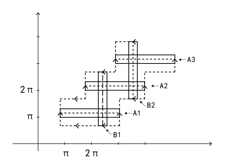
Figure 1. The flat surface $Y$

Similar to Lemma 3.2, we have:

Lemma 4.1.

The $\epsilon$-neighborhood $X_{\epsilon}$ is diffeomorphic to the manifold $Y$, and the Dehn twists $\tau_{i}$ on $X_{\epsilon}$ are conjugate to $T_{i}$ on $Y$ of the form $T_{i}(x,y)=(x+r(y-i\pi),y)$ for $i$ odd and $T_{j}(x,y)=(x,y-r(x-(j+1)\pi))$ for $j$ even.

Proof.

Since different coordinates for the plumbing map yields the same symplectic manifold, we choose a specific coordinate for the plumbing map. Similar to Section 3, we construct the plumbing maps as follows.

Suppose $p_{i}=S_{i}\cap S_{i+1}$ in $P_{\psi}(S_{1},S_{2},...,S_{m})$. For every $1\leq i\leq m$, we identify $S_{i}$ with the standard $n$-sphere $\mathbb{S}^{n}=\{x\in\mathbb{R}^{n+1}\ |\ |x|^{2}=1\}\subset\mathbb{R}^{n+1}$ through $\phi_{i}:S_{i}\to\mathbb{S}^{n}$ such that $\phi_{i}(p_{i-1})=(0,\ldots,0,1);\phi_{i}(p_{i})=(0,\ldots,0,-1)$ (for $i=1,m$ we only have the requirement for $p_{1}$ and $p_{m-1}$). On $\mathbb{S}^{n}\subset\mathbb{R}^{n+1}$ we take the local coordinates at $(0,\ldots,0,1)\in U_{+}=\{x\in\mathbb{S}^{n}\ |\ x_{n+1}>0\}$ and $(0,\ldots,0,-1)\in U_{-}=\{x\in\mathbb{S}^{n}\ |\ x_{n+1}<0\}$ respectively, given by:

$$\varphi_{\pm}:U_{\pm}\to\mathbb{R}^{2}:(x_{1},\ldots,x_{n},x_{n+1})\mapsto\frac{\arccos(\pm x_{n+1})}{\sqrt{1-x_{n+1}^{2}}}(x_{1},\ldots,x_{n}).$$

Now we take the plumbing maps to be $\psi_{i}=(T^{*}(\varphi_{-}\phi_{i+1}))^{-1}JT^{*}(\varphi_{+}\phi_{i})$. Take $\gamma_{i}=\phi_{i}(\{x\in\mathbb{S}^{n}\ |\ x_{2}=\ldots=x_{n}=0\})$ to be a great circle on $S_{i}$ given by the geodesic circle on $\mathbb{S}^{n}$. Then we see from the construction of the plumbing that $\psi_{i}(\gamma_{i+1})\subset T^{*}\gamma_{i}$ and $\psi_{i}(\gamma_{i})\subset T^{*}\gamma_{i-1}$. Thus we have $\tau_{j}(T^{*}\gamma_{i})\subset T^{*}(\gamma_{j})$ for any $1\leq j\leq m$.

On the other hand, the 2 dimensional submanifold $X_{\epsilon}$ can also be endowed with a flat structure and viewed as a open subset of a translation surface. Similar to the case of composition of two Dehn twists, we give the following local coordinates on $X$, or equivalently, we construct a 2-manifold $Y$ diffeomorphic to $X$, which can be viewed as $m$ thin bands glued together one by one, as shown in Figure 1.

The diffeomorphism from $Y$ to $X_{\epsilon}$ is given by diffeomorphisms

$$\zeta_{i}:\ A_{[\frac{i+1}{2}]}\to T^{*}\gamma_{i};\quad(x,y)\mapsto\omega_{i}(e^{\sqrt{-1}(x-\frac{i+1}{2}\pi)(-1)^{i-1}})\omega_{i+1}(e^{y\sqrt{-1}(-1)^{i-1}})p_{i}$$

for $i$ odd and

$$\zeta_{i}:\ B_{[\frac{i}{2}]}\to T^{*}\gamma_{i}(\epsilon);\quad(x,y)\mapsto\omega_{i}(e^{\sqrt{-1}(y-\frac{i+2}{2}\pi)(-1)^{i-1}})\omega_{i+1}(e^{\sqrt{-1}x(-1)^{i}})p_{i}$$

for $i$ even, where $\omega_{i}$ is the rotation on $T^{*}\gamma_{i}$ as given in equation (3.4) on the standard sphere under identification $T^{*}\phi_{i}$. By the same reasoning as in equation (3.5) in section 3, it gives a well-defined diffeomorphism from $Y$ to $X_{\epsilon}$. Similar computations as in Lemma 3.2 yeilds the conjugates $T_{i}$ of $\tau_{i}$.

∎

4.2. Hyperbolicity and positive topological entropy

In this section, we give the proof of Theorem 1.2. In fact, we shall prove the hyperbolicity of the multi-linked twist maps $T_{1}^{k_{1}}\ldots T_{m}^{k_{m}}$, which by Pesin entropy formula and the variational principle gives positive topological entropy. For a preliminary on Pesin theory, we refer readers to Appendix A. In the following we set $\mathcal{T}=T_{1}^{k_{1}}\ldots T_{m}^{k_{m}}$.

For $0\leq\delta<\epsilon<1$, we take

$$Y^{1}_{\delta}=\{(x,y)\in Y\ |\ \exists\ j\in\mathbb{N},\ s.t.\ \delta<|x-j\pi|<\epsilon-\delta;\ \delta<|y-(j-1)\pi|<\epsilon-\delta\}$$

to be the intersections of $\delta$-interior of $\cup_{i=1}^{[\frac{m+1}{2}]}A_{i}\cap B_{i}$ minus the $\delta$-neighborhood of the median lines. We also take

$$Y^{2}_{\delta}=\{(x,y)\in Y\ |\ \exists j\in\mathbb{N},\ s.t.\ \delta<|x-j\pi|<\epsilon-\delta;\ \delta<|y-j\pi|<\epsilon-\delta\}$$

to be the intersections of $\delta$-interior of $\cup_{i=1}^{[\frac{m}{2}]}B_{i}\cap A_{i+1}$ minus the $\delta$-neighborhood of the median lines as shown in Figure 2.

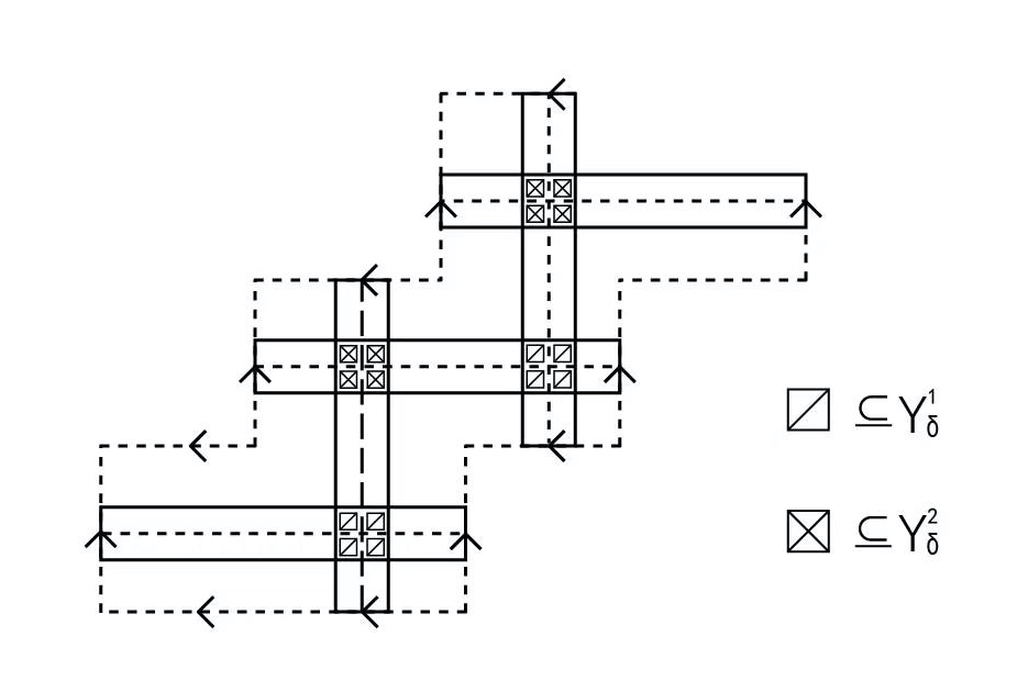
Figure 2. $Y_{\delta}^{1}$ and $Y_{\delta}^{2}$ in $Y$

We denote the set of points returning sufficiently often to $Y^{1}_{\delta}$ by

$$A_{\delta}=\{p\in Y\ |\ \liminf_{N\to\infty}\frac{1}{N}\sum_{k=1}^{N}1_{Y^{1}_{\delta}}(\mathcal{T}^{k}p)\geq\delta\},$$

and the set of points returning sufficiently often to $Y^{2}_{\delta}$ by

$$B_{\delta}=\{p\in Y\ |\ \liminf_{N\to\infty}\frac{1}{N}\sum_{k=1}^{N}1_{Y^{2}_{\delta}}(\mathcal{T}^{k}p)\geq\delta\}.$$

We first show that $\mathcal{T}$ is hyperbolic on $A_{\delta}$ and $B_{\delta}$.

Lemma 4.2.

Given $\delta>0$, there exists $c_{\delta}$ such that for any $p\in A_{\delta}\cup B_{\delta}$, the Lyapunov exponent $\chi^{+}(p)\geq c_{\delta}$.

Lemma 4.3.

Let $\mu$ be the Lebesgue probability measure on $Y$, we have $\mu(\cup_{\delta>0}(A_{\delta}\cup B_{\delta}))=1$.

We postpone the proofs to Section 4.3. With these lemmas, we prove our assertion that $\tau$ has positive topological entropy.

Proof of Theorem 1.2.

By Lemma 4.3 we have $\mu(\cup_{\delta>0}(A_{\delta}\cup B_{\delta}))=1$, thus there exists $\delta_{0}>0$ for which $\mu(A_{\delta_{0}}\cup B_{\delta_{0}})>0$. By Lemma 4.2, there exists $c>0$ such that $\chi^{+}(x)>c$ for any $x\in A_{\delta_{0}}\cup B_{\delta_{0}}$. Thus by Pesin entropy formula we have $h_{\mu}(\mathcal{T})\geq c\mu(A_{\delta_{0}}\cup B_{\delta_{0}})>0$, so by the variational principle we have

$$h_{top}(\tau)\geq h_{top}(\tau\mid X)=h_{top}(\mathcal{T})\geq h_{\mu}(\mathcal{T})>0.$$

∎

4.3. Proofs of the lemmas

In this section, we give the proofs of Lemma 4.2 and Lemma 4.3.

Proof of Lemma 4.2.

In this proof we take $\prod$ to be the ordered product read from right to left and we denote by $1_{\mathbb{N}}$ the indicator function that takes value $1$ on $\mathbb{N}$ and 0 elsewhere. For any $n\in\mathbb{N}$ and any $p\in A_{\delta}\cup B_{\delta}$, we have

$$D\mathcal{T}^{n}(p)=\prod_{i=1}^{n}\left(\begin{pmatrix}1&t_{1}^{i}\\ 0&1\end{pmatrix}\begin{pmatrix}1&0\\ t_{2}^{i}&1\end{pmatrix}...\begin{pmatrix}1&1_{\mathbb{N}}((m+1)/2)\cdot t_{m}^{i}\\ 1_{\mathbb{N}}(m/2)\cdot t_{m}^{i}&1\end{pmatrix}\right)$$

where

$$t^{i}_{j}=\left\{\begin{array}[]{l r}k_{j}r^{\prime}(y(\prod_{\ell=m}^{j+1}T_{\ell}^{k_{\ell}}\mathcal{T}^{i-1}p)-j\pi)&j\text{ odd}\\ k_{j}r^{\prime}(x(\prod_{\ell=m}^{j+1}T_{\ell}^{k_{\ell}}\mathcal{T}^{i-1}p)-(j+1)\pi)&j\text{ even}\end{array}\right..$$

Thus we have $t^{i}_{j}\geq 0$ for any $1\leq j\leq m,1\leq i\leq n$.

For $p\in A_{\delta}\cup B_{\delta}$, assume without loss of generality that $p\in A_{\delta}$, then for any $n$ sufficiently large, we have $\#\{\{\mathcal{T}^{i}(p)\ |\ 0\leq i\leq n\}\cap A_{\delta}\}\geq\delta n/2$. We number the iterations when $p$ hits $A_{\delta}$ by $\{n_{k}\}_{k\in\mathbb{N}}=\{n\in\mathbb{N}\ |\ \mathcal{T}^{n}(p)\in A_{\delta}\}$ where $n_{i}<n_{i+1}$. Then for any $k\in\mathbb{N}$, $\mathcal{T}^{n_{k}}(p)$ and $\mathcal{T}^{n_{k+1}}(p)$ are both in $A_{\delta}$. Suppose $\mathcal{T}^{n_{k}}(p)\in A_{j(n_{k})}\cap B_{j(n_{k})}$, $\mathcal{T}^{n_{k+1}}(p)\in A_{j(n_{k+1})}\cap B_{j(n_{k+1})}$ then we claim that

$$t_{2j(n_{k})}^{n_{k}}>c_{1}\text{ and }t_{2j(n_{k+1})-1}^{n_{k+1}-1}>c_{1},$$

where the constant $c_{1}>0$ is taken so that $r^{\prime}(t)>c_{1},\forall\ \delta\leq|t|\leq\epsilon-\delta$ and depends only on $r$ and $\delta$.

To prove the claim we just note that if $q=\mathcal{T}^{n_{k}}(p)$ starts from $A_{\delta}\cap A_{j(n_{k})}\cap B_{j(n_{k})}$, $T_{j}$ acts by identity on $q$ for $j>2j(n_{k})$ and so $t_{2j(n_{k})}^{n_{k}}>k_{2j(n_{k})}c_{1}$. Similarly, whenever $q=\mathcal{T}^{n_{k+1}}$ lands in $A_{\delta}\cap A_{j(n_{k+1})}\cap B_{j(n_{k+1})}$, we see that $T_{j}^{-1}(q)=q$ for $j<2j(n_{k+1})-1$ which ensures that $t_{2j(n_{k+1})-1}^{n_{k+1}-1}>k_{2j(n_{k+1})-1}c_{1}$.

Thus we showed that for $p\in A_{\delta}$, we have $\#\{1\leq i\leq n\ |\ t^{i}_{j}>c_{1}\text{ for some }j\}\geq\delta n/2$ for $n$ sufficiently large. The case $p\in B_{\delta}$ can be proved in the same way.

We next introduce a partial ordering $\leq$ on $\mathbb{R}^{2}$ given by $u=(u_{1},u_{2})\leq v=(v_{1},v_{2})$ if $u_{1}\leq v_{1},u_{2}\leq v_{2}$. We note that $T_{j}^{k_{i}}u\leq T_{j}^{k_{j}}v$ if $u\leq v$ and $T_{j}^{k_{i}}u\geq u$ if $u\geq 0$. Also, for $u\geq 0$, $t^{i}_{j}>c_{1}$, we have

$$\begin{pmatrix}1&1_{\mathbb{N}}((j+1)/2)\cdot t_{j}^{i}\\ 1_{\mathbb{N}}(j/2)\cdot t_{j}^{i}&1\end{pmatrix}u\geq\begin{pmatrix}1&1_{\mathbb{N}}((j+1)/2)\cdot c_{1}\\ 1_{\mathbb{N}}(j/2)\cdot c_{1}&1\end{pmatrix}u.$$

Thus by our claim above, for $u$ in the first quadrant, we have

$$D\mathcal{T}^{n}(p)[u]\geq\left(\begin{pmatrix}1&0\\ c_{1}&1\end{pmatrix}\begin{pmatrix}1&c_{1}\\ 0&1\end{pmatrix}\right)^{[\delta n/2]}u=\begin{pmatrix}1&c_{1}\\ c_{1}&1+c_{1}^{2}\end{pmatrix}^{[\delta n/2]}u.$$

This implies that

$$\big{\|}D\mathcal{T}^{n}(p)[u]\big{\|}\geq\left\|\begin{pmatrix}1&c_{1}\\ c_{1}&1+c_{1}^{2}\end{pmatrix}^{[\delta n/2]}u\right\|\geq c_{2}\lambda^{[\delta n/2]}\|u\|$$

for a constant $c_{2}$ depending on $u$ and $c_{1}$, where $\lambda$ is the larger eigenvalue of $\begin{pmatrix}1&c_{1}\\ c_{1}&1+c_{1}^{2}\end{pmatrix}$. Thus we have $\chi^{+}(p,u)\geq\lambda^{\delta/2}=c_{\delta}$ for any $u\geq 0$. So we get our desired result $\chi^{+}(p)\geq c_{\delta}>0$. ∎

The following lemma by Burton and Easton shows that almost every point that hits a subset of $Y$ must hit the subset sufficiently often (which can be viewed as a generalization of Poincaré recurrence theorem).

Lemma 4.4 (Burton and Easton, [8]).

Let $(F,X,\mu)$ be a measure preserving dynamical system, and $V$ be a subset of $X$. Suppose

$$P(V)=\{p\in X\ |\ \exists\ N\in\mathbb{N},\ s.t.\ F^{N}(p)\in V\}$$

is the set of points that hits $V$,

$$Z(V)=\{p\in X\ |\ \liminf_{N\to\infty}\frac{1}{N}\sum_{k=0}^{N}1_{V}(F^{N}(p))=0\}$$

is the set of points that do not hit $V$ at a positive average rate, then we have $\mu(P(V)\cap Z(V))=0$.

Proof.

By definition $Z(V)$ is an $F$-invariant set of $X$. Thus we have

$$\int_{Z(V)}1_{V}(x)d\mu(x)=\int_{Z(V)}1_{V}(F^{N}(x))d\mu(x)=$$

$$\int_{Z(V)}\liminf_{N\to\infty}\frac{1}{N}\sum_{k=0}^{N}1_{V}(F^{N}(x))d\mu(x)=0.$$

So we get $\mu(V\cap Z(V))=0$. Furthermore, we have $\mathcal{T}^{-k}(V\cap Z(V))=\mathcal{T}^{-k}(V)\cap Z(V)$ for any $k\in\mathbb{N}$. This implies that $\mu(P(V)\cap Z(V))=\mu(\cup_{k\in\mathbb{N}}(\mathcal{T}^{-k}(V)\cap Z(V)))=0$. ∎

We next show that indeed almost very point in $Y$ hits $Y^{1}_{0}\cup Y^{2}_{0}$ eventually.

Lemma 4.5.

For Lebesgue almost every point $p$ in $Y$, there exists $N\in\mathbb{N}$ such that $\mathcal{T}^{N}(p)\in Y^{1}_{0}\cup Y^{2}_{0}$.

Proof.

We notice that

$$Y^{1}_{0}\cup Y^{2}_{0}=\cup_{i\neq j}(Y_{i}\cap Y_{j})-\{(x,y)\ |\ x\in\mathbb{N}\text{ or }y\in\mathbb{N}\}.$$

First we note that the set of points ever hitting $\{(x,y)\ |\ x\in\mathbb{N}\text{ or }y\in\mathbb{N}\}$ has zero Lebesgue measure since $vol(\{(x,y)\ |\ x\in\mathbb{N}\text{ or }y\in\mathbb{N}\})=0$. Thus we only need to consider points that never hits $\cup_{i\neq j}(Y_{i}\cap Y_{j})$.

If $\mathcal{T}^{n}(p)\notin\cup_{i\neq j}(Y_{i}\cap Y_{j}),\forall n\in\mathbb{N}$, then suppose $p\in Y_{i}$, then any iteration $\mathcal{T}^{n}(p)$ is in $Y_{i}\backslash\cup_{j\neq i}Y_{j}$. $\mathcal{T}$ restricted to $Y_{i}\backslash\cup_{j\neq i}Y_{j}$ is simply $T_{i}^{k_{i}}$ which is a single Dehn twist. Thus for $\mathcal{T}^{n}(p)\in Y_{i}\backslash\cup_{j\neq i}Y_{j},\forall n$, the point $p$ has to be periodic with $|\mathcal{T}(p)-p|>\epsilon$. Thus we see that such points must lie on finitely many 1-dimensional segments, so they make up a measure zero subset of $Y$. ∎

Now we finish the proof the the lemmas.

Proof of Lemma 4.3.

We only need to prove that $\mu(\cup_{n\in\mathbb{N}}(A_{\frac{1}{n}}\cup B_{\frac{1}{n}}))=1$.

We follow the notations in Lemma 4.5. By Lemma 4.5, since $\cup_{\delta>0}Y^{i}_{\delta}=Y^{i}_{0},i=1,2$, for almost every $p\in Y$, there exists $n>0,N\in\mathbb{N}$ such that $\mathcal{T}^{N}(p)\in Y^{1}_{\frac{1}{n}}\cup Y^{2}_{\frac{1}{n}}$, i.e.

$$\mu\big{(}\cup_{n\in\mathbb{N}}(P(Y^{1}_{\frac{1}{n}}\big{)}\cup P(Y^{2}_{\frac{1}{n}})))=1.$$

By Lemma 4.4, we have $\mu(P(Y^{i}_{\delta})\cap Z(Y^{i}_{\delta}))=0,\forall\delta$ which implies

$$\mu\left(\bigcup_{m\in\mathbb{N}}\left(P(Y^{i}_{\frac{1}{n}})\bigcap\left\{p\in Y\ |\ \liminf_{N\to\infty}\frac{1}{N}\sum_{k=0}^{N}1_{Y^{i}_{\frac{1}{n}}}(F^{N}(p))>\frac{1}{m}\right\}\right)\right)=\mu(P(Y^{i}_{\frac{1}{n}})),$$

for $i=1,2.$ Now since $Y^{i}_{\frac{1}{n}}\subset Y^{i}_{\frac{1}{m}}$ for $n<m$, the last equation implies that

$$\mu\big{(}P(Y^{1}_{\frac{1}{n}})\cap(\cup_{m\in\mathbb{N}}A_{\frac{1}{m}})\big{)}=\mu(P(Y^{1}_{\frac{1}{n}})),\quad\mu(P(Y^{2}_{\frac{1}{n}})\cap(\cup_{m\in\mathbb{N}}B_{\frac{1}{m}}))=\mu(P(Y^{2}_{\frac{1}{n}}))$$

for any $n\in\mathbb{N}$. Combining this with $P(Y^{i}_{\frac{1}{n}})\subset P(Y^{i}_{\frac{1}{m}})$ for any $n<m$ and $\mu(\cup_{n\in\mathbb{N}}(P(Y^{1}_{\frac{1}{n}})\cup P(Y^{2}_{\frac{1}{n}})))=1$, we have

$$\mu\big{(}\cup_{n\in\mathbb{N}}(A_{\frac{1}{n}}\cup B_{\frac{1}{n}})\big{)} =\mu\left(\big{(}\cup_{m\in\mathbb{N}}(A_{\frac{1}{m}}\cup B_{\frac{1}{m}})\big{)}\bigcap\big{(}\cup_{n\in\mathbb{N}}(P(Y^{1}_{\frac{1}{n}})\cup P(Y^{2}_{\frac{1}{n}}))\big{)}\right)$$

$$\geq\mu\left(\cup_{n\in\mathbb{N}}\big{(}P(Y^{1}_{\frac{1}{n}})\cap(\cup_{m\in\mathbb{N}}A_{\frac{1}{m}})\big{)}\bigcup\big{(}\cup_{n\in\mathbb{N}}(P(Y^{2}_{\frac{1}{n}})\cap(\cup_{m\in\mathbb{N}}B_{\frac{1}{m}}))\big{)}\right)$$

$$=\mu\left(\cup_{n\in\mathbb{N}}\big{(}P(Y^{1}_{\frac{1}{n}})\cup P(Y^{2}_{\frac{1}{n}})\big{)}\right)=1.$$

This completes the proof. ∎

5. Rotation map and the local stable/unstable Lagrangian manifolds

As a corollary of Lemma 4.2 and Lemma 4.3, in this section, we also prove the existence of local stable/unstable Lagrangian manifolds using Pesin’s stable manifold theorem and a rotation construction. We start with the definition of rotation map that brings curves from the reduced 2-dimensional space $P_{\psi}(\gamma_{1},\ldots,\gamma_{m})$ back to Lagrangian submanifolds in $P_{\psi}(S_{1},\ldots,S_{m}).$

5.1. Rotation map on the standard sphere

First we define the rotation map on the standard sphere $\mathbb{S}^{n}$.

Definition 5.1.

Let $\gamma$ be the great circle $\{(y_{1},0,\ldots,0,y_{n+1})\}$ on $\mathbb{S}^{n}$ passing through the two point $\mathbf{n}=(0,\ldots,0,1)$ and $-\mathbf{n}=(0,\ldots,0,-1)$ called north pole and south pole respectively. Let $\mathbb{S}^{n-1}=\{(\theta,0)\in\mathbb{R}^{n}\times\mathbb{R}\ |\ |\theta|^{2}=1\}$ be the the equator of $\mathbb{S}^{n}$. We suppose that $\gamma$ has angle coordinate $\theta=(1,0,\ldots,0)\in\mathbb{S}^{n-1}$ and $\gamma_{\theta}$ is one with angle $\theta\in\mathbb{S}^{n-1}$. We associate to $\theta$ the rotation map $\mathcal{R}_{\theta}$, an element in $\mathrm{SO}(n)$ sending $T^{*}\gamma$ to $T^{*}\gamma_{\theta}$ isometrically. More precisely, let $x=(\theta,0),\theta\in\mathbb{S}^{n-1}$ be a point on the equator. We define

$$\mathcal{R}_{\theta}:\ T^{*}\gamma=\{(y_{1},0,\ldots,0,y_{n+1},\;v_{1},0,\ldots,0,v_{n+1})\in T^{*}\mathbb{S}^{n}\}\longrightarrow T^{*}\mathbb{S}^{n}$$

$$(y_{1},0,\ldots,0,y_{n+1},\;v_{1},0,\ldots,0,v_{n+1})\longmapsto(y_{n+1}\cdot\mathbf{n}+y_{1}\cdot x,\;v_{n+1}\cdot\mathbf{n}+v_{1}\cdot x).$$

Hereafter we call $\mathcal{R}_{\theta}$ the rotation map.

Note that for all points $\theta\in\mathbb{S}^{n-1}$ we have $\mathcal{R}_{\theta}(\pm\mathbf{n},\mathbf{0})=(\pm\mathbf{n},\mathbf{0})$, and if $p\notin\{(\pm\mathbf{n},\mathbf{0})\}$ in $T^{*}\gamma$ the union of images $\cup_{\theta\in\mathbb{S}^{n-1}}\mathcal{R}_{\theta}(p)$ is an embedded $(n-1)$-sphere in $T^{*}\mathbb{S}^{n}$.

Lemma 5.1.

Let $c:\ [0,1]\to T^{*}\gamma$ be an embedded curve. Then the set

(5.1) $$L_{c}=\bigcup_{\theta\in\mathbb{S}^{n-1}}\mathcal{R}_{\theta}\big{(}c([0,1])\big{)}$$

is an immersed Lagrangian submanifold $($possibly with boundary$)$ of $T^{*}\mathbb{S}^{n}$ which possibly has non-smooth points at $(\pm\mathbf{n},\mathbf{0})$.

Proof.

Let $c(t)=(y_{1}(t),0,\ldots,0,y_{n}(t),\;v_{1}(t),0,\ldots,0,v_{n}(t))$. By definition we have

$$L_{c}=\{(y_{1}(t)\theta,y_{n}(t);v_{1}(t)\theta,v_{n}(t))\ |\ t\in[0,1],\theta\in\mathbb{S}^{n-1}\subset\mathbb{R}^{n}\}.$$

Thus it is a smoothly immersed submanifold outside the south and north pole.

To verify it is lagrangian, we have $\omega|_{L_{c}}=0$ if and only if $\sum_{i=1}^{n+1}dy_{i}\wedge dv_{i}|_{L_{c}}=0$. To verify the latter, we compute

$$\sum_{i}d(y_{1}(t)\theta_{i})\wedge d(v_{1}(t)\theta_{i})+dy_{n+1}(t)\wedge dv_{n+1}(t)$$

$$=(y_{1}(t)v_{1}^{\prime}(t)-v_{1}(t)y_{1}^{\prime}(t))\sum_{i}\theta_{i}d\theta_{i}=\frac{(y_{1}(t)v_{1}^{\prime}(t)-v_{1}(t)y_{1}^{\prime}(t))}{2}d\big{(}\sum_{i}\theta_{i}^{2}\big{)}=0,$$

where in the last inequality we have used $\sum\theta_{i}^{2}=1$. Thus we see that $L_{c}$ is locally Lagrangian. ∎

Since the Dehn twist $\tau$ acts as geodesic flow along the cotangent bundle of any geodesic circle in $\mathbb{S}^{n}$, we see that it is commutative with the rotation map.

Lemma 5.2.

For the symplectic Dehn twists $\tau$ along $T^{*}\mathbb{S}^{n}$ we have

(5.2) $$\mathcal{R}_{\theta}\circ\tau|_{T^{*}\gamma}=\tau\circ\mathcal{R}_{\theta}|_{T^{*}\gamma},$$

and

(5.3) $$\tau(L_{c})=L_{\tau(c)}$$

for any smooth curve $c:\ [0,1]\to T^{*}\gamma$.

5.2. Rotation map on the plumbing space

Let $\gamma_{i}\subset S_{i}$, $i=1,\ldots,m$ be a geodesic circle which contains a plumbing point and its antipodal point (denoted by $p_{i}$ and $-p_{i}$) of $S_{i}$ as given in Section 4. Then for each $i=1,\ldots,m-1$, the plumbing map $\psi_{i}$ sends an open subset of $p_{i}$ in $T^{*}\gamma_{i}$ onto that of $-p_{i+1}$ in $T^{*}\gamma_{i+1}$. In other words, the restriction of $\psi_{i}$ to $T^{*}\gamma_{i}$ gives rise to the plumbing map from $T^{*}\gamma_{i}$ to $T^{*}\gamma_{i+1}$, from which we get a plumbing space denoted by $P_{\psi}(\gamma_{1},\gamma_{2},\ldots,\gamma_{m})$.

We identify each $S_{i}$ with $\mathbb{S}^{n}$ through a map $\phi_{i}:\ S_{i}\to\mathbb{S}^{n}$ such that the image of the great circle $\gamma$ is exactly $\gamma_{i}$. Then for each $\theta\in\mathbb{S}^{n-1}$, the rotation maps defined above give rise to a symplectic map $\mathcal{R}_{\theta}^{i}:\ T^{*}\gamma_{i}\to T^{*}S_{i}$ by

$$\mathcal{R}_{\theta}^{i}=(T^{*}\phi_{i})^{-1}\circ\mathcal{R}_{\theta}\circ T^{*}\phi_{i}|_{T^{*}\gamma_{i}}$$

which we call the rotation map on $S_{i}$.

To extend the Lagrangian submanifolds $L_{c}^{i}$ from a single sphere to the full space $P_{\psi}(S_{1},S_{2},\ldots,S_{m})$, we need to know the effect of the rotation maps $\mathcal{R}_{\theta}^{i}$ under the local identification maps $\psi_{i}:\ T^{*}U_{i}^{+}\to T^{*}U_{i+1}^{-}$, where the open subsets $U_{i}^{\pm}\subset S_{i}$ are the preimages of the open subsets

$$U_{\pm}=\{x=(x_{1},x_{2},...,x_{n+1})\in\mathbb{R}^{n+1}\ |\ |x|^{2}=1,\ \pm x_{n+1}>0\}\subset\mathbb{S}^{n}$$

under the map $\phi_{i}:\ S_{i}\to\mathbb{S}^{n}$.

Lemma 5.3.

Let $P_{\psi}(S_{1},\ldots,S_{n})$ be the plumbing space with chosen local identification maps $\psi_{i}$ (as given in Lemma 3.2 and Lemma 4.1). Then we get that for any $\theta\in\mathbb{S}^{n-1}$ and any geodesic circle $\gamma$ of $S_{i}$ containing the plumbing point $p$ of $S_{i}$ with $S_{i+1}$, we have

(5.4) $$\mathcal{R}_{\theta}^{i+1}\circ\psi_{i}=\psi_{i}\circ\mathcal{R}_{\theta}^{i}\quad\hbox{on}\;T^{*}\gamma\cap U_{i}^{+},$$

where $U_{i}^{+}$ is the plumbing region of $p_{i}$ in $T^{*}S_{i}$.

Proof.

Note that the plumbing map $\psi_{i}$ is given by $(d\varphi_{i+1}^{-})^{-1}Jd\varphi_{i}^{+}$ where $\varphi_{j}^{\pm}=\phi_{j}|_{U_{j}^{\pm}}\varphi_{\pm}:U_{j}^{\pm}\to\mathbb{R}^{n}$ with

$$\varphi_{\pm}:\ (x_{1},\ldots,x_{n+1})\mapsto\frac{\arccos(\pm x_{n+1})}{\sqrt{1-x_{n+1}^{2}}}(x_{1},\ldots,x_{n})$$

as in Lemma 3.2. Then by the definition of $\mathcal{R}_{\theta}$ we calculate that the conjugation of $\mathcal{R}^{j}_{\theta}$ via $d\varphi_{j}^{\pm}$ acting on $(d\varphi^{\pm}_{j})^{-1}(T^{*}\gamma_{j})\subset T^{*}\mathbb{R}^{n}$ is simply

$$d\varphi_{j}^{\pm}\mathcal{R}^{j}_{\theta}(d\varphi_{j}^{\pm})^{-1}=d\varphi_{\pm}\mathcal{R}_{\theta}d\varphi_{\pm}^{-1}:\ (t,0,\ldots,0;s,0,\ldots,0)\mapsto(t\theta,s\theta)\in T^{*}\mathbb{R}^{n}$$

for any $j$.

Therefore, the rotation map rotates both the base coordinates $x=(t,0,\ldots,0)$ and the fiber coordinate $v=(s,0,\ldots,0)$ to the direction of $\theta$ while the plumbing map from $S_{i}$ to $S_{i+1}$ switches the roles of base and fiber via the complex map $J$. Thus we see that they are commutative. ∎

Since we have $\mathcal{R}_{(-1,0,\ldots,0)}(T^{*}\gamma)=T^{*}\gamma$, i.e. $\mathcal{R}_{(-1,0,\ldots,0)}$ acts as a reflection on $T^{*}\gamma$, by Lemma 5.3 one can define a reflection map

(5.5) $$\begin{split}\bar{\mathcal{R}}:\ P_{\psi}(\gamma_{1},\gamma_{2},\ldots,\gamma_{m})\longrightarrow P_{\psi}(\gamma_{1},\gamma_{2},\ldots,\gamma_{m})\\ \bar{\mathcal{R}}(z)=\mathcal{R}_{(-1,0,\ldots,0)}^{i}(z)\quad\hbox{if $z\in T^{*}\gamma_{i}$}.\end{split}$$

Definition 5.2.

We call a smooth embedded curve $c\subset P_{\psi}(\gamma_{1},\gamma_{2},\ldots,\gamma_{m})$ admissible if $\bar{\mathcal{R}}(c)=c$. The set of admissible curves in $P_{\psi}(\gamma_{1},\gamma_{2},\ldots,\gamma_{m})$ is denoted by $\mathcal{C}_{ad}$.

Lemma 5.4.

Let $c$ be a smooth embedded admissible curve satisfying

$$c([0,1])\in P_{\psi}(\gamma_{1},\gamma_{2},\ldots,\gamma_{m}).$$

We denote by $L_{c}=\cup_{i=1}^{m}\cup_{\theta\in\mathbb{S}^{n}}\mathcal{R}_{\theta}^{i}(c)$ the image of $c$ under rotations, then $L_{c}$ is a smoothly embedded Lagrangian submanifold in $P_{\psi}(S_{1},\ldots,S_{m})$.

Proof.

By Lemma 5.1 and Lemma 5.3, $L_{c}$ is an immersed Lagrangian submanifold. Furthermore, the conditions that $c$ is admissible ensures that it does not have any self-intersection. Therefore, it is a smoothly embedded Lagrangian submanifold. ∎

Now we are ready to prove Theorem 1.3.

Proof of Theorem 1.3.

The group $\mathrm{SO}(n)$ acts on the plumbing space via its standard action on the sphere $\mathbb{S}^{n-1}$, more precisely, it is given by $\mathrm{SO}(n)\times P_{\psi}(S_{1},\ldots,S_{n})\to P_{\psi}(S_{1},\ldots,S_{n}):(g,p)\mapsto\mathcal{R}_{g(1,0,\ldots,0)}p$. We take $N$ to be the $\epsilon-$neighbourhood of $\cup S_{i}$ in the plumbing space.

By Theorem 3.4, we see from Pesin’s stable manifold theorem (see Theorem A.4) that $X_{\epsilon}$ admits stable and unstable curves $W^{s}(p)$ and $W^{u}(p)$ for almost every $p\in X_{\epsilon}$. Let $\Lambda$ be the set of points $p\in X_{\epsilon}$ that is hyperbolic under $\tau$. Since the stable curves are given by the Dehn twists which is commutative with the rotation map $\mathcal{R}_{\theta}$, we see that $\Lambda$ is invariant under the reflection map $\bar{\mathcal{R}}$ and the family of stable curves $W^{s}(p)$ is admissible under $\bar{\mathcal{R}}$, i.e. $\{W^{s}(p)\ |\ p\in\Lambda\}=\{\bar{\mathcal{R}}(W^{s}(p))\ |\ p\in\Lambda\}$. Thus by Lemma 5.4 we define a family of invariant Lagrangian submanifolds $\mathcal{F}^{s}=\{L_{W^{s}(p)}\ |\ p\in\Lambda\}$. Similarly, the family of unstable curves $W^{u}(p)$ in $X_{\epsilon}$ given by the inverse map also gives us a family of invariant Lagrangian submanifolds $\mathcal{F}^{u}$. ∎

6. Growth of Floer cohomology groups

In this section, we explore the symplectic aspect of the composite Dehn twists. As we have explained in the introduction, we are interested in the growth of Floer cohomology group. For a brief introduction to Lagrangian Floer theory, we refer readers to Appendix B.

In order to estimate the growth of Floer homology group, we shall employ a result due to Khovanov and Seidel [22].

Let $(M,\omega)$ be an exact symplectic manifold with $\omega=d\lambda$ which is equal to a symplectization near infinity. We assume in addition that $M$ admits an involution, i.e., $\iota:M\to M$ with $\iota\circ\iota=Id$ and $\iota^{*}\omega=\omega$ and $\iota^{*}\lambda=\lambda$. Clearly, the fixed point set $M^{\iota}$ is a symplectic submanifold of $M$. Moreover, when $L$ is a Lagrangian submanifold of $M$, its fixed part $L^{\iota}=L\cap M^{\iota}$ is again a Lagrangian submanifold of $M^{\iota}$.

Theorem 6.1 (Khovanov and Seidel [22, Proposition 5.15]).

Let $(S_{1},S_{2})$ be a pair of closed $\lambda$-exact Lagrangian submanifolds of $(M,\omega)$ with $\iota(S_{i})=S_{i},i=1,2$. Suppose that

• the intersection $C=S_{1}\cap S_{2}$ is clean, and there is an $\iota$-invariant Morse function $f$ on $C$ such that its critical points are precisely the points of $C^{\iota}=C\cap M^{\iota}$;

• there is no continuous map $u:\ [0,1]\times[0,1]\to M^{\iota}$ such that $u(0,t)=x$ and $u(1,t)=y$ for all $t$, and $u(s,0)\in S_{1}$ and $u(s,1)\in S_{2}$ for all $s$, where $x$ and $y$ are two different points of $S_{1}\cap S_{2}$.

Then $\mathrm{rank}\;\mathrm{HF}(S_{1},S_{2})=\mathrm{rank}\;H^{*}(C,\mathbb{Z}/2)=|C^{\iota}|$.

The proof of this theorem is based on equivariant transversality and a symmetry argument, for which we refer readers to [22] for details. It is important to note that the involution plays the role of reducing the dimension of the symplectic manifold and Lagrangian submanifold for the purpose of calculating the Floer cohomology group, similar to what we did in the last section when proving positive topological entropy.

In the following, we consider an explicit involution on the plumbing space $P_{\psi}(S_{1},S_{2},\ldots,S_{m})$, which will be useful to compute Lagrangian Floer cohomology.

To do this, we first consider a canonical involution on the cotangent bundle of the standard $n$-sphere. As before, we write

$$T^{*}\mathbb{S}^{n}=\big{\{}(x,v)\in\mathbb{R}^{n+1}\times\mathbb{R}^{n+1}\ |\ |x|=1,\;\langle x,v\rangle=0\big{\}}.$$

Set $\mathbf{x}=(x_{2},\ldots,x_{n})$ and $\mathbf{v}=(v_{2},\ldots,v_{n})$. We can define a symplectic involution map on $T^{*}\mathbb{S}^{n}$ by

$$\iota_{0}(x_{1},\mathbf{x},x_{n+1},v_{1},\mathbf{v},v_{n+1})=(x_{1},-\mathbf{x},x_{n+1},v_{1},-\mathbf{v},v_{n+1}).$$

Then the fixed point set of $\iota_{0}$ is precisely the cotangent bundle of a great circle $\gamma\in\mathbb{S}^{n}$

(6.1) $$\big{(}T^{*}\mathbb{S}^{n}\big{)}^{\iota_{0}}=T^{*}\gamma=\big{\{}(x_{1},\mathbf{0},x_{n+1},v_{1},\mathbf{0},v_{n+1})\in T^{*}\mathbb{S}^{n}\big{\}}.$$

Using the involution $\iota_{0}$ we can now define an involution on $P_{\psi}(S_{1},S_{2},\ldots,S_{m})$ as follows. For each sphere $S_{i}$ we pick the geodesic circle $\gamma_{i}$, which contains every plumbing point of $S_{i}$ and a symplectomorphism $\psi_{i}:\ T^{*}S_{i}\to T^{*}\mathbb{S}^{n}$ such that $\psi_{i}$ maps the zero section $S_{i}$ of $T^{*}S_{i}$ to $\mathbb{S}^{n}$ of $T^{*}\mathbb{S}^{n}$, and $\gamma_{i}$ to $\gamma$. Then we define the involution $\iota_{\gamma_{i}}$ on $T^{*}S_{i}$ by $\iota_{\gamma_{i}}=(\psi_{i})^{-1}\circ\iota_{0}\circ\psi_{i}$.

Furthermore, by the definition of $P_{\psi}(S_{1},S_{2},\ldots,S_{m})$ we can assume that $\iota_{\gamma_{i}}(p)=\iota_{\gamma_{i+1}}(p)$ for all points $p\in T^{*}S_{i}\cap T^{*}S_{i+1}$, $i=1,\ldots,m-1$. Then the involution on $P_{\psi}(S_{1},S_{2},\ldots,S_{m})$ is defined by $\iota(p)=\iota_{\gamma_{i}}(p)\quad\hbox{if}\quad p\in T^{*}S_{i}.$

By (6.1), for each sphere $S_{i}$ we have

(6.2) $$\big{(}T^{*}S_{i}\big{)}^{\iota}=T^{*}\gamma_{i},$$

which implies that the fixed point set of $\iota$ is symplectomorphic to the plumbing space $P_{\psi}(\gamma_{1},\gamma_{2},\ldots,\gamma_{m})$. Also, each zero section $S_{i}$ of $P_{\psi}(S_{1},S_{2},\ldots,S_{m})$ is invariant under the map $\iota$. Moreover, a direct calculation shows that $\iota$ and the symplectic Dehn twist $\tau_{i}$ along $S_{i}$ have the following relations:

(6.3) $$\iota\circ\tau_{i}=\tau_{i}\circ\iota,\quad i=1,\ldots,m.$$

Furthermore, we note that the involution and the rotation map on $\mathbb{S}^{n}$ satisfy

$$\iota\circ\mathcal{R}_{\theta}=\mathcal{R}_{\theta}\circ\iota$$

which gives us the following lemma.

Lemma 6.2.

Let $\gamma_{i}$ be circles chosen as above and $c$ be an embedded curve in $T^{*}\gamma_{i}$. Then Lagrangian submanifold $L_{c}$ is invariant under the involution $\iota$, that is,

(6.4) $$\iota(L_{c})=L_{c}.$$

6.1. Proof of Theorem 1.4

In this section, we give the proof of Theorem 1.4. In order to apply Theorem 6.1, we need to verify the assumptions (C1) and (C2).

Lemma 6.3.

If $\gamma_{1}$ and $\tau^{n}(\gamma_{2})$ intersect transversely, then $S_{1}$ and $\tau^{n}(S_{2})$ satisfy condition $(C1)$ of Theorem 6.1.

We shall give the proof in Section 7.2. But in general the condition (C2) of this theorem does not hold. To solve this problem, we perturb $\tau^{n}(S_{2})^{\iota}$ so that the intersections of $(S_{1})^{\iota}$ and $\tau^{n}(S_{2})^{\iota}$ become minimal. We use the following concept which can be found in the book [12].

Definition 6.1 (Geometric intersection number).

Let $\alpha$ and $\beta$ be two free homotopy classes of simple closed curves in a surface $S$. We call the minimal number of intersection points between a representative curve $a$ in the class $\alpha$ and a representative curve $b$ in the class $\beta$ the geometric intersection number between $\alpha$ and $\beta$, which we denote by $i(\alpha,\beta)$.

Lemma 6.4.

If $\gamma_{1}$ and $\tau^{n}(\gamma_{2})$ are not isotopic, we have the following equality

(6.5) $$\mathrm{rank}\;\mathrm{HF}\big{(}S_{1},\tau^{n}(S_{2})\big{)}=i\big{(}[\gamma_{1}],[\tau^{n}(\gamma_{2})]\big{)}.$$

We postpone the proof of the lemma to the next section and complete the proof of Theorem 1.4.

Proof of Theorem 1.4.

Since symplectic Dehn twists $\tau_{1}$ and $\tau_{2}$ are supported in a compact neighborhood of the zero section of $P_{\psi}(S_{1},S_{2})$, as in Section 3 we identify the action of $\tau=\tau^{k}_{2}\tau^{\ell}_{1}$ on an invariant submanifold $X_{\epsilon}\subseteq P_{\psi}(\gamma_{1},\gamma_{2})$ with the action of $\mathcal{T}=T_{2}^{k}T_{1}^{\ell}$ on an open subset $Y$ of $2$-torus $\mathbb{T}^{2}$. And the curves $\gamma_{1}$ and $\gamma_{2}$ are identified with $\beta_{1}=\{(s,0)\in\mathbb{T}^{2}\}$ and $\beta_{2}=\{(0,t)\in\mathbb{T}^{2}\}$ respectively. Then we get

(6.6) $$i\big{(}[\gamma_{1}],[\tau^{n}(\gamma_{2})]\big{)}=i_{Y}\big{(}[\beta_{1}],[\mathcal{T}^{n}(\beta_{2})]\big{)}\geq i_{\mathbb{T}^{2}}\big{(}[\beta_{1}],[\mathcal{T}^{n}(\beta_{2})]\big{)}.$$

So by (6.5) to prove Theorem 1.4 we need to estimate the growth rate of the geometric intersection number $i_{\mathbb{T}^{2}}\big{(}[\beta_{1}],[\mathcal{T}^{n}(\beta_{2})]$ as $n\to\infty$.

It is well-known that the mapping class group $\hbox{Mod}(\mathbb{T}^{2})$ of $\mathbb{T}^{2}$ is $\mathrm{PSL}_{2}\mathbb{Z}$, and the nontrivial free homotopy classes of oriented simple closed curves in $\mathbb{T}^{2}$ are in bijective correspondence with primitive elements of $\mathbb{Z}^{2}$. Moreover, the geometric intersection number of two such homotopy classes $(a,b),(c,d)\in\mathbb{Z}^{2}$ can be computed as

(6.7) $$i_{\mathbb{T}^{2}}\big{(}(a,b),(c,d)\big{)}=|ad-bc|,$$

see, for instance, [12, Section 1.2.3]. From Lemma 3.2 we see that $T_{1}$ and $T_{2}$, representing an element of $\hbox{Mod}(\mathbb{T}^{2})$, have the forms $\left(\begin{array}[]{cc}1&1\\ 0&1\end{array}\right)\quad\hbox{and}\quad\left(\begin{array}[]{cc}1&0\\ -1&1\end{array}\right)$ respectively. For $k,\ell\in\mathbb{N}$, the mapping class of $\mathcal{T}=T_{2}^{k}T_{1}^{\ell}$ is given by $\left(\begin{array}[]{cc}1-k\ell&l\\ -k&1\end{array}\right)$. If $k\ell\neq 0,1,2,3,4$, then this matrix has a similar diagonalizable matrix $\left(\begin{array}[]{cc}\lambda&0\\ 0&\lambda^{-1}\end{array}\right)$ with the eigenvalue $|\lambda|>1$. In this case, using (6.7) an easy calculation shows that

(6.8) $$\lim_{n\to\infty}\sqrt[n]{i_{\mathbb{T}^{2}}\big{(}[\beta_{1}],[\mathcal{T}^{n}(\beta_{2})]\big{)}}=|\lambda|.$$

Clearly, for sufficiently large $n$, $\beta_{1}$ and $\mathcal{T}^{n}(\beta_{2})$ are not isotopic, and so for $\gamma_{1}$ and $\tau^{n}(\gamma_{2})$. Then it follows from (6.5), (6.6) and (6.8) that

$$\Gamma(\tau,S_{1},S_{2})=\liminf_{n\to\infty}\frac{\log\mathrm{rank}\;\mathrm{HF}(S_{1},\phi^{n}(S_{2}))}{n}\geq\log|\lambda|>0.$$

The proof of the case that $\tau=\tau_{1}^{k}\tau_{2}^{\ell}$ is similar, and so we omit it here. This completes the proof of statement (1).

Proof of statement (2). When $k\ell=0,1,2,3,4$, then we have that the matrix $\left(\begin{array}[]{cc}1-k\ell&l\\ -k&1\end{array}\right)$ is a periodic or reducible mapping class, then the growth of Floer cohomology group is zero.

Proof of statement (3). The claim that $\Gamma(\tau_{i}^{2},S_{j},S_{j})=0$, $i,j\in\{1,2\}$ with $i\neq j$ follows from the following well-known result immediately.

Lemma 6.5 ([18, Proposition 4.7]).

Let $(M^{2n},\omega)$ be a connected Liouville domain with $n$ even and $2c_{1}(M,\omega)=0$. If $M$ contains an $A_{2}^{n}$-configuration of Lagrangian spheres $(S_{1},S_{2})$, then for any $k\in\mathbb{N}\cup\{0\}$, it holds that

$$\mathrm{rank}\;\mathrm{HF}(S_{i},\tau_{j}^{2k}(S_{i}))=2k,\;i,j\in\{1,2\}\;\hbox{with}\;i\neq j.$$

The proof of this lemma is essentially due to Seidel’s long exact sequence for Floer cohomology of Dehn twists [29, Theorem 1], see also Keating [20, Section 6]. The plumbing space $P(S_{1},S_{2})$ is a symplectization of Liouville domain with contact-type boundary which satisfies the conditions of the above lemma, see, for instance, [1, Section 2.3].

∎

6.2. Proof of Theorem 1.5

The proof of Theorem 1.5 is similar to that of Theorem 1.4. Let $P_{\psi}(S_{1},S_{2},\ldots,S_{m})$ and $P_{\psi}(\gamma_{1},\gamma_{2},\ldots,\gamma_{m})$ be the plumbing spaces as given in Section 5.2. We need to verify the conditions (C1) and (C2) of Theorem 6.1. Similar to Lemma 6.4, we have the following lemma.

Lemma 6.6.

We have the equality

(6.9) $$\mathrm{rank}\;\mathrm{HF}\big{(}S_{i},\tau^{n}(S_{j})\big{)}=i\big{(}[\gamma_{i}],[\tau^{n}(\gamma_{j})]\big{)}.$$

To complete the proof of Theorem 1.5 the remaining task is to show that $i([\gamma_{i}],[\tau^{n}(\gamma_{j})])$ grows exponentially as $n\to\infty$. To do this, we need some knowledge from the subject of mapping class groups, which we will present below.

By definition, a collection of isotopy classes of simple closed curves in a closed surface $S$ with genus $g\geq 2$ fills $S$ if the complement in $S$ of the representatives in the surface is a collection of topological disks. (Equivalently, any simple closed curve in $S$ has positive geometric intersection with some isotopy class in the collection). A multicurve in $S$ is the union of a finite collection of disjoint simple closed curves in $S$.

Theorem 6.7 (Penner [25, Theorem 3.1]).

Let $A=\{c_{1},\ldots,c_{n}\}$ and $B=\{d_{1},\ldots,d_{m}\}$ be two multicurves in a surface $S$ which fill $S$. Then any composition of positive powers of Dehn twists $T_{c_{i}}$ along $c_{i}$ and negative powers of Dehn twists $T_{d_{j}}$ along $d_{j}$ is pseudo-Anosov, where each $c_{i}$ and $d_{j}$ appears at least once.

Theorem 6.8 ([14]).

Let $f$ be a pseudo-Anosov mapping class of a closed surface $S$ of genus $g\geq 2$ with stretch factor $\lambda>1$. Then for any two isotopy classes of curves $\alpha$ and $\beta$ we have $\lim_{n\to\infty}\sqrt[n]{i\big{(}\alpha,f^{n}(\beta))}=\lambda.$

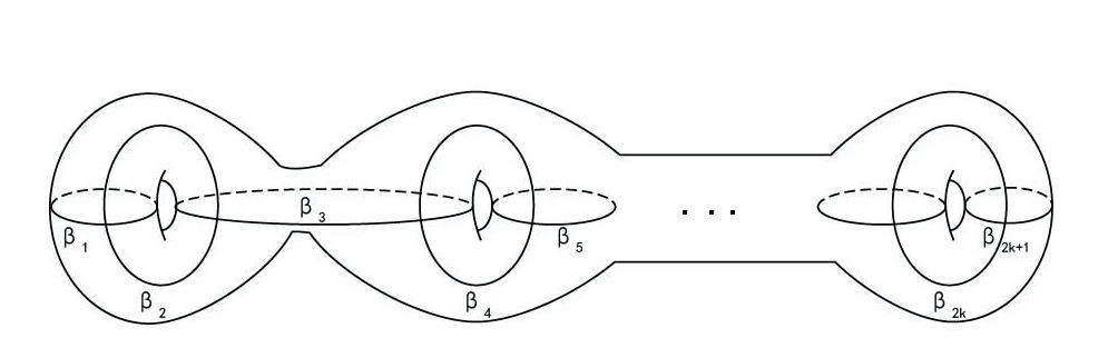
Figure 3. Curves filling a surface of genus $g=k$

Proof of Theorem 1.5.

Now we are in position to finish the proof. Notice that each symplectic Dehn twist $\tau_{i}$ is supported in a compact neighborhood of the zero section of $S_{i}$. One can identify the action of $\tau=\tau_{1}^{k_{1}}\tau_{2}^{k_{2}}\cdots\tau_{m}^{k_{m}}$ on an invariant submanifold $X_{\epsilon}\subseteq P_{\psi}(\gamma_{1},\gamma_{2},\ldots,\gamma_{m})$ with the action of $\mathcal{T}=T_{1}^{k_{1}}T_{2}^{k_{2}}\cdots T_{m}^{k_{m}}$ on an open subset $Y$ of a closed surface of genus $g$. More precisely, for $m=2k,2k+1$ one can embed curves $\gamma_{1},\ldots,\gamma_{m}$ into a surface $S$ of genus $g=k$ with images $\beta_{1},\ldots,\beta_{m}$ as illustrated in Picture 3 (when $m=2k$, we do not need $\beta_{2k+1}$), and $X_{\epsilon}$ is identified with the union $Y$ of open neighborhoods of simple closed curves $\beta_{1},\ldots,\beta_{m}$ in $S$, and each $\tau_{i}$ corresponds to the Dehn twist $T_{i}$ along $\beta_{i}$. So we have

(6.10) $$i\big{(}[\gamma_{i}],[\tau^{n}(\gamma_{j})]\big{)}=i_{Y}\big{(}[\beta_{i}],[\mathcal{T}^{n}(\beta_{j})]\big{)}\geq i_{S}\big{(}[\beta_{i}],[\mathcal{T}^{n}(\beta_{j})]\big{)}.$$

Notice that by our construction the collection of curves $\beta_{1},\ldots,\beta_{m}$ fills $S$, and that $\beta_{i}$ and $\beta_{i+2}$, $i=1,\ldots,m-2$ are disjoint. By Theorem 6.7, if either $k_{i}>0$ for $i$ odd and $k_{i}<0$ for $k$ even, or $k_{i}>0$ for $i$ even and $k_{i}<0$ for $k$ odd, $\mathcal{T}$ is pseudo-Anosov. Then by Theorem 6.8 we have $\lim_{n\to\infty}\sqrt[n]{i_{S}\big{(}[\beta_{i}],[\mathcal{T}^{n}(\beta_{j})]\big{)}}=\lambda.$ This, together with (6.9) and (6.10), implies the desired result.

∎

7. Floer cohomology groups and intersection numbers

In this section, we relate the Floer cohomology groups to the geometric intersection numbers in the reduced space $P_{\psi}(S_{1},\ldots,S_{n})$ and give the proof of Lemma 6.4.

7.1. Rotation maps and Lagrangian isotopies

The next lemma is important for constructing Lagrangian isotopies through isotopic curves in $W:=P_{\psi}(\gamma_{1},\gamma_{2},\ldots,\gamma_{m})$. Denote $\Sigma_{\psi}$ the set consisting of plumbing points and their antipodal points in $W$. Note that if $c\in\mathcal{C}_{ad}$ is an admissible curve containing exactly two points of $\Sigma_{\psi}$ then $L_{c}$ is a Lagrangian sphere in $P_{\psi}(S_{1},S_{2},\ldots,S_{m})$. Let $\hbox{Diff}_{c}(W,\Sigma_{\psi})$ be the group of compactly supported diffeomorphisms $f:W\to W$ with $f(\Sigma_{\psi})=\Sigma_{\psi}$.

Definition 7.1.

Two curves $\gamma_{0},\gamma_{1}\in\mathcal{C}_{ad}$ are called isotopic if there is an isotopy $(f_{s})_{0\leq s\leq 1}$ in $\hbox{Diff}_{c}(W,\Sigma_{\psi})$ such that $\gamma_{s}=f_{s}(\gamma_{0})$ is a family of admissible curves connecting $\gamma_{0}$ to $\gamma_{1}$.

Definition 7.2.

A Lagrangian isotopy on a symplectic manifold $(M,\omega)$ is a smooth family of Lagrangian embedding $\Phi:L\times[0,1]\to M$. Since $\Phi^{*}\omega$ vanishes on the fibers $L\times\{\hbox{point}\}$, $\Phi^{*}\omega=\theta_{s}\wedge ds$. We call a Lagrangian isotopy $\Phi$ exact if $\theta_{s}\in\Lambda^{1}(L)$ is exact for all $s$.

The following lemma follows immediately from Lemma 5.1.

Lemma 7.1.

If $c_{1},c_{2}\in\mathcal{C}_{ad}$ are isotopic in $P_{\psi}(\gamma_{1},\gamma_{2},\ldots,\gamma_{m})$, then $L_{c_{1}}$ and $L_{c_{2}}$ are Lagrangian isotopic.

For every $c\in\mathcal{C}_{ad}$ we define an embedded Lagrangian submanifold in $P_{\psi}(S_{1},S_{2},\ldots,S_{m})$ by

$$L_{c}=L^{1}_{c_{1}}\cup_{\psi_{1}}L^{2}_{c_{2}}\cup_{\psi_{2}}\cdots\cup_{\psi_{m-1}}L^{m}_{c_{m}},$$

where each curve $c_{i}$ is the part of $c$ lying in $T^{*}\gamma_{i}$ and each $L^{i}_{c_{i}}$ denotes the Lagrangian submanifold in $T^{*}S_{i}$ as defined in Lemma 5.1. We say that $L_{c}$ is generated by $c$. By (6.4), we know that $L_{c}$ is invariant under the involution $\iota$ associated to the circles $\gamma_{1},\gamma_{2},\ldots,\gamma_{m}$, i.e.,

(7.1) $$\iota(L_{c})=L_{c}.$$

7.2. Rotation maps and Dehn twists

Set $M=P_{\psi}(S_{1},S_{2})$ and $\tau=\tau^{k}_{2}\tau^{\ell}_{1}$. As before, we identify two open neighborhoods $U_{1}$ and $U_{2}$ of the plumbing point $p$ in $T^{*}S_{1}$ and $T^{*}S_{2}$ by a symplectomorphism $\psi$. Pick a geodesic circle $\gamma_{1}$ of $S_{1}$ containing $p$, and let $\gamma_{2}$ be the unique geodesic circle of $S_{2}$ passing through $p$ such that two open subsets of $T^{*}\gamma_{1}$ and $T^{*}\gamma_{2}$ are identified near $p$ under the map $\psi$. Let $\mathcal{R}_{\theta}^{i}:T^{*}\gamma_{i}\to M,i=1,2$ be the rotation maps associated to $S_{i}$ as described in Section 5.2.

Lemma 7.2.

Let $c_{1}\subseteq T^{*}\gamma_{1}$ and $c_{2}\subseteq T^{*}\gamma_{2}$ be two smooth curves. Then for any $k\in\mathbb{Z}$ and any $\theta\in\mathbb{S}^{n-1}$ we have

(7.2) $$\begin{split}\tau_{1}^{k}\big{(}\mathcal{R}_{\theta}^{2}(c_{2})\big{)}=\mathcal{R}_{\theta}^{2}\big{(}\tau_{1}^{k}(c_{2})\cap T^{*}\gamma_{2}\big{)}\cup_{\psi}\mathcal{R}_{\theta}^{1}\big{(}\tau_{1}^{k}(c_{2})\cap T^{*}\gamma_{1}\big{)},\\ \tau_{2}^{k}\big{(}\mathcal{R}_{\theta}^{1}(c_{1})\big{)}=\mathcal{R}_{\theta}^{1}\big{(}\tau_{2}^{k}(c_{1})\cap T^{*}\gamma_{1}\big{)}\cup_{\psi}\mathcal{R}_{\theta}^{2}\big{(}\tau_{2}^{k}(c_{1})\cap T^{*}\gamma_{2}\big{)}.\end{split}$$

Proof.

(7.2) follows from (5.2) and (5.4) and the fact that every symplectic Dehn twist along a sphere preserves all cotangent bundles of geodesic circles of this sphere. We only prove the former. Let $c\subset T^{*}\gamma_{2}$ be a smooth curve. Then we have

$$\tau_{1}\big{(}\mathcal{R}_{\theta}^{2}(c)\big{)} = \tau_{1}\big{(}\mathcal{R}_{\theta}^{2}(c)\cap\mathcal{R}_{\theta}^{1}(T^{*}\gamma_{1})\big{)}\cup\tau_{1}\big{(}\mathcal{R}_{\theta}^{2}(c)\setminus\mathcal{R}_{\theta}^{1}(T^{*}\gamma_{1})\big{)}$$

$$= \tau_{1}\big{(}\mathcal{R}_{\theta}^{1}(c\cap T^{*}\gamma_{1})\big{)}\cup\big{(}\mathcal{R}_{\theta}^{2}(c)\setminus\mathcal{R}_{\theta}^{1}(T^{*}\gamma_{1})\big{)}$$

$$= \mathcal{R}_{\theta}^{1}\big{(}\tau_{1}(c\cap T^{*}\gamma_{1})\big{)}\cup\big{(}\mathcal{R}_{\theta}^{2}(c\setminus T^{*}\gamma_{1})\big{)}$$

$$= \mathcal{R}_{\theta}^{2}\big{(}\tau_{1}(c\cap T^{*}\gamma_{1})\cap T^{*}\gamma_{2}\big{)}\cup\mathcal{R}_{\theta}^{1}\big{(}\tau_{1}(c\cap T^{*}\gamma_{1})\setminus T^{*}\gamma_{2}\big{)}\cup\big{(}\mathcal{R}_{\theta}^{2}\tau_{1}(c\setminus T^{*}\gamma_{1})\big{)}$$

$$= \mathcal{R}_{\theta}^{2}\big{(}\tau_{1}(c)\cap T^{*}\gamma_{2}\big{)}\cup\mathcal{R}_{\theta}^{1}\big{(}\tau_{1}(c)\setminus T^{*}\gamma_{2}\big{)}$$

$$= \mathcal{R}_{\theta}^{2}\big{(}\tau_{1}(c)\cap T^{*}\gamma_{2}\big{)}\cup_{\psi}\mathcal{R}_{\theta}^{1}\big{(}\tau_{1}(c)\cap T^{*}\gamma_{1}\big{)}.$$

∎

Now we are ready to give the proof of Lemma 6.3.

Proof of Lemma 6.3.

Since $S_{i}=\cup_{\theta\in\mathbb{S}^{n-1}}\mathcal{R}_{\theta}^{i}(\gamma_{i}),i=1,2$, we have

(7.3) $$S_{1}\cap\tau^{n}(S_{2}) = \bigcup\limits_{\theta\in\mathbb{S}^{n-1}}\big{(}\mathcal{R}_{\theta}^{1}(\gamma_{1})\cap\tau^{n}(S_{2})\big{)}=\bigcup\limits_{\theta\in\mathbb{S}^{n-1}}\bigcup\limits_{\theta^{\prime}\in\mathbb{S}^{n-1}}\big{(}\mathcal{R}_{\theta}^{1}(\gamma_{1})\cap\tau^{n}(\mathcal{R}_{\theta^{\prime}}^{2}(\gamma_{2}))\big{)}$$

$$= \bigcup\limits_{\theta\in\mathbb{S}^{n-1}}\mathcal{R}_{\theta}^{1}(\gamma_{1}\cap\tau^{n}(\gamma_{2})),$$

where in the last equality we have used Lemma 7.2 and the fact that each cotangent bundle of geodesic circle $\mathcal{R}_{\theta}^{1}(T^{*}\gamma_{1})\subset T^{*}S_{1}$ is identified locally with an unique one $\mathcal{R}_{\theta}^{2}(T^{*}\gamma_{2})\subset T^{*}S_{2}$ near $p$ under the plumbing map $\psi$. Here we note that both $\gamma_{1}$ and $\tau^{n}(\gamma_{2})$ locate in the plumbing space $P_{\psi}(\gamma_{1},\gamma_{2})$. From (7.3) we can see that the intersection of $S_{1}$ and $\tau^{n}(S_{2})$ is the union of $(n-1)$-spheres and/or the plumbing point $\{p\}$ and/or its antipodal point $\{-p\}$. Furthermore, when $\gamma_{1}$ and $\tau^{n}(\gamma_{2})$ intersect transversely in $P_{\psi}(\gamma_{1},\gamma_{2})$, the Lagrangian $n$-spheres $S_{1}$ and $\tau^{n}(S_{2})$ intersect cleanly. Since $L_{\gamma_{1}}=S_{1}$ and $L_{\tau^{n}(\gamma_{2})}=\tau^{n}(S_{2})$, it follows from (7.1) that

$$\iota(S_{1})=S_{1},\qquad\iota(\tau^{n}(S_{2}))=\tau^{n}(S_{2}).$$

Set $N=S_{1}\cap\tau^{n}(S_{2})$. Since $M^{\iota}=P_{\psi}(\gamma_{1},\gamma_{2})$, we have that $N^{\iota}=\gamma_{1}\cap\tau^{n}(\gamma_{2})$. Clearly, for each sphere $\alpha$ belonging to $N$, one can pick an $\iota$-invariant Morse function $f$ on $\alpha$ such that the critical points of $f$ are precisely the unique maximal and minimal points belonging to $\alpha\cap N^{\iota}$.

∎

Similar to Lemma 7.2, we have

Lemma 7.3.

Let $c_{i}\subseteq T^{*}\gamma_{i}$ be a smooth curve. Then for any $k\in\mathbb{Z}$ we have

$$\tau_{j}^{k}\big{(}\mathcal{R}_{\theta}^{i}(c_{i})\big{)}=\mathcal{R}_{\theta}^{1}\big{(}\tau_{j}^{k}(c_{i})\cap T^{*}\gamma_{1}\big{)}\cup_{\psi_{1}}\cdots\cup_{\psi_{m-1}}\mathcal{R}_{\theta}^{m}\big{(}\tau_{j}^{k}(c_{i})\cap T^{*}\gamma_{m}\big{)},\quad j=1,\ldots,m.$$

Put $\tau=\tau_{1}^{k_{1}}\tau_{2}^{k_{2}}\cdots\tau_{m}^{k_{m}}$. With the last lemma, similar to (7.3), we have

$$S_{i}\bigcap\tau^{n}(S_{j})=\bigcup\limits_{\theta\in\mathbb{S}^{n-1}}\mathcal{R}_{\theta}^{i}(\gamma_{i}\cap\tau^{n}(\gamma_{j})).$$

Moreover, $\gamma_{i}$ and $\tau^{n}(\gamma_{j})$ are invariant under the map $\bar{\mathcal{R}}$ as in (5.5). If $\gamma_{i}$ and $\tau^{n}(\gamma_{j})$ are not homotopic, similar to the proof of Lemma 7.5, one can find a curve $\gamma_{i}^{\prime}\in\mathcal{C}_{ad}$ which is isotopic to $\gamma_{i}$ in $P_{\psi}(\gamma_{1},\gamma_{2},\ldots,\gamma_{m})$ such that $\gamma_{i}^{\prime}$ and $\tau^{n}(\gamma_{j})$ are transverse and in minimal position.

7.3. Floer homology and geometric intersection number

The geometric intersection number between $\alpha$ and $\beta$ is a homotopic invariant. If two simple closed curves $a$ and $b$ realize the minimal intersection in their homotopy classes $[a]$ and $[b]$, i.e., $i([a],[b])=\sharp(a\cap b)$, then we say that $a$ and $b$ in minimal position. The following bigon criterion from  [12, Proposition 1.7] is useful for verifying the minimal position.

Lemma 7.4 (The bigon criterion).

Two transverse simple closed curves $a$ and $b$ in a surface $S$ are in minimal position if and only if they do not form a bigon. Here a bigon refers to an embedded disk in $S$ whose boundary is the union of an arc of $a$ and an arc of $b$ intersecting in exactly two points.

Thus, in order to prove Lemma 6.4, it is enough to show how to eliminate bigons.

Lemma 7.5.

Let $\gamma_{1}$ and $\gamma_{2}$ be the big circles that we have chosen for the plumbing space $P_{\psi}(S_{1},S_{2})$. Then any bigon formed by $\gamma_{1}$ and $\tau^{n}(\gamma_{2})$ on $P_{\psi}(\gamma_{1},\gamma_{2})$ can be eliminated by homotoping $\gamma_{1}$ provided that $\gamma_{1}$ and $\tau^{n}(\gamma_{2})$ are not isotopic.

Proof.

We parameterize $T^{*}\gamma_{2}$ by $T^{*}\gamma_{2}\cong S^{1}\times\mathbb{R}=\big{\{}(\theta,t)\in[0,2\pi)\times\mathbb{R}\big{\}}.$ Then we can define two subsets $T_{\pm}^{*}\gamma_{2}\subset T^{*}\gamma_{2}$ by

$$T_{+}^{*}\gamma_{2}\cong\big{\{}(\theta,t)\in[0,2\pi)\times[0,\infty)\big{\}},\quad T_{-}^{*}\gamma_{2}\cong\big{\{}(\theta,t)\in[0,2\pi)\times(-\infty,0]\big{\}}.$$

Let $\gamma_{1}^{+}$ (resp. $\gamma_{1}^{-}$) be one of half geodesic circles of $\gamma$ connecting the plumbing point $p$ to its antipodal point $q_{1}$ such that $T^{*}\gamma_{1}^{+}\subseteq T^{*}\gamma_{1}$ (resp. $T^{*}\gamma_{1}^{-}\subseteq T^{*}\gamma_{1}$) is identified with $T_{+}^{*}\gamma_{2}$ (resp. $T_{-}^{*}\gamma_{2}$ ) near $p$ under the plumbing map $\psi$, as illustrated in Figure 4.

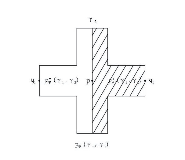
Figure 4. $P^{+}_{\psi}(\gamma_{1},\gamma_{2})$ and $P^{-}_{\psi}(\gamma_{1},\gamma_{2})$ in the plumbing space of $T^{*}\gamma_{1}$ and $T^{*}\gamma_{2}$

Clearly, we have $T^{*}\gamma_{1}=T^{*}\gamma_{1}^{+}\cup T^{*}\gamma_{1}^{-}$ and $T^{*}\gamma_{2}=T^{*}_{+}\gamma_{2}\cup T^{*}_{-}\gamma_{2}$. Denote

$$P_{\psi}^{+}(\gamma_{1},\gamma_{2})=T^{*}\gamma_{1}^{+}\cup_{\psi}T^{*}_{+}\gamma_{2},\quad P_{\psi}^{-}(\gamma_{1},\gamma_{2})=T^{*}\gamma_{1}^{-}\cup_{\psi}T^{*}_{-}\gamma_{2}.$$

Then $P_{\psi}(\gamma_{1},\gamma_{2})=P_{\psi}^{+}(\gamma_{1},\gamma_{2})\cup P_{\psi}^{-}(\gamma_{1},\gamma_{2})$ and $\gamma_{2}=P_{\psi}^{+}(\gamma_{1},\gamma_{2})\cap P_{\psi}^{-}(\gamma_{1},\gamma_{2})$.

We define the rotation map $\mathcal{R}:P_{\psi}^{+}(\gamma_{1},\gamma_{2})\to P_{\psi}(S_{1},S_{2})$ by (see (5.5) for $\bar{\mathcal{R}}$)

$$\mathcal{R}(z)=\begin{cases}\bar{\mathcal{R}}^{1}(z)\;\hbox{if}\;z\in T^{*}\gamma_{1}^{+};\\ \bar{\mathcal{R}}^{2}(z)\;\hbox{if}\;z\in T^{*}_{+}\gamma_{2}.\end{cases}$$

The image of $\mathcal{R}$ is precisely $P_{\psi}^{-}(\gamma_{1},\gamma_{2})$. By Lemma 7.2,

$$\mathcal{R}\big{(}\tau^{n}(\gamma_{2})\cap P_{\psi}^{+}(\gamma_{1},\gamma_{2})\big{)}=\tau^{n}(\gamma_{2})\cap P_{\psi}^{-}(\gamma_{1},\gamma_{2}),$$

and hence, $\tau^{n}(\gamma_{2})$ is invariant under the map $\mathcal{R}$. Note that $\gamma_{1}$ is also invariant under $\mathcal{R}$. So both $\gamma_{1}$ and $\tau^{n}(\gamma_{2})$ belong to $\mathcal{C}_{ad}$, and all bigons of $\gamma_{1}$ and $\tau^{n}(\gamma_{2})$ appear in pairs related by $\mathcal{R}$. Let $q_{1}$ and $q_{2}$ be the antipodal points of the plumbing point $p$ in $S_{1}$ and $S_{2}$ respectively. Denote $\Sigma=\{p,q_{1},q_{2}\}$. As a map on $P_{\psi}(\gamma_{1},\gamma_{2})$, each symplectic Dehn twist $\tau_{i}$ satisfies $\tau_{i}(\Sigma)=\Sigma$, hence the curve $\tau^{n}(\gamma_{2})$ contains precisely two elements of $\Sigma$. Then all bigons $\Omega$ of $\gamma_{1}$ and $\tau^{n}(\gamma_{2})$ are divided into three types:

1. $\Omega\cap\Sigma=\{p,q_{1}\}$;

2. $\Omega\cap\Sigma=\{p\}$ or $\{q_{1}\}$;

3. $\Omega\cap\Sigma=\emptyset$.

Let $D_{+}$ and $D_{-}=\mathcal{R}(D_{+})$ be a pair of such bigons. If $\gamma_{1}$ and $\tau^{n}(\gamma_{2})$ has a bigon of type I, then $\tau^{n}(\gamma_{2})$ contains a simple closed curve homotopic to $\gamma_{1}$ and thus $\tau^{n}(\gamma_{2})$ itself is homotopic to $\gamma_{1}$. If $D_{+}$ and $D_{-}$ are of type II or type III, one can eliminate these two bigons by deforming $\gamma_{1}$ to an isotopic curve $\gamma_{1}^{\prime}\in\mathcal{C}_{ad}$ with $p$ and $q_{1}$ being fixed as illustrated in the Figure 5. ∎

Figure 5. Deforming $\gamma_{1}$ to eliminate the bigons

The last lemma enables us to complete the proof of Lemma 6.4.

Proof of Lemma 6.4.

For the two simple closed curves $\tau^{n}(\gamma_{2}),\gamma_{1}:\mathbb{R}/\mathbb{Z}\to P_{\psi}(\gamma_{1},\gamma_{2})$, whenever $\tau^{n}(\gamma_{2})$ and $\gamma_{1}$ are not isotopic, by successively killing the unnecessary intersection points we can find an isotopy

$$h:[0,1]\times\mathbb{R}/\mathbb{Z}\longrightarrow P_{\psi}(\gamma_{1},\gamma_{2}),\quad h(0,t)=\gamma_{1}(t),\;h(1,t)=\gamma_{1}^{\prime}(t)$$

satisfying the following properties: during the isotopy each $h_{s}=h(s,\cdot)$ is a simple closed curve containing $\{p,q_{1}\}$, and $\gamma_{1}^{\prime}$ and $\tau^{n}(\gamma_{2})$ are transverse and in minimal position in $P_{\psi}(\gamma_{1},\gamma_{2})$, and the image of each $h_{s}$ is invariant under $\mathcal{R}$.

Then by Lemma 7.1 the Lagrangian spheres $S_{1}^{\prime}=L_{\gamma_{1}^{\prime}}$ and $S_{1}$ are Lagrangian isotopic via $L_{h_{s}}$, and hence exact Lagrangian isotopic because of $H^{1}(\mathbb{S}^{n},\mathbb{R})=0$ with $n\geq 2$. As before, the condition (C1) of Theorem 6.1 for $S_{1}^{\prime}$ and $\tau^{n}(S_{2})$ are still satisfied. Since $S_{1}^{\prime}\cap M^{\iota}=\gamma_{1}^{\prime}$ and $\tau^{n}(S_{2})\cap M^{\iota}=\tau^{n}(\gamma_{2})$, by Lemma 7.4 the condition (C2) of Theorem 6.1 for $S_{1}^{\prime}$ and $\tau^{n}(S_{2})$ holds. Then by Theorem 6.1 we have

(7.4) $$\mathrm{rank}\mathrm{HF}\big{(}S_{1},\tau^{n}(S_{2})\big{)}=\mathrm{rank}\mathrm{HF}\big{(}S_{1}^{\prime},\tau^{n}(S_{2})\big{)}=\mathrm{rank}H^{*}(C,\mathbb{Z}/2),$$

where $C=S_{1}^{\prime}\cap\tau^{n}(S_{2})$ and $C^{\iota}=\gamma_{1}^{\prime}\cap\tau^{n}(\gamma_{2})$. Replacing $\gamma_{1}$ by $\gamma_{1}^{\prime}$ in (7.3), we find that if $z\in C^{\iota}\setminus\{p,q_{1}\}$ then the corresponding connected component of $C$ is a sphere and thus its contribution to $\mathrm{rank}H^{*}(C,\mathbb{Z}/2)$ is $2$, and if $z\in\{p,q_{1}\}$ then its contribution is $1$. Since $\gamma_{1}^{\prime}$ and $\tau^{n}(\gamma_{2})$ are invariant under $\mathcal{R}$, the intersection points of $\gamma_{1}^{\prime}$ and $\tau^{n}(\gamma_{2})$ appear in pairs except for $\{p,q_{1}\}\subset C^{\iota}$. So we get $\mathrm{rank}H^{*}(C,\mathbb{Z}/2)=i\big{(}[\gamma_{1}^{\prime}],[\tau^{n}(\gamma_{2})]\big{)}.$ This, together with (7.4), implies the statement.

∎

8. Speculations on Measure theoretic entropy

Since Dehn twists are symplectomorphisms on the manifold $M$, they also preserve the Lebesgue measure $\mu$ on $M$. We conjecture that the measure theoretic entropy of $\tau=\tau_{1}^{k}\tau_{2}^{\ell},kl<0$ on $P_{\psi}(S_{1},S_{2})$ with respect to $\mu$ is also positive. However, there are certain substantial obstacles, similar to the ones we see for the standard map.

Let us first point out the difficulty in the standard map for the purpose of comparison with the current setting. In [9] the authors adopted a special form of a class of 2 dimensional maps including the standard map: $F(x,y)=(y+L\psi(x),-x)$ defined on the torus, where $L$ is a parameter and $\psi$ is a generic smooth function on $\mathbb{T}^{1}$. The derivative matrix has the form $DF(x,y)=\left[\begin{array}[]{cc}L\psi^{\prime}(x)&1\\ -1&0\end{array}\right]$. For large $L$ in most part of the domain ($\{|\psi^{\prime}(x)|>L^{-1/2}\}$), the matrix has a large eigenvalue with almost horizontal eigenvector. However, when $L\psi^{\prime}(x)$ is close to zero, the matrix $DF$ is almost a rotation by $\pi/2$, which can mix expanding and contracting directions.

We shall see below that similar problem appears in our composite Dehn twists in a disguised form.

8.1. Periodic points

We consider the action of $\tau=\tau_{1}\tau_{2}^{-1}$ on $P_{\psi}(S_{1},S_{2})$ for $dim(S_{1})=dim(S_{2})=2$ and for any monotone $r(t)$. Before trying to caculate Lyapunov exponents on the whole manifold, we first consider the Lyapunov exponents at the periodic points, which are given by the eigenvalues of the differential of iterations.

Proposition 8.1.

There exist finitely many $1$-dimensional periodic circles on $P_{\psi}(S_{1},S_{2})$ on which the Lyapunov exponent of $\tau_{1}\tau_{2}^{-1}$ is zero.

Proof.

We notice that $(q,v)\in T^{*}S_{1}$ is a periodic point of $\tau_{1}$ if and only if $r(|v|)\in\mathbb{Q}\pi$. Thus if a point $p_{0}=(q_{2},s_{2})=\psi(q_{1},s_{1})\in P_{\psi}(S_{1},S_{2}),(q_{1},s_{1})\in T^{*}S_{1},(q_{2},s_{2})\in T^{*}S_{2}$ satisfies $r(|s_{i}|)\in\mathbb{Q}\pi,r(|s_{i}|)>2\epsilon,i=1,2$, then $p_{0}$ is a periodic point under $\tau$. For such periodic points, we explicitly calculate the differentials of the Dehn twist in local coordinates.

We consider the plumbing space $P_{\psi}(S_{1},S_{2})$ plumbed at the point $p=(0,0,1)\in S_{i}\subset\mathbb{R}^{3}$, given by local coordinates $\phi_{i}:S_{i}\to\mathbb{R}^{2}$ given by $\phi_{i}(x_{1},x_{2},x_{3})=(x_{1},x_{2})$, and $T^{*}\phi_{i}(x_{1},x_{2},x_{3},y_{1},y_{2},y_{3})=(x_{1},x_{2},y_{1}-\frac{x_{1}y_{3}}{x_{3}},y_{2}-\frac{x_{2}y_{3}}{x_{3}})$. We also suppose that $r^{\prime}\leq\frac{C}{\epsilon}$ for some constant $C$.

So if $\tau_{1}^{k}(p)\in U_{1}$ for $p\in U_{1}$, take $\phi_{1}(p)=(u,v)\in\mathbb{R}^{4},u,v,\in\mathbb{R}^{2}$, then we have, in local coordinates

$$\tilde{\tau_{1}}^{k}(u,v):=\phi_{1}\tau_{1}^{k}\phi_{1}^{-1}(u,v)=\bigg{(}f_{1}(u,v)u+\frac{\sin(kr(\rho))}{\rho}v,\bigg{(}f_{2}(u,v)-\frac{f_{2}}{f_{1}}\bigg{)}u+\cos(kr(\rho))v\bigg{)},$$

where $\rho(u,v)=\sqrt{|v|^{2}-\frac{\langle u,v\rangle^{2}}{1-|u|^{2}}+\frac{\langle u,v\rangle^{2}|u|^{2}}{(1-|u|^{2})^{2}}}$ and

$$f_{1}(u,v)=\cos kr(\rho)-\frac{\sin kr(\rho)}{\rho}\frac{\langle u,v\rangle}{1-|u|^{2}};f_{2}(u,v)=-\sin kr(\rho)\rho-\cos kr(\rho)\frac{\langle u,v\rangle}{1-|u|^{2}}.$$

Suppose $\tau_{1}^{k}(\phi_{1}(u,v))\in U_{1}$, then treating $u,v\in\mathbb{R}^{2}$ as column vectors, when $(u,v)=\phi_{1}^{-1}(p_{0})$ with $p_{0}$ a periodic point of $\tau_{1}$ with period $k$, we have

(8.1) $$\begin{split}d\tilde{\tau_{1}}^{k}(u,v)=\left(\begin{pmatrix}I&0\\ 0&I\end{pmatrix}-\begin{pmatrix}0&\frac{kr^{\prime}}{\rho}\\ -kr^{\prime}\rho&0\end{pmatrix}\begin{pmatrix}\frac{\partial\rho}{\partial u}u^{t}&\frac{\partial\rho}{\partial v}u^{t}\\ \frac{\partial\rho}{\partial u}v^{t}&\frac{\partial\rho}{\partial v}v^{t}\end{pmatrix}\right.\\ \left.+\frac{\langle u,v\rangle}{1-|u|^{2}}\begin{pmatrix}\frac{kr^{\prime}}{\rho}\frac{\partial\rho}{\partial u}u^{t}&\frac{kr^{\prime}}{\rho}\frac{\partial\rho}{\partial v}u^{t}\\ -1+\frac{\langle u,v\rangle}{1-|u|^{2}}\frac{kr^{\prime}}{\rho}\frac{\partial\rho}{\partial u}u^{t}&\frac{\langle u,v\rangle}{1-|u|^{2}}\frac{kr^{\prime}}{\rho}\frac{\partial\rho}{\partial v}u^{t}\end{pmatrix}\right)\begin{pmatrix}du\\ dv\end{pmatrix}.\end{split}$$

Furthermore, if we suppose $\phi(p_{0})=(u,v)$ with $\langle u,v\rangle=0$, then we have the exact equality

$$d\tilde{\tau_{1}}^{k}(u,v)=\begin{pmatrix}I&kr^{\prime}(|v|)\hat{v}\hat{v}^{t}\\ 0&I\end{pmatrix}\begin{pmatrix}du\\ dv\end{pmatrix}$$

where we write $\hat{v}=\frac{v}{|v|}$.

Next we consider the action of the second Dehn twist $\tau_{2}$, suppose $p_{0}$ is a periodic point of $\tau_{2}$ of period $\ell$. Since the coordinates $(u,v)$ on $T^{*}S_{1}$ is identified to coordinates $(u^{\prime},v^{\prime})$ on $T^{*}S_{2}$ through $J:(u,v)\to(u^{\prime},v^{\prime})=(-v,u)$, we have

$$d(J^{-1}\phi_{2}\tau_{2}\phi_{2}^{-1}J)^{\ell}(u^{\prime},v^{\prime})=\begin{pmatrix}0&I\\ -I&0\end{pmatrix}\begin{pmatrix}I&\ell r^{\prime}(|u|)\hat{u}\hat{u}^{t}\\ 0&I\end{pmatrix}\begin{pmatrix}0&-I\\ I&0\end{pmatrix}\begin{pmatrix}du\\ dv\end{pmatrix}$$

$$=\begin{pmatrix}I&0\\ -\ell r^{\prime}(|u|)\hat{u}\hat{u}^{t}&I\end{pmatrix}\begin{pmatrix}du\\ dv\end{pmatrix}.$$

Now we calculate the differential of an iteration of $\tau$ at $p_{0}\in T^{*}U_{1}\cap T^{*}U_{2}\subset P_{\psi}(S_{1},S_{2})$. Suppose $p_{0}=(q_{2},s_{2})=\psi(q_{1},s_{1})\in P_{\psi}(S_{1},S_{2}),(q_{1},s_{1})\in T^{*}S_{1},(q_{2},s_{2})\in T^{*}S_{2}$ with $r(|s_{1}|)=\frac{1}{k}\geq 2\epsilon,r(|s_{2}|)=\frac{1}{l}\geq 2\epsilon$, then $p_{0}$ is also a periodic point of $\tau_{1}\tau_{2}^{-1}$, of period $k+|\ell|-1$. By the calculations above, we see that for $p_{0}=\phi^{-1}(u,v)$ with $\langle u,v\rangle=0$, we have

$$d(\tau_{1}\tau_{2}^{-1})^{k+\ell-1}(u,v)=d(\tau_{1}^{k})d(\tau_{2}^{-l})(u,v)=\begin{pmatrix}I&kr^{\prime}(|v|)\hat{v}\hat{v}^{t}\\ \ell r^{\prime}(|u|)\hat{u}\hat{u}^{t}&I\end{pmatrix}\begin{pmatrix}du\\ dv\end{pmatrix}.$$

Thus $d(\tau_{1}\tau_{2}^{-1})^{k+\ell-1}(u,v)$ has eigenvalues 1, so we have $\chi^{+}(p_{0})=0$ for finitely many $p_{0}$.

∎

8.2. Hyperbolic cones near the elliptic points

Now if we remove the condition $\langle u,v\rangle=0$ for $p_{0}$ and keep the conditions that $p_{0}$ is periodic under both $\tau_{1}$ and $\tau_{2}$ we would get a partially hyperbolic periodic point of $\tau$. However, we shall see that in a neighborhood of the elliptic periodic point, the eigenvectors of the hyperbolic periodic points “flip”, so the arguments we used in Section 4 to prove positive measure theoretic entropy on the subsystem cannot be applied to prove positive entropy on the whole system with respect to the Lebesgue measure.

Now for $p_{0}=(q_{2},s_{2})=\psi(q_{1},s_{1})\in P_{\psi}(S_{1},S_{2}),(q_{1},s_{1})\in T^{*}S_{1},(q_{2},s_{2})\in T^{*}S_{2}$ with $r(|s_{i}|\in\mathbb{Q},r(|s_{i}|)>2\epsilon,i=1,2$, we see from the second condition that $|u|,|v|<\epsilon$, which gives us

$$d\tilde{\tau_{1}}^{k}(u,v)=\left(\begin{pmatrix}I&kr^{\prime}(|v|)\hat{v}\hat{v}^{t}\\ 0&I\end{pmatrix}+O(\langle u,v\rangle)\right)\begin{pmatrix}du\\ dv\end{pmatrix}.$$

Applying the same argument for $\tau_{2}$, we have

$$d\tilde{\tau_{2}}^{\ell}(u,v)=\left(\begin{pmatrix}I&0\\ -\ell r^{\prime}(|u|)\hat{u}\hat{u}^{t}&I\end{pmatrix}+O(\langle u,v\rangle)\right)\begin{pmatrix}du\\ dv\end{pmatrix}.$$

Thus $p_{0}$ as also a periodic point of $\tau_{1}\tau_{2}^{-1}$ of period $k+|\ell|-1$ has differential

$$d(\tau_{1}\tau_{2}^{-1})^{k+\ell-1}(u,v)=\left(\begin{pmatrix}\ell+k\ell r^{\prime}(|u|)r^{\prime}(|v|)\langle\hat{u},\hat{v}\rangle\hat{v}\hat{u}^{t}&kr^{\prime}(|v|)\hat{v}\hat{v}^{t}\\ \ell r^{\prime}(|u|)\hat{u}\hat{u}^{t}&I\end{pmatrix}+O(\langle u,v\rangle/\epsilon)\right)\begin{pmatrix}du\\ dv\end{pmatrix}.$$

Thus for $p_{0}=\phi_{1}(u,v)$ with $\langle u,v\rangle\neq 0$, we have $tr(d(\tau_{1}\tau_{2}^{-1})^{k+\ell-1})>4$ which shows that $p_{0}$ has positive Lyapunov exponent. The eigenvalues of $d(\tau_{1}\tau_{2}^{-1})^{k+\ell-1}$ are approximately

$$\lambda_{1}=1+\ell r^{\prime}(|u|)\langle\hat{u},\hat{v}\rangle\frac{k\ell r^{\prime}(|u|)r^{\prime}(|v|)\langle\hat{u},\hat{v}\rangle+\sqrt{(k\ell r^{\prime}(|u|)r^{\prime}(|v|)\langle\hat{u},\hat{v}\rangle)^{2}+4(kr^{\prime}(|v|))^{2}}}{2},$$

$$\lambda_{2}=\lambda_{3}=1,$$

$$\lambda_{4}=1+\ell r^{\prime}(|u|)\langle\hat{u},\hat{v}\rangle\frac{k\ell r^{\prime}(|u|)r^{\prime}(|v|)\langle\hat{u},\hat{v}\rangle-\sqrt{(k\ell r^{\prime}(|u|)r^{\prime}(|v|)\langle\hat{u},\hat{v}\rangle)^{2}+4(kr^{\prime}(|v|))^{2}}}{2}$$

with eigenvectors

$$w_{1}=\begin{pmatrix}\frac{k\ell r^{\prime}(|u|)r^{\prime}(|v|)\langle\hat{u},\hat{v}\rangle+\sqrt{(k\ell r^{\prime}(|u|)r^{\prime}(|v|)\langle\hat{u},\hat{v}\rangle)^{2}+4(kr^{\prime}(|v|))^{2}}}{2}\hat{v}\\ \hat{u}\end{pmatrix}$$

and

$$w_{4}=\begin{pmatrix}\frac{k\ell r^{\prime}(|u|)r^{\prime}(|v|)\langle\hat{u},\hat{v}\rangle-\sqrt{(k\ell r^{\prime}(|u|)r^{\prime}(|v|)\langle\hat{u},\hat{v}\rangle)^{2}+4(kr^{\prime}(|v|))^{2}}}{2}\hat{v}\\ \hat{u}\end{pmatrix}.$$

So we see that if $\langle u,v\rangle>0$ we have $\lambda_{1}>1$ and $\lambda_{4}<1$, and when $\langle u,v\rangle<0$ we have $\lambda_{1}<1$ and $\lambda_{4}>1$. However the corresponding eigenvectors $w_{1}$ and $w_{4}$ is continuous with respect to $u,v$. Thus if a tangent vector returns to the neighborhood of an elliptic periodic point, it can start shrinking even if it was originally expanding.

Appendix A Topological entropy and nonuniformly hyperbolic dynamics

Here we introduce the basic definitions of topological and measure theoretic entropy and its relation to hyperbolicity of the system. The contents of this subsection is classical and can be found in e.g. Chapters 3, 4 and Supplement of [19].

Definition A.1 (Topological entropy).

The topological entropy of a map $f:X\to X$ on a compact metric space $(X,d)$ is given by

$$h_{d}(f)=\lim_{\delta\to 0}\limsup_{n\to\infty}\frac{1}{n}\log S_{d}(f,\delta,n)$$

where $S_{d}(f,\delta,n)$ is the minimal cardinality of set of balls $B(x,\delta,d^{f}_{n})$ that covers the space $X$. Here the balls $B(x,\delta,d^{f}_{n})=\{y\in X:d^{f}_{n}(x,y)<\delta\}$ are taken with respect to the metric $d^{f}_{n}(x,y)=\max_{0\leq i\leq n-1}d(f^{i}(x),f^{i}(y))$.

The topological entropy has the following properties.

Proposition A.1.

1. The topological entropy does not depend on the metric $d$. If $d^{\prime}$ is a metric on $X$ such that $(X,d)$ and $(X,d^{\prime})$ has the same topology then $h_{d}(f)=h_{d^{\prime}}(f)$. Thus we define $h_{top}(f)=h_{d}(f)$ for any metric $d$ compatible with the topology.

2. The topological entropy is invariant under conjugacy, i.e. $h_{top}(f)=h_{top}(g^{-1}fg)$ for any homeomorphism $g:X\to Y$.

3. If $\Lambda$ is a closed $f$-invariant subset of $X$, then $h_{top}(f\mid_{\Lambda})\leq h_{top}(f)$.

4. $h_{top}(f^{m})=mh_{top}(f)$.

Definition A.2 (Measure theoretic entropy).

A measurable partition of a probability space $(X,\mathcal{B},\mu)$ is a collection of measurable subsets $\xi=\{C_{\alpha}\in\mathcal{B}\ |\ \alpha\in I\}$ such that $\mu(\cup C_{\alpha})=1$ and $\mu(C_{\alpha}\cap C_{\beta})=0\text{ or }\mu(C_{\alpha}\Delta C_{\beta})=0,\forall\alpha\neq\beta$.

The entropy of a measurable partition $\xi=\{C_{\alpha}\in\mathcal{B}\ |\ \alpha\in I\}$ is given by

$$H(\xi)=-\sum_{\alpha\in I}\mu(C_{\alpha})\log(\mu(C_{\alpha})).$$

The entropy of a measure-preserving transformation $T$ on $(X,\mu)$ is defined as

$$h_{\mu}(T)=\sup_{\xi}\lim_{n\to\infty}\frac{1}{n}H(\{\cap_{i=1}^{n}T^{-i+1}C_{i}\ |\ C_{i}\in\xi\})$$

where $\xi$ is taken over any measurable partition with $H(\xi)<\infty$.

The measure theoretic entropy and the topological entropy of are related by the variational principle.

Theorem A.2 (Variational Principle).

Let $X$ be a compact metric space, $f:X\to X$ a homeomorphism. Set $M(f)$ to be the set of Borel probability measures that are $f$-invariant. Then we have

$$h_{top}(f)=\sup_{\mu\in M(f)}h_{\mu}(f).$$

One way of calculating measure theoretic entropy is by examining the “hyperbolicity” of the map $f$. As we shall see in Pesin entropy formula, a diffeomorphism $f$ has positive entropy if it possesses some hyperbolicity. A diffeomorphism $f:X\to X$ on a Riemannian manifold is said to be hyperbolic if a every point $p$, $Df$ expands a subspace $E^{+}(p)\subset T_{p}X$ at rate $\lambda>1$ and contracts a subspace $E^{-}(p)\subset T_{p}X$ at rate $1/\lambda<1$ such that $T_{p}X=E^{+}(p)\oplus E^{-}(p)$ and $E^{+},E^{-}$ are invariant under $f$.

A more precise description of hyperbolicity at a generic point is given by the Lyapunov exponent which describes the expansion rate of $f$ on a tangent vector $(p,u)$.

Definition A.3.

Let $X$ be a Riemannian manifold with $f:X\to X$ a diffeomorphism of $X$. The Lyapunov exponent of $f$ at a point $(p,u)\in TX$ is defined as

$$\chi^{+}(p,u)=\lim_{m\to\infty}\frac{1}{m}\log\|df^{m}_{p}(u)\|$$

if the limit exists.

Although a priori the Lyapunov exponent of a tangent vector may not exist, Oseledets [19] proved that for almost every point on the manifold $X$ the Lyapunov exponent at any vector is well defined, and we can split the tangent space into subspaces on which $f$ has uniform hyperbolicity.

Theorem A.3 (Oseledets Multiplicative Ergodic Theorem).

Let $X$ be a Riemannian manifold with $f:X\to X$ a diffeomorphism, let $\mu$ be a $f$-invariant Borel measure on $X$ such that $\log^{+}\|Df(\cdot)\|\in L^{1}(X,\mu)$, then there exists a set $Y\subset X$ with $\mu(X\backslash Y)=0$ such that for each $p\in Y$, there exists a decomposition $T_{p}X=\oplus_{i=1}^{k(p)}H_{i}(p)$ that is invariant under $Df$ and a set of $f$-invariant functions $\chi_{1}(p)<\chi_{2}(p)<...<\chi_{k(p)}(p)$ $($called the Lyapunov exponents of $p)$ such that the Lyapunov exponent exists for any $u\in T_{p}X$ and $\chi^{+}(p,u)=\pm\chi_{i}(p),\ \forall\ u\in H_{i}(p).$

Furthermore, we can use the splitting of the tangent spaces to generate stable and unstable local submanifolds of a non-uniformly hyperbolic map. Here, to avoid technical details, we only state the result for Riemannian surfaces which we shall use in section 1.2. More details on this subject can be found in Chapter 7 and 8 [6].

Theorem A.4 (Pesin’s stable manifold theorem[6]).

Let $X$ be a Riemannian surface and $f:X\to X$ a diffeomorphism such that the Lyapunov exponent $\chi_{1}(p)<0$ for almost every $p\in X$, then there exists Borel functions $C:X\to\mathbb{R}$ and $\lambda:X\to(0,1)$, such that for almost every $p\in X$, there exists a stable manifold $($curve$)$ $W^{s}_{f}(p)$ such that $x\in W^{s}_{f}(p),T_{p}W^{s}(p)=H_{1}(p)$, and for any $q\in W^{s}_{f}(p)$ we have

$$\mathrm{dist}(f^{n}(p),f^{n}(q))\leq C(x)\lambda^{n}(x)\mathrm{dist}(x,y).$$

Furthermore, the stable manifolds satisfy $W^{s}(q)=W^{s}(p)$ for any $q\in W^{s}(p)$ and $W^{s}(q)\cap W^{s}(p)=\varnothing$ if $q\notin W^{s}(p)$.

Similarly, if we consider local stable manifolds $W^{s}_{f^{-1}}(p)$ of $f^{-1}$, then the action of $f$ expands the distance of points on the manifold exponentially. We call them the local unstable manifolds of $f$ and denote by $W^{u}_{f}(p)=W^{s}_{f^{-1}}(p)$.

The Lyapunov exponents is connected with the entropy of a map by the Pesin entropy formula.

Theorem A.5 (Pesin entropy formula).

Let $X$ be a compact Riemannian manifold with $f:X\to X$ a diffeomorphism, suppose that $f$ preserves a smooth Borel measure $\mu$ on $X$, then we have

$$h_{\mu}(f)=\int\chi^{+}d\mu$$

where $\chi^{+}(p)=\sum_{\chi_{i}(p)>0}\chi_{i}(p)$ with $\chi_{i}$ the Lyapunov exponents of $p$ as given in the Osedelec Multiplicative Ergodic Theorem.

Appendix B Floer cohomology

In the section we give a brief review of Lagrangian Floer cohomology. The definition of Floer cohomology here is essentially Floer’s original one [15]. For our purpose in the present paper, we work with ungraded groups.

Let $(\overline{M},d\bar{\lambda})$ be a $2n$-dimensional exact symplectic manifold with contact-type boundary, and let $(M,d\lambda)$ be its symplectization. Let $(S_{1},S_{2})$ be a pair of connected compact exact Lagrangian submanifolds of $M$ with $\lambda|_{S_{i}}=df_{i},i=1,2$, where $f_{i}\in C^{\infty}(S_{i},\mathbb{R})$. The action functional on the path space

$$\mathcal{P}(S_{1},S_{2})=\big{\{}\gamma:[0,1]\to M|\gamma(0)\in S_{1},\gamma(1)\in S_{2}\big{\}}$$

is defined as

$$\mathcal{A}_{S_{1},S_{2}}(\gamma)=\int\gamma^{*}\lambda+f_{1}(\gamma(0))-f_{2}(\gamma(1)).$$

Clearly, the critical points of $\mathcal{A}_{S_{1},S_{2}}$ are constant paths $\gamma_{x}$ at the intersection points $x$ of $S_{1}$ and $S_{2}$. If $S_{1}$ and $S_{2}$ intersect transversely, the Floer cohomology $\mathrm{HF}(S_{1},S_{2})$ is well defined by the standard argument of transversality and gluing, see [24]. In general, to define Floer cohomology one needs to consider Hamiltonian perturbations to achieve transversality. Let us give a quick review of this construction. Let $H\in\mathcal{H}=C^{\infty}([0,1]\times M,\mathbb{R})$. For every $\gamma\in\mathcal{P}(S_{1},S_{2})$, the Hamiltonian action of $\gamma$ is

$$\mathcal{A}_{S_{1},S_{2}}^{H}(\gamma)=\int\gamma^{*}\lambda-\int^{1}_{0}H(t,\gamma(t))dt+f_{1}(\gamma(0))-f_{2}(\gamma(1)).$$

Denote $\mathcal{P}_{H}(S_{1},S_{2})\subset\mathcal{P}(S_{1},S_{2})$ the critical points of this functional, which are the flow lines of the Hamiltonian flow $\phi_{H}^{t}$, i.e., $\gamma:[0,1]\to M$ such that $\dot{\gamma}(t)=X_{H}(t,\gamma(t))$, $\gamma(0)\in S_{1}$ and $\gamma(1)\in S_{2}$. So there is a one-to-one correspondence between $\mathcal{P}_{H}(S_{1},S_{2})$ and $\phi^{1}_{H}(S_{1})\cap S_{2}$. For generic $H\in\mathcal{H}^{reg}\subseteq\mathcal{H}$, $\phi^{1}_{H}(S_{1})$ and $S_{2}$ intersect transversely. The Floer cochain $CF(S_{1},S_{2})$ is the vector space over $\mathbb{Z}/2$ with a base given by these intersection points. Denote by $\mathcal{J}$ the set of one-parameter families $(J_{t})_{0\leq t\leq 1}$ of almost complex structures on $M$ such that each $J_{t}$ is $d\lambda$-compatible, and is independent of $t$ and tame at infinity (for the definition of “tame” see [7]). For $J\in\mathcal{J}$, consider the maps $u:\mathbb{R}\times[0,1]\to M$ which solves the perturbed Cauchy-Riemannian equation

(B.1) $$\partial_{s}u+J(t,u)\big{(}\partial_{t}u-X_{H}(t,u)\big{)}=0$$

subject to the boundary conditions

$$u(s,0)\in S_{1}\;\hbox{and}\;u(s,1)\in S_{2},\quad s\in\mathbb{R}$$

$$\lim\limits_{s\to+\infty}u(s,t)=x,\qquad\lim\limits_{s\to+\infty}u(s,t)=y$$

and the finite energy condition

$$E(u)=\frac{1}{2}\int^{1}_{0}\int^{1}_{0}\big{|}\partial_{s}u\big{|}^{2}+\big{|}\partial_{t}u-X_{H}(u)\big{|}^{2}dsdt<\infty.$$

Denote by $\widehat{\mathcal{M}}(x,y;H,J)$ the space of the above maps $u$. There is a natural $\mathbb{R}$-translation on $\widehat{\mathcal{M}}(x,y;H,J)$ in $s$-direction, and its quotient space is denoted by $\mathcal{M}(x,y;$ $H,J)$. Solutions of (B.1) can be thought as negative gradient flow lines for $\mathcal{A}_{S_{1},S_{2}}^{H}$ in an $L^{2}$-metric on $\mathcal{P}(S_{1},S_{2})$. For each $u\in\widehat{\mathcal{M}}(x,y;H,J)$ we linearize (B.1) and obtain a Fredholm operator $D_{H,J,u}$ in suitable Sobolev spaces. Under the assumptions that $\langle[\omega],\pi_{2}(M,S_{i})\rangle=0,i=1,2$, there is a dense subspace $\mathcal{J}^{reg}\subset\mathcal{J}$ of almost complex structures such that $D_{H,J,u}$ are onto for all $u\in\widehat{\mathcal{M}}(x,y;H,J)$, see [15]. Hence the spaces $\widehat{\mathcal{M}}(x,y;H,J)$, as well as $\mathcal{M}(x,y;H,J)$, are smooth manifolds.

In the setting of our present paper, these topological assumptions are met, and then we can define the Floer differential $d_{H,J}:\ \mathrm{CF}(S_{1},S_{2})\to\mathrm{CF}(S_{1},S_{2})$ by counting isolated points in $\mathcal{M}(x,y;H,J)$ mod $2$, i.e.,

$$d_{H,J}(y)=\sum_{x}\sharp_{2}\mathcal{M}(x,y;H,J)x.$$

This map has square zero, i.e., $d_{H,J}^{2}=0$, and hence $\mathrm{CF}(S_{1},S_{2})$ is a complex over the coefficient $\mathbb{Z}/2$. $\mathrm{HF}(S_{1},S_{2})$ is defined to be its cohomology $\mathrm{Ker}(d_{H,J})/\mathrm{Im}(d_{H,J})$. It can be shown that Floer cohomology $\mathrm{HF}(S_{1},S_{2})$ is independent of the pair $(H,J)$ up to canonical isomorphism, see [28, 30].

References

- [1] M. Abouzaid, A topological model for the Fukaya categories of plumbings, J. Differential Geom. 87 (2011), 1–80.
- [2] V. I. Arnold, Some remarks on symplectic monodromy of Milnor fibrations, The Floer Memorial Volume (H. Hofer, C. Taubes, A. Weinstein, and E. Zehnder, eds.), Progress in Mathematics, vol. 133, Birkhäuser, 1995, pp. 99-104.
- [3] V. I. Arnold, Dynamics of complexity of intersections. Bol. Soc. Brasil. Mat. (N.S.) 21 (1990), 1–10.
- [4] Shaoyun Bai, Paul Seidel, Injectivity of twisted open-closed maps, in preparation.
- [5] F. Barbacovi, J. Kim, Entropy of the composition of two spherical twists, Arxiv: 2107.06079.
- [6] L. Barreira, Y. Pesin. Nonuniform Hyperbolicity: Dynamics of Systems with Nonzero Lyapunov Exponents. Encyclopedia of Mathematics and Its Applications, 115 Cambridge University Press.
- [7] M. Audin and J. Lafontaine (Eds), Holomorphic curves in symplectic geometry, Progress in Mathematics, Birkhäuser Verlag, Basel, 117 (1994).
- [8] R. Burton and R. W. Easton. Ergodicity of linked twist maps. In Global theory of dynamical systems (Proc. Internat. Conf., Northwestern Univ., Evanston, Ill., 1979), volume 819 of Lecture Notes in Math., pages 35–49. Springer, Berlin, 1980.
- [9] A. Blumenthal, J. Xue, L.-S. Young, Lyapunov exponents for random perturbations of some area-preserving maps including the standard map, Ann. Math. 185 (2017), 285-310
- [10] G. Dimitrov, F. Haiden, L. Katzarkov, and M. Kontsevich, Dynamical systems and categories, Contemp. Math. 621 (2014), 133-170.
- [11] Y-W. Fan, S. Filip, F. Haiden, L. Katzarkov, and Y. Liu, On pseudo-Anosov autoequivalences Adv. Math., 384 (2021),
- [12] B. Farb and D. Margalit. A primer on mapping class groups, volume 49 of Princeton Mathematical Series. Princeton University Press, Princeton, NJ, 2012.
- [13] A. Fathi. Dehn twists and pseudo-Anosov diffeomorphisms. Invent. Math., 87(1):129–151, 1987.
- [14] A. Fathi, F. Laudenbach and V. Poénaru, editors. Travaux de Thurston sur les surfaces, volume 66 of Astérisque. Société Mathématique de France, Paris, 1979.
- [15] A. Floer, Morse theory for Lagrangian intersections, J. Differential Geom. 28 (1988), 513–547.
- [16] A. Floer, Witten’s complex and infinite dimensional Morse theory, J. Differential Geom. 30 (1989), 207–221.
- [17] U. Frauenfelder and F. Schlenk, Volume growth in the component of the Dehn-Seidel twist, Geom. Funct. Anal. 15 (2005), 809–838.
- [18] A. Jannaud, Dehn-Seidel twist, -symplectic topology and barcodes. arXiv:2101.07878.
- [19] A. Katok and B. Hasselblatt. Introduction to the modern theory of dynamical systems, volume 54 of Encyclopedia of Mathematics and its Applications. Cambridge University Press, Cambridge, 1995. With a supplementary chapter by Katok and Leonardo Mendoza.
- [20] A. M. Keating, Dehn twists and free subgroups of symplectic mapping class groups, J. Topol. 7 (2014), 436–474.
- [21] K. Kikuta and G. Ouchi. Hochschild entropy and categorical entropy. 2020. ArXiv:2012.13510.
- [22] M. Khovanov and P. Seidel, Quivers, Floer cohomology, and braid group actions. J. Amer. Math. Soc. 15 (2002), 203–271.
- [23] S. Lee, Towards a higher-dimensional construction of stable/unstable Lagrangian laminations. Arxiv: 1903.09472.
- [24] Y.-G. Oh, Symplectic topology as the geometry of the action functional I, J. Differential Geom. 46 (1977) 1–55.
- [25] R. C. Penner, A construction of pseudo-Anosov homeomorphisms. Trans. Amer. Math. Soc. 310 (1988) 179–197.
- [26] M. Poźniak, Floer homology, Novikov rings, and clean intersections. Northern California Symplectic Geometry Seminar, Amer. Math. Soc. Transl., Ser. 2, 196, AMS, Providence, 1999, 119-181.
- [27] L. Polterovich and E. Shelukhin, Autonomous Hamiltonian flows, Hofer’s geometry and persistence modules, Selecta Mathematica volume 22, pages227-296 (2016)
- [28] D. Salamon and E. Zehnder, Morse theory for periodic solutions of Hamiltonian systems and the Maslov index, Comm. Pure Appl. Math. 45 (1992), 130–1360.
- [29] P. Seidel, Lagrangian two-spheres can be symplectically knotted, J. Differential Geom. 52 (1999), 147–173.
- [30] P. Seidel, A long exact sequence for symplectic Floer cohomology, Topology 42 (2003), 1003–1063.
- [31] P. Seidel, Lectures on Categorical Dynamics and Symplectic Topology
- [32] W. P. Thurston, On the geometry and dynamics of diffeomorphisms of surfaces, Bull. Amer. Math. Soc. (N.S.) 19 (1988), no. 2, 417-431.
- [33] W. Wu. Exact Lagrangians in -surface singularities. Math. Ann., 359(1-2):153–168, 2014.