Generally–Altered, –Inflated, –Truncated and –Deflated Regression, With Application to Heaped and Seeped Data

Abstract   Models such as the zero-inflated and zero-altered Poisson and zero-truncated binomial are well-established in modern regression analysis. We propose a super model that jointly and maximally unifies alteration, inflation, truncation and deflation for counts, given a 1- or 2-parameter parent (base) distribution. Seven disjoint sets of special value types are accommodated because all but truncation have parametric and nonparametric variants. Some highlights include: (i) the mixture distribution is exceeding flexible, e.g., up to seven modes; (ii) under-, equi- and over-dispersion can be handled using a negative binomial (NB) parent, with underdispersion handled by a novel Generally-Truncated-Expansion method; (iii) overdispersion can be studied holistically in terms of the four operators; (iv) an important application: heaped and seeped data from retrospective self-reported surveys are readily handled, e.g., spikes and dips which are located virtually anywhere; (v) while generally-altered regression explains why observations are there, generally-inflated regression accounts for why they are there in excess, and generally-deflated regression explains why observations are not there; (vi) the VGAM R package implements the methodology based on Fisher scoring and multinomial logit model (Poisson, NB, zeta and logarithmic parents are implemented.) The GAITD-NB has potential to become the Swiss army knife of count distributions.

Keywords:   Finite mixture distribution; Fisher scoring; iteratively reweighted least squares algorithm; multinomial logit model; negative binomial regression; overdispersion and underdispersion; spliced distribution; vector generalized linear model.

1 Introduction

The analysis of counts plays an important subtopic in regression theory. Here, the subject of zero-inflation, zero-deflation, zero-truncation, and zero-alteration have gained enormous traction and are now a part of the modern regression analysis toolkit, e.g., Kleiber and Zeileis (2008), Zuur et al. (2012), Cameron and Trivedi (2013), Agresti (2015), Berger and Tutz (2021), and the recent review Haslett et al. (2022). In particular, all four types of operators (“A”, “I”, “D” and “T”) have found rich applications in both Poisson and binomial distribution forms, where the ZIP has been attributed to Lambert (1992) and the ZAP is often described as a hurdle model (Mullahy, 1986). In capture–recapture experiments the absence of 0s leads to conditional models (e.g., Otis et al., 1978) such as the positive Bernoulli distribution or zero-truncated binomial (ZTB); occupancy models (e.g., MacKenzie et al., 2002) also make use of them.

Let ${\cal R}$ be the support of the parent (base) distribution, e.g., $\{0,1,\ldots\}$ for the Poisson. The purpose of this paper is to extend previous work such as the above in three directions:

• Any subset of the support can be altered, inflated, deflated or truncated, cf. treating only the singleton {0} as special. The first three are denoted ${\cal A}$ ${\cal I}$, ${\cal D}$ with finite cardinality. The truncation set ${\cal T}$ may be innumerable so it is merely a proper subset of ${\cal R}$.

• Rather than allowing only one of ${\cal A}$, ${\cal I}$, ${\cal D}$ and ${\cal T}$, the four operators are combined into a single model and are allowed to operate concurrently. This confers greater versatility and a holistic approach. The ${\cal A}$, ${\cal I}$, ${\cal D}$ and ${\cal T}$ are mutually disjoint.

• Utilizing (I)–(II) on ${\cal A}$, ${\cal I}$ and ${\cal D}$, parametric (subscript “$p$”) and nonparametric (“$np$”) forms are spawned, hence there are 7 special value types. These are further combined into a ‘super’ model, which is informally called the GAITD ‘combo’ instead for modesty.

• Although we present (I)–(III) mainly for 1- and 2-parameter count parents (Poisson, negative binomial, logarithmic and zeta) our work is envisaged for continuous distributions.

Altogether, these directions allow a grand unification of the four operators by the combo model which necessitates novel methodology such as a finite mixture distribution with nested support.

1.1 Some Justification

Why are such extensions are so necessary? The following short examples illustrate why it is crucial to be able to inflate, deflate and truncate any set of values and not just $\{0\}$.

• Fig. 1(a) is a spikeplot (Cox, 2004) showing the proportions of self-reported age at which 3263 ex-smokers quit their habit. Two ‘layers’ are apparent. The outer one is on a subset of mainly multiples of 5 and 10. The inner layer might be thought as being the ‘main’ distribution with the outer distribution being similar but sampled at a greater intensity and at selected points. Alternatively, the outer layer might be explained by sampling from the inner distribution at selected points and then added on top of the inner layer.

• Fig. 1(b) spikeplots the length of stay proportions of a large 4-star complex and resort located in the southern Sardinia, Italy. Days 7 and 14 are inflated partly because of discount rates offered to guests who book accommodation in an integral unit of weeks. Comparing days 1 and 2, either the first day is deflated relative to day 2, else the second day is inflated relative to day 1.

• With similarities to Fig. 1(a), Fig. 2 is a spikeplot of self-reported smoking duration. The proportions from these $n=5492$ current or ex-smokers appear to have a heavy-tailed distribution such as the zeta or logarithmic but with many multiples of 5 and 10 years having spikes. The value 12 for a “dozen” may be heaped too. A close examination shows that some inflated values are sandwiched between two deflated values, e.g., 29 and 31 about 30 years. We analyze this data set in Section 6.2.

Likewise, applications that utilize (I) with respect to truncation of any set of values is important for at least two reasons:

1. it is common to truncate the lower and/or upper tail of a distribution. For example, due to physical limits, ${\cal T}$ must theoretically include $\{25,26,\ldots\}$ in Fig. 8(a) as there are only 24 hours per day. Another compelling example is outlier deletion: if observations are removed then the analysis ought to reflect this by generally-truncating those values of the support. The Section 6.1 analysis is such an example;

2. truncation can arise from many diverse situations. For example, tetraphobia in East Asian culture and triskaidekaphobia in Western culture create structural absences in certain sampling units: buildings that omit the 4th floor and public passenger seating that omit row 13 are everyday examples. Fig. 2 are both 0-truncated.

Figure 1: Two spikeplot examples from VGAMdata. (a) Heaped variable smokeagequit in a large cross-sectional study called xs.nz. (b) Flamingo Hotel length of stay (LOS; in days, $n=4871$) from flamingo.

As seen by two of the examples, one very notable application of our technique is the analysis of heaped data, an aberration ubiquitous in surveys especially among self-reported variables (also called ‘digit preference’ data). Frequently seen by an excess of multiples of 5 and 10 relative to other values, it is uncommon for respondents know their exact values, hence regression analyses may suffer from bias due to this form of measurement error (Heitjan and Rubin, 1990; Carroll et al., 2006). While GAITD regression can handle heaped data, its scope is far wider since digit preference is not the only mechanism for generating spikes, e.g, Fig. 1(b). Hence one source of inflation is heaped data and one source of deflation is seeped data—the tendency not to select those values at the expense of the heaped values due to measurement error. We return to the over-/under-representation problem of heaped/seeped data in Section 3.5.

Figure 2: Smoking duration from 5492 current or past smokers in a large cross-sectional study (Variable smokeyears in xs.nz). The fitted GAITD regression is overlaid in Fig. 9.

1.2 Nomenclature and notation

The methodology involves four operators and draws from several areas, therefore it is helpful to summarize most of the notation and nomenclature used throughout here.

Nomenclaturewise due to (II)–(III), the acronym GAITD is used to describe the new models, and abbreviations such as GIT for submodels when $\mbox{${\cal A}$}_{p}=\mbox{${\cal A}$}_{np}=\mbox{${\cal D}$}_{p}=\mbox{${\cal D}$}_{np}=\{\}$. Any altered, inflated, deflated or truncated value is called special and we let ${\cal S}$ be their union. The other values of the support are described as ordinary or nonspecial. Let $\mbox{${\cal T}$}=\{t_{1},t_{2},\ldots\}$, $\mbox{${\cal A}$}_{p}=\{a_{1},\ldots,a_{|\mbox{\scriptsize${\cal A}$}_{p}|}\}$, $\mbox{${\cal A}$}_{np}=\{a_{1},\ldots,a_{|\mbox{\scriptsize${\cal A}$}_{np}|}\}$, $\mbox{${\cal I}$}_{p}=\{i_{1},\ldots,i_{|\mbox{\scriptsize${\cal I}$}_{p}|}\}$, $\mbox{${\cal I}$}_{np}=\{i_{1},\ldots,i_{|\mbox{\scriptsize${\cal I}$}_{np}|}\}$, $\mbox{${\cal D}$}_{p}=\{d_{1},\ldots,d_{|\mbox{\scriptsize${\cal D}$}_{p}|}\}$ and $\mbox{${\cal D}$}_{np}=\{d_{1},\ldots,d_{|\mbox{\scriptsize${\cal D}$}_{np}|}\}$ be an enumeration of the mutually exclusive sets comprising ${\cal S}$. (The notation is imperfect because $i_{1}$ could belong to $\mbox{${\cal I}$}_{p}$ or $\mbox{${\cal I}$}_{np}$, however the context always renders any distinction unnecessary.) We only allow $|\mbox{${\cal T}$}|=\infty$ for upper tail truncation of the parent; the other sets have finite cardinality.

The approach to be taken is to use modified finite mixture distributions (e.g., Fruhwirth-Schnatter et al., 2019). By ‘modified’, the usual situation where the support of the component distributions are all ${\cal R}$ no longer holds. Instead we allow them to have differing support and sometimes they are nested and sometimes they form a partition of $\mbox{${\cal R}$}\,\backslash\,\mbox{${\cal T}$}$. Although (II) implies a single model such as a GAITD–Poisson, as indicated in (III) we shall propose two variants which can be called, e.g., GAITD–Pois–MLM–MLM–MLM and GAITD–Pois–Pois–Pois–Pois. Here, ‘MLM’ stands for the multinomial logit model, a natural extension of logistic regression to more than two classes. The MLM variant is nonparametric because it allows the altered, inflated or deflated probabilities to be unstructured or unpatterned—effectively the altered values are removed from the data set because the MLM loosely couples with the remaining data. The parametric variant is abbreviated GAITD–$f_{\pi}$–$f_{\alpha}$–$f_{\iota}$–$f_{\delta}$ where $f_{\pi}$, $f_{\alpha}$, $f_{\iota}$ and $f_{\delta}$ are the PMFs of the parent, altered, inflated, and deflated distributions respectively. The parametric variant allows the altered/inflated/deflated values to provide more information about the underlying distribution, and in this article these are taken to be the parent distribution itself, i.e., $f_{\pi}=f_{\alpha}=f_{\iota}=f_{\delta}$ but on differing support and having potentially different parameter values. This way, the parametric variant allows one to borrow strength across the special values to estimate a common set of parameters, for example. Section 3.6 gives a short comparison between the two variants. Figure 6(d) is an example of a GAT-NB-MLM.

Our approach is also based on generalized linear models (GLMs; Nelder and Wedderburn, 1972). The main class of models implementing GAITD regression is called Vector Generalized Linear Models (VGLMs; Yee, 2015) which are loosely multivariate GLMs lying outside the exponential family. They are summarized in Section 1.3. Vector generalized additive models (VGAMs; Yee and Wild, 1996) and Reduced-rank VGLMs (RR-VGLMs; Yee and Hastie, 2003) offer specialized enhancements to GAITD regression analysis but are not described here even though they may be fitted with the same R package.

Notationally, $\mathrm{I}(\cdot)$ denotes the indicator function, and $\mbox{\boldmath$\theta$}=(\theta_{1},\theta_{2},\ldots,\theta_{M})^{T}$ for the base parameters of the parent distribution to be estimated, and consequently $\beta$ for the VGLMs regression parameters or coefficients to be estimated. Generically we use $\mbox{\boldmath$\theta$}_{\pi}=(\theta_{1\pi},\theta_{2\pi},\ldots)^{T}$, e.g., $\theta_{\pi}=\lambda_{\pi}$ for a parent Poisson, and $\mbox{\boldmath$\theta$}_{\alpha}=(\mu_{\alpha},k_{\alpha})^{T}$ for an altered negative binomial distribution (NBD) having mean $\mu_{\alpha}$ and variance $\mu_{\alpha}+\mu_{\alpha}^{2}/k_{\alpha}$. Symbols $\circ$ / $\otimes$ are for the element-by-element and Kronecker products of a matrix respectively. The set $\mathbb{Z}^{+}$ denotes the positive integers.

A subscript or value $s$ is often used to index the values in the set, e.g., $s=1,\ldots,|\mbox{${\cal A}$}_{np}|$ or $s\in\mbox{${\cal S}$}$. This is especially true for parametric versus nonparametric variants (i.e., mixture versus MLM) where we write $\phi_{p}$ versus $\phi_{s},\ s=1,\ldots,|\mbox{${\cal I}$}_{np}|$ for instance. Also, let $\omega_{\lceil a\rceil}=\{\omega_{s}:a_{s}=a\}$ so that $\sum_{a\in\mbox{\scriptsize${\cal A}$}_{np}}\,a\,\omega_{\lceil a\rceil}$ is equivalent to $\sum_{s=1}^{|\mbox{\scriptsize${\cal A}$}_{np}|}\,a_{s}\,\omega_{s}$—sometimes one form is preferable. Similarly $\phi_{\lceil i\rceil}$ and $\psi_{\lceil d\rceil}$ for inflated and deflated distributions respectively.

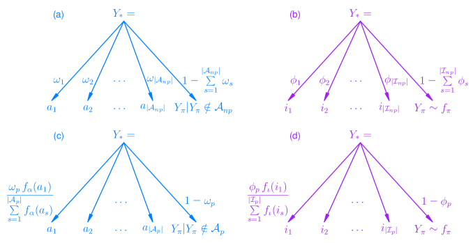
Figure 3: Decision tree diagram for generally-altered ((a), (c)) and generally-inflated ((b), (d)) distributions, abbreviated as (a) GA–$f_{\pi}$–MLM, (b) GI–$f_{\pi}$–MLM, (c) GA–$f_{\pi}$–$f_{\alpha}$, (d) GI–$f_{\pi}$–$f_{\iota}$, so that (a)–(b) are nonparametric and (c)–(d) are parametric. Here, $f_{\pi}$ is the parent distribution PMF, and $f_{\alpha}$ and $f_{\iota}$ are PMFs for the altered and inflated values. Also, $Y_{\pi}$ corresponds to the parent distribution and $Y_{*}$ is the response of interest. For (a)–(b) the positive probabilities $\omega_{s}$ and $\phi_{s}$ satisfy $0<\sum_{s=1}^{|\mbox{\scriptsize${\cal A}$}_{np}|}\omega_{s}<1$ and $0<\sum_{s=1}^{|\mbox{\scriptsize${\cal I}$}_{np}|}\phi_{s}<1$ and are modelled by an MLM. In (c) $\mbox{\rm Pr}(Y_{*}=a_{j})=\omega_{p}\,f_{\alpha}(a_{j})/{\sum_{s=1}^{|\mbox{\scriptsize${\cal A}$}_{p}|}f_{\alpha}(a_{s})}$; in (d) $\mbox{\rm Pr}(Y_{*}=i_{j})=\phi_{p}\,f_{\iota}(i_{j})/{\sum_{s=1}^{|\mbox{\scriptsize${\cal I}$}_{p}|}f_{\iota}(i_{s})}+(1-\phi_{p})\,f_{\pi}(i_{j})$.

1.3 Vector Generalized Linear Models

As GAITD regression is fitted as a VGLM via (14) they are briefly summarize here. Let the dimension of covariates $\mbox{$\bm{x}$}_{i}$ be $d$ with $x_{1}=1$ denoting the optional intercept. The log-likelihood is $\ell=\sum_{i=1}^{n}w_{i}^{*}\ell_{i}$ where the prior weights $w_{i}^{*}$ are positive, known and prespecified. VGLMs use multiple linear predictors $\eta_{j}$ to model multiple parameters.

For $M$ parameters $\theta_{j}$ VGLMs specify the $j$th linear predictor as

$$g_{j}(\theta_{j})~{}=~{}\eta_{j}~{}=~{}\mbox{\boldmath$\beta$}_{j}^{T}\mbox{$\bm{x}$}~{}=~{}\sum_{k=1}^{d}\;\beta_{(j)k}\,x_{k},~{}~{}~{}j=1,\ldots,M,$$ (1)

for some suitable parameter link function $g_{j}$ satisfying the usual properties. For example, the NBD as a VGLM has $\eta_{1}=\log\mu$ and $\eta_{2}=\log k$ by default. Since $M>1$ linear constraints between the regression coefficients are accommodated by

$$\mbox{\boldmath$\eta$}(\mbox{$\bm{x}$}_{i}) = \left(\eta_{1}(\mbox{$\bm{x}$}_{i}),\ldots,\eta_{M}(\mbox{$\bm{x}$}_{i})\right)^{T}~{}=~{}\sum_{k=1}^{d}\,\mbox{\boldmath$\beta$}_{(k)}\,x_{ik}~{}=~{}\sum_{k=1}^{d}\,\mbox{\rm\bf H}_{k}\,\mbox{\boldmath$\beta$}_{(k)}^{*}\,x_{ik}~{}=~{}\mbox{\rm\bf B}^{T}\mbox{$\bm{x}$}_{i},~{}~{}$$ (2)

for known constraint matrices $\mbox{\rm\bf H}_{k}$ of full column-rank (i.e., rank $R_{k}=$ ncol($\mbox{\rm\bf H}_{k}$)), and $\mbox{\boldmath$\beta$}_{(k)}^{*}$ is a possibly reduced set of regression coefficients to be estimated. While trivial constraints are denoted by $\mbox{\rm\bf H}_{k}=\mbox{\rm\bf I}_{M}$, other common examples include parallelism ($\mbox{\rm\bf H}_{k}={\bf 1}_{M}$), exchangeability, intercept-only parameters $\eta_{j}=\beta_{(j)1}^{*}$, and selecting different subsets of $\mbox{$\bm{x}$}_{i}$ for modelling each $\eta_{j}$. The overall ‘large’ model matrix is $\mbox{\rm\bf X}_{\mbox{\tiny VLM}}$, which is $\mbox{\rm\bf X}_{\mbox{\tiny LM}}\otimes\mbox{\rm\bf I}_{M}$ with trivial constraints, while $\mbox{\rm\bf X}_{\mbox{\tiny LM}}=[(x_{ik})]$ is the ‘smaller’ $n\times d$ model matrix associated with a $M=1$ model.

As with GLMs, iteratively reweighted least squares (IRLS)/Fisher scoring is the central algorithm for VGLMs. Consequently the score vector and expected information matrix (${\cal I}$_E; EIM) are needed (see the Supplementary Materials). In particular, let $\mbox{\rm\bf W}^{(a)}=(\mbox{\rm\bf W}_{1}^{(a)},\ldots,\mbox{\rm\bf W}_{n}^{(a)})$ be the working weight matrices, comprising $\mbox{\rm\bf W}_{i}^{(a)}=\mbox{}$ $-\mathrm{E}[\partial^{2}\ell_{i}/(\partial\mbox{\boldmath$\eta$}_{i}\,\partial\mbox{\boldmath$\eta$}_{i}^{T})]$ at iteration $a$. Fisher scoring has the $\mbox{\rm\bf W}_{i}$ as $\mbox{{\boldmath${\cal I}$}${}_{\mathrm{E},i}$}\circ\left[({\partial\mbox{\boldmath$\theta$}}/{\partial\mbox{\boldmath$\eta$}_{i}})({\partial\mbox{\boldmath$\theta$}^{T}}/{\partial\mbox{\boldmath$\eta$}_{i}^{T}})\right]$. That is,

$$(\mbox{\rm\bf W}_{i})_{uv} = -\mathrm{E}\left[\frac{\partial^{2}\ell_{i}}{\partial\eta_{u}\,\partial\eta_{v}}\right]~{}=~{}\mathrm{E}\left[\frac{-\partial^{2}\ell_{i}}{\partial\theta_{u}\,\partial\theta_{v}}\right]\;\frac{\partial\theta_{u}}{\partial\eta_{u}}\;\frac{\partial\theta_{v}}{\partial\eta_{v}}~{}=~{}(\mbox{{\boldmath${\cal I}$}${}_{\mathrm{E},i}$})_{uv}\cdot\left[\;g^{\prime}_{u}(\theta_{u})\;\,g^{\prime}_{v}(\theta_{v})\right]^{-1},~{}~{}~{}$$ (3)

say, for $u,v\in\{1,\ldots,M\}$. In particular, (3) holds for 1-parameter link functions $g_{u}$. The estimated variance-covariance matrix is $\widehat{\mbox{\rm Var}}\left(\widehat{\mbox{\boldmath$\beta$}^{*}}\right)=\left(\mbox{\rm\bf X}_{\mbox{\tiny VLM}}^{T}\;\widehat{\mbox{\rm\bf W}}\;\mbox{\rm\bf X}_{\mbox{\tiny VLM}}\right)^{-1}$ evaluated at the MLE, where $\mbox{\boldmath$\beta$}^{*}=(\mbox{\boldmath$\beta$}_{(1)}^{*T},\ldots,\mbox{\boldmath$\beta$}_{(d)}^{*T})^{T}$ are all the regression coefficients to be estimated.

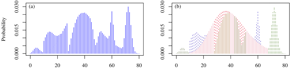
Figure 4: A GAITD–NB distribution with seven modes; (a) overall masked PMF; (b) PMF decomposed by the special values using color and various line types, e.g., the dip probabilities appear in reddish dashed lines.

2 The GAITD ‘Combo’ Model

2.1 Probability Mass Function

The (parametric and nonparametric) GAITD combo PMF is

$\mbox{\rm Pr}(Y_{*}=y;\mbox{\boldmath$\theta$}_{\pi},\omega_{p},\mbox{\boldmath$\theta$}_{\alpha},\phi_{p},\mbox{\boldmath$\theta$}_{\iota},\psi_{p},\mbox{\boldmath$\theta$}_{\delta},\mbox{\boldmath$\omega$}_{np},\mbox{\boldmath$\phi$}_{np},\mbox{\boldmath$\psi$}_{np})=f(y)=\mbox{}$

$$\left\{\begin{array}[]{ll}0,&y\in\mbox{${\cal T}$},\\ \omega_{p}\,{f_{\alpha}(y)}/{\sum\limits_{u\in\mbox{\scriptsize${\cal A}$}_{p}}f_{\alpha}(u)},{}{}{}{}{}&y\in\mbox{${\cal A}$}_{p},\\ \omega_{s},{}{}{}{}{}&y=a_{s}\in\mbox{${\cal A}$}_{np},\ s=1,\ldots,|{\mbox{${\cal A}$}_{np}}|,\\ \Delta\,f_{\pi}(y)+\phi_{p}\,f_{\iota}(y)/{\sum\limits_{u\in\mbox{\scriptsize${\cal I}$}_{p}}f_{\iota}(u)},{}{}{}{}{}&y\in\mbox{${\cal I}$}_{p},\\ \Delta\,f_{\pi}(y)+\phi_{s},{}{}{}{}{}&y=i_{s}\in\mbox{${\cal I}$}_{np},\ s=1,\ldots,|{\mbox{${\cal I}$}_{np}}|,\\ \Delta\,f_{\pi}(y)-\psi_{p}\,f_{\delta}(y)/\sum\limits_{u\in\mbox{\scriptsize${\cal D}$}_{p}}f_{\delta}(u),{}{}{}{}{}&y\in\mbox{${\cal D}$}_{p},\\ \Delta\,f_{\pi}(y)-\psi_{s},{}{}{}{}{}&y=d_{s}\in\mbox{${\cal D}$}_{np},\ s=1,\ldots,|{\mbox{${\cal D}$}_{np}}|,\\ \Delta\,f_{\pi}(y),&y\in\mbox{${\cal R}$}\backslash\mbox{${\cal S}$},\end{array}\right.$$ (12)

where the normalizing constant is

$$\Delta ~{}=~{} \frac{1-\omega_{p}-\phi_{p}+\psi_{p}-\sum\limits_{u=1}^{|\mbox{\scriptsize${\cal A}$}_{np}|}\omega_{u}-\sum\limits_{u=1}^{|\mbox{\scriptsize${\cal I}$}_{np}|}\phi_{u}+\sum\limits_{u=1}^{|\mbox{\scriptsize${\cal D}$}_{np}|}\psi_{u}}{1-\sum\limits_{a\in\{\mbox{\scriptsize${\cal A}$}_{p},\;\mbox{\scriptsize${\cal A}$}_{np}\}}f_{\pi}(a)-\sum\limits_{t\in\mbox{\scriptsize${\cal T}$}}f_{\pi}(t)}.$$ (13)

Alternatively, (12) might be called the complete or full GAITD model. It is fully specified
GA_pA_npI_pI_npD_pD_npT–$f_{\pi}(\mbox{${\cal R}$},\mbox{\boldmath$\theta$}_{\pi})$–$f_{\alpha}(\mbox{${\cal A}$}_{p},\omega_{p},\mbox{\boldmath$\theta$}_{\alpha})$–MLM($\mbox{${\cal A}$}_{np}$, $\mbox{\boldmath$\omega$}_{np}$)–$f_{\iota}(\mbox{${\cal I}$}_{p},\phi_{p},\mbox{\boldmath$\theta$}_{\iota})$–MLM($\mbox{${\cal I}$}_{np}$, $\mbox{\boldmath$\phi$}_{np}$)–$f_{\delta}(\mbox{${\cal D}$}_{p},\psi_{p},\mbox{\boldmath$\theta$}_{\delta})$–MLM($\mbox{${\cal D}$}_{np}$, $\mbox{\boldmath$\psi$}_{np}$)–${\cal T}$. The $\mbox{\boldmath$\theta$}_{\alpha}$ are asymptotically orthogonal to all the others.

Equation (12) has a simple structure. The term $\Delta\,f_{\pi}(y)$ is the scaled parent distribution from which the inflated and deflated values have probabilities added to or subtracted from to produce spikes or dips. In general, deflation can be thought of as the opposite of inflation. On $\mbox{${\cal A}$}_{np}$ the altered probabilities $\omega_{s}$ are ordinary probabilities estimated from the data which do not emanate from the scaled parent directly—Fig. 6(d) of a GAT-NB-MLM is an example. Elements from $\mbox{${\cal A}$}_{p}$ have a conditional $f_{\alpha}$ distribution on that subset.

Fig. 3 depicts flowcharts for four types of GA– and GI– submodels where plots (b) and (d) show the two-source concept for inflated values: (b) is nonparametric because the $\phi_{s}$ are unstructured while (d) is parametric because the additional probabilities are realizations from $f_{\iota}$ on a subset of its support. Plots (a) and (c) show how altered values only have a single source and repeat the same parametric versus nonparametric variant idea in GI submodels.

The precedence of the operators is truncation, alteration, inflation and lastly deflation, to avoid potential interference among them. Each line of (12) corresponds to a special value type except for the final line for the nonspecial values. It is clear that alteration occurs on a partitioned support whereas inflation and deflation occur on nested support. The parametric variants fit an additional distribution compared to the parent. The nonparametric variants entail estimating unstructured probabilities $\omega_{s}$, $\phi_{s}$ and $\psi_{s}$ as freely as possible using a MLM.

GAITD count distributions are exceedingly flexible, for example, they can accommodate up to seven modes, e.g., Fig. 4 uses a NB parent where the first plot is the overall distribution and the second unmasks each finite mixture by color and line type.

2.2 Goals and Inference

Based on (12), three fundamental questions that may be answered by GAITD regression are as follows. For concreteness, suppose age and sex are covariates.

1. For alteration, the probabilities exist in the usual form of an ordinary quantity $\omega_{s}$ or $\omega_{p}$, hence generally-altered regression explains why observations are there, e.g., which covariates explain $\mbox{\rm Pr}(Y=a_{s})$? How do age and sex affect $\mbox{\rm Pr}(Y=a_{s})$?

2. For inflation, the $\phi_{s}$ and $\phi_{p}$ are additions to the scaled parent distribution, hence may be called structural probabilities following $\phi$ being referred to as the probability of a structural 0 for the ZIP. Alternatively, the $\phi_{s}$ and $\phi_{p}$ may be called the excess (from extreme value terminology) or mixing probabilities. Generally-inflated regression accounts for why observations are there in excess, e.g., older males have a greater chance of being represented at certain values of $i_{s}$. What other variables contribute to overrepresentation at $i_{s}$?

3. For deflation, the $\psi_{s}$ and $\psi_{p}$ may be called dip probabilities because they are subtracted from the scaled parent distribution. Alternative names might be the shortfall or deficit probabilities. Generally-deflated regression explains why observations are not there, e.g., younger females may be underrepresented in the data at certain values of $d_{s}$.

Furthermore, while nonparametric GA–, GI– and GD– analysis at specific special values may be of interest in their own right, these analysis types may be used to deal with nuisance values—aberrant values that are not of interest but nevertheless must be adjusted for. (This is because the nonparametric variants model unstructured probabilities.) Hence the additional goals are:

1. nonparametric general-alteration may be used to ‘delete’ values equalling $a_{s}$ because some uninteresting probability $\omega_{s}$ is used to estimated it;

2. nonparametric general-inflation may be used to shave off the spikes so that inference may be directed at $f_{\pi}$;

3. nonparametric general-deflation may be used to fill in the dips (cracks or nonexisting values) so that inference may be focussed on $f_{\pi}$.

In short, nonparametric analyses disentangle various aberrations in the data to allow inference on the underlying parent distribution.

2.3 Multinomial Logit Model and Identifiability

The MLM for a probability $p_{s}$ has inverse link (softmax) of the form $e^{\eta_{s}}/\sum\limits_{m\in\mbox{\scriptsize${\cal M}$}}e^{\eta_{m}}$ for some set ${\cal M}$ and $\eta_{1+|\mbox{\scriptsize${\cal M}$}|}\equiv 0$ by default. (Further details are in the Supplementary Materials.) For 1-parameter distributions, the VGLM formulation (2) of (12) is $\mbox{\boldmath$\eta$}^{T}=\mbox{}$

$$\Bigg{(}g_{\pi}(\theta_{\pi}),~{}\log\frac{\omega_{p}}{\mbox{${\cal N}$}},~{}g_{\alpha}(\theta_{\alpha}),~{}\log\frac{\phi_{p}}{\mbox{${\cal N}$}},~{}g_{\iota}(\theta_{\iota}),~{}\log\frac{\psi_{p}}{\mbox{${\cal N}$}},~{}g_{\delta}(\theta_{\delta}),~{}\log\frac{\omega_{1}}{\mbox{${\cal N}$}},\ \ldots,~{}\log\frac{\omega_{|\mbox{\scriptsize${\cal A}$}_{np}|}}{\mbox{${\cal N}$}},~{}\qquad$$

$$~{}~{}~{}~{}~{}~{}\log\frac{\phi_{1}}{\mbox{${\cal N}$}},\ \ldots,~{}\log\frac{\phi_{|\mbox{\scriptsize${\cal I}$}_{np}|}}{\mbox{${\cal N}$}},~{}\log\frac{\psi_{1}}{\mbox{${\cal N}$}},\ \ldots,~{}\log\frac{\psi_{|\mbox{\scriptsize${\cal D}$}_{np}|}}{\mbox{${\cal N}$}}\Bigg{)}.~{}~{}~{}$$ (14)

where $\mbox{${\cal N}$}=1-\omega_{p}-\phi_{p}-\psi_{p}-\sum\limits_{u=1}^{|\mbox{\scriptsize${\cal A}$}_{np}|}\omega_{u}-\sum\limits_{u=1}^{|\mbox{\scriptsize${\cal I}$}_{np}|}\phi_{u}-\sum\limits_{u=1}^{|\mbox{\scriptsize${\cal D}$}_{np}|}\psi_{u}$ is the baseline probability. The ordering keeps the unstructured probabilities contiguous which simplifies the implementation. All but four linear predictors are coupled together by the MLM. The VGLM estimates all the parameters and probabilities by the regression coefficients in (2).

Disallowing degeneracy, the constraints on the parameter space needed for (12) to be identifiable are

$$\begin{array}[]{ll}0<\phi_{s}\mathrm{~{}for~{}}s=1,\ldots,|\mbox{${\cal I}$}_{np}|,{}{}{}{}{}{}&0<\phi_{p},\\ 0<\psi_{s}\mathrm{~{}for~{}}s=1,\ldots,|\mbox{${\cal D}$}_{np}|,{}{}{}{}{}{}&0<\psi_{p},\\ 0<\omega_{s}\mathrm{~{}for~{}}s=1,\ldots,|\mbox{${\cal A}$}_{np}|,&0<\omega_{p},{}{}{}{}{}{}\\[2.84544pt] \phi_{p}-\psi_{p}+\omega_{p}+\sum\limits_{s=1}^{|\mbox{\scriptsize${\cal I}$}_{np}|}\phi_{s}-\sum\limits_{s=1}^{|\mbox{\scriptsize${\cal D}$}_{np}|}\psi_{s}+\sum\limits_{s=1}^{|\mbox{\scriptsize${\cal A}$}_{np}|}\omega_{s}<1,{}{}{}{}&|\mbox{${\cal R}$}\backslash\mbox{${\cal S}$}|>0.\end{array}$$ (19)

The last condition ensures that the entire support cannot be inflated, deflated, altered or truncated, and guarantees that $\dim(\mbox{\boldmath$\theta$}_{\pi})\geq 1$; and if $\widetilde{\mbox{${\cal R}$}}$ is the support of the sample (i.e., set of all response values) then $|\widetilde{\mbox{${\cal R}$}}\backslash\mbox{${\cal S}$}|>0$ must hold too. Practically however, the number of nonspecial values should exceed unity to avoid a trivial regression. Note that $\omega_{p}=0$ is not permitted because otherwise $\mbox{${\cal A}$}_{p}$ could be subsumed into ${\cal T}$, and a similar argument holds for $\omega_{s}=0$, as well as for $\phi_{p}=0$, $\phi_{s}=0$, $\psi_{p}=0$ and $\psi_{s}=0$.

Continuing with identifiability issues, the ZAP can arise in two ways: either $\mbox{${\cal A}$}_{p}=\{0\}$ or $\mbox{${\cal A}$}_{np}=\{0\}$; and likewise $\mbox{${\cal I}$}_{p}=\{0\}$ or $\mbox{${\cal I}$}_{np}=\{0\}$ for the ZIP. To ensure the parameters are identifiable one can further enforce

$$|\mbox{${\cal A}$}_{p}|\neq 1,~{}~{}~{}~{}~{}|\mbox{${\cal I}$}_{p}|\neq 1\mathrm{~{}~{}and~{}~{}}|\mbox{${\cal D}$}_{p}|\neq 1.$$ (20)

3 GAITD Distributions: Properties & Applications

We present some basic distributional properties for the combo model and special cases.

3.1 Moments and CDF

For the combo mean and variance the $k$th moment is

$$\mathrm{E}[Y_{*}^{k}] = \frac{\omega_{p}\,\sum\limits_{a\in\mbox{\scriptsize${\cal A}$}_{p}}\,a^{k}\,f_{\alpha}(a)}{\sum\limits_{a\in\mbox{\scriptsize${\cal A}$}_{p}}\,f_{\alpha}(a)}+\frac{\phi_{p}\,\sum\limits_{i\in\mbox{\scriptsize${\cal I}$}_{p}}\,i^{k}\,f_{\iota}(i)}{\sum\limits_{i\in\mbox{\scriptsize${\cal I}$}_{p}}\,f_{\iota}(i)}-\frac{\psi_{p}\,\sum\limits_{d\in\mbox{\scriptsize${\cal D}$}_{p}}\,d^{k}\,f_{\delta}(d)}{\sum\limits_{d\in\mbox{\scriptsize${\cal D}$}_{p}}\,f_{\delta}(d)}+\sum\limits_{a\in\mathcal{A}_{np}}a^{k}\,\omega_{\lceil a\rceil}+\mbox{}$$

$$\sum\limits_{i\in\mathcal{I}_{np}}i^{k}\,\phi_{\lceil i\rceil}-\sum\limits_{d\in\mathcal{D}_{np}}d^{k}\,\psi_{\lceil d\rceil}+\Delta\cdot\left\{\mathrm{E}[Y_{\pi}^{k}]-\sum\limits_{t\in\mbox{\scriptsize${\cal T}$}}\,t^{k}\,f_{\pi}(t)-\sum\limits_{a\in\{\mbox{\scriptsize${\cal A}$}_{p},\;\mbox{\scriptsize${\cal A}$}_{np}\}}a^{k}\,f_{\pi}(a)\right\}.$$

Let $F_{*}$ be the GAITD cumulative distribution function (CDF) and $F_{\pi}$ the CDF of the parent distribution. Then

$$F_{*}(y) = \omega_{p}\;\frac{\sum\limits_{a\in\mathcal{A}_{p}}\mathrm{I}(a\leq y)\,f_{\alpha}(a)}{\sum\limits_{a\in\mbox{\scriptsize${\cal A}$}_{p}}\;f_{\alpha}(a)}+\phi_{p}\;\frac{\sum\limits_{i\in\mathcal{I}_{p}}\mathrm{I}(i\leq y)\,f_{\iota}(i)}{\sum\limits_{i\in\mbox{\scriptsize${\cal I}$}_{p}}\,f_{\iota}(i)}-\psi_{p}\;\frac{\sum\limits_{d\in\mathcal{D}_{p}}\mathrm{I}(d\leq y)\,f_{\delta}(d)}{\sum\limits_{d\in\mbox{\scriptsize${\cal D}$}_{p}}\,f_{\delta}(d)}+\mbox{}$$ (22)

$$\sum\limits_{a\in\mathcal{A}_{np}}\;\mathrm{I}(a\leq y)\,\omega_{\lceil a\rceil}+\sum\limits_{i\in\mathcal{I}_{np}}\;\mathrm{I}(i\leq y)\,\phi_{\lceil i\rceil}-\sum\limits_{d\in\mathcal{D}_{np}}\;\mathrm{I}(d\leq y)\,\psi_{\lceil d\rceil}+\mbox{}$$

$$\Delta\cdot\left\{F_{\pi}(y)-\sum\limits_{t\in\mathcal{T}}\;\mathrm{I}(t\leq y)\,f_{\pi}(t)-\sum\limits_{a\in\{\mathcal{A}_{p},\,\mathcal{A}_{np}\}}\;\mathrm{I}(a\leq y)\,f_{\pi}(a)\right\}.$$

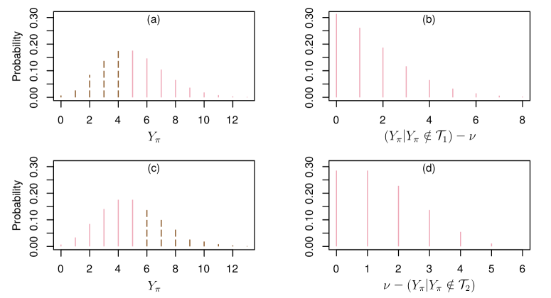
Figure 5: Two generally-truncated Poisson distributions with amount of shift $\nu=5$. The parent PMF $f_{\pi}$ is for $Y_{\pi}\sim\mathrm{Pois}(\lambda_{\pi}=5)$. (a) $f_{\pi}$ with $\mbox{${\cal T}$}_{1}=\{0,1,2,3,4\}$ is dashed, (b) $Y_{*}=Y_{\pi}-\nu\sim$ GT–$f_{\pi}$–$\mbox{${\cal T}$}_{1}$ matches the upper tail, (c) $f_{\pi}$ with $\mbox{${\cal T}$}_{2}=\{6,7,\ldots\}$ dashed, (d) $Y_{*}=\nu-Y_{\pi}\sim$ GT–$f_{\pi}$–$\mbox{${\cal T}$}_{2}$ matches the lower tail. Tan dashed lines have been truncated, and the pink solid lines are used for $Y_{*}$.

3.2 Two Measures: Kullback–Leibler Divergence and $\Xi$

A natural question is: how can the total effect of alteration, inflation, truncation and deflation be measured relative to the parent distribution? Because its formula allows simplification, a convenient solution is to compute a divergence measure such as the Kullback–Leibler divergence (KLD) (Kullback and Leibler, 1951). Denoting the PMFs by $f(\cdot)$ and $f_{\pi}(\cdot)$, $D_{\mathrm{KL}}(f\ \|\ f_{\pi})=\mbox{}$

$$\omega_{p}\left[\log\frac{\omega_{p}}{{\sum\limits_{u\in\mbox{\scriptsize${\cal A}$}_{p}}f_{\alpha}(u)}}+\sum\limits_{a\in\mbox{\scriptsize${\cal A}$}_{p}}\,A_{\alpha}(a)\;\log\frac{f_{\alpha}(a)}{f_{\pi}(a)}\right]+\sum\limits_{s=1}^{|\mbox{\scriptsize${\cal A}$}_{np}|}\omega_{s}\,\log\frac{\omega_{s}}{f_{\pi}(a)}+\Delta\,\left(\log\Delta\right)\;\mbox{\rm Pr}(y\notin\mbox{${\cal S}$})+\mbox{}~{}~{}~{}~{}$$

$$\sum\limits_{i\in\mbox{\scriptsize${\cal I}$}_{p}}\left[\Delta\,f_{\pi}(i)+\phi_{p}\,A_{\iota}(i)\right]\;\log\left\{\Delta+\phi_{p}\,\frac{A_{\iota}(i)}{f_{\pi}(i)}\right\}+\sum\limits_{s=1}^{|\mbox{\scriptsize${\cal I}$}_{np}|}\left[\Delta\,f_{\pi}(i_{s})+\phi_{s}\right]\;\log\left\{\Delta+\frac{\phi_{s}}{f_{\pi}(i_{s})}\right\}+\mbox{}$$

$$\sum\limits_{d\in\mbox{\scriptsize${\cal D}$}_{p}}\left[\Delta\,f_{\pi}(d)-\psi_{p}\,A_{\delta}(d)\right]\;\log\left\{\Delta-\psi_{p}\,\frac{A_{\delta}(d)}{f_{\pi}(d)}\right\}+\sum\limits_{s=1}^{|\mbox{\scriptsize${\cal D}$}_{np}|}\left[\Delta\,f_{\pi}(d_{s})-\psi_{s}\right]\;\log\left\{\Delta-\frac{\psi_{s}}{f_{\pi}(d_{s})}\right\}~{}~{}~{}~{}$$ (23)

as $0\cdot\log 0\equiv 0$ by a limit argument, where $\mbox{\rm Pr}(y\notin\mbox{${\cal S}$})=1-\omega_{p}-\phi_{p}-\psi_{p}-\sum_{t\in\mbox{\scriptsize${\cal T}$}}f_{\pi}(t)-\sum_{u=1}^{|\mbox{\scriptsize${\cal A}$}_{np}|}\omega_{u}-\sum_{u=1}^{|\mbox{\scriptsize${\cal I}$}_{np}|}\phi_{u}-\sum_{u=1}^{|\mbox{\scriptsize${\cal D}$}_{np}|}\psi_{u},$ and $A_{\alpha}(y)={f_{\alpha}(y)}/{\sum\limits_{u\in\mbox{\scriptsize${\cal A}$}_{p}}f_{\alpha}(u)}$, $A_{\iota}(y)={f_{\iota}(y)}/{\sum\limits_{u\in\mbox{\scriptsize${\cal I}$}_{p}}f_{\iota}(u)}$, etc.

Rather than using the KLD, a related question is: what proportion of the data is heaped or seeped? It is proposed that the approximate measure $\Xi:=\mbox{}$

$$\sum\limits_{a\in\mbox{\scriptsize${\cal A}$}_{p}}\left|\Delta f_{\pi}(a)-\frac{\omega_{p}\,f_{\alpha}(a)}{\sum\limits_{u\in\mbox{\scriptsize${\cal A}$}_{p}}\;f_{\alpha}(u)}\right|+\sum\limits_{s=1}^{|\mbox{\scriptsize${\cal A}$}_{np}|}\bigg{|}\Delta f_{\pi}(a_{s})-\omega_{s}\bigg{|}+\max\!\left(\phi_{p}+\sum\limits_{s=1}^{|\mbox{\scriptsize${\cal I}$}_{np}|}\phi_{s},~{}\psi_{p}+\sum\limits_{s=1}^{|\mbox{\scriptsize${\cal D}$}_{np}|}\psi_{s}\right)~{}~{}$$ (24)

based on (12)–(13) be used which measures the discrepancy between the GAITD PMF and the scaled parent distribution on $\mbox{${\cal S}$}\backslash\mbox{${\cal T}$}$. Being opposites, the maximum of total inflation and deflation is taken.

3.3 GT–Expansion Method for Underdispersed Data

Even armed with the flexibility afforded by general truncation alone, the following is the first of two useful GAITD special cases.

Intuitively, the Generally-Truncated–Expansion (GTE) method combats underdispersion by a count-preserving transformation that increases the spread at a greater rate than the mean. This is achieved by simply multiplying the response by some integer $m\ (>1)$ and generally-truncating the values in between, e.g., doubling $Y$ and truncating odd values. By choosing integer $m$, the expanded response remains integer-valued. Writing $Y\sim(\mu,\ \sigma^{2})$ for the first moments, then $mY\sim(m\mu,\ m^{2}\sigma^{2})$ has a variance-to-mean ratio (VMR or dispersion index) of $m\sigma^{2}/\mu$. Since $\sigma^{2}/\mu<1$ for underdispersed data, there exists sufficiently large $m$ whereby the VMR $\geq 1$. Ideally the aim is to transform $Y$ to equidispersion, or near equidispersion if possible, and apply the GAITD–Poisson. If not, then transform to mild to moderate overdispersion and use the GAITD–NB. As the expansion factor $m$ is not unique, it is suggested that the smallest value achieving equidispersion or overdispersion be used. Further motivation for the GTE method derives from there being more distributions for handling overdispersion compared to underdispersion (Sellers and Morris, 2017).

Expressing this more formally, consider an inverse location–scale transformation

$$Y_{**}~{}=~{}\nu+mY_{*},\ \ \ ~{}m\in\mathbb{Z}^{+},\ \ ~{}\nu\in\mathbb{Z},$$ (25)

where usually the multiplier $m>1$ is small and $\nu$ nonnegative. The distribution has its support shifted to the right by $\nu$ after being expanded and separated by $m$, hence by generally-truncating the values in between, underdispersion can be handled. If $\nu=0$ then $Y_{**}\sim$ GT–$f_{\pi}(\mbox{\boldmath$\theta$}_{\pi})$ with $\mbox{${\cal T}$}=\mathbb{Z}^{+}\,\backslash\,\{m,2m,\ldots\}$. Values for $m$ and $\nu$ may be known or estimated. As an example, using the Poisson as $f_{\pi}$, if $\nu=0$ then the sample variance and mean are $m^{2}s_{y_{*}}^{2}$ and $m\overline{y_{*}}$, hence yields the moment estimator

$$\widehat{m} = {\overline{y_{*}}}/{s_{y_{*}}^{2}}.$$ (26)

In practice one would round this and/or choose an integer $>\widehat{m}$. The method suggests that if the dispersion index $\in(\frac{2}{3},1)$ then the amount of underdispersion is too slight to require adjustment to equidispersion. When fitting the VGLM a $\log m$ offset is needed because $\log\mu_{**}=\log(m\mu_{*})$. The method is illustrated by handling counts undispersed relative to the Poisson in Section 6.1.

3.4 GT for Contiguous Segments

A second useful GAITD special case is based on the ability of general-truncation to allow selection of any single contiguous segment of a parent distribution’s PMF to be fitted to data. It is (25) with $m=\pm 1$ and $\nu\in\mathbb{Z}$. For example, Fig. 5(a)–(b) shows the upper tail of a Poisson$(\lambda_{\pi}=5)$ being used by having $\mbox{${\cal T}$}_{1}=\{0,1,\ldots,\nu-1\}$ for $\nu=5$ so that $Y_{*}+\nu\sim$ GT–Pois($\lambda_{\pi};\ \mbox{${\cal T}$}_{1}=\{0,1,\ldots,\nu-1\}$). That is, the RHS of a Poisson distribution is selected to be the complete distribution (after appropriate scaling) of a right-skewed data set.

In the Fig. 5(c)–(d) example a reflection is used: $\nu-Y_{*}\sim$ GT–Pois($\lambda_{\pi};\ \mbox{${\cal T}$}_{2}=\{\nu+1,\nu+2,\ldots\}$) where $\nu=5$. That is, the LHS of a Poisson distribution is selected to be the complete distribution of an upper-truncated data set that happens to have a rough half-normal shape.

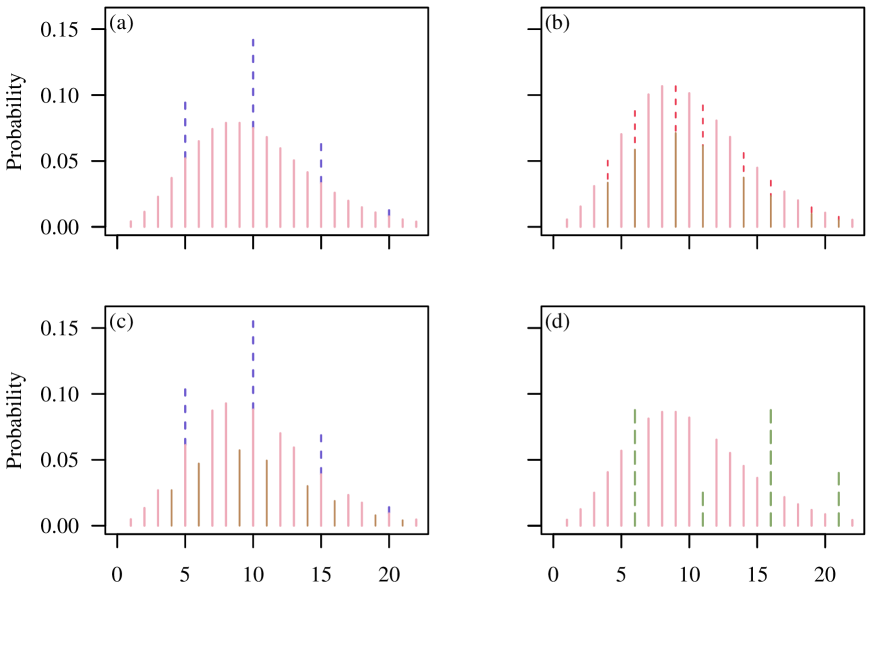
Figure 6: Heaped and/or seeped data—idealized forms in (a)–(c). The NBD is the parent. The special values are $\mbox{${\cal I}$}_{p}=\{5,10,15,20\}$, $\mbox{${\cal D}$}_{p}=\{4,6,9,11,14,16,19,21\}$, $\mbox{${\cal T}$}=\{0\}$, with $\omega_{p}=\psi_{p}=0.15$, $\mu_{\pi}=k_{\pi}=10$ so that $f_{\pi}=f_{\iota}=f_{\delta}$ are the NB(10, 10) PMF. (a) GIT–NB–NB; (b) GTD–NB–NB with the dip probabilities shown; (c) GITD-NB-NB-NB combines them together; (d) GAT-NB-MLM($\mbox{\boldmath$\omega$}_{np}=(0.09,0.03,0.09,0.04)^{T}$). The parent distribution comprises the pink solid lines, the excess probabilities are indigo dashed spikes, the dip probabilities are reddish dashed lines, and the altered probabilities are artichoke-colored dashed lines.

3.5 Heaped and Seeped Data

Figure 6(a)–(c) illustrates heaping and seeping based on a NB parent, where all plots have $\mbox{${\cal T}$}=\{0\}$. Inflation occurs at multiples of 5 and are shown by dashed indigo lines appearing as spikes in (a). Deflation occurs at the nearest surrounding values in (b) where the dip probabilities are the dashed lines. The combined plot (c) is the idealized heaping-and-seeping scenario because the deficit probabilities are morphed into excess probabilities. Somewhat unrelated, plot (d) illustrates a GAT-NB-MLM where the dashed artichoke-coloured lines lie arbitrarily below or above the scaled $f_{\pi}$.

In contrast to excesses in Fig. 6(a), we describe the deficits in Fig. 6(b) as due to seeped data because some of the nominal parent probabilities have oozed out, so to speak, due to measurement error. Strictly speaking, it may be argued that heaping and seeping form an if-and-only-if relationship: they appear together or not at all because spikes must come from dips, and vice versa. Because there is a conservation of probabilities such as $\phi_{\lceil i\rceil}=\psi_{\lceil i-1\rceil}+\psi_{\lceil i+1\rceil}$ for an inflated value $i$, modelling them ideally requires the same variant, i.e., $\mbox{${\cal I}$}_{p}$ and $\mbox{${\cal D}$}_{p}$, else $\mbox{${\cal I}$}_{np}$ and $\mbox{${\cal D}$}_{np}$. However, in practice, it would be too strong an assumption to expect this for all $i$ in a given data set. As mentioned in Section 1.1 the adjacency holds at $i=30$ years in Fig. 2, however it does not appear to hold at $i=25$ or 35.

There is now a sizeable literature on heaped data occurrence. Crawford et al. (2015) mention a wide range of examples taken from self-reported smoking rates, duration of breastfeeding, household total expenditure, number of drug partners and age at menopause. Not adjusting for heaping in regression can result in biased estimation (Wang and Heitjan, 2008). In other situations heaping may lead to underestimation of within-subject variability (Wang et al., 2012). Despite Crawford et al. (2015, p.572) stating that “inference for heaped data is an important statistical problem” we opine that most techniques proposed have been unduly complex and indeed, among the c.18,500 R packages currently on CRAN, there appears only one directly focussed on heaped data (Kernelheaping). In contrast, we believe that GAITD regression is more accessible and flexible than competing methods.

3.6 Special Cases

We take the opportunity to comment on some special cases. The GA–$f_{\pi}$–MLM and GA–$f_{\pi}$–$f_{\alpha}$ are a (discrete) spliced or composite distribution since the mixture components form the partition $\mbox{${\cal A}$}_{p}\cup(\mbox{${\cal R}$}\backslash\mbox{${\cal A}$}_{p})$ of ${\cal R}$. In contrast, GI–$f_{\pi}$–MLM and GI–$f_{\pi}$–$f_{\iota}$ are not strictly spliced distributions because their component supports are $\mbox{${\cal I}$}_{p}$ and ${\cal R}$ with the former nested within the latter (Su et al. (2013) propose a GI-like model). In a comprehensive review of mixed Poisson distributions (Karlis and Xekalaki, 2005) the idea of a spliced or partially spliced distribution is not mentioned among the many members cited. To the best of our knowledge GAITD regression comprising interlacing discrete spliced and partially spliced distributions is novel.

One can easily constrain $\mbox{\boldmath$\theta$}_{\pi}=\mbox{\boldmath$\theta$}_{\alpha}$ and $\mbox{\boldmath$\theta$}_{\pi}=\mbox{\boldmath$\theta$}_{\iota}$ in both GAT–$f_{\pi}$–$f_{\alpha}$ and GIT–$f_{\pi}$–$f_{\iota}$ models using the constraint matrices of (2). As a simple example, for GAT–Pois($\lambda_{\pi}$)–Pois-($\lambda_{\alpha}$) the constraint $\lambda_{\pi}=\lambda_{\alpha}$ can be enforced by

$$\mbox{\rm\bf H}_{k}=\left(\begin{array}[]{ccc}1&0&1\\ 0&1&0\end{array}\right)^{T},\qquad k=1,\ldots,d,$$

in (2) because $\mbox{\boldmath$\eta$}=(\log\,\lambda_{\pi},\ \mbox{\rm logit}\,\omega_{p},\ \log\,\lambda_{\alpha})^{T}$ if $|\mbox{${\cal A}$}_{p}|>1$. The software easily allows this. A likelihood ratio test is valid for formally testing for equal rate parameters.

4 Joint Under– and Over-dispersion Analysis

The separate effects of 0-alteration, 0-inflation, and 0-truncation on overdispersion in Poisson regression has been considered by a number of authors, e.g., Ridout et al. (2001), Tang et al. (2015), Sellers and Raim (2016) and Haslett et al. (2022), however GAITD distributions allow a more general and joint investigation of this phenomenon from the four operators. Indeed, there is an almost plethora of possibilities. It is found more convenient to use the variance-to-mean difference (VMD) $\mbox{\rm Var}\,Y-\mathrm{E}\,Y$ rather than the VMR. Determining overdispersion is exacerbated by having at least two possible definitions, with both having their merits:

$$\mathrm{VMD}_{*}:\quad \mbox{\rm Var}\,Y_{*}-\mathrm{E}\,Y_{*}~{}>~{}0,$$ (27)

$$\mathrm{VMD}_{\pi}:\quad \mbox{\rm Var}\,Y_{*}-\mathrm{E}\,Y_{\pi}~{}>~{}0.$$ (28)

The former transfers the VMD comparison onto the new distribution while the latter compares the variance of the modified distribution to parent mean. They primarily are only applicable to the Poisson, hence more generally define the variance-to-variance difference as

$$\mathrm{VVD}:\quad \mbox{\rm Var}\,Y_{*}-\mbox{\rm Var}\,Y_{\pi}~{}>~{}0$$ (29)

to replace (28). This compares the variances of the modified and parent distributions and can be applied to distributions such as the binomial (the VMD_π and VVD coincide for the Poisson.)

Alternatively to the above perhaps it is better to quantify overdispersion more symmetrically based on both pairs of the first two moments:

$$\mathrm{DVMD} = \mbox{\rm Var}\,Y_{*}-\mathrm{E}\,Y_{*}-\left(\mbox{\rm Var}\,Y_{\pi}-\mathrm{E}\,Y_{\pi}\right)~{}>~{}0,$$ (30)

$$\mathrm{DIR} = \frac{\mbox{\rm Var}\,Y_{*}/\mathrm{E}\,Y_{*}}{\mbox{\rm Var}\,Y_{\pi}/\mathrm{E}\,Y_{\pi}}~{}>~{}1,$$ (31)

where the acronyms are self-explanatory. For the Poisson the VMD_∗ and DVMD coincide, as does the DIR and VMD_π because the denominator is unity.

Possibly the most tractable method for studying overdispersion in Poisson regression while allowing for the joint effects of the four operators is the following result.

Theorem  (i) Under the VMD_∗ (27), overdispersion relative to the Poisson distribution will occur for the GAITD–$f_{\pi}$–$f_{\alpha}$–MLM–$f_{\iota}$–MLM–$f_{\delta}$–MLM combo if

$$\frac{\omega_{p}\,\sum\limits_{a\in\mbox{\scriptsize${\cal A}$}_{p}}\,a(a-1)\,f_{\alpha}(a)}{\sum\limits_{a\in\mbox{\scriptsize${\cal A}$}_{p}}\,f_{\alpha}(a)}+\frac{\phi_{p}\,\sum\limits_{i\in\mbox{\scriptsize${\cal I}$}_{p}}\,i(i-1)\,f_{\iota}(i)}{\sum\limits_{i\in\mbox{\scriptsize${\cal I}$}_{p}}\,f_{\iota}(i)}-\frac{\psi_{p}\,\sum\limits_{d\in\mbox{\scriptsize${\cal D}$}_{p}}\,d(d-1)\,f_{\delta}(d)}{\sum\limits_{d\in\mbox{\scriptsize${\cal D}$}_{p}}\,f_{\delta}(d)}+\mbox{}$$

$$\sum_{a\in\mbox{\scriptsize${\cal A}$}_{np}}\,a(a-1)\,\omega_{\lceil a\rceil}+\sum_{i\in\mbox{\scriptsize${\cal I}$}_{np}}\,i(i-1)\,\phi_{\lceil i\rceil}-\sum_{d\in\mbox{\scriptsize${\cal D}$}_{np}}\,d(d-1)\,\psi_{\lceil d\rceil}+\mbox{}$$ (32)

$$\Delta\;\cdot\left\{\mathrm{E}[Y_{\pi}(Y_{\pi}-1)]-\sum\limits_{a\in\{\mbox{\scriptsize${\cal A}$}_{p},\;\mbox{\scriptsize${\cal A}$}_{np}\}}\,a(a-1)\,f_{\pi}(a)-\sum\limits_{t\in\mbox{\scriptsize${\cal T}$}}\,t(t-1)\,f_{\pi}(t)\right\}~{}>~{}\mu_{*}^{2},$$

where $\mu_{*}$ is given by (3.1) with $k=1$; (ii) Likewise, under the VMD_π (28) if

$$\frac{\omega_{p}\,\sum\limits_{a\in\mbox{\scriptsize${\cal A}$}_{p}}\,(a-\mu_{*})^{2}\,f_{\alpha}(a)}{\sum\limits_{a\in\mbox{\scriptsize${\cal A}$}_{p}}\,f_{\alpha}(a)}+\frac{\phi_{p}\,\sum\limits_{i\in\mbox{\scriptsize${\cal I}$}_{p}}\,(i-\mu_{*})^{2}\,f_{\iota}(i)}{\sum\limits_{i\in\mbox{\scriptsize${\cal I}$}_{p}}\,f_{\iota}(i)}-\frac{\psi_{p}\,\sum\limits_{d\in\mbox{\scriptsize${\cal D}$}_{p}}\,(d-\mu_{*})^{2}\,f_{\delta}(d)}{\sum\limits_{d\in\mbox{\scriptsize${\cal D}$}_{p}}\,f_{\delta}(d)}+\mbox{}$$

$$\sum_{a\in\mbox{\scriptsize${\cal A}$}_{np}}\,(a-\mu_{*})^{2}\,\omega_{\lceil a\rceil}+\sum_{i\in\mbox{\scriptsize${\cal I}$}_{np}}\,(i-\mu_{*})^{2}\,\phi_{\lceil i\rceil}-\sum_{d\in\mbox{\scriptsize${\cal D}$}_{np}}\,(d-\mu_{*})^{2}\,\psi_{\lceil d\rceil}+\mbox{}$$ (33)

$$\Delta\;\cdot\left\{\sigma_{\pi}^{2}+(\mu_{\pi}-\mu_{*})^{2}-\sum\limits_{a\in\{\mbox{\scriptsize${\cal A}$}_{p},\;\mbox{\scriptsize${\cal A}$}_{np}\}}\,(a-\mu_{*})^{2}\,f_{\pi}(a)-\sum\limits_{t\in\mbox{\scriptsize${\cal T}$}}\,(t-\mu_{*})^{2}\,f_{\pi}(t)\right\}~{}>~{}\mu_{\pi};~{}~{}~{}$$

(iii) Likewise, under the VVD (29), if (33) but with $\sigma_{\pi}^{2}=\mbox{\rm Var}\,Y_{\pi}$ replacing $\mu_{\pi}$ on the RHS.

Proof  Overdispersion for VMD_∗ follows from $\mathrm{E}[Y_{*}(Y_{*}-1)]>\{\mathrm{E}(Y_{*})\}^{2}$. The other cases are straightforward and use $\mathrm{E}\left[\left(Y_{\pi}-\mu_{*}\right)^{2}\right]=\mbox{\rm Var}(Y_{\pi})+(\mu_{\pi}-\mu_{*})^{2}$. $\Box$

Corollary  For nondegenerate 0-altered count distributions overdispersion with respect to VMD_∗ occurs when

$$\frac{1-\omega}{1-f_{\pi}(0)}\left[\,\sigma_{\pi}^{2}-\mu_{\pi}+\frac{\mu_{\pi}^{2}\,\{\omega-f_{\pi}(0)\}}{1-f_{\pi}(0)}\right]~{}>~{}0.$$ (34)

So for the Poisson distribution overdispersion occurs when $\mbox{\rm Pr}(Y_{\pi}=0)<\omega$, i.e., 0 is heaped, and underdispersion when 0 is seeped.

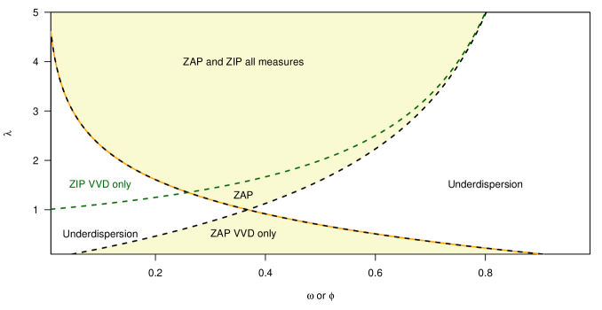
Figure 7: Regions in the parameter space where ZA- and ZI-Poisson($\lambda_{\pi}$) regressions are overdispersed relative to the Poisson, according to definitions (27)–(31). Approximately, the parameter space is $\lambda_{\pi}\in(0.1,5)$ and $\omega$ and $\phi\in(0,1)$. The ZAP VVD is shaded.

According to the various definitions, it is interesting to see the conditions for which overdispersion occurs for two common 1-parameter count distributions with 0 as the special value. Table 1 is a summary of the Poisson and binomial cases. Several points emerge, e.g.,

• the different definitions do yield different conditions for overdispersion. Zero-truncation does not result in overdispersion by any measure.

• The VVD tends to produce the most complicated conditions because overdispersion occurs in two disjoint regions of the parameter space. However, overdispersion does not occur for the ZAP when $\lambda=1$ and $\omega=e^{-1}$, nor does it occur for the ZAB when $p=1/(N+1)$ and $\omega=(1-p)^{N}$; in these cases equidispersion occurs.

• Zero-inflation tends to result in overdispersion more than alteration.

• Zero-alteration usually occurs when $\omega$ is too large, which contrasts with zero-inflation which usually occurs when $\phi$ is too small.

Fig. 7 displays partitions the parameter space for the Poisson parent with $0.1<\lambda_{\pi}<5$ and $0<\omega/\phi<1$. Overdispersion occurs in regions above the curves, and in the case of the ZAP-VVD it also occurs in the region wedged in at the central bottom. Excluding zero-truncation, overdispersion tends to increase with increasing $\lambda_{\pi}$ because the distribution shifts away from the origin to leave the point mass at 0 for creating extra variation.

Table 1: Summary of conditions for overdispersion under definitions (27)–(31): the 0-altered, 0-inflated and 0-truncated cases are considered for the Poisson and binomial parent distributions where $0<\lambda<\infty$, $0<p<1$, $0<\omega<1$ and $0<\phi<1$ are assumed. Here, $q=1-p$, $\phi=\mbox{\rm Pr}(Y=0)$ structurally and $\omega=\mbox{\rm Pr}(Y=0)$; and $\dagger$ indicates the endpoints of the interval may need switching to preserve the order.

$f$	VMD∗	VVD	DVMD	DIR
ZAP($\lambda,\ \omega$)	$e^{-\lambda}<\omega$	$\omega\in\displaystyle{\left[e^{-\lambda},\ 1-\frac{1-e^{-\lambda}}{\lambda}\right]}\,\dagger~{}~{}$	$e^{-\lambda}<\omega$	$e^{-\lambda}<\omega$
ZAB($N,\ p,\ \omega$)	$q^{N}+\displaystyle{\frac{1-q^{N}}{N}<\omega}$	$\omega\in\displaystyle{\left[q^{N},\ 1-\frac{q(1-q^{N})}{N(1-q)}\right]}\,\dagger~{}$	$\displaystyle{q^{N}<\omega}$	$q^{N}<\omega$
ZIP($\lambda,\ \phi$)	Always	$\phi<\displaystyle{1-\frac{1}{\lambda}}$	Always	Always
ZIB($N,\ p,\ \phi$)	Always	$\phi<1-\displaystyle{\frac{1-p}{Np}}$	Always	Always
ZTP($\lambda$)	Never	Never	Never	Never
ZTB($N,\ p$)	Never	Never	Never	Never

5 Maximum Likelihood Estimation

The technical details and derivative systems for maximizing $\ell$ by Fisher scoring/IRLS are given in the Supplementary Materials; here we give commentary on a few overarching details.

The full parameter space for GAITD regression is described by the last equations of (12) and (19) coupled with (13). Since $\Delta>0$ implies

$$0~{}<~{}\omega_{p}+\phi_{p}+\sum\limits_{u=1}^{|\mbox{\scriptsize${\cal A}$}_{np}|}\omega_{u}+\sum\limits_{u=1}^{|\mbox{\scriptsize${\cal I}$}_{np}|}\phi_{u}~{}<~{}1+\psi_{p}+\sum\limits_{u=1}^{|\mbox{\scriptsize${\cal D}$}_{np}|}\psi_{u},$$

it is seen that the parameter space boundary is not fixed, hence this dependency breaches a standard regularity condition. A consequence is that $\mathrm{E}[\partial\ell/\partial\psi_{p}]=2\neq 0$ for example. Instead, we estimate the probabilities in (14) by an ordinary MLM. Operating in a reduced parameter space may occasionally create inconvenience because the probability of the baseline reference group, $\mbox{\rm Pr}(y\notin\mbox{${\cal S}$})$, may become perilously close to 0, e.g., when there is much nonparametric inflation or deflation so that the sum of the $\phi_{s}$ and $\psi_{s}$ is large. In contrast, it would have been ideal if deflation could release probability back into the model that could be used for inflation, however this is not possible. Using the MLM to estimate the model means that the parameter space used is $1/[1+2\phi_{p}+2\sum\psi_{v}]$ the size of the ‘proper’ parameter space. We call $\mbox{\rm Pr}(y\notin\mbox{${\cal S}$})$ the nonspecial baseline probability (NBP) or reserve probability. Because it must be positive it pays to be specify the $\psi_{s}$ economically so that one does not exhaust the reserve probability unnecessarily.

There will be the occasional dataset exhibiting much inflation and deflation. The following strategies can help economize the probability-consumption problem caused by MLM estimation.

1. Parametric inflation/deflation is more economical; can some $\phi_{s}$/$\psi_{s}$ be represented by $\phi_{p}$/$\psi_{p}$? For example, $\psi_{s}\equiv\psi_{p}\,f_{\delta}(y)$.

2. If $\psi_{s}>\frac{1}{2}f_{\pi}(y)$ then use $\omega_{s}$ instead, i.e., alter $y$ rather than deflating it.

6 Examples

Data for both examples are subsets from a large ($n=10,529$) New Zealand cross-sectional study (and an approximate random sample of the country’s working population then) collected in the mid-1990s (MacMahon et al., 1995). Code for reproducing the analyses are included in the Supplementary Materials.

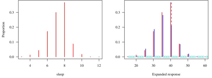
Figure 8: (a) Spikeplot of sleep in xs.nz from VGAMdata; (b) GT-Expansion method with GIT-Poisson fit is overlaid adjacently in blue—the truncated values are turquoise hollow points.

6.1 Sleep Duration

To simply illustrate the GT-Expansion method we consider the self-reported sleep duration response to the question “How many hours do you usually sleep each night?” All recorded answers were integer-valued, and after removing the missing values and outliers ($2.4\%$) there were $n=10,264$ individuals; specifically, $y\in\{3,\ldots,12\}$ so we chose $\mbox{${\cal T}$}=\{0,1,2,13,14,\ldots\}$ to account for the removals and physical limits.

The data (Table 2) comprises of 10 values and might be considered only marginally heaped because there are no obvious spikes even though the data are clearly tainted by measurement error. A routine Poisson regression is not amenable because: (i) there is strong underdispersion (the sample mean and variance are $7.3$ and $1.3$); (ii) left-skew is apparent (Fig. 8(a)) while the Poisson tends to be right-skewed. We combat these by applying the GTE method and assigning $\mbox{${\cal I}$}_{np}=\{8\}$. The 8-inflation might be justified because of the common belief that about 8 hours sleep is recommended for most adults (e.g., Hirshkowitz et al., 2015).

Table 2: Usual sleep duration in a New Zealand cross-sectional data.

Hours	3	4	5	6	7	8	9	10	11	12
Frequency	16	125	443	1760	3076	3766	891	170	10	7

A simple search over all multipliers yields $m=5$ for maximizing the GIT likelihood. This compares to the moment estimator (26) which is $5.67$. Fig. 8(b) overlays the GIT model on the data and a good fit to the observed proportions is seen. The model indicates that the amount of inflation is $\widehat{\phi}_{\lceil 8\rceil}\approx 0.157$—almost 1/6 of the entire data set. The Kullback-Leibler divergence from the model to an ordinary Poisson is $4.57$. The overall GIT mean, (3.1), is estimated by $7.297$ hours whereas an approximate 95% confidence interval for $\mu_{\pi}$ is $[7.139,7.194]$ hours. The former is higher because the 8-inflation draws the overall mean towards it.

6.2 Smoking Duration

This example concerns how long current smokers or ex-smokers reported smoking in years. A small fraction of the data (about $0.2$%) had values 0.1, 0.2, 0.3 and 0.5 which were rounded, as well as $2.5$% that were missing values and were deleted. The positive integer-valued smoking duration data set has $n=5492$ with almost half having never smoked (about $48$%). Of those who do, Fig. 2 shows a heavy-tailed distribution of smoking duration with one or two layers of heaping that is unimodal with mean between 10 and 20 years. The most pronounced heaped values include $\mbox{${\cal I}$}_{p}=\{5,10,20,30,40,50,60\}$, as well as 12, 25, 35. A careful examination also suggests that $\mbox{${\cal D}$}_{p}=\{9,11,13,19,21,29,31\}$ are seeped. Furthermore, we chose $\mbox{${\cal A}$}_{p}=\{2,15,25,35,45\}$, $\mbox{${\cal I}$}_{np}=\{1,8,12,18\}$, and a NB parent to handle overdispersion. We relaxed the assumptions that the altered and inflated distributions are equal to the parent.

We first fitted an intercept-only GAITD regression. Because the nonsmokers were such a large group it was necessary to truncate 0 to conserve the baseline probability: $\mbox{${\cal T}$}=\{0\}$. The assumptions that the altered and inflated distributions are equal to the parent was relaxed. Fig. 9 shows a very good correspondence between the model and data. To conserve the baseline reserve probability, $\mbox{${\cal I}$}_{p}$ was used to model the layer of largest spikes while $\mbox{${\cal A}$}_{p}$ for the inner layer.

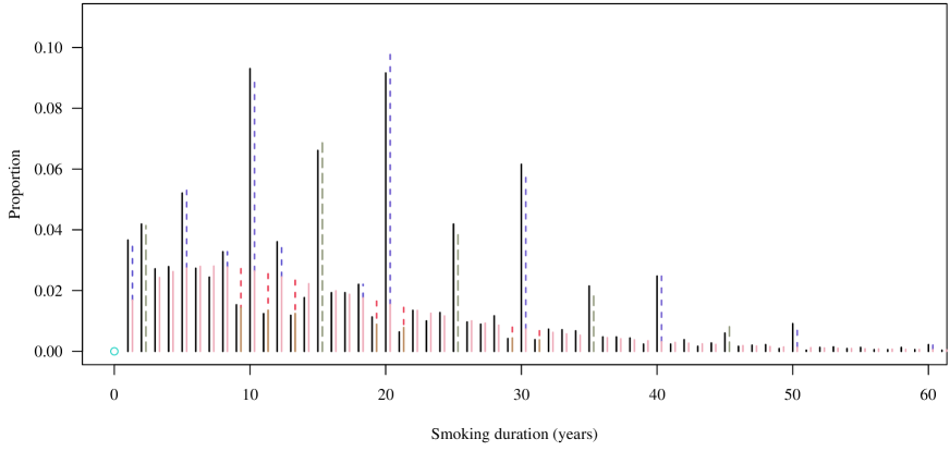
Figure 9: How smokeyears in Fig. 2 and the GAITD regression compare.

Our model showed almost every regression coefficient being very significant (p-value $<0.001$) and $\Xi\approx 41$% of the data was heaped. A rootogram of the fit indicated the response residuals having no systematic lack-of-fit, hence we concluded that the model fitted well to these data.

Next, we added sex and ethnicity to our model. Details of the final model are placed in the Supplementary Materials. Transcribing the coefficients into linear predictors, the model (14) has $\widehat{\mbox{\boldmath$\eta$}}=(\widehat{\eta}_{1},\ldots,\widehat{\eta}_{15})^{T}=\mbox{}$ $\bigg{(}\log\,\widehat{\mu}_{\pi}=2.736+\mathrm{I}(\mathtt{Male})\,0.124-\mathrm{I}(\mathtt{Maori})\,0.262-\mathrm{I}(\mathtt{Polynesian})\,0.238-\mathrm{I}(\mathtt{Other})\,0.217,\ \log\,\widehat{k}_{\pi}=0.631,~{}g(\widehat{\omega}_{p})=-0.976,~{}\log\,\widehat{\mu}_{\alpha}=2.839+\mathrm{I}(\mathtt{Male})\,0.134-\mathrm{I}(\mathtt{Maori})\,0.185-\mathrm{I}(\mathtt{Polynesian})\,0.315-\mathrm{I}(\mathtt{Other})\,0.450,\ \log\,\widehat{k}_{\alpha}=0.806,~{}g(\widehat{\phi}_{p})=-0.622,\ \log\,\widehat{\mu}_{\iota}=3.118+\mathrm{I}(\mathtt{Male})\,0.041-\mathrm{I}(\mathtt{Maori})\,0.137-\mathrm{I}(\mathtt{Polynesian})\,0.189-\mathrm{I}(\mathtt{Other})\,0.395,\ \log\,\widehat{k}_{\iota}=1.476,~{}g(\widehat{\psi}_{p})=-2.110,\ \log\,\widehat{\mu}_{\delta}=\widehat{\eta}_{1},\ \log\,\widehat{k}_{\delta}=\widehat{\eta}_{2},\ g(\widehat{\phi}_{\lceil 1\rceil})=-3.112,~{}g(\widehat{\phi}_{\lceil 8\rceil})=-4.508,~{}g(\widehat{\phi}_{\lceil 12\rceil})=-3.716,~{}g(\widehat{\phi}_{\lceil 18\rceil})=-4.660\bigg{)}^{T}$ where $g$ is the multinomial logit link. In particular, the final model suggests that: (i) Europeans smoke longer than the other three ethnicities—and there appears little difference between the three; (ii) Males smoke longer in general, however there does not seem to be a difference between males and females in the inflated values (spikes).

7 Discussion

This paper extends models commonly known by the abbreviations ZIP, ZAP, ZTP, ZDP, ZINB, ZAB, ZTB, …, into a maximal class of models having four operators with parametric and nonparametric variants operating concurrently. The resultant combo model provides much needed unification. However, even with the limited additional flexibility afforded by having {0} as the only special value, such models have been found easily misused, and guidelines have evolved for fitting them. For example, some authors of software have highlighted common mistakes made by practitioners, e.g., the mgcv 1.8-38 ziP helpfile (Wood, 2017) urges users about checking and cautions about identifiability problems and convergence warnings. These guidelines transfer across to GAITD regression with even greater force, and since GAITD regression is so flexible, it is likely that overfitting will be a common error among novice users.

Another area where practitioners need to exhibit more care is hypothesis testing, e.g., $H_{0}:\phi=0$ for the ZIP. Then the usual regularity conditions do not hold for ordinary likelihood inference at the boundaries and special measures need to be adopted, e.g., Moran (1971), Self and Liang (1987). Many practitioners adopt the Vuong (1989) test, e.g., Greene (2012, pp.574–6,863), however its recommendation is not universal (Wilson, 2015). With GAITD regression the issue is aggravated by having multiple boundaries from the mixing probabilities of GI models.

The choice of the $i_{s}$ warrants comment. As generally-inflated models can easily be overused, selection of the elements of $\mbox{${\cal I}$}_{p}$ and $\mbox{${\cal I}$}_{np}$ should ideally be justified prior to the data being examined, as well as empirical observation of unequivocal excess values. For example, in analyses of 20 multivariate data sets of count data, Warton (2005) concluded that it was rarely necessary to fit 0-inflated models to data sets with high frequencies of 0s when the estimated NB (empirically, the best fitting distribution) mean parameter was low. To quote mgcv: ‘Zero inflated models are often over-used. Having lots of zeroes in the data does not in itself imply zero inflation. Having too many zeroes given the model mean may imply zero inflation.’ For GAITD regression any support value considered inflated should be justified in the context of the entire distribution and parameter values.

A possible consequence of the GT-expansion method is a reduction of the need for developing parametric distributions to handle underdispersion, for example, the Conway–Maxwell–Poisson distribution (e.g., Sellers et al., 2012; Huang, 2017) has seen a revival but is beset by computational difficulties.

We mention two avenues for future work in closing. Firstly, this work very naturally extends to continuous distributions where spikes are augmented by slabs because alteration, inflation and deflation can operate on subintervals. Some preliminary work has already commenced in this area. Secondly, several layers of altered/inflated/deflated values are conceivable, which would entail $\mbox{${\cal A}$}_{1p},\mbox{${\cal A}$}_{2p},\ldots$, and $\mbox{${\cal I}$}_{1p},\mbox{${\cal I}$}_{2p},\ldots$, and $\mbox{${\cal D}$}_{1p},\mbox{${\cal D}$}_{2p},\ldots$ replacing $\mbox{${\cal A}$}_{p}$, $\mbox{${\cal I}$}_{p}$ and $\mbox{${\cal D}$}_{p}$.

Supplementary Materials

The computational and software details placed in the supplementary materials are currently unavailable online. The software implementation is in the VGAM package (version 1.1-6 onwards) on CRAN; please consult the online help for details.

Thomas Yee, Department of Statistics, University of Auckland, New Zealand. E-mail: t.yee@auckland.ac.nz

Chenchen Ma School of Mathematical Sciences and Center for Statistical Science, Peking University, China. E-mail: ChenchenMa@pku.edu.cn

References

- Agresti [2015] A. Agresti. Foundations of Linear and Generalized Linear Models. Wiley, NJ, USA, 2015.
- Berger and Tutz [2021] M. Berger and G. Tutz. Transition models for count data: A: flexible alternative to fixed distribution models. Statist. Meth. & Appl., 30(4):1259–1283, 2021.
- Cameron and Trivedi [2013] A. C. Cameron and P. K. Trivedi. Regression Analysis of Count Data. Cambridge University Press, Cambridge, second edition, 2013.
- Carroll et al. [2006] R. J. Carroll, D. Ruppert, L. A. Stefanski, and C. M. Crainiceanu. Measurement Error in Nonlinear Models: A Modern Perspective. Chapman & Hall/CRC, Boca Raton, FL, USA, second edition, 2006.
- Cox [2004] N. J. Cox. Speaking Stata: Graphing distributions. Stata J., 4(1):66–88, 2004.
- Crawford et al. [2015] F. W. Crawford, R. E. Weiss, and M. A. Suchard. Sex, lies and self-reported counts: Bayesian mixture models for heaping in longitudinal count data via birth-death processes. Ann. Appl. Stat., 9(2):572–596, 2015.
- Fruhwirth-Schnatter et al. [2019] S. Fruhwirth-Schnatter, G. Celeux, and C. P. Robert, editors. Handbook of Mixture Analysis. Chapman and Hall/CRC, Boca Raton, FL, USA, first edition, 2019.
- Greene [2012] W. H. Greene. Econometric Analysis. Prentice Hall, Upper Saddle River, NJ, 7th edition, 2012.
- Haslett et al. [2022] J. Haslett, A. Parnell, J. Hinde, and R. A. Moral. Modelling excess zeros in count data: A new perspective on modelling approaches. International Statistical Review, 90(In press), 2022.
- Heitjan and Rubin [1990] D. F. Heitjan and D. B. Rubin. Inference from coarse data via multiple imputation with application to age heaping. J. Amer. Statist. Assoc., 85(410):304–314, 1990.
- Hirshkowitz et al. [2015] M. Hirshkowitz, K. Whiton, and et al. National Sleep Foundation’s sleep time duration recommendations: methodology and results summary. Sleep Health, 1(1):40–43, 2015.
- Huang [2017] A. Huang. Mean-parametrized Conway–Maxwell–Poisson regression models for dispersed counts. Statist. Model., 17(6):359–380, 2017.
- Karlis and Xekalaki [2005] D. Karlis and E. Xekalaki. Mixed Poisson distributions. International Statistical Review, 73(1):35–58, 2005.
- Kleiber and Zeileis [2008] C. Kleiber and A. Zeileis. Applied Econometrics with R. Springer, New York, USA, 2008. ISBN 978-0-387-77316-2.
- Kullback and Leibler [1951] S. Kullback and R. A. Leibler. On information and sufficiency. Ann. Math. Statist., 22(1):79–86, 1951.
- Lambert [1992] D. Lambert. Zero-inflated Poisson regression, with an application to defects in manufacturing. Techn., 34(1):1–14, 1992.
- MacKenzie et al. [2002] D. I. MacKenzie, J. D. Nichols, G. B. Lachman, S. Droege, J. Royle, and C. A. Langtimm. Estimating site occupancy rates when detection probabilities are less than one. Ecology, 83(8):2248–55, 2002.
- MacMahon et al. [1995] S. MacMahon, R. Norton, R. Jackson, M. Mackie, A. Cheng, S. Vander Hoorn, A. Milne, and A. McCulloch. Fletcher Challenge-University of Auckland Heart & Health Study: Design and baseline findings. New Zealand Med. J., 108:499–502, 1995.
- Moran [1971] P. A. P. Moran. Maximum-likelihood estimation in non-standard conditions. Math. Proc. Cambridge Philos. Soc., 70(3):441–450, 1971.
- Mullahy [1986] J. Mullahy. Specification and testing of some modified count data models. J. Econometrics, 33(2):341–365, 1986.
- Nelder and Wedderburn [1972] J. A. Nelder and R. W. M. Wedderburn. Generalized linear models. J. Roy. Statist. Soc. Ser. A, 135(3):370–384, 1972.
- Otis et al. [1978] D. L. Otis, K. P. Burnham, G. C. White, and D. R. Anderson. Statistical inference from capture data on closed animal populations. Wildlife Monographs, 62:3–135, 1978.
- Ridout et al. [2001] M. Ridout, J. Hinde, and C. G. B. Démetrio. A score test for testing a zero-inflated Poisson regression model against zero-inflated negative binomial alternatives. Biometrics, 57(1):219–223, 2001.
- Self and Liang [1987] S. Self and K.-Y. Liang. Asymptotic properties of maximum likelihood estimators and likelihood ratio tests under nonstandard conditions. J. Am. Stat. Assoc., 82(398):605–610, 1987.
- Sellers and Morris [2017] K. F. Sellers and D. S. Morris. Underdispersion models: Models that are “under the radar”. Comm. Statist.—Theory & Methods, 46(24):12075–12086, 2017.
- Sellers and Raim [2016] K. F. Sellers and A. Raim. A flexible zero-inflated model to address data dispersion. Comput. Statist. Data Anal., 99:68–80, 2016.
- Sellers et al. [2012] K. F. Sellers, S. Borle, and G. Shmueli. The COM-Poisson model for count data: a survey of methods and applications. Appl. Stochastic Models Bus. Ind., 28:104–116, 2012.
- Su et al. [2013] X. Su, J. Fan, R. A. Levine, X. Tan, and A. Tripathi. Multiple-inflation Poisson model with regularization. Statist. Sinica, 23(3):1071–1090, 2013.
- Tang et al. [2015] W. Tang, N. Lu, T. Chen, W. Wang, D. Gunzler, Y. Han, and X. Tu. On performance of parametric and distribution-free models for zero-inflated and over-dispersed count responses. Statist. Med., 34(24):3235–45, 2015.
- Vuong [1989] Quang H. Vuong. Likelihood ratio tests for model selection and nonnested hypotheses. Econometrica, 57(2):307–333, 1989.
- Wang and Heitjan [2008] H. Wang and D. F. Heitjan. Modeling heaping in self-reported cigarette counts. Statistics in Medicine, 27(19):3789–3804, 2008.
- Wang et al. [2012] H. Wang, S. Shiffman, S. D. Griffith, and D. F. Heitjan. Truth and memory: Linking instantaneous and retrospective self-reported cigarette consumption. Ann. Appl. Stat., 6(4):1689–1706, 2012.
- Warton [2005] D. I. Warton. Many zeros does not mean zero inflation: comparing the goodness-of-fit of parametric models to multivariate abundance data. Environmetrics, 16:275–289, 2005.
- Wilson [2015] P. Wilson. The misuse of the Vuong test for non-nested models to test for zero-inflation. Economics Letters, 127:51–53, 2015.
- Wood [2017] Simon N. Wood. Generalized Additive Models: An Introduction with R. Chapman & Hall, New York, USA, 2017.
- Yee and Hastie [2003] T. W. Yee and T. J. Hastie. Reduced-rank vector generalized linear models. Statist. Model., 3(1):15–41, 2003.
- Yee and Wild [1996] T. W. Yee and C. J. Wild. Vector generalized additive models. Journal of the Royal Society, Series B, 58:481–493, 1996.
- Yee [2015] Thomas W. Yee. Vector Generalized Linear and Additive Models with an Implementation in R. Springer, New York, USA, 2015.
- Zuur et al. [2012] A. F. Zuur, A. A. Saveliev, and E. N. Ieno. Zero Inflated Models and Generalized Linear Mixed Models with R. Highland Statistics Ltd., Newburgh, UK, 2012.