BOBA: Byzantine-Robust Federated Learning with Label Skewness

Abstract

In federated learning, most existing techniques for robust aggregation against Byzantine attacks are designed for the IID setting, i.e., the data distributions for clients are independent and identically distributed. In this paper, we address label skewness, a more realistic and challenging non-IID setting, where each client only has access to a few classes of data. In this setting, state-of-the-art techniques suffer from selection bias, leading to significant performance drop for particular classes; they are also more vulnerable to Byzantine attacks due to the increased deviation among gradients of honest clients. To address these limitations, we propose an efficient two-stage method named BOBA. Theoretically, we prove the convergence of BOBA with an error of optimal order. Empirically, we verify the superior unbiasedness and robustness of BOBA across a wide range of models and data sets against various baselines.

1 Introduction

Federated learning (FL) (McMahan et al. 2017) has attracted much research attention in the past decade. It refers to a machine learning system where multiple clients collaboratively train a shared machine learning model under the orchestration of a central server, thus avoiding the leakage of their own private and sensitive data. During training, each client downloads a copy of the shared model from the server, trains the model with local data, and submits a model update to the server for aggregation. In FL, each client’s data is stored locally and invisible to both the server and other clients. FL has wide applications in sales, finance, healthcare (Yang et al. 2019), etc.

FL systems can be vulnerable to attacks and failures (Kairouz et al. 2021; Lyu et al. 2020). In particular, Byzantine attacks can lead to the convergence to an unsatisfactory model or even divergence (Blanchard et al. 2017). A common defending mechanism against Byzantine attacks is to replace the gradients averaging with robust estimation of the center (Chen, Su, and Xu 2017; Yin et al. 2018). These methods have proven Byzantine-robustness when data from different clients are independent and identically distributed (IID). However, the IID assumption is usually violated in real applications. For example, if each client corresponds to a specific user, the data distribution usually varies from user to user. It is unclear how existing robust aggregators are affected by the violation of the IID assumption.

Our work mainly focuses on label skewness, a typical non-IID setting where each client only has access to a few classes of data (Li and Zhan 2021; Shen et al. 2022). In this setting, each client has the same conditional data distribution given labels, but their label distributions can vary a lot. Label skewness degrades the model in two ways. First, it introduces a selection bias of clients. Aggregators tend to select some clients over others across iterations and thus bias the model. Second, it increases the deviation among honest gradients, making existing aggregators more vulnerable to Byzantine attacks. It requires advanced techniques to tackle these challenges in FL with label skewness.

Focusing on label skewness, we find that the gradients of honest clients are distributed near a $(c-1)$-simplex, where $c$ is the number of classes. Based on this, we propose BOBA (Byzantine-rObust and unBiased Aggregator), a two-stage algorithm to estimate this simplex. In the first stage, we robustly estimate the low dimensional affine subspace that the simplex is in and project all gradients to the subspace. In the second stage, we use a few data samples on the server to estimate the $(c-1)$-simplex and further filter out possible Byzantines. With our algorithm, all honest gradients will be preserved with small perturbation, while Byzantine gradients will either be discarded or weakened. We evaluate BOBA theoretically and empirically, proving that it can alleviate selection bias and achieve robustness. We summarize our contributions below:

• We make a systematic analysis of the robustness of FL with label skewness. Specifically, we summarize two novel challenges and propose optimal order robustness to measure the robustness of an aggregator. (Section 3)

• Based on our finding that honest gradients distribute near a $(c-1)$-simplex, we propose BOBA, including an objective addressing both label skewness and robustness, and an efficient optimization algorithm. (Section 4)

• We theoretically derive the gradient estimation error of BOBA and make a convergence analysis. Theoretical results show that BOBA achieves optimal order robustness while baseline aggregators do not. (Section 5)

• We empirically evaluate the unbiasedness and robustness of BOBA across a wide range of models, data sets, and attacks. We show that BOBA outperforms various baseline aggregators, even when they are allowed to leverage additional server data. (Section 6)

2 Related Works

Robustness in FL

There are extensive works of robust aggregators with IID data (Blanchard et al. 2017; Chen, Su, and Xu 2017; Yin et al. 2018; Pillutla, Kakade, and Harchaoui 2022), most of which replace the averaging step on the server with a robust mean estimator. These methods are theoretically proved not to fail arbitrarily in IID settings. However, as shown in our analysis, they suffer from selection bias and increased vulnerability in label skewness settings. A few works have studied robustness with non-IID data by making the clients “more IID”. (Karimireddy, He, and Jaggi 2022) applies bucketing to make the input of the aggregator more homogeneous, while sacrificing some robustness. (Ghosh et al. 2019) divides clients into IID groups and learns global models in each group. A topic related to selection bias is performance fairness, where each client should have similar accuracy. (Hu et al. 2020) introduces a multi-task learning framework to learn a robust and fair global model. However, it is not robust to Byzantine attacks and can only guarantee Pareto optimal. Ditto (Li et al. 2021) learns personalized models to achieve fairness and robustness, but still requires training a robust global model.

Non-IIDness in FL

Besides robustness, non-IIDness also raises optimization challenges in FL. When clients take multiple local steps, non-IIDness makes local updates diverge and thus degrades the model. A common method to handle non-IIDness is to share a limited amount of data as augmentation (Zhao et al. 2018), which can be collected in many real applications. To further protect privacy, some works replace the raw samples with aggregated samples (Yoon et al. 2021), or synthetic samples (Zhang et al. 2021). Compared to them, our work assumes very limited server data.

Label Skewness and Mixture Distribution

Plenty of works focus on label skewness, a particular sub-class of non-IIDness. FedAwS (Yu et al. 2020) studies an extreme case where each client has only access to one class, while FedRS (Li and Zhan 2021) focuses on a general label skewness setting. A related non-IID setting is mixture distribution (Marfoq et al. 2021), where each client’s data distribution is a mixture of several shared distributions with its own mixture weights. BOBA mainly focuses on label skewness and can be easily extended to mixture distribution.

3 FL with Label Skewness

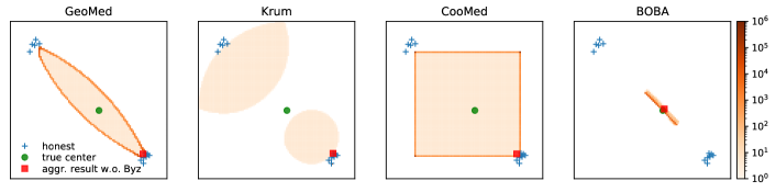
Figure 1: Comparison of aggregation result. Orange set is the range of aggregation results when Byzantines are different. The left three aggregators can have very large aggregation error, while BOBA is much more accurate. See details in Appendix B.2.

Setup

We study the FedSGD (McMahan et al. 2017) system consisting of one central server and $n$ clients. Each client is either honest (in honest set $\mathcal{H}$) or Byzantine (in Byzantine set $\mathcal{B}$). In each communication round, the server broadcasts the parameter ${\boldsymbol{w}}_{G}\in\mathbb{R}^{d}$ to all clients. Each honest client computes the gradient with its own data $\{\boldsymbol{\xi}_{ij}\}_{j=1}^{m}$ sampled from $P_{i}$ and sends back the honest gradient $\boldsymbol{g}_{i}=\nabla_{\boldsymbol{w}_{G}}\mathcal{L}_{i}(\boldsymbol{w}_{G})$, where $\mathcal{L}_{i}(\boldsymbol{w}_{G})=\frac{1}{m}\sum_{j=1}^{m}\mathcal{L}(\boldsymbol{w}_{G};\boldsymbol{\xi}_{ij})$. Each Byzantine client can send arbitrary Byzantine gradient to the server. Finally, the server aggregates all $n$ gradients $\hat{}\boldsymbol{\mu}=\text{Agg}(\{\boldsymbol{g}_{i}\}_{i=1}^{n})$ and updates the parameter $\boldsymbol{w}_{G}\leftarrow\boldsymbol{w}_{G}-\eta\hat{}\boldsymbol{\mu}$, where $\text{Agg}(\cdot)$ is the aggregation function, and $\eta$ is the learning rate. In training phase, the system minimizes the empirical risk, $\frac{1}{|\mathcal{H}|}\sum_{i\in\mathcal{H}}\mathcal{L}_{i}(\boldsymbol{w}_{G})$. Let $|\mathcal{H}|,|\mathcal{B}|$ be the real number of honest and Byzantine clients respectively. As the server does not know the exact number of Byzantines, let $f$ be the declared number of Byzantines, i.e. the max number of Byzantines that the aggregator is robust to.

For each honest client $i\in\mathcal{H}$, let $\mathbb{E}\boldsymbol{g}_{i}$ be its expected gradient, where the expectation is taken on data sampling from $P_{i}$. Let $\boldsymbol{\mu}=\frac{1}{|\mathcal{H}|}\sum_{i\in\mathcal{H}}\boldsymbol{g}_{i}$ denote the gradient of empirical risk and $\mathbb{E}\boldsymbol{\mu}=\frac{1}{|\mathcal{H}|}\sum_{i\in\mathcal{H}}\mathbb{E}\boldsymbol{g}_{i}$ denote its expectation, also the gradient of population risk. Aggregators aim to estimate $\mathbb{E}\boldsymbol{\mu}$ robustly under arbitrary behavior of Byzantine clients.

Distribution of Honest Gradients

This part analyzes the distribution of honest gradients with label skewness. We start with some definitions.

Definition 1 (Inner, outer and total deviations).

For an honest client $i\in\mathcal{H}$, its inner deviation is $\boldsymbol{g}_{i}-\mathbb{E}\boldsymbol{g}_{i}$; its outer deviation is $\mathbb{E}\boldsymbol{g}_{i}-\mathbb{E}\boldsymbol{\mu}$, and its total deviation is $\boldsymbol{g}_{i}-\mathbb{E}\boldsymbol{\mu}$.

Inner deviation measures the randomness of sampling data from clients’ data distribution $P_{i}$, while outer deviation measures the difference from a client’s data distribution $P_{i}$ to the global distribution $P=\frac{1}{|\mathcal{H}|}\sum_{i\in\mathcal{H}}P_{i}$, without randomness.

In the IID setting, the outer deviation is zero, implying that honest gradients $\{\boldsymbol{g}_{i}\}_{i\in\mathcal{H}}$ are distributed around the same center $\mathbb{E}\boldsymbol{\mu}$. When the local batch size $B\to+\infty$, each $\boldsymbol{g}_{i}\stackrel{{\scriptstyle p}}{{\to}}\mathbb{E}\boldsymbol{\mu}$. Such implication does not hold with label skewness, since outer deviations are non-zero. We formally define label skewness and analyze how honest gradients distribute.

Definition 2 ($c$-label skew distribution).

Honest clients’ data distributions $\{P_{i}\}_{i\in\mathcal{H}}$ are $c$-label skew distribution if

$$P_{i}(\boldsymbol{\xi})=\sum_{z=1}^{c}p_{iz}Q_{z}(\boldsymbol{\xi}),\quad\forall i\in\mathcal{H}$$

where $P_{i}(\boldsymbol{\xi})$ is the data distribution of client $i$. The label $z$ can take $c$ finite values. The mixture weight $p_{iz}$ is the label distribution of client $i$ satisfying $\sum_{z=1}^{c}p_{iz}=1$ and the mixture component $Q_{z}(\boldsymbol{\xi})=P_{i}(\boldsymbol{\xi}|z)$ is the conditional distribution given $z$. Different clients share the same $\{Q_{z}(\boldsymbol{\xi})\}_{z=1}^{c}$ but different label distribution $\boldsymbol{p}_{i}=[p_{i1},\cdots,p_{iz}]^{\top}$.

$c$-label skew distribution assumes the heterogeneity among honest clients can be characterized by their divergence in label distribution. With this condition, we can analyze the distribution of honest gradients.

Proposition 1 (Distribution of expected honest gradients).

With $c$-label skew distribution, for any honest client $i\in\mathcal{H}$,

$$\mathbb{E}\boldsymbol{g}_{i} =\sum_{\boldsymbol{\xi}}P_{i}(\boldsymbol{\xi})\nabla_{\boldsymbol{w}}\mathcal{L}(\boldsymbol{w};\boldsymbol{\xi})=\sum_{\boldsymbol{\xi}}\sum_{z=1}^{c}p_{iz}Q_{z}(\boldsymbol{\xi})\mathcal{L}(\boldsymbol{w};\boldsymbol{\xi})$$

$$=\sum_{z=1}^{c}p_{iz}\sum_{\boldsymbol{\xi}}Q_{z}(\boldsymbol{\xi})\mathcal{L}(\boldsymbol{w};\boldsymbol{\xi})=\sum_{z=1}^{c}p_{iz}\mathbb{E}\boldsymbol{\gamma}_{z}$$

where $\mathbb{E}\boldsymbol{\gamma}_{z}=\sum_{\boldsymbol{\xi}}Q_{z}(\boldsymbol{\xi})\mathcal{L}(\boldsymbol{w};\boldsymbol{\xi})$ is the expected gradient computed with data from class $z$.

Proposition 1 shows that each expected honest gradient is a convex combination of $\{\mathbb{E}\boldsymbol{\gamma}_{z}\}_{z=1}^{c}$, whose range forms a $(c-1)$-simplex. We define the honest simplex to be $\{\sum_{z=1}^{c}p_{z}\mathbb{E}\boldsymbol{\gamma}_{z}:\sum_{z=1}^{c}p_{z}=1,p_{z}\geq 0\}$, and the honest subspace to be $\{\sum_{z=1}^{c}p_{z}\mathbb{E}\boldsymbol{\gamma}_{z}:\sum_{z=1}^{c}p_{z}=1\}$.

As honest gradients are perturbations of their expectations, they distribute near the honest simplex, approximately forming a $(c-1)$-dimensional affine subspace. Thus, if we conduct principle component analysis on honest gradients, the variance should concentrate in the first $(c-1)$ principle components. Figure 2 verifies our finding on MNIST. Appendix B.2 gives details of this preliminary experiment.

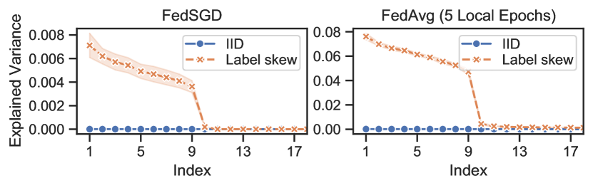
Figure 2: PCA of honest gradients on MNIST ($c=10$)

Notice that the conclusion can be extended to a general mixture distribution (Marfoq et al. 2021) when $z$ is a general latent variable other than the class label, which gives more flexibility. Our paper focuses on label skewness for clarity.

Challenges of Label Skewness

In the IID setting, every honest gradient is an unbiased estimation of $\mathbb{E}\boldsymbol{\mu}$. It is easy to design a robust aggregator since it only needs to find one honest gradient (or a close Byzantine gradient). However, in label skewness settings, each honest gradient can deviate a lot from $\mathbb{E}\boldsymbol{\mu}$. It introduces two challenges to aggregators designed for IID settings: selection bias and increased vulnerability.

Selection bias

Many robust aggregators, including Krum (Blanchard et al. 2017), select a subset of gradients and aggregate. With label skewness, such aggregators select some clients much more often than others. Since each honest gradient is only a biased estimation of $\mathbb{E}\boldsymbol{\mu}$, the aggregation result is also biased, even when there is no Byzantines. In Figure 1 where honest gradients form two clusters, three baseline aggregators all choose the cluster with more clients, resulting in a highly biased aggregation (the red square). Considering each cluster belongs to one class, the model will be trained with one class of data only, resulting in a model predicting every sample as this class.

Increased vulnerability

We observe that the aggregation result can deviate more from the true center $\mathbb{E}\boldsymbol{\mu}$ when the total deviations become larger. Figure 1 shows that the range of aggregation results is huge for IID aggregators, even along the direction where honest gradients do not diverge.

For the two reasons above, although IID aggregators are theoretically robust in IID settings, they have large gradient estimation error even with the absence of Byzantines, and also suffer more with their existence. It is necessary to reconsider the theory of robustness in FL with label skewness.

Optimal Order Robustness

In IID settings, robustness is usually explained as bounded gradient estimation error (Chen, Su, and Xu 2017; Blanchard et al. 2017; Yin et al. 2018). However, such bounds confuse inner and outer deviations, ignore the bias introduced by robust aggregators, and thus can be vacuous (e.g., in Figure 1). Different from them, a good aggregator for label skewness should not bias the aggregation when there are no Byzantines. We define this property as unbiasedness.

Definition 3 (Unbiasedness).

An aggregator $\text{Agg}(\cdot)$ is unbiased if $\text{Agg}(\{\boldsymbol{g}_{i}\}_{i\in\mathcal{H}})\to\mathbb{E}{\boldsymbol{\mu}}$ when $\boldsymbol{g}_{i}\to\mathbb{E}\boldsymbol{g}_{i},\forall i\in\mathcal{H}$; i.e., the aggregator should not introduce additional bias when there are no Byzantines.

However, when there are Byzantine clients, bias is inevitable in label skewness settings. For example, Byzantine clients can mimic the behavior of honest clients (Karimireddy, He, and Jaggi 2022). In this case, any unbiased aggregator should keep them since they are the same as honest ones. With label skewness, such Byzantines can bias the average label distribution by $\|\Delta\bar{}\boldsymbol{p}\|_{1}\leq 2|\mathcal{B}|/n$, introducing an inevitable gradient estimation error of $\mathcal{O}(|\mathcal{B}|/n)$. Based on this fact, we propose optimal order robustness, an adaptive upper bound of gradient estimation error.

Definition 4 (Optimal order robustness).

An aggregator $\text{Agg}(\cdot)$ has optimal order robustness if $\|\text{Agg}(\{\boldsymbol{g}_{i}\}_{i=1}^{n})-\mathbb{E}\boldsymbol{\mu}\|_{2}\to\mathcal{O}(\beta)$ when $\boldsymbol{g}_{i}\to\mathbb{E}\boldsymbol{g}_{i},\forall i\in\mathcal{H}$. $\beta=|\mathcal{B}|/n$ is the fraction of Byzantines.

Unbiasedness can be seen as a special case of optimal order robustness when $\beta=0$. Most robust aggregators designed for IID settings do not have optimal order robustness. Their bias is huge even when $\beta=0$. New aggregators need to be proposed for label skewness settings.

Finally, we extend the necessary condition on the number of Byzantines to achieve robustness from IID to label skewness. IID settings require $n-2f>0$, which means that the honest component should “outweigh” the Byzantine component, i.e., $n-f>f$. However, for $c$-label skew distribution, each component must outweigh the Byzantine component simutaneously. Otherwise, Byzantines can form a cluster to replace a honest component, resulting in unbounded error. Thus, we have the following extended condition.

Condition 1.

Any $n-2f$ expected gradients $\{\mathbb{E}\boldsymbol{g}_{i}\}$ distribute on a $(c-1)$-simplex, but not on any $(c-2)$-simplex.

This condition indicates that any $n-2f$ expectations of honest gradients can uniquely reconstruct the honest simplex. It includes the IID setting when $c=1$. This condition reveals that when $c$ is larger, achieving optimal order robustness is harder since aggregators can tolerate fewer Byzantines. The supremum of $f$ depends on the exact value of label distributions.

4 BOBA Algorithm

Algorithm 1 BOBA(stage 1: line 1-5, stage 2: line 6-10)

0:  $\boldsymbol{G}=[\boldsymbol{g}_{1},\cdots,\boldsymbol{g}_{n}]$, $\boldsymbol{\Gamma}=[\boldsymbol{\gamma}_{1},\cdots,\boldsymbol{\gamma}_{c}]$, $n,f,c,p_{\min}$

0:  Aggregation result $\hat{}\boldsymbol{\mu}$

1:  Initialize subspace $\hat{}\mathcal{P}$: $\boldsymbol{m},\boldsymbol{U},\boldsymbol{\Sigma},\boldsymbol{V}=\text{TrSVD}_{c-1}(\boldsymbol{\Gamma})$

2:  while not converge do

3:     Update $\boldsymbol{r}$: $\boldsymbol{G}_{[n-f]}=\{n-f$ gradients in $\boldsymbol{G}$ with smallest $\|\boldsymbol{g}_{i}-\Pi_{\hat{}\mathcal{P}}(\boldsymbol{g}_{i})\|_{2}\}$ where $\Pi_{\hat{}\mathcal{P}}(\boldsymbol{g}_{i})=\boldsymbol{U}\boldsymbol{U}^{\top}(\boldsymbol{g}_{i}-\boldsymbol{m})+\boldsymbol{m}$

4:     Update $\hat{}\mathcal{P}$: $\boldsymbol{m},\boldsymbol{U},\boldsymbol{\Sigma},\boldsymbol{V}=\text{TrSVD}_{c-1}(\boldsymbol{G}_{[n-f]})$

5:  end while

6:  Encode: $\tilde{\boldsymbol{g}_{i}}=\boldsymbol{U}^{\top}(\boldsymbol{g}_{i}-\boldsymbol{m}),\forall i$; $\tilde{\boldsymbol{\Gamma}}=\boldsymbol{U}^{\top}(\boldsymbol{\Gamma}-\boldsymbol{m}\boldsymbol{1}^{\top})$

7:  Estimate: $\hat{}\boldsymbol{p}_{i}=\left[\begin{matrix}\tilde{\boldsymbol{\Gamma}}\\ \boldsymbol{1}^{\top}\end{matrix}\right]^{-1}\left[\begin{matrix}\tilde{\boldsymbol{g}}_{i}\\ 1\end{matrix}\right],\forall i$

8:  Filter: $\boldsymbol{a}=\mathcal{A}(\{\hat{}\boldsymbol{p}_{i}\}_{i=1}^{n})$

9:  Aggregate: $\tilde{}\boldsymbol{\mu}=\sum_{i=1}^{n}a_{i}\tilde{}\boldsymbol{g}_{i}/\sum_{i=1}^{n}a_{i}$

10:  Decode: $\hat{}\boldsymbol{\mu}=\boldsymbol{U}\tilde{}\boldsymbol{g}_{G}+\boldsymbol{m}$

In this section, we propose BOBA and explain its two stages in detail. In stage 1, we robustly find the honest subspace, and project all gradients to it. In stage 2, we estimate the vertices of the honest simplex, reconstruct the label distribution for each client, and drop clients with abnormal label distribution (i.e., with strongly negative entries). Ideally, all honest gradients will be kept with small perturbation, while all Byzantine gradients will either be weakened (projected to the honest simplex in stage 1) or discarded (in stage 2). Therefore, the impact of Byzantine gradients is limited.

Stage 1: Fitting the Honest Subspace

The goal of stage 1 is to find a $(c-1)$-dimensional affine subspace close to all honest gradients under the influence of Byzantine gradients. When there are no Byzantines, a standard way to find the subspace is TrSVD, i.e., truncated singular value decomposition on centralized gradients,

$$\boldsymbol{m},\boldsymbol{U},\boldsymbol{\Sigma},\boldsymbol{V}=\text{TrSVD}_{c-1}(\boldsymbol{G}),\ \text{s.t.}\ \boldsymbol{U}\boldsymbol{\Sigma}\boldsymbol{V}^{\top}\approx\boldsymbol{G}-\boldsymbol{m}\boldsymbol{1}^{\top}$$

where $\boldsymbol{G}=[\boldsymbol{g}_{1},\cdots,\boldsymbol{g}_{n}]\in\mathbb{R}^{d\times n}$ is the client gradient matrix, $\boldsymbol{m}=\frac{1}{n}\boldsymbol{G}\boldsymbol{1}\in\mathbb{R}^{d}$ is their average, $\boldsymbol{U}\in\mathbb{R}^{d\times(c-1)},\boldsymbol{V}\in\mathbb{R}^{n\times(c-1)}$ are column-orthogonal and $\boldsymbol{\Sigma}\in\mathbb{R}^{(c-1)\times(c-1)}$ is diagonal. TrSVD fits a $(c-1)$-dimensional affine subspace $\mathcal{P}$ minimizing the reconstruction loss

$$\ell(\mathcal{P})=\sum_{i=1}^{n}\left\|\boldsymbol{g}_{i}-\Pi_{\mathcal{P}}(\boldsymbol{g}_{i})\right\|_{2}^{2}$$

where $\Pi_{\mathcal{P}}(\boldsymbol{g}_{i})=\boldsymbol{U}\boldsymbol{U}^{\top}(\boldsymbol{g}_{i}-\boldsymbol{m})+\boldsymbol{m}$ is a projection function that projects vectors to $\mathcal{P}=\{\boldsymbol{U}\boldsymbol{\lambda}+\boldsymbol{m}:\boldsymbol{\lambda}\in\mathbb{R}^{c-1}\}$.

Although vanilla TrSVD is robust to small perturbations (Stewart 1990), it is not Byzantine-robust. When there are Byzantine gradients deviating from the honest subspace, the fitted subspace will be dragged to these Byzantine gradients at the cost of underfitting honest ones. For example in $\mathbb{R}^{2}$, when $n$ honest gradients are uniformly distributed on a segment of $\{(x,y):x\in[-1,1],y=0\}$. TrSVD will fit a subspace of $\{y=0\}$. However, one Byzantine gradient of $(100n,100n)$ can alter the fitted subspace to about $\{y=x\}$.

Objective

Since reconstruction loss is vulnerable, we design trimmed reconstruction loss to robustify TrSVD.

$$\ell_{t}(\mathcal{P})=\min_{\boldsymbol{r}\in\{0,1\}^{n},\atop\sum_{i=1}^{n}r_{i}=n-f}\sum_{i=1}^{n}r_{i}\left\|\boldsymbol{g}_{i}-\Pi_{\mathcal{P}}(\boldsymbol{g}_{i})\right\|_{2}^{2}$$

BOBA stage 1 fits an affine subspace $\hat{}\mathcal{P}$ by minimizing the trimmed reconstruction loss above, which selects the $n-f$ nearest neighbors ($r_{i}=1$) and ignores $f$ gradients furthest from $\hat{}\mathcal{P}$ ($r_{i}=0$). Intuitively, if Byzantines are far from the $\hat{}\mathcal{P}$, they will be ignored so $\hat{}\mathcal{P}$ is not affected; if Byzantine are close to $\hat{}\mathcal{P}$, the $n-f$ nearest neighbors of $\hat{}\mathcal{P}$ still includes at least $n-2f$ honest gradients, which are enough to reconstruct the honest subspace (by Condition 1). We show in Appendix A.5 that stage 1 is theoretically guaranteed to estimate the honest subspace robustly.

Strongest colluding Byzantines may focus on another dimension different from the $c-1$ honest dimensions. But BOBA stage 1 will not identifies the Byzantine dimension as honest. If it makes such mistake, the $n-f$ nearest neighbors will form a $c$-dimensional affine subspace, including one Byzantine dimension and $c-1$ honest dimensions (since there are at least $n-2f$ honest gradients in the $n-f$ nearest neighbors). Conducting TrSVD on them results in non-negligible loss $\propto\delta^{2}$, which can be further optimized. Meanwhile, correctly identifying all honest dimensions results in a loss unrelated to outer deviations, which is much smaller. In our experiments, we also show that BOBA can resist such colluding Byzantines, e.g. Signflip (Xie, Koyejo, and Gupta 2019) and Little (Baruch, Baruch, and Goldberg 2019).

Optimization

To minimize trimmed reconstruction loss, we solve a joint minimization problem

$$\hat{}\mathcal{P},\hat{\boldsymbol{r}}=\operatorname*{argmin}_{\mathcal{P},\boldsymbol{r}\in\{0,1\}^{n},\atop\sum_{i=1}^{n}r_{i}=n-f}\ell_{t}(\mathcal{P},\boldsymbol{r})=\sum_{i=1}^{n}r_{i}\left\|\boldsymbol{g}_{i}-\Pi_{\mathcal{P}}(\boldsymbol{g}_{i})\right\|_{2}^{2}$$

Fixing $\mathcal{P}$, the optimal $\boldsymbol{r}$ selects the $n-f$ nearest neighbors of $\mathcal{P}$; while fixing $\boldsymbol{r}$, the optimal $\mathcal{P}$ can be fitted by conducting TrSVD on the selected $n-f$ gradients. A naive way to minimize trimmed reconstruction loss is exhaustive searching, which iterates every possible value of $\boldsymbol{r}$, conducts TrSVD to fit $\mathcal{P}$, and chooses the $\mathcal{P}$ with the smallest trimmed reconstruction loss. It can guarantee the global minimum but have an exponentially high computational complexity.

Instead, we use alternating optimization, with details in Line 2 - 5 in Algorithm 1. It alternatively updates $\mathcal{P}$ and $\boldsymbol{r}$ until convergence. Although the global minimum may not be guaranteed, alternating optimization can converge to a high-quality local minimum with just a few steps, which is more efficient and practical for large-scale FL.

After minimization, we project every gradient to the fitted subspace $\hat{}\mathcal{P}$. The projection can weaken Byzantine gradients by eliminating its components orthogonal to $\hat{}\mathcal{P}$; meanwhile, it only introduces small bounded perturbation to honest gradients. However, only applying stage 1 does not guarantee robustness: a Byzantine may still have large components along $\hat{}\mathcal{P}$ that bias the aggregation. We design stage 2 to further rule out such Byzantine gradients.

Stage 2: Finding the Honest Simplex

Stage 2 aims to estimate the honest simplex and rule out gradients outside it. Since we have no information on the distribution of clients’ label distributions, it is impossible to estimate the honest simplex with only clients’ gradients. We use a small amount of server data to estimate $c$ vertices of honest simplex, and reconstruct the label distribution of each client. Clients with abnormal label distribution will be discarded.

Proposition 1 shows that each vertex of the honest simplexis the expected gradient computed with one class of data. Thus, we initialize $c$ virtual clients on the server, each with one class of data, and compute server gradients $\{\boldsymbol{\gamma}_{z}\}_{z=1}^{c}$ with the same process of honest clients. To estimate the label distribution of a client $i$, we solve

$$\sum_{z=1}^{c}\hat{p}_{iz}\Pi_{\hat{}\mathcal{P}}(\boldsymbol{\gamma}_{z})=\Pi_{\hat{}\mathcal{P}}(\boldsymbol{g}_{i}),\quad\sum_{z=1}^{c}\hat{p}_{iz}=1$$

Solving this linear system in the gradient space is inefficient. Therefore, we split the projection into two steps: encoding ($\tilde{\boldsymbol{g}}_{i}=\boldsymbol{U}^{\top}(\boldsymbol{g}_{i}-\boldsymbol{m})$) and decoding ($\Pi_{\hat{}\mathcal{P}}(\boldsymbol{g}_{i})=\boldsymbol{U}\tilde{\boldsymbol{g}}_{i}+\boldsymbol{m}$), and solve the linear system in the latent space. The explicit solution is shown in line 6-7 in Algorithm 1.

If our estimation is perfect (e.g. when $\boldsymbol{g}_{i}\to\mathbb{E}\boldsymbol{g}_{i},\boldsymbol{\gamma}_{z}\to\mathbb{E}\boldsymbol{\gamma}_{z}$), $\hat{}\boldsymbol{p}_{i}$ will lie in the probability simplex, i.e. $\{\boldsymbol{p}:\boldsymbol{1}^{\top}\boldsymbol{p}=1,\boldsymbol{p}\geq\boldsymbol{0}\}$ if client $i$ is honest, while it can be arbitrary if client $i$ is Byzantine. So we can discard clients with negative entries in $\hat{}\boldsymbol{p}_{i}$, since they must be Byzantines. However in practice, our estimation has bounded error (Appendix A.6). Thus, if an honest client does not have data from a class, which is very common, it can also have a slightly negative entry. Therefore, we design an acceptance criteria

$$\boldsymbol{a}=\mathcal{A}(\{\hat{}\boldsymbol{p}_{i}\}_{i=1}^{n}),\ \ \text{where }a_{i}=1\text{ if.f. }\min_{z}p_{iz}\geq p_{\min}$$

Here $p_{\min}\leq 0$ is a hyper-parameter deciding the threshold of rejecting Byzantines. In our implementation, we will accept $n-f$ clients with largest $\min_{z=1}^{c}p_{iz}$ if $\sum_{i=1}^{n}a_{i}\leq n-f$, i.e., our acceptance criteria drops too many clients, since there should be at least $n-f$ honest clients. After dropping Byzantines ($a_{i}=0$), we average the remained projected gradients as the aggregation result of BOBA.

Computational complexity

The computational complexity of BOBA is $\mathcal{O}(kcnd)$ if it conducts TrSVD for $k$ times. The complexity of TrSVD is $\mathcal{O}(cnd)$ (Halko, Martinsson, and Tropp 2011), where $c$ is the number of classes, $n$ is the number of clients and $d$ is the dimension of gradient. When $k,c$ are small constants, BOBA has the same complexity as vanilla averaging, which is very efficient. Practically we also observe that $k$ is very small. In three settings with MNIST, CIFAR-10 and AG-News (see Section 6)), $k=3.29,3.20,4.77$ on average.

5 Theoretical Analysis

This section provides theoretical results of the convergence of BOBA and shows that BOBA has optimal order robustness. For space limits, all proofs are deferred to Appendix A. Similar to previous works (Blanchard et al. 2017; Chen, Su, and Xu 2017; Yin et al. 2018), we start with a classical convergence analysis connecting convergence to the gradient estimation error.

Proposition 2.

With $L$-smooth and $\mu$-strongly convex population risk, conducting SGD with gradient $\hat{}\boldsymbol{\mu}$ with estimation error $\|\hat{}\boldsymbol{\mu}-\mathbb{E}\boldsymbol{\mu}\|_{2}\leq\Delta$, and step size $\frac{\mu}{L^{2}}$, after $t$ steps,

$$\|\boldsymbol{w}^{(t)}-\boldsymbol{w}^{*}\|_{2}\leq\left(1-\frac{\mu^{2}}{L^{2}}\right)^{\frac{t}{2}}\|\boldsymbol{w}^{(0)}-\boldsymbol{w}^{*}\|_{2}+\frac{\mu\Delta}{L^{2}-L\sqrt{L^{2}-\mu^{2}}}$$

where $\boldsymbol{w}^{*}$ is the optimal model parameter.

Proposition 2 shows that the parameters exponentially converge to the optimal parameters with an error rate of $\mathcal{O}(\Delta)$. In other words, the gradient estimation error is a good indicator of the error of the model. The following part derives the gradient estimation error of BOBA and test whether it has optimal order robustness. We start with assumptions.

Assumption 1 (Bounded deviations).

1. Honest client inner deviation: with large probability $1-p$ where $p=\mathcal{O}(\frac{1}{\epsilon^{2}})$, $\frac{1}{|\mathcal{H}|}\sum_{i\in\mathcal{H}}\|\boldsymbol{g}_{i}-\mathbb{E}\boldsymbol{g}_{i}\|_{2}^{2}\leq\epsilon^{2}$.

2. Honest client outer deviation: $\|\mathbb{E}\boldsymbol{g}_{i}-\mathbb{E}\boldsymbol{\mu}\|_{2}^{2}\leq\delta^{2},\forall i\in\mathcal{H}$.

3. Server inner deviation: with large probability $1-p_{s}$ where $p_{s}=\mathcal{O}(\frac{1}{\epsilon_{s}^{2}})$, $\frac{1}{c}\sum_{z=1}^{c}\|\boldsymbol{\gamma}_{z}-\mathbb{E}\boldsymbol{\gamma}_{z}\|_{2}^{2}\leq\epsilon_{s}^{2}$.

4. Server outer deviation: $\|\mathbb{E}\boldsymbol{\gamma}_{z}-\mathbb{E}\boldsymbol{\mu}\|_{2}^{2}\leq\delta_{s}^{2},\forall z=1,\cdots,c$.

Assumption 2 (Bounded client singular value).

Conducting centralized SVD on any $n-2f$ expectations of honest gradients, the $(c-1)$-th singular value $\sigma_{c-1}\geq\sigma>0$.

Assumption 3 (Satisfactory optimizer).

There exists a projection function $\mathcal{P}^{\prime}$ fitted by TrSVD on $n-f$ honest gradients with $\ell_{t}(\mathcal{P}^{\prime})\geq\ell_{t}(\hat{}\mathcal{P})$.

Assumption 1 is a deterministic version of bounded inner and outer variation (Wu et al. 2020; Peng, Wu, and Ling 2020), and can be derived from it with Markov inequality. Assumption 2 reformulates Condition 1 with SVD, since the number of non-zero singular values indicates the dimension of a subspace. Assumption 3 says that the optimizer can find a solution that is not too bad (not necessarily the global minimum). This assumption is satisfied in practice since the initialized subspace is fitted by server gradients, which are computed similarly as honest gradients and thus near the honest subspace  $\mathcal{P}^{*}$.

Theorem 3.

With probability at least $1-p-p_{s}$,

$$\|\hat{}\boldsymbol{\mu}-\mathbb{E}\boldsymbol{\mu}\|_{2}\leq\left[1+2\sqrt{\frac{1}{n-2f}+\frac{\delta^{2}}{\sigma^{2}}}\sqrt{|\mathcal{H}|}\right]\epsilon$$

$$+\beta 2(1+c|p_{\min}|)(\sqrt{c}\epsilon_{s}+\delta_{s})$$

where $\beta=|\mathcal{B}|/n$ is the real fraction of Byzantine clients.

When the outer deviation increases $t$ times, both $\delta$ and $\sigma$ increase $t$ times. When all clients are duplicated, $\delta^{2}$ does not change but $\sigma^{2}$ doubled. Thus generally we have $\frac{\delta^{2}}{\sigma^{2}}\propto\frac{1}{n}$. When $\epsilon_{s}=\mathcal{O}(\epsilon),\delta_{s}=\mathcal{O}(\delta)$, $c=\mathcal{O}(1),\frac{1}{n-2f}=\mathcal{O}(\frac{1}{n})$, $|\mathcal{H}|=\mathcal{O}(n)$, and $|p_{\min}|=\mathcal{O}(1)$, we have $\|\hat{}\boldsymbol{\mu}-\mathbb{E}\boldsymbol{\mu}\|_{2}=\mathcal{O}(\epsilon+\beta\delta)$. Let $\epsilon\to 0$, we conclude that BOBA has optimal order robustness, which baseline aggregators do not achieve (see Appendix A.9).

6 Experiments

In this section, we conduct experiments to evaluate the unbiasedness and robustness of BOBA. Specifically, we aim to answer the following research questions.

• RQ1: Is BOBA unbiased when there are no Byzantines?

• RQ2: Is BOBA robust enough to Byzantine attacks?

• RQ3: How do different components contribute to the effectiveness, robustness and efficiency of BOBA?

Table 1: Evaluation of unbiasedness (mean % over 10 runs)

Method	MNIST		CIFAR-10		AG-News
	Acc $\uparrow$	MRD $\downarrow$	Acc $\uparrow$	MRD $\downarrow$	Acc $\uparrow$	MRD $\downarrow$
Average	90.7	-	70.2	-	88.3	-
Server	82.4	17.9	23.4	63.0	81.2	12.8
CooMed	64.7	75.4	19.7	81.4	82.9	10.3
TrMean	76.7	72.3	29.8	79.2	87.0	5.4
Krum	42.4	93.9	32.6	80.8	65.6	89.9
MKrum	89.3	20.1	69.7	9.4	88.0	5.3
GeoMed	90.2	6.1	69.9	4.1	88.3	0.5
B-Krum	70.0	91.5	55.1	80.0	87.6	4.3
B-MKrum	90.3	5.2	69.8	4.2	88.0	3.5
SelfRej	88.9	24.8	69.4	7.3	85.2	20.3
AvgRej	88.6	26.9	69.5	14.7	84.7	22.2
BOBA	90.5	4.5	69.6	2.6	88.3	0.4

Table 2: Evaluation of robustness (mean Acc % over 10 runs)

Method	MNIST				CIFAR-10				AG-News
	Gaussian	Signflip	Little	Worst	Gaussian	Signflip	Little	Worst	Gaussian	Signflip	Little	Worst
Average	9.8	9.8	90.9	9.8	10.0	10.0	65.4	10.0	27.5	25.0	87.6	25.0
CooMed	62.1	42.4	87.3	42.4	20.7	7.7	23.6	7.7	86.0	55.2	81.5	55.2
TrMean	88.6	57.1	83.6	57.1	54.6	13.1	29.7	13.1	88.1	62.4	85.2	62.4
Krum	42.4	42.4	89.7	42.4	36.1	34.7	39.1	34.7	65.8	65.7	80.4	65.7
MKrum	90.8	89.2	90.1	89.2	70.0	54.8	63.7	54.8	88.3	77.0	86.7	77.0
GeoMed	90.2	78.0	89.8	78.0	69.9	46.6	42.0	42.0	88.4	76.2	83.6	76.2
B-Krum	73.6	77.3	89.4	73.6	55.9	56.1	36.5	36.5	88.3	73.3	87.6	73.3
B-MKrum	90.6	88.8	90.1	88.8	70.3	24.3	63.4	24.3	88.3	9.3	85.9	9.3
SelfRej	90.7	68.2	90.2	68.2	70.2	23.3	63.3	23.3	88.3	24.8	86.5	24.8
AvgRej	9.8	90.7	89.6	9.8	10.0	68.3	64.1	10.0	40.8	87.2	84.9	40.8
BOBA	90.7	90.5	90.7	90.5	69.9	68.8	68.2	68.2	88.3	87.9	88.4	87.9

We experiment on a wide range of models and datasets: a 3-layer MLP for MNIST (Lecun et al. 1998), a 5-layer CNN for CIFAR-10 (Krizhevsky and Hinton 2009), and a GRU network for AG-News (Zhang, Zhao, and LeCun 2015). We partition training sets to $|\mathcal{H}|=100,100,160$ honest clients with the method in (McMahan et al. 2017), respectively. For page limits, we give detailed experimental settings and all error bars in Appendix B.1 and B.2.

Byzantines

We consider three types of Byzantines:

• Gaussian (Blanchard et al. 2017), a non-colluding attack uploading large-scale vectors from Gaussian distribution.

• Signflip (Xie, Koyejo, and Gupta 2019), a strong colluding attack uploading $\boldsymbol{g}_{k}=-\gamma\cdot\frac{1}{|\mathcal{H}|}\sum_{i\in\mathcal{H}}\boldsymbol{g}_{i}$, with large $\gamma$ to make Average perform gradient ascent. We set $\gamma=10$ for AG-News and $\gamma=20$ for MNIST and CIFAR-10 (since there are less Byzantines).

• Little (Baruch, Baruch, and Goldberg 2019), a moderate colluding attack uploading vectors within the scope of honest ones to bias the model while avoiding being detected. We set the hyper-parameter according to the original paper, i.e., $z=\phi^{-1}\left((n-\lfloor n/2+1\rfloor)/(n-|\mathcal{B}|)\right)$.

Aggregators

We compare a wide range of baselines:

• Average aggregator (McMahan et al. 2017) simply averages all gradients. It is unbiased but vulnerable to attacks.

• Server aggregator only uses server data to fit a model. We use it to verify that one cannot train a good model with server data only.

• IID aggregators include coordinate median (CooMed) / trimmed mean (TrMean) (Yin et al. 2018), Krum / multi-Krum (MKrum) (Blanchard et al. 2017), and geometric median (GeoMed) (Chen, Su, and Xu 2017).

• Bucketing aggregators (Karimireddy, He, and Jaggi 2022) feed buckets (means) of gradients to IID aggregators. We consider bucketing + Krum (B-Krum) and bucketing + MKrum (B-MKrum) with $s=2$.

• Loss-based rejection aggregators (Fang et al. 2020) detect possible Byzantine clients based on the performance on server data. SelfRej selects $n-f$ clients whose local models $\boldsymbol{w}_{i}=\boldsymbol{w}_{G}-\eta\boldsymbol{g}_{i}$ have smallest loss, while AvgRej selects $n-f$ clients whose gradients can lower the loss of averaged model the most.

All aggregators are set to be robust to $f=16$ Byzantines on MNIST/CIFAR-10 and $f=60$ on AG-News. BOBA uses $p_{\min}=-0.5$. We assume limited server data: 20 per class for MNIST/CIFAR-10 and 30 per class for AG-News, much fewer than the samples on each client.

Unbiasedness and Robustness (RQ1, 2)

Evaluation of unbiasedness

We evaluate the unbiasedness with $|\mathcal{B}|=0$. Besides accuracy, we introduce max-recall-drop (MRD) as a compliment. It computes how the recall scores of each class differ from the model trained with Average (with $|\mathcal{B}|=0$) and picks the largest absolute drop. Smaller MRD indicates a less biased aggregator. As selection bias may dramatically decrease some classes’ recalls while increasing the others, MRD can reflect selection bias better than using accuracy only. Results are shown in Table 1. We observe that BOBA has accuracy very close to Average, and the smallest MRD among all robust aggregators.

Evaluation of robustness

We evaluate the robustness with $|\mathcal{B}|=15,15,54$ on three data sets respectively. Results are shown in Table 2. Notice that Byzantines can choose their attack methods to reduce the model accuracy as much as possible. Therefore, we summarize the worst-case accuracy for a clear comparison in the “worst” column. We observe that BOBA significantly improves the worst-case accuracy by 1.3%, 13.4%, 10.7% on three data sets, respectively.

Discussion of aggregators

Models trained with CooMed and Krum suffer a lot from selection bias, totally fail on some classes. As their natural interpolation with Average, TrMean and MKrum select more clients and thus perform better. MKrum usually has good overall accuracy but still suffers from selection bias and has non-negligible recall drops. GeoMed can be expressed as a positive weighted averaging of all gradients, avoiding dropping useful clients. This property alleviates the selection bias, but also makes GeoMed more vulnerable to Byzantine attacks compared to MKrum. We also observe that bucketing aggregators can alleviate the selection bias of a robust aggregator at the cost of robustness. SelfRej is vulnerable to colluding attacks, while AvgRej is vulnerable to non-colluding Gaussian attacks. Among all aggregators, BOBA is the only method that achieves superior unbiasedness and robustness. It gives uniformly good performance under all settings.

Leveraging server data

Noticing that additional server data may introduce advantages to BOBA, we also study whether server data can enhance baseline aggregators for a fair comparison. We enhance the baselines with $\hat{}\boldsymbol{\mu}=(1-\lambda)\text{Agg}(\{\boldsymbol{g}_{i}\}_{i=1}^{n})+\lambda(\frac{1}{c}\sum_{z=1}^{c}\boldsymbol{\gamma}_{z})$ and test different $\lambda$. Results are given in Appendix B.4, showing that additional server data cannot enhance these aggregators.

Ablation Study (RQ3)

Table 3: Ablation study (mean Acc % over 10 runs)

Method	$|\mathcal{B}|=0$	$|\mathcal{B}|=3$
		Gaussian	Signflip	Little
Average	93.6	83.3	60.6	93.5
Server	84.2	84.2	84.2	84.2
BOBA	93.4	93.6	93.0	93.4
BOBA-ES	93.3	93.6	93.3	93.5
BOBA w.o. stage 1	84.6	85.6	85.5	85.1
BOBA w.o. stage 2	93.4	57.5	39.4	93.4

In this part, we test how each components of BOBA contribute to the aggregation. Since we need to test exhaustive searching, we train a 2-layer MLP on Spambase (Dua and Graff 2017) with $|\mathcal{H}|=12$ honest clients, most of which have only one class of data. We let $f=3,p_{\min}=-0.5$ and assume 30 samples per class. Results are shown in Table 3.

Two Stages

BOBA w.o. stage 1 skips the subspace optimization and uses the subspace initialized with server gradients. It fails to utilize clients’ data, and thus has a worse performance similar to training with server data only. It shows that stage 1 can effectively use clients’ data and thus is necessary. BOBA w.o. stage 2 does not discard any gradients in stage 2. Instead, it averages all projected gradients. It is not robust to large scale Byzantine gradients.

Optimizer

BOBA-ES uses exhaustive searching instead of alternating optimization to fit the honest subspace, which globally minimizes the trimmed reconstruction loss. We observe that BOBA has performance comparable to BOBA-ES. However, it only conducts TrSVD for $<3$ times in average in each rounds, compared to $\binom{n}{f}$ for BOBA-ES.

We can conclude that (1) both stages in BOBA are necessary to guarantee performance and robustness, and (2) alternating optimization significantly improves the efficiency while introducing only marginal performance loss.

7 Conclusion

This paper focuses on Byzantine-robustness in FL with label skewness. We show that existing aggregators suffer from selection bias and increased vulnerability, and propose BOBA to alleviate these problems. We believe robustness has been overlooked in FL, and hope to inspire future works on analyzing robustness with various flexible FL frameworks.

References

- Baruch, Baruch, and Goldberg (2019) Baruch, G.; Baruch, M.; and Goldberg, Y. 2019. A Little Is Enough: Circumventing Defenses For Distributed Learning. In Wallach, H. M.; Larochelle, H.; Beygelzimer, A.; d’Alché-Buc, F.; Fox, E. B.; and Garnett, R., eds., Advances in Neural Information Processing Systems 32: Annual Conference on Neural Information Processing Systems 2019, NeurIPS 2019, December 8-14, 2019, Vancouver, BC, Canada, 8632–8642.
- Blanchard et al. (2017) Blanchard, P.; El Mhamdi, E. M.; Guerraoui, R.; and Stainer, J. 2017. Machine Learning with Adversaries: Byzantine Tolerant Gradient Descent. In Guyon, I.; Luxburg, U. V.; Bengio, S.; Wallach, H.; Fergus, R.; Vishwanathan, S.; and Garnett, R., eds., Advances in Neural Information Processing Systems, volume 30. Curran Associates, Inc.
- Chen, Su, and Xu (2017) Chen, Y.; Su, L.; and Xu, J. 2017. Distributed Statistical Machine Learning in Adversarial Settings: Byzantine Gradient Descent. Proc. ACM Meas. Anal. Comput. Syst., 1(2).
- Dua and Graff (2017) Dua, D.; and Graff, C. 2017. UCI Machine Learning Repository.
- Fang et al. (2020) Fang, M.; Cao, X.; Jia, J.; and Gong, N. Z. 2020. Local Model Poisoning Attacks to Byzantine-Robust Federated Learning. In Capkun, S.; and Roesner, F., eds., 29th USENIX Security Symposium, USENIX Security 2020, August 12-14, 2020, 1605–1622. USENIX Association.
- Ghosh et al. (2019) Ghosh, A.; Hong, J.; Yin, D.; and Ramchandran, K. 2019. Robust Federated Learning in a Heterogeneous Environment. CoRR, abs/1906.06629.
- Halko, Martinsson, and Tropp (2011) Halko, N.; Martinsson, P. G.; and Tropp, J. A. 2011. Finding Structure with Randomness: Probabilistic Algorithms for Constructing Approximate Matrix Decompositions. SIAM Review, 53(2): 217–288.
- Hu et al. (2020) Hu, Z.; Shaloudegi, K.; Zhang, G.; and Yu, Y. 2020. FedMGDA+: Federated Learning meets Multi-objective Optimization. CoRR, abs/2006.11489.
- Kairouz et al. (2021) Kairouz, P.; McMahan, H. B.; Avent, B.; Bellet, A.; Bennis, M.; Bhagoji, A. N.; Bonawitz, K.; Charles, Z.; Cormode, G.; Cummings, R.; D’Oliveira, R. G. L.; Eichner, H.; Rouayheb, S. E.; Evans, D.; Gardner, J.; Garrett, Z.; Gascón, A.; Ghazi, B.; Gibbons, P. B.; Gruteser, M.; Harchaoui, Z.; He, C.; He, L.; Huo, Z.; Hutchinson, B.; Hsu, J.; Jaggi, M.; Javidi, T.; Joshi, G.; Khodak, M.; Konecný, J.; Korolova, A.; Koushanfar, F.; Koyejo, S.; Lepoint, T.; Liu, Y.; Mittal, P.; Mohri, M.; Nock, R.; Özgür, A.; Pagh, R.; Qi, H.; Ramage, D.; Raskar, R.; Raykova, M.; Song, D.; Song, W.; Stich, S. U.; Sun, Z.; Suresh, A. T.; Tramèr, F.; Vepakomma, P.; Wang, J.; Xiong, L.; Xu, Z.; Yang, Q.; Yu, F. X.; Yu, H.; and Zhao, S. 2021. Advances and Open Problems in Federated Learning. Foundations and Trends® in Machine Learning, 14(1–2): 1–210.
- Karimireddy, He, and Jaggi (2022) Karimireddy, S. P.; He, L.; and Jaggi, M. 2022. Byzantine-Robust Learning on Heterogeneous Datasets via Bucketing. In International Conference on Learning Representations.
- Krizhevsky and Hinton (2009) Krizhevsky, A.; and Hinton, G. 2009. Learning multiple layers of features from tiny images. Master’s thesis, Department of Computer Science, University of Toronto.
- Lecun et al. (1998) Lecun, Y.; Bottou, L.; Bengio, Y.; and Haffner, P. 1998. Gradient-based learning applied to document recognition. Proceedings of the IEEE, 86.
- Li et al. (2021) Li, T.; Hu, S.; Beirami, A.; and Smith, V. 2021. Ditto: Fair and Robust Federated Learning Through Personalization. In Meila, M.; and Zhang, T., eds., Proceedings of the 38th International Conference on Machine Learning, ICML 2021, 18-24 July 2021, Virtual Event, volume 139 of Proceedings of Machine Learning Research, 6357–6368. PMLR.
- Li and Zhan (2021) Li, X.; and Zhan, D. 2021. FedRS: Federated Learning with Restricted Softmax for Label Distribution Non-IID Data. In Zhu, F.; Ooi, B. C.; and Miao, C., eds., KDD ’21: The 27th ACM SIGKDD Conference on Knowledge Discovery and Data Mining, Virtual Event, Singapore, August 14-18, 2021, 995–1005. ACM.
- Lyu et al. (2020) Lyu, L.; Yu, H.; Ma, X.; Sun, L.; Zhao, J.; Yang, Q.; and Yu, P. S. 2020. Privacy and Robustness in Federated Learning: Attacks and Defenses. CoRR, abs/2012.06337.
- Marfoq et al. (2021) Marfoq, O.; Neglia, G.; Bellet, A.; Kameni, L.; and Vidal, R. 2021. Federated Multi-Task Learning under a Mixture of Distributions. In Ranzato, M.; Beygelzimer, A.; Dauphin, Y. N.; Liang, P.; and Vaughan, J. W., eds., Advances in Neural Information Processing Systems 34: Annual Conference on Neural Information Processing Systems 2021, NeurIPS 2021, December 6-14, 2021, virtual, 15434–15447.
- McMahan et al. (2017) McMahan, B.; Moore, E.; Ramage, D.; Hampson, S.; and y Arcas, B. A. 2017. Communication-Efficient Learning of Deep Networks from Decentralized Data. In Singh, A.; and Zhu, X. J., eds., Proceedings of the 20th International Conference on Artificial Intelligence and Statistics, AISTATS 2017, 20-22 April 2017, Fort Lauderdale, FL, USA, volume 54 of Proceedings of Machine Learning Research, 1273–1282. PMLR.
- Peng, Wu, and Ling (2020) Peng, J.; Wu, Z.; and Ling, Q. 2020. Byzantine-Robust Variance-Reduced Federated Learning over Distributed Non-i.i.d. Data. CoRR, abs/2009.08161.
- Pillutla, Kakade, and Harchaoui (2022) Pillutla, K.; Kakade, S. M.; and Harchaoui, Z. 2022. Robust Aggregation for Federated Learning. IEEE Transactions on Signal Processing, 70: 1142–1154.
- Shen et al. (2022) Shen, Z.; Cervino, J.; Hassani, H.; and Ribeiro, A. 2022. An Agnostic Approach to Federated Learning with Class Imbalance. In International Conference on Learning Representations.
- Stewart (1990) Stewart, G. W. 1990. Perturbation Theory for the Singular Value Decomposition. Technical report, USA.
- Wu et al. (2020) Wu, Z.; Ling, Q.; Chen, T.; and Giannakis, G. B. 2020. Federated Variance-Reduced Stochastic Gradient Descent With Robustness to Byzantine Attacks. IEEE Transactions on Signal Processing, 68: 4583–4596.
- Xie, Koyejo, and Gupta (2019) Xie, C.; Koyejo, O.; and Gupta, I. 2019. Fall of Empires: Breaking Byzantine-tolerant SGD by Inner Product Manipulation. In Globerson, A.; and Silva, R., eds., Proceedings of the Thirty-Fifth Conference on Uncertainty in Artificial Intelligence, UAI 2019, Tel Aviv, Israel, July 22-25, 2019, volume 115 of Proceedings of Machine Learning Research, 261–270. AUAI Press.
- Yang et al. (2019) Yang, Q.; Liu, Y.; Chen, T.; and Tong, Y. 2019. Federated Machine Learning: Concept and Applications. ACM Trans. Intell. Syst. Technol., 10(2).
- Yin et al. (2018) Yin, D.; Chen, Y.; Kannan, R.; and Bartlett, P. 2018. Byzantine-Robust Distributed Learning: Towards Optimal Statistical Rates. In Dy, J.; and Krause, A., eds., Proceedings of the 35th International Conference on Machine Learning, volume 80 of Proceedings of Machine Learning Research, 5650–5659. PMLR.
- Yoon et al. (2021) Yoon, T.; Shin, S.; Hwang, S. J.; and Yang, E. 2021. FedMix: Approximation of Mixup under Mean Augmented Federated Learning. In 9th International Conference on Learning Representations, ICLR 2021, Virtual Event, Austria, May 3-7, 2021. OpenReview.net.
- Yu et al. (2020) Yu, F. X.; Rawat, A. S.; Menon, A. K.; and Kumar, S. 2020. Federated Learning with Only Positive Labels. In Proceedings of the 37th International Conference on Machine Learning, ICML 2020, 13-18 July 2020, Virtual Event, volume 119 of Proceedings of Machine Learning Research, 10946–10956. PMLR.
- Zhang et al. (2021) Zhang, L.; Shen, B.; Barnawi, A.; Xi, S.; Kumar, N.; and Wu, Y. 2021. FedDPGAN: Federated Differentially Private Generative Adversarial Networks Framework for the Detection of COVID-19 Pneumonia. Inf. Syst. Frontiers, 23(6): 1403–1415.
- Zhang, Zhao, and LeCun (2015) Zhang, X.; Zhao, J. J.; and LeCun, Y. 2015. Character-level Convolutional Networks for Text Classification. In Advances in Neural Information Processing Systems.
- Zhao et al. (2018) Zhao, Y.; Li, M.; Lai, L.; Suda, N.; Civin, D.; and Chandra, V. 2018. Federated Learning with Non-IID Data. CoRR, abs/1806.00582.