Robust 3D Vision for Autonomous Robots

Abstract

This paper presents a fault-tolerant 3D vision system for autonomous robotic operation. In particular, pose estimation of space objects is achieved using 3D vision data in an integrated Kalman filter (KF) and an Iterative Closest Point (ICP) algorithm in a closed-loop configuration. The initial guess for the internal ICP iteration is provided by state estimate propagation of the Kalman filer. The Kalman filter is capable of not only estimating the target’s states, but also its inertial parameters. This allows the motion of the target to be predictable as soon as the filter converges. Consequently, the ICP can maintain pose tracking over a wider range of velocity due to increased precision of ICP initialization. Furthermore, incorporation of the target’s dynamics model in the estimation process allows the estimator continuously provide pose estimation even when the sensor temporally loses its signal namely due to obstruction. The capabilities of the pose estimation methodology is demonstrated by a ground testbed for Automated Rendezvous & Docking (AR&D). In this experiment, Neptec’s Laser Camera System (LCS) is used for real-time scanning of a satellite model attached to a manipulator arm, which is driven by a simulator according to orbital and attitude dynamics. The results showed that robust tracking of the free-floating tumbling satellite can be achieved only if the Kalman filter and ICP are in a closed-loop configuration.

1 Introduction

There are several on-orbit servicing missions on the horizon that will require capabilities for autonomous rendezvous & docking, autonomous rendezvous & capture, proximity operation of space vehicles, constellation satellites, and formation flying [1, 2, 3, 4, 5, 6, 7, 8, 9, 10, 11, 12, 13, 14, 15]. Successful accomplishment of these missions critically relies on a fault-tolerant sensor system to obtain real-time relative pose information (in 6-dof) of two spacecraft during proximity operations. There are different vision systems capable of estimating the pose (position and orientation) of moving objects. However, among them, an active vision system such as the Neptec Laser Camera System (LCS) is preferable because of its robustness in the face of the harsh lighting conditions of space [16, 1]. As verified during the STS-105 space mission, the 3D imaging technology used in the LCS can indeed operate in space environment. The use of laser range data has also been proposed for the motion estimation of free-floating space objects [17, 18]. All vision systems, however, provide discrete and noisy pose data at a relatively low rate, which is typically 1 Hz. It is worth mentioning that another 3D sensor system called TriDAR is an emerging technology that combines the complementary nature of LCS triangulation and Lidar time-of-flight for enhancing the scan range [19, 20].

Vision-based pose estimation algorithms are 3D registration processes, by which the range data set from different views are aligned in a common coordinate system [21, 22]. In general, the 3D registration process consists of two steps: coarse registration and its refinement. The coarse registration process gives a rough estimate of the 3D transformation by using a positioning sensor that is then used as an initial 3D pose in the refinement step. The ICP (Iterative Closest Point) algorithm is the most widely used algorithm as the pose refinement method for geometric alignment of slightly misaligned 3D models [23, 24]. Although the basic ICP algorithm has proven to be very useful in the processing of range data [24], a number of variations on the basic method have been also developed to optimize different phases of the algorithm [24, 25, 11, 26, 27].

Taking advantage of the simple dynamics of a free-floating object, which is not acted upon by any external force or moment, researchers have employed different observers to track and predict the motion of a target satellite [28, 29, 30, 9]. Using the Iterative Recursive Least Squares pose refinement [31], the visual information from camera has been used for relative pose estimation for autonomous rendezvous & docking [32]. In some circumstances, e.g., when there are occlusions, no sensor data is available. Therefore, prediction of the motion of the target based on the latest estimation of its states and dynamic parameters are needed for a continuous pose estimation. This work is focused on the integration of the Kalman filter and the ICP algorithm in a closed-loop configuration for accurate and fault-tolerant pose estimation of a free-falling tumbling satellite [1]. In the conventional pose estimation algorithm, the range data from a rangefinder scanner along with a CAD-generated surface model are used by the ICP algorithm to estimate the target’s pose. The estimation can be made more robust by placing the ICP algorithm and the KF estimator in a closed-loop configuration, wherein the initial guess for the ICP is provided by the estimate prediction [33]. The pose estimation based on the ICP-KF configuration has the following advantages:

1. The KF reduced the measurement noise, thus providing a more precise pose estimation.

2. Faster convergence of the ICP iteration and maintaining tracking over a wider range of object velocity are achieved as a consequence of increased precision of the ICP initial guess provided by the KF.

3. Continuous pose estimation becomes possible even in the presence of temporary sensor failure or obstruction as a consequence of incorporation of the dynamic model of the target in the estimation process.

The KF estimator is designed so that it can estimate not only the target’s states, but also its dynamic parameters. Specifically, the dynamic parameters are the ratios of the moments of inertia of the target, the location of its center of mass, and the orientation of its principal axes. Not only does this allow long-term prediction of the motion of the target, which is needed for motion planning, but also it provides accurate pose feedback for the control system when there are blackout, i.e., no observation data are available [34, 30]. In this work, we use the Euler-Hill equations [35] to derive a discrete-time model that captures the evolution of the relative translational motion of a tumbling target satellite with respect to a chaser satellite which is freely falling in a nearby orbit.

2 ICP Algorithm

This section reviews the basic ICP algorithm originally proposed by Besl and McKay [23]. The ICP algorithm is an iterative procedure which minimizes a distance between point cloud in one dataset and the closest points in the other. Suppose that we are given a 3D point cloud dataset ${\cal U}=\{\bm{u}_{1}\cdots\bm{u}_{m}\}$ that corresponds to a single shape represented by model set ${\cal M}$. It is known that for each point $\bm{u}_{i}\in\mathbb{R}^{3}$ from the 3D points data set ${\cal U}$, there exists at least one point, $\bm{v}_{i}$, on the surface of ${\cal M}$ which is closer to $\bm{u}_{i}$ than other points in ${\cal M}$ [36]. The ICP algorithm assumes that the initial rigid transformation $\{\bm{A}_{0},\bm{r}_{0}\}$ between sets ${\cal U}$ and ${\cal M}$ is known; $\bm{r}_{0}$ and $\bm{A}_{0}$ denote the translation vector and the rotation matrix, respectively. Then, the problem of finding the correspondence between the two sets can be formally expressed by

$$\bm{v}_{i}=\mbox{arg}\min_{\bm{v}_{j}\in{\cal M}}\|\bm{A}_{0}\bm{u}_{i}+\bm{r}_{0}-\bm{v}_{j}\|\qquad\forall i=1,\cdots,m,$$ (1)

and then set ${\cal V}=\{\bm{v}_{1}\cdots\bm{v}_{m}\}$ is formed accordingly. Now, we have two independent sets of 3D points ${\cal V}$ and ${\cal U}$ both of which corresponds to a single shape. The problem is to find a fine alignment $\{\bm{A},\bm{r}\}$ which minimizes the distance between these two sets of points [23]. This can be formally stated as

$$d= \mbox{arg}\min_{\bm{r},\bm{A}}\frac{1}{m}\sum_{i=1}^{m}\|\bm{A}\bm{u}_{i}+\bm{r}-\bm{v}_{i}\|^{2}\qquad\forall\bm{v}_{i}\in{\cal V},\bm{u}_{i}\in{\cal U}$$ (2)

$$\text{s.t.}\quad\bm{A}^{T}\bm{A}=\bm{1}_{3},$$

where $\bm{1}_{3}$ is the $3\times 3$ identity matrix. There are several closed-form solutions to the above least-squares minimization problem [37, 38], of which the quaternion-based algorithm [39] is the preferable choice for $m>3$ over other methods [23]. The rotation matrix can be written as a function of unit quaternion as

$$\bm{A}(\bm{q})=(2q_{o}^{2}-1)\bm{1}_{3}+2q_{o}[\bm{q}_{v}\times]+2\bm{q}_{v}\bm{q}_{v}^{T}.$$ (3)

where $\bm{q}_{v}$ and $q_{o}$ are the vector and scaler parts of the quaternion, i.e., $\bm{q}=[\bm{q}_{v}^{T}\;q_{o}]^{T}$. Consider the cross-covariance matrix of the sets ${\cal V}$ and ${\cal U}$ given by

$$\bm{S}=\mbox{cov}({\cal V},{\cal U})=\frac{1}{m}\sum_{i}\bm{v}_{i}\bm{u}_{i}^{T}-\bar{\bm{v}}\bar{\bm{u}}^{T}$$ (4)

where

$$\bar{\bm{v}}=\frac{1}{m}\sum_{i=1}^{m}\bm{v}_{i}\quad\mbox{and}\quad\bar{\bm{u}}=\frac{1}{m}\sum_{i=1}^{m}\bm{u}_{i}$$ (5)

are the corresponding centroids of the sets. Then, it can be shown that minimization problem (2) is tantamount to find the solution of the following quadratic programming [39]

$$\max_{\|\bm{q}\|=1}\bm{q}^{T}\bm{W}\bm{q}$$ (6)

where the symmetric weighting matrix $\bm{W}$ can be constructed from cross-covariance matrix, $\bm{S}$, as follow

$$\bm{W}=\left[\begin{array}[]{cccc}s_{11}+s_{22}+s_{33}&\times&\times&\times\\ s_{23}-s_{32}&s_{11}-s_{22}-s_{33}&\times&\times\\ s_{31}-s_{13}&s_{21}+s_{12}&-s_{11}+s_{22}-s_{33}&\times\\ s_{12}-s_{21}&s_{31}+s_{13}&s_{23}+s_{32}&-s_{11}-s_{22}+s_{33}\end{array}\right]$$

where $s_{ij}$ denotes the $ij$th entry of matrix $\bm{S}$. The unit quaternion, $\breve{\bm{q}}$, that maximizes the quadratic function of (6) is the eigenvector $\bm{\xi}_{i}$ corresponding to the largest eigenvalue of the matrix $\bm{W}$, i.e., $\breve{\bm{q}}=\bm{\xi}_{i}(\bm{W})$ so that $\lambda_{i}(\bm{W})=\lambda_{\rm max}$. Then, the translation can be obtained from

$$\breve{\bm{r}}=\bar{\bm{v}}-\bm{A}(\breve{\bm{q}})\bar{\bm{u}}$$ (7)

The ICP-based matching algorithm may proceed through the following steps:

1. Given an initial coarse alignment $\{\bm{q}_{0},\bm{r}_{0}\}$, find the closest point pairs ${\cal V}$ from scan 3D points set ${\cal U}$ and model set ${\cal M}$ according to (1).

2. Calculate the fine alignment translation $\{\breve{\bm{q}},\breve{\bm{r}}\}$ minimizing the mean square error the distance between two data sets ${\cal U}$ and ${\cal V}$ according to (6)-(7)

3. Apply the incremental transformation from step ii to step i.

4. Iterate until either the residual error $d$ is less than a threshold, $d_{\rm min}$, or the maximum number of iteration is reached.

It has been shown that the above ICP algorithm is guaranteed to converge to a local minimum [23]. However, a convergence to a global minimum depends on a good initial alignment [40, 41]. In pose estimation of moving objects, “good” initial poses should be provided at the beginning of every ICP iteration. The initial guess for the pose can be taken from the previous estimated pose obtained from the ICP [16]. However, this can make the estimation process fragile when dealing with relatively fast moving target [42]. This is because, if the ICP does not converge for a particular pose, e.g., due to occlusion, in the next estimation step, the initial guess of the pose may be too far from its actual value. If the initial pose happens to be outside the global convergence region of the ICP process, from that point on, the pose tracking is most likely lost for good. The estimation can be made more robust by placing the ICP and a dynamic estimator in a closed-loop configuration, whereby the initial guess for the ICP is provided by the estimate prediction of the moving object. The following sections describe the design of a Kalman filter which will be capable of not only estimating the states but also the parameters of a free-floating object.

3 Motion Dynamics

Fig. 1 illustrates the chaser and the target satellites as rigid bodies moving in nearby orbits. Coordinate frames $\{{\cal A}\}$ and $\{{\cal B}\}$ are attached to the chaser and the target, respectively. The origins of frames $\{{\cal A}\}$ and $\{{\cal B}\}$ are located at center-of-masses (CM)s of the observing and target satellites. The axes of $\{{\cal B}\}$ are chosen to be parallel to the principal axes of the target satellite, while $\{{\cal A}\}$ is orientated so that its $x$-axis is parallel to a line connecting the Earth’s center to the chaser CM and pointing outward, and its $y$-axis lies on the orbital plane; see Fig. 1. The coordinate frame $\{{\cal C}\}$ is fixed to the target at its point of reference (POR) located at distance $\bm{\rho}$ from the origin of $\{{\cal B}\}$. It is the pose of $\{{\cal C}\}$ that is measured by the laser camera. We further assume that the target satellite tumbles with angular velocity $\bm{\omega}$. Also, notice that the coordinate frame $\{{\cal A}\}$ is not inertial; rather, it moves with the chaser satellite. Below, vectors $\bm{\rho}$ and $\bm{\omega}$ are expressed in $\{{\cal B}\}$.

We choose to express the target orientation in the body-attached frames coincident with its principal axes, $\{\cal B\}$, while the translational motion variables are expressed in the body attached frame of the chaser, $\{\cal A\}$. The advantages of such a mixed coordinate selection are twofold: Firstly, the inertia matrix becomes diagonal and will be independent of the target orientation, thus resulting in a simple attitude model. Secondly, choosing to express the relative translational motion dynamics in $\{\cal A\}$ leads to decoupled translational and rotational dynamics that greatly contributes to the simplification of the mathematical model; note that, since $\{\cal B\}$ is a rotating frame, the translational acceleration seen from this frame depends on both the relative angular velocity and relative acceleration. In the following, subscripts $r$ and $t$ denote quantities associated with the rotational and translational dynamics of the system, respectively.

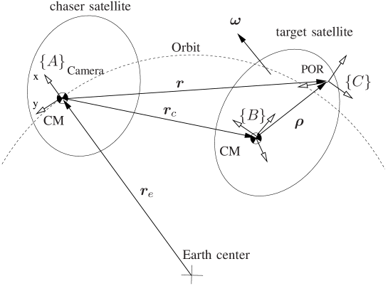
Figure 1: The body-diagram of chaser and target satellites moving in neighboring orbits

3.1 Review of Quaternion Kinematic

In this section, we review some basic definitions and properties of quaternions used in the rest of the paper. Consider quaternions $\bm{q}_{1}$, $\bm{q}_{2}$, $\bm{q}_{3}$ and their corresponding rotation matrices $\bm{A}_{1}$, $\bm{A}_{2}$, and $\bm{A}_{3}$, respectively. Operators $\otimes$ and $\circledast$ are defined as

$$\!\!\!\![\bm{q}\otimes]\triangleq\begin{bmatrix}-[\bm{q}_{v}\times]+q_{o}\bm{1}_{3}&\bm{q}_{v}\\ -\bm{q}_{v}^{T}&q_{o}\end{bmatrix},\quad[\bm{q}\circledast]\triangleq\begin{bmatrix}[\bm{q}_{v}\times]+q_{o}\bm{1}_{3}&\bm{q}_{v}\\ -\bm{q}_{v}^{T}&q_{o}\end{bmatrix}$$

where $[\bm{q}_{v}\times]$ is the cross-product matrix of $\bm{q}_{v}$. Then, $\bm{q}_{3}=\bm{q}_{1}\circledast\bm{q}_{2}\equiv\bm{q}_{2}\otimes\bm{q}_{1}$ corresponds to product $\bm{A}_{3}=\bm{A}_{1}\bm{A}_{2}$. Also, the conjugate quaternion $\bm{q}^{*}$ of $\bm{q}$ is defined such that $\bm{q}^{*}\otimes\bm{q}=\bm{q}\otimes\bm{q}^{*}=[0\;0\;0\;1]^{T}$. Moreover, both $\otimes$ and $\circledast$ operations have associative property, hence $\bm{q}_{1}\otimes\bm{q}_{2}\otimes\bm{q}_{3}$ and $\bm{q}_{1}\circledast\bm{q}_{2}\circledast\bm{q}_{3}$ being unambiguous [43].

The orientation of $\{{\cal A}\}$ with respect to $\{{\cal C}\}$ is represented by the unit quaternion $\bm{q}$, while the orientation of $\{{\cal A}\}$ with respect to $\{{\cal B}\}$ is represented by the unit quaternion $\bm{\mu}$. Moreover, $\bm{\eta}$ is a constant unit quaternion which represent orientation of the principal axes, i.e., orientation of $\{{\cal B}\}$ with respect to $\{{\cal C}\}$. Therefore, the following kinematic relation holds among the aforementioned quaternions

$$\bm{q}=\bm{\eta}\otimes\bm{\mu}.$$ (8)

3.2 State Equations

In the rest of this paper, the underlined form of any vector $\bm{a}\in{\mathbb{R}}^{3}$ denotes the representation of that vector in ${\mathbb{R}}^{4}$, e.g., $\underline{\bm{a}}^{T}\triangleq[\bm{a}^{T}\;0]$. Recall that the orientation of the principal axis of the target satellite with respect to the chaser satellite is represented by a unit quaternion $\bm{\mu}$. The time derivative of $\bm{\mu}$ and the relative angular velocity $\bm{\omega}_{\rm rel}$ are related by

$$\dot{\bm{\mu}}=\frac{1}{2}\underline{\bm{\omega}}_{\rm rel}\otimes\bm{\mu},\qquad\text{where}\qquad\bm{\omega}_{\rm rel}=\bm{\omega}-\bm{\omega}_{n},$$ (9)

and $\bm{\omega}_{n}$ is the angular velocity of the chaser satellite expressed in the frame $\{{\cal B}\}$. Assume that the attitude-control system of the chaser satellite makes it rotate with the angular velocity of the reference orbit. Furthermore, denoting the angular velocity of the reference orbit expressed in $\{{\cal A}\}$ with

$$\bm{n}\equiv\begin{bmatrix}0&0&n\end{bmatrix}^{T},$$ (10)

one can relate $\bm{n}$ and $\bm{\omega}_{n}$ using the quaternion transformation below:

$$\underline{\bm{\omega}}_{n}=\bm{\mu}\otimes\underline{\bm{n}}\otimes\bm{\mu}^{*}.$$ (11)

Substituting (11) into (9) and using the properties of the quaternion products, we arrive at

$$\dot{\bm{\mu}} =\frac{1}{2}\underline{\bm{\omega}}\otimes\bm{\mu}-\frac{1}{2}(\bm{\mu}\otimes\underline{\bm{n}})\otimes(\bm{\mu}^{*}\otimes\bm{\mu})$$

$$=\frac{1}{2}\big{(}\underline{\bm{\omega}}\otimes-\underline{\bm{n}}\circledast\big{)}\bm{\mu}$$ (12)

Define the variation of actual quaternion, $\bm{\mu}$, from its nominal value, $\bar{\bm{\mu}}$, as

$$\delta\bm{\mu}=\bm{\mu}\otimes\bar{\bm{\mu}}^{*}$$ (13)

Then, adopting a technique similar to that used by other authors in  [44, 9], we can linearize the time derivative of the above equation about the estimated states $\bar{\bm{\mu}}$ and $\bar{\bm{\omega}}$ to obtain

$$\frac{d}{dt}\delta\bm{\mu}_{v}\approx-\bar{\bm{\omega}}\times\delta\bm{\mu}_{v}+\frac{1}{2}\delta\bm{\omega}.$$ (14)

Assuming that the spacecraft is acted upon by three independent disturbance torques about its principal axes and denoting the principal moments of inertia as $I_{xx}$, $I_{yy}$, and $I_{zz}$, we can write Euler’s equations as

$$I_{xx}\dot{\omega}_{x} =(I_{yy}-I_{zz})\omega_{y}\omega_{z}+\tau_{x},$$

$$I_{yy}\dot{\omega}_{y} =(I_{zz}-I_{xx})\omega_{z}\omega_{x}+\tau_{y},$$

$$I_{zz}\dot{\omega}_{z} =(I_{xx}-I_{yy})\omega_{x}\omega_{y}+\tau_{z}.$$

Rewriting the above equations in terms of the perturbation $\epsilon_{\tau}=[\tau_{x}/I_{xx}\;\tau_{y}/I_{xx}\;\tau_{z}/I_{xx}]^{T}$, we obtain

$$\dot{\bm{\omega}}=\bm{\psi}(\bm{\omega})+\bm{J}(\bm{p})\bm{\epsilon}_{\tau},$$ (15)

where $\bm{p}^{T}=[p_{x}\thickspace~{}p_{y}\thickspace~{}p_{z}]$, $p_{x}=(I_{yy}-I_{zz})/I_{xx}$, $p_{y}=(I_{zz}-I_{xx})/I_{yy}$, and $p_{z}=(I_{xx}-I_{yy})/I_{zz}$ are the inertia ratios, and

$$\bm{\psi}(\bm{\omega})=\begin{bmatrix}p_{x}\omega_{y}\omega_{z}\\ p_{y}\omega_{x}\omega_{z}\\ p_{z}\omega_{x}\omega_{y}\end{bmatrix},\quad\bm{J}(\bm{p})=\mbox{diag}\Big{\{}1,\;\;\frac{1-p_{y}}{1+p_{x}},\;\;\cfrac{1+p_{z}}{1-p_{x}}\Big{\}}.$$

Linearizing (15) about $\bar{\bm{\omega}}$ and $\bar{\bm{p}}$ yields

$$\delta\dot{\bm{\omega}}=\bm{M}(\bar{\bm{\omega}},\bar{\bm{p}})\delta\bm{\omega}+\bm{N}(\bar{\bm{\omega}})\delta\bm{p}+\bm{J}(\bar{\bm{p}})\bm{\epsilon}_{\tau},$$ (16)

$$\bm{M}(\bm{\omega},\bm{p}) =\frac{\partial\bm{\psi}}{\partial\bm{\omega}}=\begin{bmatrix}0&p_{x}\omega_{z}&p_{x}\omega_{y}\\ p_{y}\omega_{z}&0&p_{y}\omega_{x}\\ p_{z}\omega_{y}&p_{z}\omega_{x}&0\end{bmatrix}$$

$$\bm{N}(\bm{\omega}) =\frac{\partial\bm{\psi}}{\partial\bm{p}}=\begin{bmatrix}\omega_{y}\omega_{z}&0&0\\ 0&\omega_{x}\omega_{z}&0\\ 0&0&\omega_{x}\omega_{y}\end{bmatrix}.$$

The evolution of the relative position of the two satellites can be described by the Euler-Hill model in orbital mechanics. Let the chaser move on a circular orbit with radius $R_{e}$, thus the carrier ray having an angular rate $n$. Further, assume that vector $\bm{r}_{c}$ denotes the relative position of the CM’s of the two satellites expressed in the frame $\{{\cal A}\}$. Then, the translational motion of the target satellite can be expressed as

$$\ddot{\bm{r}}_{c}=-2\bm{n}\times\dot{\bm{r}}_{c}-\bm{n}\times(\bm{n}\times\bm{r}_{c})+\Big{(}-\mu_{e}\frac{\bm{r}_{e}+\bm{r}_{c}}{\|\bm{r}_{e}+\bm{r}_{c}\|^{3}}+n^{2}\bm{r}_{e}\Big{)}+\bm{\epsilon}_{f},$$ (17)

where $\mu_{e}$ is the gravitational parameter of the Earth and $\bm{r}_{e}=[R_{e}\;0\;0]^{T}$ is a constant position vector expressed in frame $\{{\cal A}\}$ that connects the Earth’s center to the chaser CM, and $\bm{\epsilon}_{f}$ denotes the perturbation of translational motion. Note that the constant position vector can be computed from the angular rate of the circular orbit by

$$\bm{r}_{e}=\begin{bmatrix}\sqrt[3]{\cfrac{\mu_{e}}{n^{2}}}&0&0\end{bmatrix}^{T}.$$ (18)

The linearized equations of the translational motion, which are known as the Euler-Hill equations [35] or the Clohessy-Wiltshire equations [45], can be written as

$$\delta\ddot{\bm{r}}_{c}=\bm{K}(n)\delta\bm{r}_{c}-2\bm{n}\times\delta\dot{\bm{r}}_{c}+\bm{\epsilon}_{f},$$ (19)

where $\bm{K}(n)=\mbox{diag}\{3n^{2}\;0\;-n^{2}\}$.

In addition to the inertia of the target satellite, the location of CM, $\bm{\rho}$, and the orientation of the principal axis denoted by unit quaternion, $\bm{\eta}$, are uncertain. Now assume that the state vector to be estimated is:

$$\bm{x}=[\bm{\mu}_{v}^{T}\;\bm{\omega}^{T}\;\bm{p}^{T}\;\bm{r}_{c}^{T}\;\dot{\bm{r}}_{c}^{T}\;\bm{\rho}^{T}\;\bm{\eta}_{v}^{T}]^{T}~{}\in\mathbb{R}^{21}$$ (20)

where $\bm{\eta}_{v}$ is the vector part of unit quaternion $\bm{\eta}$. We assume that the dynamics parameters of the target remain constant, i.e.,

$$\dot{\bm{p}}=\dot{\bm{\rho}}=\dot{\bm{\eta}_{v}}=\bm{0}_{1\times 3}$$ (21)

One can combine the nonlinear equations (12), (15), (17) and (21) in the standard form as $\dot{\bm{x}}=\bm{f}(\bm{x},\bm{\epsilon})$, which can be used for state propagation. However, the KF design also requires the state-transition matrix of the linearized system. Let us define the variation of quaternion $\bm{\eta}$ with respect to its nominal value $\bar{\bm{\eta}}$ according to

$$\delta\bm{\eta}_{=}\bar{\bm{\eta}}^{*}\otimes\bm{\eta}.$$

Then setting the linearized equations (14), (16), and (19) in the standard state-space form yields:

$$\delta\dot{\bm{x}}=\bm{F}\delta{\bm{x}}+\bm{B}\bm{\epsilon}$$ (22)

where vector $\bm{\epsilon}=[\bm{\epsilon}_{\tau}^{T}\;\bm{\epsilon}_{f}^{T}]^{T}$ contains the entire process noise, and

$$\bm{F}=\begin{bmatrix}-[\bar{\bm{\omega}}\times]&\frac{1}{2}\bm{1}_{3}&\bm{0}_{3}&\bm{0}_{3}&\bm{0}_{3}&\bm{0}_{3\times 6}\\ \bm{0}_{3}&\bm{M}(\bar{\bm{\omega}},\bar{\bm{p}})&\bm{N}(\bar{\bm{\omega}})&\bm{0}_{3}&\bm{0}_{3}&\bm{0}_{3\times 6}\\ \bm{0}_{3}&\bm{0}_{3}&\bm{0}_{3}&\bm{0}_{3}&\bm{0}_{3}&\bm{0}_{3\times 6}\\ \bm{0}_{3}&\bm{0}_{3}&\bm{0}_{3}&\bm{0}_{3}&\bm{1}_{3}&\bm{0}_{3\times 6}\\ \bm{0}_{3}&\bm{0}_{3}&\bm{0}_{3}&\bm{K}(n)&-2[\bm{n}\times]&\bm{0}_{3\times 6}\\ \bm{0}_{6\times 3}&\bm{0}_{6\times 3}&\bm{0}_{6\times 3}&\bm{0}_{6\times 3}&\bm{0}_{6\times 3}&\bm{0}_{6}\end{bmatrix},$$

$$\bm{B}=\begin{bmatrix}\bm{0}_{3}&\bm{0}_{3}\\ \bm{J}(\bar{\bm{p}})&\bm{0}_{3}\\ \bm{0}_{6\times 3}&\bm{0}_{6\times 3}\\ \bm{0}_{3}&\bm{1}_{3}\\ \bm{0}_{6\times 3}&\bm{0}_{6\times 3}\end{bmatrix}.$$

The equivalent discrete-time system (22) can be written as

$$\delta\bm{x}_{k+1}=\bm{\Phi}_{k}\delta\bm{x}_{k}+\bm{w}_{k}.$$ (23)

Here the solution to the state transition matrix $\bm{\Phi}_{k}$ and discrete-time process noise $\bm{Q}_{k}=E[\bm{w}_{k}\bm{w}_{k}^{T}]$ can be obtained based on the van Loan method [46] as $\bm{\Phi}_{k}=\bm{D}_{22}^{T}$ and $\bm{Q}_{k}=\bm{\Phi}_{k}\bm{D}_{12}$, where

$$\bm{D}=\begin{bmatrix}\bm{D}_{11}&\bm{D}_{12}\\ \bm{0}&\bm{D}_{22}\end{bmatrix}=\exp\Big{(}\begin{bmatrix}-\bm{F}&\bm{B}\bm{\Sigma}\bm{B}^{T}\\ \bm{0}&\bm{F}^{T}\end{bmatrix}T\Big{)}$$

with $T$ being the sampling time and $\bm{\Sigma}=E[\bm{\epsilon}\bm{\epsilon}^{T}]=\mbox{diag}\{\sigma_{\tau}^{2}\bm{1}_{3},\sigma_{f}^{2}\bm{1}_{3}\}$.

4 Observation Equations

The ICP algorithm gives noisy measurements of the position, $\breve{\bm{r}}$, and orientation, $\breve{\bm{q}}$, of the target. In the followings, the measurement variables will be expressed in terms of the states variables. It is apparent from (1) that

$$\bm{r}=\bm{r}_{c}+\bm{A}(\bm{\mu})\bm{\rho},$$ (24)

Also, recall from (8) that quaternion $\bm{q}$ can be described as a function of $\bm{\eta}$ and $\bm{\mu}$, i.e., $\bm{q}(\bm{\mu},\bm{\eta})=\bm{\eta}\otimes\bm{\mu}$. Consider nominal quaternions $\bar{\bm{\eta}}$ and $\bar{\bm{\mu}}$ which are chosen to be close to the actual quaternions; as will be later discussed in the next section. Then, the variation of the quaternion, $\delta\bm{q}$, with respect to nominal quaternions is defined as

$$\delta\bm{q}=\bar{\bm{\eta}}^{*}\otimes\bm{q}\otimes\bar{\bm{\mu}}^{*}=\delta\bm{\eta}\otimes\delta\bm{\mu}.$$ (25)

Thus, the observation equation can be written as

$$\bm{z}=\bm{h}(\bm{x})+\bm{\nu}$$ (26)

where $\bm{\nu}$ is the measurement noise, which is assumed to be white with the covariance $E[\bm{\nu}\bm{\nu}^{T}]=\bm{R}$, and

$$\bm{z}=\begin{bmatrix}\breve{\bm{r}}\\ \delta\breve{\bm{q}}\end{bmatrix},\qquad\bm{h}(\bm{x})=\begin{bmatrix}\bm{r}_{c}+\bm{A}(\delta\bm{\mu}\otimes\bm{\mu})\bm{\rho}\\ \mbox{vec}(\delta\bm{\eta}\otimes\delta\bm{\eta})\end{bmatrix}.$$ (27)

Note that the observation vector (27) is a nonlinear function of the states[47]. To linearize the observation vector, one also needs to derive the sensitivity of the nonlinear observation vector with respect to the system states. It can readily be seen from (3) that, for a small rotation $\delta\bm{\mu}$, i.e., $\|\delta\bm{\mu}_{v}\|\ll 1$ and $\delta\mu_{0}\approx 1$, the first-order approximation of the rotation matrix can be written as

$$\bm{A}(\delta\bm{\mu})\approx\bm{1}_{3}+2[\delta\bm{\mu}_{v}\times]$$

Hence, (24) can be approximated as

$$\bm{r}\approx\bm{r}_{c}+\bar{\bm{A}}(\bm{\rho}+2\delta\bm{\mu}_{v}\times\bm{\rho}),$$ (28)

where $\bar{\bm{A}}=\bm{A}(\bar{\bm{\mu}})$. Moreover, in view of the definition of the quaternion product and assuming small quaternion variations, we can say that

$$\delta\bm{q}_{v}\approx\delta\bm{\mu}_{v}\times\delta\bm{\eta}_{v}+\delta\bm{\mu}_{v}+\delta\bm{\eta}_{v}.$$ (29)

It is apparent from (28) and (29) that the measurement equations are bilinear functions of the states. Consequently, we can derive the sensitivity matrix $\bm{H}=\frac{\partial\bm{h}}{\partial\bm{x}}$ as

$$\bm{H}=\left[\begin{array}[]{ccccccc}-2\bar{\bm{A}}[\bm{\rho}\times]&\bm{0}_{3}&\bm{0}_{3}&\bm{1}_{3}&\bm{0}_{3}&\bar{\bm{A}}(\bm{1}_{3}+2[\delta\bm{\mu}_{v}\times])&\bm{0}_{3}\\ -[\delta\bm{\eta}_{v}\times]+\bm{1}_{3}&\bm{0}_{3}&\bm{0}_{3}&\bm{0}_{3}&\bm{0}_{3}&\bm{0}_{3}&[\delta\bm{\mu}_{v}\times]+\bm{1}_{3}\end{array}\right]$$

4.1 Filter design

Recall that $\delta\bm{\mu}_{v}$ is a small deviation from the the nominal trajectory $\bar{\bm{\mu}}$. Since the nominal angular velocity $\bar{\bm{\omega}}_{k}$ is assumed constant during each interval, the trajectory of the nominal quaternion can be obtained from

$$\bar{\bm{\mu}}_{k}=e^{\frac{1}{2}T[\hat{\underline{\bm{\omega}}}_{k-1}\otimes}]\hat{\bm{\mu}}_{k-1}.$$

However, since $\bm{\eta}$ is a constant variable, we can say $\bar{\bm{\eta}}_{k}=\hat{\bm{\eta}}_{k-1}$. Let us assume that the state vector is partitioned as $\bm{x}=[\bm{\mu}_{v}^{T}\;\bm{\chi}^{T}\;\bm{\eta}_{v}^{T}]^{T}$. Then, the EKF-based observer for the associated noisy discrete system (23) is given in two steps: ($i$) estimate correction

$$\bm{K}_{k} =\bm{P}_{k}^{-}\bm{H}_{k}^{T}\big{(}\bm{H}_{k}\bm{P}_{k}^{-}\bm{H}_{k}^{T}+\bm{R}_{k}\big{)}^{-1}$$ (30a)

$$\begin{bmatrix}\delta\hat{\bm{\mu}}_{v_{k}}\\ \hat{\bm{\chi}}_{k}\\ \delta\hat{\bm{\eta}}_{v_{k}}\end{bmatrix} =\begin{bmatrix}\delta\hat{\bm{\mu}}_{v_{k}}^{-}\\ \hat{\bm{\chi}}_{k}^{-}\\ \delta\hat{\bm{\eta}}_{v_{k}}^{-}\end{bmatrix}+\bm{K}\big{(}\bm{z}_{k}-\bm{h}(\hat{\bm{x}}_{k}^{-})\big{)}$$ (30b)

$$\bm{P}_{k} =\big{(}\bm{1}_{21}-\bm{K}_{k}\bm{H}_{k}\big{)}\bm{P}_{k}^{-}$$ (30c)

and ($ii$) estimate propagation

$$\hat{\bm{x}}_{k+1}^{-} =\hat{\bm{x}}_{k}+\int_{t_{k}}^{t_{k+1}}\bm{f}(\bm{x}(t),0)\,{\text{d}}t$$ (31a)

$$\bm{P}_{k+1}^{-} =\bm{\Phi}_{k}\bm{P}_{k}\bm{\Phi}_{k}^{T}+\bm{Q}_{k}$$ (31b)

The unit quaternions are computed right after the innovation step (30b) from

$$\hat{\bm{\mu}}_{k} =\begin{bmatrix}\delta\hat{\bm{\mu}}_{v_{k}}\\ \big{(}1-\|\delta\hat{\bm{\mu}}_{v_{k}}\|^{2}\big{)}^{1/2}\end{bmatrix}\otimes e^{\frac{1}{2}T[\hat{\underline{\bm{\omega}}}_{k-1}\otimes]}\hat{\bm{\mu}}_{k-1},$$

$$\hat{\bm{\eta}}_{k} =\begin{bmatrix}\delta\hat{\bm{\eta}}_{v_{k}}\\ \big{(}1-\|\hat{\bm{\eta}}_{v_{k}}\|^{2}\big{)}^{1/2}\end{bmatrix}\odot\hat{\bm{\eta}}_{k-1}.$$

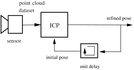
(a) Each ICP iteration uses the last iteration’s pose estimate to seed the next iteration.

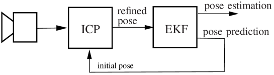
(b) Each ICP iteration uses the KF pose prediction for the time a new dataset is acquired by the sensor.

Figure 2: Pose tracking of moving objects.

4.2 ICP-KF Closed-Loop Configuration

The ICP basically is a search algorithm which tries to find the best possible match between the 3D data of the LCS and a model within the neighborhood of the previous pose. In other words, the LCS sequentially estimates the current pose based on the previous one. That makes the estimation process fragile. This is because if the ICP does not converge for a particular pose, then, in the next estimation step, the initial guess of the pose may be far from the actual one. If the initial pose occurs outside the convergence region of the ICP process, from that point on the pose tracking is lost for good. Fig. 2(a) illustrates the conventional ICP loop where each iteration uses the last iteration’s pose estimate to seed the next iteration either for a fixed number of iterations, fixed time limit, or some convergence criteria are met. The refined pose obtained from the ICP algorithm is then considered as the pose estimation. In this configuration, a new dataset is acquired and the output pose from the last dataset is normally used as the initial pose for the new dataset.

On the other hand, Fig. 2(b) illustrates the ICP and KF in a closed-loop configuration where the refined pose is used as a input to KF while, in turn, the pose prediction of KF is used as the initial pose for the ICP. More specifically, the latter pose estimation process takes the following steps:

1. Refine an initial given pose by applying the ICP iteration on a dataset acquired by the laser sensor.

2. Input the refined pose to the KF in order to filter out the sensor noise and to estimate the object velocities as well as its dynamic parameters.

3. Use the estimation of the states and parameters to propagate the pose at the time when a new dataset is acquired by the sensor.

4. Go to step i and use the pose prediction as the initial pose.

5 Experiment

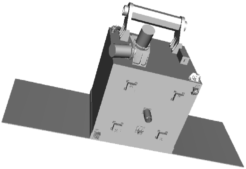
(a) The satellite CAD model.

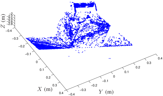
(b) The point-cloud data from scanning of the satellite.

Figure 3: Matching points from the CAD model and the scanned data to estimate the satellite pose.

In this section, experimental results are presented that show comparatively the performance of the pose estimation with and without KF in the loop. The experimental setup includes a satellite mockup attached to a manipulator arm, which is driven by a simulator according to orbital dynamics [1]. The simulator generates the evolution of the relative position and orientation of the two satellites according to (12) and (17). The Neptec laser rangefinder scanner is used to obtain the pose measurements at a rate of 2 Hz. For the spacecraft simulator that drives the manipulator, parameters are selected as

$$\bm{I}_{c}=\begin{bmatrix}4&0&0\\ 0&8&0\\ 0&0&5\end{bmatrix}~{}(\mbox{kgm}^{2})\quad\mbox{and}\quad\bm{\rho}=\begin{bmatrix}-0.15\\ 0\\ 0\end{bmatrix}~{}(\mbox{m}).$$

The solid model of the satellite mockup, Fig. 3(a), and the point-cloud data, generated by the laser rangefinder sensor, Fig. 3(b), are used by the ICP algorithm to estimate the satellite’s pose according to the ICP initialization configurations illustrated in Fig. 2. Three test runs conduced to demonstrate the capability of the estimator are: (i) identification of the spacecraft dynamics parameters, (ii) accuracy and robustness of pose tracking at high velocity.

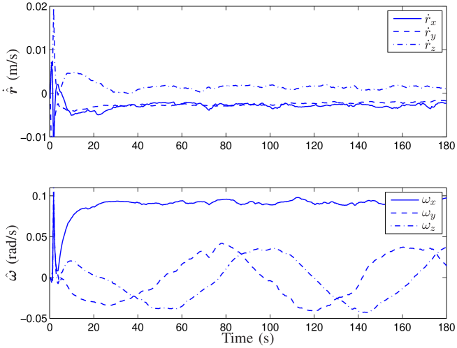
Figure 4: Estimations of the satellite’s linear and angular velocities

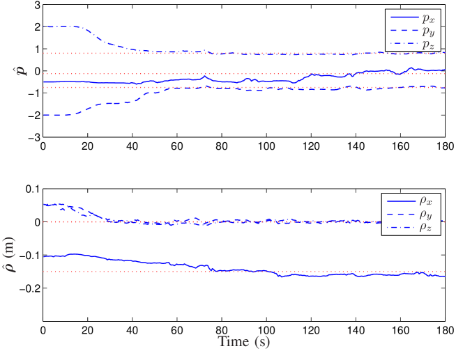
Figure 5: Estimations of the satellite’s dynamics parameters versus their actual values depicted by dotted lines.

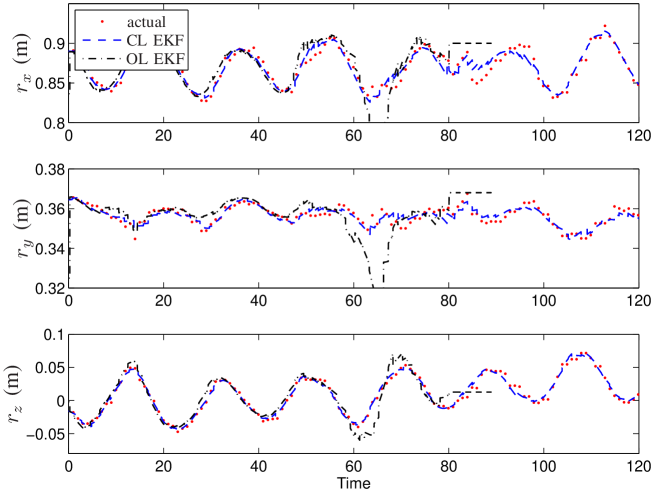
Figure 6: Tracking of the satellite’s position.

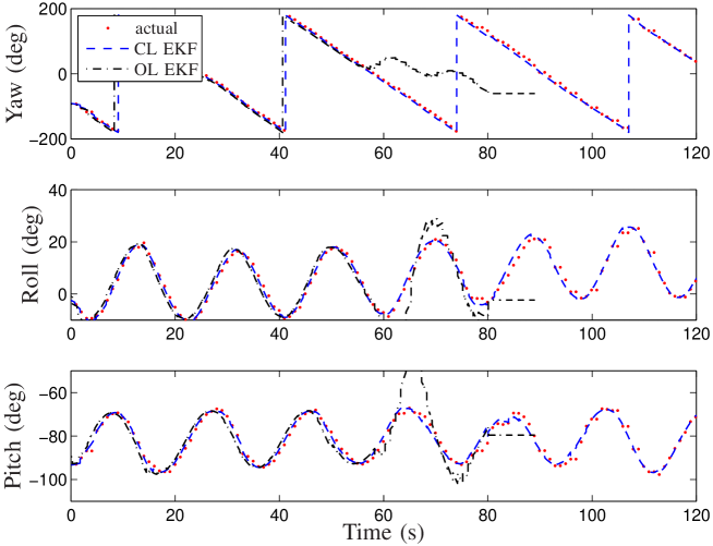
Figure 7: Tracking of the satellite’s attitude.

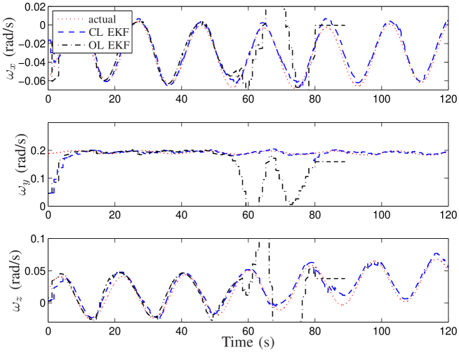
Figure 8: Satellite’s angular velocities.

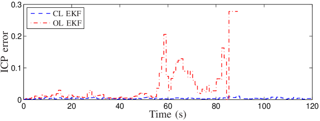
Figure 9: Normalized ICP fit metric.

5.1 Identification of Dynamics Parameters

Figs. 4 and 5 show the trajectories of the estimated velocities and parameters, respectively. The true values of the parameters are depicted by dotted lines in Fig. 5. It is evident from the graphs that the estimated dynamics parameters converged to their true values after about 120 s. The slow convergence rate of the estimator is attributed to the rather small angular velocity of the target satellite. As will be later shown in the following section, the convergence time improves at a higher target velocity.

The robustness of the pose estimation of the tumbling satellite with and without incorporating the KF are comparatively illustrated in Figs 6, 7, and 8. Note that here the quaternion is converted to the the Euler’s angles for representing the orientation. The figures compare the actual trajectories of satellite pose and its angular velocity, obtained by making use of the manipulator kinematic model and measurements of the joint angles and velocities, with those estimated from the vision system. In order to illustrate the importance of the ICP and KF closed-loop configuration in a robust pose estimation, the motion of the target satellites are estimated by two methods: i) Using ICP and EKF in a closed configuration as shown in Fig. 2(b), and ii) cascaded ICP and EKF in an open loop configuration, i.e., the KF does not provide the ICP with the initial guess as shown in Fig. 2(a). The associated trajectories of the former and the later methods are labeled by CL EKF and OL EKF in the figures, respectively. The motion estimation trajectories are compared versus the actual trajectories calculated from the values of the manipulators’ joint angle and velocity measurements by making use of the robot kinematics model. It is evident from the figures that the ICP-based pose estimation is fragile if the initial guess is taken from the last estimated pose. This will cause a growing ICP fit metric over time, as shown in Fig. 9, that eventually leads to a total failure at $t=55$ sec. On the other hand, the pose estimation with the ICP and the KF in the closed-loop configuration exhibits robustness. Trajectories of the estimated angular velocities obtained from the KF versus the actual trajectories are illustrated in Fig. 8. The plot shows that the estimator converges at around $t=8$ s.

6 Conclusion

A robust 3D vision system for autonomous operation of space robots has been presented. A method for pose estimation of free-floating space objects which incorporates a dynamic estimator in the ICP algorithm has been developed. A Kalman filter was used for estimating the relative pose of two free-falling satellites that move in close orbits near each other using position and orientation data provided by a laser vision system. Not only does the filter estimate the system states, but also all the dynamics parameters of the target. Experimental results obtained from scanning a tumbling satellite mockup demonstrated that the pose tracking based on the ICP alone did not converge. On the other hand, the integration scheme of the KF and ICP yielded a robust pose tracking.

References

- [1] F. Aghili, M. Kuryllo, G. Okouneva, and C. English, “Fault-tolerant position/attitude estimation of free-floating space objects using a laser range sensor,” IEEE Sensors Journal, vol. 11, no. 1, pp. 176–185, Jan. 2011.
- [2] F. Aghili, “A prediction and motion-planning scheme for visually guided robotic capturing of free-floating tumbling objects with uncertain dynamics,” IEEE Transactions on Robotics, vol. 28, no. 3, pp. 634–649, June 2012.
- [3] D. Zimpfer and P. Spehar, “STS-71 Shuttle/MIR GNC mission overview,” in Advances in Astronautical Sciences, American Astronautical Society, San Diego, CA, 1996, pp. 441–460.
- [4] F. Aghili, “Automated rendezvous & docking (AR&D) without impact using a reliable 3d vision system,” in AIAA Guidance, Navigation and Control Conference, Toronto, Canada, August 2010.
- [5] T. Laliberte, L. Birglen, and C. Gosselin, “Underactuation in robotic grasping hands,” Japanese Journal of Machine Intelligence and Robotic Control, Special Issue on Underactuated Robots, vol. 43, pp. 77–78, 2002.
- [6] K. Yoshida, “Engineering test satellite VII flight experiment for space robot dynamics and control: Theories on laboratory test beds ten years ago, now in orbit,” The Int. Journal of Robortics Research, vol. 22, no. 5, pp. 321–335, 2003.
- [7] D. R. Wingo, “Orbital recovery’s responsive commercial space tug for life extension missions,” in In Proc. of the AIAA 2nd Responsive Space Conference, Los Angeles, CA, Apr. 2004, pp. 1–9.
- [8] A. Tatsch, N. Fitz-Coy, and S. Gladun, “On-orbit servicing: A brief survey,” in In Proc. of Performance Metrics for Intelligent Systems Conference, Gaithersburg, MD, Aug. 2006.
- [9] F. Aghili and K. Parsa, “Motion and parameter estimation of space objects using laser-vision data,” AIAA Journal of Guidance, Control, and Dynamics, vol. 32, no. 2, pp. 538–550, March 2009.
- [10] B. Liang, C. Li, L. Xue, and W. A. Qiang, “A chinese small intelligent space robotic system for on-orbit servicing,” Beijing, China, Oct. 2006, pp. 4602–4607.
- [11] F. Aghili, M. Kuryllo, G. Okuneva, and D. McTavish, “Robust pose estimation of moving objects using laser camera data for autonomous rendezvous & docking,” in ISPRS Worksshop Laserscanning, Paris, France, September 2009, pp. 253–258.
- [12] C. Kaiser, P. Rank, and R. Krenn, “Simulation of the docking phase for the SMART-OLEV satellite servicing mission,” in International Symposium on Artificial Intelligence, Robotics and Automation in Space (i-SAIRAS), Hollywood, USA, Feb. 2008.
- [13] F. Aghili, “Optimal control for robotic capturing and passivation of a tumbling satellite with unknown dyanmcis,” in AIAA Guidance, Navigation and Control Conference, Honolulu, Hawaii, August 2008.
- [14] F. Aghili and K. Parsa, “Adaptive motion estimation of a tumbling satellite using laser-vision data with unknown noise characteristics,” in 2007 IEEE/RSJ International Conference on Intelligent Robots and Systems, Oct 2007, pp. 839–846.
- [15] F. Aghili, K. Parsa, and E. Martin, “Robotic docking of a free-falling space object with occluded visual condition,” in 9th Int. Symp. on Artificial Intelligence, Robotics & Automation in Space, Los Angeles, CA, Feb. 26 – 29 2008.
- [16] C. Samson, C. English, A. Deslauriers, I. Christie, F. Blais, and F. Ferrie, “Neptec 3D laser camera system: From space mission STS-105 to terrestrial applications,” Canadian Aeronautics and Space Journal, vol. 50, no. 2, pp. 115–123, 2004.
- [17] M. D. Lichter and S. Dubowsky, “State, shape, and parameter estimation of space object from range images,” in IEEE Int. Conf. On Robotics & Automation, New Orleans, Apr. 2004, pp. 2974–2979.
- [18] U. Hillenbrand and R. Lampariello, “Motion and parameter estimation of a free-floating space object from range data for motion prediction,” in The 8th Int. Symposium on Artifcial Intelligence, Robotics and Automation in Space: i-SAIRAS 2005, Munich, Germany, Sep. 5–8 2005.
- [19] C. English, S. Zhu, C. Smith, S. Ruel, and I. Christie, “TriDar: A huybrid sensorfor exploiting the complementary nature of triangulation and lidar technologies,” in International Symposium on Artificial Intelligence, Robotics and Automation in Space (ISAIRAS), Munich, Germany, 5-8 September 2005.
- [20] F. Aghili and C. Y. Su, “Robust relative navigation by integration of icp and adaptive kalman filter using laser scanner and imu,” IEEE/ASME Transactions on Mechatronics, vol. 21, no. 4, pp. 2015–2026, Aug 2016.
- [21] S.-H. Kim, Y.-H. Hwang, H. K. Hong, and M.-H. Choi, Advances in Artificial Intelligence MICAI. Berlin, Heidelberg: Springer, 2004, ch. An Improved ICP Algorithm Based on the Sensor Projection for Automatic 3D Registration, pp. 642–651.
- [22] F. Aghili, “3d simultaneous localization and mapping using IMU and its observability analysis,” Journal of Robotica, December 2010.
- [23] P. J. Besl and N. D. McKay, “A method for registration of 3-D shapes,” IEEE Trans. on Pattern Analysis & Machine Intelligence, vol. 14, no. 2, pp. 239–256, 1992.
- [24] M. Greenspan and M. Yurick, “Approximate K-D tree search for efficient ICP,” in IEEE International Conference on Recent Advances in 3D Digital Imaging and Modeling, Banff, Canada, October 2003, pp. 442–448.
- [25] S. Rusinkiewicz and M. Levoy, “Efficient variants of the ICP algorithm,” in Proc. of 3rd Int. Conf. on 3-D Digital Imaging and Modeling, Quebec City, Canada, 28 May – 1 June 2001, pp. 145–152.
- [26] G. Godin, D. Laurendeau, and R. Bergevin, “A method for the registration of attributed range images,” in Proc. of 3rd Int. Conf. on 3-D Digital Imaging and Modeling, Quebec City, Canada, 28 May – 1 June 2001, pp. 179–186.
- [27] Y. Chen and G. G. Medioni, “Object modeling by registration of multiple range images,” Image and Vision Computing, vol. 10, no. 3, pp. 145–155, 1992.
- [28] F. Aghili, M. Kuryllo, G. Okouneva, and C. English, “Fault-tolerant pose estimation of space objects,” in IEEE/ASME Int. Conf. on Advanced Intelligent Mechatronics (AIM), Montreal, Canada, July 2010, pp. 947–954.
- [29] Y. Masutani, T. Iwatsu, and F. Miyazaki, “Motion estimation of unknown rigid body under no external forces and moments,” in IEEE Int. Conf. on Robotics & Automation, San Diego, May 1994, pp. 1066–1072.
- [30] F. Aghili and K. Parsa, “An adaptive vision system for guidance of a robotic manipulator to capture a tumbling satellite with unknown dynamics,” in IEEE/RSJ Int. Conf. on Intelligent Robots and Systems, Nice, France, September 2008, pp. 3064–3071.
- [31] T. Drummond and R. Cipolla, “Real-time visual tracking of complex structures,” IEEE Trans. on Pattern Analyis and Machine Intelligence, vol. 24, no. 6, pp. 932–946, July 2002.
- [32] J. Kelsey, J. Byrne, M. Cosgrove, S. Seereeram, and R. K. Mehra, “Vision-based relative pose estimation for autonomous rendezvous and docking,” in IEEE Aerospace Conference, Big Sky, MT, 5-8 September 2006, pp. 1–20.
- [33] F. Aghili and A. Salerno, Multisensor Attitude Estimation and Applications, 1st ed. CRC Press, 2016, ch. Adaptive Data Fusion of Multiple Sensors for Vehicle Pose Estimation.
- [34] F. Aghili, M. Kuryllo, G. Okouneva, and C. English, “Robust vision-based pose estimation of moving objects for automated rendezvous & docking,” in IEEE Int. Conf. on Mechatronics and Automation (ICMA), Xian, China, August 2010, pp. 305–311.
- [35] M. H. Kaplan, Modern Spacecraft Dynamics and Control. New York: Wiley, 1976.
- [36] D. A. Simon, M. Herbert, and T. Kanade, “Real-time 3-d estimation using a high-speed range sensor,” in IEEE Int. Conference on Robotics & Automation, San Diego, CA, May 1994, pp. 2235–2241.
- [37] O. D. Faugeras and M. Herbert, “The representation, recognition, and locating of 3-d objects,” The International Journal of Robotics Research, vol. 5, no. 3, pp. 27–52, 1986.
- [38] D. Eggert, A. Lorusso, and R. B. Fisher, “Estimating 3-D rigid body transformation: a comparison of four major algorithms,” Machine Vision & Apllications, vol. 9, no. 5, March 1997.
- [39] B. K. P. Horn, “Closed-form solution of absolute orientation using unit quaternions,” J. Opt. Soc. Amer., vol. 4, no. 4, pp. 629–642, Apr. 1987.
- [40] F. Aghili and A. Salerno, “Driftless 3D attitude determination and positioning of mobile robots by integration of IMU with two RTK GPSs,” IEEE/ASME Trans. on Mechatronics, vol. 18, no. 1, pp. 21–31, Feb. 2013.
- [41] B. B. Amor, M. Ardabilian, and L. Chen, “New experiments on icp-based 3d face recognition and authentication,” in IEEE Int. Conference on Pattern Recognition, Hong Kong, August 2006, pp. 1195–1199.
- [42] F. Aghili and A. Salerno, “3-D localization of mobile robots and its observability analysis using a pair of RTK GPSs and an IMU,” in IEEE/ASME Int. Conf. on Advanced Intelligent Mechatronics (AIM), Montreal, Canada, July 2010, pp. 303–310.
- [43] ——, “Attitude determination and localization of mobile robots using two RTK GPSs and IMU,” in IEEE/RSJ International Conference on Intelligent Robots & Systems, St. Louis, USA, October 2009, pp. 2045–2052.
- [44] E. J. Lefferts, F. L. Markley, and M. D. Shuster, “Kalman filtering for spacecraft attitude estimation,” vol. 5, no. 5, pp. 417–429, Sep.–Oct. 1982.
- [45] W. H. Clohessy and R. S. Wiltshire, “Terminal guidance system for satellite rendezvous,” Journal of Aerosapce Science, vol. 27, no. 9, pp. 653–658, 1960.
- [46] C. F. van Loan, “Computing integrals involving the matrix exponential,” IEEE Trans. on Automatic Control, vol. 23, no. 3, pp. 396–404, Jun. 1978.
- [47] F. Aghili, “Integrating IMU and landmark sensors for 3D SLAM and the observability analysis,” in Proc. of IEEE/RSJ International Conference on Intelligent Robots and Systems (IROS), Taipei, Taiwan, Oct. 2010, pp. 2025–2032.