Simulation Framework for studying MPGD-based DHCAL
Abstract
Digital Hadronic Calorimeters (DHCAL) were suggested for future Colliders as part of the particle-flow concept. Though studied mostly with Resistive Plate Chambers (RPC), studies focusing on Micro-Pattern Gaseous Detector (MPGD)-based sampling elements have shown the potential advantages using such techniques. In 2018, six Micromegas (MM) and two Resistive-Plate WELL (RPWELL) sampling elements were assembled into a small MPGD-based SDHCAL prototype with steel absorber plates. The prototype was tested in low-energy (2-6 GeV) pions at the CERN/PS beam line. We used the collected data to validate a GEANT4-based simulation framework of an MPGD-based DHCAL prototype. The expected pion energy resolution of a full-scale RPWELL-based DHCAL prototype was studied in using this framework for different sampling elements MIP detection efficiency and pad-multiplicity distributions.
1 Introduction
Particle-flow [1] is a leading approach towards reaching the challenging jet energy resolution () [1] required in future lepton collider experiments [2, 3, 4, 5]. Particle-flow calorimeters require high transverse and longitudinal granularity, and therefore many readout channels, to better associate energy deposits with the individual constituent particles of a jet. Digital and Semi-Digital Hadronic Calorimeters ((S)DHCAL) [6] with an 1-2 bit ADC readout are appealing, offering a cost-effective solution for reading out large number of channels.
A typical (S)DHCAL is a sampling calorimeter consisting of alternating layers of absorbers and sampling elements. Hadrons are more likely to interact with the absorber, forming hadronic showers. The shower fragments induce signals on the pad-readout of the sampling elements. The absorber thickness, typically 2 cm for steel, and the pads’ size, typically 1 cm2, defines the longitudinal and transverse granularity, respectively.
Using a DHCAL, the energy measurement of a single particle is reconstructed from the number, and possibly the pattern, of all fired pads (hits). Thus, a high performing sampling element is characterized by high minimum-ionizing particle (MIP) detection efficiency and low average pad-multiplicity. The latter is defined by the number of pads firing per impinging particle. Another important characteristic is the sampling element uniformity.
Sampling elements of different technologies have been studied: 1 m2 glass-RPC [10], 1 m2 Micromegas (MM) [11], 3030 cm2 double Gaseous Electron Multipliers (GEM) [13], 50100 cm2 RWELL [14] , and 3030 cm2 the Resistive-Plate WELL (RPWELL) [15]. Their measured performance is summarized in Table 1. As can be seen, the average pad-multiplicity of the RPC prototype is larger than that of the others. Another advantage of the MPGD technologies is their operation in environment-friendly gas mixtures.
| Average Pad-Multiplicity | efficiency | |
|---|---|---|
| Glass RPC | 1.6 | 98% |
| MM | 1.1 | 98% |
| Resistive MM | 1.1 | 95% |
| Double GEM | 1.2 | 98% |
| RWELL | Not Reported | 96% |
| RPWELL | 1.2 | 98% |
The development of production techniques for scaling up the RPWELL-based sampling elements to 1 m2 is ongoing [15, 17, 18, 19, 20]. In November 2018, we operated a small DHCAL prototype consisting of six MM-based sampling elements and two RPWELL-based sampling elements at the CERN/PS test-beam facility [21, 22]. The WELL electrode used for the RPWELL elements had thickness variations of the order of 20% resulting in gain variations of 250% [23] . Furthermore, the assembly technique had a few weaknesses and potentially resulted in electrical instabilities due to glue penetration in to the RPWELL holes. Nevertheless, they were used, operated at low efficiency, due to time constraints imposed by the LHC long shutdown (2019-2021).
In this work, we validated a GEANT4-based simulation framework of MPGD-based DHCAL with the data collected at the test beam. Using the validated framework, we simulated and evaluated the expected performance of a full-scale (50 layers) RPWELL-based DHCAL. The test beam setup, methods to measure single sampling element performance, simulation framework, and validation methodology are described in Section 2, followed by the validation results in section 3. In Section 4, the expected performance of a full-scale (50 layers) RPWELL-based DHCAL is detailed. The study is summarized in Section 5.
2 Methodology
2.1 Experimental Setup
In November 2018, the small MPGD-based DHCAL prototype was investigated in CERN/PS with low energy (2-6 GeV/c) pion beam. The prototype comprised eight alternating layers of absorber plates and sampling elements [20]. The former consists of 2 cm thick steel plates, a total of 16 cm, corresponding to 0.8 pion interaction length () and 8.9 radiation length (), yielding a 45% (99.9%) chance of a pion (electron) shower to start within the calorimeter. The sampling elements consist of three 1616 cm2 bulk MM (two non-resistive and one resistive), three 4848 cm2 resistive MM, and two 5050 cm2 RPWELL. A schematic description of the experimental setup is given in Figure 1. All eight sampling elements were equipped with semi-digital readout electronics based on the MICROROC/ASU [24]. The small bulk MMs comprised a squared geometry pad-matrix, while the large MM and the RPWELL were equipped with a circular geometry pad-matrix (48 cm diameter) to reduce the number of channels. All the readout pads were 11 cm2. The chambers were operated in a digital mode, where only the lowest threshold of the MICROROC (set to 0.8 fC) was used. All the chambers were read out with a single DAQ system. A trigger region of 1×1 cm2 at the center of the DHCAL X-Y plane was defined by three scintillators, minimizing the transverse energy leakage of the measured showers. The total beam area was 4080 cm2. The RPWELL design is detailed in [20]. As mentioned earlier, these sampling elements were operated below the efficiency plateau. The voltage applied on the WELL electrode () and the drift cathode () were set to 1525 V and 1675 V, respectively. The MM sampling elements were operated at =480 V and =550 V.

2.2 Measuring Sampling Elements Performance
The performance of each sampling element in terms of MIP detection efficiency and pad-multiplicity distribution was measured using MIP tracks – pions that did not initiate a shower. These tracks were reconstructed from hits recorded by the other seven layers (reference layers) using Hough transform [25]. To ensure high quality MIP tracks, we selected only those parallel to the beam axis with exactly one hit in each of the reference layers. These hits had to be close to the reconstructed track (less than a single pad away). A group of hits in the layer X with sharing borders pads formed a cluster, and its position was defined by the averaged position of the cluster hits. An event is considered efficient if cluster position was within 1 cm from the MIP track intersection point with layer X. The pad-multiplicity per event was defined by the number of hits in the cluster of an efficient event.
In addition to the measured MIP detection efficiency and the pad-multiplicity, we also distinguish the hit detection efficiency (HDE) and the true pad-multiplicity. These distinguished properties play an essential role in the emulation of a sampling element response. Let us consider an energy deposit of a traversing particle in a sampling element. Such energy deposit is typically in the form of a cluster of electrons. The electrons are multiplied and induce signals on the readout pads. The HDE is defined as the probability of a pad to detect a hit, and the true pad-multiplicity is defined by the number of pads with induced signals (including signals below a set threshold). Therefore, while the HDE is a characteristic of a single pad, the MIP detection efficiency is less local as it relies on more than a single firing pad contributes to this efficiency. In addition, the measured pad-multiplicity incorporates the effect of the HDE on the true pad-multiplicity. From these relations, we estimated HDE and the true pad-multiplicity from the measurements of the MIP detection efficiency and the pad-multiplicity distribution. Appendix A presents the calculation of such estimation. The true pad-multiplicity and the HDE are used in the simulation framework to emulate the response of the sampling elements.
2.3 Simulation Framework
We developed a GEANT4-based (version 10.06.p01 [26]) simulation to investigate the expected performance of an RPWELL-based DHCAL and optimize the sampling element design. It was validated by comparing the results of a simulated MPGD-based DHCAL to the data measured in the beam.
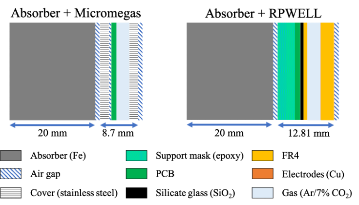
A GEANT4-based software simulates the interactions of the impinging particles with the calorimeter material. The schematic of the DHCAL modules modeling is given in Figure 2. It consists of alternating absorber (iron) layers, air gaps, and sampling elements. The RPWELL layers are defined by a support mask (epoxy), printable circuit board (PCB), gas (Ar/7% CO2), FR4, electrodes (Cu), and silicate glass (SiO2), while the MM layers consist of PCB, gas, and steel covers.
We tested three GEANT4 physics lists to get the best agreement between the data and the simulation: QGSP_BERT, QGSP_BERT_EMZ, and FTFP_BERT_EMZ. Their names indicate the physical models included in them. The EMZ model indicates a high precision modeling of electromagnetic interactions. Further details on the physics lists can be found in [27, 28].
The detector response, the translation of energy deposits into electronic signals, depends on its performance, particularly its detection efficiency and pad-multiplicity. It yields a set of digital electronic signals associated with specific pads for each particle. This response is not modeled by the GEANT4 simulation but with a dedicated digitization script that uses the output of the GEANT4 as an input. For each particle, the latter contains, among others, the particle ID and the information regarding its energy deposits (magnitude, position, and time).
The digitization is implemented using the following steps. First, the energy deposits outside the acceptance region are ignored, and those that are inside that region are assigned a pad position based on geometrical considerations. In the second step, hits in neighboring pads are added, reflecting the true pad-multiplicity distribution. Finally, HDE is applied to all the hits, which means that inefficient hits are deleted.
2.4 Validation Methodology
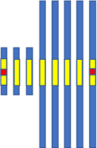
The simulation framework was validated by comparing the simulated response to a measured one. Following the tested DHCAL prototype (subsection 2.1), we modeled an eight-layers DHCAL prototype (Figure 2) and simulated its response to low-energy pions (2, 3, 4, 5, and 6 GeV). For each beam energy, we simulated 50k single pion events. The validation of the simulation consists of two steps. In the first, which can be thought of as a closure test, we verified that the performance of each simulated sampling element (MIP detection efficiency and average pad-multiplicity) is consistent with the experimentally measured values. The second step compares the calorimeter’s response – i.e., the distribution of the total number of hits per event for given pion energy. Two types of event selections were applied to minimize uncertainties originating from the limited acceptance of our DHCAL prototype:
-
1.
MIP-like selection: events with a single hit in the first and last sampling element and not more than 3 hits per sampling element (Figure 3-a).
-
2.
Generic selection: events with exactly one hit in each of the three small sampling ele-ments and no hits outside the expected shower-cone region (marked in yellow in Figure 3-b).

3 Results
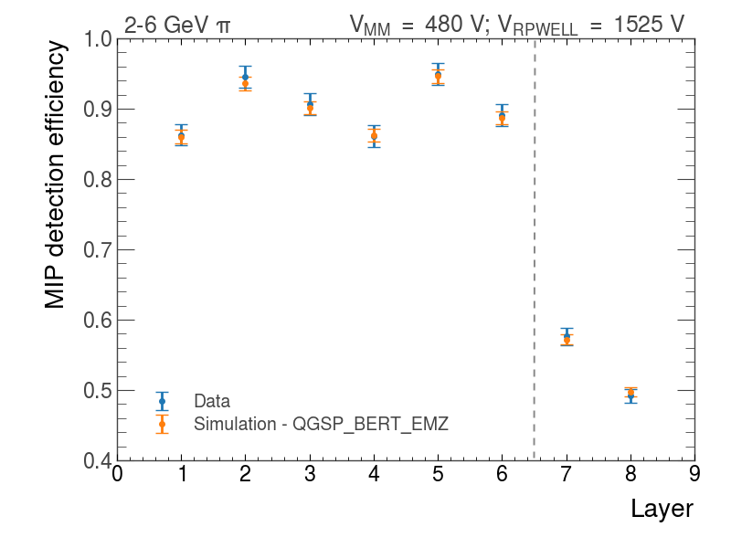
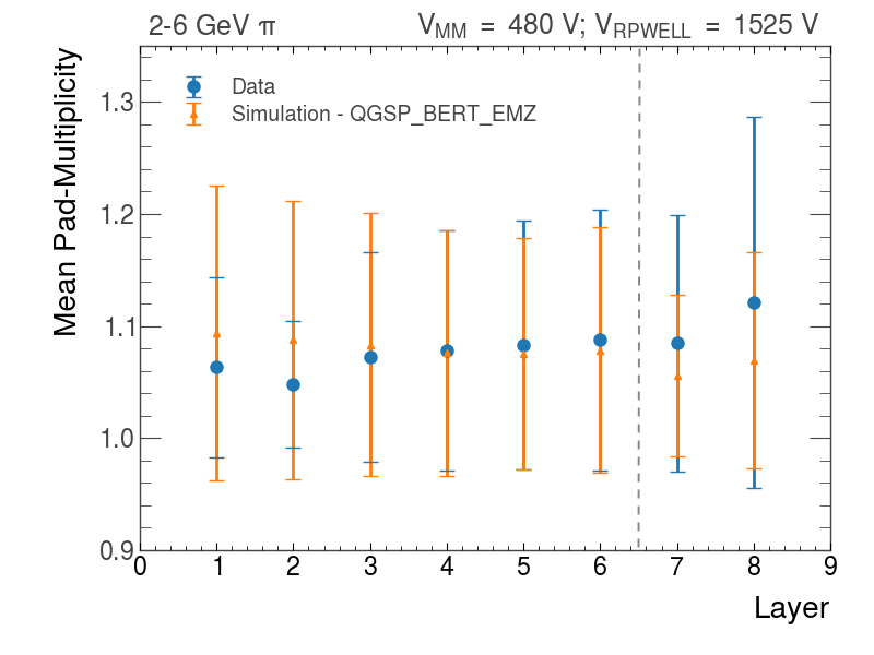
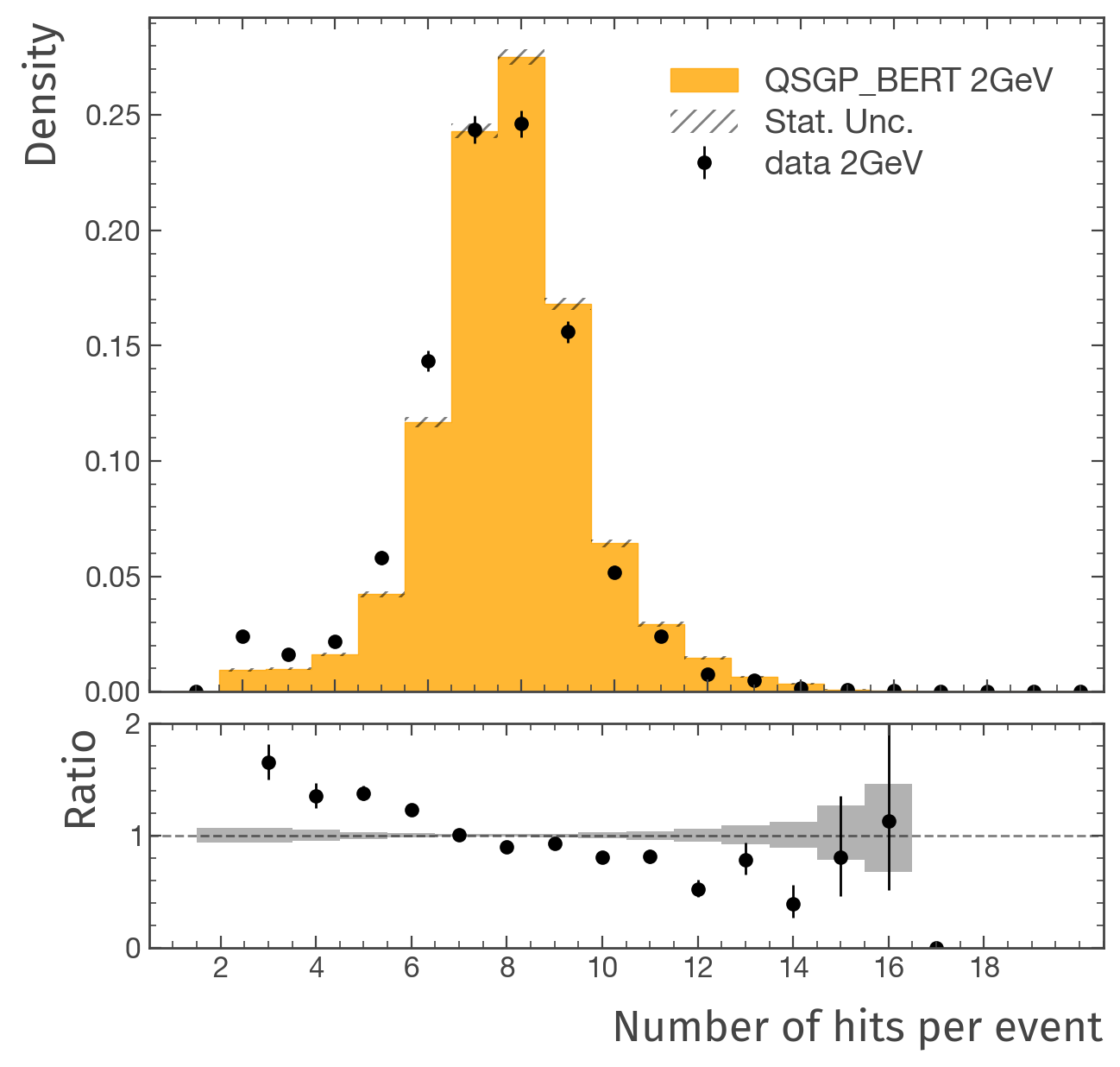
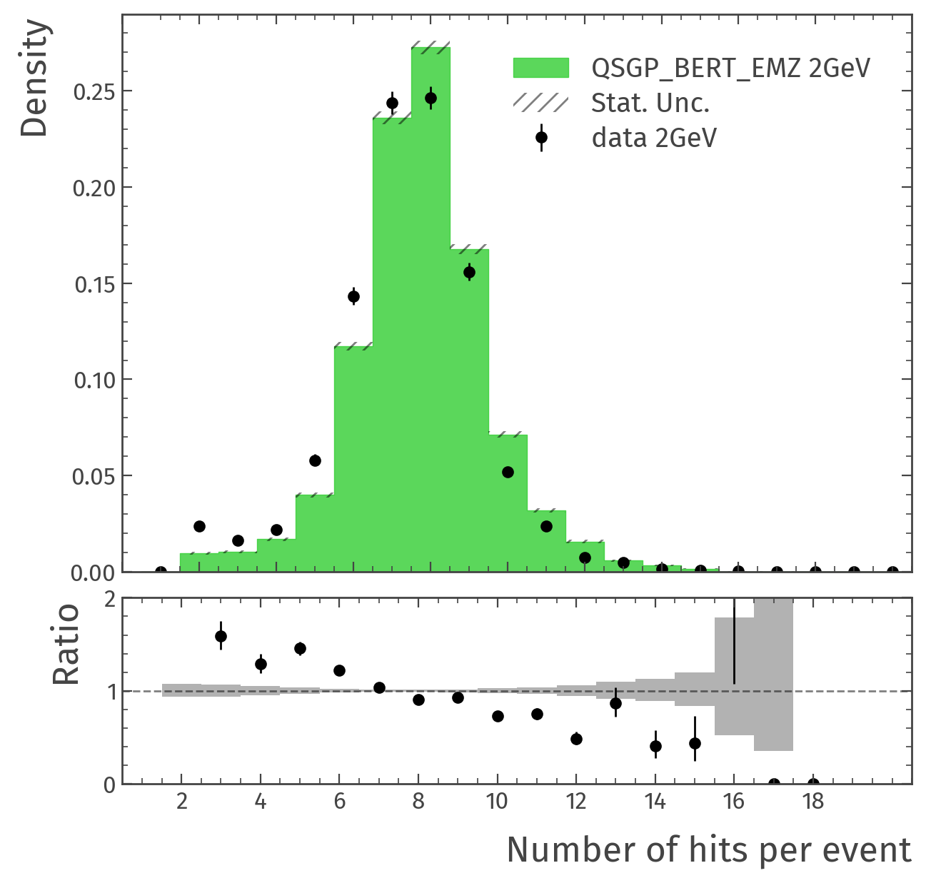
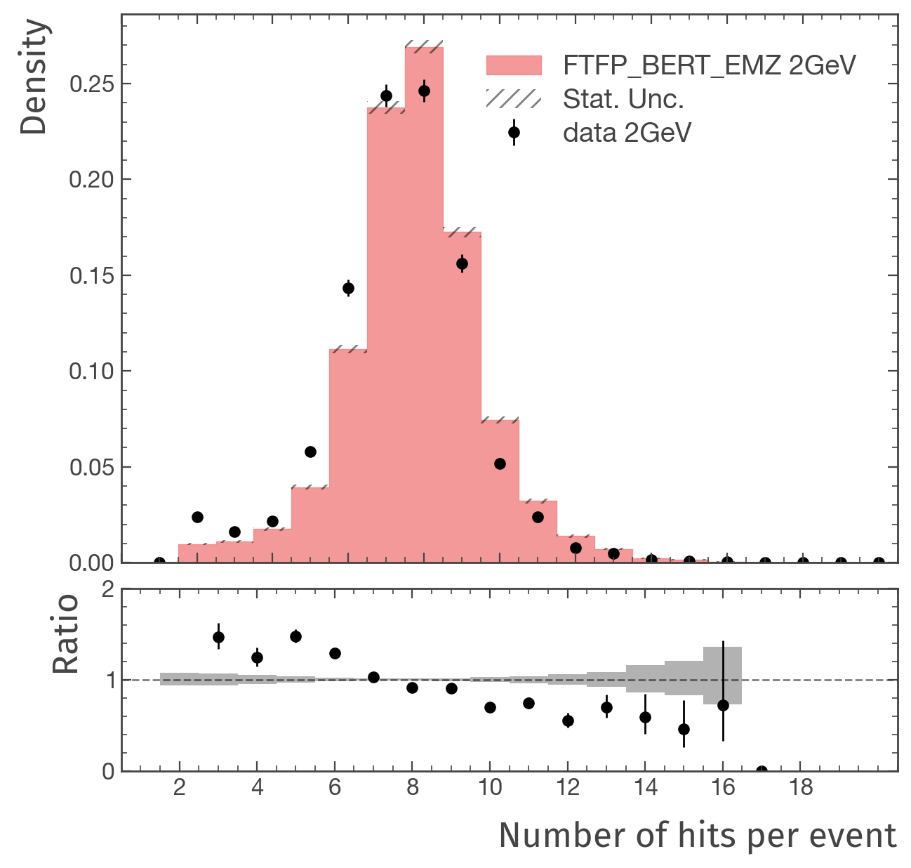
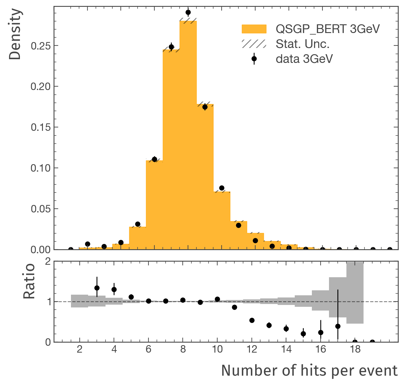
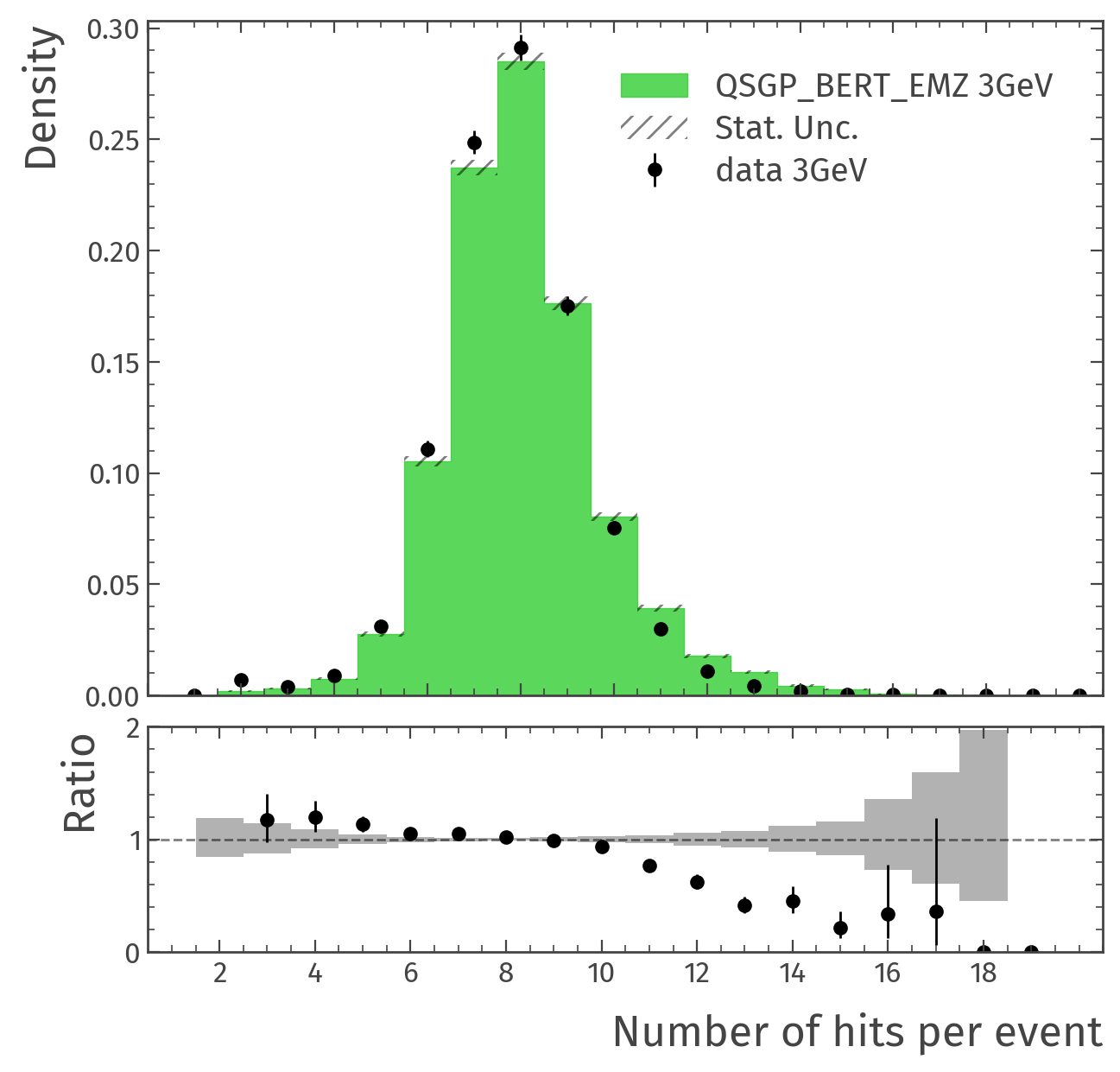
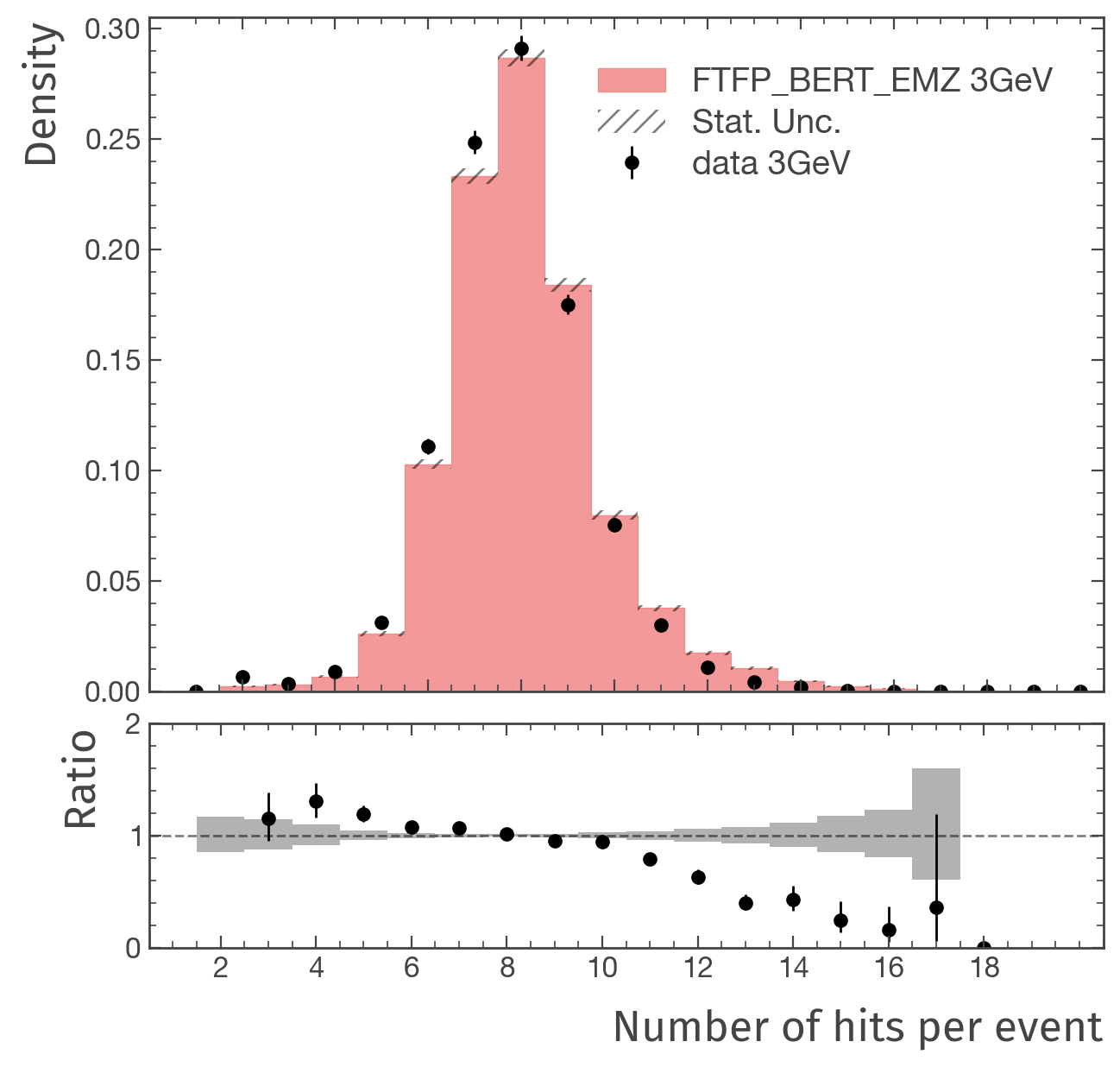
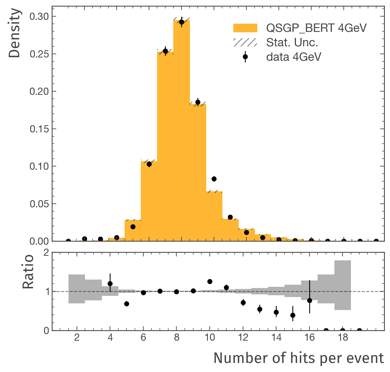
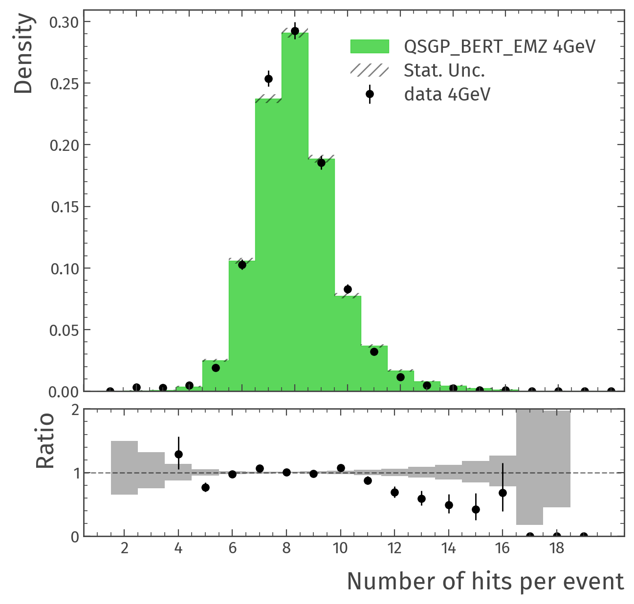
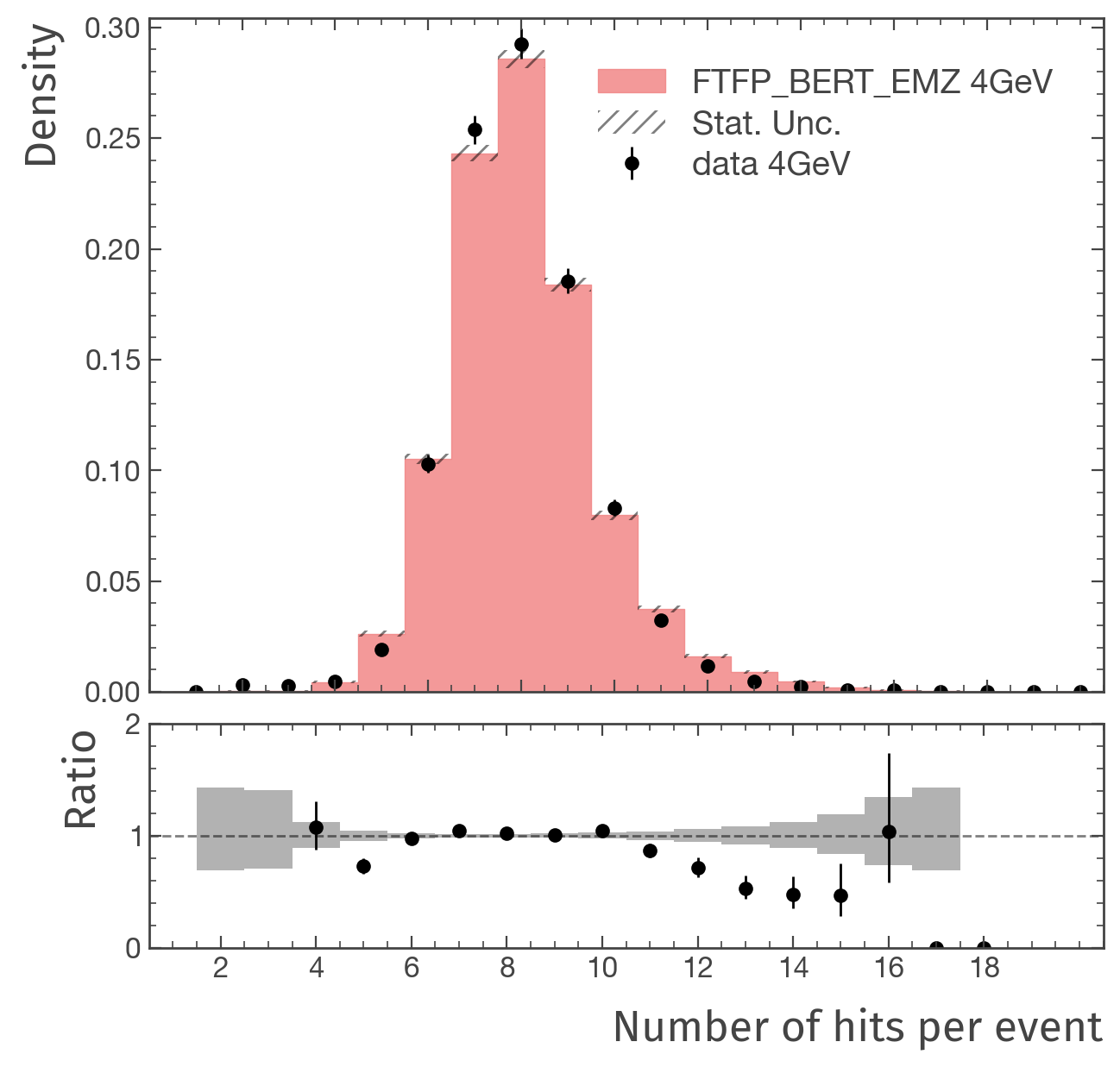
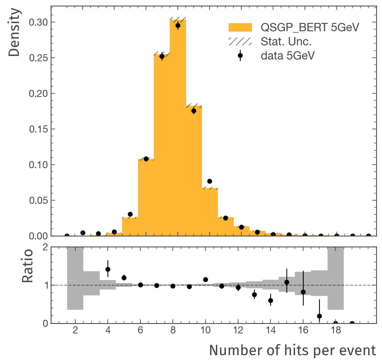
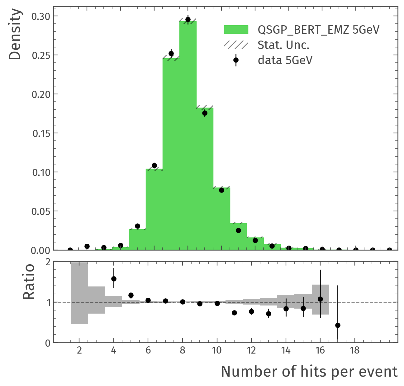
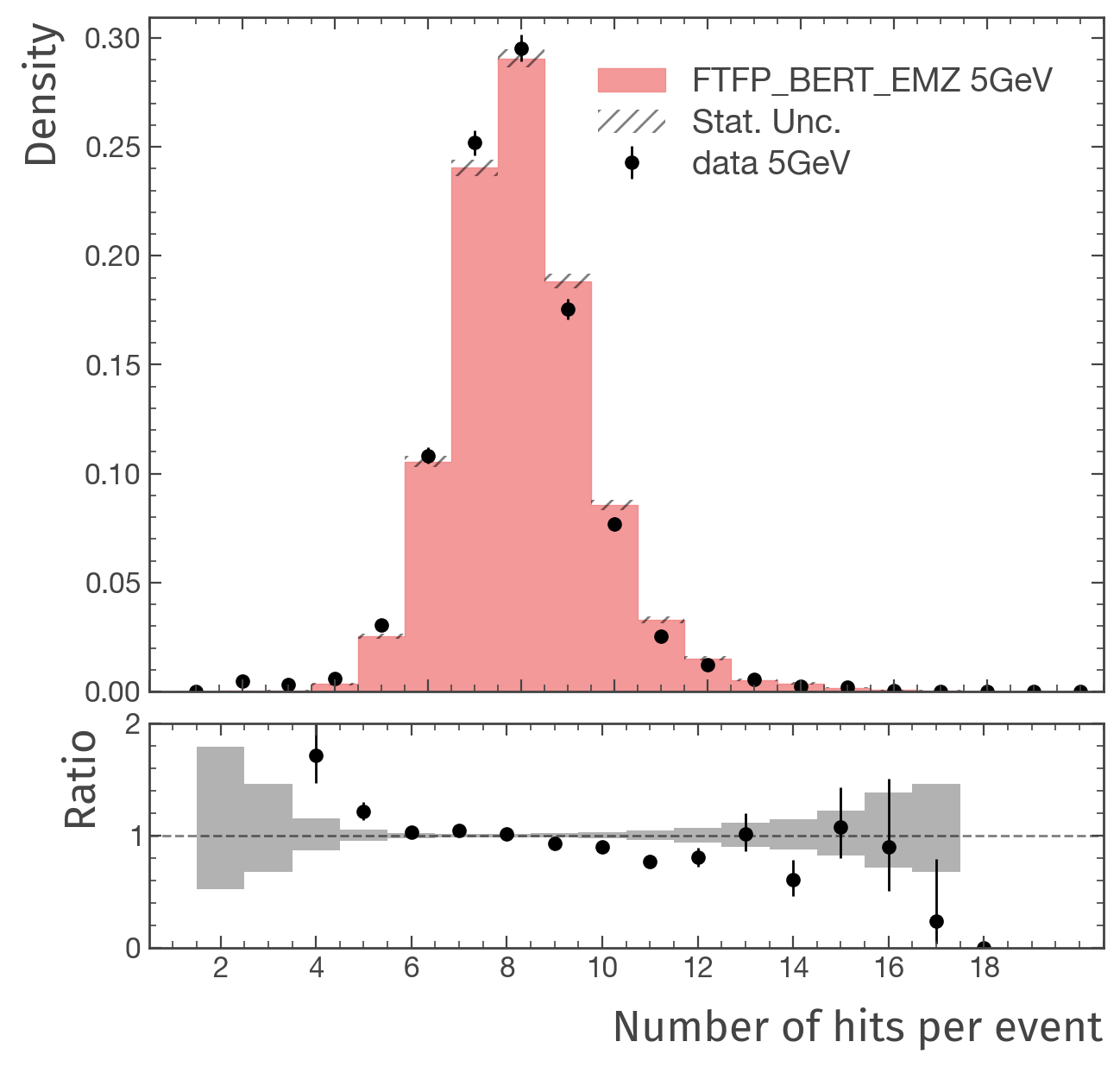
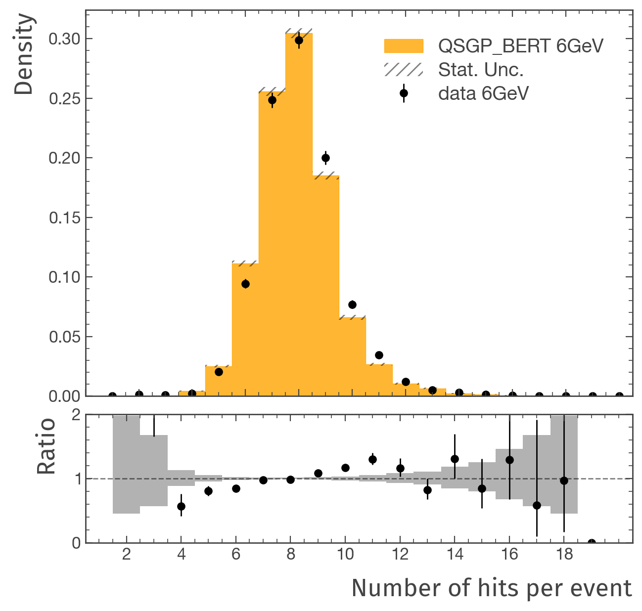
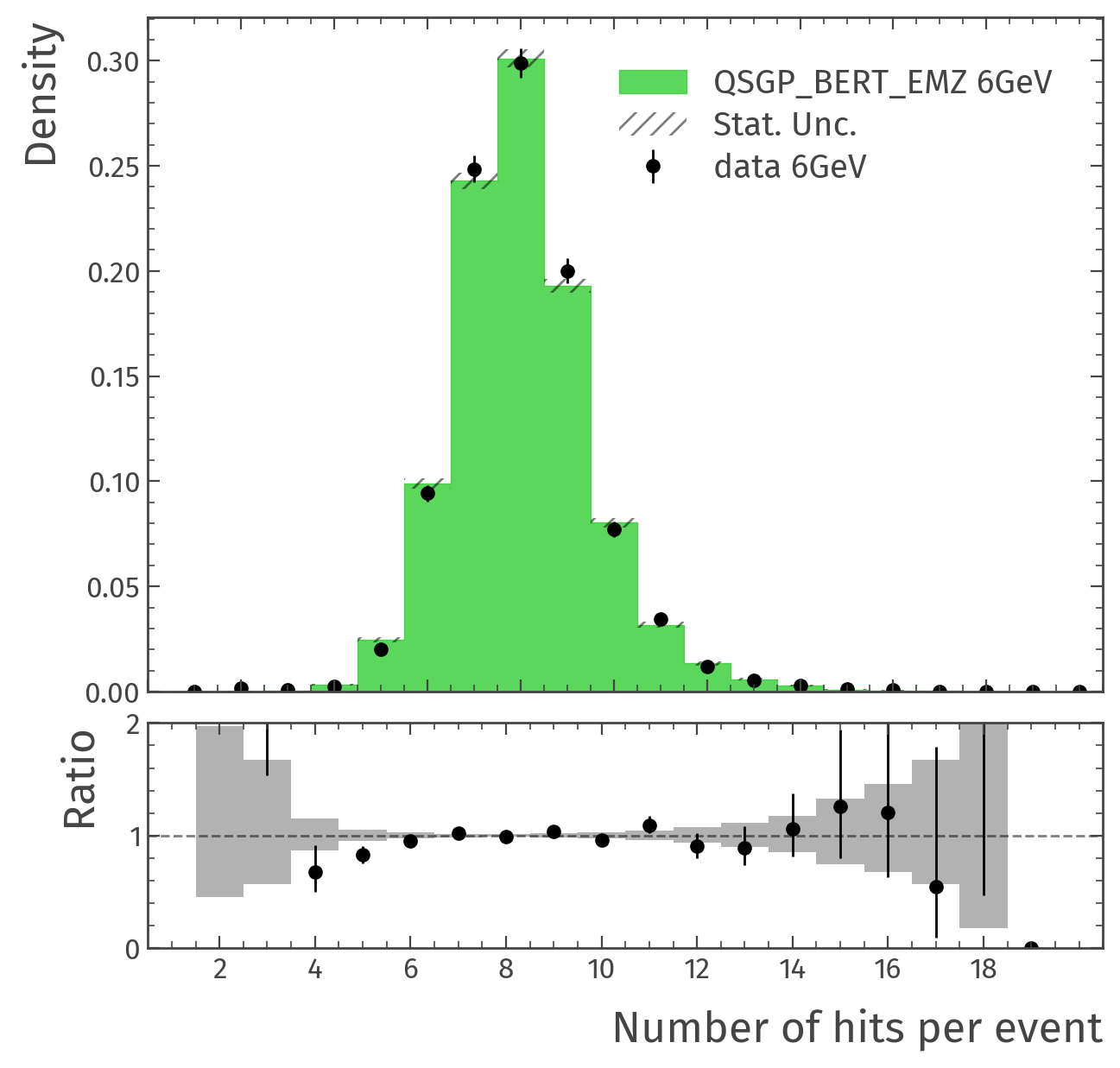
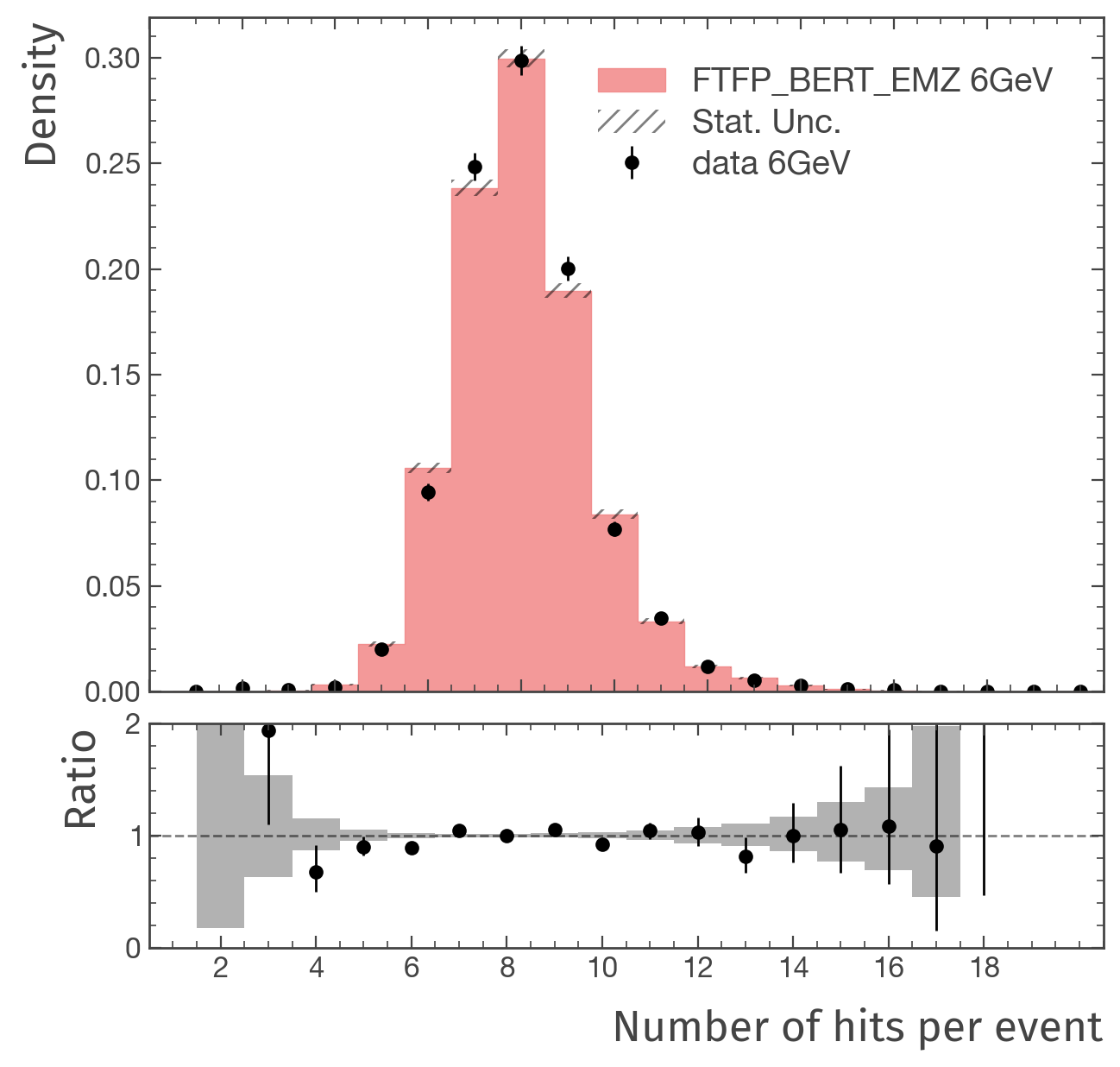
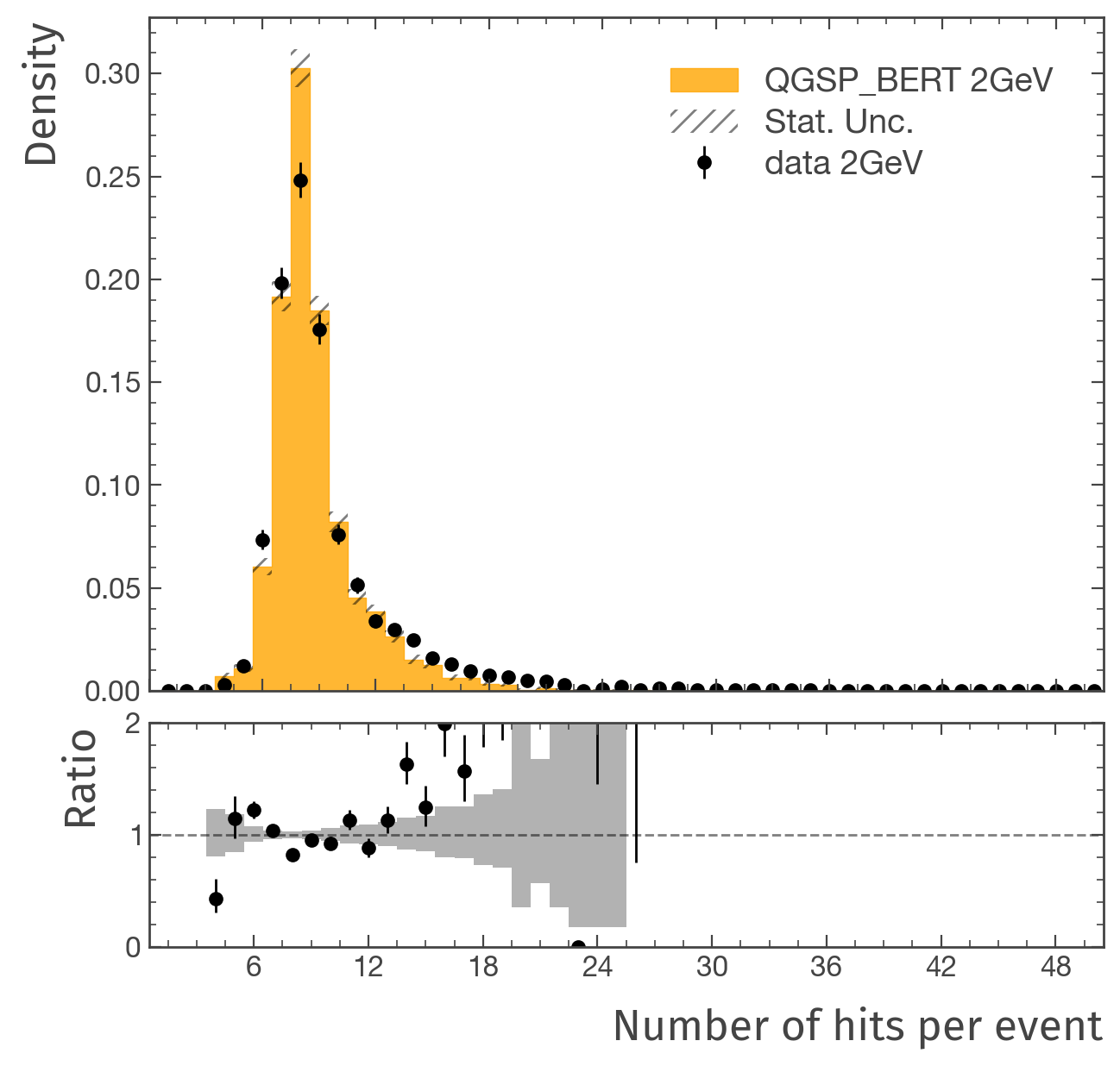
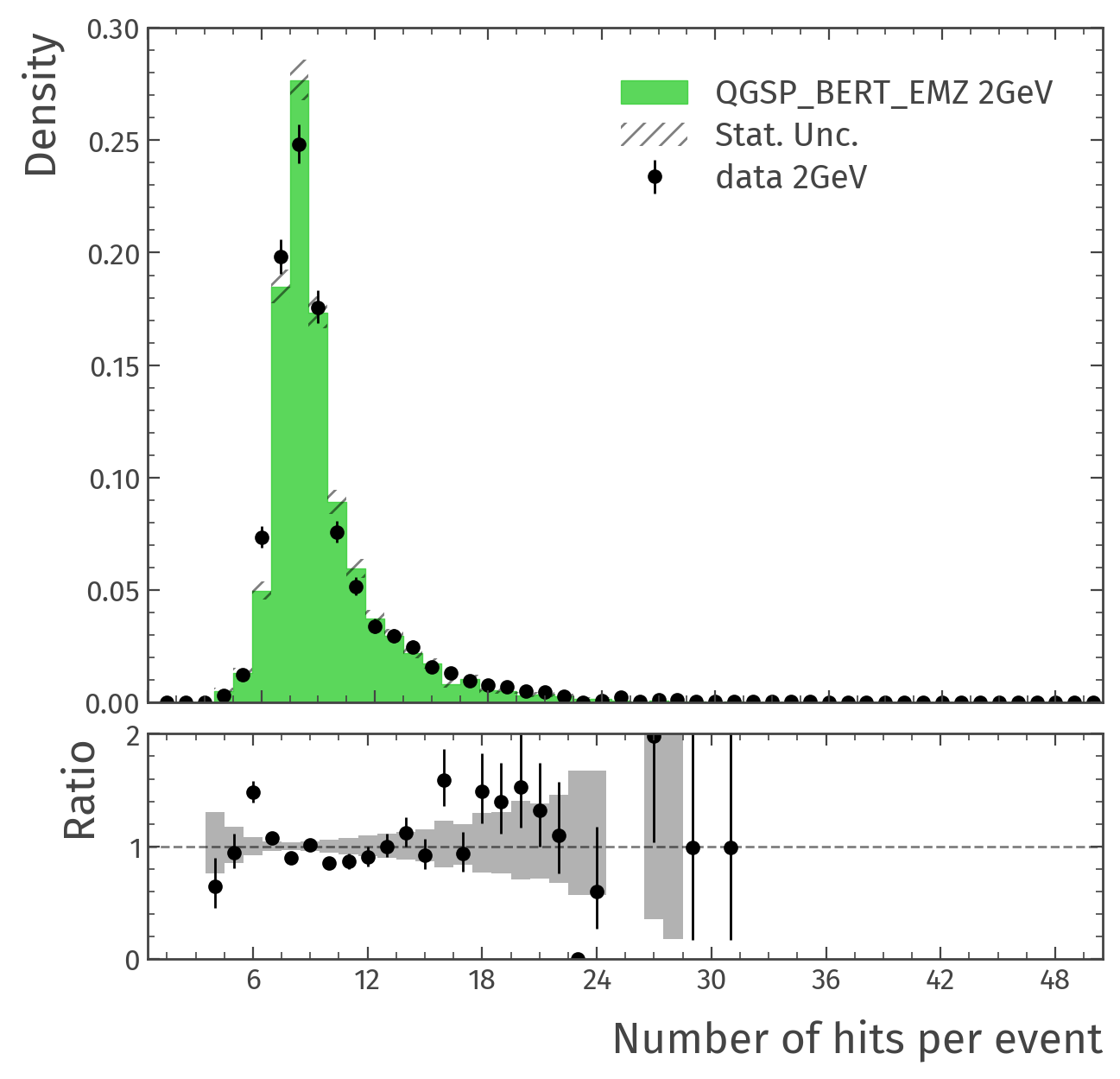
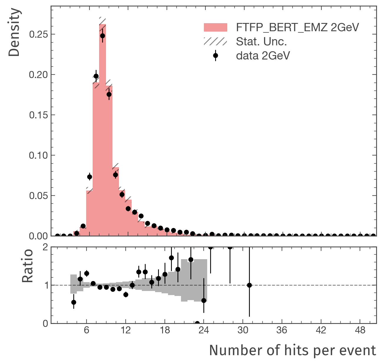
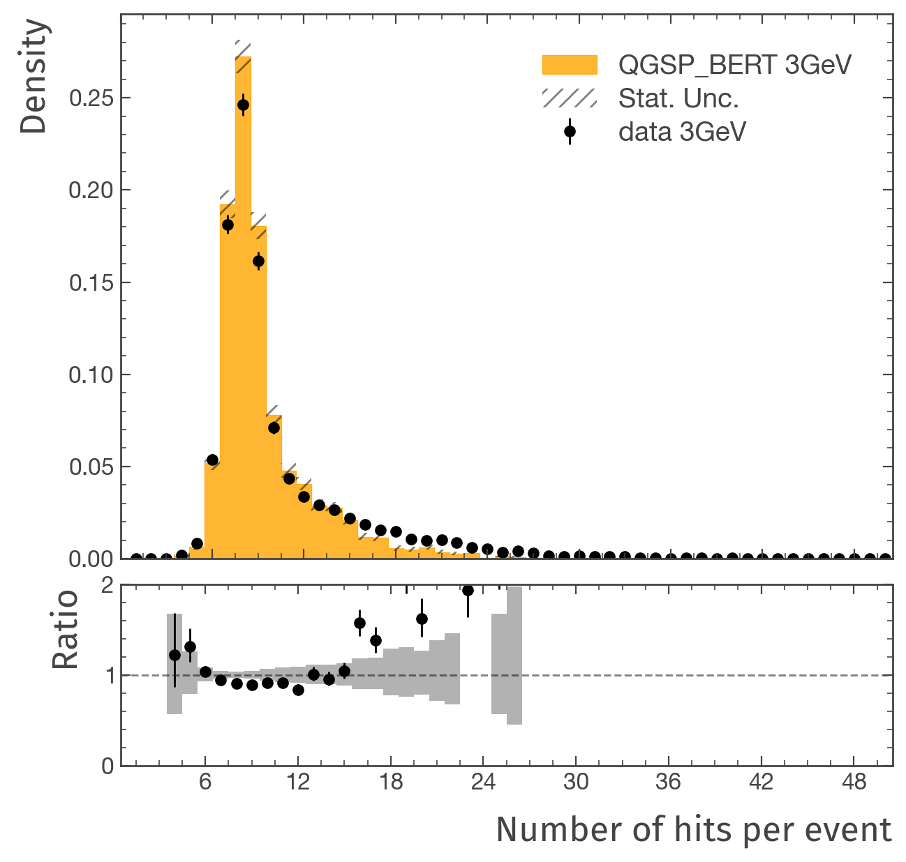
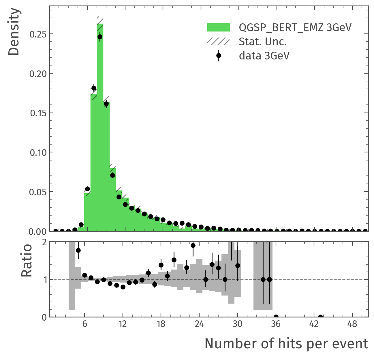
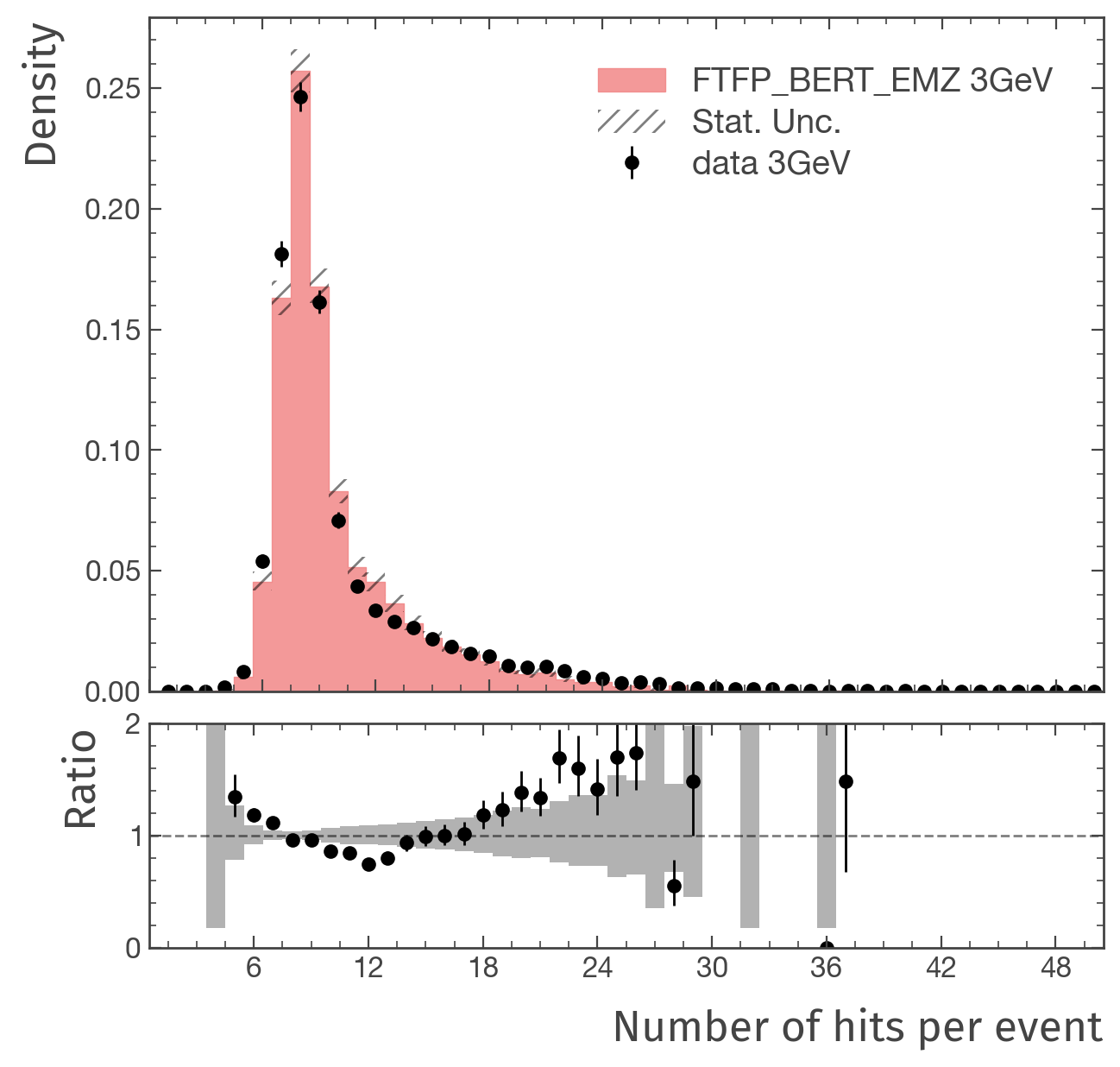
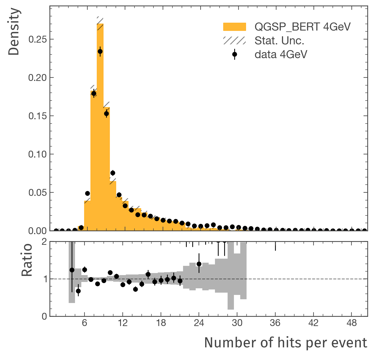
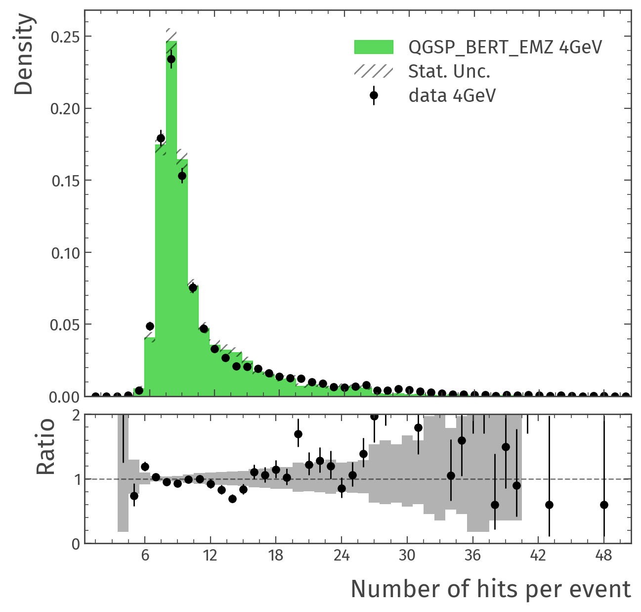
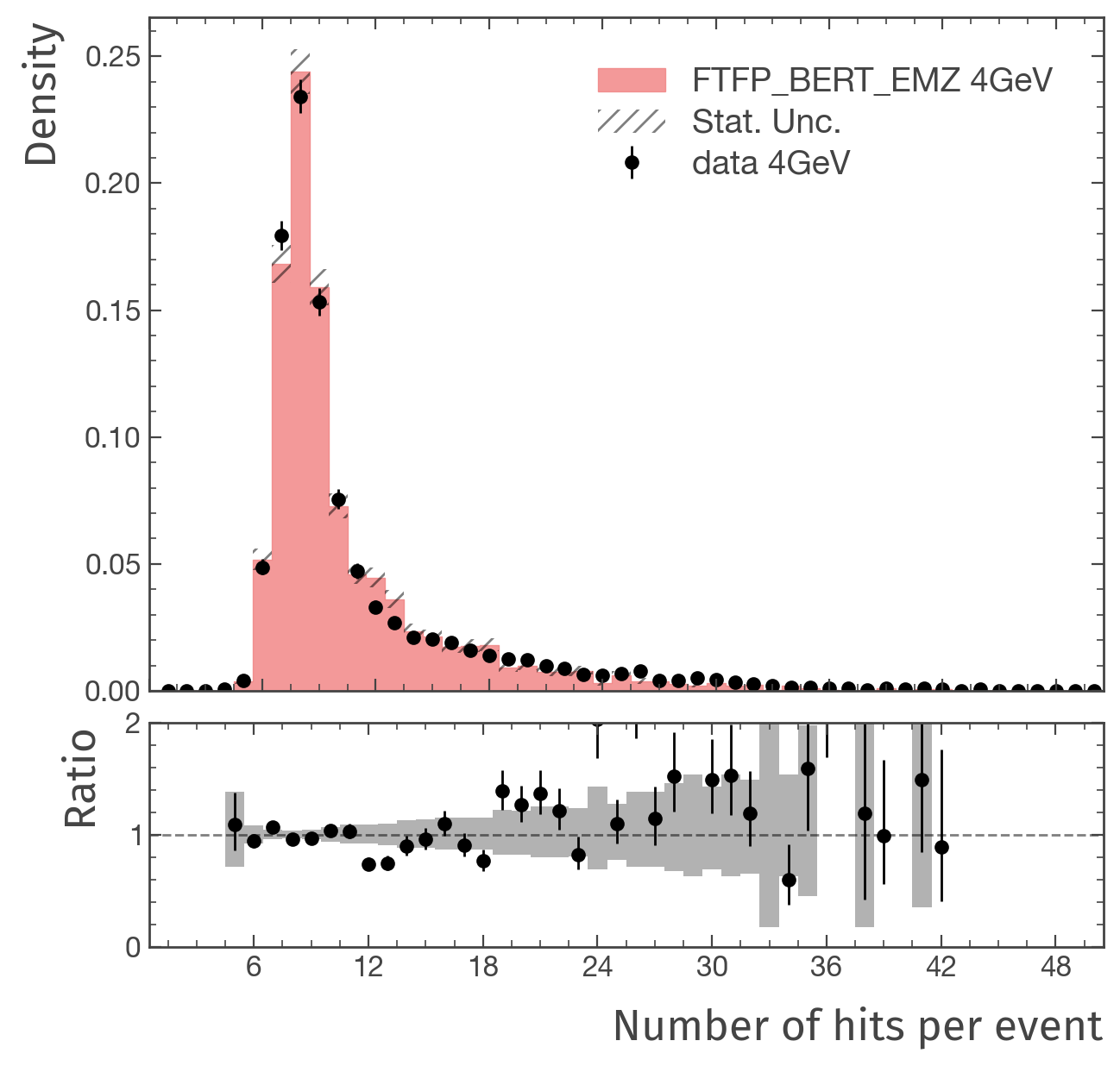
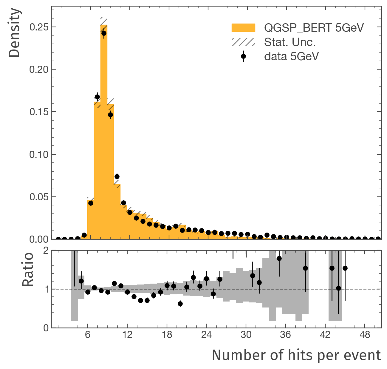
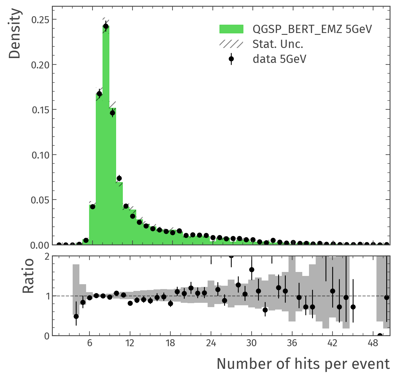
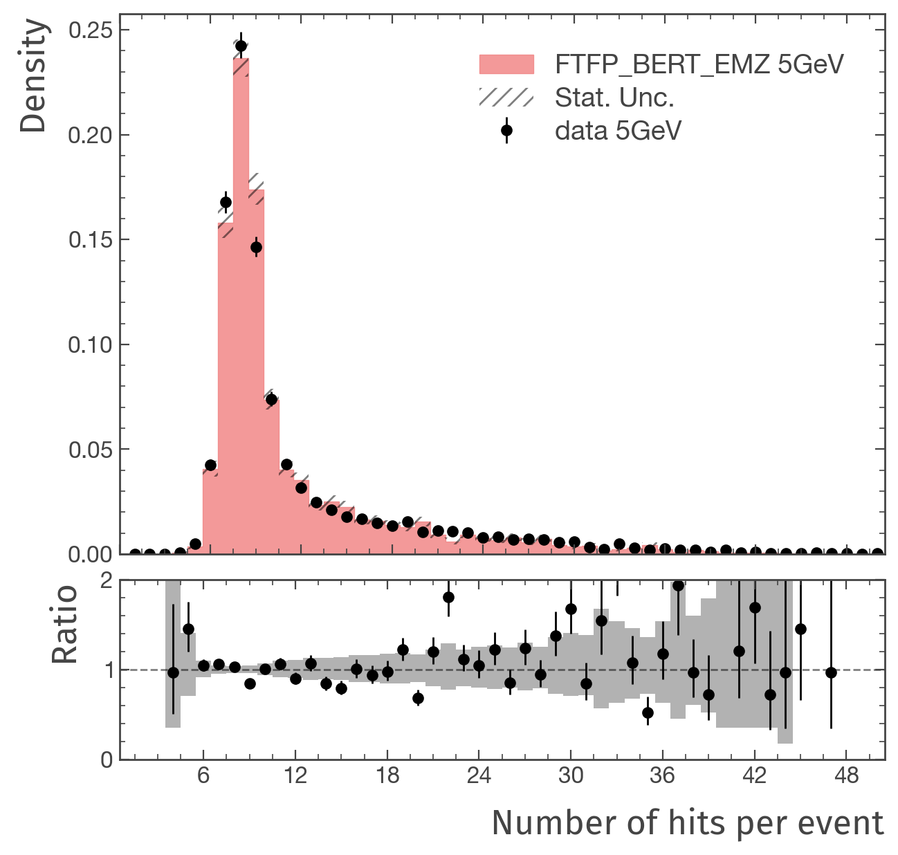
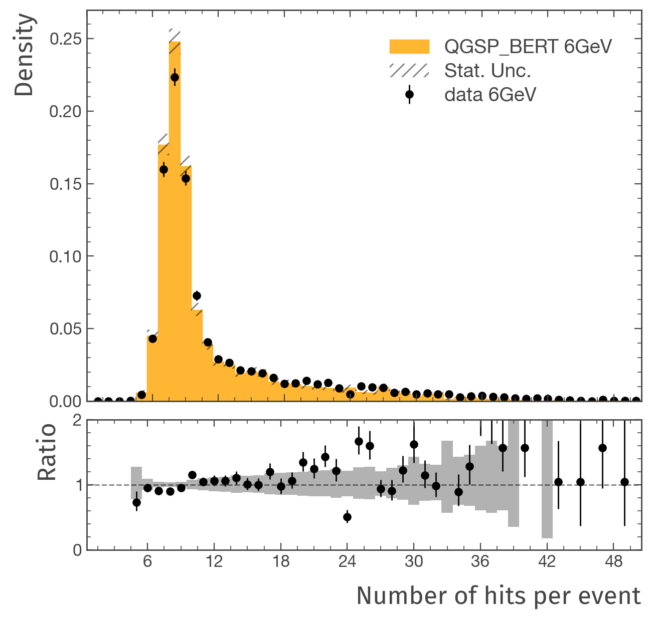
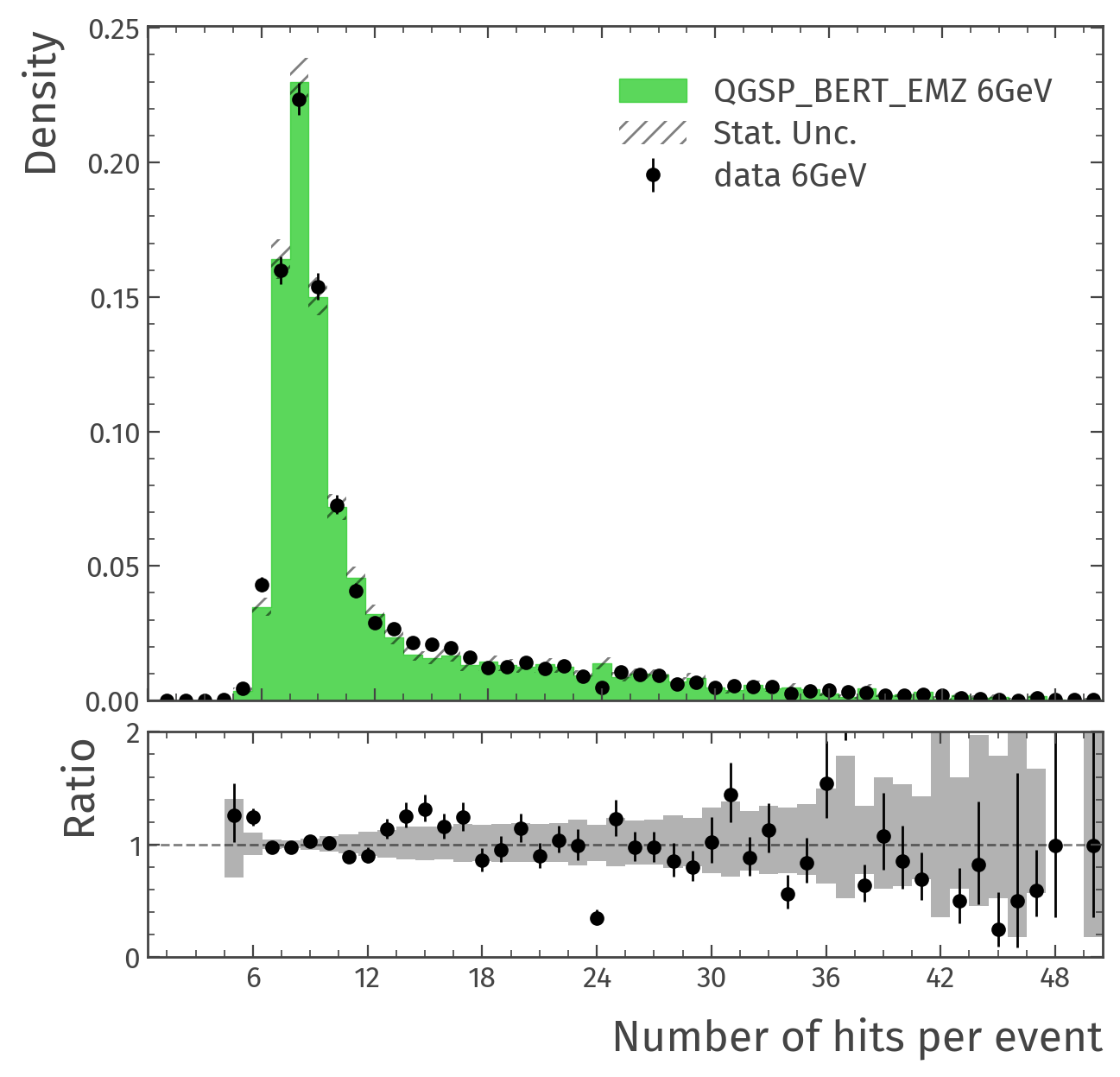
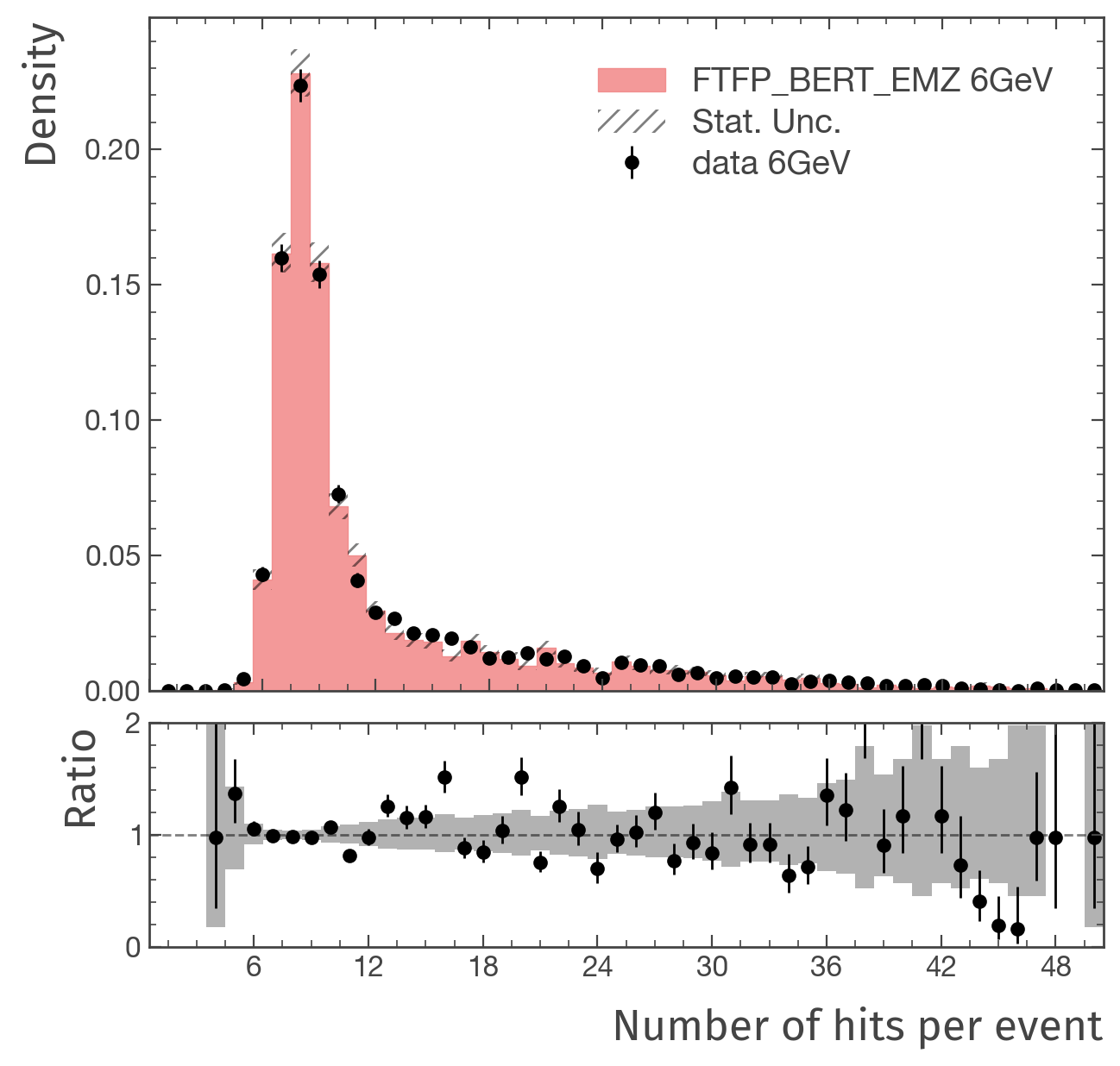
Figure 4 depicts the measured MIP-detection efficiency (left) and the average pad-multiplicity (right) per sampling element using the same estimation method (subsection 2.2) on the test beam data and the simulation. As can be seen, the efficiency and the average pad multiplicity measured in the simulation are in good agreement (within statistical fluctuations) with the experimental measurements. These results conclude the closure test. It confirms that the performance of each simulated sampling element is consistent with the experimental values used to determine its performance in the simulation. Figure 5 shows the distribution of the number of hits per MIP-like event (Figure 3-a) at different pion energies. The black points correspond to the measured data, and the colored regions correspond to the simulation results using the QGSP_BERT (orange), QGSP_BERT_EMZ (green), and FTFP_BERT_EMZ (red) physics lists. Figure 6 shows the distributions for the generic event selection (Figure 3-b). In both event selections, the agreement between the data and the simulation was improved as the beam energy increased. The agreement at the lower energies did not improve when electron impurities were simulated. At the larger number of hits, a better agreement between the data and the simulation is obtained with the physics lists containing the EMZ modeling. For MIP-like events, the distribution peak is expected at eight hits per event – single hit per sampling element. This peak is validated in both event selections at all the tested pion energies and the three physics lists.
4 Simulation Study of 50-layers RPWELL-based DHCAL
Using the presented simulation framework, we modeled a fully-equipped (50 layers) RPWELL-based DHCAL with 2-cm-thick steel absorbers, using the QGSP-BERT-EMZ physics list. These 50 layers correspond to a total depth of 5, inferring a 99.3% chance for a pion to initiate a shower within the module, thus ensuring minimal energy leakage. This depth is consistent with the baseline design HCALs proposed for future collider experiments [2, 3]. We simulated the response of the module to single pions at an energy range of 2–36 GeV, similar to the one tested with the RPC Fe-DHCAL prototype [10]. 50k single pion events were simulated for each energy. The expected performance of the DHCAL was evaluated for different MIP detection efficiencies and pad-multiplicity distributions to study their effect on the pion energy resolution. MIP detection efficiency in the range of 70–98% was considered; based on the efficiency measured with smaller RPWELL prototypes, the high value represents a realistic target. Two pad-multiplicity distributions with average values of 1.1 and 1.6 were tested. The former was measured with a smaller RPWELL sampling element prototype using analog readout at a 150 GeV muon beam [15]. The latter was inspired by the value quoted for the RPC sampling elements [10].
The methodology used for the pion energy reconstruction and the estimation of the pion energy resolution is discussed in subsection 4.1. The results are detailed in subsection 4.2, followed by a discussion in subsection 4.3.
4.1 Simulation Study Methodology
4.1.1 Event Selection
The event selection aims to reduce the energy leakage by considering only pion showers that start in the first ten layers of the calorimeter. This selection relies on identifying the interaction layer – i.e., the first layer in a hadronic shower. Supported by the study of the average longitudinal profile of pion showers that shows an increase in the number of hits per layer across the first three layers of the shower [20], the interaction layer was identified following the methodology presented in [76]. We define each three consecutive layers as a triplet. The average number of hits in the triplet is expressed as , where is the number of hits in the layer. The layer is defined as the interaction layer, if it has more than two hits and is the first layer that fulfills:
Ten layers of the calorimeter are equivalent to about one . In agreement with the expectation, for pion energies of 6–36 GeV, this selection results in 64% efficiency. Pion events of lower energies resulted in lower efficiencies and were excluded from the analysis.
4.1.2 Energy Reconstruction and Uncertainty Calculations
We define the calorimeter response as the relation between the average number of hits per event and the beam energy. Given the observed non-linear response (saturation), a few parametrizations have been proposed. These were not derived from fundamental principles. Two power-law parametrizations were considered in the studies of the RPC-based DHCAL prototypes [20, 77]:
| (4.1) |
| (4.2) |
Here, is the mean value of the Gaussian fit to the distribution of , is the pion beam energy, and , and are free parameters. A positive offset term () sets an energy threshold below which a pion does not yield hits in the calorimeter. The most recent works adapt the parametrization in equation 4.1, in which, on average, hits will be measured in the HCAL for any pion with non-zero energy.
In the context of the MM-based DHCAL studies, a logarithmic parametrization has been used [12]:
| (4.3) |
Reversing the equations above allows expressing the reconstructed energy () as a function of the measured number of hits in an event ():
| (4.4) |
| (4.5) |
| (4.6) |
Using these equations, the energy of each impinging particle is reconstructed from its total number of deposited hits in the calorimeter. For each beam energy, the average reconstructed energy ( ) its associated error (), as well as the width of the distribution () are extracted with a Gaussian fit to the reconstructed energy distribution.
The energy reconstruction bias is defined by the relative difference between and :
| (4.7) |
The relative energy resolution is defined as the ratio between the width of the reconstructed energy distribution over its mean. Its parametrization as a function of the beam energy is:
| (4.8) |
Following [12], the noise term is neglected as the DHCAL threshold is typically set well above the noise level, and the simulation does not include noise.
For simplicity, we refer to the response parametrizations (eqs. 4.1, 4.2, and 4.3) and their corresponding energy reconstruction expressions (eqs. 4.4, 4.5, and 4.6) as the power-law, power-law with an offset, and logarithmic parametrizations.
we estimated the uncertainty of three variables:
-
•
The average number of hits: As mentioned above, for each beam energy, is extracted with a Gaussian fit to the number of hits distribution. Thus, its error is given by:
(4.9) where is the standard deviation of the Gaussian corresponding to a pion beam at energy , and is the number of simulated pions at that specific energy. This is the only error considered when fitting the response parametrizations (eqs. 4.1, 4.2, and 4.3).
-
•
The response function: The uncertainties associated with parameters a, b, and c of the fitted response functions are used to model up and down variations of the response functions.
-
•
The relative energy resolution has two contributions. The first () relates to the uncertainty on the response function and is estimated exploiting its up and down variations. The second () relates to the uncertainty on the mean value of the nominal reconstructed energy distribution (is defined in above). is given by:
(4.10) and are the relative energy resolutions calculated with the nominal response function and its up or down variations, respectively. is obtain from as a standard error propagation and is given by:
(4.11)
Finally, the total up and down uncertainties associated with the nominal relative energy resolution is given by a quadratic sum of and :
| (4.12) |
4.2 Simulation Study Results
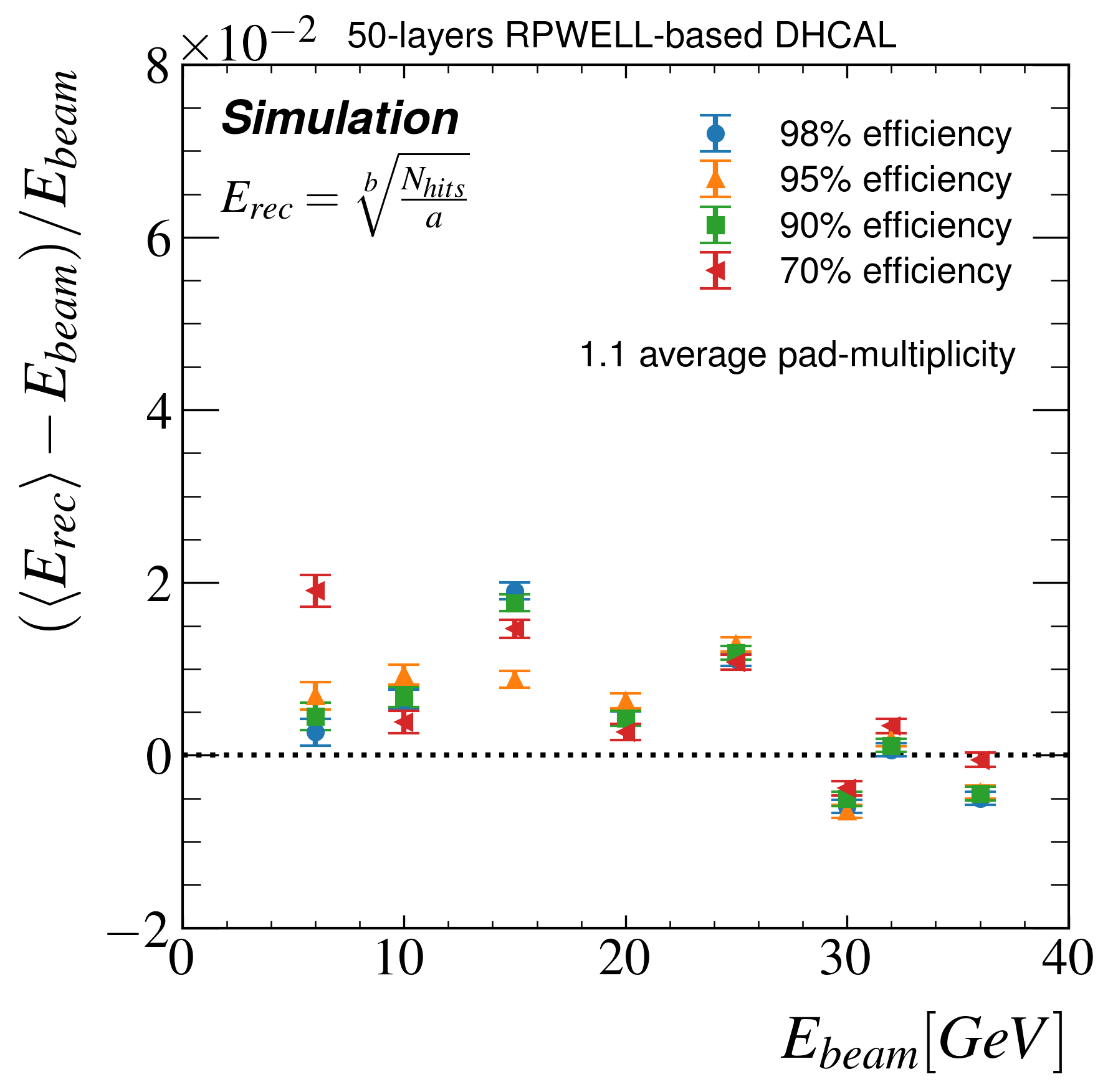
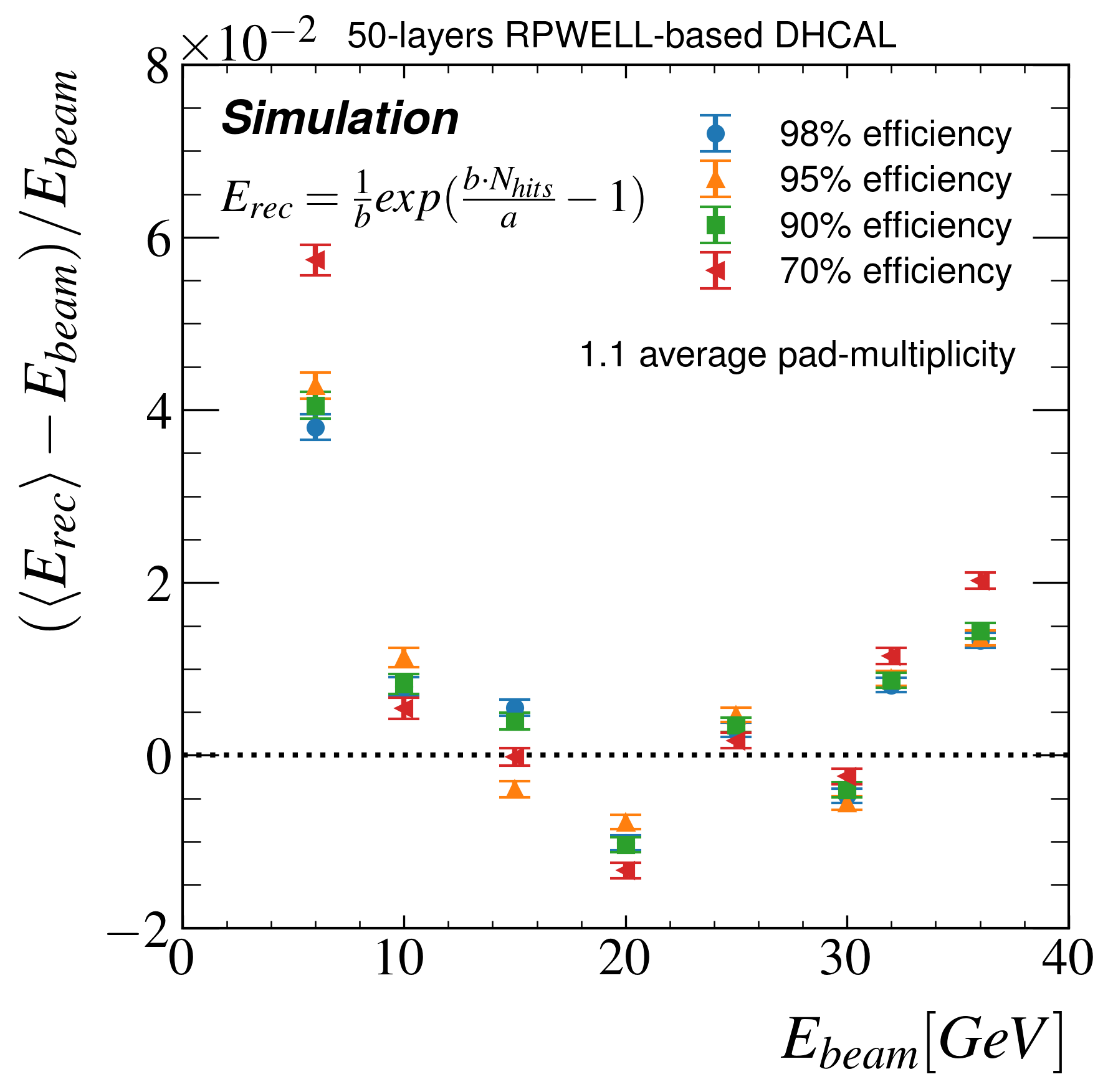
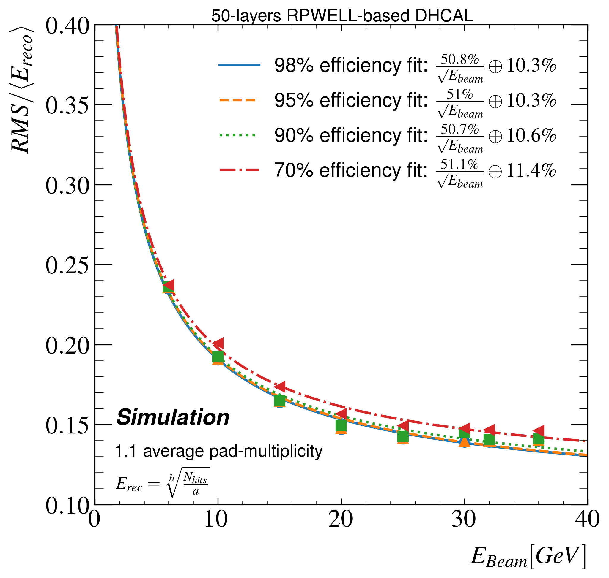
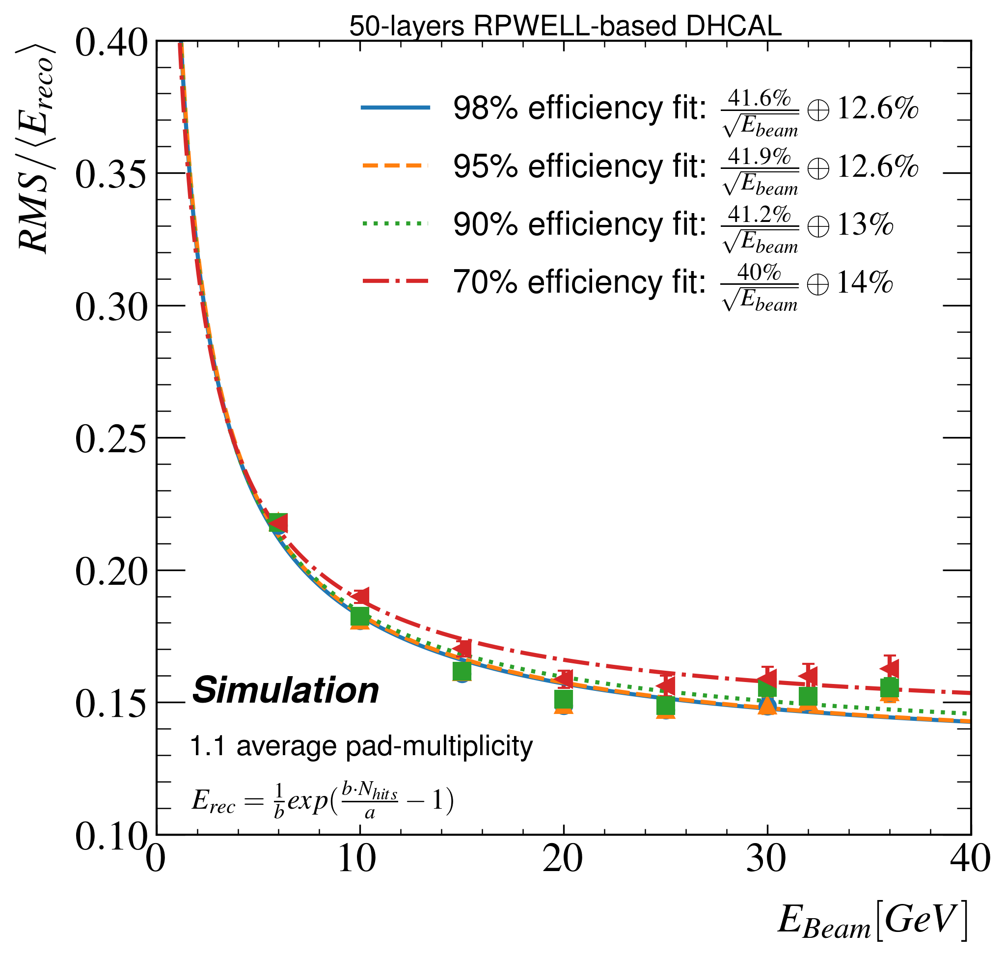
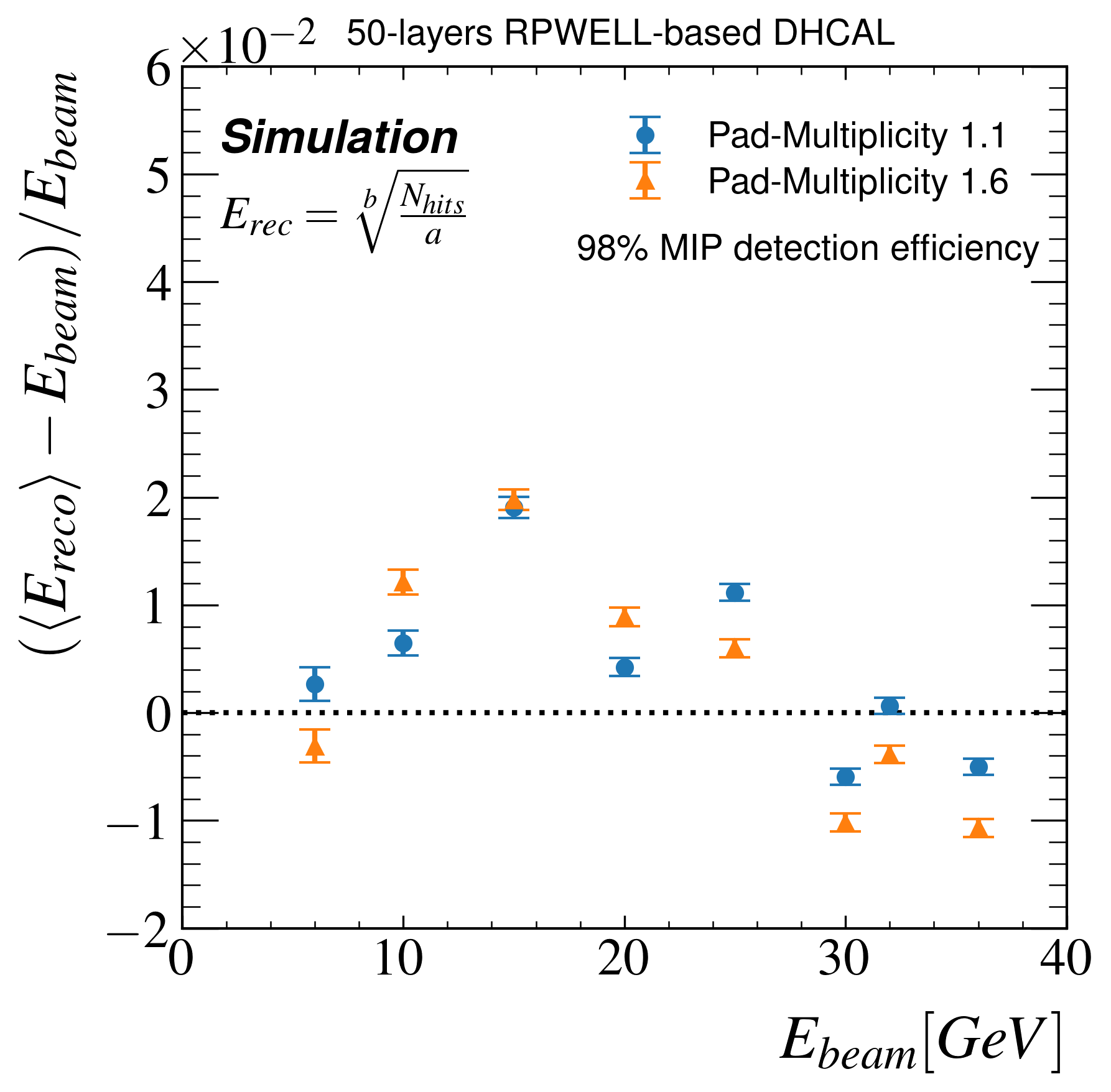
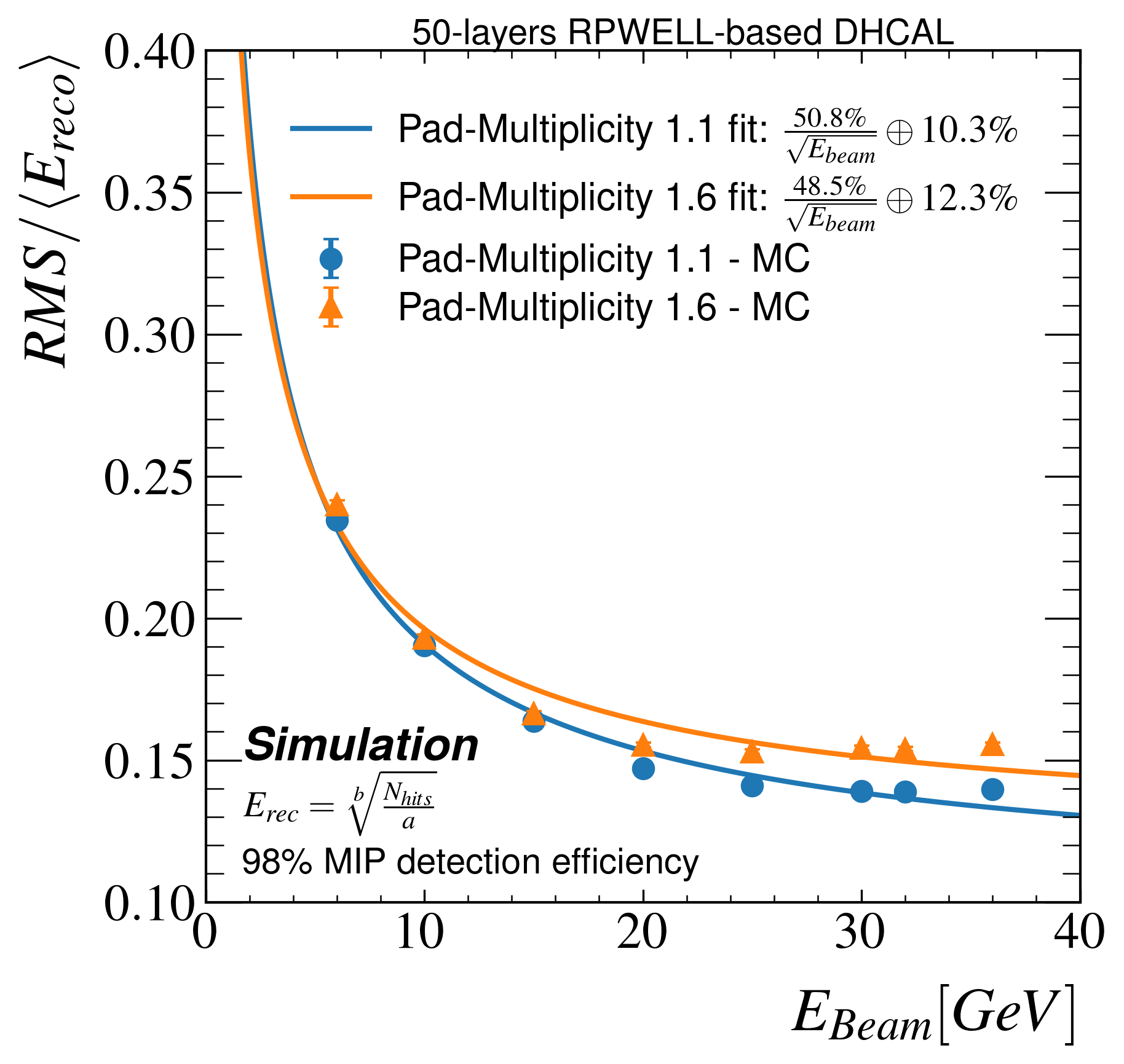
Based on [20], we can target an optimal RPWELL-based DHCAL consisting of sampling elements with 98% MIP detection efficiency and 1.1 average pad-multiplicity. Its calorimeter response is shown in Figure 34 with its three parametrizations; the fit parameters are summarized in Table 4. The energy reconstruction bias and relative energy resolution as a function of the pion beam energy are sown for the three parametrizations in Figure 35 and Figure 36, respectively. The power-law parametrizations yield similar bias values (smaller than 2% with an average of 0.7%), better than those of the logarithmic one (with a maximum bias of 3.5% and an average of 1.2%). The relative energy resolution was obtained with the power-law parametrization, . It is similar to the one of the power-law with an offset, , and superior to that obtained with the logarithmic parametrization, , at pion energies higher than 15 GEV.
We evaluated the effect of the MIP detection efficiency on the DHCAL performance at a fixed pad-multiplicity distribution with an average of 1.1. The calorimeter response for different MIP detection efficiency values is shown in Figure 37 for (a) the power-law, (b) the power-law with an offset, and (c) the logarithmic parametrizations. The fit parameters are summarized in Table 4. Fits of good qualities were obtained as indicated by their corresponding values.


| Parametrization |
|
a | b | c | |||||||||||||||||||||||
|---|---|---|---|---|---|---|---|---|---|---|---|---|---|---|---|---|---|---|---|---|---|---|---|---|---|---|---|
|
|
|
|
|
|||||||||||||||||||||||
|
|
|
|
|
|
||||||||||||||||||||||
|
|
|
|
|
The fit of the power-law with an offset to the calorimeter response yields variations in the offset term for different MIP detection efficiencies without a consistent trend and with substantial uncertainties. It seems that the additional degree of freedom of this parametrization weakens the fit, which might explain why the CALICE collaboration abandoned it. The rest of our analysis concentrates on the reconstruction methods based on the power-law and the logarithmic parametrizations.
Figure 38 shows the bias of the pion energy reconstruction as a function of the beam energy for the (a) power-law and (b) logarithmic parametrizations. The bias measured with the former is smaller than the one measured with the latter, for which large bias is measured at low and high energy values.
Figure 39 presents the relative energy resolution for the different MIP detection efficiency values of the (a) power-law and (b) logarithmic parametrizations. Table 5 lists the fit parameters and their corresponding uncertainties. Comparing the relative energy resolution obtained with the 98% and 70% MIP detection efficiency values, we assess the effects of the MIP detection efficiency. A difference of 0.4% (1.4%) and 1.1% (1.3%) is measured with the power-law (logarithmic) parametrization for the stochastic and constant terms, respectively. This indicates that under the power-law parametrization, the relative energy resolution is less sensitive to uniform changes in the MIP detection efficiency in the tested energy range. Moreover, the relative energy resolution obtained with the power-law parametrization is superior to that obtained with the logarithmic one, as indicated by a 2% smaller constant term.
|
|
S [% GeV] | C [%] | |||||||||||||||||||
|---|---|---|---|---|---|---|---|---|---|---|---|---|---|---|---|---|---|---|---|---|---|---|
|
|
|
|
|
||||||||||||||||||
|
|
|
|
|
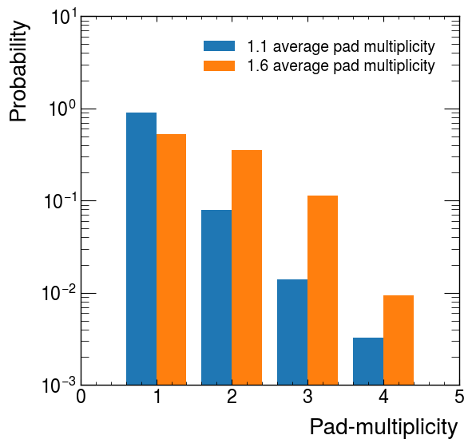
We evaluated the DHCAL performance with two pad-multiplicity distributions (average values of 1.1 and 1.6) at a fixed 98% MIP detection efficiency. The distribution with an average of 1.1 was measured with an RPWELL-based sampling element in a test-beam experiment described in [20]. The average pad-multiplicity of 1.6 was reported for the RPC sampling elements used by the CALICE collaboration [12]. Figure 40 shows the used pad-multiplicity distributions used.
Yielding the best performance in subsection 5.2.2, the power-law parametrization is used in the following. Figure 41 shows the calorimeter response to pions, using the two distributions of pad-multiplicity. The ratio between the average number of hits per event measured with the two distributions is compatible with the ratio of their average values (1.6:1.1). Figure 42 shows their (a) energy reconstruction bias and (b) relative energy resolution. The energy reconstruction bias is similar in both pad-multiplicity distributions, while the relative energy resolution is worse with the higher pad multiplicity.
4.3 discussion
5 Summary
Acknowledgments
We thank Prof. Wang Yi from Tsinghua university in China for kindly providing us with the silicate glass tiles. This research was supported in part by the I-CORE Program of the Planning and Budgeting Committee, the Nella and Leon Benoziyo Center for High Energy Physics at the Weizmann Institute of Science, the common fund of the RD51 collaboration at CERN (the Sampling Calorimetry with Resistive Anode MPGDs, SCREAM, project), Grant No 712482 from the Israeli Science Foundation (ISF), Grant No 5029538 from the Structural Funds, ERDF and ESF, Greece, and the Chateaubriand fellowship from the French Embassy in Israel.
Appendix A Calculation of True Pad-Multiplicity and Hit Detection Efficiency
In subsection 2.2, we mention that the true pad-multiplicity and hit detection efficiency (HDE) can be calculated from the experimental measurements of the distribution of the pad-multiplicity and the MIP detection efficiency. In this appendix, we present a method for an analytic calculation of these parameters. The measured distribution of pad-multiplicity incorporates contributions from both the true pad multiplicity (related to the detector’s response) and from internal multiplicity originating from the interaction of impinging particle with the detector’s material (leaving more than one cluster). Therefore, the calculation consists of two steps:
-
1.
Calculation of the HDE and the distribution of pad-multiplicity before the application of HDE.
-
2.
Calculation of the probability of a hit to have an additional multiplicity due to the impinging particle’s interaction with the detector’s material
A.1 Calculation of the HDE and the pure pad-multiplicity distribution
Let us consider a specific sampling element in the calorimeter. Let and denote the MIP detection efficiency and the measured number of events with pad-multiplicity m, respectively. Both and were measured using the methodology of section 4.1.3. Our goal is to extract the pad’s hit detection efficiency and the true number of events with pad-multiplicity – denoted by and . In short, we would like to get expressions for the following transformation:
The relations can be described as follows:
| (A.1) |
| (A.2) |
The eq. A.2 is a linear combination of the equations derived from eq. A.1, thus, does not contribute to a unique solution. However, we know and the total number of events () which yield an expression for the number of inefficient events ():
| (A.3) |
Assuming that the maximal number of true pad-multiplicity is 4, we need to solve the following equation system:
| (A.4a) | ||||
| (A.4b) | ||||
| (A.4c) | ||||
| (A.4d) | ||||
| (A.4e) | ||||
Solution:
| (A.5a) | ||||
| (A.5b) | ||||
| (A.5c) | ||||
| (A.5d) | ||||
Eq. A.5d is the underlying assumption. We define the parameters ,and in terms of measurable as follows:
| (A.6a) | ||||
| (A.6b) | ||||
| (A.6c) | ||||
| (A.6d) | ||||
And using eqs. A.5 we can express them in term of the true pad-multiplicity and the HDE:
| (A.7a) | ||||
| (A.7b) | ||||
| (A.7c) | ||||
| (A.7d) | ||||
These equations combined with eq. A.5d yield a simple linear equation:
| (A.8) |
Its solution yields the values for , and .
The probability of a hit to have an additional multiplicity due to the detector’s response Let be the number of events with the intrinsic pad-multiplicity that is originating only from the interaction of the beam’s particle and the detector’s material, and be the probability of a hit to have additional pad-multiplicity due to the detector’s response. The following equations express the relations between these parameters:
| (A.9a) | ||||
| (A.9b) | ||||
| (A.9c) | ||||
| (A.9d) | ||||
Thus:
| (A.10a) | ||||
| (A.10b) | ||||
| (A.10c) | ||||
| (A.10d) | ||||
The input parameters that go in to the digitization stage are , and .
References
- [1] M. A. Thomson, Particle-flow calorimetry and the PandoraPFA algorithm, NIM A 611 (2009) 25.
- [2] T. Behnke et al., The International Linear Collider Technical Design Report - Volume 1: Executive Summary (2013) arXiv:1306.6327.
- [3] The CEPC-SPPC Study Group, Volume I - Physics & Detector, CEPC-SPPC: Preliminary Conceptual Design Report (2015) arXiv:1809.00285.
- [4] M. Benedikt, et al., FCC-ee: The Lepton Collider : Future Circular Collider Conceptual Design Report Volume 2, EPJ Spec. Top. 228 (2019) 261-623.
- [5] L. Linssen, et al., Physics and Detectors at CLIC: CLIC Conceptual Design Report (2012) arXiv:1202.5940.
- [6] F. Felix Sefkow, Experimental Tests of Particle Flow Calorimetry, Rev. Mod. Phys. 88 (2016) American Physical Society, 015003.
- [7] S. Mannai, et al., High granularity Semi-Digital Hadronic Calorimeter using GRPCs, NIM A 718 (2013) 91.
- [8] J. Repond, Analysis of DHCAL Muon Events, in TIPP 2011 Conf. Chicago 4, (2011).
- [9] CALICE Collaboration, et al., First results of the CALICE SDHCAL technological prototype, JINST 11 IOP Publishing, (2016) P04001.
- [10] CALICE Collaboration, Analysis of Testbeam Data of the Highly Granular RPC-Steel CALICE Digital Hadron Calorimeter and Validation of Geant4 Monte Carlo Models, NIM A 939 (2019) 89-105.
- [11] C. Adloff, et al., Construction and test of a 1×1 m 2 Micromegas chamber for sampling hadron calorimetry at future lepton colliders, NIM A, (2013).
- [12] M. Chefdeville, Micromegas for Particle-flow Calorimetry, Proceedings, Int. Conf. CHEF 2013 Paris, Fr. (2013).
- [13] D. Hong, et al., Development of compact micro-pattern gaseous detectors for the CEPC digital hadron calorimeter, JINST. 15, IOP Publishing, (2020) C09032.
- [14] D. Hong, et al. Update of the 100cm×50cm RWELL detector for DHCAL application in RD51 Collaboration Meeting and Topical Workshop on FE electronics for gas detectors, November 2021.
- [15] L. Moleri, et al., In-beam evaluation of a medium-size Resistive-Plate WELL gaseous particle detector, JINST 11, IOP Publishing, (2016) P09013.
- [16] C. Adloff, et al., Resistive Micromegas for Sampling Calorimetry PoS 054, in TIPP, (2014).
- [17] S. Bressler, et al., First in-beam studies of a Resistive-Plate WELL gaseous multiplier, JINST 11, (2016) P01005.
- [18] L. Moleri, et al., On the localization properties of an RPWELL gas-avalanche detector, JINST 12, (2017) P10017.
- [19] P. Bhattacharya, L. Moleri and S. Bressler, Signal formation in THGEM-like detectors, NIM A (2019).
- [20] L. Moleri, et al., The Resistive-Plate WELL with Argon mixtures – A robust gaseous radiation detector, NIM A 845 (2017) 262.
- [21] S. Bressler, et al., Novel Resistive-Plate WELL sampling element for (S)DHCAL, NIM A 958 (2020).
- [22] D. Shaked Renous, et al., Towards MPGD-Based (S)DHCAL, J. Phys. Conf. Ser. 1498, IOP Publishing, (2020).
- [23] M. Alexeev, et al., The gain in Thick GEM multipliers and its time-evolution, JINT 10, IOP Publishing, (2015) P03026.
- [24] C. Adloff, et al., MICROROC: MICRO-mesh gaseous structure Read-Out Chip, JINST. 7, (2012) C01029.
- [25] R. O. Duda and P. E. Hart, Use of the Hough Transformation to Detect Lines and Curves in Pictures, Commun. ACM 15, ACM PUB27 New York, NY, USA , (1972) 11.
- [26] S. Agostinelli, et al., GEANT4 - A simulation toolkit, NIM A. 506 (2003) 250.
- [27] J. Apostolakis, et al., GEANT4 Physics Lists for HEP, IEEE Nucl. Sci. Symp. Conf. Rec. (2008).
- [28] Electromagnetic physics constructors — PhysicsListGuide 10.7 documentation https://geant4-userdoc.web.cern.ch/UsersGuides/PhysicsListGuide/html/electromagnetic/index.html (14 May 2021).