Mixtures of Gaussian Process Experts with SMC²

Abstract

Gaussian processes are a key component of many flexible statistical and machine learning models. However, they exhibit cubic computational complexity and high memory constraints due to the need of inverting and storing a full covariance matrix. To circumvent this, mixtures of Gaussian process experts have been considered where data points are assigned to independent experts, reducing the complexity by allowing inference based on smaller, local covariance matrices. Moreover, mixtures of Gaussian process experts substantially enrich the model’s flexibility, allowing for behaviors such as non-stationarity, heteroscedasticity, and discontinuities. In this work, we construct a novel inference approach based on nested sequential Monte Carlo samplers to simultaneously infer both the gating network and Gaussian process expert parameters. This greatly improves inference compared to importance sampling, particularly in settings when a stationary Gaussian process is inappropriate, while still being thoroughly parallelizable.

Keywords: sequential Monte Carlo, SMC², Gaussian processes, mixture of experts, classification

1 Introduction

Gaussian processes (GP) are a versatile tool for statistical modelling of data where the exact form of the mapping between input and output variables is unknown and have found a plethora of applications. Recent applications of GPs include prediction of battery life times (Richardson et al., 2017), geometry optimization in theoretical chemistry (Denzel and Kästner, 2018), spectral peak structure prediction (Wakabayashi et al., 2018), tokamak plasma modelling (Ho et al., 2019), medical diagnosis using proteomic data (Yu et al., 2022), and pile foundation design (Momeni et al., 2020), just to name a few.

However, straight-forward application of GPs suffers from cubic computational complexity and memory constraints due to the need of inverting and storing a full covariance matrix of size $N\times N$ for $N$ data points. Moreover, many applications present departures from the standard GP model, such as non-stationary, heteroscedasticity, and non-normality. To overcome these limitations, mixtures of GP experts have been considered (e.g. Tresp, 2001; Rasmussen and Ghahramani, 2002; Meeds and Osindero, 2005).

Mixtures of GP experts belong to the general class of mixtures of experts (MoEs) (see Masoudnia and Ebrahimpour, 2014; Gormley and Frühwirth-Schnatter, 2019, for reviews). The nomenclature has it origins in machine learning (Jordan and Jacobs, 1994), but they appear in many different contexts such as in statistics, where they are often called dependent mixtures (MacEachern et al., 1999; Quintana et al., 2022) and econometrics where they are referred to as smooth mixtures (Li et al., 2011; Norets, 2010; Villani et al., 2012). MoEs probabilistically partition the input space into regions and specify a local expert within each region. The gating network maps the experts to local regions of the input space, determining the partition of the data into independent sets. Local experts are fit independently to the data sets, where each expert is a conditional model for the output $y$ given the input $x$, which is specifically a GP model in the case of mixtures of GP experts. This allows for both improved scalability, as each GP expert fit only requires inversion and storing of the local covariance matrices, and flexibility, as GP experts can capture different behaviors, e.g. smoothness and variability, within each region.

Inference for mixtures of GP experts is often performed via Markov chain Monte Carlo (MCMC), namely, Gibbs sampling (Meeds and Osindero, 2005; Rasmussen and Ghahramani, 2002; Gadd et al., 2020), by augmenting the model with a set of latent allocation variables denoting the labels of the expert associated to each data point. This provides asymptotically exact samples from the posterior, however it often comes with a high computational cost due to slow mixing and long convergence times. For faster approximate inference, Yuan and Neubauer (2008) develop a variational inference scheme, and Tresp (2001) employs an expectation-maximization algorithm for maximum a posteriori (MAP) inference. A combination of variational inference, MAP, and sparse GPs (Quinonero-Candela and Rasmussen, 2005) is developed in Nguyen and Bonilla (2014) to improve scalability to big data (e.g. training size of $10^{5}$), and this is further expanded upon in Etienam et al. (2020) for fast one-pass approximate MAP inference.

Recently, Zhang and Williamson (2019) proposed an embarrassingly parallel approach for mixtures of GP experts based on importance sampling. Importantly, this allows for uncertainty quantification in the parameters and quantities, as opposed to MAP inference, and avoids the independence or distributional assumptions of variational inference. Moreover, in the proposal distribution, random partitions of the data points are generated, allowing for easily distributed GP likelihood computation. However, it is well known that naive importance sampling requires the number of importance samples to be exponential in the the Kullback-Liebler (KL) divergence of the posterior from the proposal distribution (Chatterjee and Diaconis, 2018). We discuss how this number can be quite large for mixtures of GP experts due to the massive number of possible partitions, leading to poor inference, particularly when a stationary GP model is inappropriate.

To address this, we propose to improve upon the approach of Zhang and Williamson (2019) by using nested sequential Monte Carlo (SMC) samplers, as introduced by Chopin et al. (2013), as a way of inferring the model parameters from the posterior. We discuss and demonstrate how this provides a more accurate and robust approach, especially for complex target distributions resulting from complex behaviors of the data, such as non-stationarity, discontinuities, or heterogeneity. Furthermore, for complex target distributions our method can be much more computationally more efficient, while still being thoroughly parallelizable. It is well-known that SMC methods reduce importance sampling complexity from exponential to polynomial (Beskos et al., 2014). Some parallelizability must be sacrificed due to weight normalization, but all other stages of the algorithm can be executed independently and in parallel. If more parallel capacity is available and more resources are required, then parallel SMCs can also be run, provided that a minimum ensemble size is used for each one, see e.g. Jasra et al. (2020). It is worth noting that several studies have previously proposed using SMC in various different ways to sample from standard mixture models, such as Bouchard-Côté et al. (2017) for split-merge moves, amongst other approaches (MacEachern et al., 1999; Fearnhead, 2004; Fearnhead and Meligkotsidou, 2007; Mansinghka et al., 2007; Caron and Doucet, 2009; Carvalho et al., 2010; Ulker et al., 2010).

In summary, we formulate mixtures of GP experts such that nested SMC samplers can be used. The nested SMC samplers, or SMC², allow for separation of the model inference into two separate parts, the sampling of the gating network parameters and GP parameters. We highlight that this allows for incorporation of uncertainty in the GP parameters, in contrast to the MAP estimates employed in Zhang and Williamson (2019). The use of SMC² greatly extends the set of feasible target posterior distributions from the previously proposed embarrassingly parallel importance sampling of mixtures of GP experts.

The rest of the paper is organized as follows. We formulate the statistical model in Section 2, which is followed by a review of importance sampling in Section 3 and a description of the proposed SMC² sampler in Section 4. In Section 5, we provide our construction of the predictive distribution, and results are presented for various numerical examples in Section 6. We conclude with final remarks and a discussion in Section 7.

2 Model

In a supervised setting, MoEs provide a flexible framework for modelling the conditional relationship between the outputs $y$ given the inputs $x$, and two general approaches exist for defining MoEs, namely, generative and discriminative. Generative MoEs model $(y,x)$ jointly, while discriminative MoEs model the conditional of interest directly. In this work, we focus on the discriminative approach, which has the advantage of avoiding modelling of and placing any distributional assumptions on the input variables.

We assume that the data consists of a sample of size $N$ input variables $X=\{x_{1},\dots,x_{N}\}$, with $x_{i}=(x_{i,1},\dots,x_{i,D})$, and output variables $Y=\{y_{1},\dots,y_{N}\}$. For simplicity, we focus on the case when $x_{i}\in\mathbb{R}^{D}$ and $y_{i}\in\mathbb{R}$, although extensions for other types of inputs and outputs (e.g. binary, categorical, counts) can also be constructed. MoEs assume

$$y_{i}\mid x_{i},\Psi,\Theta\sim\sum_{k=1}^{K}p_{k}(x_{i}\mid\Psi)p(y_{i}\mid x_{i},\Theta_{k}),$$ (1)

where $(p_{1}(x_{i}\mid\Psi),\dots,p_{K}(x_{i}\mid\Psi))=:{\bf p}(x_{i}\mid\Psi)$ is the gating network which takes values in the $K-1$-dimensional simplex and the expert $p(y\mid x_{i},\Theta_{k})$ is a conditional model, with local relevance determined by $p_{k}(x_{i}\mid\Psi)$ at the input location $x_{i}$. Here, $\Psi:=(\psi_{1},\ldots,\psi_{K})$ is a shorthand for the gating network parameters and $\Theta=(\Theta_{1},\ldots,\Theta_{K})$ contains the expert parameters. MoEs can be augmented with a set of latent allocation variables $c_{i}\in\{1,\ldots,K\}$ and equivalently represented by

$$y_{i}\mid x_{i},c_{i}=k,\Theta_{k} \sim p(y_{i}\mid x_{i},\Theta_{k}),$$

$$c_{i}\mid x_{i},\Psi \sim\text{Categorical}\left({\mathbf{p}(x_{i}\mid\Psi)}\right),$$

where $c_{i}$ determines the partition of the data points into the $K$ groups. We use $C=(c_{1},\dots,c_{N})$ to denote the vector of labels associated with each data point. Various proposals exists for different choices of the experts and gating networks, ranging from linear to nonlinear approaches, such as trees (Gramacy and Lee, 2008), neural networks (Etienam et al., 2020), and GPs (Tresp, 2001). In the following, we consider GP experts and define the weights through normalized kernels.

2.1 Experts

For the experts, we consider the nonparametric regression model:

$$y_{i}\mid x_{i},c_{i}=k,f_{k},\sigma^{2}_{k,\epsilon}\sim\mathcal{N}(f_{k}(x_{i}),\sigma^{2}_{k,\epsilon}),$$

where $f_{k}(\cdot)$ is the unknown regression function mapping the inputs to the outputs and $\sigma^{2}_{k,\epsilon}$ is the noise variance for the $k$th expert. We place a nonparametric GP prior (Williams and Rasmussen, 2006) on the regression function:

$$f_{k}\sim\text{GP}\left(m_{k},\Sigma(\cdot,\cdot;\theta_{k})\right),$$

with $m_{k}$ and $\Sigma(\cdot,\cdot;\theta_{k})$ denoting, respectively, a constant mean and the covariance function depending on the kernel hyperparameters $\theta_{k}$. In the regression setting, the functions can be analytically marginalized, resulting in the likelihood:

$$Y_{k}\mid\left(X_{k},m_{k},\theta_{k}\right)\sim\mathcal{N}\left(m_{k},\Sigma(X_{k},X_{k};\theta_{k})+\sigma^{2}_{k,\epsilon}\mathbf{I}\right),$$ (2)

where $(X_{k},Y_{k})=\{(x_{i},y_{i}):c_{i}=k\}$ are the data points with category $c_{i}=k$ with $\Sigma(X_{k},X_{k};\theta_{k})$ denoting the covariance function evaluated at the inputs $\{x_{i}:c_{i}=k\}$. Extensions for multivariate or other types of outputs can be constructed through a generalized multivariate Gaussian process framework (Gadd et al., 2020).

To simplify notation, we incorporate the noise variance within the covariance function and use an anisotropic squared exponential covariance function for each of the GPs, such that the $ij$th element of the covariance matrix is given by

$$\left[\Sigma(X_{k},X_{k};\theta_{k})\right]_{i,j}=\sigma_{k,\varepsilon}^{2}\delta(x_{i}-x_{j})+\sigma_{k,f}^{2}\prod_{d=1}^{D}\exp\left(-\frac{(x_{i,d}-x_{j,d})^{2}}{l_{k,d}^{2}}\right),$$ (3)

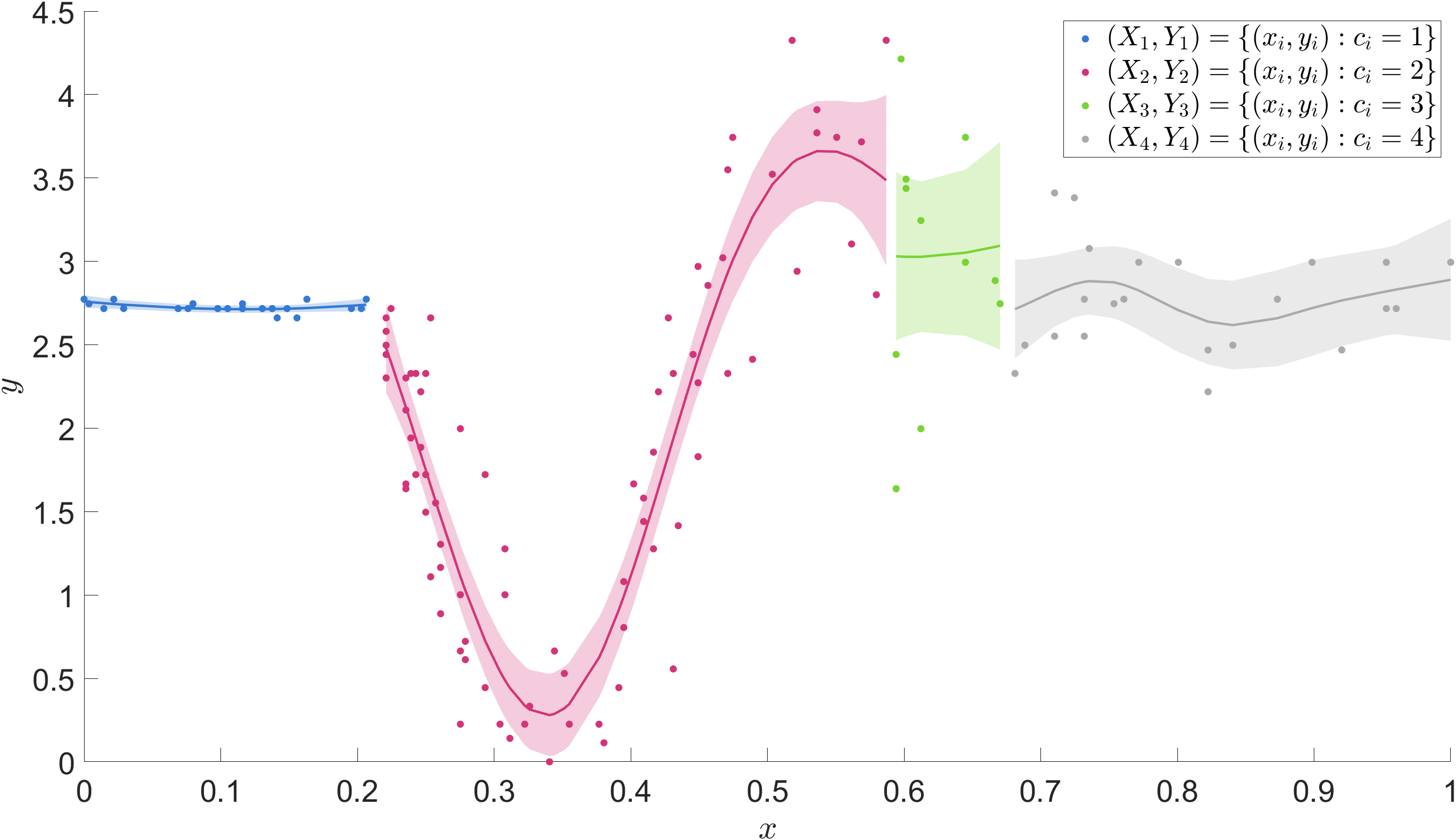
where $x_{i},x_{j}\in X_{k}$, $\sigma_{k,f}^{2}$ is the signal variance, and $l_{d}$ is the length scale along the $d$th dimension, with $\delta(x)$ denoting the Kronecker delta function and $\theta_{k}=(\sigma_{k,\varepsilon},\sigma_{k,f},l_{k,1},\ldots,l_{k,D})$. Furthermore, we use the notation $\Theta_{k}=(m_{k},\theta_{k})$ for the k$th$ GP parameters and $\Theta=(\Theta_{1},\ldots,\Theta_{K})$ for all the GP parameters. An example partition and and its corresponding GP fits are illustrated in Figure 1.

Figure 1: An example of partitioned data with four clusters. The clustered data points are shown in blue, red, green, and gray for each cluster with their respective GP mean and 95% pointwise credible intervals in the corresponding color.

2.2 Gating networks

We define the gating network through the kernels $\left\{\mathcal{K}_{1}(x_{i}\mid\psi_{1}),\dots,\mathcal{K}_{K}(x_{i}\mid\psi_{K})\right\}$; specifically,

$$p_{k}(x_{i})=\frac{\mathcal{K}_{k}(x_{i}\mid\psi_{k})}{\sum_{k^{\prime}=1}^{K}\mathcal{K}_{k^{\prime}}(x_{i}\mid\psi_{k^{\prime}})}.$$ (4)

To ensure the gating network ${\bf p}(x_{i})$ takes values in the $K-1$-dimensional simplex, we assume $0<\mathcal{K}_{k}(x\mid\psi)<\infty$ for all $x\in\mathbb{R}^{D}$. Examples of kernels used in literature include the multinomial logistic model with $\mathcal{K}_{k}(x\mid\psi_{k})=\exp(\psi_{k}^{T}x)$ (Li et al., 2011) and the factorized kernel $\mathcal{K}_{k}(x\mid\psi_{k})=v_{k}\prod_{d=1}^{D}\mathcal{K}_{k,d}(x_{d}\mid\psi_{k,d})$ (Antoniano-Villalobos et al., 2014). In the latter, mixed types of inputs are allowed by specifying each $\mathcal{K}_{k,d}(x_{d}\mid\psi_{k,d})$ to correspond to the kernel of standard distributions, depending on the nature of the $d$th input. We emphasize that this does not correspond to any model assumptions on the input, which in fact may be fixed.

In the following, we use weighted $D$-dimensional normal distributions for the kernels, individually denoted by $\mathcal{K}_{k}$:

$$\mathcal{K}_{k}(x_{i}\mid\psi_{k}):=\mathcal{K}_{k}(x_{i}\mid v_{k},\mu_{k},\Sigma_{k})=v_{k}\mathcal{N}(x_{i},\mid\mu_{k},\Sigma_{k}),$$ (5)

where $v_{k}$ denotes the weight of the component with $\mu_{k}\in\mathbb{R}^{D}$ and $\Sigma_{k}\in\mathbb{R}^{D\times D}$ being the mean and a diagonal covariance matrix, respectively. As such, we define $\psi_{k}:=(v_{k},\mu_{k},\Sigma_{k})^{T}=(v_{k},\mu_{k,1},\ldots,\mu_{k,D},\sigma^{2}_{k,1},\ldots,\sigma^{2}_{k,D})^{T}$ where $(\sigma^{2}_{k,1},\dots,\sigma^{2}_{k,D})$ are the diagonal elements of the $k$th covariance matrix. Hard cluster assignments using the above kernel result in quadratic boundaries. More flexible kernel specifications could be used for nonlinear boundaries such as mixtures of normals or the feature space method, where partitioning is done in a higher dimensional space, producing non-linear partitions in the original input space (Filippone et al., 2008). More generally, alternative specifications of the kernel may be employed.

For example, Zhang and Williamson (2019) also construct the gating network through normalized kernels and consider full covariance matrices $\Sigma_{k}$, employing the normal-inverse Wishart distribution as a prior for the means and covariances of the gating network. Instead the factorized form of the kernel based on a diagonal covariance matrix in Eq. (5) results in reduced computational complexity relative to the dimension $D$ of the inputs, from $\mathcal{O}(D^{3})$ in the case of the full covariance matrix to $\mathcal{O}(D)$ in the factorized form. Furthermore, the factorized form allows for straightforward extensions to include multiple input types, as in Antoniano-Villalobos et al. (2014). Lastly, the inverse-Wishart prior can suffer from poor parametrization (Consonni and Veronese, 2001), with only a single parameter to control variability. We instead follow Gelman (2006) in using independent half-normal distributions for the variance parameters. Additionally, we use a normal distribution for the mean $\mu_{k}$.

For the weights, we employ a Dirichlet prior:

$$(v_{1},\dots,v_{K})\sim\text{Dir}(\alpha/K,\dots,\alpha/K),$$ (6)

where $\alpha$ is the Dirichlet concentration parameter. The concentration parameter $\alpha$ can be used to enforce sparsity (Rousseau and Mengersen, 2011), as in sparse hierarchical MoEs. This helps to avoid overfitting, which is has been noted to be prevalent in dense mixtures (Titsias and Likas, 2002; Mossavat and Amft, 2011; Iikubo et al., 2018; İrsoy and Alpaydın, 2021). Smaller concentration parameter values promote sparsity, and in the extreme case when $\alpha\rightarrow 0$, prior mass is concentrated on the vertices of the simplex and all weight is placed on a single component. Thus, $K$ can be considered an upper bound on the number of components, and through appropriate selection of $\alpha$, the sparsity-promoting prior allows the data to determine the number of components required. In standard mixtures, Rousseau and Mengersen (2011) show that asymptotically the extra components will be emptied, provided that $\alpha/K<\varrho/2$, where $\varrho$ is the number of parameters in a single mixture component. Alternatively, the Jeffreys prior for the multinomial distribution, with $\alpha=K/2$ in our case, can be used as a simple non-informative choice (Grazian and Robert, 2018). The Dirichlet-distributed weights can also be constructed through independent Gamma random variables, that is $\nu_{1},\ldots,\nu_{K}$ are independent with $\nu_{k}\sim\text{Gamma}(\alpha/K,1)$ and defining each $v_{k}=\nu_{k}/\sum_{k^{\prime}=1}^{K}\nu_{k^{\prime}}$. Notice that the normalization term $\sum_{k=1}^{K}\nu_{k}$ cancels out in our definition of the gating network, so we can rewrite Eq. (5) as:

$$\mathcal{K}_{k}(x_{i}\mid\psi_{k}):=\mathcal{K}_{k}(x_{i}\mid v_{k},\mu_{k},\Sigma_{k})=\nu_{k}\mathcal{N}(x_{i},\mid\mu_{k},\Sigma_{k}).$$ (7)

2.3 Mixture of GP experts

Figure 2: Plate diagram showing relations between the data and model parameters for MoE.

This results in our statistical model being

$$\begin{split}Y_{k}\mid\left(X_{k},m_{k},\theta_{k}\right)&\sim\text{GP}\left(m_{k},\Sigma(X_{k},X_{k};\theta_{k})\right),\\ c_{i}\mid x_{i},\Psi&\sim\text{Categorical}({\mathbf{p}(x_{i})}),\\ \psi_{k}&\sim\pi_{0}(\psi_{k}),\\ \Theta_{k}&\sim\pi_{0}(\Theta_{k}),\end{split}$$ (8)

where $\pi_{0}(\Theta_{k})$ denotes the prior distribution for the GP parameters, which assumes independence across $k=1,\ldots,K$, and

$$p_{k}(x_{i})=\frac{\nu_{k}\mathcal{N}(x_{i},\mid\mu_{k},\Sigma_{k})}{\sum_{k^{\prime}=1}^{K}\nu_{k^{\prime}}\mathcal{N}(x_{i},\mid\mu_{k^{\prime}},\Sigma_{k^{\prime}})},$$ (9)

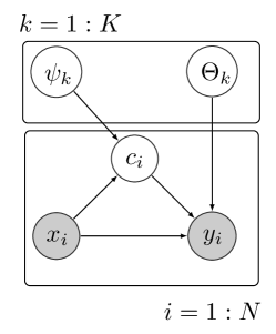
with $\nu_{k}\sim\text{Gamma}(\alpha/K,1)$ and $\mu_{k,d}$ and $\sigma^{2}_{k,d}$ assigned independent normal and half-normal priors, respectively. A plate diagram of the model is provided in Figure 2.

3 Importance sampling

Zhang and Williamson (2019) propose an embarrassingly parallel algorithm based on importance sampling (IS) to estimate the posterior distribution of $C$ and $\Psi$, using a MAP approximation for the GP parameters $\Theta$ as well as the predictive distribution of the data in parallel. For this, an importance distribution $q(C,\Psi\mid X)$ is constructed which is easy to sample from. The importance distribution is chosen to be the prior distribution such that $q(C,\Psi\mid X)=\pi(C,\Psi\mid X)$. Thus,

$$\begin{split}q(C,\Psi\mid X)&=p(C\mid X,\Psi)\pi(\Psi)=\prod_{i=1}^{N}p(c_{i}|x_{i},\Psi)\prod_{k=1}^{K}\pi_{0}(\psi_{k})\\ &=\prod_{k=1}^{K}\prod_{i:c_{i}=k}\frac{v_{k}N(x_{i}\mid\mu_{k},\Sigma_{k})}{\sum_{k^{\prime}=1}^{K}v_{k^{\prime}}N(x_{i}\mid\mu_{k^{\prime}},\Sigma_{k^{\prime}})}\pi_{0}(\psi_{k}).\end{split}$$ (10)

Using the above, $J$ particles are sampled in parallel from $q(C,\Psi\mid X)$ and the weight $\omega_{j}$ for the $j$th particle $(C_{j},\Psi_{j})$ in the IS estimation is given as

$$\begin{split}\omega_{j}&\propto\frac{\pi(C_{j},\Psi_{j}\mid X,Y)}{q(C_{j},\Psi_{j}\mid X)}\propto\frac{p(Y\mid X,C_{j},\Psi_{j})\pi(C_{j},\Psi_{j}\mid X)}{\pi(C_{j},\Psi_{j}\mid X)}\\ &=p(Y\mid X,C_{j},\Psi_{j})\approx\prod_{k=1}^{K}\mathcal{N}\left(Y_{k,j}\mid\widehat{m}_{k,j},\Sigma(X_{k},X_{k};\widehat{\theta}_{k,j})\right),\end{split}$$ (11)

where $\widehat{m}_{k,j}$ and $\widehat{\theta}_{k,j}$ are MAP estimates. For a new input $x^{*}$, the predictive mean and density of the output are computed by averaging according to the respective particle weights and gating network probabilities at the new location $x^{*}$:

$$\mathbb{E}[y^{*}\mid x^{*},X,Y] =\sum\limits_{j=1}^{J}\omega_{j}\sum\limits_{k=1}^{K}m^{*}_{k,j}\,p_{k}(x^{*}\mid\Psi_{j}),$$

$$\pi(y^{*}\mid x^{*},X,Y) =\sum\limits_{j=1}^{J}\omega_{j}\sum\limits_{k=1}^{K}\mathcal{N}(y^{*}\mid m^{*}_{k,j},\Sigma^{*}_{k,j})\,p_{k}(x^{*}\mid\Psi_{j}),$$

where $m^{*}_{k,j}$ and $\Sigma^{*}_{k,j}$ are the predictive mean and covariance of the associated $K$ GPs for each of the $J$ particles. For more details on the importance sampling approach, see Zhang and Williamson (2019).

As mentioned in the Introduction, the number of particles required for importance sampling is exponential in the KL divergence of the posterior from the proposal distribution (Chatterjee and Diaconis, 2018), that is $J\propto\exp[{D_{\text{KL}}(\pi(C,\Psi\mid X,Y)\,\|\,q(C,\Psi\mid X))}]$. As an extreme example, consider a uniform proposal distribution for $C$, with $q(C\mid X,\Psi)=1/K^{N}$, obtained in the limiting case when $\alpha\rightarrow\infty$ and $\sigma^{2}_{k,d}\rightarrow\infty$. On the other hand, suppose the posterior on $C$ is very concentrated on a single partition $C^{*}$; due to invariance with respect to a relabelling of the components, the posterior in this case is uniform over the set $\mathcal{C}$ of $C$ that are equivalent to $C^{*}$ up to relabelling of the components. Thus, $\pi(C\mid X,Y)=\sum_{C\in\mathcal{C}}1/|\mathcal{C}|\delta_{C}$, where the size of $\mathcal{C}$ is $|\mathcal{C}|={K\choose t}t!$, with $t$ denoting the number of clusters in $C^{*}$. Here, the KL divergence is:

$${D_{\text{KL}}(\pi(C,\Psi\mid X,Y)\,\|\,q(C,\Psi\mid X))}=\sum_{C\in\mathcal{C}}1/|\mathcal{C}|\log\left(\frac{K^{N}}{|\mathcal{C}|}\right)=\log\left(\frac{K^{N}}{{K\choose t}t!}\right),$$

and the number of particles required is $J\propto K^{N}/({K\choose t}t!)$. Even for a very small sample size, e.g. $N=10$, $K=5$, and $t=2$, this requires $J\propto 488,281$, and when $N=20$, this increases to $J\propto 4,768,371,582,031$.

While this is a purposefully constructed edge case, some insight on behaviour for stationary data in comparison to data that present departures, such non-stationary, discontinuity, or heteroskedasticity, can be postulated. Stationary data can be modelled well over a large class of partitions, as all data can be effectively be modelled via a single GP model and partitioning into any reasonable number of subgroups will not degrade the fit too much. Therefore, sampling of the partitions can be done effectively using strategies such importance sampling as the “distance” between the proposal and posterior are smaller in comparison to non-stationary and discontinuous cases. Instead, the partitions play a more important part in modelling non-stationary and discontinuous data; the posteriors are clearly concentrated on a smaller number of partitions thus requiring more samples to have a suitable approximation.

This motivates us to use SMC methods, and specifically SMC², to improve our estimation of the posterior or retain the same level of quality with the same number of or fewer particles.

4 SMC²

Sequential Monte Carlo (SMC) methods, also known as particle filtering and smoothing, are a standard tool in statistical signal processing (Särkkä, 2013) and provide a robust method for sampling posterior distributions (Chopin, 2002; Del Moral et al., 2006). As SMC methods employ a collection of weighted particles, their application is a natural extension to the methodology presented in Zhang and Williamson (2019).

We use sequential likelihood tempering to estimate the gating network parameters $\Psi$ and the allocation variables $C$, while fitting $K$ independent Gaussian processes to the partitioned data. This is done to improve the importance distribution, especially for complex target distributions. Using the discriminative MoE model in Section 2.3, the target posterior distribution for $C$, $\Psi$, and $\Theta$ is

$$\pi(C,\Psi,\Theta\mid X,Y)\propto p(Y\mid X,C,\Theta)p(C\mid X,\Psi)\pi_{0}(\Psi)\pi_{0}(\Theta),$$ (12)

which can be marginalized with respect to the GP parameters $\Theta$ to yield

$$\pi(C,\Psi\mid X,Y)\propto p(Y\mid X,C)p(C\mid X,\Psi)\pi_{0}(\Psi).$$ (13)

In this case, the likelihood $p(Y\mid X,C)$ is given as

$$\begin{split}p(Y\mid X,C)&=\int p(Y\mid X,C,\Theta)\pi_{0}(\Theta)\,\text{d}\Theta=\prod\limits_{k=1}^{K}\int p\left(Y_{k}\mid X_{k},\Theta_{k}\right)\pi_{0}(\Theta_{k})\,\text{d}\Theta_{k},\end{split}$$ (14)

with log-likelihood of the individual GPs being

$$\begin{split}\log p(Y_{k}\mid X_{k},\Theta_{k})=&-\frac{1}{2}(Y_{k}-m_{k})^{T}\Sigma(X_{k},X_{k};\theta_{k})^{-1}(Y_{k}-m_{k})\\ &-\frac{1}{2}\log\left|\Sigma(X_{k},X_{k};\theta_{k})\right|-\frac{N_{k}}{2}\log 2\pi,\end{split}$$ (15)

where $\left|\Sigma(X_{k},X_{k};\theta_{k})\right|$ is the determinant of the covariance matrix and $N_{k}$ is the number of data points in the $k$th group. The tempered conditional posterior distribution for the parameters $C$ and $\Psi$, can be then given as

$$\pi_{t}(C,\Psi\mid X,Y)\propto p_{t}(Y\mid X,C)p(C\mid X,\Psi)\pi_{0}(\Psi),$$ (16)

with

$$p_{t}(Y\mid X,C):=\int_{\Theta}p(Y\mid X,C,\Theta)^{\kappa^{(t)}}\pi_{0}(\Theta)\,\text{d}\Theta=\prod\limits_{k=1}^{K}\int p\left(Y_{k}\mid X_{k},\Theta_{k}\right)^{\kappa^{(t)}}\pi_{0}(\Theta_{k})\,\text{d}\Theta_{k},$$ (17)

and where $t$ stands for the “time” step of SMC² and $\kappa^{(t)}$ is a strictly increasing sequence of parameters, $0=\kappa(0)<\dots<\kappa(t-1)<\kappa(t)<\dots<\kappa(T)=1$, controlling the degree of tempering.

We unbiasedly estimate the tempered marginal likelihood $p_{t}(Y\mid X,C)$ by an ensemble $\{\Theta_{j,m}^{(t)}\}_{m=1}^{M}$ for each particle $(C,\Psi)_{j}^{(t)}$, as follows. We have the tempered unnormalized posterior

$$\pi_{t}(Y,C,\Psi,\Theta)=\prod_{s=1}^{t}p(Y\mid X,C,\Theta)^{\kappa^{(s)}-\kappa^{(s-1)}}\pi(C,\Psi,\Theta\mid X).$$ (18)

Now, for any given $(C,\Psi)$, we can construct a non-negative and unbiased estimator of the joint $\pi_{t}(Y,C,\Psi)$ as

$$\hat{\pi}_{t}(Y,C,\Psi)=\widehat{Z}^{M}_{t}(Y\mid X,C)\pi(C,\Psi\mid X)\,,$$ (19)

where

$$\widehat{Z}^{M}_{t}(Y\mid X,C):=\prod_{s=1}^{t}\frac{1}{M}\sum_{m=1}^{M}p(Y\mid X,C,\Theta^{(s-1)}_{m})^{\kappa^{(s)}-\kappa^{(s-1)}}\,,$$ (20)

is a non-negative and unbiased estimator of $p_{t}(Y\mid X,C)$ in Eq. (17) with $\Theta^{(s)}_{m}$ being the output from an SMC with fixed $C$. In other words, $\Theta^{(0)}_{m}$ are i.i.d from the prior $\Theta^{(0)}_{m}\sim\pi_{0}(\Theta)$, and for $t=1,\dots,T$, $\Theta^{(t)}_{m}\sim\mathcal{M}_{t}(\widehat{\,\Theta}^{(t)}_{m},\,\cdot)$, where $\widehat{\Theta}^{(t)}_{m}=\Theta_{I_{m}^{(t)}}^{(t)}$ and $I_{m}^{(t)}\sim\text{Categorical}({\bf\omega}^{(t)})$ for $m=1,\dots,M$, with ${\bf\omega}^{(t)}=(\omega^{(t)}_{1},\dots,\omega^{(t)}_{M})$ and $\omega^{(t)}_{m}\propto p(Y\mid X,C,\Theta^{(t-1)}_{m})^{\kappa^{(t)}-\kappa^{(t-1)}}$. Here $\mathcal{M}_{t}$ is an MCMC kernel which keeps

$$p_{t}(\Theta\mid C,X,Y)\propto\pi_{t}(Y,C,\Psi,\Theta)$$ (21)

invariant. Let $A^{(t)}$ denote $I_{1:M}^{(1:t)}$ and all the auxiliary variables of the SMC sampler for $\Theta$. The distribution

$$\pi_{t}(C,\Psi,\Theta_{1:M}^{(0:t)},A^{(t)}\mid X,Y)\propto\widehat{Z}^{M}_{t}(Y\mid X,C)\pi(C,\Psi\mid X){\Upsilon}(\Theta_{1:M}^{(0:t)},A^{(t)}\mid C,X,Y),$$ (22)

where ${\Upsilon}(\Theta_{1:M}^{(0:t)},A^{(t)}\mid C,X,Y)$ is the distribution of the SMC sampler given $C$ (up to time $t$), is such that for any $m=1,\dots,M$ and any $t=0,\dots,T$,

$$\int\varphi(C,\Psi,\Theta)\,d\pi_{t}(C,\Psi,\Theta\mid X,Y)=\int\varphi(C,\Psi,\Theta^{(t)}_{m})\,d\pi_{t}(C,\Psi,\Theta_{1:M}^{(0:t)},A^{(t)}\mid X,Y).$$ (23)

In other words, it has the target of interest as its marginal. We note that the SMC sampler ${\Upsilon}$ is independent of $\Psi$, hence its omission. Targeting $\pi_{t}(C,\Psi,\Theta_{1:M}^{(0:t)},A^{(t)},\mid X,Y)$ using MCMC is called particle MCMC (PMCMC) and is a particular instance of the pseudo-marginal method (Andrieu and Roberts, 2009). When the MCMC method used is Metropolis-Hastings, it is called particle marginal Metropolis-Hastings (PMMH) (Andrieu et al., 2010). In particular, the proposal consists of sampling $(C,\Psi)^{*}\sim\mathcal{Q}((C,\Psi)_{m},\cdot)$ and then $(\Theta_{1:M}^{(0:t)})^{*}\sim{\Upsilon}(\Theta_{1:M}^{(0:t)},A^{(t)}\mid C^{*},\Psi^{*})$. The proposal $(C,\Psi,\Theta_{1:M}^{(0:t)})^{*}$ is then accepted with probability

$$\frac{\widehat{Z}^{M}_{t}(Y\mid X,C^{*})\pi((C,\Psi)^{*}\mid X)\mathcal{Q}((C,\Psi)^{*},(C,\Psi)_{m})}{\widehat{Z}^{M}_{t}(Y\mid X,C_{m})\pi((C,\Psi)_{n}\mid X)\mathcal{Q}((C,\Psi)_{m},(C,\Psi)^{*})}.$$ (24)

We denote the resulting MCMC kernel by $\mathcal{H}_{t}$ and note that by design $\pi_{t}\mathcal{H}_{t}=\pi_{t}$. We target $\pi_{t}(C^{(t)},\Psi^{(t)},\Theta_{1:M}^{(0:t)},A^{(t)}\mid X,Y)$ for $t=1,\dots,T$ using an SMC sampler (Del Moral et al., 2006), where the MCMC mutation at time $t$ is given by the PMMH kernel $\mathcal{H}_{t}$ (indices $t$ are introduced on the variables for convenience and to avoid confusion). This method is called SMC² owing to the nested SMCs (Chopin et al., 2013).

In particular, we approximate (22) using the particles $\{C_{j}^{(t)},\Psi_{j}^{(t)},(\Theta_{1:M}^{(0:t)})_{j}\}_{j=1}^{J}$ with weights $\{w_{j}^{(t)}\}_{j=1}^{J}$. Note that we do not need the auxiliary variables $A^{(t)}_{j}$, as they will always be integrated out. In fact, for estimates we also only need one $\Theta_{j,m}^{(t)}$ for each $j$, sampled uniformly from $\left(\Theta_{j,m}^{(t)},\dots\Theta_{j,M}^{(t)}\right)$, however in principle one can average over the ensemble, which is a Rao-Blackwellisation of the former. Furthermore, if we do not need to estimate functions of $\Theta$, then we only need the normalizing constant estimates $\widehat{Z}^{M}_{t}(Y\mid X,C_{j}^{(t)})$ along with the $(C,\Psi)_{j}^{(t)}$ particles. For $J$ particles, estimating the tempered posterior in Eq. (16) using the model on the extended state space given in Eq. (22), the particle weights are recursively related according to

$$w_{j}^{(t)}\propto\frac{\widehat{Z}^{M}_{t}(Y\mid X,C_{j})}{\widehat{Z}^{M}_{t-1}(Y\mid X,C_{j})}w_{j}^{(t-1)}=\sum\limits_{m=1}^{M}p_{t}(Y\mid X,C_{j},\Theta_{m}^{(t-1)})^{\kappa^{(t)}-\kappa^{(t-1)}}w_{j}^{(t-1)},$$ (25)

where the initial particle weights are set as $w_{j}^{(0)}=\frac{1}{J}$. However, the recursive update to the particle weights degrades the sample distribution. This degradation can be quantified using the effective sample size (ESS):

$$J_{\text{ESS}}^{(t)}=\frac{1}{\sum\limits_{j=1}^{J}\left(w_{j}^{(t)}\right)^{2}}.$$ (26)

We determine $\kappa^{(t)}$ adaptively so that the relative reduction in the ESS is approximately a predefined learning rate, $\eta$. In particular, we resample the particles after each iteration $t$ of the algorithm. This introduces duplicates of the particles into the sample. The MCMC mutation with $\mathcal{H}_{t}$ counteracts this.

In particular, we propose new $\Psi^{*}_{1:J}$ particles by separately proposing the gating network means and standard deviations from the weights. We construct the random walk proposal for the means and standard deviations as

$$(\mu_{1:K},\Sigma_{1:K})^{*}_{j}=(\mu_{1:K},\Sigma_{1:K})_{j}+\xi_{\mu,\Sigma,j}$$ (27)

where $\xi_{\mu,\Sigma,j}\sim\mathcal{N}(0,\Sigma_{\mu,\Sigma})$ with $\Sigma_{\mu,\Sigma}\in\mathbb{R}^{N_{\mu,\Sigma}\times N_{\mu,\Sigma}}$ and $N_{\mu,\Sigma}=2DK$, being the weighted empirical covariance matrix of the $J$ particles, $(\mu_{1:K},\Sigma_{1:K})_{1:J}$. We enforce positivity of the variance parameters by rejecting negative proposals due to our choice of prior distributions. The gating network weights, as in Lukens et al. (2020), are proposed as

$$\log\nu_{1:K,j}^{*}=\log\nu_{1:K,j}+\xi_{\nu,j}$$ (28)

where $\xi_{\nu,j}\sim\mathcal{N}(0,\Sigma_{\nu})$ with $\Sigma_{\nu}\in\mathbb{R}^{N_{\nu}\times N_{v}}$ and $N_{v}=K$, being the weighted empirical covariance matrix of the $J$ particles of the weights.

The proposal for the partition $C^{*}$ given the proposed gating network parameters $\Psi^{*}$ follows the prior, that is $c^{*}_{i}\sim\text{Categorical}(\mathbf{p}(x_{i}\mid\Psi^{*}))$ independently for $i=1,\ldots,n$. This leads to convenient cancellations in the acceptance probability. In cases when the clusters are not well separated by the inputs, we may need better proposals for the partitions. Possible alternatives are single-site Gibbs sampling (Rasmussen and Ghahramani, 2002) or split-merge moves which update multiple allocation variables simultaneously, first appearing in Jain and Neal (2004) and more recently in Bouchard-Côté et al. (2017).

For the inner SMC, we use similar MCMC updates as for the outer SMC. The proposals are constructed independently for each of the $K$ experts. We propose new $\Theta_{k,j,m}^{*}$ particles again with a random walk proposal given as

$$\Theta_{k,j,m}^{*}=\Theta_{k,j,m}+\xi_{\Theta_{k,j},m}$$ (29)

where $\xi_{\Theta_{k,j},m}\sim\mathcal{N}(0,\Sigma_{{\Theta_{k,j}}})$ with $\Sigma_{{\Theta_{k,j}}}\in\mathbb{R}^{N_{\theta}\times N_{\theta}}$ and $N_{\theta}=D+3$, being the weighted empirical covariance matrix of the $M$ inner particles, $\left(\Theta_{k,j,1},\dots,\Theta_{k,j,M}\right)$, corresponding to the GP parameters of the $k$th expert. Positivity of the variance parameters is again enforced via our choice of prior distributions.

We use a criteria to automatically adapt the number of MCMC steps taken to mutate the particles suggested by Chopin et al. (2013). In particular, we perform MCMC steps until a relative decrease in a distance metric is below a given threshold $\delta$

$$\dfrac{\left|d^{(n)}-d^{(n-1)}\right|}{d^{(n-1)}}<\delta,$$ (30)

where

$$d^{(n)}=\frac{1}{N_{\rho}}\sum\limits_{i=1}^{N_{\rho}}\left\|\rho_{i}^{(n)}-\rho_{i}^{(0)}\right\|_{2},$$ (31)

where $\|\cdot\|_{2}$ denotes Euclidean norm. Here, $\rho$ denotes the set of parameters being updated in the MCMC, i.e. $\rho=(\Psi_{j},C_{j})$ in the outer SMC and $\rho=(\Theta_{k,j,m})$ for the inner SMC. For the $n$th MCMC step, $\rho_{i}^{(n)}$ denotes the $i$th of $N_{\rho}$ particles for the inner SMCs, while for the outer SMC, $\rho_{i}^{(n)}$ denotes the $i$th of $N_{\rho}$ unbiased estimates of the likelihood in Eq. (19). For the outer SMC, we monitor the change in the likelihood in Eq. (19) as it is invariant to label-switching.

Before ending this section, it is relevant to reflect on the complexity of this method. Just as with naive importance sampling, the cost is ultimately dominated by the Gaussian process likelihoods with complexities proportional to $\mathcal{O}(KN^{3}/K^{3})$, assuming $N/K$ data points for each of the $K$ experts, which can be distributed across the $K$ experts. The likelihood needs to estimated for each of $M$ inner and $J$ outer $\Theta_{j,m}$ particles at each time step $t=0,\dots,T$. For the mutation PMCMC step, this must be done $t$ times at step $t$, that is when the clustering $C$ changes we must initialize the particles $\Theta_{j,m}\sim\pi_{0}(\Theta)$ from the prior and rerun the inner SMC sampler. Therefore, the total number of likelihood estimations is $MJ\sum_{t=0}^{T}t=\mathcal{O}(T^{2}MJ)$, and the total cost is $\mathcal{O}(T^{2}MJN^{3}/K^{2})$. This seems expensive, particularly if one makes the natural choice $T,M,J\propto N$, see for example Chopin et al. (2013); Beskos et al. (2014); Chopin and Papaspiliopoulos (2020), but the point is that, in comparison to naive importance sampling, $N^{4}$ is much less than the number samples required in importance sampling, e.g. $N^{4}\ll K^{N}$ in the example of Section 3. Moreover, many evaluations can be performed in parallel.

5 Predictive distribution

Algorithm 1 SMC² sampled Mixture of Gaussian Process Experts.

Initialize:

      Set $t=0$ and $\kappa^{(t)}=0$.

      Draw $U^{(0)}_{j}\sim p(C,\Psi,\Theta_{1},\dots\Theta_{M}\mid X)$,

      Set $\widehat{Z}^{M}_{0}(C_{j})=1$.

      Set initial weights $\mathbf{w}^{(0)}=(w_{1}^{(0)},\dots,w_{J}^{(0)})$, where $w_{j}^{(0)}=\frac{1}{J}$.

Estimation of $\pi(C,\Psi,\Theta\mid X,Y)$:

while $\kappa_{t}<1$ do

     $t=t+1$.

     Determine $\kappa^{(t)}$.

     Resample $U^{(t)}_{j}$ given particles weights ${\bf w}^{(t)}$, where $w_{j}^{(t)}$ follow Eq. (25).

     Set $w_{j}^{(t)}=\frac{1}{J}$.

     Run one step of the inner SMC sampler for $U^{(t-1)}_{j}$ to obtain $\widehat{U}^{(t)}_{j}$.

     Update $\widehat{Z}^{M}_{t}(C_{j})$ according to Eq. (20).

     Draw $\widetilde{U}^{(t)}_{j}\sim\mathcal{K}_{t}(\widehat{U}^{(t)}_{j},\,\cdot)$, where $\mathcal{K}_{t}$ is a PMCMC kernel targeting $\pi_{t}$ in Eq. (22).

     Set $U^{(t)}_{j}=\widetilde{U}^{(t)}_{j}$.

end while

Prediction:

      Compute the predictive distributions according to Eq. (36).

We construct the predictive distribution by computing the individual GP predictive distributions for each expert given the partition $C_{j}$ and GP parameters $\Theta_{j,m}$, for every particle. These are then weighted by the particle weights and the gating network with parameters $\Psi_{j}$. Specifically, for each of the $K$ GPs, the predictive mean and variance for a given input $x^{*}\in\mathbb{R}^{D}$ is given by

$$\mathbb{E}_{y^{*}_{k,j,m}}:=\mathbb{E}\left[y^{*}\mid x^{*},X,Y,C_{j},\Psi_{j},m_{k,j,m},\theta_{k,j,m}\right]=\Sigma_{*}\Sigma_{X}^{-1}(Y_{k,j}-m_{k,j,m})+m_{k,j,m},$$ (32)

and

$$\text{Var}_{y^{*}_{k,j,m}}:=\text{Var}\left[y^{*}\mid x^{*},X,Y,C_{j},\Psi_{j},m_{k,j,m},\theta_{k,j,m}\right]=\Sigma_{**}-\Sigma_{*}\Sigma_{X}^{-1}\Sigma_{*}^{T},$$ (33)

where $\Sigma_{**}=\Sigma(x^{*},{x^{*}};\theta_{k,j,m})$, $\Sigma_{*}=\Sigma(x^{*},X_{k,j};\theta_{k,j,m})$, and $\Sigma_{X}=\Sigma(X_{k,j},X_{k,j};\theta_{k,j,m})$ are used for brevity. The individual normal marginal predictive distributions are combined into a mixture distribution:

$$\pi(y^{*}\mid c^{*}=k,x^{*},X,Y,C_{j},\Psi_{j})=\sum\limits_{m=1}^{M}\omega_{m}\mathcal{N}(y^{*}\mid\mathbb{E}_{y^{*}_{k,j,m}},\text{Var}_{y^{*}_{k,j,m}}),$$ (34)

which, in practice, would be evaluated over a grid of $y^{*}$ values for each $x^{*}$ value where prediction is desired. These mixture distributions are further compounded across the $K$ experts according to

$$\pi(y^{*}\mid x^{*},X,Y,C_{j},\Psi_{j})=\sum\limits_{k=1}^{K}\pi(y^{*}_{j}\mid c^{*}=k,x^{*},X,Y,C_{j},\Psi_{j})p_{k}(x^{*}\mid\Psi_{j}),$$ (35)

where the distributions are weighted according to the gating network defined in Eq. (4). Lastly, the distributions obtained for each $(C_{j},\Psi_{j})$ particle are added together according to their particle weights as

$$\pi(y^{*}\mid x^{*},X,Y)=\sum\limits_{j=1}^{J}w_{j}\pi(y^{*}\mid x^{*},X,Y,C_{j},\Psi_{j}).$$ (36)

Similarly, the predictive mean is computed as

$$\mathbb{E}[y^{*}\mid x^{*},X,Y]=\sum\limits_{j=1}^{J}w_{j}\sum\limits_{k=1}^{K}p_{k}(x^{*}\mid\Psi_{j})\sum\limits_{m=1}^{M}\omega_{m}\,\mathbb{E}_{y^{*}_{k,j,m}}.$$ (37)

Note that by resampling at each iteration $t$, the weights are $w_{j}=\frac{1}{J}$ and $\omega_{i}=\frac{1}{M}$. Pseudo-code for the method is shown in Algorithm 1.

6 Numerical examples

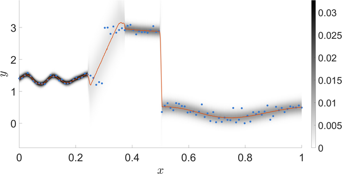
We demonstrate the method using multiple simulated and real-life one-dimensional data sets along with a multi-dimensional data set. The simulated one-dimensional sets of data consist of 1) a continuous function with homoskedastic noise and 2) a discontinuous function with heteroskedastic noise. The first data set is generated using

$$y_{k}=\sin(\pi x_{k})\cos((\pi x_{k})^{3})+\varepsilon(x_{k})$$ (38)

where $\varepsilon(x_{k})\sim\mathcal{N}(0,0.15^{2})$ meaning that the measurement noise is homoskedastic. In contrast, the second data set is generated by

$$y_{k}=\begin{cases}\sin(60x_{k})-2+\varepsilon_{1}(x_{k}),&x_{k}\leq 0.3\\ 10+\varepsilon_{2}(x_{k}),&0.3<x_{k}\leq 0.5\\ \sin(4\pi x_{k})-10+\varepsilon_{3}(x_{k})&0.5<x_{k}\leq 1\end{cases}$$ (39)

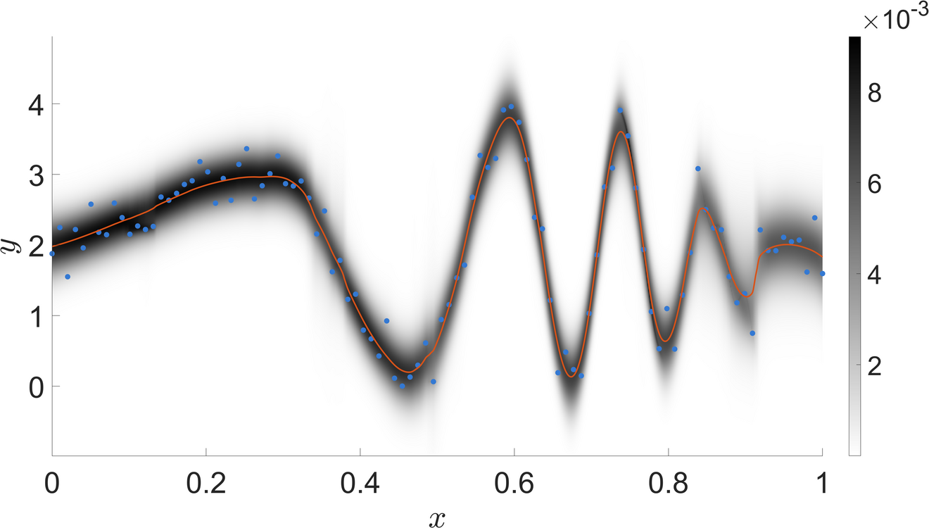
where $\varepsilon_{1}(x_{k})\sim\mathcal{N}(0,0.05^{2})$, $\varepsilon_{2}(x_{k})\sim\mathcal{N}(0,0.025^{2})$, and $\varepsilon_{3}(x_{k})\sim\mathcal{N}(0,0.10^{2})$ are used to generate heteroskedastic measurement errors. We also consider the motorcycle data set studied in Silverman (1985), which shows obvious heteroskedastic noise and non-stationarity, with areas exhibiting different behaviours. The data measures head acceleration in a simulated motorcycle accident for testing helmets; the measurements are practically constant initially, with a low noise level, which abruptly turns oscillating with high noise and gradually decaying to a possibly constant state while still having clearly higher measurement noise in comparison to the initial constant state. Lastly, we also study the multi-dimensional Langley glide-back booster simulation data set. The Langley glide-back booster is a rocket booster designed by NASA to allow the booster to glide down from the atmosphere instead of requiring crashing it into the ocean. A more detailed description of the booster and the related data set is provided in Gramacy and Lee (2008). As in Gramacy and Lee (2008), we model the lift as the output variable and the input variables include the vehicle speed at atmospheric re-entry, angle of attack, and the sideslip angle which are referred to in the data set as Mach, $\alpha$, and $\beta$, respectively. The data set consists of $3167$ data points of which we use the subset of $N=1900$ data points.

Parameter	Prior distribution
$\mu_{k}$	$\mathcal{N}\left(\frac{k}{K+1},\left(0.25\times\frac{1}{K+1}\right)^{2}\right)$
$\sigma_{k}$	$\mathcal{N}_{\frac{1}{2}}\left(0,\left(0.25\times\frac{1}{K+1}\right)^{2}\right)$
$m_{k}$	$\mathcal{U}\left(0,\max Y\right)$
$\sigma_{k,\varepsilon}$	$\mathcal{N}_{\frac{1}{2}}\left(0,0.25^{2}\right)$
$\sigma_{k,f}$	$\mathcal{N}_{\frac{1}{2}}\left(0,0.25^{2}\right)$
$l_{k}$	$\mathcal{N}_{\frac{1}{2}}\left(0,0.125^{2}\right)$

Table 1: Prior distributions for $\Psi$ and $\Theta$ for the one-dimensional data sets. To encourage components that are well-separated along the input space, the prior means for the gating networks parameters $\mu_{k}$ are constructed using a linearly-spaced grid, with identical prior variances.

Parameter	Prior distribution
$\mu_{k,d}$	$\mathcal{N}\left(G_{k,d},\left(0.05\times\frac{1}{\sqrt[D]{K}+1}\right)^{2}\right)$
$\sigma_{k,d}$	$\mathcal{N}_{\frac{1}{2}}\left(0,\left(0.01\times\frac{1}{\sqrt[D]{K}+1}\right)^{2}\right)$
$m_{k}$	$\mathcal{U}\left(0,\max Y\right)$
$\sigma_{k,\varepsilon}$	$\mathcal{N}_{\frac{1}{2}}\left(0,0.25^{2}\right)$
$\sigma_{k,f}$	$\mathcal{N}_{\frac{1}{2}}\left(0,0.25^{2}\right)$
$l_{k,1}$	$\mathcal{N}_{\frac{1}{2}}\left(0,0.125^{2}\right)$

Table 2: Prior distributions for $\Psi$ and $\Theta$ for the NASA booster data set. To encourage components that are well-separated along the input space, the prior means for the gating networks parameters $\mu_{k}$ are constructed using a linearly-spaced grid, so that spacing along each dimension is $1/\sqrt[D]{K}$, with $G_{k}=(G_{k,1},\ldots,G_{k,D})$ denoting the $k$th grid point.

For all data sets, the inputs and outputs are normalized such that $X\in[0,1]^{D}$, $\min Y=0$, and $\text{Var}[Y]=1$. The prior distributions for the gating network parameters $\Psi$ and experts parameters $\Theta$ are summarized in Tables 1 and 2 for the one-dimensional and multi-dimensional data sets, respectively. Specifically, we use normal and half-normal priors for the gating network means and variances, respectively, along with a uniform prior for the GP constant mean functions and half-normal priors for variance and length scale parameters of the GPs. To encourage well-separated components along the input space, the prior means for the gating network parameters are constructed using a linearly-spaced grid along each dimension.

(a)

(b)

(c)

(d)

(e)

(f)

(g)

(h)

(i)

(j)

Figure 3: First synthetic data set: non-stationary function, homoskedastic noise. In a), the generated data points are shown (in blue) with a heat map of the underlying ground truth distribution in black and the true function as a solid red line. In b), c), and d) the predictive distribution for MoE with SMC² is shown for different values of the Dirichlet concentration parameter $\alpha=0.1,1,K/2$. In e), f), and g) the predictive distributions are shown for IS-MoE with the same Dirichlet concentration parameters. In the bottom row, h), i), and j) show the predictive distributions for a single GP, RBCM, and treedGP, respectively.

(a)

(b)

(c)

(d)

(e)

(f)

(g)

(h)

(i)

(j)

Figure 4: Second synthetic data set: discontinuous function, heteroskedastic noise. In a) the generated data points are shown (in blue) with a heat map of the underlying ground truth distribution in black and the true function as a solid red line. In b), c), and d) the predictive distribution for MoE with SMC² is shown for different values of the Dirichlet concentration parameter $\alpha=0.1,1,K/2$. In e), f), and g) the predictive distributions are shown for IS-MoE with same Dirichlet concentration parameters. In the bottom row, h), i), and j) show the predictive distributions given for a single GP, RBCM, and treedGP, respectively.

	$L^{1}$	$L^{2}$	$L^{1}$ median
SMC2-MoE, $\alpha=0.1$	375.731	0.860	135.978
SMC2-MoE, $\alpha=1$	402.887	0.881	139.738
SMC2-MoE, $\alpha=K/2$	403.566	0.893	138.866
IS-MoE, $\alpha=0.1$	588.068	1.042	154.580
IS-MoE, $\alpha=1$	599.560	1.073	159.100
IS-MoE, $\alpha=K/2$	602.536	1.075	159.797
GP	373.676	0.912	142.085
RBCM	424.606	1.063	148.719
TreedGP	363.797	0.855	134.044

Table 3: First synthetic data set: non-stationary function, homoskedastic noise. Column $L^{1}$ shows the $L^{1}$ vector norm of the difference between the estimated distributions and the ground truth distribution used to generate the data set for a given method. Column $L^{2}$ shows the $L^{2}$ vector norm of the difference between the aforementioned distributions and column $L^{1}$ median shows the $L^{1}$ vector norm of the distance between the posterior predictive median and the ground truth median.

	$L^{1}$	$L^{2}$	$L^{1}$ median
SMC2-MoE, $\alpha=0.1$	509.876	2.368	46.418
SMC2-MoE, $\alpha=1$	530.417	2.406	46.407
SMC2-MoE, $\alpha=K/2$	558.190	2.499	47.203
IS-MoE, $\alpha=0.1$	993.265	3.301	84.464
IS-MoE, $\alpha=1$	934.844	3.167	85.765
IS-MoE, $\alpha=K/2$	925.779	3.133	85.209
GP	1078.485	3.496	95.274
RBCM	1217.425	3.770	187.151
TreedGP	655.436	2.857	87.843

Table 4: Second synthetic data set: discontinuous function, heteroskedastic noise. Column $L^{1}$ shows the $L^{1}$ vector norm of the difference between the estimated distributions and the ground truth distribution used to generate the data set for a given method. Column $L^{2}$ shows the $L^{2}$ vector norm of the difference between the aforementioned distributions and column $L^{1}$ median shows the $L^{1}$ vector norm of the distance between the posterior predictive median and the ground truth median.

Figure 5: First synthetic data set: non-stationary function, homoskedastic noise. On the left, the predictive distributions and median for SMC²-MoE are shown in black and red, along with the data points in blue, for different values of the Dirichlet concentration parameter $\alpha$. In the middle column, the posterior distribution for the number of non-empty experts is shown. The last column shows the posterior similarity matrices summarizing the posterior over partitions. Values of $\alpha=0.1$, $\alpha=1$, and $\alpha=K/2$ are used and correspond to the top, middle, and bottom rows, respectively.

Figure 6: Second synthetic data set: discontinuous function, heteroskedastic noise. On the left, the predictive distributions and median for SMC²-MoE are shown in black and red, along with the data points in blue, for different values of the Dirichlet concentration parameter $\alpha$. In the middle column, the posterior distribution for the number of non-empty experts is shown. The last column shows the posterior similarity matrices summarizing the posterior over partitions. Values of $\alpha=0.1$, $\alpha=1$, and $\alpha=K/2$ are used and correspond to the top, middle, and bottom rows, respectively.

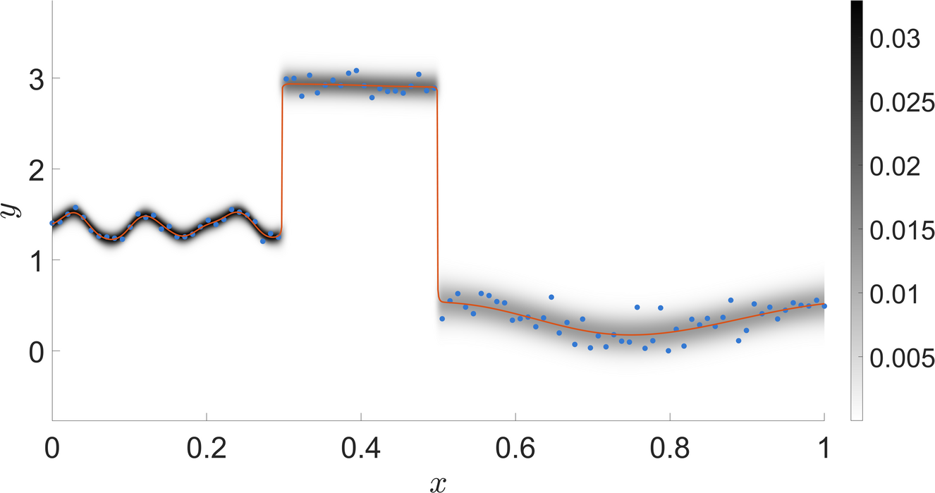
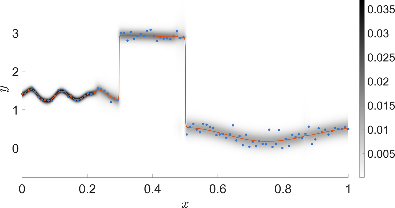
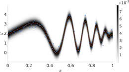
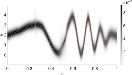
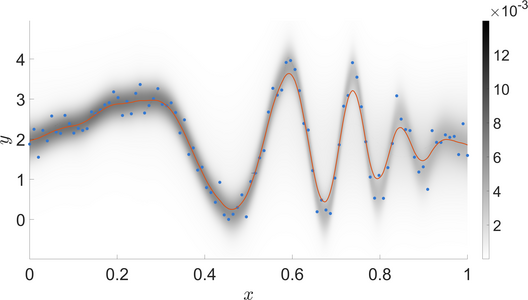
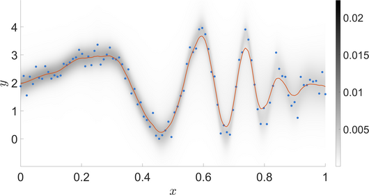
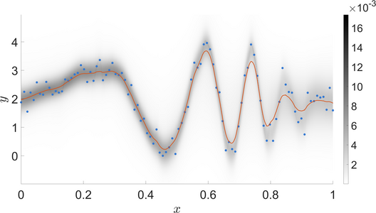
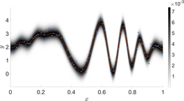
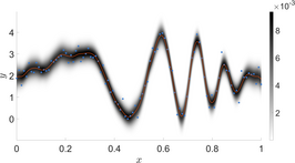
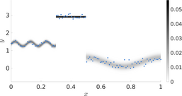
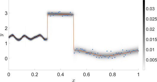
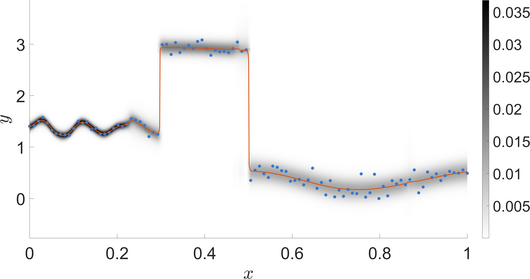
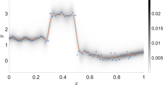
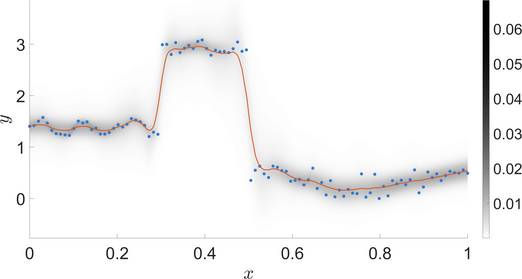
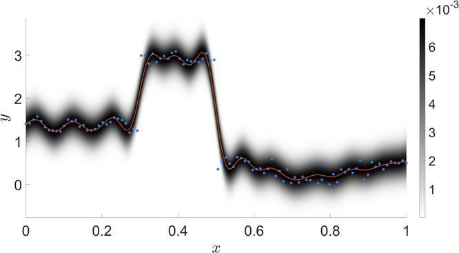
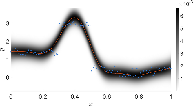
For the synthetic data sets, we present the estimated predictive densities as heat maps in Figures 3 – 4 for both the MoE with SMC² (SMC²-MoE) and the MoE with IS (IS-MoE), along with ground truth and the corresponding results obtained using a single GP, robust Bayesian Committee Machine (RBCM) (Deisenroth and Ng, 2015; Liu et al., 2018), and treedGP (Gramacy, 2007; Gramacy and Lee, 2008; Gramacy and Taddy, 2010). For IS-MoE and SMC²-MoE, we employ an upper bound of $K=7$ experts and consider different choices of the Dirichlet concentration parameter $\alpha=0.1,1,K/2$. In all cases, the number of outer particles $J$, inner particles $M$, and time steps $T$ are chosen so that $MJT^{2}$ is similar to the number of IS samples in order to have similar run times for IS and SMC² and fair comparisons based on a fixed computational budget. The improvement in the estimated predictive densities with SMC² is clearly evident. For the first data set in Figure 3, IS produces disperse densities that are too wiggly on the left side, while SMC² produces density estimates that better match the ground truth. Both the GP and RBCM, which is designed for distributed inference of a stationary GP model, also provide density estimates that are too wiggly on the left side, due to the non-stationary behavior of the underlying function. Instead, the treedGP, which is a mixture of GP experts with a gating network that partitions the input space into axis-aligned regions, is better able to recover the non-stationary behavior of the true function. However, we note that the treedGP R package (Gramacy, 2007) employs MCMC and thus, comes with an increased computational cost, although the SMC² scheme developed here is general and could be used for other choices of gating networks. In the second dataset, the partition plays a crucial role due to the discontinuous nature of the true function and heteroskedastic noise. As postulated, in this setting, the results of IS-MoE in Figure 4 are quite poor, while SMC²-MoE provides substantial improvements, recovering well the ground truth. The GP and RBCM either under-smooth or over-smooth due to the stationary assumption of the models. The results with treedGP are better but highlight the difficult of inferring the cut-off values determining the treed partition structure. We also show $L^{1}$ and $L^{2}$ vector norms between the computed predictive densities and the ground truth densities and the L1 vector norm between the obtained predictive median and the ground truth median in Tables 3 and 4 for the two synthetic data sets.

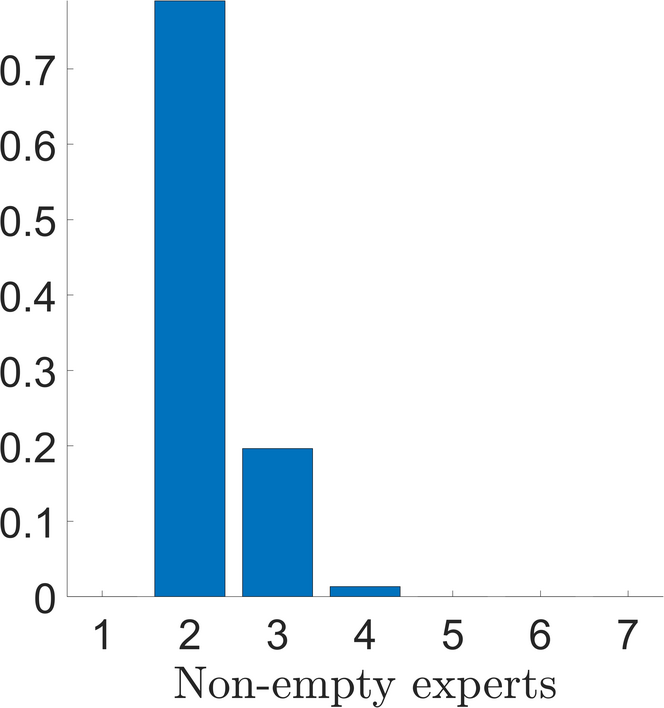
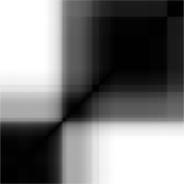
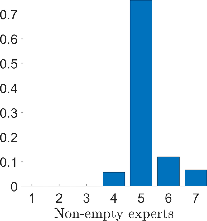
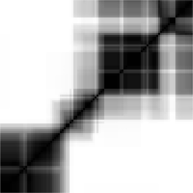
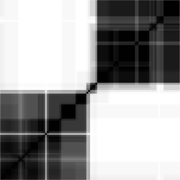
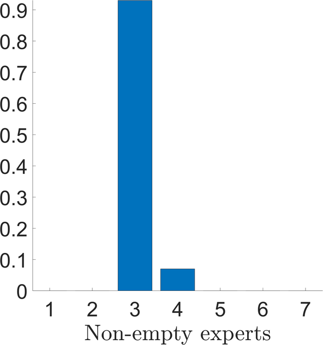
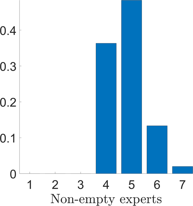
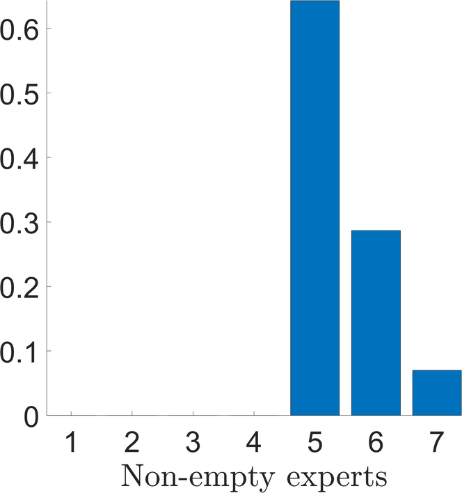
Due to the important role of the partition on predictions, we study and visualize uncertainty in the clustering $C$ by constructing the posterior similarity matrix (PSM) (Gadd et al., 2020). The PSM is an $N$ by $N$ matrix, whose elements represent the posterior probability that two data points are clustered together, i.e. the $ii^{\prime}$th element is given by $p(c_{i}=c_{i^{\prime}}\mid X,Y)$, which is approximated by the weighted average across the particles of the indicators that $c_{i}$ and $c_{i^{\prime}}$ belong to the same expert. For the synthetic data sets, Figures 5–6 illustrate the posterior for the number of non-empty experts (middle column) and the posterior similarity matrices (right column) in comparison to the predicitive density (left column), with rows correpsonding to different values of the Dirichlet concentration parameter $\alpha=0.1,1,K/2$. A smaller value of $\alpha$ encourages sparsity and fewer clusters. In particular, when $\alpha$ is small, we obtain larger clusters, and thus increased computational complexity, but smoother estimates. On the other hand, when $\alpha$ is large, we obtain more clusters of small sizes and reduced computational costs, but estimates tend to be less smooth. In general, we recommend selecting $K$ to be large enough (an upper bound on the number of clusters) and choosing $\alpha$ to balance computational cost and smoothness in the estimates.

Figure 7: Motorcycle data. On the left, the predictive distributions and median are shown in black and red along with the data points in blue for different values of the Dirichlet concentration parameter $\alpha$. In the middle column, the posterior distribution for the number of non-empty experts is shown. The last column shows the posterior similarity matrices summarizing the posterior over partitions. Values of $\alpha=0.1$, $\alpha=1$, and $\alpha=K/2$ are used and correspond to the top, middle, and bottom plots, respectively.

Figure 8: 3D NASA Langley glide-back booster simulation data. On the left, the predictive distributions and median for a one-dimensional slice of the input space are shown in black and red along with the data points in blue for different values of the Dirichlet concentration parameter $\alpha$. In the middle column, the posterior distribution for the number of non-empty experts is shown. The last column shows the posterior similarity matrices summarizing the posterior over partitions. Values of $\alpha=2.7$, $\alpha=6.75$, and $\alpha=K/2=13.5$ are used and correspond to the top, middle, and bottom plots, respectively.

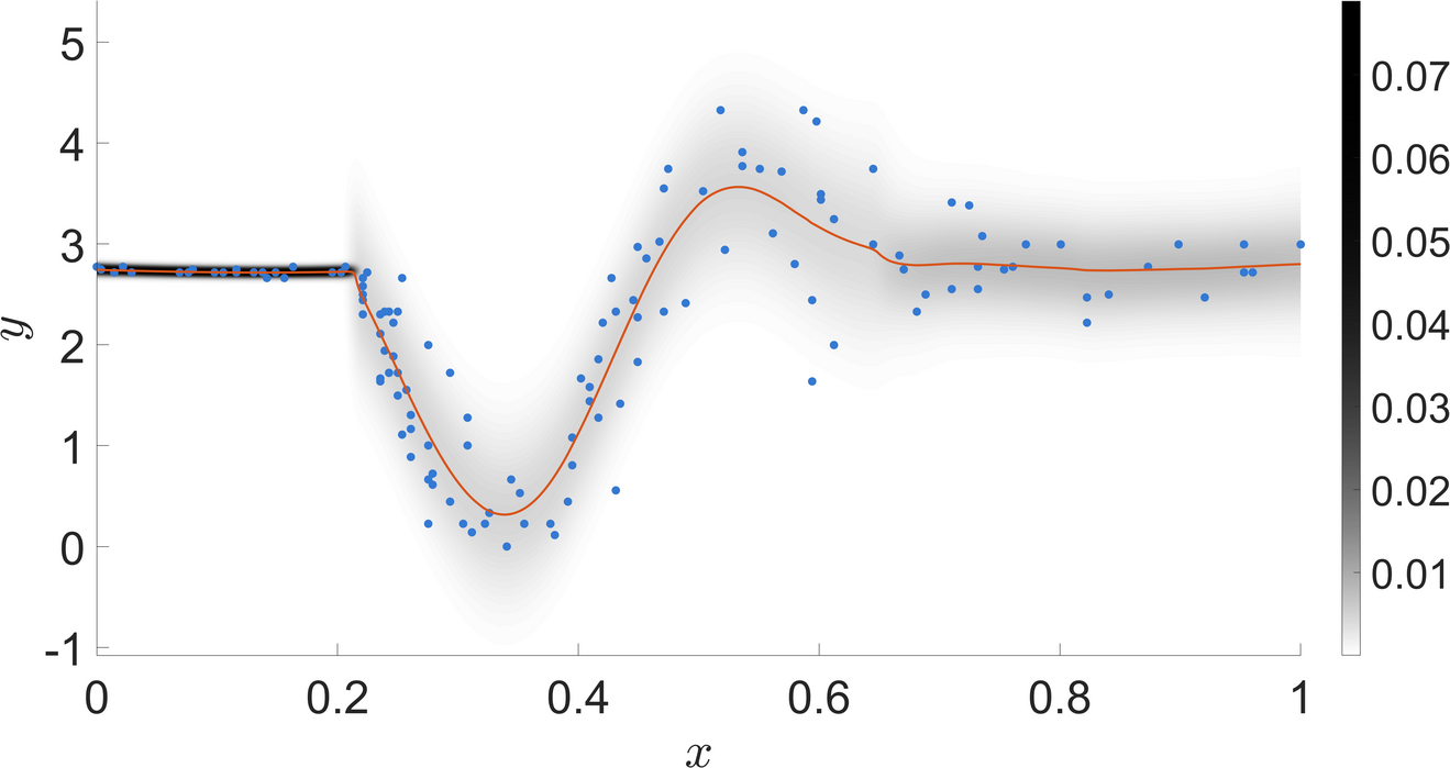
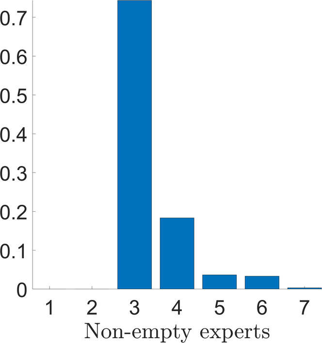
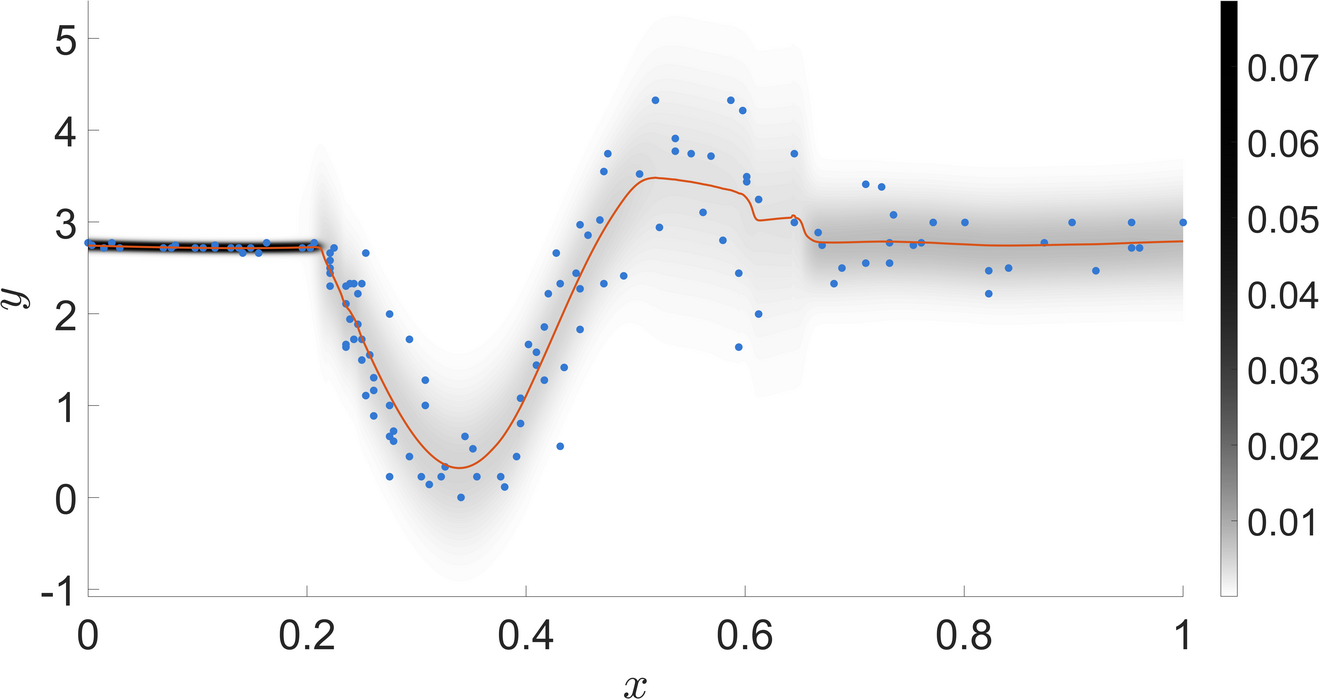
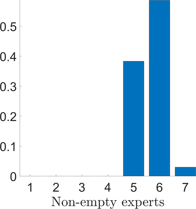
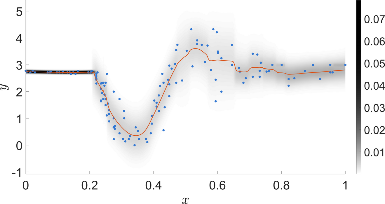
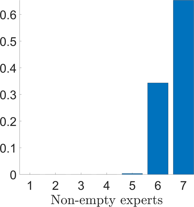
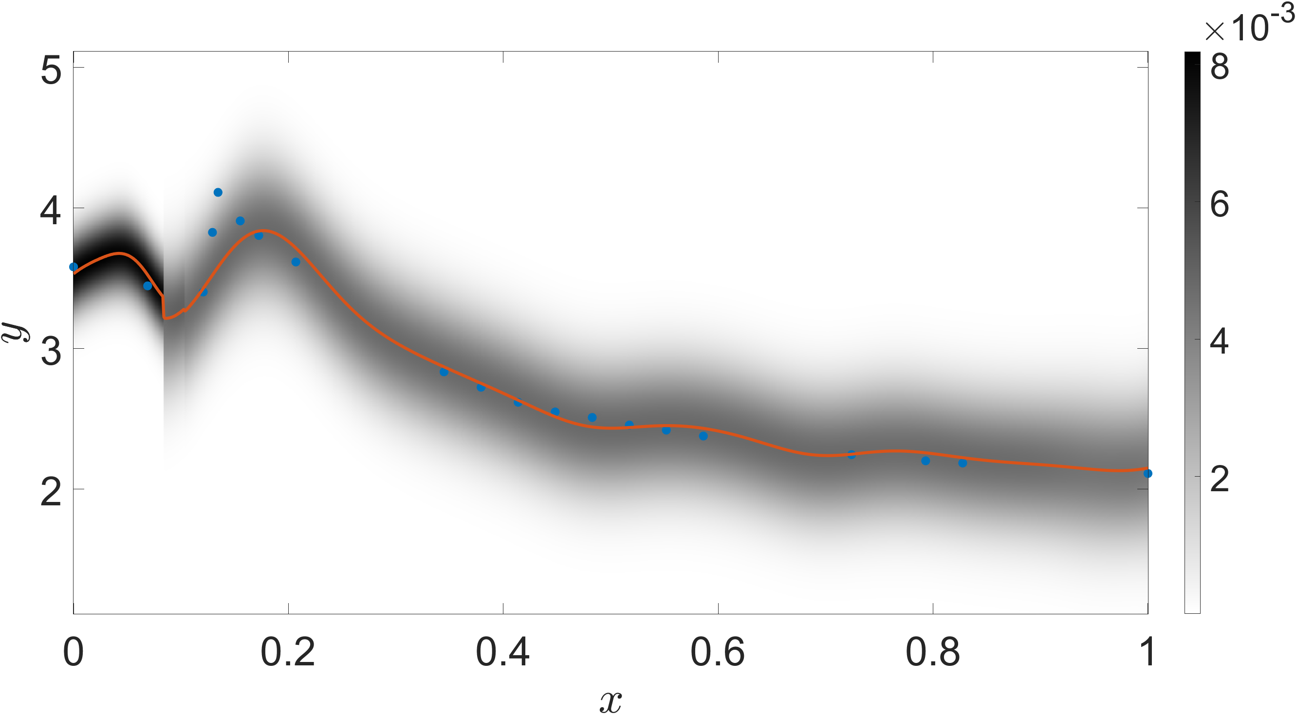
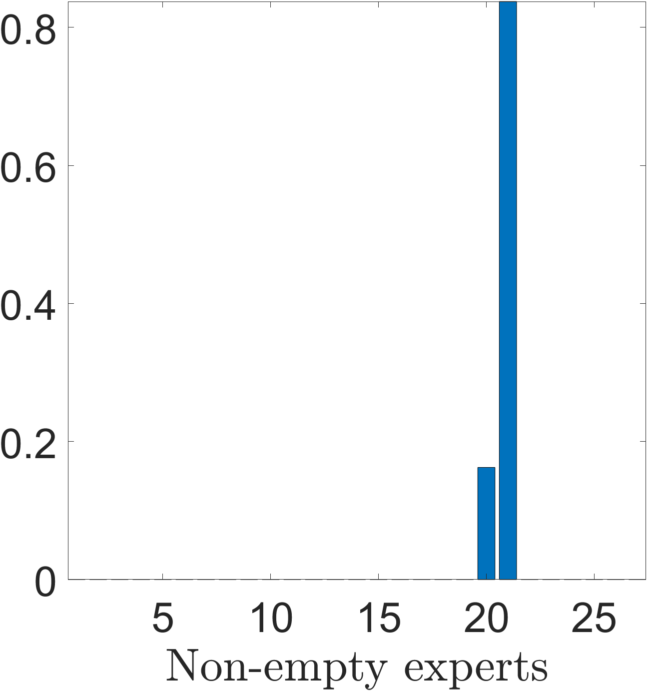
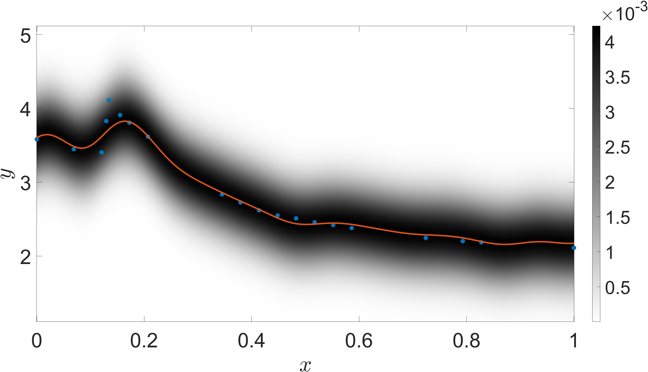
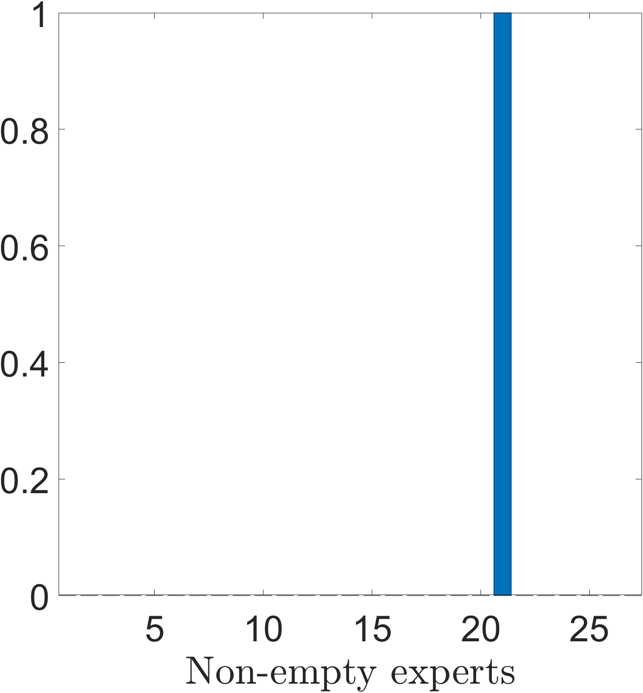
Results for the motorcycle dataset with SMC²-MoE and $K=7$ are provided in Figure 8 and highlight the ability of the model to recover both the non-stationary behavior and heteroskedastic noise present in the data. Rows correspond to different values of the Dirichlet concentration parameter $\alpha$, highlighting the trade-off between sparsity, computational cost, and smoothness. For the NASA data, Figure 7 illustrates the predictive densities for a one-dimensional slice of the input space, along with the posterior over the number of clusters and the posterior similarity matrix for SMC²-MoE and $K=27$. In this case, a larger number of experts and larger value of $\alpha$ are required to capture the ridge at $\text{Mach}=1$ showing the change from subsonic to supersonic flow.

7 Discussion

In this work, we introduced the use of SMC² in the context of mixtures of Gaussian process experts to conduct full Bayesian inference. We have discussed and demonstrated how the previously proposed importance sampling based approach requires the number of importance samples to be exponential in the Kullback-Leibler divergence between the prior and posterior, which is computationally infeasible in many examples. This is particularly true for complex targets that demonstrate departures from standard GP models, such as non-stationarity, heteroskedasticity, and discontinuity. To overcome this, we extended the importance sampling based approach by using nested sequential Monte Carlo samplers to reduce the number of samples required while still being embarrassingly parallel. These benefits offset the additional computational complexity introduced by the nested sequential Monte Carlo samplers, particularly for complex target distributions. The inner SMC can also be replaced by optimization combined with a Laplace approximation to relieve some of the computational burden.

We have focused on gating networks defined through normalized kernels but highlight that the SMC² scheme can also be used for other choices of gating networks. One advantage of this construction is the data-driven choice of the number of clusters, through a sparsity-promoting prior on the weights. Our experiments highlight that the concentration parameter $\alpha$ in the sparsity-promoting prior can be selected to balance sparsity, computational cost, and smoothness.

In future work, we aim to use mixtures of Gaussian process experts as priors for inverse problems such as in computed tomography or deconvolution. In computed tomography, mixtures of Gaussian process could model areas corresponding to differing tissues in the human body or materials in inanimate objects, that is, this would be a flexible alternative to level set methods or edge-preserving priors, such as total variation priors. For deconvolution, mixtures could be used to improve results by enabling modelling of discontinuous functions. In these complex settings, efficient inference schemes for mixtures of GP experts are required.

Acknowledgments

TH and LR were supported by Academy of Finland (grant numbers 327734 and 336787). SW was supported by the Royal Society of Edinburgh (RSE) (grant number 69938).

References

- Andrieu and Roberts (2009) Christophe Andrieu and Gareth O. Roberts. The pseudo-marginal approach for efficient Monte Carlo computations. The Annals of Statistics, 37(2):697–725, 2009.
- Andrieu et al. (2010) Christophe Andrieu, Arnaud Doucet, and Roman Holenstein. Particle Markov chain Monte Carlo methods. Journal of the Royal Statistical Society: Series B (Statistical Methodology), 72(3):269–342, 2010.
- Antoniano-Villalobos et al. (2014) Isadora Antoniano-Villalobos, Sara Wade, and Stephen G. Walker. A Bayesian nonparametric regression model with normalized weights: a study of hippocampal atrophy in Alzheimer’s disease. Journal of the American Statistical Association, 109(506):477–490, 2014.
- Beskos et al. (2014) Alexandros Beskos, Dan Crisan, and Ajay Jasra. On the stability of sequential Monte Carlo methods in high dimensions. The Annals of Applied Probability, 24(4):1396–1445, 2014.
- Bouchard-Côté et al. (2017) Alexandre Bouchard-Côté, Arnaud Doucet, and Andrew Roth. Particle Gibbs split-merge sampling for Bayesian inference in mixture models. Journal of Machine Learning Research, 18(28):1–39, 2017.
- Caron and Doucet (2009) Francois Caron and Arnaud Doucet. Bayesian nonparametric models on decomposable graphs. In Advances in Neural Information Processing Systems, volume 22. Curran Associates, Inc., 2009.
- Carvalho et al. (2010) Carlos M. Carvalho, Hedibert F. Lopes, Nicholas G. Polson, and Matt A. Taddy. Particle learning for general mixtures. Bayesian Analysis, 5(4):709 – 740, 2010.
- Chatterjee and Diaconis (2018) Sourav Chatterjee and Persi Diaconis. The sample size required in importance sampling. The Annals of Applied Probability, 28(2):1099–1135, 2018.
- Chopin (2002) Nicolas Chopin. A sequential particle filter method for static models. Biometrika, 89(3):539–552, 2002.
- Chopin and Papaspiliopoulos (2020) Nicolas Chopin and Omiros Papaspiliopoulos. An Introduction to Sequential Monte Carlo, pages 357–370. Springer International Publishing, 2020.
- Chopin et al. (2013) Nicolas Chopin, Pierre E. Jacob, and Omiros Papaspiliopoulos. SMC2: an efficient algorithm for sequential analysis of state space models. Journal of the Royal Statistical Society: Series B (Statistical Methodology), 75(3):397–426, 2013.
- Consonni and Veronese (2001) Guido Consonni and Piero Veronese. Conditionally reducible natural exponential families and enriched conjugate priors. Scandinavian Journal of Statistics, 28(2):377–406, 2001.
- Deisenroth and Ng (2015) Marc Peter Deisenroth and Jun Wei Ng. Distributed Gaussian processes. In Proceedings of the 32nd International Conference on International Conference on Machine Learning, volume 37, page 1481–1490. JMLR.org, 2015.
- Del Moral et al. (2006) Pierre Del Moral, Arnaud Doucet, and Ajay Jasra. Sequential Monte Carlo samplers. Journal of the Royal Statistical Society: Series B (Statistical Methodology), 68(3):411–436, 2006.
- Denzel and Kästner (2018) Alexander Denzel and Johannes Kästner. Gaussian process regression for geometry optimization. The Journal of Chemical Physics, 148(9):094114, 2018.
- Etienam et al. (2020) Clement Etienam, Kody Law, and Sara Wade. Ultra-fast deep mixtures of Gaussian process experts. arXiv preprint arXiv:2006.13309, 2020.
- Fearnhead (2004) Paul Fearnhead. Particle filters for mixture models with an unknown number of components. Statistics and Computing, 14(1):11–21, 2004.
- Fearnhead and Meligkotsidou (2007) Paul Fearnhead and Loukia Meligkotsidou. Filtering methods for mixture models. Journal of Computational and Graphical Statistics, 16(3):586–607, 2007.
- Filippone et al. (2008) Maurizio Filippone, Francesco Camastra, Francesco Masulli, and Stefano Rovetta. A survey of kernel and spectral methods for clustering. Pattern Recognition, 41(1):176–190, 2008.
- Gadd et al. (2020) Charles Gadd, Sara Wade, and Alexis Boukouvalas. Enriched mixtures of generalised Gaussian process experts. In Proceedings of the Twenty Third International Conference on Artificial Intelligence and Statistics, volume 108, pages 3144–3154. PMLR, 2020.
- Gelman (2006) Andrew Gelman. Prior distributions for variance parameters in hierarchical models (comment on article by Browne and Draper). Bayesian Analysis, 1(3):515 – 534, 2006.
- Gormley and Frühwirth-Schnatter (2019) Isobel Claire Gormley and Sylvia Frühwirth-Schnatter. Mixture of experts models. Handbook of mixture analysis, pages 271–307, 2019.
- Gramacy (2007) Robert B. Gramacy. tgp: An R package for Bayesian nonstationary, semiparametric nonlinear regression and design by treed Gaussian process models. Journal of Statistical Software, 19(9):1–46, 2007.
- Gramacy and Lee (2008) Robert B. Gramacy and Herbert K. H. Lee. Bayesian treed Gaussian process models with an application to computer modeling. Journal of the American Statistical Association, 103(483):1119–1130, 2008.
- Gramacy and Taddy (2010) Robert B. Gramacy and Matthew Taddy. Categorical inputs, sensitivity analysis, optimization and importance tempering with tgp version 2, an R package for treed Gaussian process models. Journal of Statistical Software, 33(6):1–48, 2010.
- Grazian and Robert (2018) Clara Grazian and Christian P. Robert. Jeffreys priors for mixture estimation: properties and alternatives. Computational Statistics & Data Analysis, 121:149–163, 2018.
- Ho et al. (2019) A. Ho, J. Citrin, F. Auriemma, C. Bourdelle, F.J. Casson, Hyun-Tae Kim, P. Manas, G. Szepesi, H. Weisen, and JET Contributors. Application of Gaussian process regression to plasma turbulent transport model validation via integrated modelling. Nuclear Fusion, 59(5):056007, 2019.
- Iikubo et al. (2018) Yuji Iikubo, Shunsuke Horii, and Toshiyasu Matsushima. Sparse Bayesian hierarchical mixture of experts and variational inference. In 2018 International Symposium on Information Theory and Its Applications (ISITA), pages 60–64, 2018.
- Jain and Neal (2004) Sonia Jain and Radford M. Neal. A split-merge Markov chain Monte Carlo procedure for the Dirichlet process mixture model. Journal of Computational and Graphical Statistics, 13(1):158–182, 2004.
- Jasra et al. (2020) Ajay Jasra, Kody Law, and Fangyuan Yu. Unbiased filtering of a class of partially observed diffusions. arXiv preprint arXiv:2002.03747, 2020.
- Jordan and Jacobs (1994) Michael I. Jordan and Robert A. Jacobs. Hierarchical mixtures of experts and the EM algorithm. Neural computation, 6(2):181–214, 1994.
- Li et al. (2011) Feng Li, Mattias Villani, and Robert Kohn. Modeling conditional densities using finite smooth mixtures. Mixtures: estimation and applications, pages 123–144, 2011.
- Liu et al. (2018) Haitao Liu, Jianfei Cai, Yi Wang, and Yew-Soon Ong. Generalized robust Bayesian committee machine for large-scale Gaussian process regression. In Proceedings of Machine Learning Research, volume 80, pages 3131–3140. International Machine Learning Society (IMLS), 2018.
- Lukens et al. (2020) Joseph M. Lukens, Kody J. H. Law, Ajay Jasra, and Pavel Lougovski. A practical and efficient approach for Bayesian quantum state estimation. New Journal of Physics, 22(6):063038, 2020.
- MacEachern et al. (1999) Steven N. MacEachern, Merlise Clyde, and Jun S. Liu. Sequential importance sampling for nonparametric Bayes models: the next generation. The Canadian Journal of Statistics / La Revue Canadienne de Statistique, 27(2):251–267, 1999.
- Mansinghka et al. (2007) Vikash K. Mansinghka, Daniel M. Roy, Ryan Rifkin, and Josh Tenenbaum. Aclass: a simple, online, parallelizable algorithm for probabilistic classification. In Proceedings of Machine Learning Research, volume 2, pages 315–322. PMLR, 2007.
- Masoudnia and Ebrahimpour (2014) Saeed Masoudnia and Reza Ebrahimpour. Mixture of experts: a literature survey. Artificial Intelligence Review, 42(2):275–293, 2014.
- Meeds and Osindero (2005) Edward Meeds and Simon Osindero. An alternative infinite mixture of Gaussian process experts. Advances in neural information processing systems, 18:883–890, 2005.
- Momeni et al. (2020) Ehsan Momeni, Mohammad Bagher Dowlatshahi, Fereydoon Omidinasab, Harnedi Maizir, and Danial Jahed Armaghani. Gaussian process regression technique to estimate the pile bearing capacity. Arabian Journal for Science and Engineering, 45(10):8255–8267, 2020.
- Mossavat and Amft (2011) Iman Mossavat and Oliver Amft. Sparse Bayesian hierarchical mixture of experts. In 2011 IEEE Statistical Signal Processing Workshop (SSP), pages 653–656, 2011.
- Nguyen and Bonilla (2014) Trung Nguyen and Edwin Bonilla. Fast allocation of gaussian process experts. In International Conference on Machine Learning, pages 145–153. PMLR, 2014.
- Norets (2010) Andriy Norets. Approximation of conditional densities by smooth mixtures of regressions. The Annals of Statistics, 38(3):1733–1766, 2010.
- Quinonero-Candela and Rasmussen (2005) Joaquin Quinonero-Candela and Carl Edward Rasmussen. A unifying view of sparse approximate Gaussian process regression. Journal of Machine Learning Research, 6:1939–1959, 2005.
- Quintana et al. (2022) Fernando A Quintana, Peter Müller, Alejandro Jara, and Steven N MacEachern. The dependent Dirichlet process and related models. Statistical Science, 37(1):24–41, 2022.
- Rasmussen and Ghahramani (2002) Carl E. Rasmussen and Zoubin Ghahramani. Infinite mixtures of Gaussian process experts. In Advances in Neural Information Processing Systems 14, pages 881–888. MIT Press, 2002.
- Richardson et al. (2017) Robert R. Richardson, Michael A. Osborne, and David A. Howey. Gaussian process regression for forecasting battery state of health. Journal of Power Sources, 357:209–219, 2017.
- Rousseau and Mengersen (2011) Judith Rousseau and Kerrie Mengersen. Asymptotic behaviour of the posterior distribution in overfitted mixture models. Journal of the Royal Statistical Society: Series B (Statistical Methodology), 73(5):689–710, 2011.
- Särkkä (2013) Simo Särkkä. Bayesian Filtering and Smoothing. Cambridge University Press, 2013.
- Silverman (1985) Bernard W. Silverman. Some aspects of the spline smoothing approach to non-parametric regression curve fitting. Journal of the Royal Statistical Society. Series B (Methodological), 47(1):1–52, 1985.
- Titsias and Likas (2002) Michalis K. Titsias and Aristidis Likas. Mixture of experts classification using a hierarchical mixture model. Neural Computation, 14(9):2221–2244, 2002.
- Tresp (2001) Volker Tresp. Mixtures of Gaussian processes. Advances in neural information processing systems, pages 654–660, 2001.
- Ulker et al. (2010) Yener Ulker, Bilge Günsel, and Taylan Cemgil. Sequential Monte Carlo samplers for Dirichlet process mixtures. In Proceedings of the Thirteenth International Conference on Artificial Intelligence and Statistics, volume 9, pages 876–883. PMLR, 2010.
- Villani et al. (2012) Mattias Villani, Robert Kohn, and David J Nott. Generalized smooth finite mixtures. Journal of Econometrics, 171(2):121–133, 2012.
- Wakabayashi et al. (2018) Yuki K. Wakabayashi, Takuma Otsuka, Yoshitaka Taniyasu, Hideki Yamamoto, and Hiroshi Sawada. Improved adaptive sampling method utilizing Gaussian process regression for prediction of spectral peak structures. Applied Physics Express, 11(11):112401, 2018.
- Williams and Rasmussen (2006) Christopher KI Williams and Carl Edward Rasmussen. Gaussian processes for machine learning, volume 2. MIT press Cambridge, MA, 2006.
- Yu et al. (2022) Weichang Yu, Sara Wade, Howard D Bondell, and Lamiae Azizi. Non-stationary Gaussian process discriminant analysis with variable selection for high-dimensional functional data. Journal of Computational and Graphical Statistics, pages 1–31, 2022.
- Yuan and Neubauer (2008) Chao Yuan and Claus Neubauer. Variational mixture of Gaussian process experts. Advances in Neural Information pProcessing Systems, 21, 2008.
- Zhang and Williamson (2019) Michael Minyi Zhang and Sinead A. Williamson. Embarrassingly parallel inference for Gaussian processes. Journal of Machine Learning Research, 20(169):1–26, 2019.
- İrsoy and Alpaydın (2021) Ozan İrsoy and Ethem Alpaydın. Dropout regularization in hierarchical mixture of experts. Neurocomputing, 419:148–156, 2021.