$I-$Love$-C$ relation for anisotropic neutron star

Abstract

One of the most common assumptions has been made that the pressure inside the star is isotropic in nature. However, the pressure is locally anisotropic in nature which is a more realistic case. In this study, we investigate certain properties of anisotropic neutron stars with the scalar pressure anisotropy model. Different perfect fluid conditions are tested within the star with the relativistic mean-field model equation of states (EOSs). The anisotropic neutron star properties such as mass ($M$), radius ($R$), compactness ($C$), Love number ($k_{2}$), dimensionless tidal deformability ($\Lambda$), and the moment of inertia ($I$) are calculated. The magnitude of the quantities as mentioned above increases (decreases) with the positive (negative) value of anisotropy except $k_{2}$ and $\Lambda$. The Universal relation $I-$Love$-C$ is calculated with almost 58 EOSs spans from relativistic to non-relativistic cases. We observed that the relations between them get weaker when we include anisotropicity. With the help of the GW170817 tidal deformability limit and radii constraints from different approaches, we find that the anisotropic parameter is less than 1.0 if one uses the BL model. Using the universal relation and the tidal deformability bound given by the GW170817, we put a theoretical limit for the canonical radius, $R_{1.4}=10.74_{-1.36}^{+1.84}$ km, and the moment of inertia, $I_{1.4}=1.77_{-0.09}^{+0.17}\times 10^{45}$ g cm² with 90% confidence limit for isotropic stars. Similarly, for anisotropic stars with $\lambda_{\rm BL}=1.0$, the values are $R_{1.4}=11.74_{-1.54}^{+2.11}$ km, $I_{1.4}=2.40_{-0.08}^{+0.17}\times 10^{45}$ g cm² respectively.

I Introduction

Exploration of the internal structure of compact stars such as neutron stars (NS) is one of the most challenging problems because its study involves different areas of physics. Till now, we don’t have a complete theoretical understanding of this object because it has a complex inner structure and strong gravity Lattimer and Prakash (2004). Besides this, we take another realistic phenomenon inside the compact objects termed pressure anisotropy. One of the most common assumptions in studying a neutron star’s equilibrium structure is that its pressure is isotropic. However, the exact case is different due to some exotic process that happens inside it (for a review, see Herrera and Santos (1997)). For example, very high magnetic field Yazadjiev (2012); Cardall et al. (2001); Ioka and Sasaki (2004); Ciolfi et al. (2010); Ciolfi and Rezzolla (2013); Frieben and Rezzolla (2012); Pili et al. (2014); Bucciantini et al. (2015), pion condensation Sawyer (1972), phase transitions Carter and Langlois (1998), relativistic nuclear interaction Canuto (1974); Ruderman (1972), crystallization of the core Nelmes and Piette (2012), superfluid core Kippenhahn Rudolf (1990); Glendenning (1997); Heiselberg and Hjorth-Jensen (2000), etc., are the main cause of the anisotropy inside a star.

A diversity of anisotropic models in literature have been constructed for the matter with a perfect fluid. Mainly Bowers-Liang (BL)  Bowers and Liang (1974), Horvat et al.  Horvat et al. (2010), Cosenza et al.  Cosenza et al. (1981) models have been proposed. The BL model is based on the assumptions that (i) the anisotropy should vanish quadratically at the origin, (ii) the anisotropy should depend non-linearly on radial pressure, and (iii) the anisotropy is gravitationally induced. Horvat et al. proposed that anisotropy is due to the quasi-local equation as given in Ref.  Horvat et al. (2010). Different studies put the limit of anisotropic parameter for e.g., $-2\leq\lambda_{\rm BL}\leq+2$ for BL model  Silva et al. (2015), $-2\leq\lambda_{\rm H}\leq+2$  Doneva and Yazadjiev (2012) for Horvat model. In the present case, we take the BL model, which is explained in the following subsection.

Several studies explained the effects of anisotropic pressure on the macroscopic properties of the compact objects, such as its mass, radius, moment of inertia, tidal deformability, non-radial oscillation  Hillebrandt and Steinmetz (1976); Bayin (1982); Roupas (2021); Deb et al. (2021); Estevez-Delgado and Estevez-Delgado (2018); Pattersons and Sulaksono (2021); Rizaldy et al. (2019); Rahmansyah et al. (2020); Rahmansyah and Sulaksono (2021); Herrera et al. (2008); Herrera and Barreto (2013); Doneva and Yazadjiev (2012); Biswas and Bose (2019); Das et al. (2021a); Roupas and Nashed (2020); Sulaksono (2015); Rahmansyah, A. et al. (2020); Setiawan and Sulaksono (2019); Silva et al. (2015). In general, it is observed that with increasing the magnitude of the anisotropy parameter, the magnitudes of macroscopic properties increase and vice-versa. Contrary to mass and radius, the oscillation frequency of the anisotropic NS decreases Doneva and Yazadjiev (2012). In Ref.  Roupas (2021), it was suggested that the secondary component might be an anisotropic NS, contradicted in Rahmansyah and Sulaksono (2021). Deb et al.  Deb et al. (2021) have claimed that with increasing anisotropy, the star with a transverse magnetic field becomes more massive, increasing the star’s size and vice-versa for the radial field. Using the Skyrme model, Silva et al.  Silva et al. (2015) claimed that the observations of the binary pulsar might constraint the degree of anisotropy. Using GW170817 tidal deformability constraint, Biswas and Bose  Biswas and Bose (2019) observed that a certain equation of state (EOS) becomes viable if the star has enough amount of anisotropy without the violation of causality. In Ref. Rahmansyah and Sulaksono (2021), it has been observed that not only the BL model but the Horvat model is also well consistent with recent multimessenger constraints  Rahmansyah and Sulaksono (2021).

In this study, we calculate the NS properties for different degrees of anisotropy with the modern EOSs. Existing Universal relations are explored between different anisotropic NS properties such as the moment of inertia ($I$), tidal deformability (Love), and compactness ($C$) ($I-$Love$-C$) by varying anisotropic parameters. Yagi and Yunes first obtained the Universal relation for the $I-$Love$-Q$ (where $Q$ is the quadrupole moment) for the slowly rotating and tidally deformed NS Yagi and Yunes (2013) and also for anisotropic NS Yagi and Yunes (2015). Several studies have been dedicated to explaining the Universal relations between different macroscopic properties of the compact objects  Yagi and Yunes (2013, 2015); Gupta et al. (2017); Jiang et al. (2020); Yeung et al. (2021); Chakrabarti et al. (2014); Haskell et al. (2013); Bandyopadhyay et al. (2018). This is because certain physical quantities are found to be interrelated with each other, and the relations are almost independent of the internal structure of the star. Therefore, the EOS insensitive relations are required to decode the information about others, which may not be observationally accessible.

Several studies put constraints on some properties of the NS, such as radius, the moment of inertia (MI), compactness, etc., using the observational data. Lattimer and Schutz constrain the EOSs by measuring MI in the double pulsars system Lattimer and Schutz (2005). Brew and Rezzolla Breu and Rezzolla (2016) have explained some Universal relations for the Keplerian star and also improved the universal relations given by Lattimer and Schutz. This study explains the Universal relation $I-$Love$-C$ for the anisotropic NS. From those relations, we try to constrain the anisotropy parameter with the help of present observational data. Also, we put some theoretical limits on MI, compactness, and radius of both isotropic as well as anisotropic stars.

Exploration of compact star properties needs EOS, which describes the internal mechanism and interactions between different particles present inside the star. The EOS is the relation between pressure and density, which includes all types of interactions occurring inside the star. For this, we use the relativistic mean-field (RMF) model Lalazissis et al. (1997); Furnstahl et al. (1987, 1997, 1996); Dutra et al. (2014); Typel (2005), Skyrme-Hartree-Fock (SHF) model Skyrme (1956, 1958); Chabanat et al. (1998); Dutra et al. (2012), which is non-relativistic in nature. Last few decades, both models played well in different areas of nuclear astrophysics Das et al. (2020, 2021b, 2022); Biswal et al. (2019); Kumar et al. (2017a, 2020). Different systems such as finite nuclei, nuclear matter, and neutron stars where the extended RMF (E-RMF) model is almost well reproduced in their properties Kumar et al. (2017b, 2018); Das et al. (2021c); Kumar et al. (2020). More than two hundred parameter sets have been modeled by the different theoretical groups with either relativistic or non-relativistic approaches. Among them, only a few EOSs have satisfied both nuclear matter properties and reproduced the latest massive NS mass, radius, and tidal deformability called the consistent model  Dutra et al. (2012, 2014); Lourenço et al. (2019).

In this study, we choose RMF unified EOSs for $npe\mu$-matter are BKA24, FSU2, FSUGarnet, G1, G2, G3, GL97, IOPB, IUFSU, IUFSU^∗, SINPA, SINPB, TM1 with standard nonlinear interactions and higher-order couplings from the Parmar et al.  Parmar et al. (2022). Other unified EOSs are taken from the Fortin et al.  Fortin et al. (2017) are the hyperonic $npe\mu Y$-matter variants BSR2Y, BSR6Y, GM1Y, NL3Y, NL3Yss, NL3$\omega\rho$Y, NL3$\omega\rho$Yss, DD2Y, and DDME2Y; the density-dependent linear models such as DD2, DDH$\delta$, and DDME2, and the SHF $npe\mu$-matter models BSk20, BSk21, BSk22, BSk23, BSk24, BSk25, BSk26, KDE0v1, Rs, SK255, SK272, SKa, SKb, SkI2, SkI3, SkI4, SkI5, SkI6, SkMP, SKOp, SLY230a, SLY2, SLY4, and SLY9. All the EOSs are able to reproduced the mass of the NS $\sim 2M_{\odot}$. With these EOSs, we calculate the anisotropic star properties and calculate the $I-$Love$-C$ relations by varying anisotropy parameters. We use the value of $G$ and $c$ as equal to 1 in this calculation.

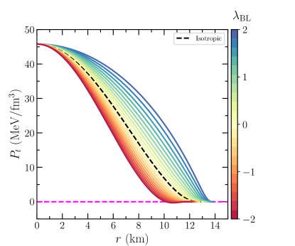
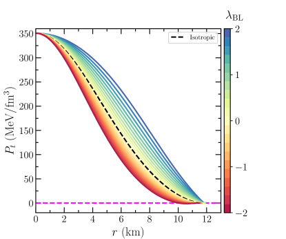
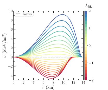
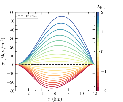
Figure 1: Upper: The tangential pressure as a function of radius profile of a star with different $\lambda_{\rm BL}$ both for canonical (left) and maximum mass (right) of the NS corresponds to IOPB-I EOS. The black dashed line for the isotropic case. Lower: The anisotropy parameter as a function of radius profile.

II Anisotropic configurations

We consider a static and spherically symmetric equilibrium distribution of matter. The stress-energy tensor is defined as Walecka (1974)

$$T_{\mu\nu}=({\cal{E}}+P)u_{\mu}u_{\nu}+Pg_{\mu\nu},$$ (1)

where ${\cal{E}}$ and $P$ are the energy density and pressure of the fluid. The $u_{\mu}$ is the 4-velocity of the fluid respectively.

The anisotropy of the fluid means when the radial pressure ($P_{r}$) differs from the tangential pressure ($P_{t}$). The stress-energy tensor for the corresponding star is defined as  Doneva and Yazadjiev (2012); Silva et al. (2015); Estevez-Delgado and Estevez-Delgado (2018)

$$T_{\mu\nu}=({\cal{E}}+P_{t})u_{\mu}u_{\nu}+(P_{r}-P_{t})k_{\mu}k_{\nu}+P_{t}g_{\mu\nu},$$ (2)

where $k_{\mu}$ is the unit radial vector ($k^{\mu}k_{\mu}=1$) with $u^{\mu}k_{\mu}=0$.

For a spherically symmetric, non-rotating NS, the metric is defined as

$$ds^{2}=e^{\nu}dt^{2}-e^{\lambda}dr^{2}-r^{2}d\theta^{2}-r^{2}\sin^{2}\theta d\varphi^{2}\,.$$ (3)

For an anisotropic NS, the modified Tolman-Oppenheimer-Volkoff (TOV) equations can be obtained by solving Einstein’s equations as  Doneva and Yazadjiev (2012)

$$\frac{dP_{r}}{dr}=-\frac{\left({\cal E}+P_{r}\right)\left(m+4\pi r^{3}P_{r}\right)}{r\left(r-2m\right)}+\frac{2}{r}(P_{t}-P_{r})\,,$$ (4)

$$\frac{dm}{dr}=4\pi r^{2}{{\cal E}}\,,$$ (5)

where the anisotropy parameter is defined as, $\sigma=P_{t}-P_{r}$. The ‘$m$’ is the enclose mass corresponding to radius $r$. Two separate EOSs for $P_{r}$ and $P_{t}$ are needed to solve these TOV equations. We consider the EOS for radial pressure $P_{r}({\cal E})$ from the RMF, SHF, and density-dependent (DD-RMF) models. For transverse pressure ($P_{t}$), we take BL model given in the following Bowers and Liang (1974)

$$P_{t}=P_{r}+\frac{\lambda_{\rm BL}}{3}\frac{({\cal E}+3P_{r})({\cal E}+P_{r})r^{2}}{1-2m/r}\,,$$ (6)

where the factor $\lambda_{\rm BL}$ measures the degree of anisotropy in the fluid.

The TOV equations can be solved using the boundary conditions $r=0,m=0,P_{r}=P_{c}$, and $r=R,m=M,\ {\rm and}\ P_{r}=0$ for a particular choice of anisotropy. The following conditions must be satisfied for the anisotropic NS for a perfect fluid are Estevez-Delgado and Estevez-Delgado (2018); Setiawan and Sulaksono (2019)

1. The pressure and energy density inside the star must be positive, $P_{r},P_{t},\ {\rm and}\ {\cal{E}}>0$.

2. The gradient of radial pressure and energy density must be monotonically decreasing, $\frac{dP_{r}}{dr},\ {\rm and}\ \frac{d{\cal{E}}}{dr}<0$ and maximum value at the centre.

3. The anisotropic fluid configurations with different conditions such as the null energy (${\cal{E}}>0$), the dominant energy (${\cal{E}}+P_{r}>0$, ${\cal{E}}+P_{t}>0$), and the strong energy (${\cal{E}}+P_{r}+2P_{t}>0$) must be satisfied inside the star.

4. The speed of sound inside the star must obey, $0<c_{s,r}^{2}<1$, and $0<c_{s,t}^{2}<1$, where $c_{s}^{2}=\frac{\partial P}{\partial{\cal{E}}}$.

5. The radial and transverse pressure must be the same at the origin.

We check all the above-mentioned conditions, which are well satisfied in this present case, and some of the results are shown in Figs. 1-2 for IOPB-I parameter set.

The transverse pressure as a function of radius is shown in the upper panel of Fig. 1 for a fixed central density. We observe that the value of $P_{t}$ increases with increasing $\lambda_{\rm BL}$, which supports a more massive NS and vice-versa. At the center, both values of $P_{r}$ and $P_{t}$ are the same, which satisfies the above-mentioned condition. At the surface part, the positive values of $\lambda_{\rm BL}$ provide a positive value of $P_{t}$ and vice-versa. This negative value gives the unphysical solutions mainly at the surface part. A more clear picture of the magnitude of the anisotropy parameter can be seen in the lower panel of Fig. 1 for both canonical and maximum mass NS. The magnitude of negativeness increases for the maximum star compared to the canonical star.

The speed of sound $\left(c_{s,t}^{2}=\frac{\partial P_{t}}{\partial{\cal{E}}}\right)$ as a function of radius is depicted in Fig. 2. The $c_{s,t}^{2}$ satisfies the causality limit in the whole region of the star except at the surface part for the negative $\lambda_{\rm BL}$. The transverse pressure and compactness increase with increasing $\lambda_{\rm BL}$ for a star. In Ref. Biswas and Bose (2019), it has been argued that the black hole limit ($C=0.5$) is not possible to achieve by increasing the degree of anisotropy with $\lambda_{\rm BL}=4.0$ for DDH$\delta$ EOS. But at the higher central density, the transverse pressure becomes acausal. We also observed similar results for the IOPB-I EOS with $\lambda_{\rm BL}>4.0$.

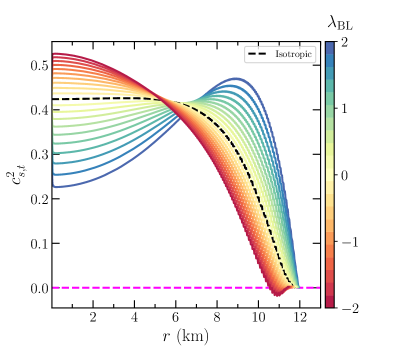
Figure 2: The speed of sound as a function of radius profile of a star with different $\lambda_{\rm BL}$ for the maximum mass of the NS corresponds to IOPB-I EOS.

The mass-radius profiles of the anisotropic NS are solved for IOPB-I EOS for different values of $\lambda_{\rm BL}$, which is shown in Fig. 3. The positive values of $\lambda_{\rm BL}$ increase the maximum masses and their corresponding radii and vice-versa. Different observational data such as x-ray, NICER, and GW can constrain the degree of anisotropy inside the NS. Recently, the fastest and heaviest Galactic NS named PSR J0952-0607 in the disk of the Milky Way has been detected to have mass $M=2.35\pm 0.17\,M_{\odot}$. We also put this limit to constraint the amount of anisotropy.

The GW190814 event raised a debatable issue: Whether the secondary component is the lightest black hole or the heaviest neutron star? Several approaches are already provided in the literature to explain this behavior Fattoyev et al. (2020); Das et al. (2021d); Huang et al. (2020); Roupas (2021); Lim et al. (2021). However, in Ref. Roupas (2021), they claimed that the secondary component might be an anisotropic NS. Therefore, we put the secondary component mass limit $M=2.50-2.67\ M_{\odot}$ in the mass-radius diagram to check whether it reproduced the limit for anisotropy stars within the BL model. We also find that for $\lambda_{\rm BL}=1.8-2$ reproduce the mass $\sim 2.50-2.67M_{\odot}$ but those values of $\lambda_{\rm BL}$ don’t obey the new NICER constraints Miller et al. (2021). In our case, the $-0.4<\lambda_{\rm BL}<+0.4$ almost agrees with the latest observational data.

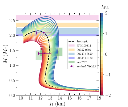
Figure 3: Mass-radius profiles for anisotropic NS with $-2.0<\lambda_{\rm BL}<+2.0$ for IOPB-I EOS. Different color bands signify the masses of the NS observed from the various pulsars, such as PSR J0348+0432 Antoniadis et al. (2013), PSR J0740+6620 Fonseca et al. (2021), heaviest pulsars J0952-0607 Romani et al. (2022) and GW190814 Abbott et al. (2020). The NICER results are shown with two green boxes from two different analyses  Miller et al. (2019); Riley et al. (2019). The revised NICER results are also shown for the canonical star and $2.08\ M_{\odot}$ (red horizontal error bars) given by Miller et al.  Miller et al. (2021).

III Moment of Inertia

For a slowly rotating NS, the system’s equilibrium position can be obtained by solving Einstein’s equation in the Hartle-Throne metric as  Hartle (1967); Hartle and Thorne (1968); Hartle (1973).

$$ds^{2}= -e^{2\nu}\ dt^{2}+e^{2\lambda}\ dr+r^{2}\ (d\theta^{2}+\sin^{2}\theta d\phi^{2})$$ (7)

$$-2\omega(r)r^{2}\sin^{2}\theta\ dt\ d\phi$$

The MI of the slowly rotating anisotropic NS was calculated in Ref.  Rahmansyah, A. et al. (2020)

$$I =\frac{8\pi}{3}\int_{0}^{R}\frac{r^{5}J\tilde{\omega}}{r-2M}({\cal{E}}+P)\left[1+\frac{\sigma}{{\cal{E}}+P}\right]\,dr,$$ (8)

where $\tilde{\omega}=\bar{\omega}/\Omega$, where $\bar{\omega}$ is the frame dragging angular frequency, $\bar{\omega}=\Omega-\omega(r)$. $J$ is defined as $e^{-\nu}(1-2m/r)^{1/2}$. The $\sigma=P_{t}-P_{r}=\frac{\lambda_{\rm BL}}{3}\frac{({\cal E}+3P_{r})({\cal E}+P_{r})r^{2}}{1-2m/r}$. Hence Eq. (8), can be rewritten using Eq. (6) as

$$I =\frac{8\pi}{3}\int_{0}^{R}\frac{r^{5}J\tilde{\omega}}{r-2M}({\cal{E}}+P)\left[1+\frac{\frac{\lambda_{\rm BL}}{3}\frac{({\cal E}+3P)({\cal E}+P)r^{2}}{1-2m/r}}{{\cal{E}}+P}\right]\,dr,$$ (9)

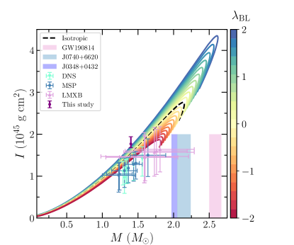
Figure 4: The moment of inertia of the NS as the function of mass. The error bars are taken from the different pulsars analyses as done in Ref. Kumar and Landry (2019). We also put the canonical MI, $I_{1.4}=1.77_{-0.09}^{+0.17}\times 10^{45}$ g cm² obtained in this study for the isotropic star case only.

The obtained values of MI for anisotropic NS are shown in Fig. 4 for IOPB-I EOS. The MI of the NS increases with the mass of the NS. Once the stable configuration is achieved, the MI starts to decrease. The anisotropic effects are clearly seen from the figure for different values of $\lambda_{\rm BL}$. The error bars represent the MI constraints of the different systems such as double neutron stars (DNS), milli-second pulsars (MSP), and low-mass x-ray binaries (LMXB) inferred by Kumar and Landry  Kumar and Landry (2019). Almost all $I\sim M$ curves satisfy these constraints.

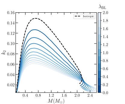
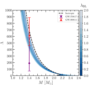
Figure 5: Left: The tidal Love number as a function of mass for different $\lambda_{\rm BL}$ corresponds to IOPB-I EOS. Right: The dimensionless tidal deformability as a function of mass for different $\lambda_{\rm BL}$ corresponds to IOPB-I EOS. The error bars are the observational constraints given by LIGO/Virgo events GW170817 (NS-NS merger)  Abbott et al. (2017) and GW190814 (assuming BH-NS merger)  Abbott et al. (2020).

IV Tidal Deformability

The shape of the NS is deformed when it is present in the external field ($\epsilon_{ij}$) of its companion. Hence the stars develop the quadrupole moment ($Q_{ij}$), which is linear dependent on the tidal field and is defined as  Hinderer (2008, 2009)

$$Q_{ij}=-\lambda\epsilon_{ij}\,,$$ (10)

where $\lambda$ is defined as the tidal deformability of a star. It has relation to the dimensionless tidal Love number $k_{2}$ as $\lambda=\frac{2}{3}k_{2}R^{5}$, where $R$ is the radius of the star.

To determine $k_{2}$, we use the linear perturbation in the Throne and Campolattaro metric Thorne and Campolattaro (1967). We have solved the Einstein equation and obtained the following second-order differential equation for the anisotropic star Biswas and Bose (2019)

$$H^{{}^{\prime\prime}} +H^{{}^{\prime}}\bigg{[}\frac{2}{r}+e^{\lambda}\left(\frac{2m(r)}{r^{2}}+4\pi r(P-{\cal E})\right)\bigg{]}$$

$$+H\left[4\pi e^{\lambda}\left(4{\cal E}+8P+\frac{{\cal E}+P}{dP_{t}/d{\cal E}}(1+c_{s}^{2})\right)-\frac{6e^{\lambda}}{r^{2}}-{\nu^{\prime}}^{2}\right]$$

$$=0\,.$$ (11)

The term $dP_{t}/d{\cal E}$ represents the change of $P_{t}$ (see Eq. (6) for the $P_{t}$) with respect to energy density for fixed value of $\lambda_{\rm BL}$.

The internal and external solutions to the perturbed variable $H$ at the star’s surface can be matched to get the tidal Love number Damour and Nagar (2009); Hinderer (2008). The value of the tidal Love number can then be calculated using the $y_{2}$, and compactness parameter $C$ is defined as  Hinderer (2008, 2009); Das et al. (2021c).

$$k_{2} =\,\frac{8}{5}C^{5}(1-2C)^{2}\big{[}2(y_{2}-1)C-y_{2}+2\big{]}$$

$$\times\Big{\{}2C\big{[}4(y_{2}+1)C^{4}+2(3y_{2}-2)C^{3}-2(11y_{2}-13)C^{2}$$

$$+3(5y_{2}-8)C-3(y_{2}-2)\big{]}+3(1-2C)^{2}$$

$$\times\big{[}2(y_{2}-1)C-y_{2}+2\big{]}\log(1-2C)\Big{\}}^{-1}\,,$$ (12)

where $y_{2}$ depends on the surface value of $H$ and its derivative

$$y_{2}=\frac{rH^{{}^{\prime}}}{H}\Big{|}_{R}.$$ (13)

The gravito-electric Love number ($k_{2}$) and its dimensionless tidal deformability ($\Lambda=\lambda/M^{5}$) are shown in Fig. 5 for the anisotropic NS. Here, we take the positive values of $\lambda_{\rm BL}$. This is because the higher negative values predict negative transverse pressure, and the solutions are unphysical, as described in Ref.  Biswas and Bose (2019). The anisotropy effects are rather small for lower negative values of $\lambda_{\rm BL}$. Hereafter, we neglect those negative values and take only the positive value of $\lambda_{\rm BL}$.

With the increasing value of $\lambda_{\rm BL}$, the magnitude of $k_{2}$ and its corresponding $\Lambda$ decrease. The GW170817 event put a limit on the $\Lambda_{1.4}=190_{-120}^{+390}$, which discarded many older EOSs. In this case, our IOPB-I EOS satisfies both GW170817 and GW190814 limit ($\Lambda_{1.4}=616_{-158}^{+273}$ under NSBH scenario). For the anisotropic case, all values of $\lambda_{\rm BL}$, the predicted $\Lambda_{1.4}$ are almost in the range of the GW170817, and few higher-order values don’t lie in the GW190814 limit.

For anisotropic NS, the magnitude of $\Lambda_{1.4}$ is lesser than the isotropic case. Hence, the anisotropic NS tidally deformed less and sustained more time in the inspiral-merger process compared to the isotropic case.

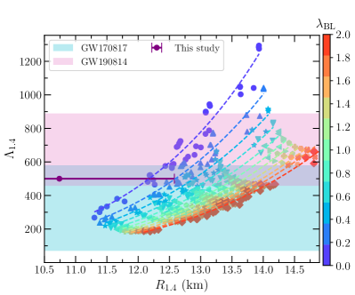
Figure 6: Relation between $\Lambda_{1.4}$ and $R_{1.4}$ with different anisotropy parameter for different EOSs. The dashed lines are fitted using the function $aR_{1.4}^{b}$, where $a$ and $b$ are fitting coefficients. We also put the canonical radius limit, $R_{1.4}=10.74_{-1.36}^{+1.84}$ km obtained in this study for the isotropic star case only.

In Fig. 6, we show the relation between the canonical dimensionless tidal deformability ($\Lambda_{1.4}$) as a function of canonical radius ($R_{1.4}$) for different values of anisotropicity with assumed EOSs. We fit the $\Lambda_{1.4}$ and $R_{1.4}$ with a function $aR_{1.4}^{b}$ for a fix value of $\lambda_{\rm BL}$. The fitting coefficients are given in Table 1. In Ref.  Fattoyev et al. (2018), it is found that the value of $a$ and $b$ are $7.76\times 10^{-4}$ and 5.28 respectively with correlation coefficient $r=0.98$. These coefficients are modified for huge EOSs considerations by Annala et al.  Annala et al. (2018). They found a robust correlation having $a=2.88\times 10^{-6}$ and $b=7.5$. Malik et al. Malik et al. (2018a) found that the values are $9.11\times 10^{-5}$ and 6.13 with 98% correlation.

In this case, we find that $a=2.28\times 10^{-5}$ and $b=6.76$ with correlation coefficients $r=0.948$ for isotropic NS. With the inclusion of anisotropicity, the values of $a$’s are increasing while $b$’s are decreasing. Also, we obtained a more robust correlation for anisotropic NS with higher $\lambda_{\rm BL}$. For example, for isotropic case, the value of $r=0.958$. With increasing $\lambda_{\rm BL}$, the correlations coefficients are 0.967, and 0.973 for $\lambda_{\rm BL}=1.0\,\&\,2.0$ respectively.

Table 1: The fitting coefficients $a$, and $b$ with relation $\Lambda_{1.4}=aR_{1.4}^{b}$ corresponding to different $\lambda_{\rm BL}$.

$\lambda_{\rm BL}$	0.0	1.0	2.0
$a(10^{-5})$	2.28	3.07	3.10
$b$	6.76	6.37	6.25
$r$	0.948	0.967	0.973

V Universal relations

Here, we analyze the different types of Universal relations among the moment of inertia, tidal deformability, and compactness which are already defined. But, here, we mainly focus on the Universal relations for an anisotropic NS. Such approximate Universal relations are quite important for astrophysical observations due to the fact that it breaks the degenerates in the data analysis and model selections for different observations such as x-ray, radio, and gravitational waves Yagi and Yunes (2015).

V.1 $I-\Lambda$ relations

The $I-$Love relation was calculated by Yagi, and Yunes Yagi and Yunes (2013) for slowly rotating NS with few EOSs and also included some polytropic EOSs. Later on, these relations were extended by several works to different systems of anisotropic  Yagi and Yunes (2015); Gupta et al. (2017); Jiang et al. (2020); Yeung et al. (2021); Chakrabarti et al. (2014); Haskell et al. (2013); Bandyopadhyay et al. (2018). Here, we calculate the $I-$Love relations for anisotropic NS.

The MI of the anisotropic NS is calculated using Hartle-Throne approximations. The dimensionless moment of inertia ($\bar{I}=I/M^{3}$) is plotted as the function of dimensionless tidal deformability ($\Lambda$) in Figs. 7-9 with $\lambda_{\rm BL}=0-2$ for anisotropic NS. We fit these relations with the formula given in Refs. Landry and Kumar (2018); Kumar and Landry (2019)

$$\log_{10}\bar{I}=\sum_{n=0}^{4}a_{n}(\log_{10}\Lambda)^{n},$$ (14)

and the coefficients are listed in Table 3. Our fit is almost similar with Yagi & Yunes Yagi and Yunes (2013) and Landry & Kumar Landry and Kumar (2018). But the coefficients are slightly modified due to the anisotropicity. The residuals are computed with the formula.

$$\Delta\bar{I}=\frac{|\bar{I}-\bar{I}_{\rm fit}|}{\bar{I}_{\rm fit}},$$ (15)

with reduced chi-squared ($\chi_{r}^{2}$) errors are also enumerated in Table 3. With increasing the anisotropy, the value of $\chi^{2}$ errors increases, which means the EOS insensitive relations get weaker with the addition of anisotropy.

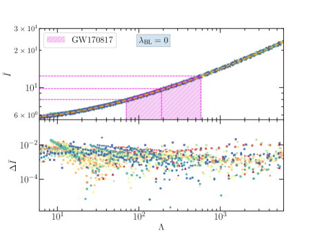
Figure 7: $\bar{I}-\Lambda$ relation with anisotropy parameter $\lambda_{\rm BL}=0$ for assumed EOSs. The orange dashed line is fitted with the Eq. (14). The magenta shaded region is canonical tidal deformability data from the GW170817 paper Abbott et al. (2017). The lower panel are the residuals for the fitting calculated using the formula in Eq. (15).

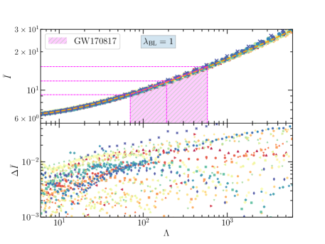
Figure 8: Same as Fig. 7, but with $\lambda_{\rm BL}=1$.

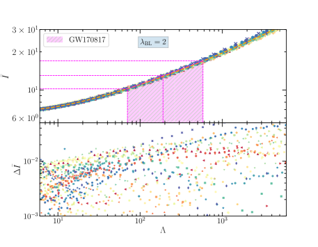
Figure 9: Same as Fig. 7, but with $\lambda_{\rm BL}=2$.

With the help of tidal deformabilities data from the GW170817 and GW190814 events, we put constraints on $\bar{I}$ for isotropic star and found to be $\bar{I}_{1.4}=14.88_{-0.76}^{+1.42},\,{\rm and}\,21.50_{-0.91}^{+1.13}$ respectively (see Table 2). Landry and Kumar Landry and Kumar (2018) obtained the limit is $\bar{I}=11.10_{-2.28}^{+3.64}$. From the GW170817 event, the value of $\Lambda_{1.4}\leq 800$, which put the upper limit, is found to be $\bar{I}\leq 16.07$ Landry and Kumar (2018). The theoretical upper limit for the isotropic case almost matches the GW170818 limit. There are many theoretical limits on the MI of the NS  Moelnvik and Oestgaard (1985); Lattimer and Schutz (2005); Worley et al. (2008); Breu and Rezzolla (2016); Zhao (2017); Lim et al. (2019); Jiang et al. (2020); Greif et al. (2020). The constraints on its value become tighter if we may detect more double pulsars (like PSR J0737-3039) in the near future. For anisotropic cases, the magnitudes for the $\bar{I}$ and $I$ are larger than the isotropic case. Due to anisotropy, the mass of the NS increases, which gives rise to the magnitude of MI.

Table 2: The canonical dimensionless MI ($\bar{I}_{1.4}$), and MI ($I_{1.4}\times 10^{45}$ g cm²) inferred from GW170817 and GW190814 data.

$\lambda_{\rm BL}$	GW170817		GW190814
	$\bar{I}_{1.4}$	$I_{1.4}$	$\bar{I}_{1.4}$	$I_{1.4}$
$0.0$	$14.88_{-0.76}^{+1.42}$	$1.77_{-0.09}^{+0.17}$	$21.50_{-0.91}^{+1.13}$	$2.56_{-0.11}^{+0.14}$
$1.0$	$20.14_{-0.72}^{+1.48}$	$2.40_{-0.08}^{+0.17}$	$30.51_{-0.90}^{+1.15}$	$3.63_{-0.11}^{+0.14}$
$2.0$	$22.99_{-0.72}^{+1.50}$	$2.74_{-0.85}^{+0.18}$	$35.31_{-0.89}^{+1.15}$	$4.20_{-0.11}^{+0.14}$

Table 3: The fitting coefficients are listed for $I-\Lambda$, $C-\Lambda$, and $C-I$ relations with $\lambda_{\rm BL}=0.0,1.0,2.0$. The reduced chi-squared ($\chi_{r}^{2}$) is also given for all cases.

$I-\Lambda$				$C-\Lambda$				$C-I$
$\lambda_{\rm BL}=$	0.0	1.0	2.0	$\lambda_{\rm BL}=$	0.0	1.0	2.0	$\lambda_{\rm BL}=$	0.0	1.0	2.0
$a_{0}(10^{-1})=$	$7.5026$	$7.9782$	$8.3145$	$b_{0}(10^{-1})=$	$3.6873$	$3.4833$	$3.4156$	$c_{0}(10^{-2})=$	$5.2024$	$6.2526$	$7.3034$
$a_{1}(10^{-2})=$	$4.1857$	$5.3001$	$5.6152$	$b_{1}(10^{-2})=$	$-4.1113$	$-4.0443$	$-4.0723$	$c_{1}(10^{-1})=$	$-5.1531$	$-6.0861$	$-7.0385$
$a_{2}(10^{-2})=$	$8.0495$	$10.3482$	$11.1359$	$b_{2}(10^{-3})=$	$1.5301$	$1.5771$	$1.6364$	$c_{2}=$	$1.5903$	$1.87517$	$2.1721$
$a_{3}(10^{-3})=$	$-8.9478$	$-15.3418$	$-18.1670$	$b_{3}(10^{-5})=$	$-1.8874$	$-2.0472$	$-2.1929$	$c_{3}=$	$-1.3667$	$-1.7363$	$-2.1099$
$a_{4}(10^{-4})=$	$5.4767$	$10.9879$	$14.4628$	$b_{4}=$	$---$	$---$	$---$	$c_{4}=$	$0.4289$	$0.6017$	$0.7684$
$\chi_{r}^{2}(10^{-5})=$	$0.4133$	$2.6245$	$4.5281$	$\chi_{r}^{2}(10^{-5})=$	$1.0981$	$0.9022$	$0.8409$	$\chi_{r}^{2}(10^{-4})=$	$0.0948$	$0.8379$	$4.5028$

V.2 $C-\Lambda$ relations

The Universal relation for $C-\Lambda$ for the isotropic star was first pointed out by Maselli et al.  Maselli et al. (2013). Later on, it was extended to anisotropic star by Biswas et al.  Biswas and Bose (2019) for a few EOSs such as SLy4, APR4, WFF1, DDH$\delta$, and GM1 EOSs. We fit the relation between $C$ and $\Lambda$ using Eq. (16) for considered EOSs with $\lambda_{\rm BL}$ varies from 0 to 2 and the fitting coefficients are listed in Table 3. With increasing $\lambda_{\rm BL}$, the magnitude of $b_{n}$ decreases, implying that the fitting is more robust than the isotropic case. The inferred compactness of the isotropic star is more in comparison with the anisotropic star. This signifies that the anisotropic star is less compact than the isotropic one (see Table 4).

We calculate the tidal deformability of the anisotropic NS for the $\lambda_{\rm BL}=0,1,2$ and shown in Figs. 10 - 12. We perform the least-squares fit using the approximate formula.

$$C=\sum_{n=0}^{3}b_{n}(\ln\Lambda)^{n},$$ (16)

where $b_{n}$ are the coefficients of the fitting given in Table 3. The fit residuals are calculated as $\Delta C=|C-C_{\rm fit}|/C_{\rm fit}$ and displayed in the lower panel of Fig. 10.

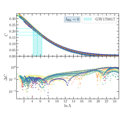
Figure 10: $C-\Lambda$ relation with anisotropy parameter $\lambda_{\rm BL}=0$ for assumed EOSs. The orange dashed line is fitted with the Eq. (16). The orange-shaded region is canonical tidal deformability data from the GW170817 paper Abbott et al. (2017). The lower panel is the residual of the fitting.

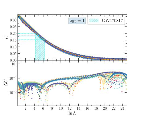
Figure 11: Same as Fig. 10, but with $\lambda_{\rm BL}=1$.

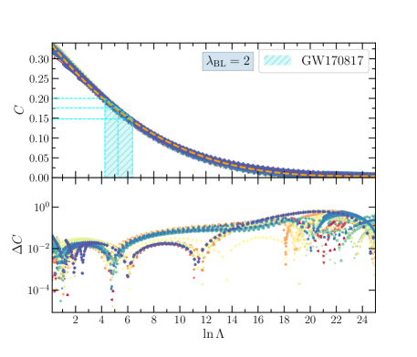
Figure 12: Same as Fig. 10, but with $\lambda_{\rm BL}=2$.

Table 4: The canonical compactness ($C_{1.4}$), and radius ($R_{1.4}$) inferred from GW170817 and GW190814 data.

$\lambda_{\rm BL}$	GW170817		GW190814
	$C_{1.4}$	$R_{1.4}$	$C_{1.4}$	$R_{1.4}$
$0.0$	$0.192_{-0.03}^{+0.03}$	$10.74_{-1.36}^{+1.84}$	$0.163_{-0.01}^{+0.01}$	$12.69_{-0.53}^{+0.71}$
$1.0$	$0.177_{-0.03}^{+0.03}$	$11.74_{-1.54}^{+2.11}$	$0.149_{-0.01}^{+0.01}$	$13.94_{-0.62}^{+0.80}$
$2.0$	$0.169_{-0.03}^{+0.03}$	$12.18_{-1.65}^{+2.27}$	$0.142_{-0.01}^{+0.01}$	$14.58_{-0.66}^{+0.88}$

We infer the values of both compactness and radius of the canonical star with $\Lambda_{1.4}=190_{-120}^{+390}$ given by GW170817  Abbott et al. (2018) and $\Lambda_{1.4}=616_{-158}^{+273}$ by GW190814 Abbott et al. (2020) which are enumerated in Table 4. Several studies put a limit on the canonical radius of the star with different conditions Malik et al. (2018b); Hebeler et al. (2010); Lim and Holt (2018); Most et al. (2018); Fattoyev et al. (2018); Lourenço et al. (2020); Tews et al. (2018); Annala et al. (2018); Zhang et al. (2018); Dietrich et al. (2020); Capano et al. (2020); De et al. (2018); Köppel et al. (2019); Montaña et al. (2019); Radice and Dai (2019); Coughlin et al. (2019); Kumar and Landry (2019). All the radii constraints are listed in Table 2 in Ref. Montaña et al. (2019). Here, we also put the limit on $R_{1.4}$ and $C_{1.4}$ with the help of observational data. It is observed that the highest limit on $R_{1.4}$ is 13.76 km by Fattoyev et al. Fattoyev et al. (2018) using GW170817 data. If we stick to that limit, then our predictions for $R_{1.4}$ are matched for both isotropic and anisotropic with $\lambda_{\rm BL}=1.0$. In case of the lower limit of $R_{1.4}$, the $\lambda_{\rm BL}=0.0$ satisfies the limit given by the Tews et al. Tews et al. (2018), and De et al. De et al. (2018). Hence, it is observed that the anisotropy inside the NS must be less than 1.0 if one uses the BL model.

V.3 $C-I$ relations

The dimensionless MI can be expressed as a function of compactness via lower order polynomial, and it was first pointed out by Ravenhall and Pethick Ravenhall and Pethick (1994). Later on, several authors have studied and modified the same relations for double pulsar system with higher-order polynomial fitting Lattimer and Schutz (2005), scalar-tensor theory and ${\cal R}^{2}$ gravity Staykov et al. (2016); Popchev et al. (2019), rotating stars Breu and Rezzolla (2016), strange stars Bejger, M. and Haensel, P. (2002). In the present case, we study the $C-I$ relations for anisotropic NS.

Brew and Rezzolla explain the universal behavior of dimensionless MI ($I/M^{3}$) is more accurate than the dimensionless MI defined earlier ($I/MR^{2}$). Hence, in this study, we use $I/M^{3}$ rather than $I/MR^{2}$. The compactness and dimensionless MI are related in the following polynomial given as Landry and Kumar (2018); Kumar and Landry (2019)

$$C=\sum_{n=0}^{4}c_{n}(\log_{10}\bar{I})^{-n},$$ (17)

where the $c_{n}$ is the fitting coefficients are listed in Table 3. The relations between them are depicted in Figs. 13 - 15 for different anisotropy. We can put the constraints on the $\bar{I}$ and $C$ from our previous limit as given in Table 2- 4.

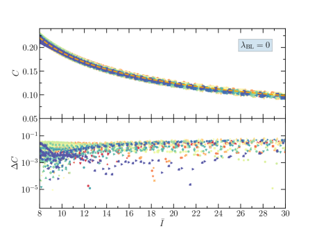
Figure 13: $C-I$ relation with anisotropy parameter $\lambda_{\rm BL}=0$ for assumed EOSs. The orange dashed line is fitted with the Eq. (17). The lower panel is the residual of the fitting.

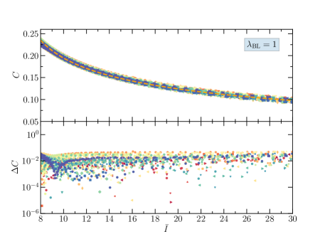
Figure 14: Same as Fig. 13, but with $\lambda_{\rm BL}=1$.

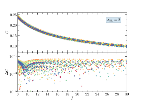
Figure 15: Same as Fig. 13, but with $\lambda_{\rm BL}=2$.

VI Discussions and Conclusion

In this study, we calculate the properties of the anisotropic star based on a simple BL model with 58 parameter sets spanning from relativistic to non-relativistic cases. The macroscopic properties magnitudes such as mass and radius increase due to the anisotropy since an extra contribution comes due to the pressure difference between radial and transverse components. This difference is always model dependent, for example, in the BL and Horvat models. Some of these conditions must be satisfied, such as both transverse and radial pressure, and central energy density must be greater than zero inside the whole star. Extra conditions like null energy, dominant energy, and strong energy are well satisfied inside the whole region of the star. Also, the sound speeds for both components are still valid for the anisotropic stars.

The magnitude of transverse pressure increases by varying $\lambda_{\rm BL}$ for both canonical and maximum mass stars. But the magnitude is greater for the maximum mass case than for the canonical star. Both transverse pressure and the speed of sound at the surface part become negative, which gives the unphysical solution for higher negative values of anisotropy. Therefore, we don’t take such anisotropy cases further in this study. The moment of inertia of the anisotropic star is obtained with a slowly rotating anisotropic star, and it is found that the magnitude increases with anisotropy. Other macroscopic properties, such as tidal Love number and dimensionless tidal deformability, are calculated for the IOPB-I parameter set. We observe that the effects of anisotropy decrease the magnitude of both $k_{2}$ and $\Lambda$. This implies that the star with higher anisotropy sustains more life in the inspiral-merger phase and vice-versa. This is because the star with higher $\Lambda$ deformed more, the merger process accelerates, and the collapse will happen earlier, as described in Ref. Das et al. (2021b). Hence, one should take the anisotropy inside the NS to theoretically explore the gravitational waves coming from the binary NS inspiral-merger-ringdown phase.

This study calculates the Universal relation $I-$Love$-C$ for the anisotropic star. The Universal relations are mainly required to extract information about the star properties, which doesn’t become accessible to detect by our detectors/telescopes. The Universal relations such as $I-\Lambda$, $C-\Lambda$, and $C-I$ are calculated by changing the anisotropy value. We fit all the relations with a polynomial fit using the least-square method. Our coefficients are almost on par with the different approaches available in the literature. We find that the reduced chi-square errors for $I-\Lambda$, $C-\Lambda$, and $C-I$ are $0.4133\times 10^{-5}$, $1.0981\times 10^{-5}$ and $0.0948\times 10^{-4}$ respectively for isotropic star. With anisotropy $\lambda_{\rm BL}=1.0$, the errors are $2.6245\times 10^{-5}$, $0.9022\times 10^{-5}$ and $0.8379\times 10^{-4}$ respectively. The sensitiveness of the Universal relations such as $I-\Lambda$ and $C-I$ are weaker for the anisotropic star in comparison with the isotropic star. But we obtain the relation between $C-\Lambda$ gets stronger with increasing anisotropy.

We constraint the value of anisotropy using the obtained Universal relations from the GW170817 data and find that the value of $\lambda_{\rm BL}$ is less than 1.0 if one uses the BL model. The canonical radius, compactness, and moment of inertia are found to be $10.74_{-1.36}^{+1.84}$ km, $0.192\pm 0.03$, $14.88_{-0.76}^{+1.42}$ respectively for the isotropic star. For an anisotropic star, the magnitudes of both the canonical radius and the MI increase, but canonical compactness decreases. From the various canonical radius constraints inferred from the GW170817 data, we enumerated the radius of the anisotropic star is less than the $R_{1.4}=13.85$ km if one uses the BL model. This limit can be modified with different anisotropy models by including phenomena like a magnetic field, quark inside the core, dark matter, etc., in detail. Hence, one can check the different aspects which may produce the anisotropy inside the compact stars and can constraint its degree with the help of observational data.

VII ACKNOWLEDGMENTS

I would like to thank Prof. P. Landry and Prof. Bharat Kumar for the discussions on the fitting procedures and also like to thank Prof. A. Sulaksono for formulating the moment of inertia for the anisotropic star. I am extremely thankful to my supervisor Prof. S. K. Patra, for the constant support during this project and for carefully reading the manuscript. I also want to thank Ankit Kumar, Jeet Amrit Pattnaik, and Vishal Parmar for the discussions during this project.

References

- Lattimer and Prakash (2004) J. M. Lattimer and M. Prakash, Science 304, 536 (2004).
- Herrera and Santos (1997) L. Herrera and N. Santos, Physics Reports 286, 53 (1997).
- Yazadjiev (2012) S. S. Yazadjiev, Phys. Rev. D 85, 044030 (2012).
- Cardall et al. (2001) C. Y. Cardall, M. Prakash, and J. M. Lattimer, The Astrophysical Journal 554, 322 (2001).
- Ioka and Sasaki (2004) K. Ioka and M. Sasaki, The Astrophysical Journal 600, 296 (2004).
- Ciolfi et al. (2010) R. Ciolfi, V. Ferrari, and L. Gualtieri, Monthly Notices of the Royal Astronomical Society 406, 2540 (2010).
- Ciolfi and Rezzolla (2013) R. Ciolfi and L. Rezzolla, Monthly Notices of the Royal Astronomical Society: Letters 435, L43 (2013).
- Frieben and Rezzolla (2012) J. Frieben and L. Rezzolla, Monthly Notices of the Royal Astronomical Society 427, 3406 (2012).
- Pili et al. (2014) A. G. Pili, N. Bucciantini, and L. Del Zanna, Monthly Notices of the Royal Astronomical Society 439, 3541 (2014).
- Bucciantini et al. (2015) N. Bucciantini, A. G. Pili, and L. Del Zanna, Monthly Notices of the Royal Astronomical Society 447, 3278 (2015).
- Sawyer (1972) R. F. Sawyer, Phys. Rev. Lett. 29, 382 (1972).
- Carter and Langlois (1998) B. Carter and D. Langlois, Nuclear Physics B 531, 478 (1998).
- Canuto (1974) V. Canuto, Annual Review of Astronomy and Astrophysics 12, 167 (1974).
- Ruderman (1972) M. Ruderman, Annual Review of Astronomy and Astrophysics 10, 427 (1972).
- Nelmes and Piette (2012) S. Nelmes and B. M. A. G. Piette, Phys. Rev. D 85, 123004 (2012).
- Kippenhahn Rudolf (1990) W. A. Kippenhahn Rudolf, Stellar Structure and Evolution, Vol. XVI (Springer Berlin, Heidelberg, 1990).
- Glendenning (1997) N. K. Glendenning, Compact stars: Nuclear physics, particle physics, and general relativity (Springer-Verlag New York, 1997).
- Heiselberg and Hjorth-Jensen (2000) H. Heiselberg and M. Hjorth-Jensen, Physics Reports 328, 237 (2000).
- Bowers and Liang (1974) R. L. Bowers and E. P. T. Liang, Astrophys. J. 188, 657 (1974).
- Horvat et al. (2010) D. Horvat, S. Ilijić, and A. Marunović, Classical and Quantum Gravity 28, 025009 (2010).
- Cosenza et al. (1981) M. Cosenza, L. Herrera, M. Esculpi, and L. Witten, J Math Phys (NY) 22, 118 (1981).
- Silva et al. (2015) H. O. Silva, C. F. B. Macedo, E. Berti, and L. C. B. Crispino, Classical and Quantum Gravity 32, 145008 (2015).
- Doneva and Yazadjiev (2012) D. D. Doneva and S. S. Yazadjiev, Phys. Rev. D 85, 124023 (2012).
- Hillebrandt and Steinmetz (1976) W. Hillebrandt and K. O. Steinmetz, Astronomy and Astrophysics 53, 283 (1976).
- Bayin (1982) S. Bayin, Phys. Rev. D 26, 1262 (1982).
- Roupas (2021) Z. Roupas, Astrophysics and Space Science 366, 9 (2021).
- Deb et al. (2021) D. Deb, B. Mukhopadhyay, and F. Weber, The Astrophysical Journal 922, 149 (2021).
- Estevez-Delgado and Estevez-Delgado (2018) G. Estevez-Delgado and J. Estevez-Delgado, The European Physical Journal C 78, 673 (2018).
- Pattersons and Sulaksono (2021) M. L. Pattersons and A. Sulaksono, The European Physical Journal C 81, 698 (2021).
- Rizaldy et al. (2019) R. Rizaldy, A. R. Alfarasyi, A. Sulaksono, and T. Sumaryada, Phys. Rev. C 100, 055804 (2019).
- Rahmansyah et al. (2020) A. Rahmansyah, A. Sulaksono, A. B. Wahidin, and A. M. Setiawan, The European Physical Journal C 80, 769 (2020).
- Rahmansyah and Sulaksono (2021) A. Rahmansyah and A. Sulaksono, Phys. Rev. C 104, 065805 (2021).
- Herrera et al. (2008) L. Herrera, J. Ospino, and A. Di Prisco, Phys. Rev. D 77, 027502 (2008).
- Herrera and Barreto (2013) L. Herrera and W. Barreto, Phys. Rev. D 88, 084022 (2013).
- Biswas and Bose (2019) B. Biswas and S. Bose, Phys. Rev. D 99, 104002 (2019).
- Das et al. (2021a) S. Das, B. K. Parida, S. Ray, and S. K. Pal, Physical Sciences Forum 2, 10.3390/ECU2021-09311 (2021a).
- Roupas and Nashed (2020) Z. Roupas and G. G. L. Nashed, The European Physical Journal C 80, 905 (2020).
- Sulaksono (2015) A. Sulaksono, International Journal of Modern Physics E 24, 1550007 (2015).
- Rahmansyah, A. et al. (2020) Rahmansyah, A., Sulaksono, A., Wahidin, A. B., and Setiawan, A. M., Eur. Phys. J. C 80, 769 (2020).
- Setiawan and Sulaksono (2019) A. M. Setiawan and A. Sulaksono, The European Physical Journal C 79, 755 (2019).
- Yagi and Yunes (2013) K. Yagi and N. Yunes, Phys. Rev. D 88, 023009 (2013).
- Yagi and Yunes (2015) K. Yagi and N. Yunes, Phys. Rev. D 91, 123008 (2015).
- Gupta et al. (2017) T. Gupta, B. Majumder, K. Yagi, and N. Yunes, Classical and Quantum Gravity 35, 025009 (2017).
- Jiang et al. (2020) J.-L. Jiang, S.-P. Tang, Y.-Z. Wang, Y.-Z. Fan, and D.-M. Wei, The Astrophysical Journal 892, 55 (2020).
- Yeung et al. (2021) C.-H. Yeung, L.-M. Lin, N. Andersson, and G. Comer, Universe 7, 10.3390/universe7040111 (2021).
- Chakrabarti et al. (2014) S. Chakrabarti, T. Delsate, N. Gürlebeck, and J. Steinhoff, Phys. Rev. Lett. 112, 201102 (2014).
- Haskell et al. (2013) B. Haskell, R. Ciolfi, F. Pannarale, and L. Rezzolla, Monthly Notices of the Royal Astronomical Society: Letters 438, L71 (2013).
- Bandyopadhyay et al. (2018) D. Bandyopadhyay, S. A. Bhat, P. Char, and D. Chatterjee, The European Physical Journal A 54, 26 (2018).
- Lattimer and Schutz (2005) J. M. Lattimer and B. F. Schutz, The Astrophysical Journal 629, 979 (2005).
- Breu and Rezzolla (2016) C. Breu and L. Rezzolla, Monthly Notices of the Royal Astronomical Society 459, 646 (2016).
- Lalazissis et al. (1997) G. A. Lalazissis, J. König, and P. Ring, Phys. Rev. C 55, 540 (1997).
- Furnstahl et al. (1987) R. J. Furnstahl, C. E. Price, and G. E. Walker, Phys. Rev. C 36, 2590 (1987).
- Furnstahl et al. (1997) R. J. Furnstahl, B. D. Serot, and H.-B. Tang, Nucl. Phys. A 615, 441 (1997).
- Furnstahl et al. (1996) R. Furnstahl, B. D. Serot, and H.-B. Tang, Nuclear Physics A 598, 539 (1996).
- Dutra et al. (2014) M. Dutra, O. Lourenço, S. S. Avancini, et al., Phys. Rev. C 90, 055203 (2014).
- Typel (2005) S. Typel, Phys. Rev. C 71, 064301 (2005).
- Skyrme (1956) T. H. R. Skyrme, The Philosophical Magazine: A Journal of Theoretical Experimental and Applied Physics 1, 1043 (1956).
- Skyrme (1958) T. Skyrme, Nuclear Physics 9, 615 (1958).
- Chabanat et al. (1998) E. Chabanat, P. Bonche, P. Haensel, J. Meyer, and R. Schaeffer, Nucl. Phys. A 635, 231 (1998).
- Dutra et al. (2012) M. Dutra, O. Lourenço, J. S. Sá Martins, A. Delfino, J. R. Stone, et al., Phys. Rev. C 85, 035201 (2012).
- Das et al. (2020) H. C. Das, A. Kumar, B. Kumar, et al., MNRAS 495, 4893 (2020).
- Das et al. (2021b) H. C. Das, A. Kumar, B. Kumar, S. K. Biswal, and S. K. Patra, JCAP 2021 (01), 007.
- Das et al. (2022) H. C. Das, A. Kumar, B. Kumar, and S. K. Patra, Galaxies 10, 14 (2022).
- Biswal et al. (2019) S. K. Biswal, S. K. Patra, and S.-G. Zhou, APJ 885, 25 (2019).
- Kumar et al. (2017a) B. Kumar, S. K. Biswal, and S. K. Patra, Phys. Rev. C 95, 015801 (2017a).
- Kumar et al. (2020) A. Kumar, H. C. Das, S. K. Biswal, B. Kumar, and S. K. Patra, The European Physical Journal C 80, 775 (2020).
- Kumar et al. (2017b) B. Kumar, S. Singh, B. Agrawal, and S. Patra, Nuclear Physics A 966, 197 (2017b).
- Kumar et al. (2018) B. Kumar, S. K. Patra, and B. K. Agrawal, Phys. Rev. C 97, 045806 (2018).
- Das et al. (2021c) H. C. Das, A. Kumar, B. Kumar, S. K. Biswal, and S. K. Patra, International Journal of Modern Physics E 30, 2150088 (2021c).
- Lourenço et al. (2019) O. Lourenço, M. Dutra, C. H. Lenzi, C. V. Flores, and D. P. Menezes, Phys. Rev. C 99, 045202 (2019).
- Parmar et al. (2022) V. Parmar, H. C. Das, A. Kumar, A. Kumar, M. K. Sharma, P. Arumugam, and S. K. Patra, Phys. Rev. D 106, 023031 (2022).
- Fortin et al. (2017) M. Fortin, S. S. Avancini, C. Providência, and I. Vidaña, Phys. Rev. C 95, 065803 (2017).
- Walecka (1974) J. Walecka, Ann. Phys. 83, 491 (1974).
- Fattoyev et al. (2020) F. J. Fattoyev, C. J. Horowitz, J. Piekarewicz, and B. Reed, Phys. Rev. C 102, 065805 (2020).
- Das et al. (2021d) H. C. Das, A. Kumar, and S. K. Patra, Phys. Rev. D 104, 063028 (2021d).
- Huang et al. (2020) K. Huang, J. Hu, Y. Zhang, and H. Shen, The Astrophysical Journal 904, 39 (2020).
- Lim et al. (2021) Y. Lim, A. Bhattacharya, J. W. Holt, and D. Pati, Phys. Rev. C 104, L032802 (2021).
- Miller et al. (2021) M. C. Miller, F. K. Lamb, A. J. Dittmann, et al., The Astrophysical Journal Letters 918, L28 (2021).
- Antoniadis et al. (2013) J. Antoniadis, P. C. C. Freire, N. Wex, T. M. Tauris, R. S. Lynch, et al., Science 340, 1233232 (2013).
- Fonseca et al. (2021) E. Fonseca, H. T. Cromartie, T. T. Pennucci, et al., The Astrophysical Journal Letters 915, L12 (2021).
- Romani et al. (2022) R. W. Romani, D. Kandel, A. V. Filippenko, T. G. Brink, and W. Zheng, The Astrophysical Journal Letters 934, L17 (2022).
- Abbott et al. (2020) R. Abbott, T. D. Abbott, S. Abraham, et al., The Astrophysical Journal 896, L44 (2020).
- Miller et al. (2019) M. C. Miller, F. K. Lamb, A. J. Dittmann, S. Bogdanov, Z. Arzoumanian, et al., APJ 887, L24 (2019).
- Riley et al. (2019) T. E. Riley, A. L. Watts, S. Bogdanov, P. S. Ray, R. M. Ludlam, et al., APJ 887, L21 (2019).
- Hartle (1967) J. B. Hartle, The Astrophysical Journal 150, 1005 (1967).
- Hartle and Thorne (1968) J. B. Hartle and K. S. Thorne, The Astrophysical Journal 153, 807 (1968).
- Hartle (1973) J. B. Hartle, Astrophysics and Space Science 24, 385 (1973).
- Kumar and Landry (2019) B. Kumar and P. Landry, Phys. Rev. D 99, 123026 (2019).
- Abbott et al. (2017) B. P. Abbott, R. Abbott, T. D. Abbott, F. Acernese, K. Ackley, et al. (LIGO Scientific Collaboration and Virgo Collaboration), Phys. Rev. Lett. 119, 161101 (2017).
- Hinderer (2008) T. Hinderer, The Astrophysical Journal 677, 1216 (2008).
- Hinderer (2009) T. Hinderer, The Astrophysical Journal 697, 964 (2009).
- Thorne and Campolattaro (1967) K. S. Thorne and A. Campolattaro, APJ 149, 591 (1967).
- Damour and Nagar (2009) T. Damour and A. Nagar, Phys. Rev. D 80, 084035 (2009).
- Fattoyev et al. (2018) F. J. Fattoyev, J. Piekarewicz, and C. J. Horowitz, Phys. Rev. Lett. 120, 172702 (2018).
- Annala et al. (2018) E. Annala, T. Gorda, A. Kurkela, and A. Vuorinen, Phys. Rev. Lett. 120, 172703 (2018).
- Malik et al. (2018a) T. Malik, N. Alam, M. Fortin, C. Providência, B. K. Agrawal, T. K. Jha, B. Kumar, and S. K. Patra, Phys. Rev. C 98, 035804 (2018a).
- Landry and Kumar (2018) P. Landry and B. Kumar, APJ 868, L22 (2018).
- Moelnvik and Oestgaard (1985) T. Moelnvik and E. Oestgaard, Nuclear Physics A 437, 239 (Apr 1985).
- Worley et al. (2008) A. Worley, P. G. Krastev, and B.-A. Li, APJ 685, 390 (2008).
- Zhao (2017) X.-F. Zhao, Astrophysics and Space Science 362, 95 (2017).
- Lim et al. (2019) Y. Lim, J. W. Holt, and R. J. Stahulak, Phys. Rev. C 100, 035802 (2019).
- Greif et al. (2020) S. K. Greif, K. Hebeler, J. M. Lattimer, C. J. Pethick, and A. Schwenk, The Astrophysical Journal 901, 155 (2020).
- Maselli et al. (2013) A. Maselli, V. Cardoso, V. Ferrari, L. Gualtieri, and P. Pani, Phys. Rev. D 88, 023007 (2013).
- Abbott et al. (2018) B. P. Abbott, R. Abbott, T. D. Abbott, F. Acernese, K. Ackley, et al. (The LIGO Scientific Collaboration and the Virgo Collaboration), Phys. Rev. Lett. 121, 161101 (2018).
- Malik et al. (2018b) T. Malik, N. Alam, M. Fortin, et al., Phys. Rev. C 98, 035804 (2018b).
- Hebeler et al. (2010) K. Hebeler, J. M. Lattimer, C. J. Pethick, and A. Schwenk, Phys. Rev. Lett. 105, 161102 (2010).
- Lim and Holt (2018) Y. Lim and J. W. Holt, Phys. Rev. Lett. 121, 062701 (2018).
- Most et al. (2018) E. R. Most, L. R. Weih, L. Rezzolla, and J. Schaffner-Bielich, Phys. Rev. Lett. 120, 261103 (2018).
- Lourenço et al. (2020) O. Lourenço, M. Bhuyan, C. Lenzi, et al., Physics Letters B 803, 135306 (2020).
- Tews et al. (2018) I. Tews, J. Margueron, and S. Reddy, Phys. Rev. C 98, 045804 (2018).
- Zhang et al. (2018) N.-B. Zhang, B.-A. Li, and J. Xu, The Astrophysical Journal 859, 90 (2018).
- Dietrich et al. (2020) T. Dietrich, M. W. Coughlin, et al., Science 370, 1450 (2020).
- Capano et al. (2020) C. D. Capano, I. Tews, S. M. Brown, et al., Nature Astron. 4, 625 (2020).
- De et al. (2018) S. De, D. Finstad, J. M. Lattimer, D. A. Brown, E. Berger, and C. M. Biwer, Phys. Rev. Lett. 121, 091102 (2018).
- Köppel et al. (2019) S. Köppel, L. Bovard, and L. Rezzolla, The Astrophysical Journal 872, L16 (2019).
- Montaña et al. (2019) G. Montaña, L. Tolós, M. Hanauske, and L. Rezzolla, Phys. Rev. D 99, 103009 (2019).
- Radice and Dai (2019) D. Radice and L. Dai, The European Physical Journal A 55, 10.1140/epja/i2019-12716-4 (2019).
- Coughlin et al. (2019) M. W. Coughlin, T. Dietrich, B. Margalit, and B. D. Metzger, Monthly Notices of the Royal Astronomical Society: Letters 489, L91–L96 (2019).
- Ravenhall and Pethick (1994) D. G. Ravenhall and C. J. Pethick, The Astrophysics Journal 424, 846 (1994).
- Staykov et al. (2016) K. V. Staykov, D. D. Doneva, and S. S. Yazadjiev, Phys. Rev. D 93, 084010 (2016).
- Popchev et al. (2019) D. Popchev, K. V. Staykov, D. D. Doneva, and S. S. Yazadjiev, The European Physical Journal C 79, 178 (2019).
- Bejger, M. and Haensel, P. (2002) Bejger, M. and Haensel, P., A&A 396, 917 (2002).